1. - NTC - National Transport Commission7114C62D-15B5-4241-915A... · These forces are specified in the 2004 edition of the Load Restraint Guide published by the NTC and represent

I

1. Introduction RMIT University was engaged by the National Transport Commission (NTC) to:

Investigate the force applied to the load during a range of detailed scenarios of typical loadings, movements and maneuvers

Determine the forces required to adequately restrain the load under each scenario

Conduct a sensitivity analysis of mitigating or exacerbating factors for each scenario

Recommend suitable performance expectations for commonly-used, unrated load restraint equipment

Propose a method to reasonably determine the effects of wear for rated and unrated load restraint equipment, including maximum acceptable levels of wear.

The key element of the report consists of the review of the forces likely to be experienced by a load

on a vehicle in the forward, rearward, sideways and upwards under normal driving conditions.

These forces are specified in the 2004 edition of the Load Restraint Guide published by the NTC and

represent the load restraint performance standards that a load must comply with in order to prevent

unacceptable movement during all expected conditions of operation.

Through a detailed mathematical dynamics modelling RMIT found that the interface between the

road and tyres (friction) is the main characteristic that determines the ability of a vehicle to

accelerate/decelerate.

RMIT also found that the upwards force is the greatest at relatively low speeds (range between 5 to

40 k/h).

The findings were extracted by applying maximum values of acceleration applied to the load in any

direction (different scenarios). These values were used to suggest a suitable working range for

performance expectations of load restraint equipment.

The present report is divided in to different sections as following:

Directional accelerations applied to the load

Required forces for safely restraining loads

Conditions likely to affect better or worse of the safe carriage of loads

Suitable performance expectations for load restraint equipment

II

Table of Contents 1. Introduction ..................................................................................................................................... I

2. Directional Acceleration Applied to the Load ................................................................................. 1

2.1. Emergency Breaking ............................................................................................................... 2

2.1.1. Dynamics of a decelerating Vehicle ................................................................................ 2

2.1.2. Forces Exerted on Load Carried On a Braking Vehicle .................................................... 2

2.2. Hard Acceleration ................................................................................................................... 5

2.2.1. Power-limited Acceleration ............................................................................................ 5

2.2.2. Low Velocity Acceleration ............................................................................................... 6

2.2.3. Maximum rearward braking deceleration ...................................................................... 8

2.3. Cornering............................................................................................................................... 10

2.3.1. Dynamics of a Turning Vehicle ...................................................................................... 10

2.3.2. Practical Maximum Lateral Acceleration ...................................................................... 11

2.3.3. Planar Non-Linear Model .............................................................................................. 12

2.4. Jack-knifing ............................................................................................................................ 16

2.5. Travelling Over Bumps .......................................................................................................... 17

2.6. Minor Collision ...................................................................................................................... 22

2.6.1. Dynamics of Vehicle Collisions ...................................................................................... 22

2.6.2. Special Cases ................................................................................................................. 23

2.7. Velocity by which the average acceleration of 0.8g is resulted (Critical Velocity) ........... 25

3. Forces Required to Restrain Loads ............................................................................................... 27

3.1. Tie-Down Lashing .................................................................................................................. 27

3.1.1. Symmetric Tensioning Forces ....................................................................................... 27

3.1.2. Asymmetric Tensioning Forces ..................................................................................... 28

3.2. Suggested Safety Factor for Lashing Equipment .................................................................. 29

3.3. Direct Lashing ........................................................................................................................ 31

4. Conditions Likely to Effect Better or Worse of the Safe Carriage of Loads .................................. 34

4.1. Vehicle Parameters ............................................................................................................... 34

4.1.1. Braking .......................................................................................................................... 34

4.1.2. Effect of Longitudinal Position of the COG ................................................................... 34

4.1.3. Effects of the Height of COG ......................................................................................... 35

4.1.4. Effect of Braking Distribution ........................................................................................ 37

III

4.2. Cornering............................................................................................................................... 37

4.3. Vertical Vibration .................................................................................................................. 39

5. Suitable Performance Expectations for Load Restraint Equipment ............................................. 41

5.1. Chain Assemblies Performance ............................................................................................ 41

5.2. Webbing Load Restraint Systems ......................................................................................... 41

5.3. Fibre Rope Load Restraint Systems ....................................................................................... 42

5.3.1. Polyamide rope made from filament fibre three-strand hawser-laid .......................... 42

5.3.2. Polyester rope made from filament fibre three-strand hawser-laid ............................ 43

5.3.3. Polyethylene rope made from staple fibre or film three-strand hawser-laid .............. 44

5.3.4. Polyethylene rope made from monofilament fibre three-strand hawser-laid ............. 45

5.3.5. Polyethylene rope made from film, monofilament, multifilament or staple fibre three-

strand hawser-laid ........................................................................................................................ 46

5.3.6. Vinylal rope made from staple fibre three-strand hawser-laid .................................... 47

5.3.7. Polyamide rope eight-strand plaited ............................................................................ 48

5.3.8. Polyester rope eight-strand plaited .............................................................................. 49

5.3.9. Polyethylene rope made from staple fibre or film eight-strand plaited....................... 49

5.3.10. Polyethylene rope made from film, monofilament, multifilament or staple fibre eight-

strand plaited ................................................................................................................................ 50

5.3.11. Steel wire rope load restraint systems ......................................................................... 50

5.3.12. Steel wire rope grade 1570, galvanised ........................................................................ 51

5.3.13. Steel wire rope grade 1770, galvanised or natural ....................................................... 52

6. Working Load Limits for Unrated Equipment Used for Load Restraining ..................................... 53

6.1. Chains .................................................................................................................................... 53

6.2. Manila Rope .......................................................................................................................... 53

6.3. Wide Rope (6x37, Fibre Core) ............................................................................................... 53

6.4. Steel Strapping ...................................................................................................................... 54

6.5. Synthetic Webbing ................................................................................................................ 54

6.6. Polypropylene Fibre Rope (3&8 Strand Construction) ......................................................... 54

6.7. Polyester Fibre Rope (3&8 Strand Construction) .................................................................. 55

6.8. Nylon Rope ............................................................................................................................ 55

6.9. Double Braided Nylon Rope .................................................................................................. 55

6.10. Headboard, side gate, and rear gate ................................................................................ 56

7. Effect of Wear on Road Restraint Equipment ............................................................................... 60

8. Appendix A .................................................................................................................................... 61

IV

8.1. Braking .................................................................................................................................. 61

8.1.1. Friction Coefficient ........................................................................................................ 62

8.2. Hard Acceleration ................................................................................................................. 62

8.2.1. Power limited acceleration ........................................................................................... 63

8.2.2. Transmission System ..................................................................................................... 64

8.3. Dynamics of a Turning Vehicle .............................................................................................. 66

8.4. Jack-Knifing ........................................................................................................................... 68

8.5. Travelling Over Bumps .......................................................................................................... 69

8.6. Minor Collision ...................................................................................................................... 70

8.7. Tie-Down Lashing .................................................................................................................. 72

8.7.1. Symmetry ...................................................................................................................... 72

8.7.2. Asymmetry .................................................................................................................... 73

8.7.3. Safety Factor ................................................................................................................. 73

8.8. Direct Lashing ........................................................................................................................ 74

8.9. Conditions Likely to Effect Better or Worse of the Safe Carriage of Loads .......................... 74

8.10. Effect of Wear for Load Restraint Equipment ................................................................... 75

9. Appendix B .................................................................................................................................... 78

10. Appendix C ................................................................................................................................ 88

11. REFERENCES .............................................................................................................................. 92

1 of 88

2. Directional Acceleration Applied to the Load According to the load restraint performance standards a load that is restrained so it does not shift is

required to withstand forces of at least:

80% of its weight in the forward direction;

50% of its weight sideways and rearwards, and

And additional 20% of its weight vertically

In this section these values were recalculated by re-evaluating relevant assumptions considering the

advances in the vehicle systems such as braking or accelerating.

Different scenarios were used to study the maximum possible acceleration/deceleration applied to

loads. This resulted in the calculation of forces in different directions which has been used to

calculate the load restraining equipment requirements.

These scenarios include:

Emergency Breaking

Hard Acceleration

Cornering

Jack-Knifing

Traveling over Bumps

Minor Collisions

Figure 1 – Maximum allowed force applied to the load

2 of 88

2.1. Emergency Breaking

2.1.1. Dynamics of a decelerating Vehicle

Figure 2 illustrates the forces acting on a decelerating vehicle and its load. The governing equations

for this case are mentioned in the Equations 1-3.

a2r1r2b1bx F)FF(sinmgFFma (1)

cosmgFF 2z1z

(2)

cosmgahmasinhmghFLF 2xa1z (3)

Solving these equations prove that in an emergency braking condition, the braking forces are much

greater than rolling resistance force and aerodynamic force. Therefore, these smaller forces can be

neglected in the calculations. The maximum braking force can be determined by the normal load

and the coefficient of road adhesion.

Note: Maximum deceleration can be achieved by a vehicle only if all the tires reach their maximum braking

capacity forces at the same time.

To achieve optimum utilization of the potential braking capacity of the vehicle, the distribution of

the braking forces between the front and rear axles must be exactly the same proportions as that of

normal loads on the front and rear axles (ideal braking forces distribution). As a result for a particular

vehicle with a constant static load, the ideal braking distribution only depends on the road

characteristics (friction coefficient and gradient).

Note: For a given road, a vehicle can reach its breaking capacity only if it has the braking force distributed

evenly about its centre of gravity.

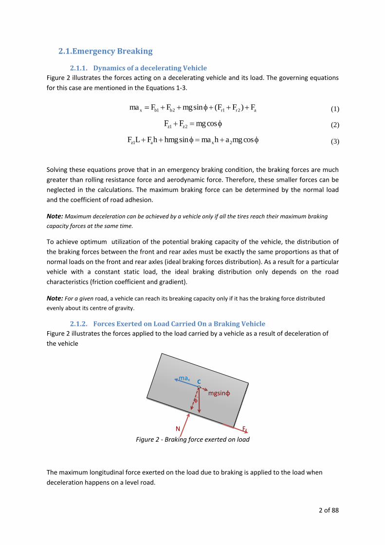
2.1.2. Forces Exerted on Load Carried On a Braking Vehicle

Figure 2 illustrates the forces applied to the load carried by a vehicle as a result of deceleration of

the vehicle

Figure 2 - Braking force exerted on load

The maximum longitudinal force exerted on the load due to braking is applied to the load when

deceleration happens on a level road.

max

mgsinφ

Ff N

C

φ

3 of 88

Longitudinal slip

Bra

kin

g fo

rce

Sliding

value μsW

Peak value μpW

Equation 4 shows the relationship for the calculating the maximum acceleration applied to the load.

As it can be seen the acceleration is only and directly dependant to the weight of the load and truck

and the friction coefficient between the tire and surface of the road.

mgF xmaxb (4)

2.1.2.1. Friction Coefficient

Friction coefficient is a function of the tire longitudinal slip, as shown in Figure 3 (Wong, 2001)

Figure 3 - Braking force – slip curve

It is also dependent on vehicle velocity, vertical load, tire inflation pressure etc. The average peak

and sliding values of the coefficient of road adhesion are given in Tables 1 and 2.

Table 1 Average Values of Coefficient of Road Adhesion (Wong, 2001)

Surface Peak Value μp Sliding value μs

Asphalt and concrete (dry) 0.8 – 0.9 0.75

Asphalt (wet) 0.5 – 0.7 0.45 – 0.6

Concrete (wet) 0.8 0.7

Gravel 0.6 0.55

Earth road (dry) 0.68 0.65

Earth road (wet) 0.55 0.4-0.5

Snow (hard-packed) 0.2 0.15

Ice 0.1 0.07

4 of 88

Table 2 Values of Coefficient of Road Adhesion for Truck Tires on Concrete Pavement at 64

km/h (40 mph) (Wong, 2001)

Tyre type Tyre construction

Dry Wet

μp μs μp μs

Goodyear Super Hi Miler (rib) Bias-ply 0.850 0.596 0.673 0.458

General GTX (rib) Bias-ply 0.826 0.517 0.745 0.530

Firestone Transteel (rib) Radial-ply 0.809 0.536 0.655 0.477

Firestone Transport 1 (rib) Bias-ply 0.804 0.557 0.825 0.579

Goodyear Unisteel R-1 (rib) Radial-ply 0.802 0.506 0.700 0.445

Firestone Transteel Traction (lug) Radial-ply 0.800 0.545 0.600 0.476

Goodyear Unisteel L-1 (lug) Radial-ply 0.768 0.555 0.566 0.427

Michelin XZA (rib) Radial-ply 0.768 0.524 0.573 0.443

Firestone Transport 200 (lug) Bias-ply 0.748 0.538 0.625 0.476

Uniroyal Fleet Master Super Lug Bias-ply 0.739 0.553 0.513 0.376

Goodyear Custom Cross Rib Bias-ply 0.716 0.546 0.600 0.455

Michelin XZZ (rib) Radial-ply 0.715 0.508 0.614 0.459

Average 0.756 0.540 0.641 0.467

In a recent PhD study supervised by Professor Reza Jazar (RMIT University), the experimental data

show that the maximum friction coefficient that can be reached by light vehicles is 0.96. The

experiment was conducted in Australia, Victoria, for the Victorian police force. (Hartman, 2014)

The maximum value 0.96 is for various weather and road surface conditions and light vehicles with

enhanced braking performance.

In the case of heavy trucks the highest value for friction coefficient found in the literature is slightly

lower than 0.8. This can be justified by considering the materials used for different types of tires.

The softer the rubber material used for making a tire is the higher friction coefficient between its

surface and the surface of the road and lower life expectancy will be. The softest types of tires are

used for Formula 1 cars which can be used only so a limited number of labs. The tires made for

heavy trucks usually have a minimum life expectancy of around 80000 kilometres which is at least

two times of the life of the tires for passenger vehicles such as Holden Commodore used for the

above mentioned experiments.

In British and New Zealand standards the value for friction coefficient equal to 1 has been used. The

investigating team believes that 0.8 is sufficient for providing safe carriage of loads but for the

purpose of a sensitivity analysis the requirements for the restraining equipment to maintain the

loads safely have been calculate for both 0.8g and 1g forward acceleration. These results are

available in the appendix B for 0.8g and appendix C for 1g.

It has been proven that the maximum acceleration applied to the load in a decelerating

scenario is directly dependant to the friction coefficient between the tire and the surface of

the road which will result in the following relation:

Maximum Forward acceleration applied to the load on a decelerating heavy vehicle:

0.8g

5 of 88

2.2. Hard Acceleration Assuming that there is adequate power from the engine, acceleration may be limited by the friction

between tire and road. The dynamics of an accelerating vehicle is presented here is similar to that of

braking.

Figure 4 - Dynamics model of an accelerating vehicle

Figure 4 and Equations 5-7 show the forces acting on an accelerating vehicle and its governing

equations.

a2r1rx2t1t F)FF(sinmgmaFF (5)

cosmgFF 2z1z (6)

cosmgasinhmghmahFLF 2xaa1z (7)

Note: Maximum acceleration of a vehicle can happen only when all the tires reach their maximum traction at

the same time.

Theoretically, the traction-limited acceleration is similar to that of the braking. However, the

practical maximum forward acceleration, especially for heavy vehicles, mainly depends on engine

power and transmission system. Otherwise the equation looks very similar and depends on the same

factors as before. The difference is that for braking every vehicle has to reach a minimum stopping

force in order to stop but for accelerating the engine plays an important role. In other words in

almost every vehicle (excluding the super-fast cars which are powered by stronger than required

engines and are lighter than normal cars) reaching to a level that the maximum static friction

coefficient is exceeded is highly dependent to the engine power.

2.2.1. Power-limited Acceleration

The ratio of engine power to vehicle weight is the first-order determinant of maximum acceleration.

At low speeds, the maximum acceleration can be obtained by neglecting all resistance forces acting

on the vehicle.

mg

ha

Fz1

Ft2

Ft1

Fr1

Fr1

max

Fa

h

a1

L a2

Fz2

6 of 88

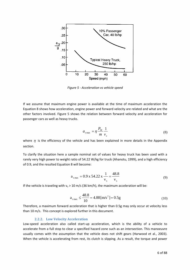
Figure 5 - Acceleration vs vehicle speed

If we assume that maximum engine power is available at the time of maximum acceleration the

Equation 8 shows how acceleration, engine power and forward velocity are related and what are the

other factors involved. Figure 5 shows the relation between forward velocity and acceleration for

passenger cars as well as heavy trucks.

x

Mx

vm

Pa

1max (8)

where is the efficiency of the vehicle and has been explained in more details in the Appendix

section.

To clarify the situation here a sample nominal set of values for heavy truck has been used with a

rarely very high power to weight ratio of 54.22 W/kg for truck (Ahanotu, 1999), and a high efficiency

of 0.9, and the resulted Equation 8 will become:

xx

maxxv

8.48

v

1 x 22.54 x 9.0a (9)

If the vehicle is traveling with vx > 10 m/s (36 km/h), the maximum acceleration will be:

0.5g ][m/s 88.410

8.48a 2

maxx (10)

Therefore, a maximum forward acceleration that is higher than 0.5g may only occur at velocity less

than 10 m/s. This concept is explored further in this document.

2.2.2. Low Velocity Acceleration

Low-speed acceleration also called start-up acceleration, which is the ability of a vehicle to

accelerate from a full stop to clear a specified hazard zone such as an intersection. This manoeuvre

usually comes with the assumption that the vehicle does not shift gears (Harwood et al., 2003).

When the vehicle is accelerating from rest, its clutch is slipping. As a result, the torque and power

7 of 88

are less than normal driving conditions. Therefore, Equation (8) and items mentioned in the

appendix about efficiency are not applicable to determine the low-speed acceleration.

Low-speed accelerating is usually modelled based on the observational data. Many researches have shown that linearly-decreasing acceleration rates well represent both maximum vehicle acceleration capabilities as well as actual motorist behaviour (Long, 2000). Utilizing the model, the acceleration of the vehicle is a function of vehicle speed v and the grade G:

Ggva x (11)

where, ax is the forward acceleration, α presents the maximum acceleration, which occurs at zero

speed, as it starts and β represents the slope of the line or the rate of decrease in acceleration as

speed, v, increases.

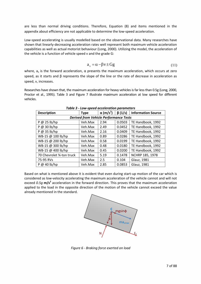
Researches have shown that, the maximum acceleration for heavy vehicles is far less than 0.5g (Long, 2000, Proctor et al., 1995). Table 3 and Figure 7 illustrate maximum acceleration at low speed for different vehicles.

Table 3 - Low-speed acceleration parameters

Description Type α (m/s2) β (1/s) Information Source

Derived from Vehicle Performance Tests

P @ 25 lb/hp Veh.Max 2.94 0.0503 TE Handbook, 1992



WB-15 @ 100 lb/hp Veh.Max 0.89 0.0286 TE Handbook, 1992




70 Chevrolet ¾-ton truck Veh.Max 5.19 0.1478 NCHRP 185, 1978

75-95 RVs Veh.Max 2.5 0.104 Glauz, 1981

P @ 40 lb/hp Veh.Max 2.85 0.0853 Glauz, 1981

Based on what is mentioned above it is evident that even during start-up motion of the car which is considered as low-velocity accelerating the maximum acceleration of the vehicle cannot and will not exceed 0.5g m/s2 acceleration in the forward direction. This proves that the maximum acceleration applied to the load in the opposite direction of the motion of the vehicle cannot exceed the value already mentioned in the standard.

Figure 6 - Braking force exerted on load

maxmax

mgsinφ

Ff N

C

φ

8 of 88

Figure 7 - Acceleration vs. vehicle speed

Figure 6 illustrates the forces applied to the load during a forward acceleration manoeuvre.

2.2.3. Maximum rearward braking deceleration

The ratio between the front braking force and the rear one is usually designed in a way that the

braking vehicle (in forward direction) can utilise much of the available tyre-road friction such as

illustrated in Figure 3.1. When the vehicle is braking, the normal force at front wheels increases

while that of rear wheels decreases. Therefore, the brake system is usually designed to provide more

braking force to the front wheels rather than at the rear.

When the vehicle is travelling rearwards and braking, the braking forces generated at the front and

rear wheels are reverse to what is expected in forward braking. This means that, the front wheels

will lock well before the rear wheel reaches it braking force capacity leading to a lower maximum

deceleration.

The following graph show the maximum braking capacity (in proportion of “g”) in rearward

direction. The graphs are produced by running the simulation with a braking force distribution

inverse of what used for the forward braking: : crwd = 1/cfwd= 1/c

9 of 88

Figure 8 – Maximum rearward deceleration vs. friction coefficient

The blue-dash line disappears as the μ0 value is calculated to be negative (-0.714) which means that

the front wheels always lock when rearward braking have not reached its capacity, for any tyre-road

friction coefficient (from 0 to 1).

As can be seen from the graph, the maximum rearward deceleration on the road of μ = 0.8 is about

0.48g which is far less than that of forward direction. Running the simulation with different truck

specifications convince that the maximum rearward deceleration is 0.5g.

It has been proven that the maximum acceleration applied to the load in an accelerating and

reverse braking scenarios is directly dependant to the friction coefficient between the tire and

the surface of the road as well as the engine power and vehicle efficiency which will result in the

following relation:

Maximum Rearwards acceleration applied to the load on an accelerating heavy vehicle:

0.5g

10 of 88

2.3. Cornering

2.3.1. Dynamics of a Turning Vehicle

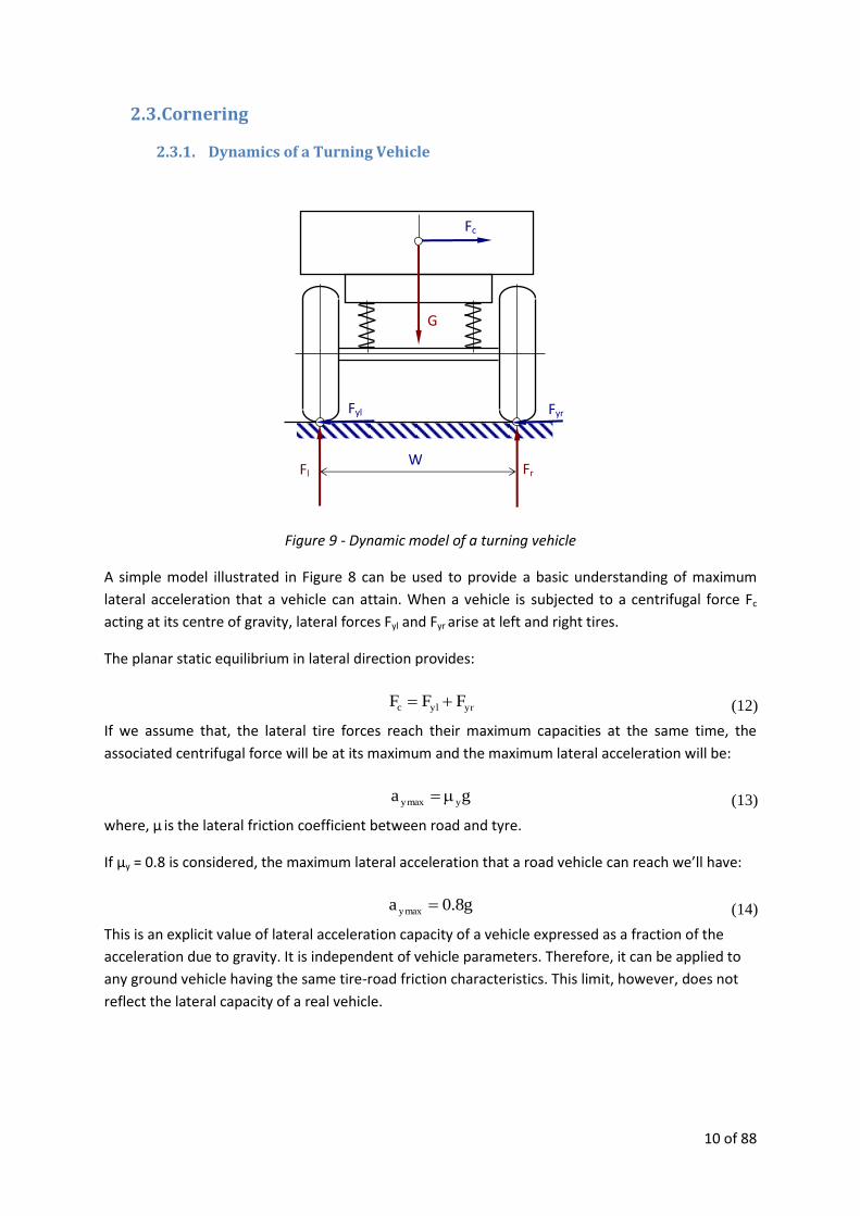
Figure 9 - Dynamic model of a turning vehicle

A simple model illustrated in Figure 8 can be used to provide a basic understanding of maximum

lateral acceleration that a vehicle can attain. When a vehicle is subjected to a centrifugal force Fc

acting at its centre of gravity, lateral forces Fyl and Fyr arise at left and right tires.

The planar static equilibrium in lateral direction provides:

yrylc FFF (12)

If we assume that, the lateral tire forces reach their maximum capacities at the same time, the

associated centrifugal force will be at its maximum and the maximum lateral acceleration will be:

ga ymaxy (13)

where, μ is the lateral friction coefficient between road and tyre.

If μy = 0.8 is considered, the maximum lateral acceleration that a road vehicle can reach we’ll have:

g8.0a maxy (14)

This is an explicit value of lateral acceleration capacity of a vehicle expressed as a fraction of the

acceleration due to gravity. It is independent of vehicle parameters. Therefore, it can be applied to

any ground vehicle having the same tire-road friction characteristics. This limit, however, does not

reflect the lateral capacity of a real vehicle.

G

Fc

Fyr Fyl

W Fr Fl

11 of 88

2.3.2. Practical Maximum Lateral Acceleration

In reality, the maximum lateral acceleration is much smaller than the value determined by Equation

(14) owing to the non-linear characteristics of the rubber tires, load transfer and other effects.

The lateral force of a tire is a function of side slip angle, normal load, etc. As illustrated in Figure 9,

the lateral force changes with the side slip angle, which reaches a maximum value at a certain angle,

beyond which the force levels off or reduces while much of the adhesion friction in the contact patch

is not utilized.

Figure 10 - Lateral force as a function of side slip angle

The lateral force also increases with the normal load under the tire in terms of a saturating curve, as

shown in Figure 10. Therefore, when the vehicle is cornering, the total lateral forces reduces as there

is a normal load transfer between the left and the right wheels, as depicted in Figure 11. These

effects, limit the cornering capacity of the vehicle as the outer tire has not been exploited to its

lateral capacity when the lateral force of the inner wheel is saturated and starts to skid off, which is

a major concern in vehicle handling safety.

Figure 11 – Load Saturation curve

12 of 88

Figure 12 - Lateral force reduction

Taking these effects into account, the real maximum lateral acceleration of a vehicle, therefore, less

than that determined in Equation (14).

2.3.3. Planar Non-Linear Model

The relationship between the lateral capacity and vehicle parameters is implicit. Hence, to

determine the lateral acceleration limit for a particular vehicle, programming on a computer is most

often the preferred method.

A planar model of a rear-wheel-drive single unit vehicle, illustrated in Figure 13, is usually utilized to

investigate the lateral dynamics.

Figure 13 - Dynamic model of a turning vehicle

The Newton-Euler equations of motion for a rigid vehicle in the body coordinate frame B, which is

the frame attached to the vehicle at its centre of gravity C, are:

0 2 4 6 8 10 12 14 16 18 200

1000

2000

3000

4000

5000

6000

sideslip angle (deg)

Fy (

N)

Fz=2(KN)

Load shift: inner tire

Fz=6(KN)

Load shift: outer tire

Fz=4(KN)

No load shift

Increase

Decrease

0 1 2 3 4 5 6 70

500

1000

1500

2000

2500

Fz (KN)

Fy (

N)

FzoFzi

reduction

Fy1 Fy2

Fy3 Fy4

Fx4 Fx3

Mz1 Mz2

Mz3 Mz4

y

x

C

B

w

13 of 88

yxx mrvvmF (15)

xyy mrvvmF (16)

zz IrM (17)

where, vx, vy, are longitudinal, lateral velocity of the vehicle centre expressed in the body coordinate

frame, r is the yaw rate of the vehicle, m presents the weight of the vehicle, Iz is the rotational inertia

of the vehicle about Cz

A force system will be acting on the vehicle which is explained in more details in the appendix

section. The equation of motion resulted from this force system have been solved using a Simulink

model (schematic view available in the appendix section) and the following are the results.

Figures 14-17 shows normal forces, lateral forces, saturated lateral forces under the tires of a typical

truck, and the lateral acceleration of the vehicle during the manoeuvre.

Figure 14 - Normal forces under the vehicle tires

Figure 15 - Lateral forces under the vehicle tires

14 of 88

Figure 16 - Lateral forces, and their saturated values under the tires

Figure 17 - Lateral acceleration of the vehicle

15 of 88

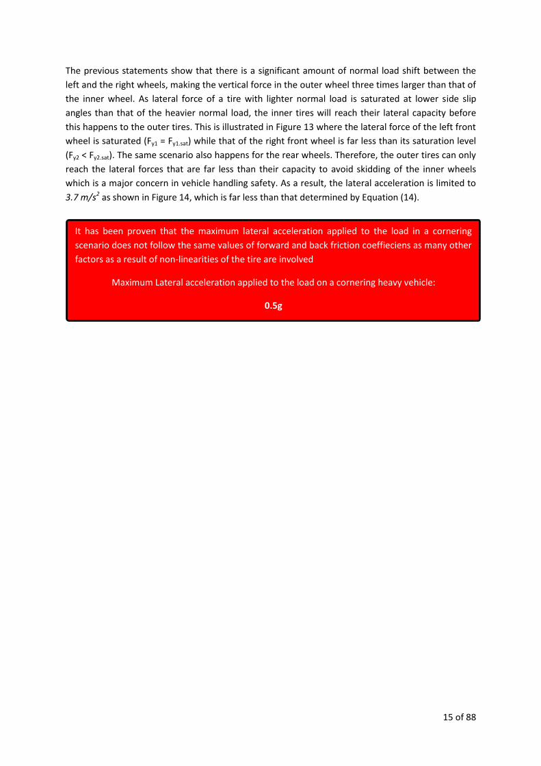
The previous statements show that there is a significant amount of normal load shift between the

left and the right wheels, making the vertical force in the outer wheel three times larger than that of

the inner wheel. As lateral force of a tire with lighter normal load is saturated at lower side slip

angles than that of the heavier normal load, the inner tires will reach their lateral capacity before

this happens to the outer tires. This is illustrated in Figure 13 where the lateral force of the left front

wheel is saturated (Fy1 = Fy1.sat) while that of the right front wheel is far less than its saturation level

(Fy2 < Fy2.sat). The same scenario also happens for the rear wheels. Therefore, the outer tires can only

reach the lateral forces that are far less than their capacity to avoid skidding of the inner wheels

which is a major concern in vehicle handling safety. As a result, the lateral acceleration is limited to

3.7 m/s2 as shown in Figure 14, which is far less than that determined by Equation (14).

It has been proven that the maximum lateral acceleration applied to the load in a cornering

scenario does not follow the same values of forward and back friction coeffieciens as many other

factors as a result of non-linearities of the tire are involved

Maximum Lateral acceleration applied to the load on a cornering heavy vehicle:

0.5g

16 of 88

2.4. Jack-knifing Jack-knifing occurs for different reasons, for example if the rear wheels of the truck are blocked,

when the vehicle applies the brakes abruptly while cornering, or when the road has low adherence

(Bouteldja et al.). Therefore, the manoeuvre is modelled by different scenarios. By neglecting the

roll, pitch, and bounce motions, the model in Figure 18 can be used to describe the dynamics of jack-

knifing. The model includes a truck with two axles, and a semitrailer connected to the truck through

the fifth wheel.

Figure 18 - Dynamics of a tractor-semitrailer combination

Despite the fact that, the model has been simplified, the equations of motion(see Appendix for more

details) remain extremely lengthy and complex (Mikulcik, 1971). Moreover, the dynamic behaviour

of the articulated vehicle is affected by many different factors such as braking force, cornering force,

friction coefficient under each tire, etc. Considering the time restrictions, the complexity of the

dynamics and the variety of factors involved in the happening of jack-knifing, the general dynamics

of the truck-semitrailer combination has not been modelled.

During jack-knifing the dynamic friction coefficient cannot be used as a result of sliding of some of

the tires if not all. In order to consider some calculations using the static friction coefficients are

needed. This adds a lot of complications to the calculations which is why the dynamic behaviour of

the motion of trucks in the mentioned scenario has not been fully investigated by researchers

previously.

RMIT University believes that this will cause situations beyond the normal driving scenarios covered

by the performance standard and a full investigation that will take into account enough variables to

present a valid conclusion will require a much longer period.

17 of 88

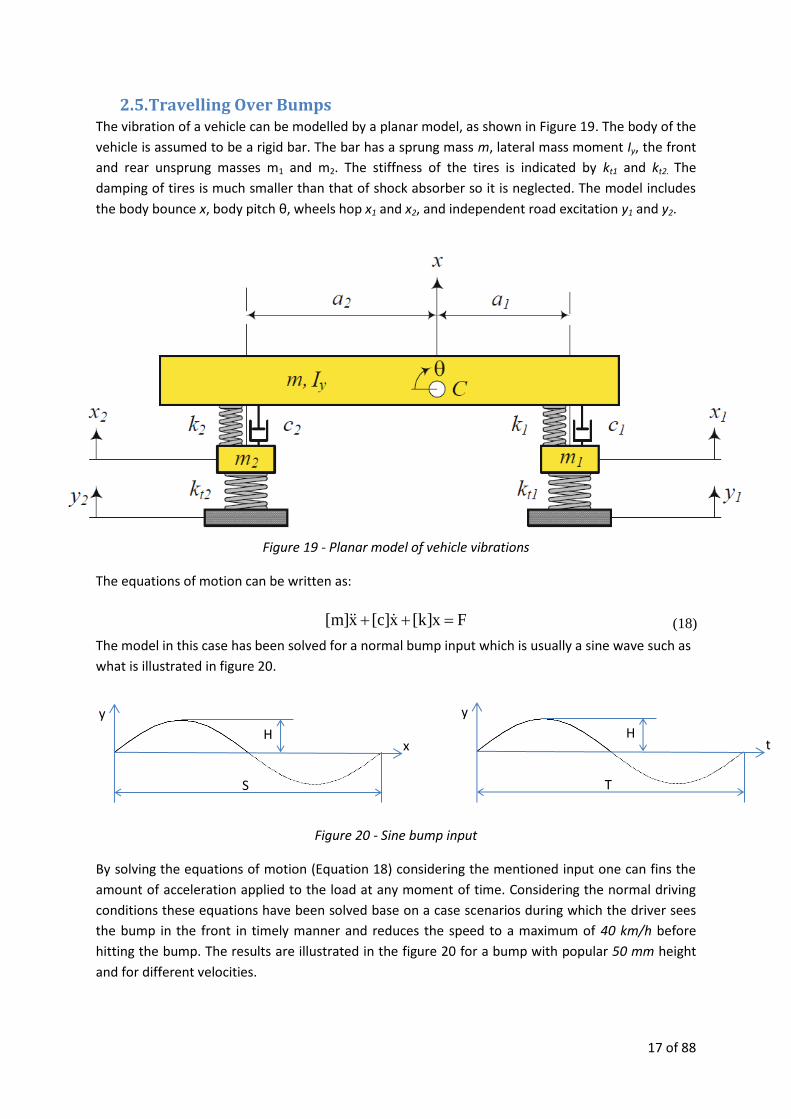
2.5. Travelling Over Bumps The vibration of a vehicle can be modelled by a planar model, as shown in Figure 19. The body of the

vehicle is assumed to be a rigid bar. The bar has a sprung mass m, lateral mass moment Iy, the front

and rear unsprung masses m1 and m2. The stiffness of the tires is indicated by kt1 and kt2. The

damping of tires is much smaller than that of shock absorber so it is neglected. The model includes

the body bounce x, body pitch θ, wheels hop x1 and x2, and independent road excitation y1 and y2.

Figure 19 - Planar model of vehicle vibrations

The equations of motion can be written as:

Fx]k[x]c[x]m[ (18)

The model in this case has been solved for a normal bump input which is usually a sine wave such as

what is illustrated in figure 20.

Figure 20 - Sine bump input

By solving the equations of motion (Equation 18) considering the mentioned input one can fins the

amount of acceleration applied to the load at any moment of time. Considering the normal driving

conditions these equations have been solved base on a case scenarios during which the driver sees

the bump in the front in timely manner and reduces the speed to a maximum of 40 km/h before

hitting the bump. The results are illustrated in the figure 20 for a bump with popular 50 mm height

and for different velocities.

H x

y

S

H t

y

T

18 of 88

It should be noted the maximum acceleration value is calculated based on a maximum height of the

bump to be 100mm. If the height of the bump is more than 100mm then it is evident that the

vertical acceleration will exceed the 0.2g threshold and is not considered as normal driving condition

as a result.

Figure 21 - Body vertical acceleration at different speeds

Same has been done for a constant velocity of 20 km/h but for different lengths of the bumps which

can be seen in Figure 22.

19 of 88

Figure 22 - Body vertical acceleration for different bump lengths

As it can be seen in none of the mentioned cases the acceleration goes over 0.2g m/s2.

In order to study the situation farther the equations were re-arranged and solved again this time to

find out the sensitivity of the system to the changes of velocities. In other words it can be seen in

figures 23-27 that the maximum vertical acceleration applied to the load only exceeds the above

mentioned threshold when the length of the bump is more than 2000 mm which is very unlikely to

happen no matter what the velocity of the vehicle is.

Figure 23 -maximum vertical acceleration for different vehicle velocity (S = 700 mm)

20 of 88

Figure 24 - Maximum vertical acceleration for different vehicle velocity (S = 1000 mm)


21 of 88


Figure 27 -Maximum vertical acceleration for different vehicle velocity (S = 3000 mm)

22 of 88

2.6. Minor Collision

2.6.1. Dynamics of Vehicle Collisions

The majority of vehicle collisions in reality involve frontal impact. It is also the most important type

of impact test. Therefore, in this section, the dynamics of frontal collisions is considered. The model

is shown in Figure 28.

Figure 28 - Dynamics model of vehicle collision

Consider vehicle A, and vehicle B with their masses M, and m, respectively. V, v are the velocities of

the vehicles at any time during the impact. Subscript 1 stands for all conditions at the moment of

first contact; and 2 is for conditions at the moment when contact is lost. During the impact, there is

a force P, and a linear impulse t

1t

PdtI act between the vehicles up to any time t.

The momentum equations are used. See more details in the appendix section.

If p denotes the summation of v and V (p = v + V), the new parameter will change in the manner

shown in Figure 29.

Figure 29 - p changes with time

In the first phase during the (t1 – t0) period of time, the compression and distortion occur and that is

when p decreases to zero and the two vehicle are moving together. In the second phase, a portion of

elastic strain energy in the vehicles structures is restored, and the vehicles finally separate with a

negative relative velocity p2.

The maximum vertical acceleration applied to the load on a vehicle which is traveling

over a bump can exceed the value below only if the length of the bump is over

2000mm or if the height is over 100mm which are not considered as a normal driving

condition.

Maximum Vertical acceleration applied to the load on a heavy vehicle travelling over

a bump in normal driving conditions:

0.2g

V v I I M m A

B

p

p1

p2

t1 t0 t2 t

23 of 88

Using the Newton’s law of restitution and using the Coefficient of restitution (e) the following can be

used:

12 epp (19)

The Newton’s law Equation (19), coupled with the momentum equations (available in the appendix)

are sufficient to determine the final velocities of the two vehicle after the collision. The whole

problem will end to be a system of three equations. Solving these simultaneously will yield the

following for the relative velocity of the two vehicles involved in the collision after during the second

phase:

)vV)(e1(

1m

M

1VVV 1121

(20)

2.6.2. Special Cases

In this section some scenarios have been studied which might include special situations. It has been

tried to highlight most of the happenings during a collision in this section.

1. Vehicle A with Mass M travelling at 30km/h collides with vehicle B with m traveling at the same

velocity

The relative velocity after the collision can be calculated using Equation (20). As the real impact

practically lasts for about 1/10 second (Macmillan, 1983), in this estimation we assume that Δt =

t2 – t1 = 0.1 (s). Therefore, the average deceleration that the vehicle B experiences is:

)1(

1

7.166. e

M

mt

va crashx

(21)

The average deceleration rate of the vehicle B is illustrated in Figure 26 with the minimum value

of 15.15 m/s2 associated with e = 0 (totally inelastic) and m/M = 10;

24 of 88

Figure 30 - Average deceleration of the vehicle for wide ranges of e and m/M

As it can be seen from the figure Deceleration starts at a very large value and gets bigger as the

weights of the two Vehicles get closer to each other.

2. Vehicle B with mass m travelling at 30 Km/h and collides with a fixed block

Again using the same steps as before the relative velocity is found using Equation (20). It should

be noted that in this case the weight of a second vehicle which is considered to a block would be

infinity and its velocity zero.

Therefore the average velocity is:

)(m/s 3.833.83)e1(t

va 2

crash.x

(22)

Figure 31 illustrates the average deceleration for different vehicle velocities.

25 of 88

Figure 31 - Average deceleration of the vehicle for different vehicle speeds

It can be clearly seen from the graph, that the average deceleration is very high during these

scenarios, even when the vehicle is travelling at 1 m/s speed (aave > g).

In reality, the deceleration is not constant. As a result, the maximum deceleration must be much

greater than what is defined above. Therefore, the collision scenario should not be considered to

be a normal driving condition when it comes to the load restraint system calculation. To study

the matter farther in the next session it has been tried to find out at what vehicle velocities the

acceleration applied to the load and vehicle will exceed the threshold value determined earlier

in this study for the forward direction.

2.7. Velocity by which the average acceleration of 0.8g is resulted (Critical Velocity)

In this section the problem has been solved again for both of the above cases but this time the focus

will be on the velocity by which the deceleration exceeds the 0.8g threshold determined earlier in

this study. We call this the Critical Velocity. The solutions and more details can be found in the

appendixes. Figure 32 illustrates the result for the critical velocity for a truck colliding with another

vehicle with different masses. The heavier the other vehicle the bigger is the deceleration value. It is

interesting to see that with velocities slightly more than 1m/s the 0.8g threshold is exceeded not

matter how heavy the other vehicle is.

26 of 88

Figure 32 - Velocity at which the 0.8g deceleration occurs for wide ranges of e and m/M

Graph 33 is illustrating the case during which a truck hits a fixed block. The critical velocity changes

with respect to the materials of the vehicle and the block which determine the coefficient of

restitution. But the situation is not any better and the same is resulted here too. All the above

mentioned proves that the front collisions cannot be considered as a normal driving condition. The

deceleration is so high during this case that restraining the load can hardly be achieved by the values

mentioned and used for the present standards.

Figure 33 - Velocity at which the 0.8g deceleration occurs for different e

27 of 88

3. Forces Required to Restrain Loads

3.1. Tie-Down Lashing The main reason to vertically restraint a load on a vehicle, shown in Figure 34, is to produce friction

force Ff countering the inertial force k.W which acts at the centre of gravity of the load. The friction

force results from W and restraint system clamping force Fc; where, W presents weight of the cargo,

k is the coefficient of acceleration (0.8 forward, 0.5 rearward, and 0.5 sideward), Fc is the

clamping force produced by the restraint equipment

Figure 34 - Restraint force

Equations and lashing requirements are available in the appendixes. The lashing requirement has

been recalculated and illustrated again based on the findings of this study, in more details.

3.1.1. Symmetric Tensioning Forces

Figure 35 - Tensioning force needed to safely restraint load

The tension force required and the maximum weight each lashing can carry is calculated for both

sliding balance and tipping balance cases.

NOTE: In cases that the friction coefficient between load and the loaded surface of the truck is bigger than

acceleration coefficient the lashing must be pre-tensioned to provide a minimum clamping force equal to 20%

of the weight of the load.

W

k.W

Fc

Ff

h

b

h

b

k.W

W

28 of 88

This is because the load must always remain in contact with the deck even if road vibration and over

travelling bumps forces are applied in order to maintain the friction force during normal driving

conditions.

3.1.2. Asymmetric Tensioning Forces

Unexpected forces that are applied to the load during travelling are inevitable. These scenarios can

be studied by taking an asymmetric lashing arrangement in to consideration.

Figure 36 illustrates a situation in which the lashing can be deflected by changing the angle α. The

tensioning force is reduced by the value c = e-μ’α, where μ’ is the friction coefficient between the

cargo and the lashing belt according to Eytelwein's formula. Moreover, the asymmetry also creates

horizontal force, as shown in Figure 37.

Figure 36 - Asymmetric restraint forces

Figure 37 - Clamping force needed to safely restraint load

h

b

k.

W

W

29 of 88

The tensioning force needed, during the worst case scenarios, to safely restraint load on the vehicle

are calculated for sliding and tipping balance cases and are available in the appendixes.

NOTE: In every mentioned case above the maximum lashing force required is highly and directly dependant to

the direction of motion and the friction coefficient of the loaded surface of the truck. As a result the use of

coarse material for the bottom section of the truck which in contact with the bottom of the load is

recommended.

3.2. Suggested Safety Factor for Lashing Equipment In another attempt for more safely carrying of the load it is important that a safety factor is used and

multiplied to the required lashing force before the number of lashings is determined and the tables

for this value are used from the standard.

The suggested safety factor against the lashing angle is illustrated by Figures 38 and 39 for different

friction coefficient values.

Figure 38 - Lashing safety factor for μ = 0.8, and different μ’

30 of 88

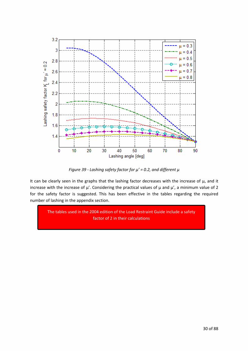
Figure 39 - Lashing safety factor for μ’ = 0.2, and different μ

It can be clearly seen in the graphs that the lashing factor decreases with the increase of μ, and it

increase with the increase of μ’. Considering the practical values of μ and μ’, a minimum value of 2

for the safety factor is suggested. This has been effective in the tables regarding the required

number of lashing in the appendix section.

The tables used in the 2004 edition of the Load Restraint Guide include a safety

factor of 2 in their calculations

31 of 88

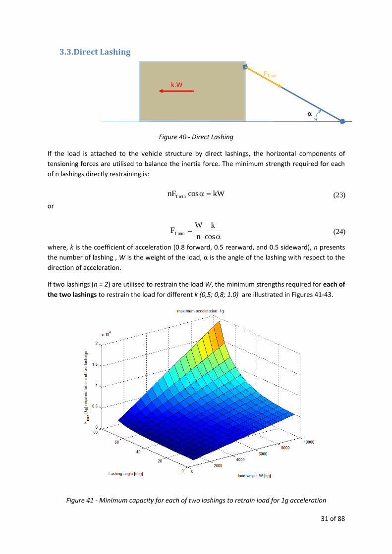
3.3. Direct Lashing

Figure 40 - Direct Lashing

If the load is attached to the vehicle structure by direct lashings, the horizontal components of

tensioning forces are utilised to balance the inertia force. The minimum strength required for each

of n lashings directly restraining is:

kWcosnF minT (23)

or

cos

k

n

WF minT (24)

where, k is the coefficient of acceleration (0.8 forward, 0.5 rearward, and 0.5 sideward), n presents

the number of lashing , W is the weight of the load, α is the angle of the lashing with respect to the

direction of acceleration.

If two lashings (n = 2) are utilised to restrain the load W, the minimum strengths required for each of

the two lashings to restrain the load for different k (0,5; 0,8; 1.0) are illustrated in Figures 41-43.

Figure 41 - Minimum capacity for each of two lashings to retrain load for 1g acceleration

α

k.W

FTmin

32 of 88

Figure 42 - Minimum capacity for each of two lashings to retrain load for 0.8g acceleration

Figure 43 - Minimum capacity for each of two lashings to retrain load for 0.5g acceleration

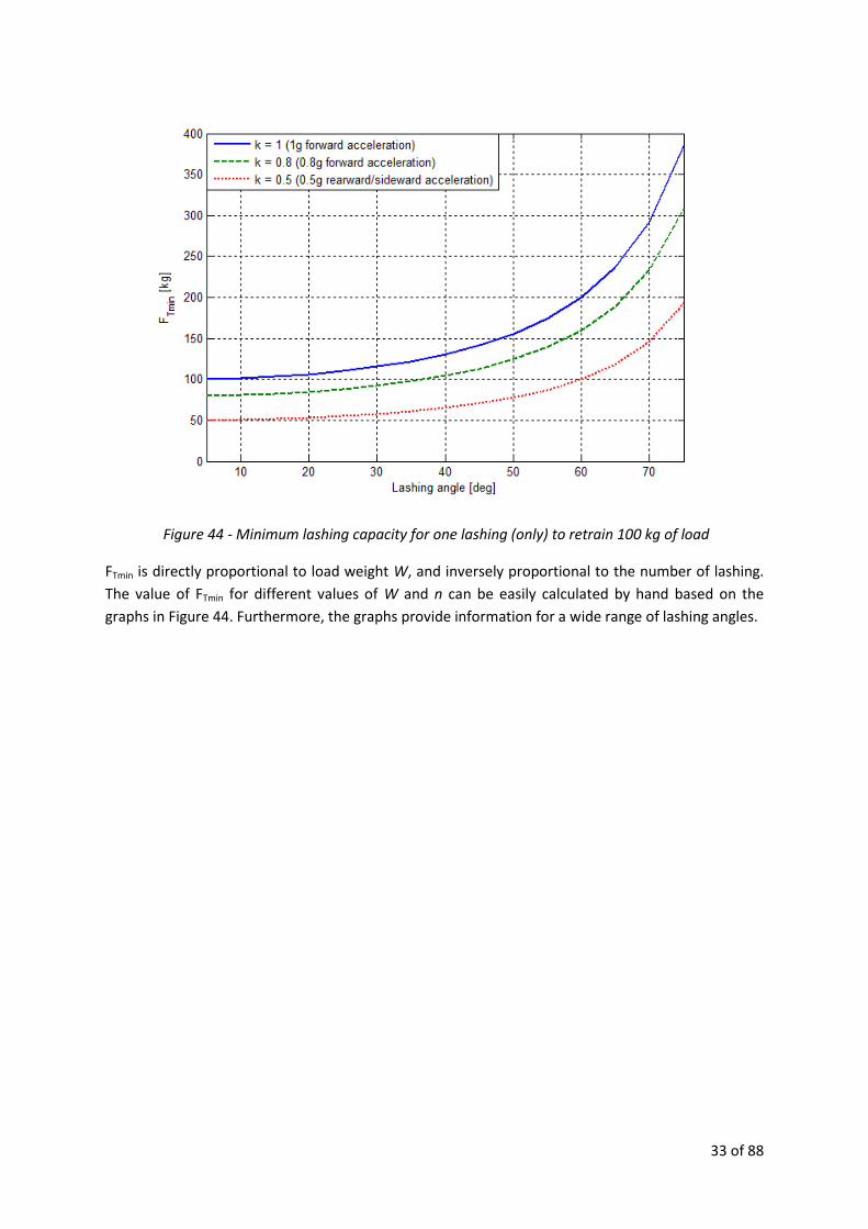
Figures 44 shows the minimum strength (lashing capacity) required for only one lashing to restrain

100 kg load with k = 0.8, and k = 0.5.

33 of 88

Figure 44 - Minimum lashing capacity for one lashing (only) to retrain 100 kg of load

FTmin is directly proportional to load weight W, and inversely proportional to the number of lashing.

The value of FTmin for different values of W and n can be easily calculated by hand based on the

graphs in Figure 44. Furthermore, the graphs provide information for a wide range of lashing angles.

34 of 88

4. Conditions Likely to Effect Better or Worse of the Safe Carriage of

Loads

4.1. Vehicle Parameters

4.1.1. Braking

In vehicles equipped with EBD/ABS systems, the maximum braking acceleration (deceleration) is μxg,

for a level road, as proved in Section 1. In this case, the available friction between tyres and road is

fully utilised. In vehicles without EBD, where the ratio of front braking force to rear braking force is

constant, the vehicles usually skid off when the available tyre-road friction is not utilised. Therefore,

the decelerations of these vehicles are usually less than those having EBD system.

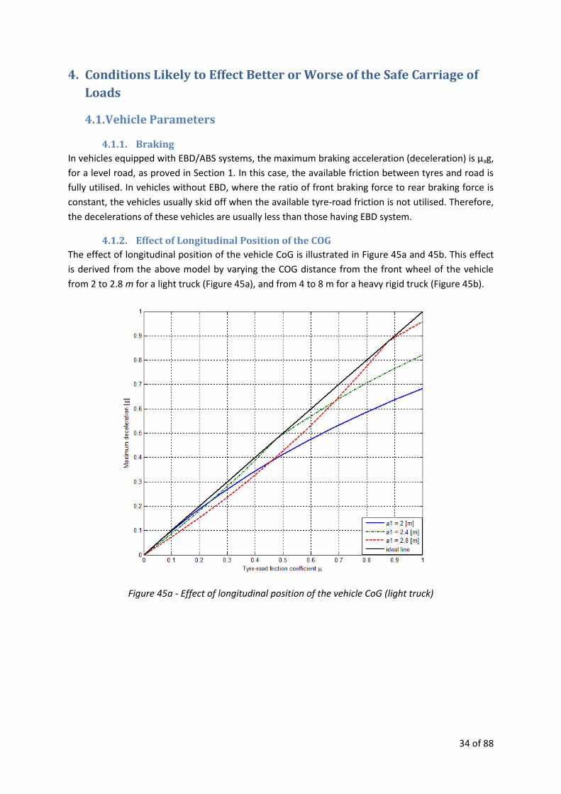
4.1.2. Effect of Longitudinal Position of the COG

The effect of longitudinal position of the vehicle CoG is illustrated in Figure 45a and 45b. This effect

is derived from the above model by varying the COG distance from the front wheel of the vehicle

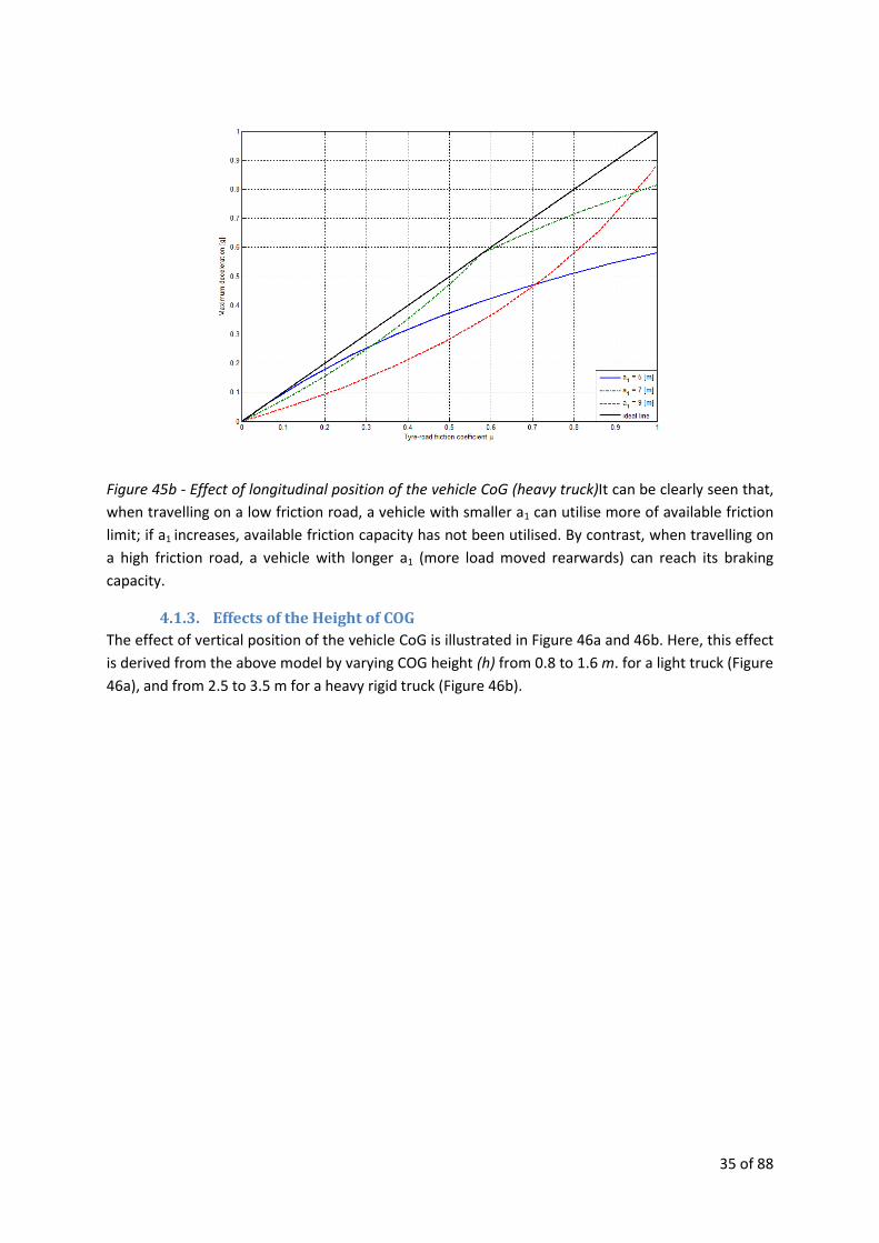
from 2 to 2.8 m for a light truck (Figure 45a), and from 4 to 8 m for a heavy rigid truck (Figure 45b).

Figure 45a - Effect of longitudinal position of the vehicle CoG (light truck)

35 of 88

Figure 45b - Effect of longitudinal position of the vehicle CoG (heavy truck)It can be clearly seen that,

when travelling on a low friction road, a vehicle with smaller a1 can utilise more of available friction

limit; if a1 increases, available friction capacity has not been utilised. By contrast, when travelling on

a high friction road, a vehicle with longer a1 (more load moved rearwards) can reach its braking

capacity.

4.1.3. Effects of the Height of COG

The effect of vertical position of the vehicle CoG is illustrated in Figure 46a and 46b. Here, this effect

is derived from the above model by varying COG height (h) from 0.8 to 1.6 m. for a light truck (Figure

46a), and from 2.5 to 3.5 m for a heavy rigid truck (Figure 46b).

36 of 88

Figure 46a - Effect of vertical position of the vehicle CoG (light truck)

Figure 46b - Effect of vertical position of the vehicle CoG (heavy truck truck)

37 of 88

As it is shown, when travelling on a low friction road, a vehicle with higher CoG can utilise more of

available friction limit. However, when the friction is high, a vehicle with lower CoG can reach its

braking capacity.

4.1.4. Effect of Braking Distribution

The effect of braking force distribution is illustrated in Figure 47. Here, this effect is derived from the

above model by varying c from 1.2 to 2.

Figure 47 - Effect of braking force distribution

Figure 47 shows that, when travelling on a low friction road, vehicle with a lower c (lower Fb1/Fb2)

can utilise more of the available friction limit. When the friction is high, a vehicle with higher c can

reach its braking capacity easier.

4.2. Cornering As mentioned in Section 1, the non-linear characteristics of the tyre and the load shift limit the

lateral force and hence lateral acceleration of the vehicle. The load shift is heavily influenced by the

vehicle CoG. If the load transfer between the inner and the outer wheels is large, the inner wheels

will be saturated at low side-slip angle (and lateral acceleration). Figures 48 and 49 show how the

vertical and longitudinal positions of the CoG affect the lateral capacity of the vehicle. The graphs

are extracted from the model built in the Section I by varying the height of CoG (h) and the distance

between the front axle and the CoG (a1), respectively.

38 of 88

Figure 48 - Effect of vertical position of the vehicle CoG on lateral acceleration

Figure 49 - Effect of longitudinal position of the vehicle CoG on lateral acceleration

39 of 88

It can be seen in Figure 48, the maximum lateral acceleration increases with the decrease of the

height of the CoG. This is because load transfer is proportional to the CoG height. The longitudinal

position of the CoG, however, has little effect on the sideward acceleration. This is due to the fact

that if the centre of gravity moves rearwards, the lateral force at font inner wheel is saturated first; if

it moves forwards, the lateral force at rear inner wheel is saturated first.

4.3. Vertical Vibration The effect of longitudinal position of the CoG on vertical acceleration is depicted in Figure 50, where

the a1 (distance between front axle and the CoG) is varied from 1.3m to 1.9m.

40 of 88

Figure 50 - Effect of longitudinal position of the vehicle CoG on vertical acceleration

As illustrated by the graphs, the CoG position applies some changes to the vertical acceleration but it

is not very important in this context as it is not exceeding the pre-determined acceleration values.

41 of 88

5. Suitable Performance Expectations for Load Restraint Equipment

All the restraint equipment must comply with relevant Australian standards. Therefore, the suitable

performance expectations for each should be the capacity, and requirements nominated in the

standard.

5.1. Chain Assemblies Performance

The performance expectations for chain assemblies must comply with AS/NZS 4344 (Motor vehicles-

Cargo restraint systems-Transport chain and components).

The minimum breaking strength and lashing capacity of the different chains are illustrated in Table 4.

Table 4 - Lashing capacity of chain

Nominal chain size

mm

Lashing capacity (LC)

kg

6 2300

7 2900

7.3 3000

8 3800

10 6000

13 9000

5.2. Webbing Load Restraint Systems

The performance expectations for chain must comply with AS/NZS 4380 (Motor vehicles-Cargo

restraint systems- Transport webbing and components).

The lashing capacities of the webbing restraint load system are illustrated in Table 5.

Table 5 - Lashing capacity of webbing trap and components

Description Lashing capacity (LC)

kg

25mm x 4m Ratchet Webbing Tie Down with hook each end 400

35mm x 6m Ratchet Webbing Tie Down with hook and keeper each end 1500

50mm x 9m Ratchet Webbing Tie Down with hook and each end 2500

75mm x 9m Ratchet Webbing Tie Down with hook and each end 5000

Clip on truck winch with reinforced legs

(complete with 50mm x 9m webbing strap with hook and keeper) 2500

Long handled pull down ratchet assembly to suit 50mm webbing 2500

42 of 88

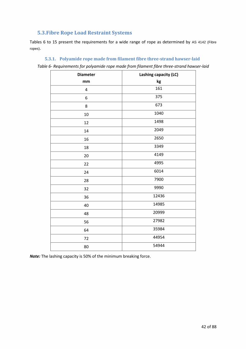
5.3. Fibre Rope Load Restraint Systems

Tables 6 to 15 present the requirements for a wide range of rope as determined by AS 4142 (Fibre

ropes).

5.3.1. Polyamide rope made from filament fibre three-strand hawser-laid

Table 6- Requirements for polyamide rope made from filament fibre three-strand hawser-laid

Diameter

mm


kg

4 161

6 375

8 673

10 1040

12 1498

14 2049

16 2650

18 3349

20 4149

22 4995

24 6014

28 7900

32 9990

36 12436

40 14985

48 20999

56 27982

64 35984

72 44954

80 54944

Note: The lashing capacity is 50% of the minimum breaking force.

43 of 88

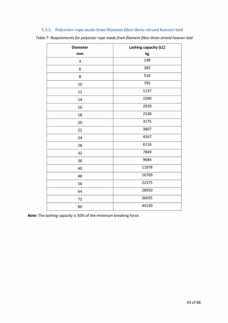
5.3.2. Polyester rope made from filament fibre three-strand hawser-laid

Table 7- Requirements for polyester rope made from filament fibre three-strand hawser-laid

Diameter

mm


kg

4 148

6 282

8 510

10 795

12 1137

14 1590

16 2029

18 2538

20 3175

22 3807

24 4567

28 6116

32 7849

36 9684

40 11978

48 16769

56 22375

64 28950

72 36035

80 44190


44 of 88

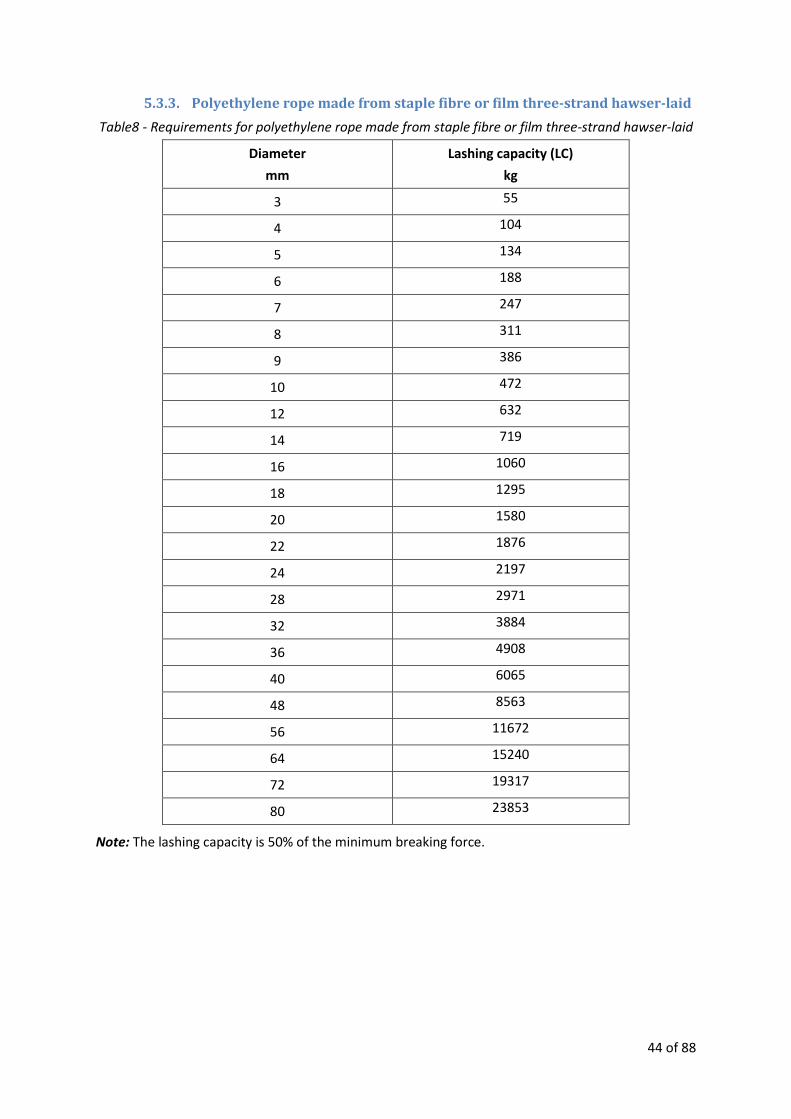
5.3.3. Polyethylene rope made from staple fibre or film three-strand hawser-laid

Table8 - Requirements for polyethylene rope made from staple fibre or film three-strand hawser-laid

Diameter

mm


kg

3 55

4 104

5 134

6 188

7 247

8 311

9 386

10 472

12 632

14 719

16 1060

18 1295

20 1580

22 1876

24 2197

28 2971

32 3884

36 4908

40 6065

48 8563

56 11672

64 15240

72 19317

80 23853


45 of 88

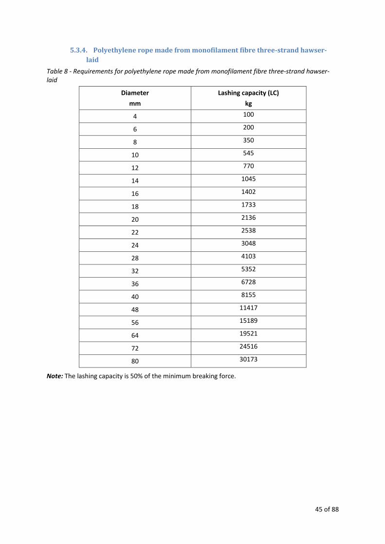
5.3.4. Polyethylene rope made from monofilament fibre three-strand hawser-

laid

Table 8 - Requirements for polyethylene rope made from monofilament fibre three-strand hawser-laid

Diameter

mm


kg

4 100

6 200

8 350

10 545

12 770

14 1045

16 1402

18 1733

20 2136

22 2538

24 3048

28 4103

32 5352

36 6728

40 8155

48 11417

56 15189

64 19521

72 24516

80 30173


46 of 88

5.3.5. Polyethylene rope made from film, monofilament, multifilament or staple

fibre three-strand hawser-laid

Table 9 - Requirements for polyethylene rope made from film, monofilament, multifilament or staple fibre three-strand hawser-laid

Diameter

mm


kg

4 107

6 228

8 530

10 780

12 1106

14 1524

16 1886

18 2406

20 2900

22 3476

24 4062

28 5352

32 6728

36 8461

40 10245

48 14271

56 18909

64 24465

72 30734

80 37768


47 of 88

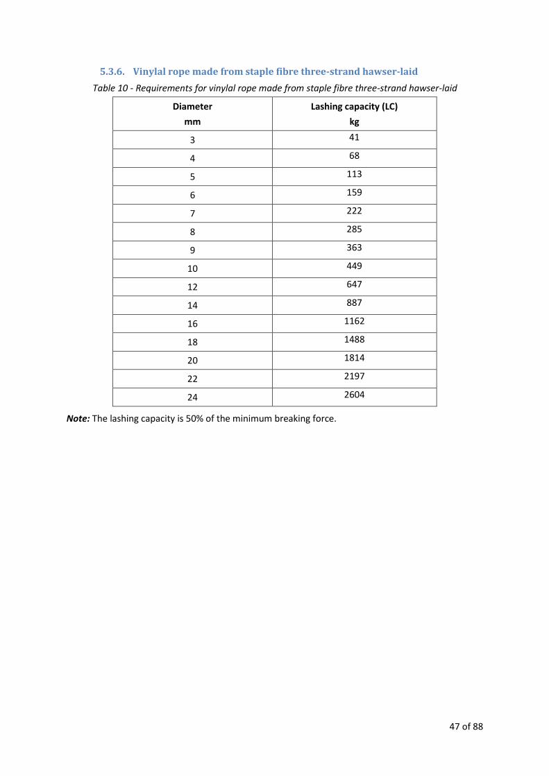
5.3.6. Vinylal rope made from staple fibre three-strand hawser-laid

Table 10 - Requirements for vinylal rope made from staple fibre three-strand hawser-laid

Diameter

mm


kg

3 41

4 68

5 113

6 159

7 222

8 285

9 363

10 449

12 647

14 887

16 1162

18 1488

20 1814

22 2197

24 2604


48 of 88

5.3.7. Polyamide rope eight-strand plaited

Table 11 - Requirements for polyamide rope eight-strand plaited

Diameter

mm


kg

16 2650

20 4149

24 6014

28 7900

32 9990

36 12436

40 14985

48 20999

56 27982

64 35984

72 44954

80 54944


49 of 88

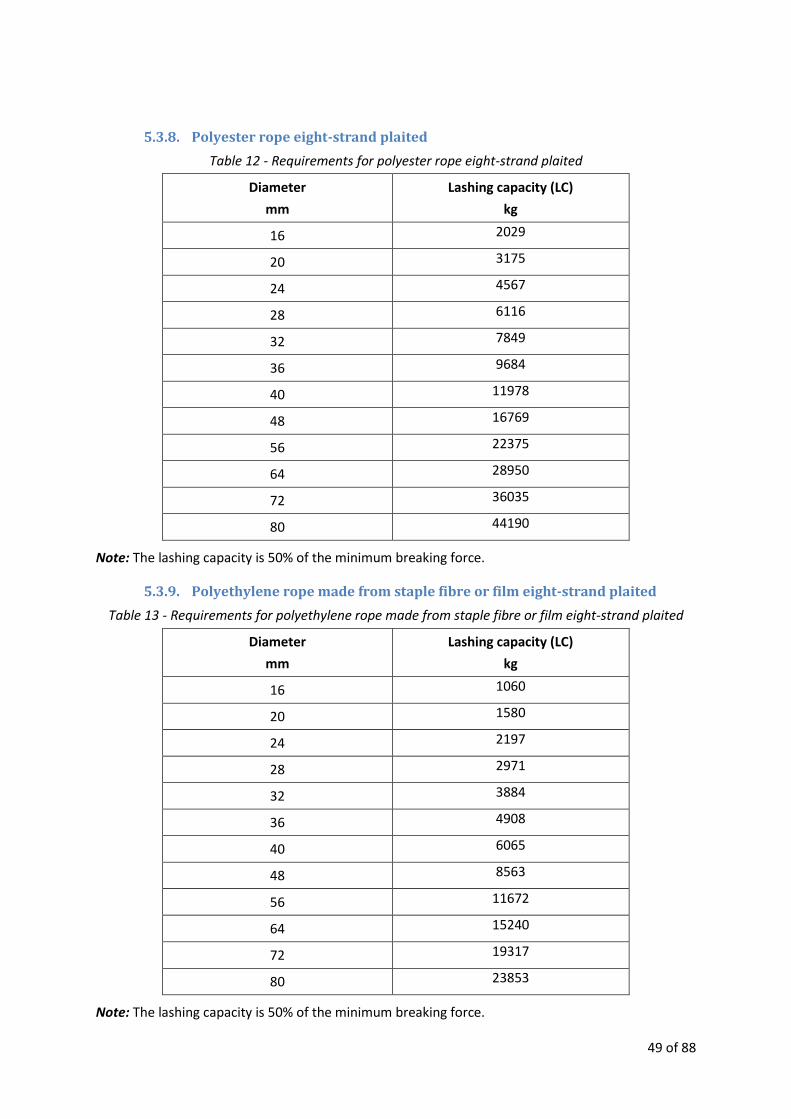
5.3.8. Polyester rope eight-strand plaited

Table 12 - Requirements for polyester rope eight-strand plaited

Diameter

mm


kg

16 2029

20 3175

24 4567

28 6116

32 7849

36 9684

40 11978

48 16769

56 22375

64 28950

72 36035

80 44190


5.3.9. Polyethylene rope made from staple fibre or film eight-strand plaited

Table 13 - Requirements for polyethylene rope made from staple fibre or film eight-strand plaited

Diameter

mm


kg

16 1060

20 1580

24 2197

28 2971

32 3884

36 4908

40 6065

48 8563

56 11672

64 15240

72 19317

80 23853


50 of 88

5.3.10. Polyethylene rope made from film, monofilament, multifilament or staple

fibre eight-strand plaited

Table 14 - Requirements for polyethylene rope made from film, monofilament, multifilament or staple fibre eight-strand plaited

Diameter

mm


kg

16 1886

20 2900

24 4062

28 5352

32 6728

36 8461

40 10245

48 14271

56 18909

64 24465

72 30734

80 37768


5.3.11. Steel wire rope load restraint systems

The following tables 4.14 and 4.15 present the minimum breaking force for a wide range of rope as

determined by AS 3569 (Steel Wire Ropes). For the wire ropes with different sizes and materials, refer

to AS 3569.

51 of 88

5.3.12. Steel wire rope grade 1570, galvanised

Table 15 - Minimum breaking force: grade 1570, galvanised

Diameter

mm


kg

Fibre core IWR or IWS*

2 107 117

3 240 265

4 428 469

5 663 729

6 953 1050

7 1300 1437

8 1707 1835

9 2151 2329

10 2661 2864

11 3211 3476

12 3823 4128

13 4490 4852

14 5199 5607

16 6830 7339

18 8614 9327

20 10652 11468

22 12844 13914

24 15291 16514

26 17992 19419

28 20846 22528

32 27217 29409


* IWS: Independent wire strand core

IWR: Independent wire rope core

52 of 88

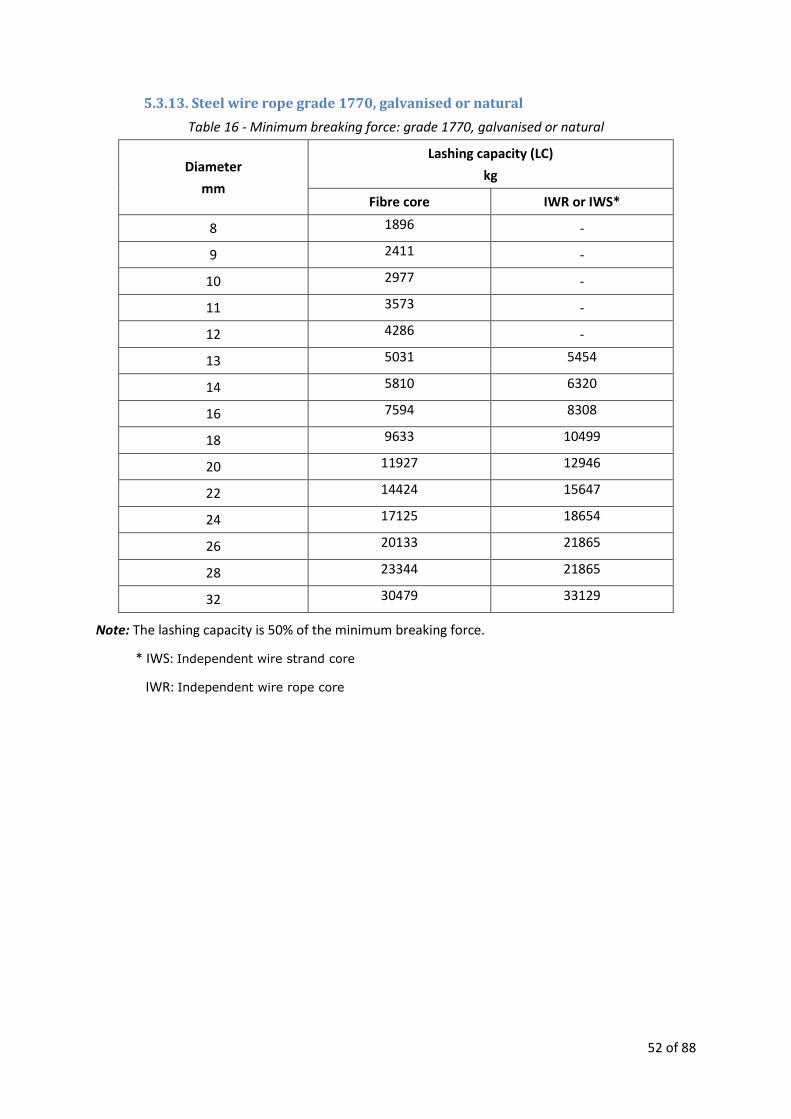
5.3.13. Steel wire rope grade 1770, galvanised or natural

Table 16 - Minimum breaking force: grade 1770, galvanised or natural

Diameter

mm


kg

Fibre core IWR or IWS*

8 1896 -

9 2411 -

10 2977 -

11 3573 -

12 4286 -

13 5031 5454

14 5810 6320

16 7594 8308

18 9633 10499

20 11927 12946

22 14424 15647

24 17125 18654

26 20133 21865

28 23344 21865

32 30479 33129


* IWS: Independent wire strand core

IWR: Independent wire rope core

53 of 88

6. Working Load Limits for Unrated Equipment Used for Load

Restraining

6.1. Chains

Size (mm) Grade 30 proof coil

Grade 43 High test

Grade 70 Transport Grade 80 Alloy

Grade 100 Alloy

7mm 580 kg 1180 kg 1430 kg 1570 kg 1950 kg

8mm 860 kg 1770 kg 2130 kg 2000 kg 2600 kg

10mm 1200 kg 2450 kg 2990 kg 3200 kg 4000 kg

11 mm 1680 kg 3270 kg 3970 kg - -

13mm 2030 kg 4170 kg 5130 kg 5440 kg 6800 kg

16mm 3130 kg 5910 kg 7170 kg 8200 kg 10300 kg

6.2. Manila Rope

Diameter Lashing Capacity

10 mm 90 kg

11 mm 120 kg

13 mm 150 kg

16 mm 210 kg

20 mm 290 kg

25 mm 480 kg

6.3. Wide Rope (6x37, Fibre Core)


7 mm 640 kg

8 mm 950 kg

10 mm 1360 kg

11 mm 1860 kg

13 mm 2400 kg

16 mm 3770 kg

20 mm 4940 kg

22 mm 7300 kg

25 mm 9480 kg

54 of 88

6.4. Steel Strapping

WidthxThinckness Lashing Capacity

31.7x0.74 mm 90 kg

31.7x0.79 mm 120 kg

31.7x0.89 mm 150 kg

31.7x1.12 mm 210 kg

31.7x1.27 mm 290 kg

31.7x1.5 mm 480 kg

50.8x1.12 mm 1200 kg

50.8x1.27 mm 1200 kg

6.5. Synthetic Webbing

Width Lashing Capacity

45 mm 790 kg

50 mm 910 kg

75 mm 1360 kg

100 mm 1810 kg

6.6. Polypropylene Fibre Rope (3&8 Strand Construction)


10 mm 180 kg

11 mm 240 kg

13 mm 280 kg

16 mm 420 kg

20 mm 580 kg

25 mm 950 kg

55 of 88

6.7. Polyester Fibre Rope (3&8 Strand Construction)


10 mm 250 kg

11 mm 340 kg

13 mm 440 kg

16 mm 680 kg

20 mm 850 kg

25 mm 1500 kg

6.8. Nylon Rope


10 mm 130 kg

11 mm 190 kg

13 mm 240 kg

16 mm 420 kg

20 mm 640 kg

25 mm 1140 kg

6.9. Double Braided Nylon Rope


10 mm 150 kg

11 mm 230 kg

13 mm 300 kg

16 mm 510 kg

20 mm 830 kg

25 mm 1470 kg

56 of 88

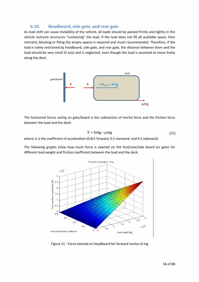
6.10. Headboard, side gate, and rear gate As load shift can cause instability of the vehicle, all loads should be packed firmly and tightly in the

vehicle restraint structures “containing” the load. If the load does not fill all available space, then

restraint, blocking or filling the empty spaces is required and much recommended. Therefore, if the

load is solely restrained by headboard, side gate, and rear gate, the distance between them and the

load should be very small (if any) and is neglected, even though the load is assumed to move freely

along the deck.

The horizontal forces acting on gate/board is the subtraction of inertia force and the friction force

between the load and the deck:

mgkmgF (25)

where, k is the coefficient of acceleration (0.8/1 forward, 0.5 rearward, and 0.5 sideward)

The following graphs show how much force is exerted on the font/rear/side board (or gate) for

different load weight and friction coefficient between the load and the deck.

Figure 51 - Force exerted on headboard for forward inertia of mg

mamax = kmg

μmg

gate/board

load

F F

57 of 88

Figure 52 - Force exerted on headboard for forward inertia of 0.8mg

Figure 53 - Force exerted on side/rear gate (inertia of 0.5mg)

In the case where the friction contact between the load and the deck is broken (due to going over

bumps), μ is considered to be zero. The force will be:

kmgF (26)

Figures 54-56 illustrate the force determined by Equation (26).

58 of 88

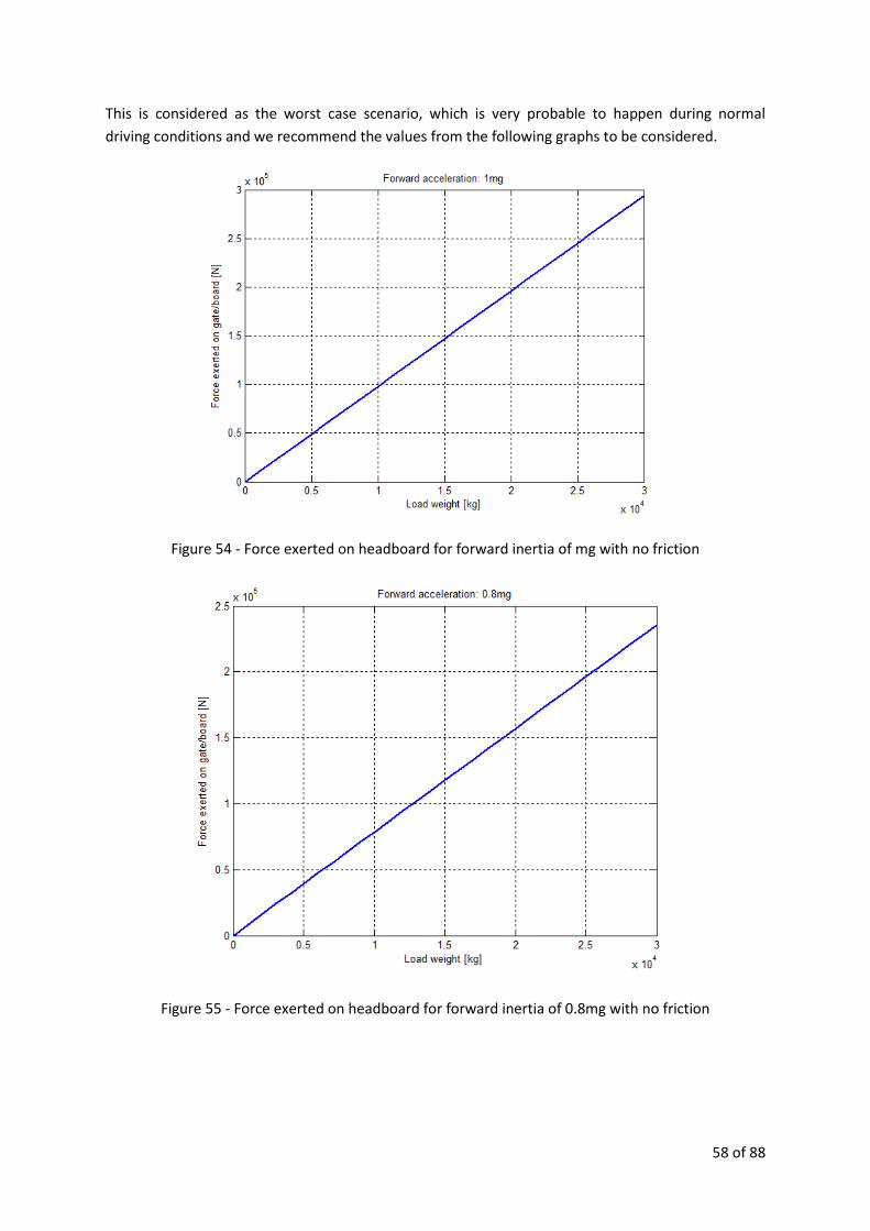
This is considered as the worst case scenario, which is very probable to happen during normal

driving conditions and we recommend the values from the following graphs to be considered.

Figure 54 - Force exerted on headboard for forward inertia of mg with no friction

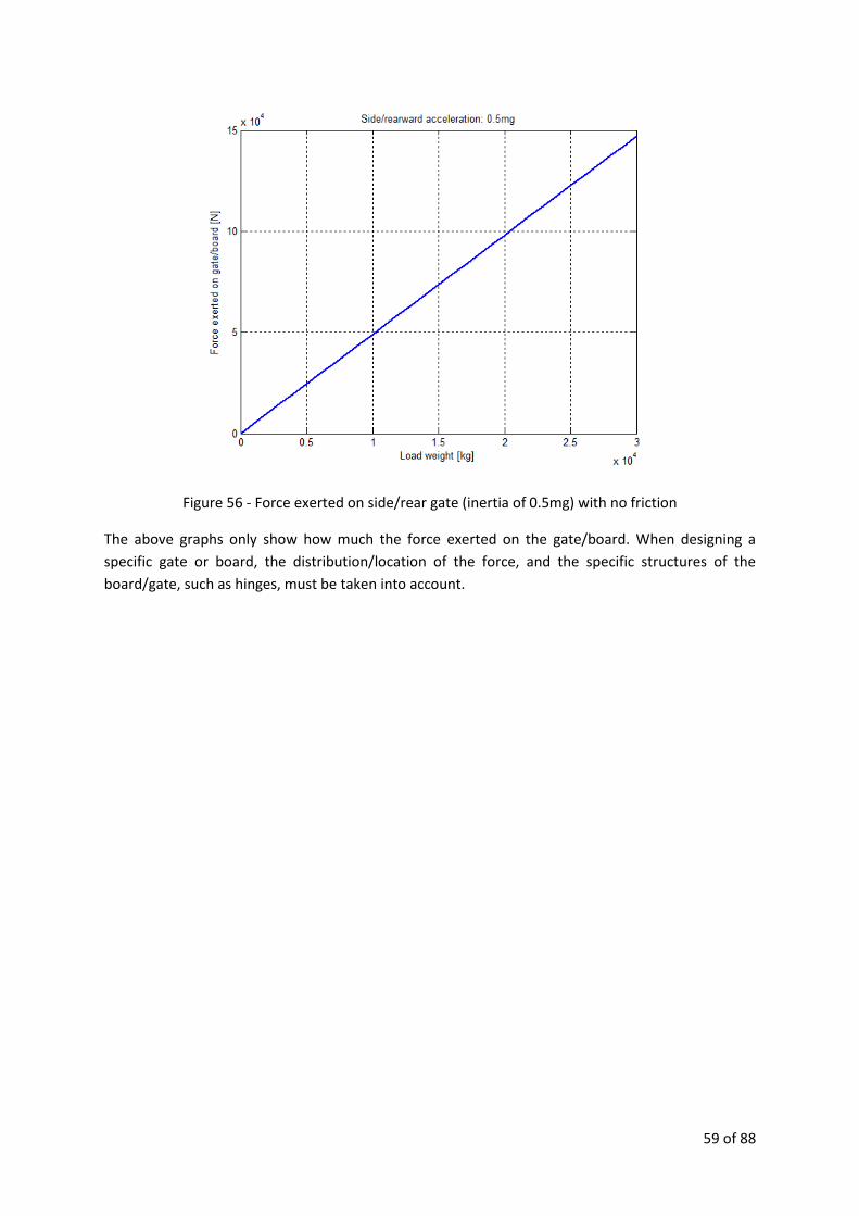
Figure 55 - Force exerted on headboard for forward inertia of 0.8mg with no friction

59 of 88

Figure 56 - Force exerted on side/rear gate (inertia of 0.5mg) with no friction

The above graphs only show how much the force exerted on the gate/board. When designing a

specific gate or board, the distribution/location of the force, and the specific structures of the

board/gate, such as hinges, must be taken into account.

60 of 88

7. Effect of Wear on Road Restraint Equipment

The lashing capacity of particular restraint equipment is proportional to its breaking force:

bsFkLC (25)

where, LC is the lashing capacity of the equipment, Fb presents the breaking force of the equipment,

ks is the safety factor (ks = 1/3 for rope, k = ½ for chain)

The rest of the details including the relationship between the breaking force and diameter and

lashing capacity calculations are available in the appendix A.

The results show that only 5% reduction of the width or diameter of restraint equipment will make

the use of the equipment risky. It is recommended that the width or diameter of the damaged

section be measured prior to use. The values can be used based in the equation below to assure the

health of the equipment.

𝐴𝑙𝑙𝑜𝑤𝑒𝑑 𝑑𝑎𝑚𝑎𝑔𝑒 𝑣𝑎𝑙𝑢𝑒 = 100 − (𝐷𝑖𝑎𝑚𝑒𝑡𝑒𝑟 𝑜𝑟 𝑤𝑖𝑑𝑡ℎ𝑠 𝑜𝑓 𝑡ℎ𝑒 𝑑𝑎𝑚𝑎𝑔𝑒𝑑 𝑠𝑒𝑐𝑡𝑖𝑜𝑛

𝑂𝑟𝑖𝑔𝑖𝑛𝑎𝑙 𝑑𝑖𝑎𝑚𝑒𝑡𝑒𝑟 𝑜𝑟 𝑤𝑖𝑑𝑡ℎ𝑋100) (26)

The value calculated above should not be above 5. Replacement of the restraint equipment is

recommended for Allowed damage values bigger than 5.

61 of 88

8. Appendix A In this appendix the calculations, formulations and equations used as a proof or to prove concepts

which are used in the context of the report are mentioned. It has been tried to write the report and

appendixes as individual pieces. Some materials might be repeated from the report as a result.

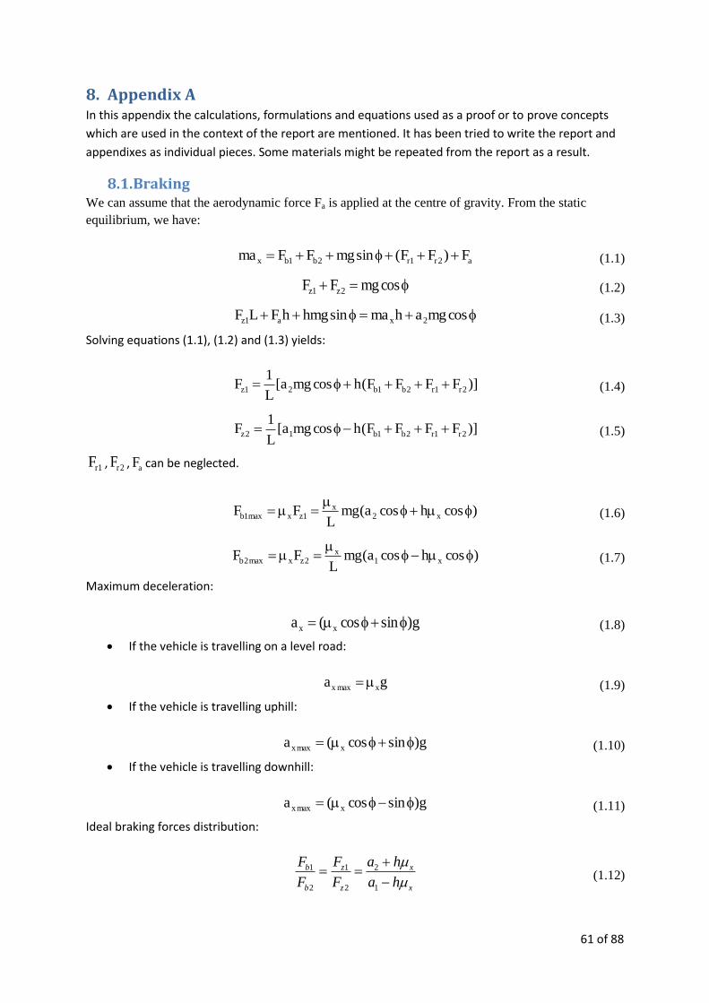
8.1. Braking We can assume that the aerodynamic force Fa is applied at the centre of gravity. From the static

equilibrium, we have:

a2r1r2b1bx F)FF(sinmgFFma (1.1)

cosmgFF 2z1z

(1.2)

cosmgahmasinhmghFLF 2xa1z (1.3)

Solving equations (1.1), (1.2) and (1.3) yields:

)]FFFF(hcosmga[L

1F 2r1r2b1b21z (1.4)

)]FFFF(hcosmga[L

1F 2r1r2b1b12z

(1.5)

1rF , 2rF , aF can be neglected.

)coshcosa(mgL

FF x2x

1zxmax1b

(1.6)

)coshcosa(mgL

FF x1x

2zxmax2b

(1.7)

Maximum deceleration:

g)sincos(a xx (1.8)

If the vehicle is travelling on a level road:

ga xmaxx (1.9)

If the vehicle is travelling uphill:

g)sincos(a xmaxx (1.10)

If the vehicle is travelling downhill:


Ideal braking forces distribution:

x

x

z

z

b

b

ha

ha

F

F

F

F

1

2

2

1

2

1 (1.12)

62 of 88

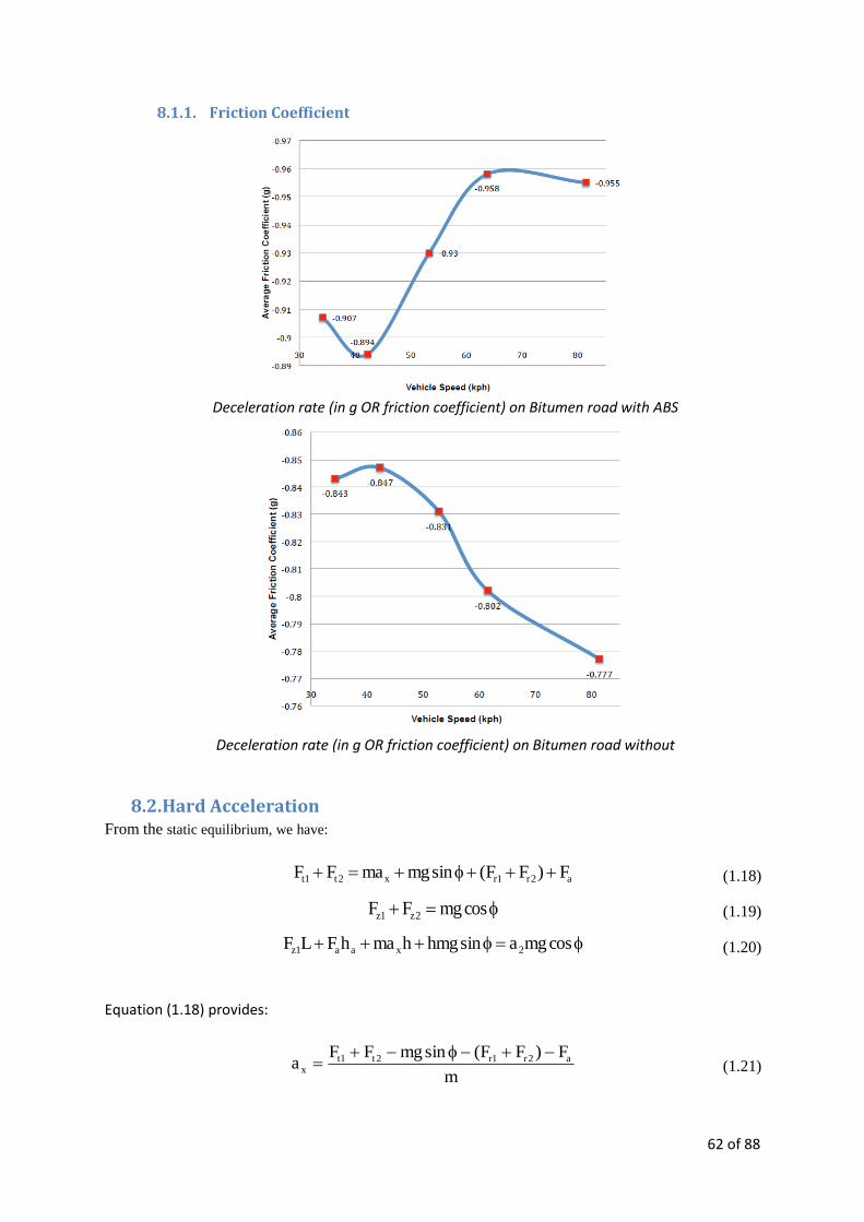
8.1.1. Friction Coefficient

Deceleration rate (in g OR friction coefficient) on Bitumen road with ABS

Deceleration rate (in g OR friction coefficient) on Bitumen road without

8.2. Hard Acceleration From the static equilibrium, we have:

a2r1rx2t1t F)FF(sinmgmaFF (1.18)

cosmgFF 2z1z (1.19)

cosmgasinhmghmahFLF 2xaa1z (1.20)

Equation (1.18) provides:

m

F)FF(sinmgFFa a2r1r2t1t

x

(1.21)

63 of 88

Maximum acceleration: the maximum acceleration of the vehicle can be achieved when the tires

reach their maximum traction potentials at the same time:

1zxmax1t FF ; 2zxmax2t FF (1.22)

From (1.19), (1.21), and (1.22) we have:

m

F)FF(sinmgcosmga a2r1rx

x

(1.23)

As max2tmax1ta2r1r FFFFF

(1.23) becomes:

g)sincos(a xmaxxf (1.24)

If the vehicle is travelling on a level road:

ga xmaxx (1.25)

If the vehicle is travelling uphill:


If the vehicle is travelling downhill:


8.2.1. Power limited acceleration

The Newton’s Second Law read:

xxxxe vma1

vF1

P

(1.28)

or x

ex

v

1

m

Pa

(1.29)

where η is the efficiency of the vehicle. If Pe = PM, the maximum acceleration will be:

x

Mmaxx

v

1

m

Pa (1.30)

With a rarely very high power to weight ratio of 54.22 W/kg for truck (Ahanotu, 1999), and a high

efficiency of 0.9, (1.30) becomes:

xx

maxxv

8.48

v

1 x 22.54 x 9.0a (1.31)

If the vehicle is traveling with vx > 10 m/s (36 km/h), the maximum acceleration will be:

64 of 88

0.5g ][m/s 88.410

8.48a 2

maxx (1.32)

Therefore, a maximum forward acceleration that higher than 0.5g may only occur at velocity less

than 10 m/s.

8.2.2. Transmission System

The torque delivered through the clutch as input to the transmission is:

eeec ITT (1.33)

where:

Tc is torque at the clutch as the input to the transmission

Te is engine torque at a given speed

Ie is engine rotational inertia

αe is engine rotational acceleration

Similarly, the torque delivered at the output of the transmission is:

tetcd i)IT(T (1.34)

where:

Td is torque at the driveshaft

It is rotational inertia of transmission as seen from the engine side

it is ratio of the transmission

The torque as the input to the axles to accelerate rotating wheels and provide traction at the ground

is:

wwtfddda IrFi)IT(T (1.35)

where:

Ta is torque on the axles

Id is rotational inertia of the driveshaft

αa is driveshaft rotational acceleration

if is ratio of the final drive

Ft is tractive force at the ground

Iw is the rotational of the wheels and axles shafts

αw is the rotational acceleration of the wheels

65 of 88

r is the wheels radius

The above rotational accelerations are related to each other as the following:

wftdtewfd iii;i (1.36)

From (1.33) to (1.36), with the inefficiencies due to mechanical and viscous losses in the driveline

components taken into account, we have:

2

xw

2

fd

2

f

2

ttetffte

tr

a]IiIii)II[(ii

r

TF (1.37)

From (1.18), we have:

a2r1rtx F)FF(sinmgFma (1.38)

Substituting (1.37) in (1.38) yields:

a2r1r2

xw

2

fd

2

f

2

ttetffte

x F)FF(sinmgr

a]IiIii)II[(ii

r

Tma (1.39)

or

a2r1rtffte

x2w

2

fd

2

f

2

tte F)FF(sinmgiir

Ta}

r

1]IiIii)II[(m{ (1.40)

The rotational inertia terms are usually lumped in with the mass of the vehicle, so the simplified

equation will be:

a2r1rtffte

xr F)FF(sinmgiir

Ta)mm( (1.41)

where,

mr is the equivalent mass of the rotating components.

The combination of the two masses is an “effective mass”, and the ratio of (m+mr)/m is “mass

factor”. The mass factor of a vehicle will depend on the operating gear (Gillespie, 1995) :

2

f

2

t i0.0025i0.04 1 factor mass (1.42)

If all the resistance forces are neglected, (1.41) will be written as:

xr

Mtfx

v

1

mm

Pa

(1.43)

(1.43) shows that, the acceleration is far less than that calculated from (1.30). Therefore, the

theoretical acceleration of 0.5g may only occur at low speed even far less than 10 m/s.

66 of 88

8.3. Dynamics of a Turning Vehicle The Newton-Euler equations of motion for a rigid vehicle in the body coordinate frame B, which is

the frame attached to the vehicle at its centre of gravity C, are:

yxx mrvvmF (1.51)

xyy mrvvmF (1.52)

zz IrM (1.53)

where, vx, vy, are longitudinal, lateral velocity of the vehicle centre expressed in the body coordinate

frame, r is the yaw rate of the vehicle ,m presents the weight of the vehicle, Iz is the rotational inertia

of the vehicle about Cz.

The force system acting on the vehicle includes:

4x3x22y11yx FFsinFsinFF (1.54)

4y3y22y11yy FFcosFcosFF (1.55)

)FF(b)FFsinFsinF(2

w)cosFcosF(a)MMMM(M 4y3y4x3x22y11y22y11y4z3z2z1zz (1.56)

Coupling (1.51), (1.52), (1.53) with (1.54), (1.55), (1.56) yields the equations of motion of the turning

vehicle:

y4x3x22y11yx rv)FFsinFsinF(m

1v (1.57)

x4y3y22y11yy rv)FFcosFcosF(m

1v (1.58)

)]FF(b)FFsinFsinF(2

w)cosFcosF(a)MMMM([

I

1r 4y3y4x3x22y11y22y11y4z3z2z1z

z

(1.59)

In order to take the non-linearity characteristics of the tyre into consideration, the Magic Formula is utilised

for tyre modelling.

),F(FF iziyiyi (1.60)

),F(MM izizizi (1.61)

where,

Fzi presents vertical load under the tyre number i

αi is side slip of the tyre number i

During cornering manoeuvre, load is transferring laterally and longitudinally. These effects are

modelled as the following equations:

y

g

x

g

1z awL

mbha

L2

mh

L2

mgbF (1.62)

67 of 88

y

g

x

g

1z awL

mbha

L2

mh

L2

mgbF (1.63)

y

g

x

g

1z awL

mbha

L2

mh

L2

mgbF

(1.64)

y

g

x

g

1z awL

mbha

L2

mh

L2

mgbF

(1.65)

The side slip angle relate to the motion of the vehicle as the following equations:

r

2

wv

arvtan

x

y1

11

(1.66)

r

2

wv

arvtan

x

y1

22

(1.67)

r

2

wv

brvtan

x

y1

3

(1.68)

r

2

wv

brvtan

x

y1

4

(1.69)

The equations of motion are modelled in Simulink environment, as shown in Figure:

Dynamic model of a turning vehicle built in Simulink environment

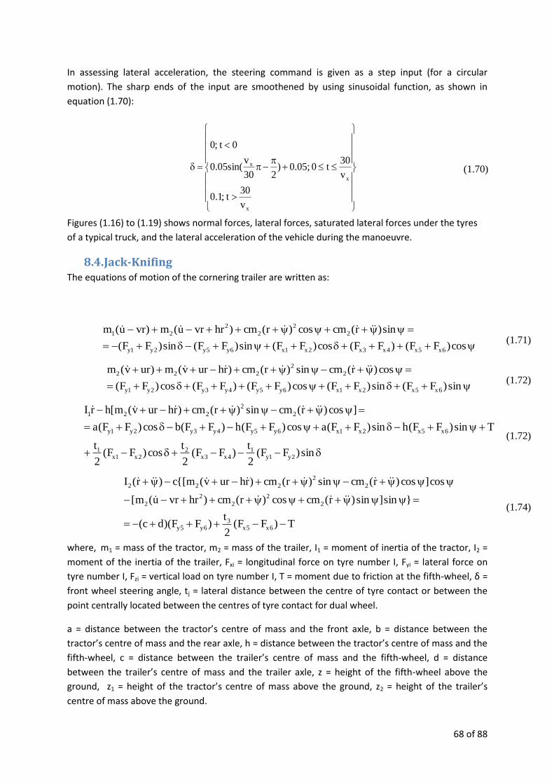
68 of 88

In assessing lateral acceleration, the steering command is given as a step input (for a circular

motion). The sharp ends of the input are smoothened by using sinusoidal function, as shown in

equation (1.70):

x

x

x

v

30 t;1.0

v

30t0 0.05;)

230

v0.05sin(

0 t;0

(1.70)

Figures (1.16) to (1.19) shows normal forces, lateral forces, saturated lateral forces under the tyres

of a typical truck, and the lateral acceleration of the vehicle during the manoeuvre.

8.4. Jack-Knifing The equations of motion of the cornering trailer are written as:

cos)FF()FF(cos)FF(sin)FF(sin)FF(

sin)r(cmcos)r(cm)hrvru(m)vru(m

6x5x4x3x2x1x6y5y2y1y

2

2

2

2

21

(1.71)

sin)FF(sin)FF(cos)FF()FF(cos)FF(

cos)r(cmsin)r(cm)rhurv(m)urv(m

6x5x2x1x6y5y4y3y2y1y

2

2

222

(1.72)

sin)FF(2

t)FF(

2

tcos)FF(

2

t

Tsin)FF(hsin)FF(acos)FF(h)FF(bcos)FF(a

]cos)r(cmsin)r(cm)rhurv(m[hrI

2y1y1

4x3x2

2x1x1

6x5x2x1x6y5y4y3y2y1y

2

2

221

(1.72)

T)FF(2

t)FF)(dc(

}sin]sin)r(cmcos)r(cm)hrvru(m[

cos]cos)r(cmsin)r(cm)rhurv(m{[c)r(I

6x5x3

6y5y

2

2

2

2

2

2

2

222

(1.74)

where, m1 = mass of the tractor, m2 = mass of the trailer, I1 = moment of inertia of the tractor, I2 =

moment of the inertia of the trailer, Fxi = longitudinal force on tyre number I, Fyi = lateral force on

tyre number I, Fzi = vertical load on tyre number I, T = moment due to friction at the fifth-wheel, δ =

front wheel steering angle, tj = lateral distance between the centre of tyre contact or between the

point centrally located between the centres of tyre contact for dual wheel.

a = distance between the tractor’s centre of mass and the front axle, b = distance between the

tractor’s centre of mass and the rear axle, h = distance between the tractor’s centre of mass and the

fifth-wheel, c = distance between the trailer’s centre of mass and the fifth-wheel, d = distance

between the trailer’s centre of mass and the trailer axle, z = height of the fifth-wheel above the

ground, z1 = height of the tractor’s centre of mass above the ground, z2 = height of the trailer’s

centre of mass above the ground.

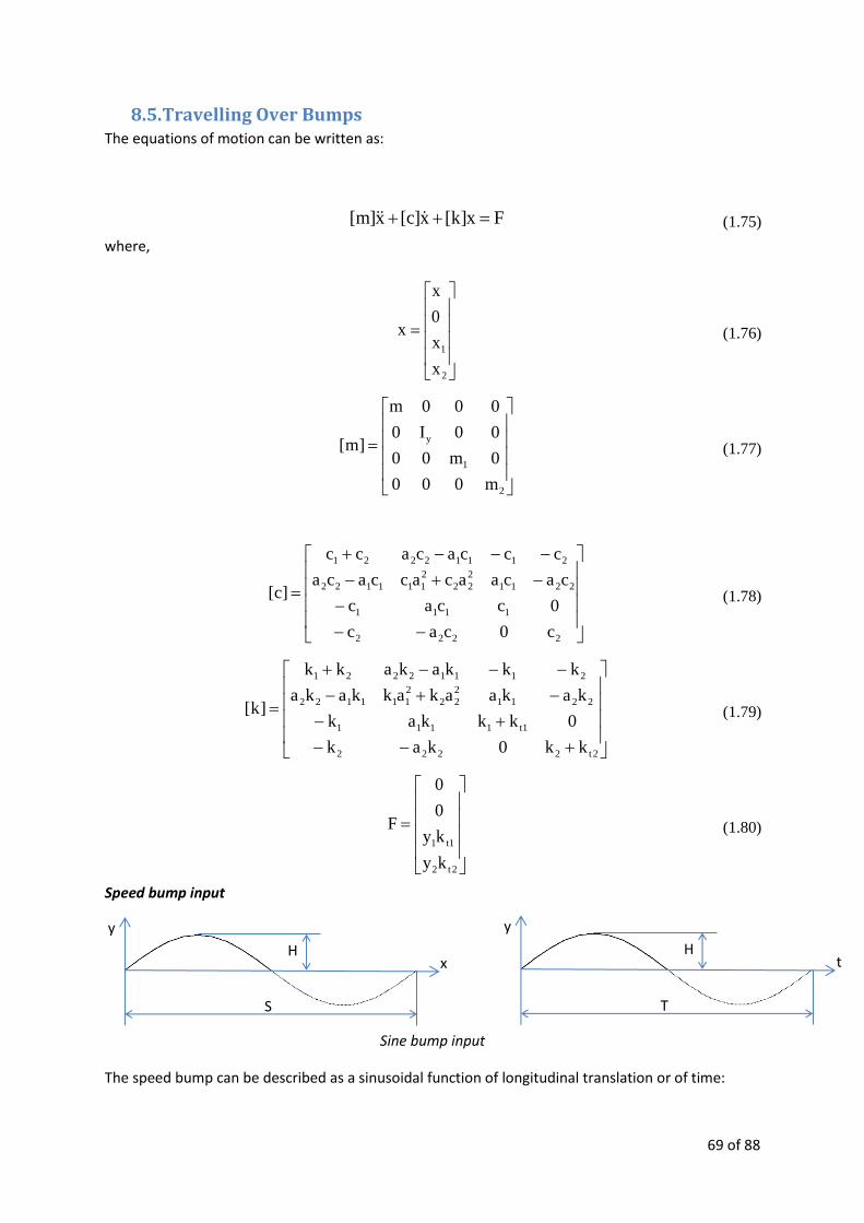
69 of 88

8.5. Travelling Over Bumps The equations of motion can be written as:

Fx]k[x]c[x]m[ (1.75)

where,

2

1

x

x

0

x

x (1.76)

2

1

y

m000

0m00

00I0

000m

]m[ (1.77)

2222

1111

2211

2

22

2

111122

21112221

c0cac

0ccac

cacaacaccaca

cccacacc

]c[ (1.78)

2t2222

1t1111

2211

2

22

2

111122

21112221

kk0kak

0kkkak

kakaakakkaka

kkkakakk

]k[ (1.79)

2t2

1t1

ky

ky

0

0

F (1.80)

Speed bump input

Sine bump input

The speed bump can be described as a sinusoidal function of longitudinal translation or of time:

H x

y

S

H t

y

T

70 of 88

xS

2sinH)x(y

(1.81)

vtS

2sinHt

T

2sinH)t(y

(1.82)

If the front excitation input is determined by:

vtS

2sinH)t(y1

(1.83)

Then, then rear excitation input will be:

)v

Lt(v

S

2sinH)t(y2

(1.84)

where, L is the wheelbase of the vehicle.

8.6. Minor Collision

The Newton’s law of restitution states that:

101012 eIII (1.86)

or

1012 I)1e(I (1.87)

where, e is called the coefficient of restitution. The law can also be expressed as:

12 epp (1.88)

The Newton’s law equation (1.88), coupled with momentum equation (1.85) are sufficient to

determine the final velocities of the two vehicles.

Applying parameters at the instant t2 to (1.84), and rewriting (1.87) yields:

2121 mvImv (1.89)

2121 MVIMV (1.90)

)vV(evV 1122 (1.91)

Solving the three equations system provides:

)vV)(e1(

M

m1

1vvv 1121

(1.92)

71 of 88

)vV)(e1(

1m

M

1VVV 1121

(1.93)

The vehicle B with mass m travelling at 30 km/h, and collides with the car A with a mass M moving

at the same speed.

)e1(

M

m1

67.16)

6.3

30

6.3

30)(e1(

M

m1

1vvv 21

(1.94)

Let us determine the Δv of the vehicle B for 0 ≤ e ≤ 1, and 0.1m ≤ m ≤ 10M

As the real impact practically lasts for about 1/10 second (Macmillan, 1983), in this estimation we

assume that Δt = t2 – t1 = 0.1 (s). Therefore, the average deceleration that the vehicle B experiences

is:

)1(

1

7.166. e

M

mt

va crashx

(1.95)

The average deceleration rate of the vehicle B is illustrated in Figure 1.28 with the minimum value of

15.15 m/s2 associated with e = 0 (totally inelastic) and m/M = 10;

As a fixed block is expressed as 0V ;M 1 , (1.92) becomes:

6.3

30)e1(v)e1(v 1 (1.96)

Therefore, the average deceleration is:

)(m/s 3.833.83)e1(t

va 2

crash.x

(1.97)

The vehicles A and B (masses are m and M) moving at the same speed v.

)1(

1

5556.0)

6.36.3)(1(

1

121 e

M

m

vvve

M

mvvv

(1.98)

The average deceleration that the vehicle B experiences will be:

81.9 8.08.0)1(

1

556.5. xge

M

m

v

t

va crashx

(1.99)

or

72 of 88

)1()1(

4125.1

M

m

ev

(1.100)

Vehicle B with mass m travelling at v (km/h) collides with a fixed block.

1)1( vev (1.101)

Therefore, the average deceleration is:

9.81 x 0.8 0.8g )1(10 1.

ve

t

va crashx (1.102)

or

e1

0.7848 1

v (1.103)

8.7. Tie-Down Lashing

8.7.1. Symmetry

The clamping force Fc must satisfy:

Sliding balance:

k*W ≤ μ(W + Fc) (2.1)

Tipping balance:

h*k*W ≤ b(W + Fc) (2.2)

The tensioning force needed (one lashing) to safely restraint load on the vehicle is now written as:

Sliding balance:

k*W + ≤ μ[W + 2FTsinα] (2.3)

Tipping balance:

h*k*W ≤ b*W + 2b*FTsinα (2.4)

And, maximum weight each lashing can safely restraint is:

Sliding balance:

k

sinF2W T

for k > μ (2.5)

If k ≤ μ, (2.3) is always satisfied. However, the tie-down lashings must be pre-tensioned to provide a

minimum clamping force of 20% of the weight of the load. This is because the load must always

remain in contact with the deck during road vibration and over bumps to maintain the friction force

during normal driving. To meet the requirement, the maximum weight can be determined by the

following:

73 of 88

W ≤ 10FTsinα for k ≤ μ (2.6)

Tipping balance:

bhk

sinbF2W T

for hk > b (2.7)

W ≤ 10FTsinα for hk ≤ b (2.8)

8.7.2. Asymmetry

The tensioning force needed, in the worst case, to safely restraint load on the vehicle is now written

as:

Sliding balance:

k*W + FT(1 -c2)cosα ≤ μ[W + FT(1 +c

2)sinα] (2.9)

Tipping balance:

h*k*W + 2h* FT(1 -c2)cosα ≤ b*W + 2b*c

2FTsinα (2.10)

And, maximum weight each lashing can safely restraint is:

Sliding balance:

k

]cos)1c(sin)c1([FW

22

T for k > μ (2.11)

W ≤ 5FT(1+c2)sinα for k ≤ μ (2.12)

Tipping balance:

bhk

]cos)1c(h2sinbc2[FW

22

T

for hk > b (2.13)

W ≤ 5FT(1+c2)sinα for k ≤ μ (2.14)

8.7.3. Safety Factor

cos)1c(sin)c1(

sin2

k

)]1c(sin)c1([F:

k

sinF2K

22

22

TTL (2.15)

or

cos)1e(sin)e1(

sin2K

'2'2L (2.16)

The maximum load weight that a particular lashing can safely restraint by (2.5), the real value should

be used as the following:

74 of 88

L

T

K)k(

sinF2W

(2.17)

or

k

sinFW T

max (2.18)

8.8. Direct Lashing The minimum strength required for each of n lashings directly restraining is:

kWcosnF minT (2.19)

or

cos

k

n

WF minT (2.20)

where, k is the coefficient of acceleration (0.8 forward, 0.5 rearward, and 0.5 sideward), n presents

the number of lashing , W is the weight of the load, α is the angle of the lashing with respect to the

direction of acceleration.

The minimum strength (lashing capacity) required for only one lashing to restrain 100 kg load with k

= 0.8, and k = 0.5. For this load configuration, the formula (2.20) becomes:

cos

k

1

100F minT (2.21)

8.9. Conditions Likely to Effect Better or Worse of the Safe Carriage of

Loads If the ratio of the front braking force to that of the rear is c, there is only a value of friction

coefficient that is fully utilised. That friction coefficient is determined by (3.1)

01

02

2

1

ha

ha

F

Fc

b

b

(3.1)

or

)1(

210

ch

aca (3.2)

If the friction coefficient is more than this value, μ1 > μ0, the rear wheels are locked before the front

braking force reaches its capacity.

The braking force at rear wheel will be:

)( 11

212 hagamL

FF zb

(3.3)

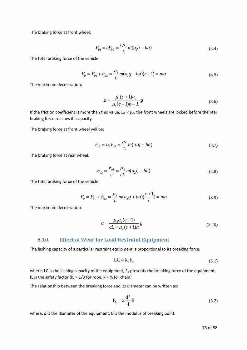
75 of 88

The braking force at front wheel:

)( 11

21 hagamL

ccFF bb

(3.4)

The total braking force of the vehicle:

machagamL

FFF bbb )1)(( 11

21

(3.5)

The maximum deceleration:

gLhc

aca

)1(

)1(

1

11

(3.6)

If the friction coefficient is more than this value, μ2 < μ0, the front wheels are locked before the rear

braking force reaches its capacity.

The braking force at front wheel will be:

)( 22

121 hagamL

FF zb

(3.7)

The braking force at rear wheel:

)( 221

2 hagamcLc

FF b

b

(3.8)

The total braking force of the vehicle:

mac

chagam

LFFF bbb

)

1)(( 2

221

(3.9)

The maximum deceleration:

ghccL

caa

)1(

)1(

2

22

(3.10)

8.10. Effect of Wear for Load Restraint Equipment

The lashing capacity of a particular restraint equipment is proportional to its breaking force:

bsFkLC (5.1)

where, LC is the lashing capacity of the equipment, Fb presents the breaking force of the equipment,

ks is the safety factor (ks = 1/3 for rope, k = ½ for chain)

The relationship between the breaking force and its diameter can be written as:

E4

dF

2

b (5.2)

where, d is the diameter of the equipment, E is the modulus of breaking point.

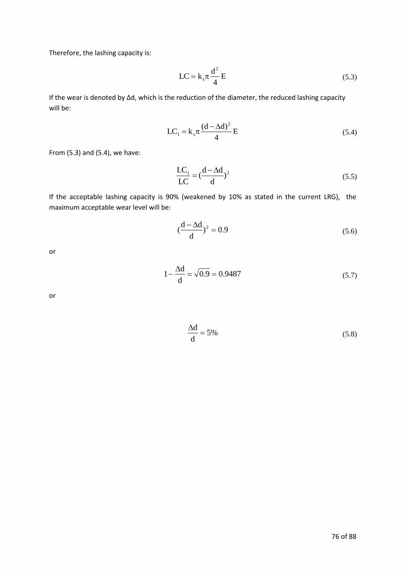
76 of 88

Therefore, the lashing capacity is:

E4

dkLC

2

s (5.3)

If the wear is denoted by Δd, which is the reduction of the diameter, the reduced lashing capacity

will be:

E4

)dd(kLC

2

s1

(5.4)

From (5.3) and (5.4), we have:

21 )

d

dd(

LC

LC (5.5)

If the acceptable lashing capacity is 90% (weakened by 10% as stated in the current LRG), the

maximum acceptable wear level will be:

9.0)d

dd( 2

(5.6)

or

9487.09.0d

d1

(5.7)

or

%5d

d

(5.8)

77 of 88

78 of 88

9. Appendix B

Lashing angle: sinE

Old New

Tie-down angle effect (page 189)

The curve provides any value of tie-down effect between 00 and 900 tie-down angle

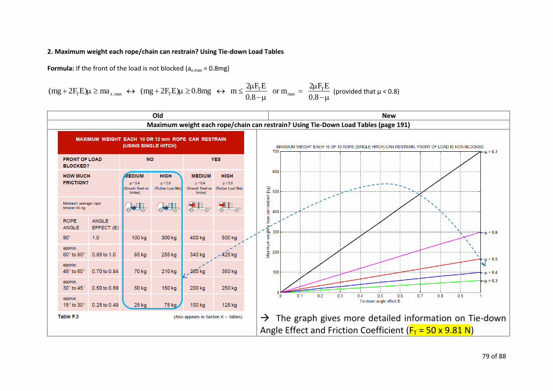
79 of 88

2. Maximum weight each rope/chain can restrain? Using Tie-down Load Tables

Formula: If the front of the load is not blocked (ax.max = 0.8mg)

8.0

EF2 mor

8.0

EF2m mg8.0 )EF2mg( ma)EF2mg( T

maxT

Tmax.xT (provided that μ < 0.8)

Old New

Maximum weight each rope/chain can restrain? Using Tie-Down Load Tables (page 191)

The graph gives more detailed information on Tie-down Angle Effect and Friction Coefficient (FT = 50 x 9.81 N)

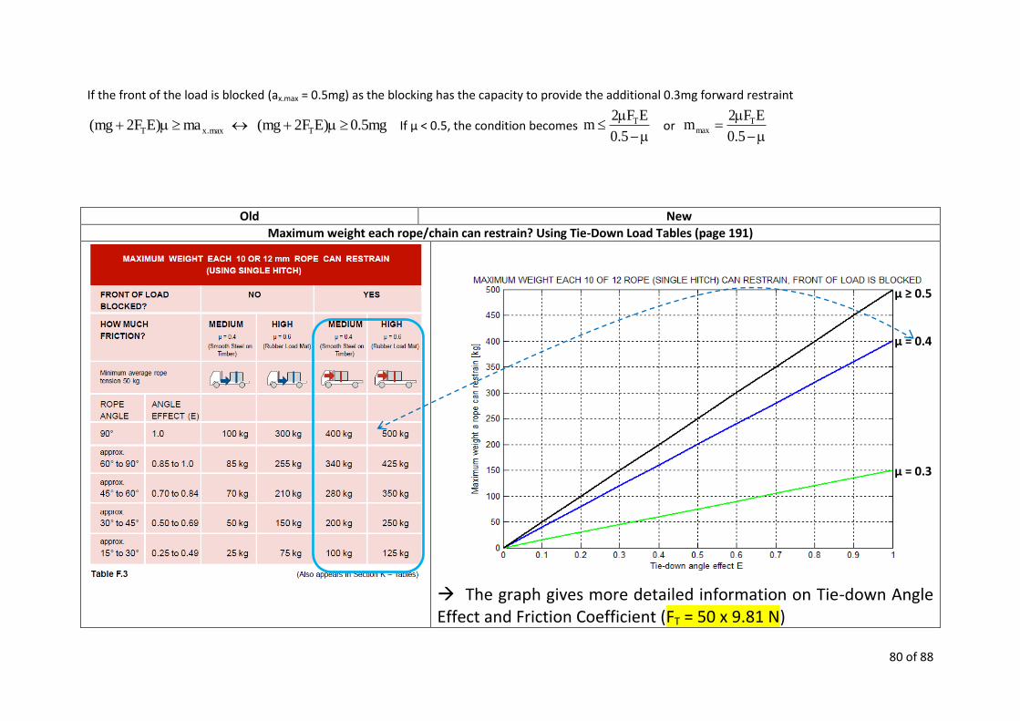
80 of 88

If the front of the load is blocked (ax.max = 0.5mg) as the blocking has the capacity to provide the additional 0.3mg forward restraint

mg5.0 )EF2mg( ma)EF2mg( Tmax.xT If μ < 0.5, the condition becomes 5.0

EF2m T

or

5.0

EF2m T

max

Old New



μ ≥ 0.5

μ = 0.4

μ = 0.3

81 of 88

If μ ≥ 0.5, the condition is always satisfied. However, as the minimum clamping force of 20% of the weight of the load is taken into account, we have:

g

EF10 m mg2.0EF2 T

T (black curve)

Old New



82 of 88

Old New



μ ≥ 0.5

μ = 0.4

μ = 0.3

83 of 88

Old New



84 of 88

Old New



μ = 0.3

μ = 0.4

μ ≥ 0.5

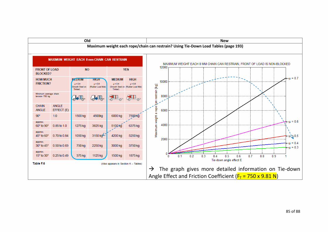
85 of 88

Old New



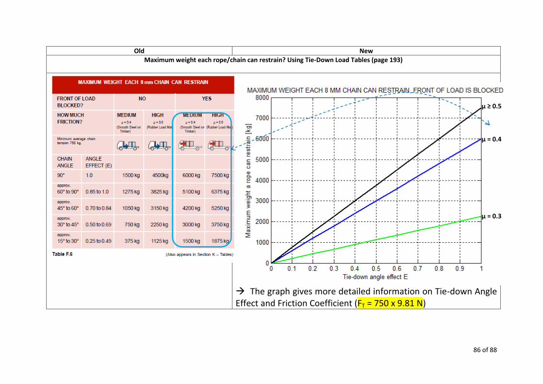
86 of 88

Old New



μ = 0.3

μ = 0.4

μ ≥ 0.5

87 of 88

3. Lashing angle: Formula: ii cosE

Old New

Tie-down angle effect (page 202)

The curve provides any value of direct lashing effect between 0

0 and 90

0 tie-down angle

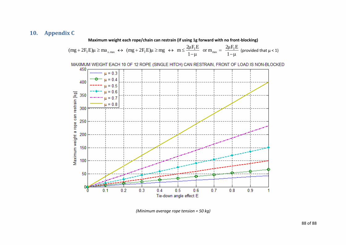
88 of 88

10. Appendix C Maximum weight each rope/chain can restrain (if using 1g forward with no front-blocking)

1

EF2 mor

1

EF2m mg )EF2mg( ma)EF2mg( T

maxT

Tmax.xT (provided that μ < 1)

(Minimum average rope tension = 50 kg)

89 of 88

Minimum average rope tension = 100 kg

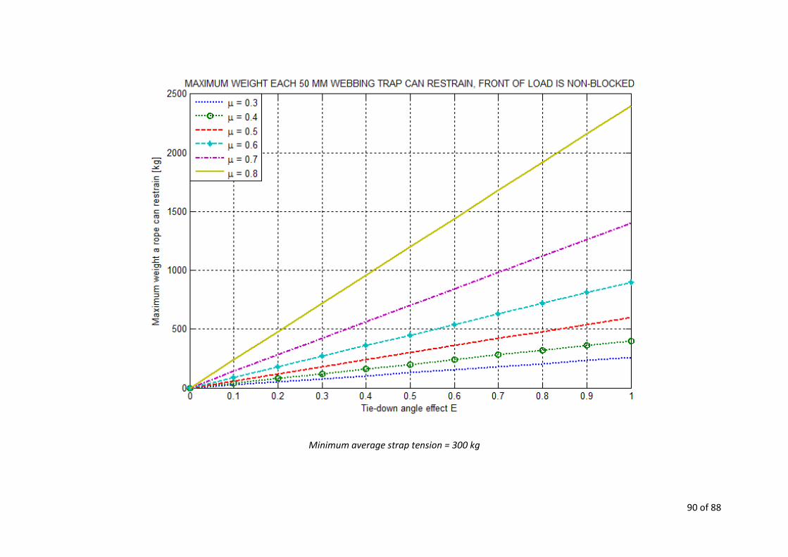
90 of 88

Minimum average strap tension = 300 kg

91 of 88

Minimum average chain tension = 750 kg

92 of 88

11. REFERENCES AHANOTU, D. N. 1999. Heavy-duty vehicle weight and horsepower distributions: measurement of class-specific

temporal and spatial variability. Georgia Institute of Technology. BOUTELDJA, M., KOITA, A., DOLCEMSACOLO, V. & CADIOU, J. C. Prediction and Detection of Jackknifing Problems

for Tractor Semi-Trailer. GILLESPIE, T. D. 1995. Fundamentals of vehicle dynamics. Warrendale, Pa: Society of Automotive Engineers. HARTMAN, J. 2014. Effects of velocity, temperature and rainfall on the friction coefficient of pneumatic tyres and

bitumen roads. RMIT University. HARWOOD, D. W., PROGRAM, N. C. H. R. & BOARD, N. R. C. T. R. 2003. Review of Truck Characteristics as Factors

in Roadway Design, Transportation Research Board, National Research Council. LONG, G. 2000. Acceleration Characteristics of Starting Vehicles. Transportation Research Record, 1737, 58-70. MACMILLAN, R. H. 1983. Dynamics of vehicle collisions, St. Helier, Interscience Enterprises. MIKULCIK, E. C. 1971. The Dynamics of Tractor-Semitrailer Vehicles: The Jackknifing Problem. SAE International. PROCTOR, C. L., GRIMES, W. D., FOURNIER, D. J., RIGOL, J. & SUNSERI, M. G. 1995. Analysis of Acceleration in

Passenger Cars and Heavy Trucks. SAE International. WONG, J. Y. 2001. Theory of ground vehicles, John Wiley & Sons.

http://ntc.gov.au/Media/Reports/(E62BE286-4870-ED95-1914-1A70F3250782).pdf

Driver's Handbook on Cargo Securment ; A guide to North American Cargo Securment Standards

ttps://www.fmcsa.dot.gov/sites/fmcsa.dot.gov/files/docs/Drivers_Handbook_Cargo_Securement.pdf

1. - NTC - National Transport Commission7114C62D-15B5-4241-915A... · These forces are specified in the 2004 edition of the Load Restraint Guide published by the NTC and represent

Documents