arXiv:1111.5950v3 [cs.IT] 10 May 2013 1 Non-Linear Transformations of Gaussians and Gaussian-Mixtures with implications on Estimation and Information Theory Paolo Banelli, Member, IEEE Abstract This paper investigates the statistical properties of non-linear trasformations (NLT) of random vari- ables, in order to establish useful tools for estimation and information theory. Specifically, the paper focuses on linear regression analysis of the NLT output and derives sufficient general conditions to establish when the input-output regression coefficient is equal to the partial regression coefficient of the output with respect to a (additive) part of the input. A special case is represented by zero-mean Gaussian inputs, obtained as the sum of other zero-mean Gaussian random variables. The paper shows how this property can be generalized to the regression coefficient of non-linear transformations of Gaussian- mixtures. Due to its generality, and the wide use of Gaussians and Gaussian-mixtures to statistically model several phenomena, this theoretical framework can find applications in multiple disciplines, such as communication, estimation, and information theory, when part of the nonlinear transformation input is the quantity of interest and the other part is the noise. In particular, the paper shows how the said properties can be exploited to simplify closed-form computation of the signal-to-noise ratio (SNR), the estimation mean-squared error (MSE), and bounds on the mutual information in additive non-Gaussian (possibly non-linear) channels, also establishing relationships among them. Index Terms Gaussian random variables, Gaussian-mixtures, non-linearity, linear regression, SNR, MSE, mutual information. The author is with the Department of Electronic and Information Engineering, University of Perugia, 06125 Perugia, Italy (e-mail: [email protected]). May 13, 2013 DRAFT

Welcome message from author
This document is posted to help you gain knowledge. Please leave a comment to let me know what you think about it! Share it to your friends and learn new things together.
Transcript
arX
iv:1
111.
5950
v3 [
cs.IT
] 10
May
201
31
Non-Linear Transformations of Gaussians and
Gaussian-Mixtures with implications on
Estimation and Information TheoryPaolo Banelli,Member, IEEE
Abstract
This paper investigates the statistical properties of non-linear trasformations (NLT) of random vari-
ables, in order to establish useful tools for estimation andinformation theory. Specifically, the paper
focuses on linear regression analysis of the NLT output and derives sufficient general conditions to
establish when the input-output regression coefficient is equal to thepartial regression coefficient of the
output with respect to a (additive) part of the input. A special case is represented by zero-mean Gaussian
inputs, obtained as the sum of other zero-mean Gaussian random variables. The paper shows how this
property can be generalized to the regression coefficient ofnon-linear transformations of Gaussian-
mixtures. Due to its generality, and the wide use of Gaussians and Gaussian-mixtures to statistically
model several phenomena, this theoretical framework can find applications in multiple disciplines, such
as communication, estimation, and information theory, when part of the nonlinear transformation input
is the quantity of interest and the other part is the noise. Inparticular, the paper shows how the said
properties can be exploited to simplify closed-form computation of the signal-to-noise ratio (SNR), the
estimation mean-squared error (MSE), and bounds on the mutual information in additive non-Gaussian
(possibly non-linear) channels, also establishing relationships among them.
Index Terms
Gaussian random variables, Gaussian-mixtures, non-linearity, linear regression, SNR, MSE, mutual
information.
The author is with the Department of Electronic and Information Engineering, University of Perugia, 06125 Perugia, Italy
(e-mail: [email protected]).
May 13, 2013 DRAFT
2
I. INTRODUCTION
Non-linear transformations (NLT) of Gaussian random variables, and processes, is a classical subject
of probability theory, with particular emphasis in communication systems. Several results are available
in the literature to statistically characterize the non-linear transformation output, for both real [1]–[8] and
complex [9]–[11] Gaussian-distributed input processes.
If the input to the non-linear transformation is the sum of two, or more, Gaussian random variables,
then the overall input is still Gaussian and, consequently,the statistical characterization can still exploit
the wide classical literature on the subject. For instance,a key point is to establish the equivalent input-
output linear-gain [or linear regression coefficient (LRC)] of the non linearity. Anyway, if the interest is
to infer only a part of the input by the overall output, and to establish apartial LRC (or linear-gain)
with respect to this part of the input, it is necessary to compute multiple-folded integrals involving the
non-linear transformation. This task is in general tediousand, sometimes, also prohibitive.
This paper observes that, if the NLT input is the sum of zero-mean, independent, Gaussian random
variables, all thepartial LRCs are identical, and equal to theoverall input-output LRC. This observation,
which can also be derived as a special case of the Bussgang Theorem [1], highly simplifies the computation
of the partial linear-gain, which can be performed by a single-folded integral over the Gaussian probability
density function(pdf) of the overall input. Furthermore, this property, which holds true also in other
cases not covered by the Bussgang Theorem, lets to simplify the computation of thepartial linear-gain,
also when the non-linearity input is the sum of Gaussian-mixtures [12]. Gaussian-mixtures are widely
used in multiple disciplines, such as to model electromagnetic interference [13], images background noise
[14], financial assets returns [15], and, more generally, tostatistically model clustered data sets. Actually,
it is the similarity of the theoretical results for suboptimal estimators of Gaussian sources impaired by a
Gaussian-mixture (impulsive) noise in [16], with those of non-linear transformations of Gaussian random
variables in [17], [11], [10], that led to conjecture the existence of the theorems and lemmas analyzed
in this paper.
Inspired by those similarities, this papers establishes theoretical links among NLT statistical analysis
and estimation theory, in a general framework where the NLT may either represent non-ideal hardware
in a communication system (such as amplifiers, A/D converters, etc.) or the non-linear estimator of the
information. In particular, closed-form computation of classical performance metrics such as the signal-
to-noise ratio (SNR), the mean-squared error (MSE) of a non-linear estimator, and bounds on the mutual
information in additive non-Gaussian (possibly non-linear) channels can be easily derived when a part
May 13, 2013 DRAFT
3
of the NLT input is the information of interest, and the otherpart is the noise (or the interference).
The paper is organized as follows. Section II shortly summarizes LRA for NLT and establishes a
condition for the equality of the input-output LRC and the LRC of the outputZ = g(Y ) with respect
to another random variableX. Section III establishesequal-gain(i.e., equal-LRC) theorems whenY =
X +N . Section IV extends the LRC analysis to Gaussian-mixtures.Section V is the main contribution
of the paper where implication to SNR, MSE and mutual information analysis is highlighted, while
conclusions are drawn in the last Section. Appendices are dedicated to proof theorem and lemmas, and
also to highlight other examples where theequal-gaintheorems hold true. Throughout the paperG(·;σ2)
is used to indicate a zero-mean Gaussianpdf, E{·} is used for statistical expectation, interchangeably
with EX1...XN{·}, which is used, when necessary, to highlight the (joint)pdf fX1,...,XN
(·) involved in
the expectation integral.
II. LINEAR REGRESSION FOR NON LINEAR TRANSFORMATIONS
Lets indicate withZ = g(Y ) the NLT of a random variableY . For anyY and anyg(·), the output
random variableZ can be decomposed as a scaled version of the inputY plus an uncorrelated distortion
termWy, as expressed by
Z = g(Y ) = kyY +Wy, (1)
where
ky =E{ZY }E{Y 2} =
EY {g(Y )Y }E{Y 2} (2)
is the input-output linear gain (or LRC) that grants the orthogonality betweenY andWy, i.e.,E{YWy} =
0. By defining the LRC with respect to another random variableX, as expressed by
kx =E{ZX}E{X2} , (3)
the linear regression model ofZ with respect toX would be expressed by
Z = kxX +Wx, (4)
whereE{XWx} = 0. For reasons that will be clarified in the next sections, it may be interesting to
establish when the two LRCs are the same, as expressed byky = kx. To this end, the following Theorem
holds true
May 13, 2013 DRAFT
4
Theorem 1:Th:LinearExpectedValue1 If X and Y are two random variables,g(·) is any non-linear
single-valued function, and
EX|Y {X} = αy, with α =E{X2}E{Y 2} (5)
then
ky =E{g(Y )Y }E{Y 2} =
E{g(Y )X}E{X2} = kx. (6)
Proof: Observing that
EXY {g(Y )X} = EY {g(Y )EX|Y {X}}, (7)
equation (6) immediately follows by direct substitution of(5) in (7).
Note that the sufficient condition in (5) corresponds to identify when the Bayesian MMSE estimator
[18] of X is linear (with a properα) in the (conditional) observationY = y 2.
Another remark is about the computation ofkx, which involves a double-folded integral over thepdf
of X andY . When Theorem 1 holds true, this complexity can be significantly reduced by computing
ky, which only requests a single-folded integral over the marginal pdf of Y .
III. NLT OF THE SUM OF RANDOM VARIABLES
The general result in Theorem 1, can be specialized to the case of interest in this paper, which focuses
on a NLTg(·) that operates on the sum of two independent random variables, i.e., when the two random
variablesX andY are linked by a linear model, as expressed byY = X +N .
By means of (3), in this case it is possible to represent the NLT output as a linear regression with
respect to either thepartial input X, or N , as expressed by
Z = g(X +N) = kxX +Wx = knN +Wn, (8)
where
kx =EXN{g(X +N)X}
PX, kn =
EXN{g(X +N)N}PN
(9)
1The author is in debt with Prof. G. Moustakides for suggesting the existence of this Theorem, and its use to easily prove
Theorem 3.
2Statistical conditions that grants linearity of the MMSE estimator for a genericα are explored in Appendix A.
May 13, 2013 DRAFT
5
andPX = E{X2}, E{XWx} = E{NWn} = 0. In the most general case, the relationship between the
three regression coefficientsky, kx, andkn, is summarized by
PY ky = EXN{g(X +N)(X +N)}= EXN{g(X +N)X} + EXN{g(X +N)N}= PXkx + PNkn,
(10)
which highlights that the linear gain of the overall input isa weighted sum of the linear gains of each
input component, as expressed by
ky =PX
PX + PN + 2E{XN}kx +PN
PX + PN + 2E{XN}kn. (11)
Note that, for special cases whenkx = kn, andX, N are orthogonal, i.e.,E{XN} = 0, then (11)
induces alsoky = kx = kn.
A. Equal-Gain Theorems
This subsection is dedicated to investigate when the LRCs in(2) and (9) are identical, for random vari-
ablesY = X +N . If F{·} is the Fourier transform operator, andCX(u) = E{ej2πXu} = F−1{fX(x)}is the characteristic function ofX, for Y = X +N Appendix A proves that Theorem 1 is equivalent to
the following theorem
Theorem 2: IfY = X +N , X andN are two independent random variables, and
C1−αX (u) = Cα
N (u), with α =E{X2}E{Y 2} (12)
then, for any non-linear functiong(·) in (2), (9)
ky = kx = kn. (13)
Proof: Theorem 7 in Appendix A establishes that left-hand-side of (12) is equivalent toEX|Y {αy},
which by Theorem 1 concludes the proof.
As detailed in Appendix A, it is not straightforward to verify all the situations when (12) holds true.
An important scenario whereky = kx = kn is summarized by the following Theorem 3
Theorem 3: IfX andN are zero-mean Gaussian and independent,Y = X +N , g(·) any non-linear
single-valued function, then property(13) holds true.
May 13, 2013 DRAFT
6
Proof: By well known properties of Gaussian random variables [19],Y = X+N andX are jointly
(zero-mean) Gaussian random variables, and consequently the MMSE estimator ofX is linear [18], as
expressed by
E{X|Y } =E{XY }E{Y 2} y. (14)
Furthermore,E{XY } = E{X(X + N)} = E{X2}, which plugged in (14) concludes the proof by
Theorem 1. Alternative proofs can be found in Appendix B by exploiting the Bussgang theorem [1], and
in Appendix A by exploiting (12).
In general, by equations (1) and (8), it is possible to observe that,
E{WyX} = E{(Z − ky(X +N))X}= kxE{X2}+ E{WxX} − kyE{X2} − kyE{NX}= (kx − ky)PX ,
(15)
and analogouslyE{WyN} = (kn − ky)PN . Due to the fact that in the derivations of (15) it is only
necessary to assumeX, N to be orthogonal (i.e.,E{NX} = 0), and not necessarily Gaussian, it is
demonstrated the following more general theorem
Theorem 4: IfX andN are two orthogonal random variables,Y = X+N, g(·) is any single-valued
regular function, by the definitions (1), (8)
E{WyX} = E{WyN} = 0 iff ky = kx = kn. (16)
The propertyE{WyX} = E{WyN} = 0 in Theorem 4, highlights the key element that distinguishes
independent zero-mean Gaussian random inputs, with respect to the general situation, whenX andN are
characterized by arbitrarypdfs. Indeed, for zero-mean Gaussian inputs, by means of Theorem 3 and the
sufficient condition in Theorem 4, the distortion termWy is orthogonal to both the input componentsX
andN , while in general it is orthogonal only to their sumY = X +N . This means that, in the general
case, it is only possible to state that
E{WyX} = −E{WyN} 6= 0, (17)
which is equivalent to link the tree linear gains by (11), rather than by the special case in (13).
Another special case is summarized in the following
May 13, 2013 DRAFT
7
Theorem 5:If X andN are two independent zero-mean random variables with identical probability
density functionsfX(·) = fN(·), Y = X+N , g(·) is any single-valued regular function, then (13) holds
true.
Proof: By observing the definitions ofkx and kn in (9) , it is straightforward to conclude that
kx = kn, whenfX(·) is identical to fN (·) (note that alsoσ2X = σ2
N ) and, consequently, due toE{XN} =
E{X}E{N} = 0, (13) follows from (11). An alternative proof that exploits(12), can be found in
Appendix A, together with the extension to the sum ofQ i.i.d. random variables.
B. A Simple Interpretation
An intuitive interpretation of the cases summarized by Theorems 2-5 is that the non-linear function
g(·) statistically handles each input component in the same way,in the sense that it does not privilege
or penalize any of the two, with respect to the uncorrelated distortion. In order to clarify this intuitive
statement, lets assume thatX and N are zero-mean and uncorrelated, i.e.,E{XN} = 0, g(·) is an
odd function, i.e.,g(y) = g(−y), and that the goal is to linearly infer eitherX, or N , or their sum
Y = X + N , from the observationZ. Obviously, in this simplified set-up, alsoZ is zero-mean, and
consequently the best (in the MMSE sense) linear estimatorsof, X, N , andY are expressed by [18]
Xmmse(Z) =σXσZ
ρXZZ = kxσ2X
σ2Z
Z, (18)
Nmmse(Z) =σNσZ
ρNZZ = knσ2N
σ2Z
Z, (19)
Ymmse(Z) =σYσZ
ρY ZZ = kyσ2X + σ2
N
σ2Z
Z = Xmmse(Z) + Nmmse(Z), (20)
whereρXZ = E{XZ}/σY σZ , ρNZ , andρY Z are the cross-correlation coefficients for zero-mean random
variables. Note that, as well known [18], the equalityY (Z) = X(Z) + N(Z) in (20) holds true also
whenky 6= kx 6= kn. Equations (18)-(20) highlight that, if the two zero-mean inputsX andN equally
contribute to the input in the average power sense, i.e., when σ2X = σ2
N , and their non-Gaussian, and non-
identicalpdfs fX(x), andfN(n), inducekx > kn (or kx < kn), thenX (or N ) appears less undistorted
in the outputZ and, consequently, it gives an higher contribution to the estimation of the sum, byX (or
N ).
May 13, 2013 DRAFT
8
IV. GENERALIZATION TO GAUSSIAN-MIXTURES
Due to the fact that the theorems derived so far mostly established sufficient, but not necessary,
conditions for equal-gain, this section first describes a possible way to test if the property in (13) may
hold true, or not, with respect to a wider class ofpdfs. Furthermore, the results that are obtained
are instrumental to establish inference and information theoretic insights, when random variables are
distributed according to Gaussian-mixtures, as detailed in the next section. To this end, lets start from
a situation we are particularly interested to, whenX is Gaussian distributed andN is a zero-mean
Gaussian-mixture, as expressed by
fN (n) =
L∑
l=0
βlG(n;σ2N,l) =
L∑
l=0
βl√
2πσ2N,l
e− n2
2σ2N,l , (21)
whereσ2N =
L∑
l=0
βlσ2N,l is the variance, and
L∑
l=0
βl = 1, i.e., βl ≥ 0 are the probability-masses associated
to a discrete random variable, in order to grant thatfN (n) is a properpdf with unitary area. A Gaussian-
mixture, by a proper choice ofL andβl, can accurately fit a wide class of symmetric, zero-meanpdfs, and
represents a flexible way to test what happens whenN departs from a Gaussian distribution. For instance,
this quite general framework includes an impulsive noiseN characterized by the Middleton’s Class-A
canonical model [13], whereL = ∞, βl = e−AAl
l! are Poisson-distributed weights,σ2N,l =
l/A+Γ1+Γ σ2
N ,
andA andΓ are the canonical parameters that control the impulsiveness of the noise [20]. Conversely,
observe that whenL = 0, andβ0 = 1, the hypotheses of Theorem 3 hold true, and consequently (13) is
verified.
If X andN are independent,Y = X +N is also distributed as a Gaussian-mixture, as expressed by
fY (y) = fN (y) ∗ fX(y)
=L∑
l=0
βlG(y;σ2N,l) ∗G(y;σ2
X ) =L∑
l=0
βlG(y;σ2Y,l),
(22)
due to the fact that the convolution of two zero-mean Gaussian functions, still produces a zero-mean
Gaussian function, with variance equal toσ2Y,l = σ2
X + σ2N,l. Thus, the LRCky can be expressed by
ky =EY {g(Y )Y }
σ2Y
=1
σ2Y
L∑
l=0
βlEYl{g(Y )Y }, (23)
whereYl = X+Nl stands for thel-th “virtual” Gaussian random variable that is possible to associate to
the l-th Gaussianpdf in (22). Equation (23) suggests that in this caseky can be interpreted as a weighted
sum of otherL+ 1 regression coefficients
k(l)y =EYl
{g(Yl)Yl}σ2Y,l
, (24)
May 13, 2013 DRAFT
9
as expressed by
ky =
L∑
l=0
σ2Y,l
σ2Y
βlk(l)y . (25)
Each gaink(l)y in (25) is associated to thevirtual outputZl = g(Yl), generated by the non-linearityg(·)when it is applied to the Gaussian-distributedvirtual input Yl. Analogously
kx =1
σ2X
EXN{g(X +N)X} =
L∑
l=0
βlk(l)x , (26)
kn =1
σ2N
EXN{g(X +N)N} =
L∑
l=0
σ2N,l
σ2N
βlk(l)n , (27)
wherek(l)x (and similarlyk(l)n ) is expressed by
k(l)x =EXNl
{g(X +Nl)X}σ2X
. (28)
Due to the fact thatX, Nl, andYl = X + Nl, satisfy the hypotheses of Theorem 3, it is possible to
conclude that
k(l)x = k(l)y = k(l)n , (29)
which plugged in (25) leads to
ky =
L∑
l=0
σ2Y,l
σ2Y
βlk(l)x . (30)
By direct inspection of (30), (26), and (27), it is possible to conclude thatky 6= kx 6= kn 6= ky, as soon
asL > 0, for any value of the weightsβl, and any NLTg(·). However, plugging (29) in (26)-(27), it is
obtained
kx =
L∑
l=0
βlk(l)y , kn =
L∑
l=0
σ2N,l
σ2N
βlk(l)y , (31)
which may be considered thegeneralizationof (13), whenX is a zero-mean Gaussian andN a zero-mean
Gaussian-mixture. Indeed, also in this case the first equation in (31) is much simpler to compute than
(26), and enables the derivation of some useful theoreticalresults in estimation and information theory,
as detailed in the next Sections. Finally, when bothX and N are zero-mean independent Gaussian-
mixtures, with parameters(
β(x)l , σ2
X,l, Lx
)
and(
β(n)l , σ2
N,l, Ln
)
, respectively, (25) and (31) can be further
May 13, 2013 DRAFT
10
generalized to
ky =
Lx∑
l=0
Ln∑
j=0
β(x)l β
(n)j
σ2Y,(l,j)
σ2Y
k(l,j)y , (32)
kx =
Lx∑
l=0
Ln∑
j=0
β(x)l β
(n)j
σ2X,l
σ2X
k(l,j)x , kn =
Lx∑
l=0
Ln∑
j=0
β(x)l β
(n)j
σ2N,j
σ2N
k(l,j)n , (33)
where by intuitive notation equivalence,Yl,j = Xl+Nj , σ2Y,(l,j) = σ2
X,l+σ2N,j, k
(l,j)y = E{g (Yl,j)Yl,j}/σ2
Y,(l,j),
andk(l,j)y = k(l,j)x = k
(l,j)n . Thus, also in this case,ky 6= kx, with the equality that is possible only ifX
andN are characterized by identical parameters(
β(o)l , σ2
o,l, Lo
)
, e.g., if they are identical distributed, as
envisaged by Theorem 5.
V. INFORMATION AND ESTIMATION THEORETICAL IMPLICATIONS
This section is dedicated to clarify how the theoretical results derived in Section III and IV are
particularly pertinent to estimation and information theory, where Theorem 3 and its generalization in (29)
find useful applications. Indeed, it can be observed that thetheoretical framework derived so far is captured
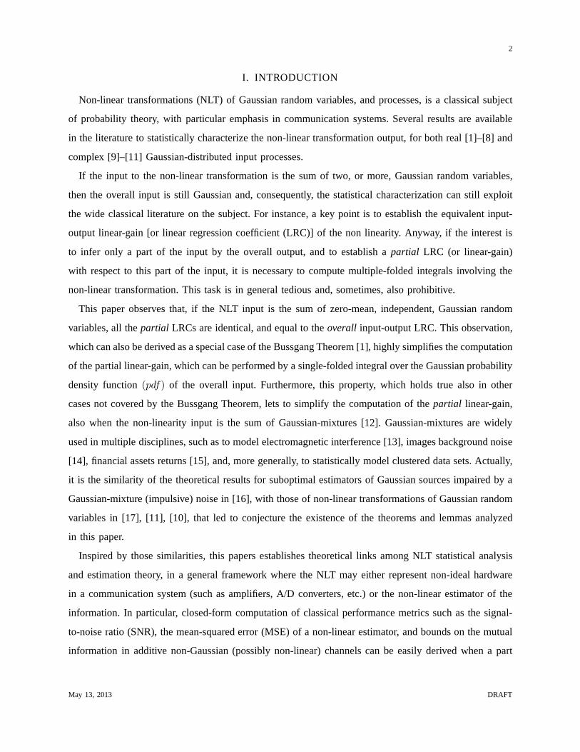
X
N
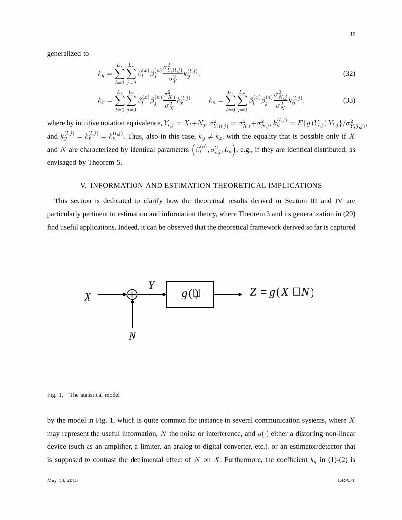
Y( )Z g X N= +( )g ⋅
Fig. 1. The statistical model
by the model in Fig. 1, which is quite common for instance in several communication systems, whereX
may represent the useful information,N the noise or interference, andg(·) either a distorting non-linear
device (such as an amplifier, a limiter, an analog-to-digital converter, etc.), or an estimator/detector that
is supposed to contrast the detrimental effect ofN on X. Furthermore, the coefficientky in (1)-(2) is
May 13, 2013 DRAFT
11
the same coefficient that appears in the Bussgang theorem [1], which lets to extend (1) to some special
random processes, such as the Gaussian ones. Specifically, for the class of stationary Bussgang processes
[21], [22], it holds true that
Z(t) = kyY (t) +Wy(t), (34)
where
ky =RZY (0)
RY Y (0)=
E{Z(t)Y (t+ τ)}E{Y 2(t)} ,∀t,∀τ, (35)
RZY (τ) = E{Z(t)Y (t+ τ)} is the classical cross-correlation function for stationary random processes,
andRWyY (τ) = 0, ∀τ . As detailed in Appendix B the Bussgang theorem [1] can be exploited to prove
Theorem 3. Furthermore, it can also be used to characterize the power spectral density of the output of
a non linearity with Gaussian input processes. This fact induced an extensive technical literature, with
closed form solutions for the computation of the LRCky for a wide class of NLTg(·), as detailed in
[1]–[8] for real Gaussian inputs, and in [9]–[11] for complex Gaussian inputs. The Bussgang Theorem
can also be used to asses the performance of such non-linear communication systems, such as the bit-
error-rate (BER), the signal-to-noise power ratio(SNR), the maximal mutual information (capacity), and
the mean square estimation error(MSE), whose link has attracted considerable research efforts inthe last
decade (see [23], [24] and references therein). Thus, taking in mind the broad framework encompassed
by Fig. 1, the following subsections will clarify how some ofthe theorems derived in this paper impact
on the computations of the SNR, the capacity, and the MSE, andwill provide also insights on their
interplay in non-Gaussian and non-linear scenarios.
A. SNR considerations
In order to define a meaningful SNR, it is useful to separate the non-linear device output as the sum of
the useful information with an uncorrelated distortion, asin (8). For simplicity, we assume in the following
that all the random variables are zero-mean, i.e.,PX = σX2. Thus, the SNR at the non-linearity output,
is expressed by
SNRx = k2xE{X2}E{W 2
x}=
k2xσ2X
E{Z2} − k2xσ2X
=
(EY {g2(Y )}
k2xσ2X
− 1
)−1
, (36)
where the second equality is granted by the orthogonality betweenX andWx.
In the general case, in order to obtain a closed form expression for (36), it would be necessary to
solve the double folded integral in (9), for the computationof kx. However, ifX andN are zero-mean,
May 13, 2013 DRAFT
12
independent, and Gaussian, by Theorem 3 the computation canbe simplified by exploiting thatkx = ky
and, consequently, the computation of the SNR would requestto solve only single-folded integrals, e.g.,
(2) andEY {g2(Y )}. Note that, in this case alsoY = X + N would be Gaussian and, consequently,
the computations ofky andEY {g2(Y )} can benefit of the results available in the literature [1], [2], [4],
[6]–[8], [10], [11], [17]. 3
Actually, it could be argued that the SNR may be also defined byexploiting (1) rather than (8). Indeed,
by rewriting (1) as
Z = g(X +N) = kyX + kyN +Wy, (37)
it is possible to define another SNR, as expressed by
SNRy =k2yE{X2}
k2yE{N2}+ E{W 2y }
=k2yσ
2X
EY {g2(Y )} − k2yσ2X
=
(
EY {g2(Y )}k2yσ
2X
− 1
)−1
. (38)
Theorem 3 states that the two SNRs in (38) and (36) are identical if X and N are zero-mean,
independent, and Gaussian. WhenN (and/orX) is non-Gaussian, it is possible to approximate itspdf
with infinite accuracy [26] by the Gaussian-mixture (21) in Section IV, which represents a wide class
of zero-mean noises with symmetricalpdfs. In this case,kx 6= ky and (36) should be used instead of
(38). However, although (38) cannot be used to compute the SNR, Theorem 3 turns out to be useful to
computekx, by exploiting
kx =
L∑
l=0
βlk(l)x , k(l)x = k(l)y =
EYl{g(Yl)Yl}σ2Y,l
, (39)
which again involves only the computations of single-folded integrals. Note that, all the integralsEYl{g(Yl)Yl}
in (39) share the same closed-form analytical solution for the Gaussianvirtual inputsYl.
3An alternative way to simplify the computation of the lineargain kx by a single-folded integral could exploit hybrid non-
linear moments analysis of Gaussian inputs [25] [26], whereit is proven thatE{Xg(Y )} = E{X[a0 + a1(Y −E{Y })]}, with
a0 = E{g(Y )} anda1 = E{dg(Y )/dY }. WhenY = X +N , with zero-meanX andN , it leads toEXN{xg(X +N)} =
σ2
XEY {dg(Y )/dY }. This fact highlights thatky = kx = EY {dg(Y )/dY }, i.e., for Gaussian inputs the statistical linear gain
ky is equivalent to the average of the first-order term of the MacLaurin expansion of the non linearity. Similarly, ifY (N ) is a
Gaussian-Mixture, it is possible to exploitE{Xg(Y )} =∑
βlE{Xg(Yl)} andEXYl{Xg(Yl)} = σ2
XEYl{dg(Y )/dY }.
May 13, 2013 DRAFT
13
B. Estimation theory and MSE considerations
The definition of the error at the non-linearity output may depend on the non-linearity purpose. If the
NLT g(·) represents an estimator ofX given the observationY = X +N , as expressed by
X = g(X +N) = kxX +Wx, (40)
the estimation error is defined as
e = X −X = (kx − 1)X +Wx. (41)
Exploiting the uncorrelation betweenX andN , which induces
E{W 2x} = EY {g2(Y )} − k2xE{X2}, (42)
the MSE at the non-linearity output can be expressed by
MSE= E{e2}= (kx − 1)2E{X2}+ E{W 2x}
= EY {g2(Y )}+ (1− 2kx)E{X2}. (43)
However, looking at (40) from another point of view, it is also possible to considerg(·) as a distorting
device that scales bykx the useful informationX, i.e, (43) represents the MSE of a (conditionally) biased
estimator. In this view, it is possible to define an unbiased estimator Xu = X/kx and the associated
unbiased estimation error as
eu = X/kx −X = Wx/kx, (44)
whose mean square-value is expressed by
MSEu= E{e2u} = E{W 2x}/k2x
= EY {g2(Y )}/k2x − E{X2}. (45)
It is straightforward to verify that, for a given information powerE{X2}, the non-linearities that maximize
the two MSE are different, as expressed by
gmmse(·) = argming(·)
[MSE] = argming(·)
[log(MSE)]
= argming(·)
[E{g2(Y )}/kx
],
(46)
and
gu-mmse(·) = argming(·)
[MSEu] = argming(·)
[E{g2(Y )}/k2x
]. (47)
May 13, 2013 DRAFT
14
The first criterion corresponds to the classical Bayesian minimum MSE (MMSE) estimator, that is
gmmse(Y ) = EX|Y {X}. By means of (36) and (47), the second criterion, which is theunbiased-MMSE
(U-MMSE) estimator, is equivalent to the maximum-SNR (MSNR) criterion. Note thatkx depends on
g(·) by (9) and consequently, in general
gu-mmse(·) 6=gmmse(·)k(mmse)x
. (48)
Indeed, the right-hand term in (48) is a (conditionally) unbiased estimator, but not the (U-MMSE) optimal
one, because it has been obtained by first optimizing the MSE,and by successively compensating the
biasing gainkx, while gu-mmse(Y ) should be obtained the other way around, as expressed by (44)and (47).
The two criteria tend to be quite similar when the functionalderivative δkx(g(·))δg(·) ≈ 0 in the neighborhood
of the optimal solutiongmmse(·).Actually, the MMSE and the MSNR criteria are equivalent froman information theoretic point of view
only wheng(·) is linear, as detailed in [23], in which casegu-mmse(·) is equivalent to right-hand side of
(48). For instance, this happens whenX andN are both zero-mean, independent, and Gaussian as in
Theorem 3, in which case it is well known that [18]
Xmmse= gmmse(Y ) =σ2X
σ2X + σ2
N
Y =σ2X
σ2X + σ2
N
(X +N) (49)
is just a scaled version of the U-MMSE
Xu-mmse= gu-mmse(Y ) = Y = X +N. (50)
By noting that the SNR is not influenced by a scaling coefficient, because it affects both the useful
information and the noise, it is confirmed that for linearg(·) the MMSE optimal solution is also MSNR
optimal [23].
Conversely, whenN is not Gaussian distributed, itspdf may be (or approximated by) a Gaussian-
mixture as in (21). In this case, analogously to the consideration for the SNR computation, Theorem 3
turns out to be useful to computekx, and thus the MSE in (43), and (45), by the single-folded integrals
involved in (31), rather than by the double-folded integrals in (26). The reader interested in this point,
may find a deeper insights and a practical application in [27], where these considerations have been
fully exploited to characterize the performance of MMSE andMSNR estimators for a Gaussian source
impaired by impulsive Middleton’s Class-A noise.
C. Capacity considerations
Equations (8) or (37) can also be exploited to compute the mutual information of the non-linear
information channelX → Z = g(X + N) summarized by Fig. 1. Actually, the exact computation of
May 13, 2013 DRAFT
15
the mutual information is in general prohibitive due to the complicated expression for thepdf of the
two disturbance componentsWx andkyN +Wy, in (8) and (37), respectively. Anyway, it is possible to
exploit the theoretical results derived so far, to establish some useful bounds on the mutual information
in a couple of scenarios, as detailed in the following.
1) Non-linear channels with non-Gaussian noise:
When the noiseN is not Gaussian, it is difficult to compute in closed form the mutual information
I(X → Y ) even in the absence of the non-linearityg(·), and only bounds are in general available
[28]. Actually, when the noiseN is the Gaussian-mixture summarized by (21), it does not either exist
a closed form expression for the differential entropyh(N), which can only be bounded as suggested
in [29]. However, whenX is Gaussian, the results in this paper can be exploited to compute simple
lower-bounds for the mutual informationI(X,Z) at the output of any non linearityZ = g(Y ), which
may model for instance A/D converters, amplifiers, and so forth. These lower bounds are provided by the
AWGN capacity of (8) and (37), when the disturbance is modeled as (the maximum-entropy [30]) zero-
mean Gaussian noise with varianceE{Z2}− k2xσ
2X andE
{Z2}− k2yσ
2X , respectively. Thus, exploiting
(8) and (36), it is possible to conclude that
I(X,Z) ≥ C(snrx)g(·) =
1
2log(1 + SNRx), (51)
while, by exploiting (37) and (38), it would be possible to conclude that
I(X,Z) ≥ C(snry)g(·) =
1
2log(1 + SNRy). (52)
By Theorem 3, the two lower-bounds are equivalent ifX andN are zero-mean independent Gaussians.
Otherwise, the correct SNR is (36) and the correct lower bound is (51). For instance, in the simulation
examples either whenN is Laplace distributed and independent ofX (see Fig. 2(c)), or when it is
Gaussian distributed and positively correlated withX (see Fig. 2(d)),kx > ky and consequently by (36)
and (38),C(snrx)g(·) > C
(snry)g(·) . As detailed in the previous subsections, the computationsof such lower bounds
are simplified by the results in this paper whenX is zero-mean Gaussian, andN is either zero-mean
Gaussian or a Gaussian mixture.
2) Linear channels with non-Gaussian noise:
It is also possible to derive a bound for the mutual information of the non-Gaussian additive channel
Y = X+N , in the absence or before the NLTg(·), by exploiting the interplay between MSE and mutual
information. Indeed, for non-Gaussian additive channels,exploiting the corollary of Theorem 8.6.6 in
May 13, 2013 DRAFT
16
[31], it is possible to readily derive that
I(X,Y ) ≥ h(X)− 1
2log (2πe MSE) . (53)
which holds true for the MSE of any estimatorX = g(Y ). Thus, for a Gaussian sourceX, (53) simply
becomes
I(X,Y ) ≥ C (mse)g(·) =
1
2log
(σ2X
MSE
)
, (54)
where, the lower boundC (mse)g(·) can be computed by plugging (43) in (54). Taking in mind that an estimator
is generally non-linear, it is possible to exploit the information processing inequality [31], to establish
another lower bound by means of (51)
I(X,Y ) ≥ I(X, X(Y )) ≥ C(snrx)gmmse(·), (55)
by properly computing the linear gainkx and output powerE{X(y)2} associated to the estimatorX(Y ).
It is natural to ask which of the two bounds in (54) and (55) is the tightest, and should be used in
practice. To this end, lets note that by (36) and (43) MSE and SNRx are linked by
SNRx =k2xσ
2X
E{W 2x}
=k2xσ
2X
MSE− (1− kx)2 σ2
X
, (56)
which lets to establish the following general Theorem
Theorem 6: For any additive noise channelY = X+N , and any estimatorX(Y ), the capacity lower
bound based on theSNR is always tighter, (or at least equivalent), than the capacity lower bound based
on theMSE, as summarized by
C(snrx)g(·) ≥ C
(mse)g(·) . (57)
Proof: See Appendix C.
The two lower bounds are a valuable alternative to the pessimistic lower bound that models the noise as
completely Gaussian, which is expressed by
I(X,Y ) ≥ CAWGN =1
2log(1 + SNR), (58)
where the total SNR is defined as SNR= σ2x
σ2n
. For any estimator such that MSE≤ σ2n
SNRSNR+1 , by means of
(54) and (58),C(mse)g(·) ≥ CAWGN. Actually, any useful estimator should significantly reduce the estimation
error power with respect to the original noise power [e.g., the estimation error power withg(y) = y],
as expressed by MSE≪ σ2n: this fact consequently induces thatC
(mse)g(·) > CAWGN is verified for any
practical estimator and SNR, as it will be confirmed in the simulations section. Note that, the lower
May 13, 2013 DRAFT
17
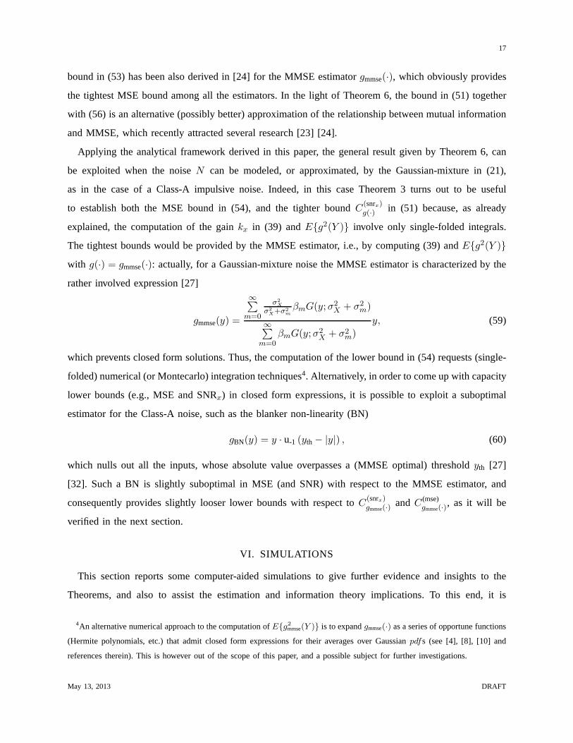
bound in (53) has been also derived in [24] for the MMSE estimator gmmse(·), which obviously provides
the tightest MSE bound among all the estimators. In the lightof Theorem 6, the bound in (51) together
with (56) is an alternative (possibly better) approximation of the relationship between mutual information
and MMSE, which recently attracted several research [23] [24].
Applying the analytical framework derived in this paper, the general result given by Theorem 6, can
be exploited when the noiseN can be modeled, or approximated, by the Gaussian-mixture in(21),
as in the case of a Class-A impulsive noise. Indeed, in this case Theorem 3 turns out to be useful
to establish both the MSE bound in (54), and the tighter boundC(snrx)g(·) in (51) because, as already
explained, the computation of the gainkx in (39) andE{g2(Y )} involve only single-folded integrals.
The tightest bounds would be provided by the MMSE estimator,i.e., by computing (39) andE{g2(Y )}with g(·) = gmmse(·): actually, for a Gaussian-mixture noise the MMSE estimatoris characterized by the
rather involved expression [27]
gmmse(y) =
∞∑
m=0
σ2X
σ2X+σ2
m
βmG(y;σ2X + σ2
m)
∞∑
m=0βmG(y;σ2
X + σ2m)
y, (59)
which prevents closed form solutions. Thus, the computation of the lower bound in (54) requests (single-
folded) numerical (or Montecarlo) integration techniques4. Alternatively, in order to come up with capacity
lower bounds (e.g., MSE and SNRx) in closed form expressions, it is possible to exploit a suboptimal
estimator for the Class-A noise, such as the blanker non-linearity (BN)
gBN(y) = y · u-1 (yth − |y|) , (60)
which nulls out all the inputs, whose absolute value overpasses a (MMSE optimal) thresholdyth [27]
[32]. Such a BN is slightly suboptimal in MSE (and SNR) with respect to the MMSE estimator, and
consequently provides slightly looser lower bounds with respect toC(snrx)gmmse(·) andC (mse)
gmmse(·), as it will be
verified in the next section.
VI. SIMULATIONS
This section reports some computer-aided simulations to give further evidence and insights to the
Theorems, and also to assist the estimation and informationtheory implications. To this end, it is
4An alternative numerical approach to the computation ofE{g2mmse(Y )} is to expandgmmse(·) as a series of opportune functions
(Hermite polynomials, etc.) that admit closed form expressions for their averages over Gaussianpdfs (see [4], [8], [10] and
references therein). This is however out of the scope of thispaper, and a possible subject for further investigations.
May 13, 2013 DRAFT
18
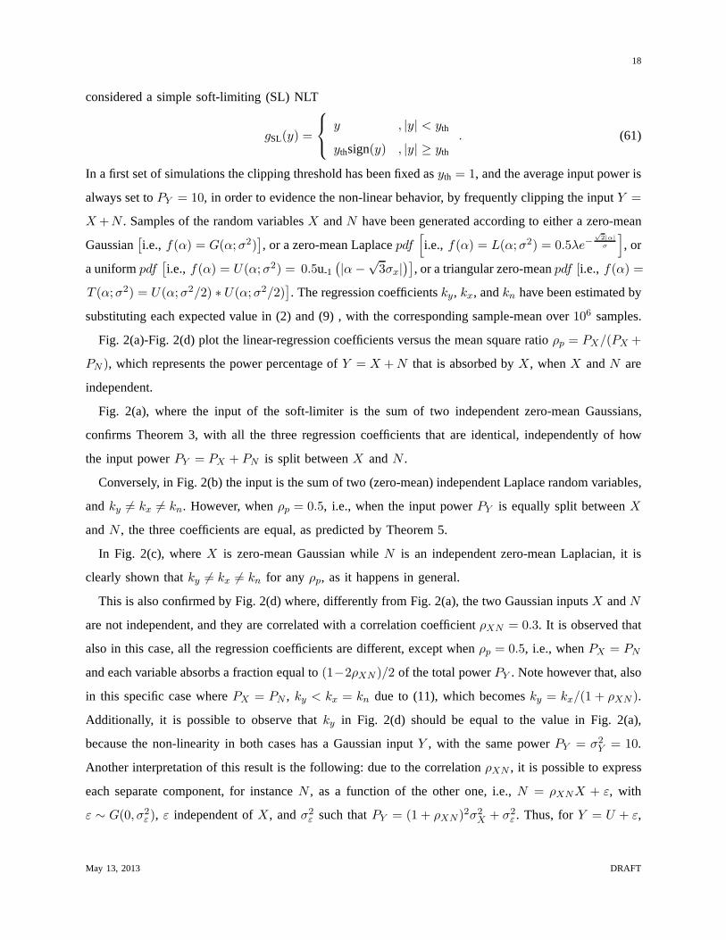
considered a simple soft-limiting (SL) NLT
gSL(y) =
y , |y| < yth
ythsign(y) , |y| ≥ yth
. (61)
In a first set of simulations the clipping threshold has been fixed asyth = 1, and the average input power is
always set toPY = 10, in order to evidence the non-linear behavior, by frequently clipping the inputY =
X+N . Samples of the random variablesX andN have been generated according to either a zero-mean
Gaussian[i.e., f(α) = G(α;σ2)
], or a zero-mean Laplacepdf
[
i.e., f(α) = L(α;σ2) = 0.5λe−√
2|α|σ
]
, or
a uniformpdf[i.e., f(α) = U(α;σ2) = 0.5u-1
(|α−
√3σx|
)], or a triangular zero-meanpdf [i.e., f(α) =
T (α;σ2) = U(α;σ2/2) ∗ U(α;σ2/2)]. The regression coefficientsky, kx, andkn have been estimated by
substituting each expected value in (2) and (9) , with the corresponding sample-mean over106 samples.
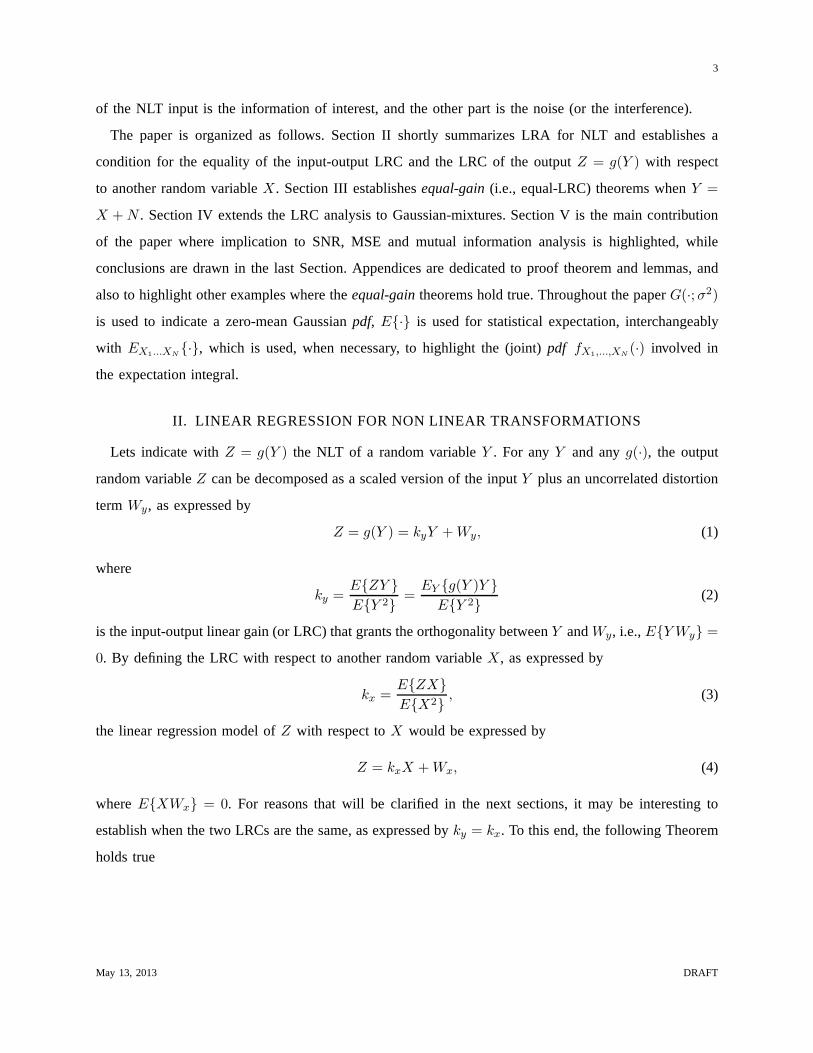
Fig. 2(a)-Fig. 2(d) plot the linear-regression coefficients versus the mean square ratioρp = PX/(PX +
PN ), which represents the power percentage ofY = X +N that is absorbed byX, whenX andN are
independent.
Fig. 2(a), where the input of the soft-limiter is the sum of two independent zero-mean Gaussians,
confirms Theorem 3, with all the three regression coefficients that are identical, independently of how
the input powerPY = PX + PN is split betweenX andN .
Conversely, in Fig. 2(b) the input is the sum of two (zero-mean) independent Laplace random variables,
andky 6= kx 6= kn. However, whenρp = 0.5, i.e., when the input powerPY is equally split betweenX
andN , the three coefficients are equal, as predicted by Theorem 5.
In Fig. 2(c), whereX is zero-mean Gaussian whileN is an independent zero-mean Laplacian, it is
clearly shown thatky 6= kx 6= kn for any ρp, as it happens in general.
This is also confirmed by Fig. 2(d) where, differently from Fig. 2(a), the two Gaussian inputsX andN
are not independent, and they are correlated with a correlation coefficientρXN = 0.3. It is observed that
also in this case, all the regression coefficients are different, except whenρp = 0.5, i.e., whenPX = PN
and each variable absorbs a fraction equal to(1−2ρXN )/2 of the total powerPY . Note however that, also
in this specific case wherePX = PN , ky < kx = kn due to (11), which becomesky = kx/(1 + ρXN ).
Additionally, it is possible to observe thatky in Fig. 2(d) should be equal to the value in Fig. 2(a),
because the non-linearity in both cases has a Gaussian inputY , with the same powerPY = σ2Y = 10.
Another interpretation of this result is the following: dueto the correlationρXN , it is possible to express
each separate component, for instanceN , as a function of the other one, i.e.,N = ρXNX + ε, with
ε ∼ G(0, σ2ε ), ε independent ofX, andσ2
ε such thatPY = (1 + ρXN )2σ2X + σ2
ε . Thus, forY = U + ε,
May 13, 2013 DRAFT

19
0 0.1 0.2 0.3 0.4 0.5 0.6 0.7 0.8 0.9 10
0.05
0.1
0.15
0.2
0.25
0.3
0.35
0.4
0.45
0.5
ρp
Line
ar G
ains
ky
kx
kn
(a) X ∼ G(x;PX), N ∼ G(n;PN)
0 0.1 0.2 0.3 0.4 0.5 0.6 0.7 0.8 0.9 1
0.16
0.18
0.2
0.22
0.24
0.26
ρp
Line
ar G
ains
ky
kx
kn
(b) X ∼ L(x;PX), N ∼ L(n;PN )
0 0.1 0.2 0.3 0.4 0.5 0.6 0.7 0.8 0.9 1
0.16
0.18
0.2
0.22
0.24
0.26
0.28
ρp
Line
ar G
ains
ky
kx
kn
(c) X ∼ G(x;PX), N ∼ L(n;PN)
0 0.1 0.2 0.3 0.4 0.5 0.6 0.7 0.8 0.9 10.2
0.3
0.4
0.5
0.6
0.7
0.8
0.9
1
ρp
Line
ar G
ains
ky
kx
kn
(d) X ∼ G(x;PX), N ∼ G(n;PN ), ρXN = 0.3
Fig. 2. Linear regression coefficients versus the input power ratio, whenPY = 10 and the inputs are a) independent and
Gaussians pdfs; b) independent and Laplace pdfs; c) independent Gaussian and Laplace pdfs; d) correlated Gaussians pdfs.
U = (1 + ρXN )X the hypotheses of Theorem 3 are satisfied and consequentlyky = ku = kε, where by
straightforward substitutionsku = E{ZU}/PU = kx/(1 + ρXN ).
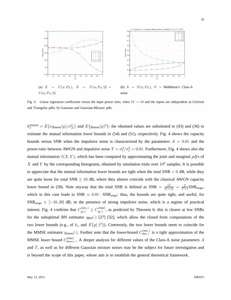
In Fig. 3(b) X ∼ U(x;σ2X) is a zero-mean uniform random variable andN ∼ T (n;σ2
N ) has an
independent zero-mean triangularpdf: it can be observed that in generalky 6= kx 6= kn unless when
PN = 2PX = 2PY /3 (ρp = 1/3), i.e., whenfN(n) = fX(n) ∗ fX(n). This fact confirms Example
1 in Appendix A, where, generalizing Theorem 5, it has been highlighted that in this caseY can be
interpreted asY = X + (N1 + N2), e.g., as the sum of three (uniform) i.i.d. random variables, and
ky = kx = kn1= kn2
.
A final set of results is dedicated to derive capacity bounds for a Gaussian sourceX impaired by an
impulsive noiseN , modeled as a Gaussian mixture, according to the Middleton’s Class-A noise model.
The analytical expression in (59) has been used to compute bya Montecarlo semi-analytical approach
May 13, 2013 DRAFT
20
0 0.1 0.2 0.3 0.4 0.5 0.6 0.7 0.8 0.9 10.18
0.2
0.22
0.24
0.26
0.28
0.3
ρp
Line
ar G
ains
ky
kx
kn
(a) X ∼ U(x;PX), N ∼ U(n;PN/2) ∗
U(n;PN/2)
0 0.1 0.2 0.3 0.4 0.5 0.6 0.7 0.8 0.9 10
0.1
0.2
0.3
0.4
0.5
0.6
0.7
0.8
0.9
ρp
Line
ar G
ains
X = Gaussian , N = Gaussian−Mixture (Class−A model) [ A = 0.1 ; T = 0.01 ]
k
y
kx
kn
(b) X ∼ N(x;PX), N ∼ Middleton’s Class-A
noise
Fig. 3. Linear regression coefficients versus the input power ratio, whenPY = 10 and the inputs are independent a) Uniform
and Triangular pdfs; b) Gaussian and Gaussian-Mixture pdfs
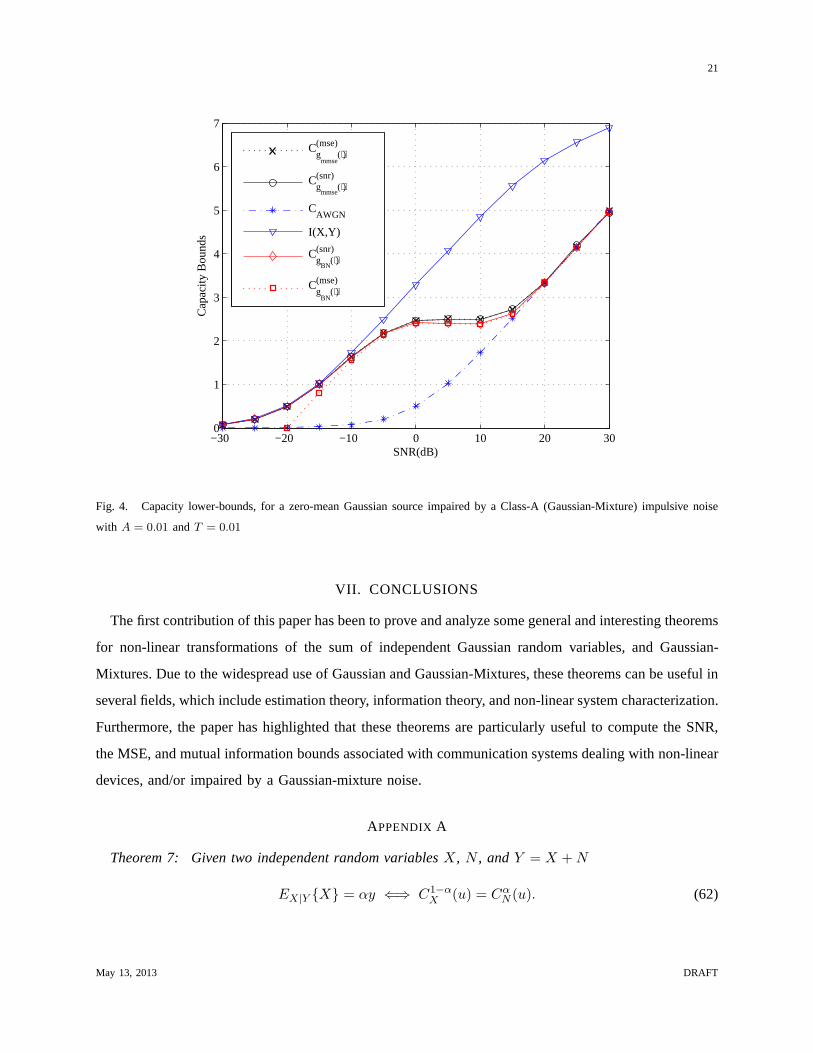
k(mmse)x = E{xgmmse(y)/σ
2X} andE{gmmse(y)
2}: the obtained values are substituted in (43) and (36) to
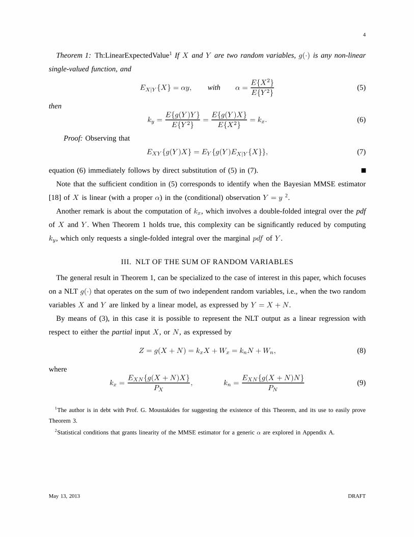
estimate the mutual information lower bounds in (54) and (51), respectively. Fig. 4 shows the capacity
bounds versus SNR when the impulsive noise is characterizedby the parametersA = 0.01 and the
power-ratio between AWGN and impulsive noiseT = σ2t /σ
2I = 0.01. Furthermore, Fig. 4 shows also the
mutual informationI(X,Y ), which has been computed by approximating the joint and marginal pdfs of
X andY by the corresponding histograms, obtained by simulation trials over108 samples. It is possible
to appreciate that the mutual information lower bounds are tight when the total SNR< 0 dB, while they
are quite loose for total SNR≥ 10 dB, where they almost coincide with the classical AWGN capacity
lower bound in (58). Note anyway that the total SNR is defined as SNR = σ2x
σ2t+σ2
I
= TT+1SNRawgn,
which in this case leads to SNR≃ 0.01 · SNRawgn: thus, the bounds are quite tight, and useful, for
SNRawgn ∈ [−10, 20] dB, in the presence of strong impulsive noise, which is a regime of practical
interest. Fig. 4 confirms thatC(snrx)g(·) ≥ C
(mse)g(·) , as predicted by Theorem 6: this is clearer at low SNRs
for the suboptimal BN estimatorgBN(·) [27] [32], which allow the closed form computations of the
two lower bounds (e.g., ofkx andE{g(·)2}). Conversely, the two lower bounds seem to coincide for
the MMSE estimatorgmmse(·). Further note that the lower-boundC(snrx)gBN(·) is a tight approximation of the
MMSE lower boundC(mse)gmmse(·) . A deeper analysis for different values of the Class-A noiseparametersA
andT , as well as for different Gaussian mixture noises may be the subject for future investigation and
is beyond the scope of this paper, whose aim is to establish the general theoretical framework.
May 13, 2013 DRAFT
21
−30 −20 −10 0 10 20 300
1
2
3
4
5
6
7
SNR(dB)
Cap
acity
Bou
nds
Cg
mmse(⋅)
(mse)
Cg
mmse(⋅)
(snr)
CAWGN
I(X,Y)
Cg
BN(⋅)
(snr)
Cg
BN(⋅)
(mse)
Fig. 4. Capacity lower-bounds, for a zero-mean Gaussian source impaired by a Class-A (Gaussian-Mixture) impulsive noise
with A = 0.01 andT = 0.01
VII. CONCLUSIONS
The first contribution of this paper has been to prove and analyze some general and interesting theorems
for non-linear transformations of the sum of independent Gaussian random variables, and Gaussian-
Mixtures. Due to the widespread use of Gaussian and Gaussian-Mixtures, these theorems can be useful in
several fields, which include estimation theory, information theory, and non-linear system characterization.
Furthermore, the paper has highlighted that these theoremsare particularly useful to compute the SNR,
the MSE, and mutual information bounds associated with communication systems dealing with non-linear
devices, and/or impaired by a Gaussian-mixture noise.
APPENDIX A
Theorem 7: Given two independent random variablesX, N , andY = X +N
EX|Y {X} = αy ⇐⇒ C1−αX (u) = Cα
N (u). (62)
May 13, 2013 DRAFT
22
Proof: Observing that
EX|Y {X} =
∫ +∞
−∞xfX|Y (x; y)dx =
1
fY (y)
∫ +∞
−∞xfXY (x, y)dx, (63)
clearly l.h.s. of (63) holds true if and only if∫ +∞
−∞xfXY (x, y)dx = αyfY (y). (64)
If Y = X +N , with X independent ofN , it is well known [19] thatfXY (x, y) = fX(x)fY |X(y;x) =
fX(x)fN (y−x) andfY (y) = fX(y)∗fN (y), where∗ stands for the convolution integral operator. Thus,
(64) becomes
p(y) ∗ fN(y) = αy · [fX(y) ∗ fN(y)] , (65)
wherep(x) = xfX(x). By applying the inverse Fourier transform, (65) becomes
P (u)CN (u) =α
j2π
d
du[CX(u)CN (u)], (66)
whereP (u) = 1j2π
ddu [CX(u)] = 1
j2πC′
X(u), and consequently
C′
X(u)CN (u) = α[
C′
X(u)CN (u) + CX(u)C′
N (u)]
. (67)
The last equality is a differential equation, with separable variables, as expressed by
(1− α)C
′
X(u)
CX(u)= α
C′
N (u)
CN (u), (68)
which can be solved by direct integration, leading to
(1− α)log (CX(u)) = αlog(CN (u)) + Co, (69)
whereCo = 0 is imposed by the boundary conditionsCX(0) = CN (0) = 1. Equation (69) is equivalent
to
C1−αX (u) = Cα
N (u), (70)
which concludes the proof.
It is possible to observe that, for a givenfX(x) [or a givenfN(n)], (70) and (62) do not always admit
a solutionfN (n) [or fX(x)]. For a fixedpdf fX(x), the existence of a solution is equivalent to
fN (n) = F−1{CρX(u)}, (71)
i.e., to the existence of the inverse Fourier transform ofCρX(u), whereρ = 1−α
α = PY −PX
PX. To this end, it
can be observed that∀ρ > 0 the functionCρX(u) preserves the conjugate symmetry ofCX(u) = C∗
X(−u)
and the unitary area of thepdf by CX(0) = 1. Moreover, if ρ ∈ [0, 1] and if∫ +∞−∞ |CX(u)|du < +∞,
May 13, 2013 DRAFT
23
then also∫ +∞−∞ |Cρ
X(u)|du < +∞, which is a sufficient condition for the existence of the inverse Fourier
transform. Although it is beyond the scope of the paper to establish (if possible) all the possible conditions
where (70) or (71) admit feasible solutions, it is highlighted thatρ = PN
PXwhenX andN are independent,
and consequentlyρ ∈ [0, 1] whenPX ≥ PN . Furthermore, some examples are listed in the following to
clarify the subject and identifying some specific cases of interest.
Example 1: If α = p/q < 1 with p, q ∈ N, i.e.,α ∈ Q, then (70) is equivalent to
Cq−pX (u) = Cp
N (u). (72)
This means that for a fixedfX(x), and a fixedα = p/q < 1, Theorem 7 holds true if the random variable
N is characterized by apdf fN (n) that satisfies
fN (n) ∗ · · · ∗︸ ︷︷ ︸
q−p−1
fN(n) = fX(n) ∗ · · · ∗︸ ︷︷ ︸
p
fX(n). (73)
Note that (73) is a (multiple) auto-deconvolution problem in fN (n), which is well known to be ill-
posed for several functionsh(n) = fX(n) ∗ · · · ∗︸ ︷︷ ︸
p
fX(n), even in the simple caseq − p = 2 where
fN (n) ∗ fN (n) = h(n).
The problem admits a solution whenα = 2/3 (ρ = 1/2), where it boils down tofN (n) = fX(n)∗fX (n).
This means thatN can be thought as the sum of two other (independent) random variablesN = N1+N2,
each one with the same distribution ofX. This is actually equivalent to a generalization of Theorem5 to
the sum of three i.i.d. random variables. The generalization to the sum ofQ+ 1 i.i.d. random variables
is obtained forα = Q/(Q+ 1) (ρ = 1/Q).
Example 2: If X is Gaussian, with meanmX and varianceσ2X , then (70) (apparently) admits always
a solution for anyα ∈ [0, 1], and would lead us to (erroneously) conclude that alsofN (n) should be
non-zero mean Gaussian. Indeed, the characteristic function of a Gaussianpdf is a Gaussian function,
and any (positive) exponential of a Gaussian function is still a Gaussian function. Thus, recalling that
CX(u) = e−2(πσXu)2+j2πmXu, we would conclude that
fN (n) = F−1{CρX(u)} = F−1{e−2(π
√ρσXu)
2+j2πρmXu} = G(n− ρmX ; ρσ2
X), (74)
which holds true whenρ > 0, i.e., whenα ∈ [0, 1] andPY > PX . Actually, it should be observed that
right-hand side of (74) implicitly contains the constraints σ2N = ρσ2
X , mN = ρmX that, by the definition
of ρ, can be jointly satisfiediff mX = mN = 0, and∀σX ,∀σN . Thus, the equal gain condition holds
true for Gaussian inputs, only if they are zero-mean, as expressed by Theorem 3.
May 13, 2013 DRAFT
24
Example 3:Whenα = 1/2, i.e.,ρ = 1, equation (62) boils down to the trivial caseCX(u) = CN (u),
i.e., the sufficient condition forky = kx = kn is satisfied if the independent random variablesX andN
are identically distributed (and zero-mean) withfX(·) = fN (·). This is an alternative proof for Theorem
5.
APPENDIX B
An alternative proof of Theorem 3 for Gaussians r.v. can exploit the Bussgang Theorem for jointly-
Gaussian random processesx(t) andy(t), which states that [1], [17], [19]
E{x(t)g[y(t + τ)]} =E{y(t)g[y(t + τ)]}
σ2Y
E{x(t)y(t + τ)} ,∀τ. (75)
SettingX = x(t), Y = y(t), andτ = 0, then (75) easily leads to
kx = kyE{XY }
σ2X
, (76)
which reduces tokx = ky for Y = X+N , whenX andN are zero-mean and independent (and Gaussian
to let Y be Gaussian).
Some Lemmas of Theorem 3 follow.
Lemma 1: IfX andN are zero-mean Gaussian and independent,Y = αxX+αnN , with αx, αn ∈ R,
thenE{ZY }
σ2Y
=1
αx
E{ZX}σ2X
=1
αn
E{ZN}σ2N
.
Proof: By Theorem 3 withX = αxX andN = αnN .
Lemma 2: If Y =J∑
j=1αjXj, αj ∈ R, Xj and N are independent zero-mean Gaussian random
variables, thenE{ZY }
σ2Y
=1
αi
E{ZXi}σ2Xi
,∀i.
Proof: By Theorem 1 and Lemma 1 withX = αiXi andN =∑
(j 6=i)
αjXj .
APPENDIX C
PROOF OFTHEOREM 6
Proving thatC(snrx)lb > C
(mse)lb corresponds to prove that1 + SNRx > σ2
X
MSE. Thus, when|kx| ≥ 1 it is
straightforward to verify that
1 +k2xσ
2X
PWx
= 1 +k2xσ
2X
MSE− (1− kx)2 σ2
X
≥ 1 +k2xσ
2X
MSE>
σ2X
MSE. (77)
May 13, 2013 DRAFT
25
More generally the inequality1 + SNRx > σ2X
MSE holds true when
PWx+ k2xσ
2X
PWx
≥ σ2X
PWx+ (1− kx)
2 σ2X
, (78)
that is when
P 2Wx
+ 2PWxkx (1− kx)σ
2X + (1− kx)
2 k2xσ2X ≥ 0. (79)
Clearly, (79) holds true when|kx| ≤ 1, which together with (77) lets to conclude that the inequality
holds true for∀kx ∈ R, concluding the proof.
REFERENCES
[1] J. J. Bussgang, “Crosscorrelation functions of amplitude-distorted gaussian signals,”M.I.T. RLE Technical Report, no.
216, pp. 1 –14, march 1952. [Online]. Available: http://hdl.handle.net/1721.1/4847
[2] R. Baum, “The correlation function of smoothly limited guassian noise,”IRE Trans. Inf. Theory, vol. IT-3, pp. 193–197,
Sep 1957.
[3] R. Price, “A useful theorem for nonlinear devices havinggaussian inputs,”IRE Trans. Inform. Theory, vol. 4, pp. 69–72,
June 1958.
[4] W. B. Davenport Jr. and W. L. Root,An Introduction to the Theory of Random Signals and Noise. Mc Graw Hill, 1958.
[5] N. Blachman, “The uncorrelated output components of a nonlinearity,” IEEE Trans. Inf. Theory, vol. 14, no. 2, pp. 250–255,
Mar 1968.
[6] J. H. Van Vleck and D. Middleton, “The spectrum of clippednoise,” Proc. IEEE, vol. 54, no. 1, pp. 2–19, 1966.
[7] R. Baum, “The correlation function of gaussian noise passed through nonlinear devices,”Proc. IEEE, vol. 15, no. 4, pp.
448–456, July 1969.
[8] B. R. Levin and A. Sokova,Fondements theoriques de la radiotechnique statistique. Editions Mir, 1973.
[9] J. Minkoff, “The role of am-to-pm conversion in memoryless nonlinear systems,”IEEE Trans. Commun., vol. 33, no. 2,
pp. 139–144, 1985.
[10] P. Banelli and S. Cacopardi, “Theoretical analysis andperformance of ofdm signals in nonlinear awgn channels,”IEEE
Trans. Commun., vol. 48, no. 3, pp. 430–441, Mar 2000.
[11] D. Dardari, V. Tralli, and A. Vaccari, “A theoretical characterization of nonlinear distortion effects in ofdm systems,” IEEE
Trans. Commun., vol. 48, no. 10, pp. 1755–1764, Oct 2000.
[12] S. V. Vaseghi,Advanced digital signal processing and noise reduction, 4th ed. Chichester, UK: John Wiley & Son’s,
2009.
[13] D. Middleton, “Statistical-physical models of urban radio-noise environments - part i: Foundations,”IEEE Trans.
Electromagn. Compat., vol. EMC-14, no. 2, pp. 38–56, May 1972.
[14] D.-S. Lee, “Effective gaussian mixture learning for video background subtraction,”IEEE Trans. Pattern Anal. Mach. Intell.,
vol. 27, no. 5, pp. 827–832, May 2005.
[15] I. Buckley, D. Saunders, and L. Seco, “Portfolio optimization when asset returns have the gaussian mixture distribution,”
Europ. Jour. of Operat. Research, vol. 185, no. 3, pp. 1434–1461, Mar 2008.
[16] S. Zhidkov, “Performance analysis and optimization ofofdm receiver with blanking nonlinearity in impulsive noise
environment,”IEEE Trans. Veh. Technol., vol. 55, no. 1, pp. 234–242, Jan 2006.
May 13, 2013 DRAFT

26
[17] H. E. Rowe, “Memoryless nonlinearities with gaussian inputs: Elementary results,”Bell Syst. Tech. J., vol. 61, no. 7, pp.
1519–1525, Sep 1982.
[18] S. M. Kay, Fundamentals of Statistical Signal Processing. Vol. 1, Estimation Theory. Prentice-Hall, 1993.
[19] A. Papoulis,Probability, Random Variables, and Stochastic Processes. McGraw-Hill, 1991.
[20] L. A. Berry, “Understanding middleton’s canonical formula for class a noise,”IEEE Trans. Electromagn. Compat., vol.
EMC-23, no. 4, pp. 337–344, Nov 1981.
[21] A. H. Nuttall, “Theory and application of the separableclass of random processes,” Ph.D. dissertation, Massachusetts
Institute of Technology, Dept. of Electrical Engineering,1958.
[22] F. Rocca, B. Godfrey, and F. Muir, “Bussgang processes,” Stanford Exploration Project, Tech. Rep. 16, Apr 1979, available
at http://sepwww.stanford.edu.
[23] D. Guo, S. Shamai (Shitz), and S. Verdu, “Mutual information and minimum mean-square error in gaussian channels,”
IEEE Trans. Inf. Theory, vol. 51, no. 4, pp. 1261–1283, Apr 2005.
[24] S. Prasad, “Certain relations between mutual information and fidelity of statistical estimation,”arXiv preprint
http://arxiv.org/abs/1010.1508v1., Oct 2010.
[25] L. Cheded, “Invariance property of gaussian signals: anew interpretation, extension and applications,”Circuits, systems,
and signal processing, vol. 16, no. 5, pp. 523–536, Sep 1997.
[26] G. Scarano, “Cumulant series expansion of hybrid nonlinear moments of complex random variables,”IEEE Trans. Signal
Process., vol. 39, no. 4, pp. 1001–1003, Apr 1991.
[27] P. Banelli, “Bayesian estimation of gaussian sources in middleton’s class-a impulsive noise,”arXiv:1111.6828v2 [cs.IT],
pp. 1 –30, November 2011. [Online]. Available: http://arxiv.org/abs/1111.6828v1
[28] S. Ihara, “On the capacity of channels with additive non-gaussian noise,”Information and Control, vol. 37, no. 1, pp.
34–39, Apr 1978.
[29] M. F. Huber, T. Bailey, H. Durrant-Whyte, and U. D. Hanebeck, “On entropy approximation for gaussian mixture random
vectors,” in IEEE Int. Conf. on Multis. Fusion and Integr. for Intell. Syst. IEEE, Aug 2008, pp. 181–188.
[30] S. N. Diggavi and T. M. Cover, “The worst additive noise under a covariance constraint,”IEEE Trans. Inf. Theory, vol. 47,
no. 7, pp. 3072–3081, Nov 2001.
[31] T. M. Cover and J. A. Thomas,Elements of Information Theory, 2nd ed. John Wiley & Sons, 2006.
[32] S. Zhidkov, “Analysis and comparison of several simpleimpulsive noise mitigation schemes for ofdm receivers,”IEEE
Trans. Commun., vol. 56, no. 1, pp. 5–9, Jan 2008.
May 13, 2013 DRAFT
Related Documents