1 Modern Compiler Implementation in Java, Second Edition ...

1

Modern Compiler Implementation in Java, Second Edition

by Andrew W. Appel and Jens Palsberg ISBN:052182060x

Cambridge University Press © 2002 (501 pages) This textbook describes all phases of a compiler, and thorough coverage of current techniques in code generation and register allocation, and the compilation of functional and object-oriented languages.

Back Cover

This textbook describes all phases of a compiler: lexical analysis, parsing, abstract syntax, semantic actions, intermediate representations, instruction selection via tree matching, dataflow analysis, graph-coloring register allocation, and runtime systems. It includes good coverage of current techniques in code generation and register allocation, as well as the compilation of functional and object-oriented languages, which is missing from most books. The most accepted and successful techniques are described concisely, rather than as an exhaustive catalog of every possible variant. Detailed descriptions of the interfaces between modules of a compiler are illustrated with actual Java classes.

The first part of the book, Fundamentals of Compilation, is suitable for a one-semester first course in compiler design. The second part, Advanced Topics, which includes the compilation of object-oriented and functional languages, garbage collection, loop optimization, SSA form, instruction scheduling, and optimization for cache-memory hierarchies, can be used for a second-semester or graduate course.

This new edition has been rewritten extensively to include more discussion of Java and object-oriented programming concepts, such as visitor patterns. A unique feature in the newly redesigned compiler project in Java for a subset of Java itself. The project includes both front-end and back-end phases, so that students can build a complete working compiler in one semester.

About the Authors

Andrew W. Appel is Professor of Computer Science at Princeton University. He has done research and published papers on compilers, functional programming languages, runtime systems and garbage collection, type systems, and computer security; he is also the author of the book Compiling with Continuations. He is a designer and founder of the Standard ML of New Jersey project. In 1998, Appel was elected a Fellow of the Association for Computing Machinery for “significant research contributions in the area of programming languages and compilers” and for his work as editor-in-chief (1993-7) of the ACM Transactions on Programming Languages and Systems, the leading journal in the field of compilers and programming languages.

Hens Palsberg is Associate Professor of Computer Science at Purdue University. His research interests are programming languages, compilers, software engineering, and information security. He has authored more than 50 technical papers in these areas and a book with Michael Schwartzbach, Object-Oriented Type Systems. In 1998, he received the National Science Foundation Faculty Early Career Development Award, and in 1999, the Purdue

2

Modern Compiler Implementation in Java, Second Edition Andrew W. Appel Princeton University Jens Palsberg Purdue University

CAMBRIDGE UNIVERSITY PRESS

PUBLISHED BY THE PRESS SYNDICATE OF THE UNIVERSITY OF CAMBRIDGE The Pitt Building, Trumpington Street, Cambridge, United Kingdom

CAMBRIDGE UNIVERSITY PRESS The Edinburgh Building, Cambridge CB2 2RU, UK 40 West 20th Street, New York, NY 10011-4211, USA 477 Williamstown Road, Port Melbourne, VIC 3207, Australia Ruiz de Alarcón 13, 28014 Madrid, Spain Dock House, The Waterfront, Cape Town 8001, South Africa

http://www.cambridge.org

Copyright © 2002 Cambridge University Press

This book is in copyright. Subject to statutory exception and to the provisions of relevant collective licensing agreements, no reproduction of any part may take place without the written permission of Cambridge University Press.

First edition published 1998 Second edition published 2002

Typefaces Times, Courier, and Optima System LATEX[AU]

A catalog record for this book is available from the British Library.

Library of Congress Cataloging in Publication data

Appel, Andrew W., 1960- Modern compiler implementation in Java / Andrew W. Appel with Jens Palsberg.- [2nd ed.] p. cm. Includes bibliographical references and index.

0-521-82060-X

1. Java (Computer program language) 2. Compilers (Computer programs) I. Palsberg, Jens. II. Title. QA76.73.J38 A65 2002 005.4′53-dc21

3

2002073453

ISBN 0 521 58274 1 Modern Compiler Implementation in ML (first edition, hardback) ISBN 0 521 82060 X Modern Compiler Implementation in Java (hardback)

This textbook describes all phases of a compiler: lexical analysis, parsing, abstract syntax, semantic actions, intermediate representations, instruction selection via tree matching, dataflow analysis, graphcoloring register allocation, and runtime systems. It includes good coverage of current techniques in code generation and register allocation, as well as the compilation of functional and object-oriented languages, which is missing from most books. The most accepted and successful techniques are described concisely, rather than as an exhaustive catalog of every possible variant. Detailed descriptions of the interfaces between modules of a compiler are illustrated with actual Java classes.

The first part of the book, Fundamentals of Compilation, is suitable for a one-semester first course in compiler design. The second part, Advanced Topics, which includes the compilation of object-oriented and functional languages, garbage collection, loop optimization, SSA form, instruction scheduling, and optimization for cache-memory hierarchies, can be used for a second-semester or graduate course.

This new edition has been rewritten extensively to include more discussion of Java and object-oriented programming concepts, such as visitor patterns. A unique feature is the newly redesigned compiler project in Java for a subset of Java itself. The project includes both front-end and back-end phases, so that students can build a complete working compiler in one semester.

Andrew W. Appel is Professor of Computer Science at Princeton University. He has done research and published papers on compilers, functional programming languages, runtime systems and garbage collection, type systems, and computer security; he is also author of the book Compiling with Continuations. He is a designer and founder of the Standard ML of New Jersey project. In 1998, Appel was elected a Fellow of the Association for Computing Machinery for "significant research contributions in the area of programming languages and compilers" and for his work as editor-in-chief (1993-97) of the ACM Transactions on Programming Languages and Systems, the leading journal in the field of compilers and programming languages.

Jens Palsberg is Associate Professor of Computer Science at Purdue University. His research interests are programming languages, compilers, software engineering, and information security. He has authored more than 50 technical papers in these areas and a book with Michael Schwartzbach, Object-oriented Type Systems. In 1998, he received the National Science Foundation Faculty Early Career Development Award, and in 1999, the Purdue University Faculty Scholar award.

4

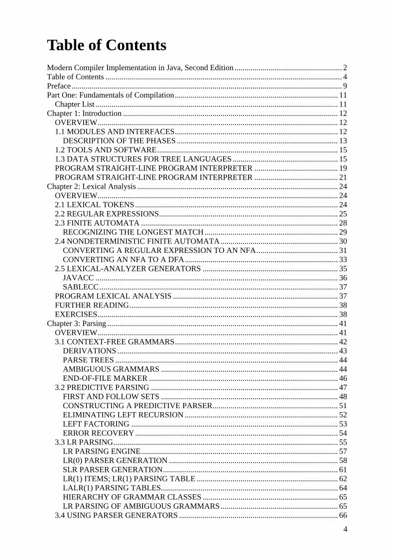
Table of Contents Modern Compiler Implementation in Java, Second Edition ...................................................... 2 Table of Contents ....................................................................................................................... 4 Preface........................................................................................................................................ 9 Part One: Fundamentals of Compilation.................................................................................. 11

Chapter List .......................................................................................................................... 11 Chapter 1: Introduction ............................................................................................................ 12

OVERVIEW......................................................................................................................... 12 1.1 MODULES AND INTERFACES.................................................................................. 12

DESCRIPTION OF THE PHASES ................................................................................. 13 1.2 TOOLS AND SOFTWARE........................................................................................... 15 1.3 DATA STRUCTURES FOR TREE LANGUAGES ..................................................... 15 PROGRAM STRAIGHT-LINE PROGRAM INTERPRETER .......................................... 19 PROGRAM STRAIGHT-LINE PROGRAM INTERPRETER .......................................... 21

Chapter 2: Lexical Analysis ..................................................................................................... 24 OVERVIEW......................................................................................................................... 24 2.1 LEXICAL TOKENS...................................................................................................... 24 2.2 REGULAR EXPRESSIONS.......................................................................................... 25 2.3 FINITE AUTOMATA ................................................................................................... 28

RECOGNIZING THE LONGEST MATCH ................................................................... 29 2.4 NONDETERMINISTIC FINITE AUTOMATA ........................................................... 30

CONVERTING A REGULAR EXPRESSION TO AN NFA......................................... 31 CONVERTING AN NFA TO A DFA............................................................................. 33

2.5 LEXICAL-ANALYZER GENERATORS .................................................................... 35 JAVACC .......................................................................................................................... 36 SABLECC........................................................................................................................ 37

PROGRAM LEXICAL ANALYSIS ................................................................................... 37 FURTHER READING......................................................................................................... 38 EXERCISES......................................................................................................................... 38

Chapter 3: Parsing .................................................................................................................... 41 OVERVIEW......................................................................................................................... 41 3.1 CONTEXT-FREE GRAMMARS.................................................................................. 42

DERIVATIONS ............................................................................................................... 43 PARSE TREES ................................................................................................................ 44 AMBIGUOUS GRAMMARS ......................................................................................... 44 END-OF-FILE MARKER ............................................................................................... 46

3.2 PREDICTIVE PARSING .............................................................................................. 47 FIRST AND FOLLOW SETS ......................................................................................... 48 CONSTRUCTING A PREDICTIVE PARSER............................................................... 51 ELIMINATING LEFT RECURSION ............................................................................. 52 LEFT FACTORING ........................................................................................................ 53 ERROR RECOVERY ...................................................................................................... 54

3.3 LR PARSING................................................................................................................. 55 LR PARSING ENGINE................................................................................................... 57 LR(0) PARSER GENERATION ..................................................................................... 58 SLR PARSER GENERATION........................................................................................ 61 LR(1) ITEMS; LR(1) PARSING TABLE ....................................................................... 62 LALR(1) PARSING TABLES......................................................................................... 64 HIERARCHY OF GRAMMAR CLASSES .................................................................... 65 LR PARSING OF AMBIGUOUS GRAMMARS........................................................... 65

3.4 USING PARSER GENERATORS ................................................................................ 66

5

JAVACC .......................................................................................................................... 66 SABLECC........................................................................................................................ 68 PRECEDENCE DIRECTIVES........................................................................................ 69 SYNTAX VERSUS SEMANTICS.................................................................................. 72

3.5 ERROR RECOVERY.................................................................................................... 73 RECOVERY USING THE ERROR SYMBOL .............................................................. 73 GLOBAL ERROR REPAIR ............................................................................................ 75

PROGRAM PARSING........................................................................................................ 77 FURTHER READING......................................................................................................... 77 EXERCISES......................................................................................................................... 77

Chapter 4: Abstract Syntax ...................................................................................................... 81 OVERVIEW......................................................................................................................... 81 4.1 SEMANTIC ACTIONS ................................................................................................. 81

RECURSIVE DESCENT................................................................................................. 81 AUTOMATICALLY GENERATED PARSERS............................................................ 82

4.2 ABSTRACT PARSE TREES ........................................................................................ 83 POSITIONS ..................................................................................................................... 85

4.3 VISITORS...................................................................................................................... 86 ABSTRACT SYNTAX FOR MiniJava ........................................................................... 91

PROGRAM ABSTRACT SYNTAX ................................................................................... 92 FURTHER READING......................................................................................................... 92 EXERCISES......................................................................................................................... 93

Chapter 5: Semantic Analysis .................................................................................................. 94 OVERVIEW......................................................................................................................... 94 5.1 SYMBOL TABLES ....................................................................................................... 94

MULTIPLE SYMBOL TABLES .................................................................................... 95 EFFICIENT IMPERATIVE SYMBOL TABLES........................................................... 96 EFFICIENT FUNCTIONAL SYMBOL TABLES.......................................................... 97 SYMBOLS....................................................................................................................... 98

5.2 TYPE-CHECKING MiniJava ...................................................................................... 100 ERROR HANDLING .................................................................................................... 102

PROGRAM TYPE-CHECKING ....................................................................................... 103 EXERCISES....................................................................................................................... 103

Chapter 6: Activation Records ............................................................................................... 105 OVERVIEW....................................................................................................................... 105

HIGHER-ORDER FUNCTIONS .................................................................................. 105 6.1 STACK FRAMES........................................................................................................ 106

THE FRAME POINTER ............................................................................................... 108 REGISTERS................................................................................................................... 108 PARAMETER PASSING.............................................................................................. 109 RETURN ADDRESSES ................................................................................................ 110 FRAME-RESIDENT VARIABLES .............................................................................. 110 STATIC LINKS ............................................................................................................. 111

6.2 FRAMES IN THE MiniJava COMPILER................................................................... 112 REPRESENTATION OF FRAME DESCRIPTIONS................................................... 114 LOCAL VARIABLES ................................................................................................... 115 TEMPORARIES AND LABELS .................................................................................. 116 MANAGING STATIC LINKS...................................................................................... 117

PROGRAM FRAMES ....................................................................................................... 117 FURTHER READING....................................................................................................... 118 EXERCISES....................................................................................................................... 118

Chapter 7: Translation to Intermediate Code ......................................................................... 121 OVERVIEW....................................................................................................................... 121

6

7.1 INTERMEDIATE REPRESENTATION TREES ....................................................... 122 7.2 TRANSLATION INTO TREES .................................................................................. 124

KINDS OF EXPRESSIONS .......................................................................................... 124 SIMPLE VARIABLES .................................................................................................. 126 ARRAY VARIABLES .................................................................................................. 127 STRUCTURED L-VALUES ......................................................................................... 128 SUBSCRIPTING AND FIELD SELECTION............................................................... 129 A SERMON ON SAFETY ............................................................................................ 130 ARITHMETIC ............................................................................................................... 130 CONDITIONALS .......................................................................................................... 131 STRINGS ....................................................................................................................... 132 RECORD AND ARRAY CREATION.......................................................................... 133 WHILE LOOPS ............................................................................................................. 134 FOR LOOPS .................................................................................................................. 135 FUNCTION CALL ........................................................................................................ 135 STATIC LINKS ............................................................................................................. 136

7.3 DECLARATIONS ....................................................................................................... 136 VARIABLE DEFINITION ............................................................................................ 136 FUNCTION DEFINITION ............................................................................................ 137 FRAGMENTS................................................................................................................ 138 CLASSES AND OBJECTS ........................................................................................... 139

PROGRAM TRANSLATION TO TREES........................................................................ 139 EXERCISES....................................................................................................................... 140

Chapter 8: Basic Blocks and Traces....................................................................................... 142 OVERVIEW....................................................................................................................... 142 8.1 CANONICAL TREES ................................................................................................. 143

TRANSFORMATIONS ON ESEQ ............................................................................... 143 GENERAL REWRITING RULES ................................................................................ 145 MOVING CALLS TO TOP LEVEL ............................................................................. 147 A LINEAR LIST OF STATEMENTS........................................................................... 147

8.2 TAMING CONDITIONAL BRANCHES ................................................................... 148 BASIC BLOCKS ........................................................................................................... 148 TRACES......................................................................................................................... 149 FINISHING UP.............................................................................................................. 150 OPTIMAL TRACES...................................................................................................... 150

FURTHER READING....................................................................................................... 151 EXERCISES....................................................................................................................... 151

Chapter 9: Instruction Selection............................................................................................. 153 OVERVIEW....................................................................................................................... 153

TREE PATTERNS......................................................................................................... 153 OPTIMAL AND OPTIMUM TILINGS........................................................................ 156

9.1 ALGORITHMS FOR INSTRUCTION SELECTION ................................................ 156 MAXIMAL MUNCH .................................................................................................... 156 DYNAMIC PROGRAMMING ..................................................................................... 158 TREE GRAMMARS...................................................................................................... 159 FAST MATCHING........................................................................................................ 161 EFFICIENCY OF TILING ALGORITHMS ................................................................. 162

9.2 CISC MACHINES ....................................................................................................... 162 9.3 INSTRUCTION SELECTION FOR THE MiniJava COMPILER.............................. 165

ABSTRACT ASSEMBLY LANGUAGE INSTRUCTIONS........................................ 165 PRODUCING ASSEMBLY INSTRUCTIONS ............................................................ 167 PROCEDURE CALLS .................................................................................................. 169 IF THERE'S NO FRAME POINTER ............................................................................ 170

7

PROGRAM INSTRUCTION SELECTION...................................................................... 170 REGISTER LISTS ......................................................................................................... 171


Chapter 10: Liveness Analysis............................................................................................... 175 OVERVIEW....................................................................................................................... 175 10.1 SOLUTION OF DATAFLOW EQUATIONS .......................................................... 176

CALCULATION OF LIVENESS ................................................................................. 177 REPRESENTATION OF SETS..................................................................................... 179 TIME COMPLEXITY ................................................................................................... 179 LEAST FIXED POINTS................................................................................................ 180 STATIC VS. DYNAMIC LIVENESS........................................................................... 181 INTERFERENCE GRAPHS.......................................................................................... 182

10.2 LIVENESS IN THE MiniJava COMPILER.............................................................. 183 GRAPHS ........................................................................................................................ 183 CONTROL-FLOW GRAPHS........................................................................................ 184 LIVENESS ANALYSIS ................................................................................................ 185

PROGRAM CONSTRUCTING FLOW GRAPHS ........................................................... 186 PROGRAM LIVENESS .................................................................................................... 186 EXERCISES....................................................................................................................... 186

Chapter 11: Register Allocation............................................................................................. 188 OVERVIEW....................................................................................................................... 188 11.1 COLORING BY SIMPLIFICATION........................................................................ 188

EXAMPLE ..................................................................................................................... 189 11.2 COALESCING........................................................................................................... 191

SPILLING ...................................................................................................................... 193 11.3 PRECOLORED NODES ........................................................................................... 194

TEMPORARY COPIES OF MACHINE REGISTERS ................................................ 194 CALLER-SAVE AND CALLEE-SAVE REGISTERS ................................................ 195 EXAMPLE WITH PRECOLORED NODES ................................................................ 195

11.4 GRAPH-COLORING IMPLEMENTATION............................................................ 198 DATA STRUCTURES .................................................................................................. 199 INVARIANTS ............................................................................................................... 200 PROGRAM CODE ........................................................................................................ 200

11.5 REGISTER ALLOCATION FOR TREES................................................................ 205 PROGRAM GRAPH COLORING.................................................................................... 207

ADVANCED PROJECT: SPILLING............................................................................ 208 ADVANCED PROJECT: COALESCING .................................................................... 208


Chapter 12: Putting It All Together........................................................................................ 211 OVERVIEW....................................................................................................................... 211 PROGRAM PROCEDURE ENTRY/EXIT....................................................................... 212 PROGRAM MAKING IT WORK..................................................................................... 213

Programming projects .................................................................................................... 213 Part Two: Advanced Topics................................................................................................... 215

Chapter List ........................................................................................................................ 215 Chapter 13: Garbage Collection............................................................................................. 216

OVERVIEW....................................................................................................................... 216 13.1 MARK-AND-SWEEP COLLECTION ..................................................................... 217 13.2 REFERENCE COUNTS ............................................................................................ 220 13.3 COPYING COLLECTION ........................................................................................ 221 13.4 GENERATIONAL COLLECTION........................................................................... 225

8

13.5 INCREMENTAL COLLECTION ............................................................................. 227 13.6 BAKER'S ALGORITHM .......................................................................................... 229 13.7 INTERFACE TO THE COMPILER.......................................................................... 230

FAST ALLOCATION ................................................................................................... 230 DESCRIBING DATA LAYOUTS ................................................................................ 231 DERIVED POINTERS .................................................................................................. 231

PROGRAM DESCRIPTORS ............................................................................................ 232 PROGRAM GARBAGE COLLECTION.......................................................................... 233 FURTHER READING....................................................................................................... 233 EXERCISES....................................................................................................................... 234

Chapter 14: Object-Oriented Languages................................................................................ 236 OVERVIEW....................................................................................................................... 236 14.1 CLASS EXTENSION ................................................................................................ 236 14.2 SINGLE INHERITANCE OF DATA FIELDS ......................................................... 237

METHODS..................................................................................................................... 237 14.3 MULTIPLE INHERITANCE .................................................................................... 238 14.4 TESTING CLASS MEMBERSHIP........................................................................... 240 14.5 PRIVATE FIELDS AND METHODS ...................................................................... 243 14.6 CLASSLESS LANGUAGES..................................................................................... 243 14.7 OPTIMIZING OBJECT-ORIENTED PROGRAMS................................................. 244 PROGRAM MiniJava WITH CLASS EXTENSION........................................................ 245 FURTHER READING....................................................................................................... 245 EXERCISES....................................................................................................................... 245

Appendix A: MiniJava Language Reference Manual ............................................................ 247 A.1 LEXICAL ISSUES...................................................................................................... 247 A.2 GRAMMAR................................................................................................................ 247 A.3 SAMPLE PROGRAM ................................................................................................ 248

9

Preface This book is intended as a textbook for a one- or two-semester course in compilers. Students will see the theory behind different components of a compiler, the programming techniques used to put the theory into practice, and the interfaces used to modularize the compiler. To make the interfaces and programming examples clear and concrete, we have written them in Java. Another edition of this book is available that uses the ML language.

Implementation project The "student project compiler" that we have out-lined is reasonably simple, but is organized to demonstrate some important techniques that are now in common use: abstract syntax trees to avoid tangling syntax and semantics, separation of instruction selection from register allocation, copy propagation to give flexibility to earlier phases of the compiler, and containment of target-machine dependencies. Unlike many "student compilers" found in other textbooks, this one has a simple but sophisticated back end, allowing good register allocation to be done after instruction selection.

This second edition of the book has a redesigned project compiler: It uses a subset of Java, called MiniJava, as the source language for the compiler project, it explains the use of the parser generators JavaCC and SableCC, and it promotes programming with the Visitor pattern. Students using this edition can implement a compiler for a language they're familiar with, using standard tools, in a more object-oriented style.

Each chapter in Part I has a programming exercise corresponding to one module of a compiler. Software useful for the exercises can be found at http://uk.cambridge.org/resources/052182060X (outside North America); http://us.cambridge.org/titles/052182060X.html (within North America).

Exercises Each chapter has pencil-and-paper exercises; those marked with a star are more challenging, two-star problems are difficult but solvable, and the occasional three-star exercises are not known to have a solution.

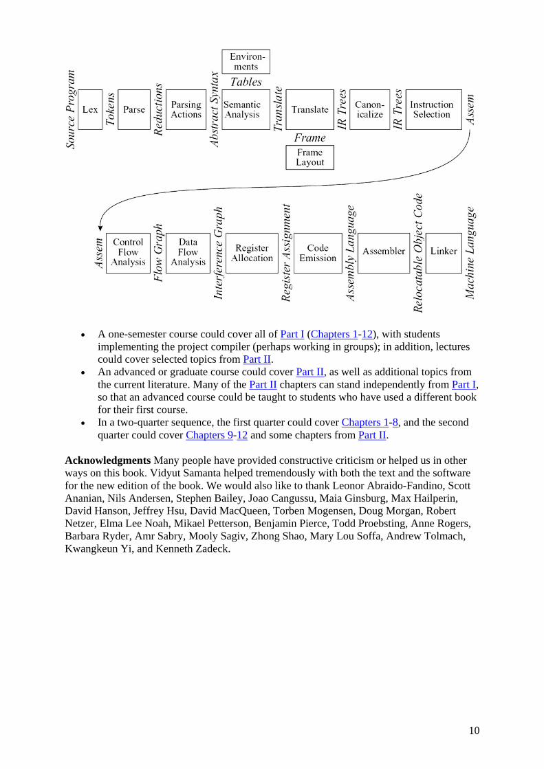
Course sequence The figure shows how the chapters depend on each other.

10

• A one-semester course could cover all of Part I (Chapters 1-12), with students implementing the project compiler (perhaps working in groups); in addition, lectures could cover selected topics from Part II.

• An advanced or graduate course could cover Part II, as well as additional topics from the current literature. Many of the Part II chapters can stand independently from Part I, so that an advanced course could be taught to students who have used a different book for their first course.

• In a two-quarter sequence, the first quarter could cover Chapters 1-8, and the second quarter could cover Chapters 9-12 and some chapters from Part II.

Acknowledgments Many people have provided constructive criticism or helped us in other ways on this book. Vidyut Samanta helped tremendously with both the text and the software for the new edition of the book. We would also like to thank Leonor Abraido-Fandino, Scott Ananian, Nils Andersen, Stephen Bailey, Joao Cangussu, Maia Ginsburg, Max Hailperin, David Hanson, Jeffrey Hsu, David MacQueen, Torben Mogensen, Doug Morgan, Robert Netzer, Elma Lee Noah, Mikael Petterson, Benjamin Pierce, Todd Proebsting, Anne Rogers, Barbara Ryder, Amr Sabry, Mooly Sagiv, Zhong Shao, Mary Lou Soffa, Andrew Tolmach, Kwangkeun Yi, and Kenneth Zadeck.

11

Part One: Fundamentals of Compilation Chapter List Chapter 1: Introduction Chapter 2: Lexical Analysis Chapter 3: Parsing Chapter 4: Abstract Syntax Chapter 5: Semantic Analysis Chapter 6: Activation Records Chapter 7: Translation to Intermediate Code Chapter 8: Basic Blocks and Traces Chapter 9: Instruction Selection Chapter 10: Liveness Analysis Chapter 11: Register Allocation Chapter 12: Putting It All Together

12

Chapter 1: Introduction A compiler was originally a program that "compiled" subroutines [a link-loader]. When in 1954 the combination "algebraic compiler" came into use, or rather into misuse, the meaning of the term had already shifted into the present one.

Bauer and Eickel [1975]

OVERVIEW

This book describes techniques, data structures, and algorithms for translating programming languages into executable code. A modern compiler is often organized into many phases, each operating on a different abstract "language." The chapters of this book follow the organization of a compiler, each covering a successive phase.

To illustrate the issues in compiling real programming languages, we show how to compile MiniJava, a simple but nontrivial subset of Java. Programming exercises in each chapter call for the implementation of the corresponding phase; a student who implements all the phases described in Part I of the book will have a working compiler. MiniJava is easily extended to support class extension or higher-order functions, and exercises in Part II show how to do this. Other chapters in Part II cover advanced techniques in program optimization. Appendix A describes the MiniJava language.

The interfaces between modules of the compiler are almost as important as the algorithms inside the modules. To describe the interfaces concretely, it is useful to write them down in a real programming language. This book uses Java - a simple object-oriented language. Java is safe, in that programs cannot circumvent the type system to violate abstractions; and it has garbage collection, which greatly simplifies the management of dynamic storage allocation. Both of these properties are useful in writing compilers (and almost any kind of software).

This is not a textbook on Java programming. Students using this book who do not know Java already should pick it up as they go along, using a Java programming book as a reference. Java is a small enough language, with simple enough concepts, that this should not be difficult for students with good programming skills in other languages.

1.1 MODULES AND INTERFACES

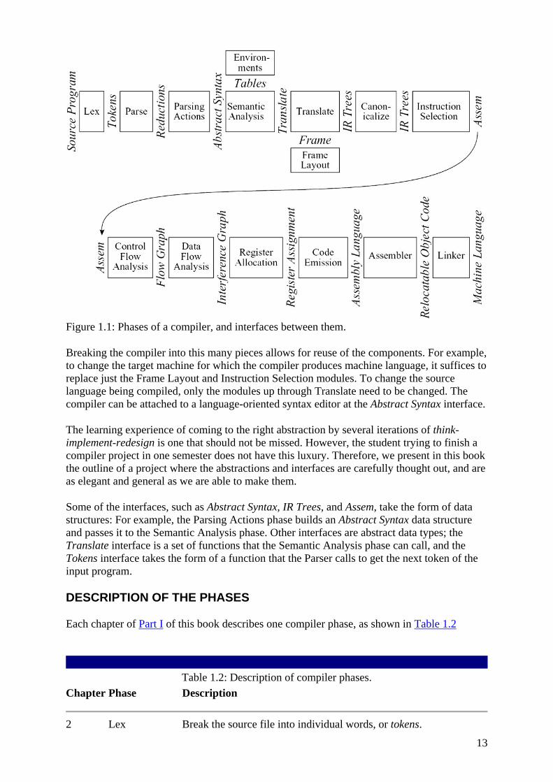
Any large software system is much easier to understand and implement if the designer takes care with the fundamental abstractions and interfaces. Figure 1.1 shows the phases in a typical compiler. Each phase is implemented as one or more software modules.

13

Figure 1.1: Phases of a compiler, and interfaces between them.

Breaking the compiler into this many pieces allows for reuse of the components. For example, to change the target machine for which the compiler produces machine language, it suffices to replace just the Frame Layout and Instruction Selection modules. To change the source language being compiled, only the modules up through Translate need to be changed. The compiler can be attached to a language-oriented syntax editor at the Abstract Syntax interface.

The learning experience of coming to the right abstraction by several iterations of think-implement-redesign is one that should not be missed. However, the student trying to finish a compiler project in one semester does not have this luxury. Therefore, we present in this book the outline of a project where the abstractions and interfaces are carefully thought out, and are as elegant and general as we are able to make them.

Some of the interfaces, such as Abstract Syntax, IR Trees, and Assem, take the form of data structures: For example, the Parsing Actions phase builds an Abstract Syntax data structure and passes it to the Semantic Analysis phase. Other interfaces are abstract data types; the Translate interface is a set of functions that the Semantic Analysis phase can call, and the Tokens interface takes the form of a function that the Parser calls to get the next token of the input program.

DESCRIPTION OF THE PHASES

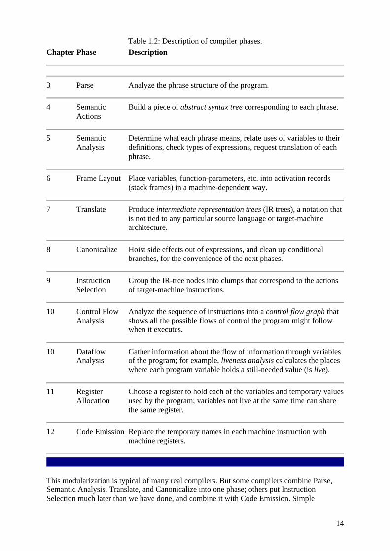
Each chapter of Part I of this book describes one compiler phase, as shown in Table 1.2

Table 1.2: Description of compiler phases. Chapter Phase Description

2 Lex Break the source file into individual words, or tokens.

14

Table 1.2: Description of compiler phases. Chapter Phase Description

3 Parse Analyze the phrase structure of the program.

4 Semantic Actions

Build a piece of abstract syntax tree corresponding to each phrase.

5 Semantic Analysis

Determine what each phrase means, relate uses of variables to their definitions, check types of expressions, request translation of each phrase.

6 Frame Layout Place variables, function-parameters, etc. into activation records (stack frames) in a machine-dependent way.

7 Translate Produce intermediate representation trees (IR trees), a notation that is not tied to any particular source language or target-machine architecture.

8 Canonicalize Hoist side effects out of expressions, and clean up conditional branches, for the convenience of the next phases.

9 Instruction Selection

Group the IR-tree nodes into clumps that correspond to the actions of target-machine instructions.

10 Control Flow Analysis

Analyze the sequence of instructions into a control flow graph that shows all the possible flows of control the program might follow when it executes.

10 Dataflow Analysis

Gather information about the flow of information through variables of the program; for example, liveness analysis calculates the places where each program variable holds a still-needed value (is live).

11 Register Allocation

Choose a register to hold each of the variables and temporary values used by the program; variables not live at the same time can share the same register.

12 Code Emission Replace the temporary names in each machine instruction with machine registers.

This modularization is typical of many real compilers. But some compilers combine Parse, Semantic Analysis, Translate, and Canonicalize into one phase; others put Instruction Selection much later than we have done, and combine it with Code Emission. Simple

15

compilers omit the Control Flow Analysis, Data Flow Analysis, and Register Allocation phases.

We have designed the compiler in this book to be as simple as possible, but no simpler. In particular, in those places where corners are cut to simplify the implementation, the structure of the compiler allows for the addition of more optimization or fancier semantics without violence to the existing interfaces.

1.2 TOOLS AND SOFTWARE

Two of the most useful abstractions used in modern compilers are contextfree grammars, for parsing, and regular expressions, for lexical analysis. To make the best use of these abstractions it is helpful to have special tools, such as Yacc (which converts a grammar into a parsing program) and Lex (which converts a declarative specification into a lexical-analysis program). Fortunately, such tools are available for Java, and the project described in this book makes use of them.

The programming projects in this book can be compiled using any Java compiler. The parser generators JavaCC and SableCC are freely available on the Internet; for information see the World Wide Web page

http://uk.cambridge.org/resources/052182060X (outside North America);

http://us.cambridge.org/titles/052182060X.html (within North America).

Source code for some modules of the MiniJava compiler, skeleton source code and support code for some of the programming exercises, example MiniJava programs, and other useful files are also available from the same Web address. The programming exercises in this book refer to this directory as $MINIJAVA/ when referring to specific subdirectories and files contained therein.

1.3 DATA STRUCTURES FOR TREE LANGUAGES

Many of the important data structures used in a compiler are intermediate representations of the program being compiled. Often these representations take the form of trees, with several node types, each of which has different attributes. Such trees can occur at many of the phase-interfaces shown in Figure 1.1.

Tree representations can be described with grammars, just like programming languages. To introduce the concepts, we will show a simple programming language with statements and expressions, but no loops or if-statements (this is called a language of straight-line programs).

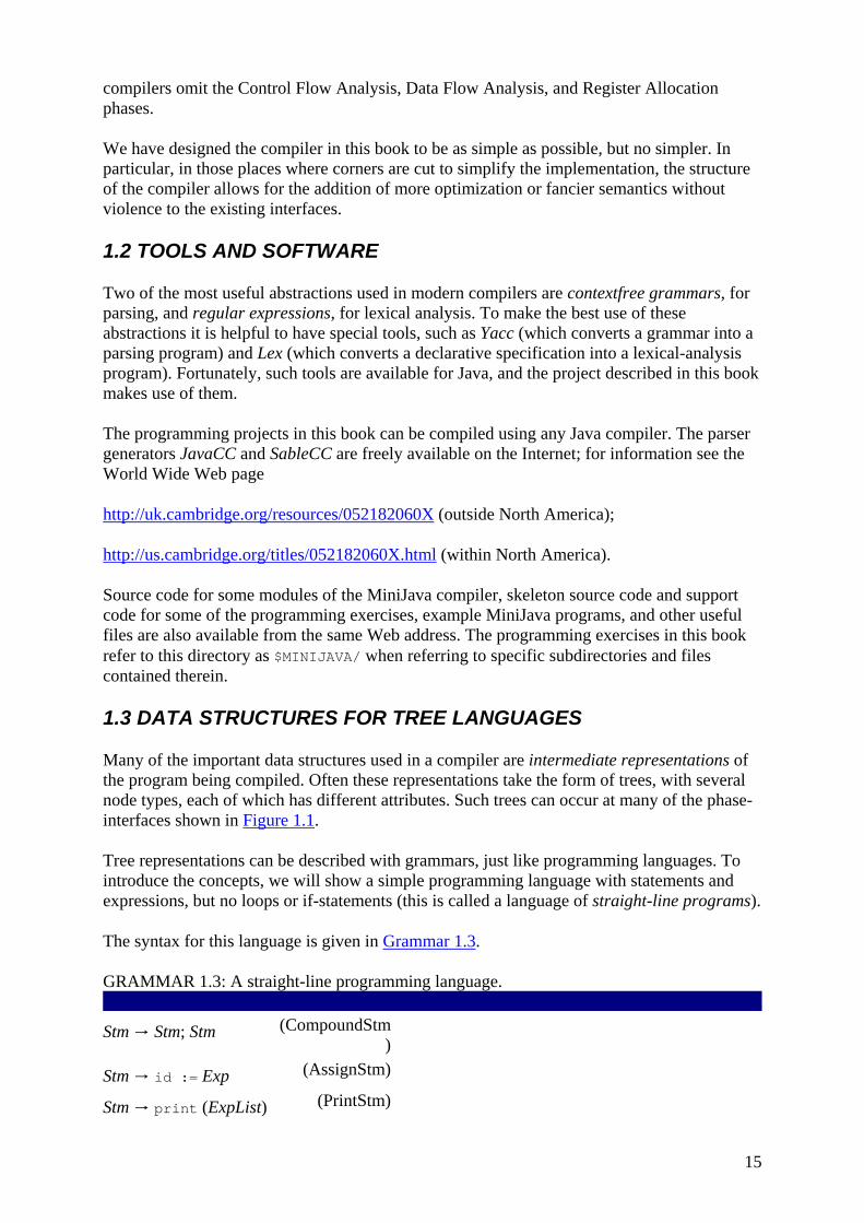
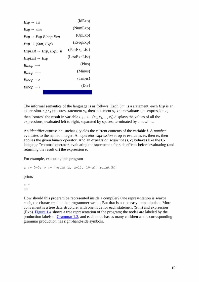
The syntax for this language is given in Grammar 1.3.

GRAMMAR 1.3: A straight-line programming language. Stm → Stm; Stm (CompoundStm

)

Stm → id := Exp (AssignStm)

Stm → print (ExpList) (PrintStm)

16

Exp → id (IdExp)

Exp → num (NumExp)

Exp → Exp Binop Exp (OpExp)

Exp → (Stm, Exp) (EseqExp)

ExpList → Exp, ExpList (PairExpList)

ExpList → Exp (LastExpList)

Binop →+ (Plus)

Binop →− (Minus)

Binop →× (Times)

Binop → / (Div)

The informal semantics of the language is as follows. Each Stm is a statement, each Exp is an expression. s1; s2 executes statement s1, then statement s2. i :=e evaluates the expression e, then "stores" the result in variable i. print(e1, e2,…, en) displays the values of all the expressions, evaluated left to right, separated by spaces, terminated by a newline.

An identifier expression, suchas i, yields the current contents of the variable i. A number evaluates to the named integer. An operator expression e1 op e2 evaluates e1, then e2, then applies the given binary operator. And an expression sequence (s, e) behaves like the C-language "comma" operator, evaluating the statement s for side effects before evaluating (and returning the result of) the expression e.

For example, executing this program

a := 5+3; b := (print(a, a-1), 10*a); print(b)

prints

8 7 80

How should this program be represented inside a compiler? One representation is source code, the characters that the programmer writes. But that is not so easy to manipulate. More convenient is a tree data structure, with one node for each statement (Stm) and expression (Exp). Figure 1.4 shows a tree representation of the program; the nodes are labeled by the production labels of Grammar 1.3, and each node has as many children as the corresponding grammar production has right-hand-side symbols.

17

Figure 1.4: Tree representation of a straight-line program.

We can translate the grammar directly into data structure definitions, as shown in Program 1.5. Each grammar symbol corresponds to an abstract class in the data structures:

Grammar class

Stm Stm Exp Exp ExpList ExpList id String num int PROGRAM 1.5: Representation of straight-line programs. public abstract class Stm {} public class CompoundStm extends Stm { public Stm stm1, stm2; public CompoundStm(Stm s1, Stm s2) {stm1=s1; stm2=s2;}} public class AssignStm extends Stm { public String id; public Exp exp; public AssignStm(String i, Exp e) {id=i; exp=e;}} public class PrintStm extends Stm { public ExpList exps; public PrintStm(ExpList e) {exps=e;}} public abstract class Exp {} public class IdExp extends Exp { public String id;

18

public IdExp(String i) {id=i;}} public class NumExp extends Exp { public int num; public NumExp(int n) {num=n;}} public class OpExp extends Exp { public Exp left, right; public int oper; final public static int Plus=1, Minus=2, Times=3, Div=4; public OpExp(Exp l, int o, Exp r) {left=l; oper=o; right=r;}} public class EseqExp extends Exp { public Stm stm; public Exp exp; public EseqExp(Stm s, Exp e) {stm=s; exp=e;}} public abstract class ExpList {} public class PairExpList extends ExpList { public Exp head; public ExpList tail; public PairExpList(Exp h, ExpList t) {head=h; tail=t;}} public class LastExpList extends ExpList { public Exp head; public LastExpList(Exp h) {head=h;}}

For each grammar rule, there is one constructor that belongs to the class for its left-hand-side symbol. We simply extend the abstract class with a "concrete" class for each grammar rule. The constructor (class) names are indicated on the right-hand side of Grammar 1.3.

Each grammar rule has right-hand-side components that must be represented in the data structures. The CompoundStm has two Stm's on the right-hand side; the AssignStm has an identifier and an expression; and so on.

These become fields of the subclasses in the Java data structure. Thus, CompoundStm has two fields (also called instance variables) called stm1 and stm2; AssignStm has fields id and exp.

For Binop we do something simpler. Although we could make a Binop class - with subclasses for Plus, Minus, Times, Div - this is overkill because none of the subclasses would need any fields. Instead we make an "enumeration" type (in Java, actually an integer) of constants (final int variables) local to the OpExp class.

Programming style We will follow several conventions for representing tree data structures in Java:

1. Trees are described by a grammar. 2. A tree is described by one or more abstract classes, each corresponding to a symbol in

the grammar. 3. Each abstract class is extended by one or more subclasses, one for each grammar rule. 4. For each nontrivial symbol in the right-hand side of a rule, there will be one field in

the corresponding class. (A trivial symbol is a punctuation symbol such as the semicolon in CompoundStm.)

5. Every class will have a constructor function that initializes all the fields. 6. Data structures are initialized when they are created (by the constructor functions), and

are never modified after that (until they are eventually discarded).

19

Modularity principles for Java programs A compiler can be a big program; careful attention to modules and interfaces prevents chaos. We will use these principles in writing a compiler in Java:

1. Each phase or module of the compiler belongs in its own package. 2. "Import on demand" declarations will not be used. If a Java file begins with 3. import A.F.*; import A.G.*; import B.*; import C.*;

then the human reader will have to look outside this file to tell which package defines the X that is used in the expression X.put().

4. "Single-type import" declarations are a better solution. If the module begins 5. import A.F.W; import A.G.X; import B.Y; import C.Z;

then you can tell without looking outside this file that X comes from A.G.

6. Java is naturally a multithreaded system. We would like to support multiple simultaneous compiler threads and compile two different programs simultaneously, one in each compiler thread. Therefore, static variables must be avoided unless they are final (constant). We never want two compiler threads to be updating the same (static) instance of a variable.

PROGRAM STRAIGHT-LINE PROGRAM INTERPRETER

Implement a simple program analyzer and interpreter for the straight-line programming language. This exercise serves as an introduction to environments (symbol tables mapping variable names to information about the variables); to abstract syntax (data structures representing the phrase structure of programs); to recursion over tree data structures, useful in many parts of a compiler; and to a functional style of programming without assignment statements.

It also serves as a "warm-up" exercise in Java programming. Programmers experienced in other languages but new to Java should be able to do this exercise, but will need supplementary material (such as textbooks) on Java.

Programs to be interpreted are already parsed into abstract syntax, as described by the data types in Program 1.5.

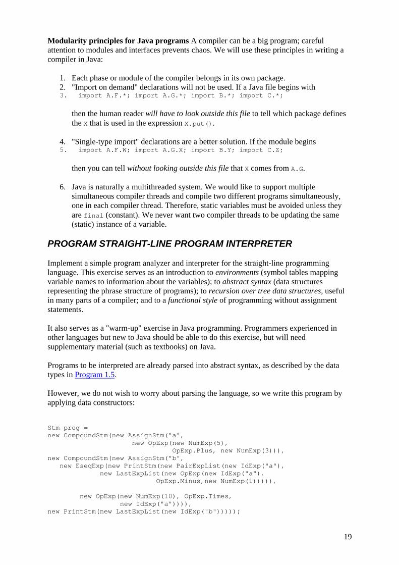
However, we do not wish to worry about parsing the language, so we write this program by applying data constructors:

Stm prog = new CompoundStm(new AssignStm("a", new OpExp(new NumExp(5), OpExp.Plus, new NumExp(3))), new CompoundStm(new AssignStm("b", new EseqExp(new PrintStm(new PairExpList(new IdExp("a"), new LastExpList(new OpExp(new IdExp("a"), OpExp.Minus,new NumExp(1))))), new OpExp(new NumExp(10), OpExp.Times, new IdExp("a")))), new PrintStm(new LastExpList(new IdExp("b")))));

20

Files with the data type declarations for the trees, and this sample program, are available in the directory $MINIJAVA/chap1.

Writing interpreters without side effects (that is, assignment statements that update variables and data structures) is a good introduction to denotational semantics and attribute grammars, which are methods for describing what programming languages do. It's often a useful technique in writing compilers, too; compilers are also in the business of saying what programming languages do.

Therefore, in implementing these programs, never assign a new value to any variable or object field except when it is initialized. For local variables, use the initializing form of declaration (for example, int i=j+3;)andfor each class, make a constructor function (like the CompoundStm constructor in Program 1.5).

1. Write a Java function int maxargs(Stm s) that tells the maximum number of arguments of any print statement within any subexpression of a given statement. For example, maxargs(prog) is 2.

2. Write a Java function void interp(Stm s) that "interprets" a program in this language. To write in a "functional programming" style - in which you never use an assignment statement - initialize each local variable as you declare it.

Your functions that examine each Exp will have to use instanceof to determine which subclass the expression belongs to and then cast to the proper subclass. Or you can add methods to the Exp and Stm classes to avoid the use of instanceof.

For part 1, remember that print statements can contain expressions that contain other print statements.

For part 2, make two mutually recursive functions interpStm and interpExp. Represent a "table", mapping identifiers to the integer values assigned to them, as a list of id × int pairs.

class Table { String id; int value; Table tail; Table(String i, int v, Table t) {id=i; value=v; tail=t;} }

Then interpStm is declared as

Table interpStm(Stm s, Table t)

taking a table t1 as argument and producing the new table t2 that's just like t1 except that some identifiers map to different integers as a result of the statement.

For example, the table t1 that maps a to 3 and maps c to 4, which we write {a ↦ 3, c ↦ 4} in mathematical notation, could be represented as the linked list .

Now, let the table t2 be just like t1, except that it maps c to 7 instead of 4. Mathematically, we could write,

t2 = update (t1, c, 7),

where the update function returns a new table {a ↦ 3, c ↦ 7}.

21

On the computer, we could implement t2 by putting a new cell at the head of the linked list: , as long as we assume that the first occurrence of c in the list

takes precedence over any later occurrence.

Therefore, the update function is easy to implement; and the corresponding lookup function

int lookup(Table t, String key)

just searches down the linked list. Of course, in an object-oriented style, int lookup(String key) should be a method of the Table class.

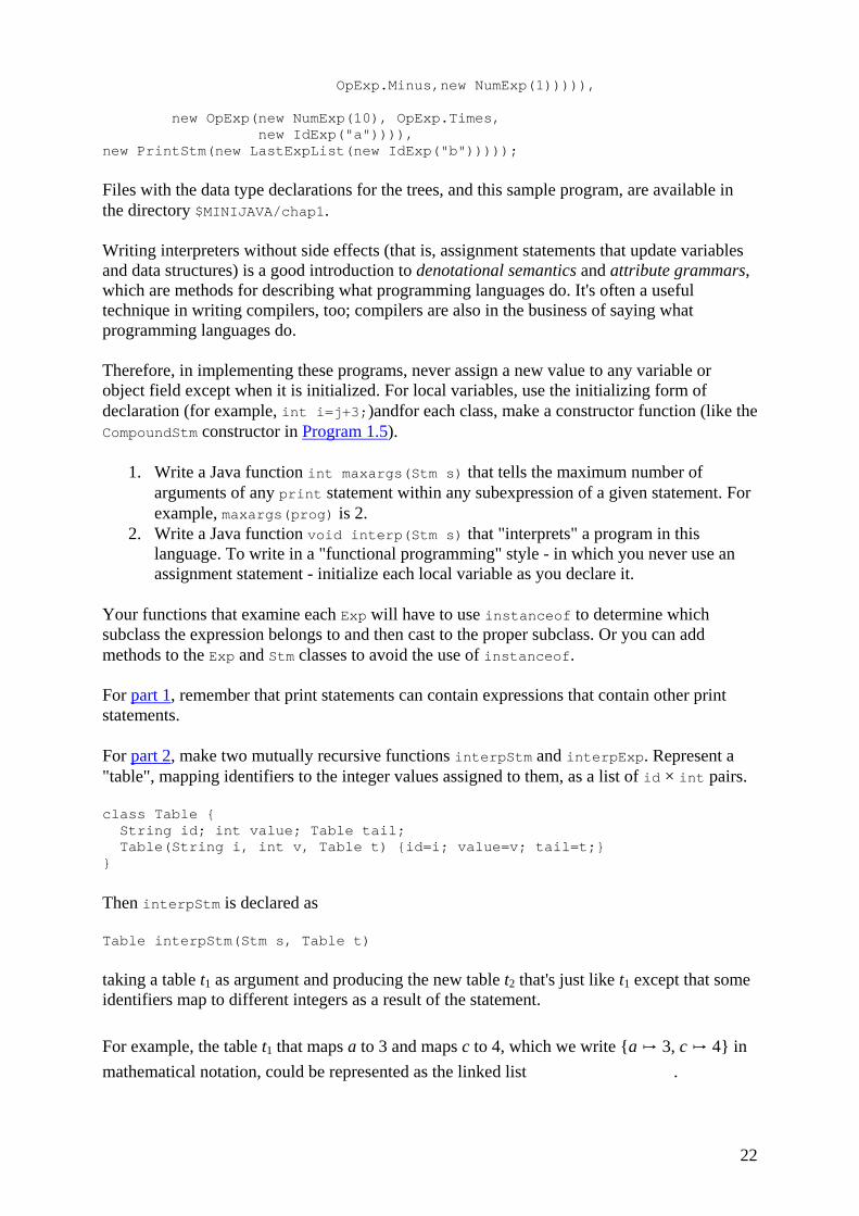
Interpreting expressions is more complicated than interpreting statements, because expressions return integer values and have side effects. We wish to simulate the straight-line programming language's assignment statements without doing any side effects in the interpreter itself. (The print statements will be accomplished by interpreter side effects, however.) The solution is to declare interpExp as

class IntAndTable {int i; Table t; IntAndTable(int ii, Table tt) {i=ii; t=tt;} }

IntAndTable interpExp(Exp e, Table t) …

The result of interpreting an expression e1 with table t1 is an integer value i and a new table t2. When interpreting an expression with two subexpressions (such as an OpExp), the table t2 resulting from the first subexpression can be used in processing the second subexpression.

PROGRAM STRAIGHT-LINE PROGRAM INTERPRETER

Implement a simple program analyzer and interpreter for the straight-line programming language. This exercise serves as an introduction to environments (symbol tables mapping variable names to information about the variables); to abstract syntax (data structures representing the phrase structure of programs); to recursion over tree data structures, useful in many parts of a compiler; and to a functional style of programming without assignment statements.

It also serves as a "warm-up" exercise in Java programming. Programmers experienced in other languages but new to Java should be able to do this exercise, but will need supplementary material (such as textbooks) on Java.

Programs to be interpreted are already parsed into abstract syntax, as described by the data types in Program 1.5.

However, we do not wish to worry about parsing the language, so we write this program by applying data constructors:

Stm prog = new CompoundStm(new AssignStm("a", new OpExp(new NumExp(5), OpExp.Plus, new NumExp(3))), new CompoundStm(new AssignStm("b", new EseqExp(new PrintStm(new PairExpList(new IdExp("a"), new LastExpList(new OpExp(new IdExp("a"),

22

OpExp.Minus,new NumExp(1))))), new OpExp(new NumExp(10), OpExp.Times, new IdExp("a")))), new PrintStm(new LastExpList(new IdExp("b")))));

Files with the data type declarations for the trees, and this sample program, are available in the directory $MINIJAVA/chap1.

Writing interpreters without side effects (that is, assignment statements that update variables and data structures) is a good introduction to denotational semantics and attribute grammars, which are methods for describing what programming languages do. It's often a useful technique in writing compilers, too; compilers are also in the business of saying what programming languages do.

Therefore, in implementing these programs, never assign a new value to any variable or object field except when it is initialized. For local variables, use the initializing form of declaration (for example, int i=j+3;)andfor each class, make a constructor function (like the CompoundStm constructor in Program 1.5).

1. Write a Java function int maxargs(Stm s) that tells the maximum number of arguments of any print statement within any subexpression of a given statement. For example, maxargs(prog) is 2.

2. Write a Java function void interp(Stm s) that "interprets" a program in this language. To write in a "functional programming" style - in which you never use an assignment statement - initialize each local variable as you declare it.

Your functions that examine each Exp will have to use instanceof to determine which subclass the expression belongs to and then cast to the proper subclass. Or you can add methods to the Exp and Stm classes to avoid the use of instanceof.

For part 1, remember that print statements can contain expressions that contain other print statements.

For part 2, make two mutually recursive functions interpStm and interpExp. Represent a "table", mapping identifiers to the integer values assigned to them, as a list of id × int pairs.

class Table { String id; int value; Table tail; Table(String i, int v, Table t) {id=i; value=v; tail=t;} }

Then interpStm is declared as

Table interpStm(Stm s, Table t)

taking a table t1 as argument and producing the new table t2 that's just like t1 except that some identifiers map to different integers as a result of the statement.

For example, the table t1 that maps a to 3 and maps c to 4, which we write {a ↦ 3, c ↦ 4} in mathematical notation, could be represented as the linked list .

23

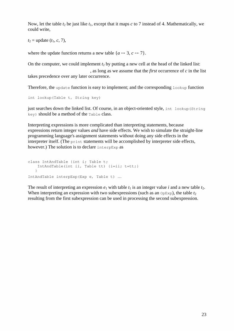
Now, let the table t2 be just like t1, except that it maps c to 7 instead of 4. Mathematically, we could write,

t2 = update (t1, c, 7),

where the update function returns a new table {a ↦ 3, c ↦ 7}.

On the computer, we could implement t2 by putting a new cell at the head of the linked list: , as long as we assume that the first occurrence of c in the list

takes precedence over any later occurrence.

Therefore, the update function is easy to implement; and the corresponding lookup function

int lookup(Table t, String key)

just searches down the linked list. Of course, in an object-oriented style, int lookup(String key) should be a method of the Table class.

Interpreting expressions is more complicated than interpreting statements, because expressions return integer values and have side effects. We wish to simulate the straight-line programming language's assignment statements without doing any side effects in the interpreter itself. (The print statements will be accomplished by interpreter side effects, however.) The solution is to declare interpExp as

class IntAndTable {int i; Table t; IntAndTable(int ii, Table tt) {i=ii; t=tt;} }

IntAndTable interpExp(Exp e, Table t) …

The result of interpreting an expression e1 with table t1 is an integer value i and a new table t2. When interpreting an expression with two subexpressions (such as an OpExp), the table t2 resulting from the first subexpression can be used in processing the second subexpression.

24

Chapter 2: Lexical Analysis lex-i-cal: of or relating to words or the vocabulary of a language as distinguished from its grammar and construction

Webster's Dictionary

OVERVIEW

To translate a program from one language into another, a compiler must first pull it apart and understand its structure and meaning, then put it together in a different way. The front end of the compiler performs analysis; the back end does synthesis.

The analysis is usually broken up into

Lexical analysis: breaking the input into individual words or "tokens";

Syntax analysis: parsing the phrase structure of the program; and

Semantic analysis: calculating the program's meaning.

The lexical analyzer takes a stream of characters and produces a stream of names, keywords, and punctuation marks; it discards white space and comments between the tokens. It would unduly complicate the parser to have to account for possible white space and comments at every possible point; this is the main reason for separating lexical analysis from parsing.

Lexical analysis is not very complicated, but we will attack it with highpowered formalisms and tools, because similar formalisms will be useful in the study of parsing and similar tools have many applications in areas other than compilation.

2.1 LEXICAL TOKENS

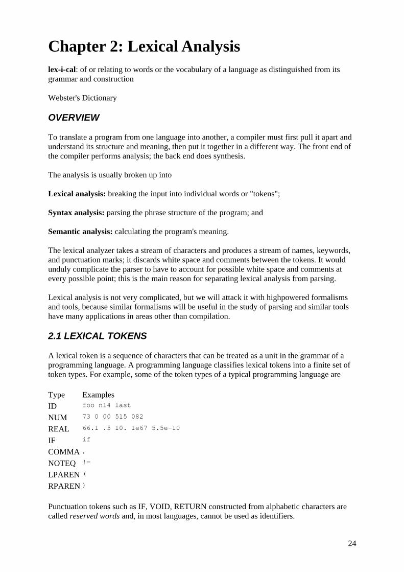
A lexical token is a sequence of characters that can be treated as a unit in the grammar of a programming language. A programming language classifies lexical tokens into a finite set of token types. For example, some of the token types of a typical programming language are

Type Examples ID foo n14 last NUM 73 0 00 515 082 REAL 66.1 .5 10. 1e67 5.5e-10

IF if COMMA , NOTEQ != LPAREN ( RPAREN )

Punctuation tokens such as IF, VOID, RETURN constructed from alphabetic characters are called reserved words and, in most languages, cannot be used as identifiers.

25

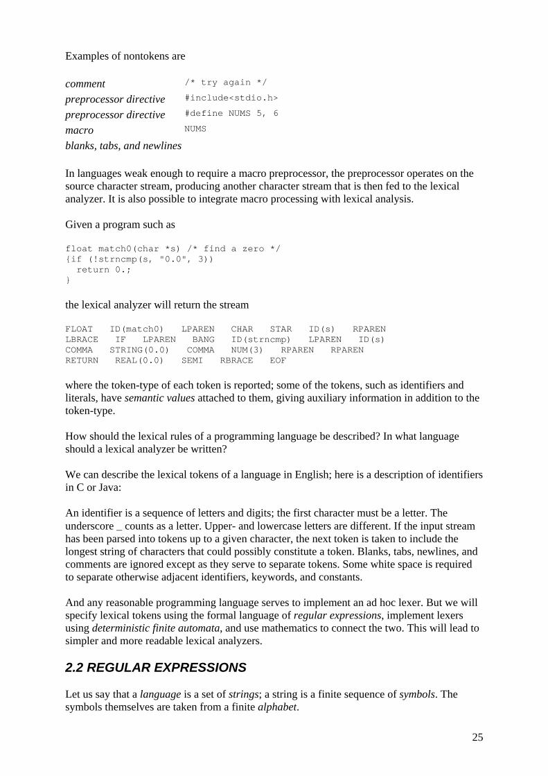
Examples of nontokens are

comment /* try again */ preprocessor directive #include<stdio.h>

preprocessor directive #define NUMS 5, 6

macro NUMS blanks, tabs, and newlines

In languages weak enough to require a macro preprocessor, the preprocessor operates on the source character stream, producing another character stream that is then fed to the lexical analyzer. It is also possible to integrate macro processing with lexical analysis.

Given a program such as

float match0(char *s) /* find a zero */ {if (!strncmp(s, "0.0", 3)) return 0.; }

the lexical analyzer will return the stream

FLOAT ID(match0) LPAREN CHAR STAR ID(s) RPAREN LBRACE IF LPAREN BANG ID(strncmp) LPAREN ID(s) COMMA STRING(0.0) COMMA NUM(3) RPAREN RPAREN RETURN REAL(0.0) SEMI RBRACE EOF

where the token-type of each token is reported; some of the tokens, such as identifiers and literals, have semantic values attached to them, giving auxiliary information in addition to the token-type.

How should the lexical rules of a programming language be described? In what language should a lexical analyzer be written?

We can describe the lexical tokens of a language in English; here is a description of identifiers in C or Java:

An identifier is a sequence of letters and digits; the first character must be a letter. The underscore _ counts as a letter. Upper- and lowercase letters are different. If the input stream has been parsed into tokens up to a given character, the next token is taken to include the longest string of characters that could possibly constitute a token. Blanks, tabs, newlines, and comments are ignored except as they serve to separate tokens. Some white space is required to separate otherwise adjacent identifiers, keywords, and constants.

And any reasonable programming language serves to implement an ad hoc lexer. But we will specify lexical tokens using the formal language of regular expressions, implement lexers using deterministic finite automata, and use mathematics to connect the two. This will lead to simpler and more readable lexical analyzers.

2.2 REGULAR EXPRESSIONS

Let us say that a language is a set of strings; a string is a finite sequence of symbols. The symbols themselves are taken from a finite alphabet.

26

The Pascal language is the set of all strings that constitute legal Pascal programs; the language of primes is the set of all decimal-digit strings that represent prime numbers; and the language of C reserved words is the set of all alphabetic strings that cannot be used as identifiers in the C programming language. The first two of these languages are infinite sets; the last is a finite set. In all of these cases, the alphabet is the ASCII character set.

When we speak of languages in this way, we will not assign any meaning to the strings; we will just be attempting to classify each string as in the language or not.

To specify some of these (possibly infinite) languages with finite descriptions, we will use the notation of regular expressions. Each regular expression stands for a set of strings.

Symbol: For each symbol a in the alphabet of the language, the regular expression a denotes the language containing just the string a.

Alternation: Given two regular expressions M and N, the alternation operator written as a vertical bar � makes a new regular expression M � N. A string is in the language of M � N if it is in the language of M or in the language of N. Thus, the language of a � b contains the two strings a and b.

Concatenation: Given two regular expressions M and N, the concatenation operator · makes a new regular expression M · N. A string is in the language of M · N if it is the concatenation of any two strings α and β such that α is in the language of M and β is in the language of N. Thus, the regular expression (a � b) · a defines the language containing the two strings aa and ba.

Epsilon: The regular expression ∊ represents a language whose only string is the empty string. Thus, (a · b) � ∊ represents the language {"", "ab"}.

Repetition: Given a regular expression M, its Kleene closure is M*. A string is in M* if it is the concatenation of zero or more strings, all of which are in M. Thus, ((a � b) · a)* represents the infinite set {"", "aa", "ba", "aaaa", "baaa", "aaba", "baba", "aaaaaa", …}.

Using symbols, alternation, concatenation, epsilon, and Kleene closure we can specify the set of ASCII characters corresponding to the lexical tokens of a programming language. First, consider some examples:

(0 | 1)* · 0 Binary numbers that are multiples of two.

b*(abb*)*(a|∊) Strings of a's and b's with no consecutive a's.

(a|b)*aa(a|b)* Strings of a's and b's containing consecutive a's.

In writing regular expressions, we will sometimes omit the concatenation symbol or the epsilon, and we will assume that Kleene closure "binds tighter" than concatenation, and concatenation binds tighter than alternation; so that ab | c means (a · b) | c, and (a |) means (a | ∊).

Let us introduce some more abbreviations: [abcd] means (a | b | c | d), [b-g] means [bcdefg], [b-gM-Qkr] means [bcdefgMNOPQkr], M? means (M | ∊), and M+ means (M·M*). These extensions are convenient, but none extend the descriptive power of regular expressions: Any

27

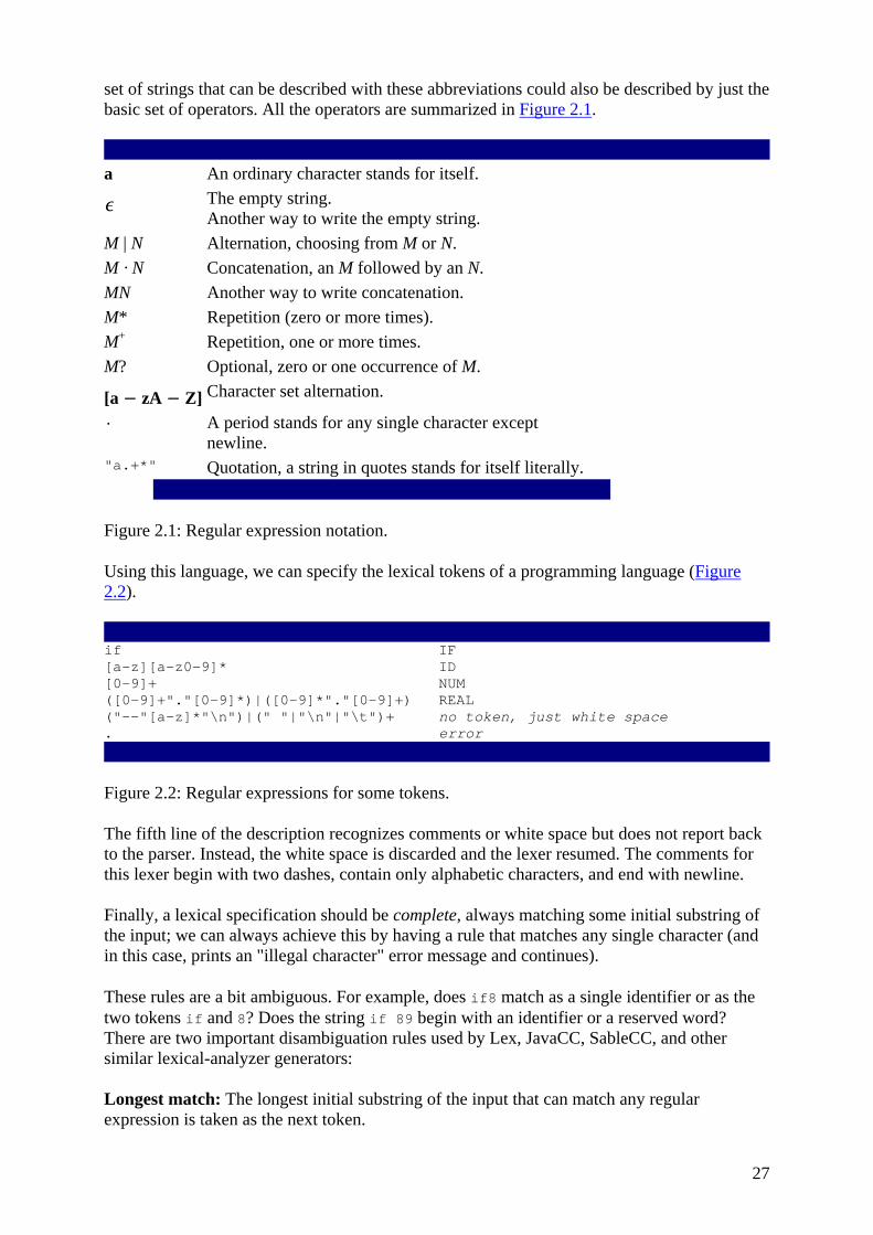
set of strings that can be described with these abbreviations could also be described by just the basic set of operators. All the operators are summarized in Figure 2.1.

a An ordinary character stands for itself.

∊ The empty string. Another way to write the empty string.

M | N Alternation, choosing from M or N. M · N Concatenation, an M followed by an N. MN Another way to write concatenation. M* Repetition (zero or more times). M+ Repetition, one or more times. M? Optional, zero or one occurrence of M.

[a − zA − Z] Character set alternation. . A period stands for any single character except

newline. "a.+*" Quotation, a string in quotes stands for itself literally.

Figure 2.1: Regular expression notation.

Using this language, we can specify the lexical tokens of a programming language (Figure 2.2).

if IF [a-z][a-z0-9]* ID [0-9]+ NUM ([0-9]+"."[0-9]*)|([0-9]*"."[0-9]+) REAL ("--"[a-z]*"\n")|(" "|"\n"|"\t")+ no token, just white space . error

Figure 2.2: Regular expressions for some tokens.

The fifth line of the description recognizes comments or white space but does not report back to the parser. Instead, the white space is discarded and the lexer resumed. The comments for this lexer begin with two dashes, contain only alphabetic characters, and end with newline.

Finally, a lexical specification should be complete, always matching some initial substring of the input; we can always achieve this by having a rule that matches any single character (and in this case, prints an "illegal character" error message and continues).

These rules are a bit ambiguous. For example, does if8 match as a single identifier or as the two tokens if and 8? Does the string if 89 begin with an identifier or a reserved word? There are two important disambiguation rules used by Lex, JavaCC, SableCC, and other similar lexical-analyzer generators:

Longest match: The longest initial substring of the input that can match any regular expression is taken as the next token.

28

Rule priority: For a particular longest initial substring, the first regular expression that can match determines its token-type. This means that the order of writing down the regular-expression rules has significance.

Thus, if8 matches as an identifier by the longest-match rule, and if matches as a reserved word by rule-priority.

2.3 FINITE AUTOMATA

Regular expressions are convenient for specifying lexical tokens, but we need a formalism that can be implemented as a computer program. For this we can use finite automata (N.B. the singular of automata is automaton). A finite automaton has a finite set of states; edges lead from one state to another, and each edge is labeled with a symbol. One state is the start state, and certain of the states are distinguished as final states.

Figure 2.3 shows some finite automata. We number the states just for convenience in discussion. The start state is numbered 1 in each case. An edge labeled with several characters is shorthand for many parallel edges; so in the ID machine there are really 26 edges each leading from state 1 to 2, each labeled by a different letter.

Figure 2.3: Finite automata for lexical tokens. The states are indicated by circles; final states are indicated by double circles. The start state has an arrow coming in from nowhere. An edge labeled with several characters is shorthand for many parallel edges.

In a deterministic finite automaton (DFA), no two edges leaving from the same state are labeled with the same symbol. A DFA accepts or rejects a string as follows. Starting in the start state, for each character in the input string the automaton follows exactly one edge to get to the next state. The edge must be labeled with the input character. After making n transitions for an n-character string, if the automaton is in a final state, then it accepts the string. If it is not in a final state, or if at some point there was no appropriately labeled edge to follow, it rejects. The language recognized by an automaton is the set of strings that it accepts.

For example, it is clear that any string in the language recognized by automaton ID must begin with a letter. Any single letter leads to state 2, which is final; so a single-letter string is accepted. From state 2, any letter or digit leads back to state 2, so a letter followed by any number of letters and digits is also accepted.

29

In fact, the machines shown in Figure 2.3 accept the same languages as the regular expressions of Figure 2.2.

These are six separate automata; how can they be combined into a single machine that can serve as a lexical analyzer? We will study formal ways of doing this in the next section, but here we will just do it ad hoc: Figure 2.4 shows such a machine. Each final state must be labeled with the token-type that it accepts. State 2 in this machine has aspects of state 2 of the IF machine and state 2 of the ID machine; since the latter is final, then the combined state must be final. State 3 is like state 3 of the IF machine and state 2 of the ID machine; because these are both final we use rule priority to disambiguate - we label state 3 with IF because we want this token to be recognized as a reserved word, not an identifier.

Figure 2.4: Combined finite automaton.

We can encode this machine as a transition matrix: a two-dimensional array (a vector of vectors), subscripted by state number and input character. There will be a "dead" state (state 0) that loops to itself on all characters; we use this to encode the absence of an edge.

int edges[][] = { /* ...012...-...e f g h i j... */ /* state 0 */ {0,0,...0,0,0...0...0,0,0,0,0,0...}, /* state 1 */ {0,0,...7,7,7...9...4,4,4,4,2,4...}, /* state 2 */ {0,0,...4,4,4...0...4,3,4,4,4,4...}, /* state 3 */ {0,0,...4,4,4...0...4,4,4,4,4,4...}, /* state 4 */ {0,0,...4,4,4...0...4,4,4,4,4,4...}, /* state 5 */ {0,0,...6,6,6...0...0,0,0,0,0,0...}, /* state 6 */ {0,0,...6,6,6...0...0,0,0,0,0,0...}, /* state 7 */ {0,0,...7,7,7...0...0,0,0,0,0,0...}, /* state 8 */ {0,0,...8,8,8...0...0,0,0,0,0,0...}, et cetera }

There must also be a "finality" array, mapping state numbers to actions - final state 2 maps to action ID, and so on.

RECOGNIZING THE LONGEST MATCH

It is easy to see how to use this table to recognize whether to accept or reject a string, but the job of a lexical analyzer is to find the longest match, the longest initial substring of the input

30

that is a valid token. While interpreting transitions, the lexer must keep track of the longest match seen so far, and the position of that match.

Keeping track of the longest match just means remembering the last time the automaton was in a final state with two variables, Last-Final (the state number of the most recent final state encountered) and Input-Position-at-Last-Final. Every time a final state is entered, the lexer updates these variables; when a dead state (a nonfinal state with no output transitions) is reached, the variables tell what token was matched, and where it ended.

Figure 2.5 shows the operation of a lexical analyzer that recognizes longest matches; note that the current input position may be far beyond the most recent position at which the recognizer was in a final state.

Figure 2.5: The automaton of Figure 2.4 recognizes several tokens. The symbol | indicates the input position at each successive call to the lexical analyzer, the symbol ⊥ indicates the current position of the automaton, and ⊺ indicates the most recent position in which the recognizer was in a final state.

2.4 NONDETERMINISTIC FINITE AUTOMATA

A nondeterministic finite automaton (NFA) is one that has a choice of edges - labeled with the same symbol - to follow out of a state. Or it may have special edges labeled with ∊ (the Greek letter epsilon) that can be followed without eating any symbol from the input.

Here is an example of an NFA:

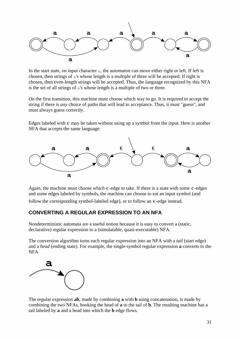
31

In the start state, on input character a, the automaton can move either right or left. If left is chosen, then strings of a's whose length is a multiple of three will be accepted. If right is chosen, then even-length strings will be accepted. Thus, the language recognized by this NFA is the set of all strings of a's whose length is a multiple of two or three.

On the first transition, this machine must choose which way to go. It is required to accept the string if there is any choice of paths that will lead to acceptance. Thus, it must "guess", and must always guess correctly.

Edges labeled with ∊ may be taken without using up a symbol from the input. Here is another NFA that accepts the same language:

Again, the machine must choose which ∊-edge to take. If there is a state with some ∊-edges and some edges labeled by symbols, the machine can choose to eat an input symbol (and follow the corresponding symbol-labeled edge), or to follow an ∊-edge instead.

CONVERTING A REGULAR EXPRESSION TO AN NFA

Nondeterministic automata are a useful notion because it is easy to convert a (static, declarative) regular expression to a (simulatable, quasi-executable) NFA.

The conversion algorithm turns each regular expression into an NFA with a tail (start edge) and a head (ending state). For example, the single-symbol regular expression a converts to the NFA

The regular expression ab, made by combining a with b using concatenation, is made by combining the two NFAs, hooking the head of a to the tail of b. The resulting machine has a tail labeled by a and a head into which the b edge flows.

32

In general, any regular expression M will have some NFA with a tail and head:

We can define the translation of regular expressions to NFAs by induction. Either an expression is primitive (a single symbol or ∊) or it is made from smaller expressions. Similarly, the NFA will be primitive or made from smaller NFAs.

Figure 2.6 shows the rules for translating regular expressions to nondeterministic automata. We illustrate the algorithm on some of the expressions in Figure 2.2 - for the tokens IF, ID, NUM, and error. Each expression is translated to an NFA, the "head" state of each NFA is marked final with a different token type, and the tails of all the expressions are joined to a new start node. The result - after some merging of equivalent NFA states - is shown in Figure 2.7.

Figure 2.6: Translation of regular expressions to NFAs.

33

Figure 2.7: Four regular expressions translated to an NFA.

CONVERTING AN NFA TO A DFA

As we saw in Section 2.3, implementing deterministic finite automata (DFAs) as computer programs is easy. But implementing NFAs is a bit harder, since most computers don't have good "guessing" hardware.

We can avoid the need to guess by trying every possibility at once. Let us simulate the NFA of Figure 2.7 on the string in. We start in state 1. Now, instead of guessing which ∊-transition to take, we just say that at this point the NFA might take any of them, so it is in one of the states {1, 4, 9, 14}; that is, we compute the ∊-closure of {1}. Clearly, there are no other states reachable without eating the first character of the input.

Now, we make the transition on the character i. From state 1 we can reach 2, from 4 we reach 5, from 9 we go nowhere, and from 14 we reach 15. So we have the set f2, 5, 15g. But again we must compute the ∊-closure: From 5 there is an ∊-transition to 8, and from 8 to 6. So the NFA must be in one of the states {2, 5, 6, 8, 15}.

On the character n, we get from state 6 to 7, from 2 to nowhere, from 5 to nowhere, from 8 to nowhere, and from 15 to nowhere. So we have the set {7}; its ∊-closure is {6, 7, 8}.

Now we are at the end of the string in; is the NFA in a final state? One of the states in our possible-states set is 8, which is final. Thus, in is an ID token.

We formally define ∊-closure as follows. Let edge(s, c) be the set of all NFA states reachable by following a single edge with label c from state s.

For a set of states S, closure(S) is the set of states that can be reached from a state in S without consuming any of the input, that is, by going only through ∊-edges. Mathematically, we can express the idea of going through ∊-edges by saying that closure(S) is the smallest set T such that

We can calculate T by iteration:

34

Why does this algorithm work? T can only grow in each iteration, so the final T must include S. If T = T′ after an iteration step, then T must also include . Finally, the algorithm must terminate, because there are only a finite number of distinct states in the NFA.

Now, when simulating an NFA as described above, suppose we are in a set d = {si; sk; sl} of NFA states si ; sk; sl. By starting in d and eating the input symbol c, we reach a new set of NFA states; we'll call this set DFAedge(d; c):

Using DFAedge, we can write the NFA simulation algorithm more formally. If the start state of the NFA is s1, and the input string is c1,…, ck, then the algorithm is

Manipulating sets of states is expensive - too costly to want to do on every character in the source program that is being lexically analyzed. But it is possible to do all the sets-of-states calculations in advance. We make a DFA from the NFA, such that each set of NFA states corresponds to one DFA state. Since the NFA has a finite number n of states, the DFA will also have a finite number (at most 2n) of states.

DFA construction is easy once we have closure and DFAedge algorithms. The DFA start state d1 is just closure(s1), as in the NFA simulation algorithm. Abstractly, there is an edge from di to dj labeled with c if dj = DFAedge(di, c). We let Σ be the alphabet.

The algorithm does not visit unreachable states of the DFA. This is extremely important, because in principle the DFA has 2n states, but in practice we usually find that only about n of them are reachable from the start state. It is important to avoid an exponential blowup in the size of the DFA interpreter's transition tables, which will form part of the working compiler.

A state d is final in the DFA if any NFA state in states[d] is final in the NFA. Labeling a state final is not enough; we must also say what token is recognized; and perhaps several members of states[d] are final in the NFA. In this case we label d with the token-type that occurred first in the list of regular expressions that constitute the lexical specification. This is how rule priority is implemented.

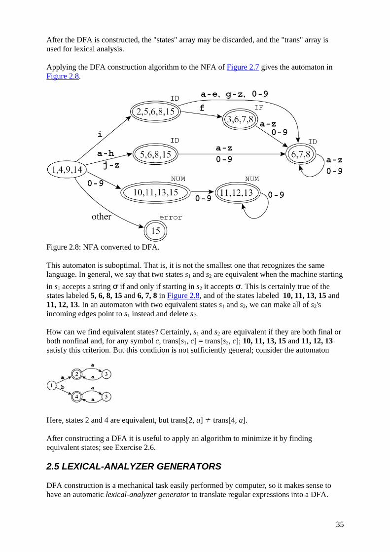
35

After the DFA is constructed, the "states" array may be discarded, and the "trans" array is used for lexical analysis.

Applying the DFA construction algorithm to the NFA of Figure 2.7 gives the automaton in Figure 2.8.

Figure 2.8: NFA converted to DFA.

This automaton is suboptimal. That is, it is not the smallest one that recognizes the same language. In general, we say that two states s1 and s2 are equivalent when the machine starting in s1 accepts a string σ if and only if starting in s2 it accepts σ. This is certainly true of the states labeled 5, 6, 8, 15 and 6, 7, 8 in Figure 2.8, and of the states labeled 10, 11, 13, 15 and 11, 12, 13. In an automaton with two equivalent states s1 and s2, we can make all of s2's incoming edges point to s1 instead and delete s2.

How can we find equivalent states? Certainly, s1 and s2 are equivalent if they are both final or both nonfinal and, for any symbol c, trans[s1, c] = trans[s2, c]; 10, 11, 13, 15 and 11, 12, 13 satisfy this criterion. But this condition is not sufficiently general; consider the automaton

Here, states 2 and 4 are equivalent, but trans[2, a] ≠ trans[4, a].

After constructing a DFA it is useful to apply an algorithm to minimize it by finding equivalent states; see Exercise 2.6.

2.5 LEXICAL-ANALYZER GENERATORS

DFA construction is a mechanical task easily performed by computer, so it makes sense to have an automatic lexical-analyzer generator to translate regular expressions into a DFA.

36

JavaCC and SableCC generate lexical analyzers and parsers written in Java. The lexical analyzers are generated from lexical specifications; and, as explained in the next chapter, the parsers are generated from grammars.

For both JavaCC and SableCC, the lexical specification and the grammar are contained in the same file.

JAVACC

The tokens described in Figure 2.2 are specified in JavaCC as shown in Program 2.9. A JavaCC specification starts with an optional list of options followed by a Java compilation unit enclosed between PARSER_BEGIN(name) and PARSER_END(name). The same name must follow PARSER_BEGIN and PARSER_END; it will be the name of the generated parser (MyParser in Program 2.9). The enclosed compilation unit must contain a class declaration of the same name as the generated parser.

PROGRAM 2.9: JavaCC specification of the tokens from Figure 2.2. PARSER_BEGIN(MyParser) class MyParser {} PARSER_END(MyParser) /* For the regular expressions on the right, the token on the left will be returned:/* TOKEN : { < IF: "if" > | < #DIGIT: ["0"-"9"] > | < ID: ["a"-"z"] (["a"-"z"]|<DIGIT>) > | < NUM: (<DIGIT>)+ > | < REAL: ( (<DIGIT>)+ "." (<DIGIT>)* ) | ( (<DIGIT>)* "." (<DIGIT>)+ )> } /* The regular expressions here will be skipped during lexical analysis: */ SKIP : { <"--" (["a"-"z"])* ("\n" | "\r" | "\r\n")> |"" | "\t" | "\n" } /* If we have a substring that does not match any of the regular expressions in TOKEN or SKIP, JavaCC will automatically throw an error. */ void Start() : {} { ( <IF> | <ID> | <NUM> | <REAL> )* }

Next is a list of grammar productions of the following kinds: a regular-expression production defines a token, a token-manager declaration can be used by the generated lexical analyzer, and two other kinds are used to define the grammar from which the parser is generated.

A lexical specification uses regular-expression productions; there are four kinds: TOKEN, SKIP, MORE, and SPECIAL_TOKEN. We will only need TOKEN and SKIP for the compiler project in this book. The kind TOKEN is used to specify that the matched string should be transformed into a token that should be communicated to the parser. The kind SKIP is used to specify that the matched string should be thrown away.

37

In Program 2.9, the specifications of ID, NUM, and REAL use the abbreviation DIGIT. The definition of DIGIT is preceeded by # to indicate that it can be used only in the definition of other tokens.

The last part of Program 2.9 begins with void Start. Itisa production which, in this case, allows the generated lexer to recognize any of the four defined tokens in any order. The next chapter will explain productions in detail.

SABLECC

The tokens described in Figure 2.2 are specified in SableCC as shown in Program 2.10. A SableCC specification file has six sections (all optional):

1. Package declaration: specifies the root package for all classes generated by SableCC. 2. Helper declarations: a list of abbreviations. 3. State declarations: support the state feature of, for example, GNU FLEX; when the

lexer is in some state, only the tokens associated with that state are recognized. States can be used for many purposes, including the detection of a beginning-of-line state, with the purpose of recognizing tokens only if they appear at the beginning of a line. For the compiler described in this book, states are not needed.

4. Token declarations: each one is used to specify that the matched string should be transformed into a token that should be communicated to the parser.

5. Ignored tokens: each one is used to specify that the matched string should be thrown away.

6. Productions: are used to define the grammar from which the parser is generated.

PROGRAM 2.10: SableCC specification of the tokens from Figure 2.2. Helpers digit = ['0'..'9']; Tokens if = 'if'; id = ['a'..'z'](['a'..'z'] | (digit))*; number = digit+; real = ((digit)+ '.' (digit)*) | ((digit)* '.' (digit)+); whitespace = (' ' | '\t' | '\n')+; comments = ('--' ['a'..'z']* '\n'); Ignored Tokens whitespace, comments;

PROGRAM LEXICAL ANALYSIS

Write the lexical-analysis part of a JavaCC or SableCC specification for MiniJava. Appendix A describes the syntax of MiniJava. The directory

$MINIJAVA/chap2/javacc

contains a test-scaffolding file Main.java that calls the lexer generated by javacc. It also contains a README file that explains how to invoke javacc. Similar files for sablecc can be found in $MINIJAVA/chap2/sablecc.

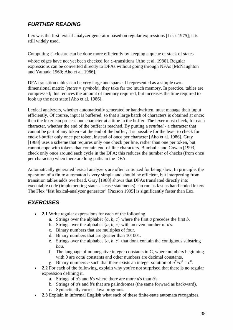
38

FURTHER READING

Lex was the first lexical-analyzer generator based on regular expressions [Lesk 1975]; it is still widely used.

Computing ∊-closure can be done more efficiently by keeping a queue or stack of states whose edges have not yet been checked for ∊-transitions [Aho et al. 1986]. Regular expressions can be converted directly to DFAs without going through NFAs [McNaughton and Yamada 1960; Aho et al. 1986].

DFA transition tables can be very large and sparse. If represented as a simple two-dimensional matrix (states × symbols), they take far too much memory. In practice, tables are compressed; this reduces the amount of memory required, but increases the time required to look up the next state [Aho et al. 1986].

Lexical analyzers, whether automatically generated or handwritten, must manage their input efficiently. Of course, input is buffered, so that a large batch of characters is obtained at once; then the lexer can process one character at a time in the buffer. The lexer must check, for each character, whether the end of the buffer is reached. By putting a sentinel - a character that cannot be part of any token - at the end of the buffer, it is possible for the lexer to check for end-of-buffer only once per token, instead of once per character [Aho et al. 1986]. Gray [1988] uses a scheme that requires only one check per line, rather than one per token, but cannot cope with tokens that contain end-of-line characters. Bumbulis and Cowan [1993] check only once around each cycle in the DFA; this reduces the number of checks (from once per character) when there are long paths in the DFA.

Automatically generated lexical analyzers are often criticized for being slow. In principle, the operation of a finite automaton is very simple and should be efficient, but interpreting from transition tables adds overhead. Gray [1988] shows that DFAs translated directly into executable code (implementing states as case statements) can run as fast as hand-coded lexers. The Flex "fast lexical-analyzer generator" [Paxson 1995] is significantly faster than Lex.

EXERCISES

• 2.1 Write regular expressions for each of the following. a. Strings over the alphabet {a, b, c} where the first a precedes the first b. b. Strings over the alphabet {a, b, c} with an even number of a's. c. Binary numbers that are multiples of four. d. Binary numbers that are greater than 101001. e. Strings over the alphabet {a, b, c} that don't contain the contiguous substring

baa. f. The language of nonnegative integer constants in C, where numbers beginning

with 0 are octal constants and other numbers are decimal constants. g. Binary numbers n such that there exists an integer solution of an+bn = cn.

• 2.2 For each of the following, explain why you're not surprised that there is no regular expression defining it.

a. Strings of a's and b's where there are more a's than b's. b. Strings of a's and b's that are palindromes (the same forward as backward). c. Syntactically correct Java programs.

• 2.3 Explain in informal English what each of these finite-state automata recognizes.

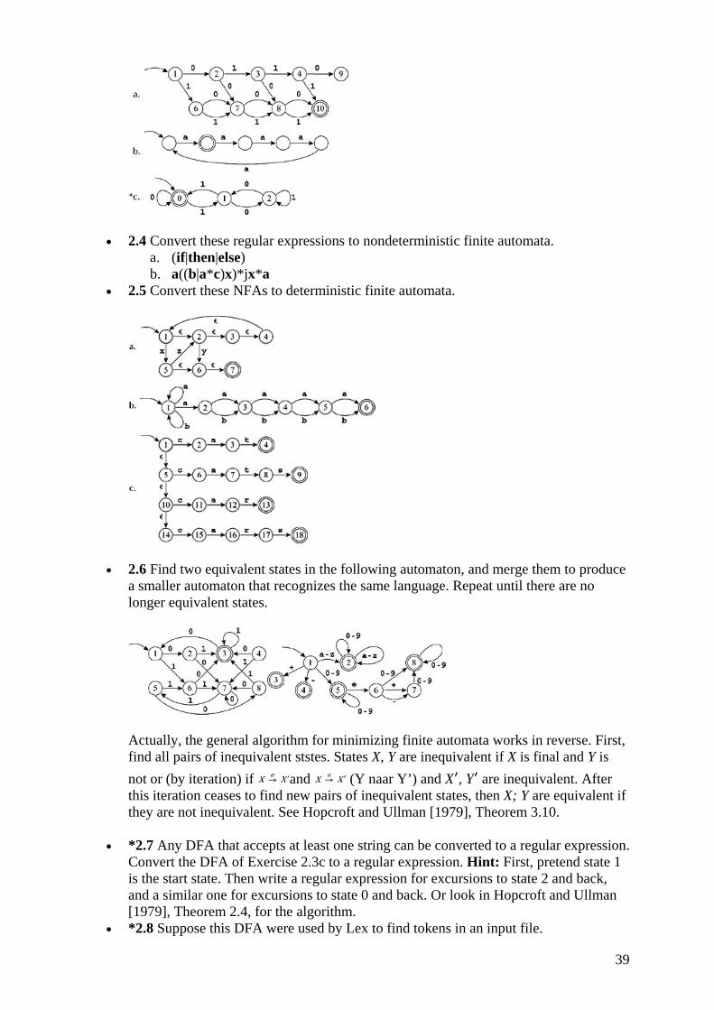
39

• 2.4 Convert these regular expressions to nondeterministic finite automata. a. (if|then|else) b. a((b|a*c)x)*jx*a

• 2.5 Convert these NFAs to deterministic finite automata.

• 2.6 Find two equivalent states in the following automaton, and merge them to produce a smaller automaton that recognizes the same language. Repeat until there are no longer equivalent states.

Actually, the general algorithm for minimizing finite automata works in reverse. First, find all pairs of inequivalent ststes. States X, Y are inequivalent if X is final and Y is not or (by iteration) if and (Y naar Y’) and X′, Y′ are inequivalent. After this iteration ceases to find new pairs of inequivalent states, then X; Y are equivalent if they are not inequivalent. See Hopcroft and Ullman [1979], Theorem 3.10.

• *2.7 Any DFA that accepts at least one string can be converted to a regular expression. Convert the DFA of Exercise 2.3c to a regular expression. Hint: First, pretend state 1 is the start state. Then write a regular expression for excursions to state 2 and back, and a similar one for excursions to state 0 and back. Or look in Hopcroft and Ullman [1979], Theorem 2.4, for the algorithm.

• *2.8 Suppose this DFA were used by Lex to find tokens in an input file.

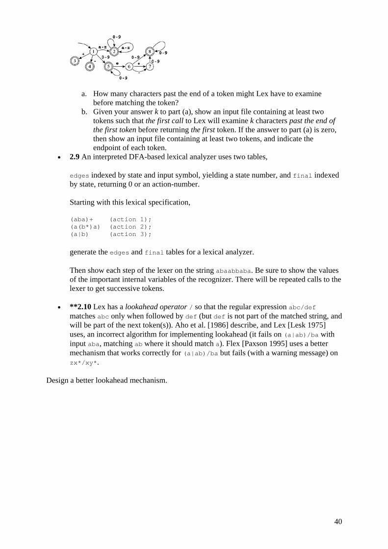
40

a. How many characters past the end of a token might Lex have to examine before matching the token?

b. Given your answer k to part (a), show an input file containing at least two tokens such that the first call to Lex will examine k characters past the end of the first token before returning the first token. If the answer to part (a) is zero, then show an input file containing at least two tokens, and indicate the endpoint of each token.

• 2.9 An interpreted DFA-based lexical analyzer uses two tables,

edges indexed by state and input symbol, yielding a state number, and final indexed by state, returning 0 or an action-number.

Starting with this lexical specification,

(aba)+ (action 1); (a(b*)a) (action 2); (a|b) (action 3);

generate the edges and final tables for a lexical analyzer.

Then show each step of the lexer on the string abaabbaba. Be sure to show the values of the important internal variables of the recognizer. There will be repeated calls to the lexer to get successive tokens.

• **2.10 Lex has a lookahead operator / so that the regular expression abc/def matches abc only when followed by def (but def is not part of the matched string, and will be part of the next token(s)). Aho et al. [1986] describe, and Lex [Lesk 1975] uses, an incorrect algorithm for implementing lookahead (it fails on (a|ab)/ba with input aba, matching ab where it should match a). Flex [Paxson 1995] uses a better mechanism that works correctly for (a|ab)/ba but fails (with a warning message) on zx*/xy*.

Design a better lookahead mechanism.

41

Chapter 3: Parsing syn-tax: the way in which words are put together to form phrases, clauses, or sentences.


OVERVIEW

The abbreviation mechanism discussed in the previous chapter, whereby a symbol stands for some regular expression, is convenient enough that it is tempting to use it in interesting ways:

These regular expressions define sums of the form 28+301+9.

But now consider

This is meant to define expressions of the form:

(109+23) 61 (1+(250+3))

in which all the parentheses are balanced. But it is impossible for a finite automaton to recognize balanced parentheses (because a machine with N states cannot remember a parenthesis-nesting depth greater than N), so clearly sum and expr cannot be regular expressions.

So how does a lexical analyzer implement regular-expression abbreviations such as digits? The answer is that the right-hand-side ([0-9]+) is simply substituted for digits wherever it appears in regular expressions, before translation to a finite automaton.

This is not possible for the sum-and-expr language; we can first substitute sum into expr, yielding

but now an attempt to substitute expr into itself leads to

and the right-hand side now has just as many occurrences of expr as it did before - in fact, it has more!

Thus, the notion of abbreviation does not add expressive power to the language of regular expressions - there are no additional languages that can be defined - unless the abbreviations are recursive (or mutually recursive, as are sum and expr).

42

The additional expressive power gained by recursion is just what we need for parsing. Also, once we have abbreviations with recursion, we do not need alternation except at the top level of expressions, because the definition

can always be rewritten using an auxiliary definition as

In fact, instead of using the alternation mark at all, we can just write several allowable expansions for the same symbol:

The Kleene closure is not necessary, since we can rewrite it so that

becomes

What we have left is a very simple notation, called context-free grammars. Just as regular expressions can be used to define lexical structure in a static, declarative way, grammars define syntactic structure declaratively. But we will need something more powerful than finite automata to parse languages described by grammars.

In fact, grammars can also be used to describe the structure of lexical tokens, although regular expressions are adequate - and more concise - for that purpose.

3.1 CONTEXT-FREE GRAMMARS

As before, we say that a language is a set of strings; each string is a finite sequence of symbols taken from a finite alphabet. For parsing, the strings are source programs, the symbols are lexical tokens, and the alphabet is the set of token-types returned by the lexical analyzer.

A context-free grammar describes a language. A grammar has a set of productions of the form

symbol → symbol symbol … symbol

where there are zero or more symbols on the right-hand side. Each symbol is either terminal, meaning that it is a token from the alphabet of strings in the language, or nonterminal, meaning that it appears on the left-hand side of some production. No token can ever appear on the left-hand side of a production. Finally, one of the nonterminals is distinguished as the start symbol of the grammar.

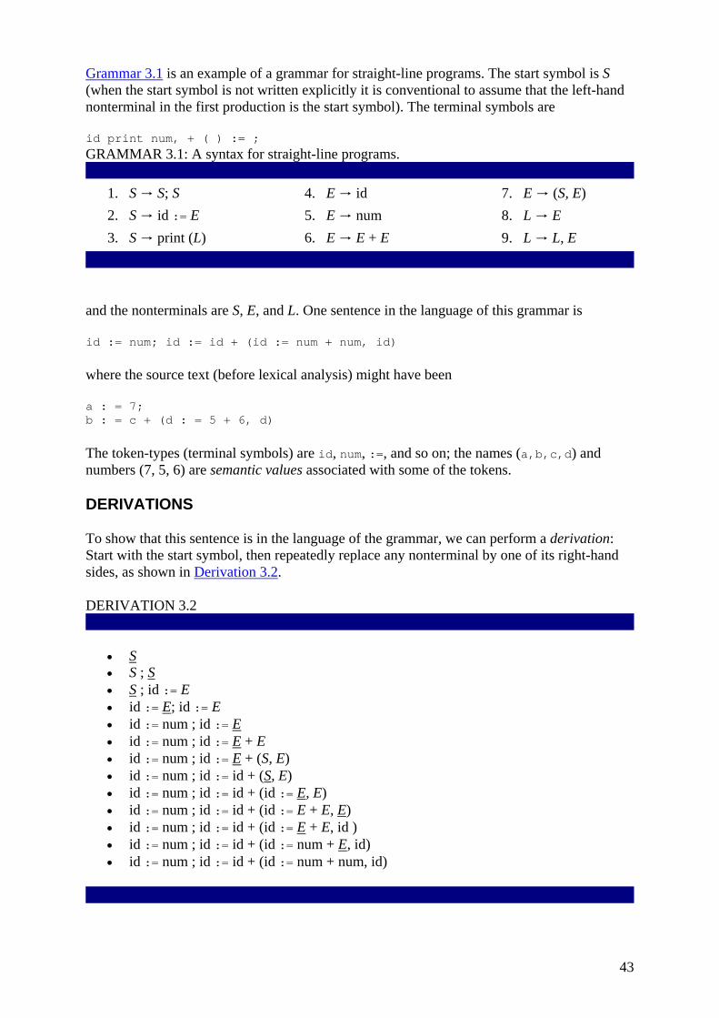
43

Grammar 3.1 is an example of a grammar for straight-line programs. The start symbol is S (when the start symbol is not written explicitly it is conventional to assume that the left-hand nonterminal in the first production is the start symbol). The terminal symbols are

id print num, + ( ) := ; GRAMMAR 3.1: A syntax for straight-line programs.

1. S → S; S 2. S → id := E 3. S → print (L)

4. E → id 5. E → num 6. E → E + E

7. E → (S, E) 8. L → E 9. L → L, E

and the nonterminals are S, E, and L. One sentence in the language of this grammar is

id := num; id := id + (id := num + num, id)

where the source text (before lexical analysis) might have been

a : = 7; b : = c + (d : = 5 + 6, d)

The token-types (terminal symbols) are id, num, :=, and so on; the names (a,b,c,d) and numbers (7, 5, 6) are semantic values associated with some of the tokens.

DERIVATIONS

To show that this sentence is in the language of the grammar, we can perform a derivation: Start with the start symbol, then repeatedly replace any nonterminal by one of its right-hand sides, as shown in Derivation 3.2.

DERIVATION 3.2

• S • S ; S • S ; id := E • id := E; id := E • id := num ; id := E • id := num ; id := E + E • id := num ; id := E + (S, E) • id := num ; id := id + (S, E) • id := num ; id := id + (id := E, E) • id := num ; id := id + (id := E + E, E) • id := num ; id := id + (id := E + E, id ) • id := num ; id := id + (id := num + E, id) • id := num ; id := id + (id := num + num, id)

44

There are many different derivations of the same sentence. A leftmost derivation is one in which the leftmost nonterminal symbol is always the one expanded; in a rightmost derivation, the rightmost nonterminal is always the next to be expanded.

Derivation 3.2 is neither leftmost nor rightmost; a leftmost derivation for this sentence would begin,

• S • S ; S • id := E ; S • id := num ; S • id := num ; id := E • id := num ; id := E + E • ⋮

PARSE TREES

A parse tree is made by connecting each symbol in a derivation to the one from which it was derived, as shown in Figure 3.3. Two different derivations can have the same parse tree.

Figure 3.3: Parse tree.

AMBIGUOUS GRAMMARS

A grammar is ambiguous if it can derive a sentence with two different parse trees. Grammar 3.1 is ambiguous, since the sentence id := id+id+id has two parse trees (Figure 3.4).

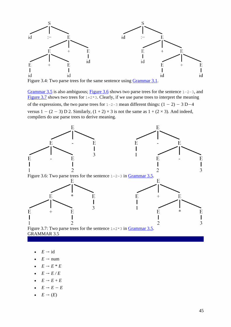
45

Figure 3.4: Two parse trees for the same sentence using Grammar 3.1.

Grammar 3.5 is also ambiguous; Figure 3.6 shows two parse trees for the sentence 1-2-3, and Figure 3.7 shows two trees for 1+2*3. Clearly, if we use parse trees to interpret the meaning of the expressions, the two parse trees for 1-2-3 mean different things: (1 − 2) − 3 D−4 versus 1 − (2 − 3) D 2. Similarly, (1 + 2) × 3 is not the same as 1 + (2 × 3). And indeed, compilers do use parse trees to derive meaning.

Figure 3.6: Two parse trees for the sentence 1-2-3 in Grammar 3.5.

Figure 3.7: Two parse trees for the sentence 1+2*3 in Grammar 3.5. GRAMMAR 3.5

• E → id • E → num • E → E * E • E → E / E • E → E + E • E → E − E • E → (E)

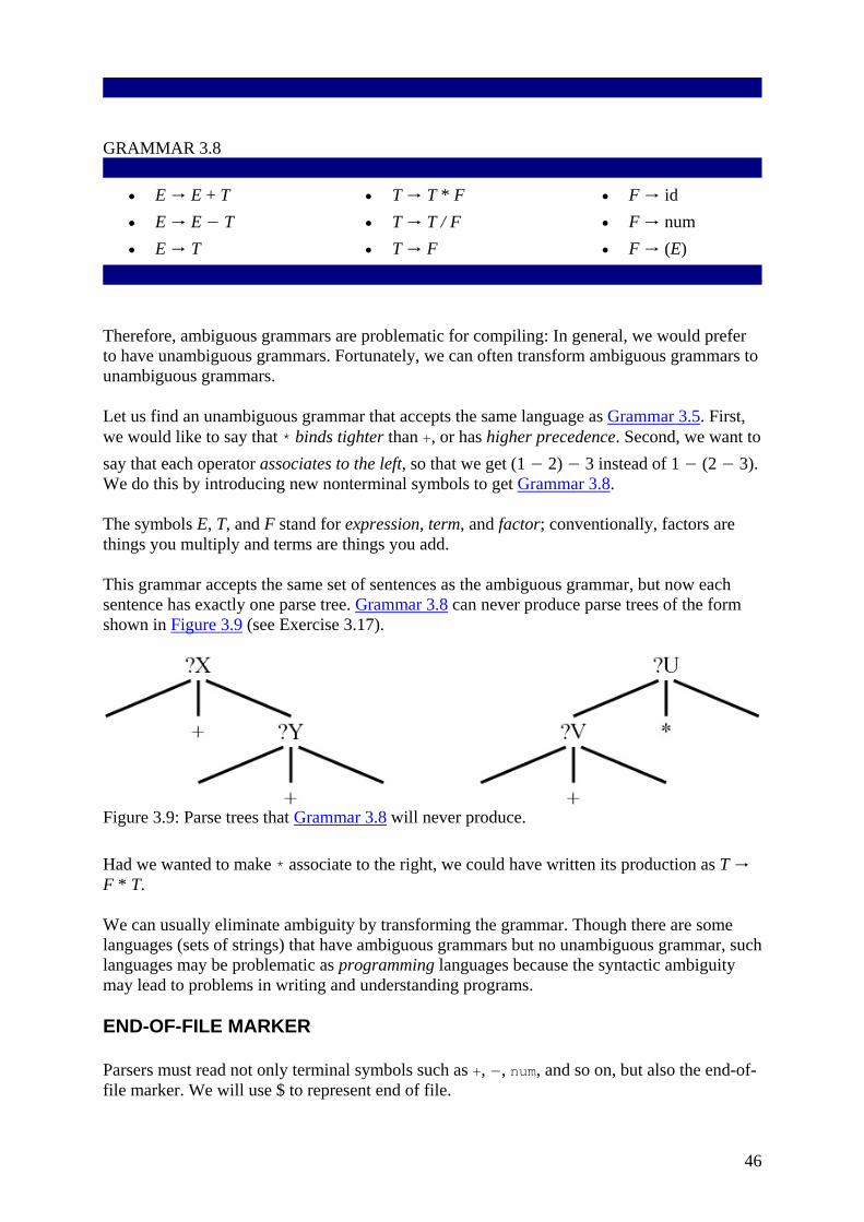
46

GRAMMAR 3.8

• E → E + T • E → E − T • E → T

• T → T * F • T → T / F • T → F

• F → id • F → num • F → (E)

Therefore, ambiguous grammars are problematic for compiling: In general, we would prefer to have unambiguous grammars. Fortunately, we can often transform ambiguous grammars to unambiguous grammars.

Let us find an unambiguous grammar that accepts the same language as Grammar 3.5. First, we would like to say that * binds tighter than +, or has higher precedence. Second, we want to say that each operator associates to the left, so that we get (1 − 2) − 3 instead of 1 − (2 − 3). We do this by introducing new nonterminal symbols to get Grammar 3.8.

The symbols E, T, and F stand for expression, term, and factor; conventionally, factors are things you multiply and terms are things you add.

This grammar accepts the same set of sentences as the ambiguous grammar, but now each sentence has exactly one parse tree. Grammar 3.8 can never produce parse trees of the form shown in Figure 3.9 (see Exercise 3.17).

Figure 3.9: Parse trees that Grammar 3.8 will never produce.

Had we wanted to make * associate to the right, we could have written its production as T → F * T.

We can usually eliminate ambiguity by transforming the grammar. Though there are some languages (sets of strings) that have ambiguous grammars but no unambiguous grammar, such languages may be problematic as programming languages because the syntactic ambiguity may lead to problems in writing and understanding programs.

END-OF-FILE MARKER

Parsers must read not only terminal symbols such as +, −, num, and so on, but also the end-of-file marker. We will use $ to represent end of file.

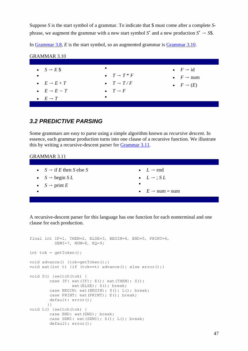
47

Suppose S is the start symbol of a grammar. To indicate that $ must come after a complete S-phrase, we augment the grammar with a new start symbol S′ and a new production S′ → S$.

In Grammar 3.8, E is the start symbol, so an augmented grammar is Grammar 3.10.

GRAMMAR 3.10

• S → E $ • • E → E + T • E → E − T • E → T

• • T → T * F • T → T / F • T → F •

• F → id • F → num • F → (E)

3.2 PREDICTIVE PARSING

Some grammars are easy to parse using a simple algorithm known as recursive descent. In essence, each grammar production turns into one clause of a recursive function. We illustrate this by writing a recursive-descent parser for Grammar 3.11.

GRAMMAR 3.11

• S → if E then S else S • S → begin S L • S → print E •

• L → end • L → ; S L • • E → num = num

A recursive-descent parser for this language has one function for each nonterminal and one clause for each production.

final int IF=1, THEN=2, ELSE=3, BEGIN=4, END=5, PRINT=6, SEMI=7, NUM=8, EQ=9; int tok = getToken(); void advance() {tok=getToken();} void eat(int t) {if (tok==t) advance(); else error();} void S() {switch(tok) { case IF: eat(IF); E(); eat(THEN); S(); eat(ELSE); S(); break; case BEGIN: eat(BEGIN); S(); L(); break; case PRINT: eat(PRINT); E(); break; default: error(); }} void L() {switch(tok) { case END: eat(END); break; case SEMI: eat(SEMI); S(); L(); break; default: error();

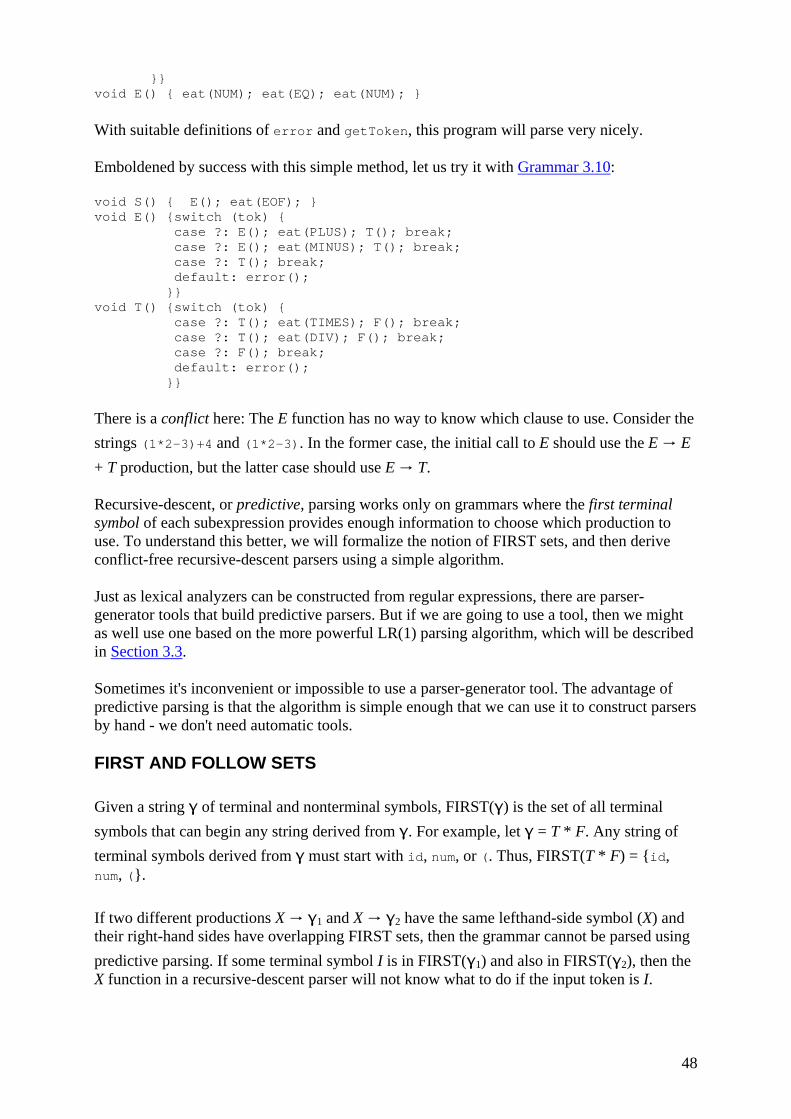
48

}} void E() { eat(NUM); eat(EQ); eat(NUM); }

With suitable definitions of error and getToken, this program will parse very nicely.

Emboldened by success with this simple method, let us try it with Grammar 3.10:

void S() { E(); eat(EOF); } void E() {switch (tok) { case ?: E(); eat(PLUS); T(); break; case ?: E(); eat(MINUS); T(); break; case ?: T(); break; default: error(); }} void T() {switch (tok) { case ?: T(); eat(TIMES); F(); break; case ?: T(); eat(DIV); F(); break; case ?: F(); break; default: error(); }}

There is a conflict here: The E function has no way to know which clause to use. Consider the strings (1*2-3)+4 and (1*2-3). In the former case, the initial call to E should use the E → E + T production, but the latter case should use E → T.

Recursive-descent, or predictive, parsing works only on grammars where the first terminal symbol of each subexpression provides enough information to choose which production to use. To understand this better, we will formalize the notion of FIRST sets, and then derive conflict-free recursive-descent parsers using a simple algorithm.

Just as lexical analyzers can be constructed from regular expressions, there are parser-generator tools that build predictive parsers. But if we are going to use a tool, then we might as well use one based on the more powerful LR(1) parsing algorithm, which will be described in Section 3.3.

Sometimes it's inconvenient or impossible to use a parser-generator tool. The advantage of predictive parsing is that the algorithm is simple enough that we can use it to construct parsers by hand - we don't need automatic tools.

FIRST AND FOLLOW SETS

Given a string γ of terminal and nonterminal symbols, FIRST(γ) is the set of all terminal symbols that can begin any string derived from γ. For example, let γ = T * F. Any string of terminal symbols derived from γ must start with id, num, or (. Thus, FIRST(T * F) = {id, num, (}.

If two different productions X → γ1 and X → γ2 have the same lefthand-side symbol (X) and their right-hand sides have overlapping FIRST sets, then the grammar cannot be parsed using predictive parsing. If some terminal symbol I is in FIRST(γ1) and also in FIRST(γ2), then the X function in a recursive-descent parser will not know what to do if the input token is I.

49

The computation of FIRST sets looks very simple: If γ = X Y Z, it seems as if Y and Z can be ignored, and FIRST(X) is the only thing that matters. But consider Grammar 3.12. Because Y can produce the empty string - and therefore X can produce the empty string - we find that FIRST(X Y Z) must include FIRST(Z). Therefore, in computing FIRST sets, we must keep track of which symbols can produce the empty string; we say such symbols are nullable. And we must keep track of what might follow a nullable symbol.

GRAMMAR 3.12

• Z → d • Z → X Y Z

• Y → • Y → c

• X → Y • X → a

With respect to a particular grammar, given a string γ of terminals and nonterminals,

• nullable(X) is true if X can derive the empty string. • FIRST(γ) is the set of terminals that can begin strings derived from γ. • FOLLOW(X) is the set of terminals that can immediately follow X. That is, t ∈

FOLLOW(X) if there is any derivation containing Xt. This can occur if the derivation contains X Y Zt where Y and Z both derive ∊.

A precise definition of FIRST, FOLLOW, and nullable is that they are the smallest sets for which these properties hold:

For each terminal symbol Z, FIRST[Z] = {Z}.

Algorithm 3.13 for computing FIRST, FOLLOW, and nullable just follows from these facts; we simply replace each equation with an assignment statement, and iterate.

ALGORITHM 3.13: Iterative computation of FIRST, FOLLOW, and nullable.

Algorithm to compute FIRST, FOLLOW, and nullable.

Initialize FIRST and FOLLOW to all empty sets, and nullable to all false.

for each terminal symbol Z

FIRST[Z] ← {Z} repeat

50

for each production X → Y1Y2 ... Yk if Y1 ... Yk are all nullable (or if k = 0)

then nullable[X] ← true for each i from 1 to k, each j from i + 1 to k if Y1 ... Yi-1 are all nullable (or if i = 1)

then FIRST[X] ← FIRST[X] ∪ FIRST[Yi ] if Yi+1 ... Yk are all nullable (or if i = k)

then FOLLOW[Yi] ← FOLLOW[Yi] ∪ FOLLOW[X] if Yi+1 ... Yj -1 are all nullable (or if i + 1 = j)

then FOLLOW[Yi] ← FOLLOW[Yi] ∪ FIRST[Yj] until FIRST, FOLLOW, and nullable did not change in this iteration.

Of course, to make this algorithm efficient it helps to examine the productions in the right order; see Section 17.4. Also, the three relations need not be computed simultaneously; nullable can be computed by itself, then FIRST, then FOLLOW.

This is not the first time that a group of equations on sets has become the algorithm for calculating those sets; recall the algorithm on page 28 for computing ∊-closure. Nor will it be the last time; the technique of iteration to a fixed point is applicable in dataflow analysis for optimization, in the back end of a compiler.

We can apply this algorithm to Grammar 3.12. Initially, we have:

In the first iteration, we find that a ∈ FIRST[X], Y is nullable, c ∈ FIRST[Y], d ∈ FIRST[Z], d ∈ FOLLOW[X], c ∈ FOLLOW[X], d ∈ FOLLOW[Y]. Thus:

In the second iteration, we find that X is nullable, c ∈ FIRST[X], {a; c} ⊆ FIRST[Z], {a, c, d} ⊆ FOLLOW[X], {a, c, d} ⊆ FOLLOW[Y]. Thus:

The third iteration finds no new information, and the algorithm terminates.

It is useful to generalize the FIRST relation to strings of symbols:

FIRST(Xγ) = FIRST[X] if not nullable[X]

FIRST(Xγ) = FIRST[X] ∪ FIRST(γ) if nullable[X]

and similarly, we say that a string γ is nullable if each symbol in γ is nullable.

51

CONSTRUCTING A PREDICTIVE PARSER

Consider a recursive-descent parser. The parsing function for some nonterminal X has a clause for each X production; it must choose one of these clauses based on the next token T of the input. If we can choose the right production for each (X, T), then we can write the recursive-descent parser. All the information we need can be encoded as a two-dimensional table of productions, indexed by nonterminals X and terminals T. Thisiscalleda predictive parsing table.

To construct this table, enter production X → γ in row X, column T of the table for each T ∈ FIRST(γ). Also, if γ is nullable, enter the production in row X, column T for each T ∈ FOLLOW[X].

Figure 3.14 shows the predictive parser for Grammar 3.12. But some of the entries contain more than one production! The presence of duplicate entries means that predictive parsing will not work on Grammar 3.12.

Figure 3.14: Predictive parsing table for Grammar 3.12.

If we examine the grammar more closely, we find that it is ambiguous. The sentence d has many parse trees, including:

An ambiguous grammar will always lead to duplicate entries in a predictive parsing table. If we need to use the language of Grammar 3.12 as a programming language, we will need to find an unambiguous grammar.

Grammars whose predictive parsing tables contain no duplicate entries are called LL(1). This stands for left-to-right parse, leftmost-derivation, 1-symbol lookahead. Clearly a recursive-descent (predictive) parser examines the input left-to-right in one pass (some parsing algorithms do not, but these are generally not useful for compilers). The order in which a predictive parser expands nonterminals into right-hand sides (that is, the recursive-descent parser calls functions corresponding to nonterminals) is just the order in which a leftmost derivation expands nonterminals. And a recursive-descent parser does its job just by looking at the next token of the input, never looking more than one token ahead.

52

We can generalize the notion of FIRST sets to describe the first k tokens of a string, and to make an LL(k) parsing table whose rows are the nonterminals and columns are every sequence of k terminals. This is rarely done (because the tables are so large), but sometimes when you write a recursive-descent parser by hand you need to look more than one token ahead.

Grammars parsable with LL(2) parsing tables are called LL(2) grammars, and similarly for LL(3), etc. Every LL(1) grammar is an LL(2) grammar, and so on. No ambiguous grammar is LL(k)forany k.

ELIMINATING LEFT RECURSION

Suppose we want to build a predictive parser for Grammar 3.10. The two productions

are certain to cause duplicate entries in the LL(1) parsing table, since any token in FIRST(T) will also be in FIRST(E + T). The problem is that E appears as the first right-hand-side symbol in an E-production; this is called left recursion. Grammars with left recursion cannot be LL(1).

To eliminate left recursion, we will rewrite using right recursion. We introduce a new nonterminal E′, and write

This derives the same set of strings (on T and +) as the original two productions, but now there is no left recursion.

In general, whenever we have productions X → Xγ and X → α, where α does not start with X, we know that this derives strings of the form αγ*, an α followed by zero or more γ. So we can rewrite the regular expression using right recursion:

Applying this transformation to Grammar 3.10, we obtain Grammar 3.15.

GRAMMAR 3.15

• S → E $ • • E → T E′

• • E′ → + T E′ • E′ →− T E′

• E′ → • • T → F T′

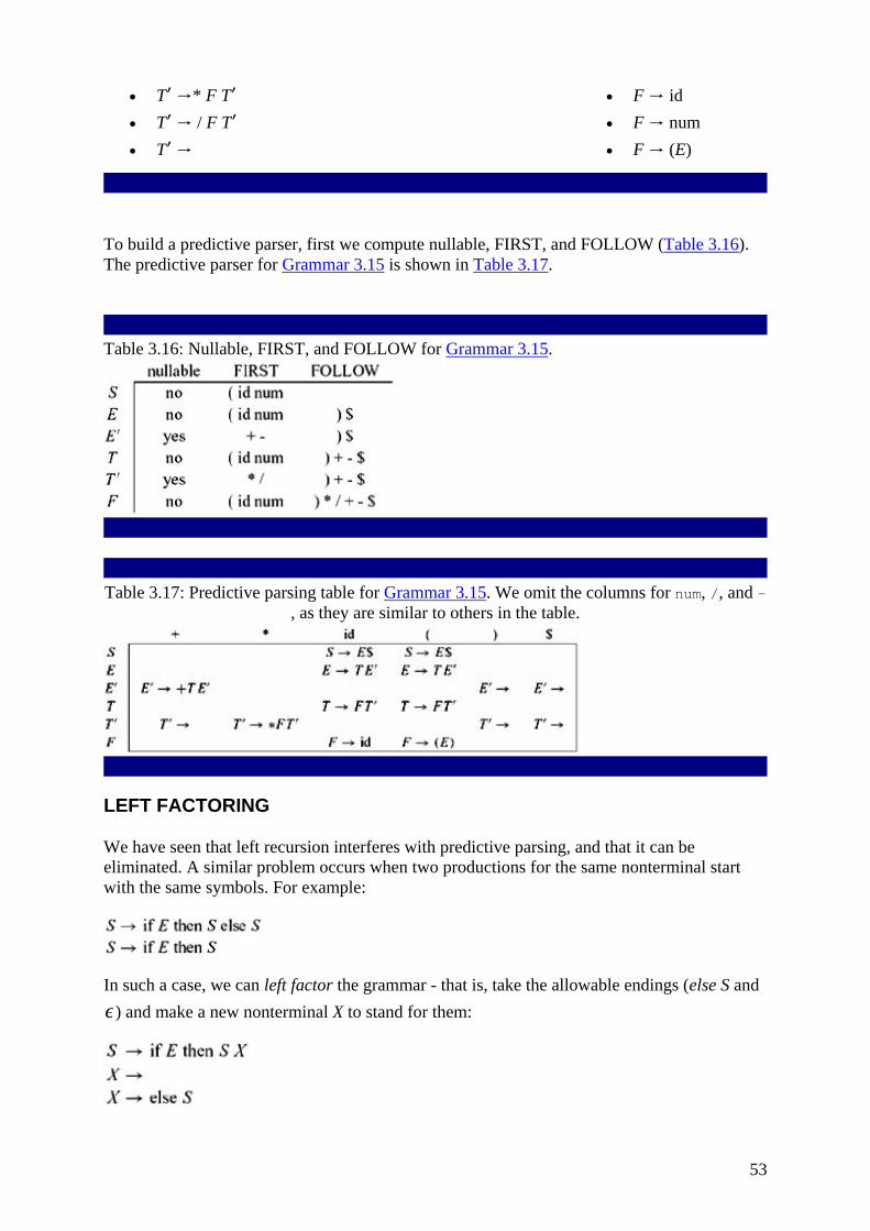
53

• T′ →* F T′ • T′ → / F T′ • T′ →

• F → id • F → num • F → (E)

To build a predictive parser, first we compute nullable, FIRST, and FOLLOW (Table 3.16). The predictive parser for Grammar 3.15 is shown in Table 3.17.

Table 3.16: Nullable, FIRST, and FOLLOW for Grammar 3.15.

Table 3.17: Predictive parsing table for Grammar 3.15. We omit the columns for num, /, and -

, as they are similar to others in the table.

LEFT FACTORING

We have seen that left recursion interferes with predictive parsing, and that it can be eliminated. A similar problem occurs when two productions for the same nonterminal start with the same symbols. For example:

In such a case, we can left factor the grammar - that is, take the allowable endings (else S and ∊) and make a new nonterminal X to stand for them:

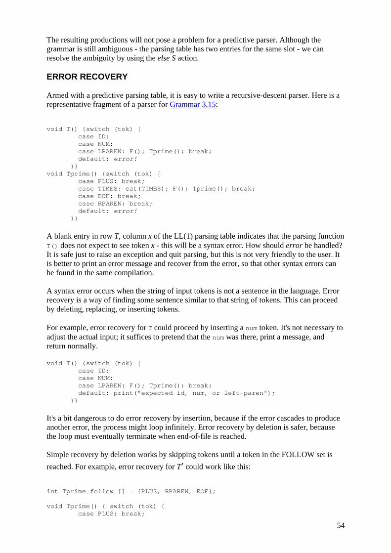
54

The resulting productions will not pose a problem for a predictive parser. Although the grammar is still ambiguous - the parsing table has two entries for the same slot - we can resolve the ambiguity by using the else S action.

ERROR RECOVERY

Armed with a predictive parsing table, it is easy to write a recursive-descent parser. Here is a representative fragment of a parser for Grammar 3.15:

void T() {switch (tok) { case ID: case NUM: case LPAREN: F(); Tprime(); break; default: error! }} void Tprime() {switch (tok) { case PLUS: break; case TIMES: eat(TIMES); F(); Tprime(); break; case EOF: break; case RPAREN: break; default: error! }}

A blank entry in row T, column x of the LL(1) parsing table indicates that the parsing function T() does not expect to see token x - this will be a syntax error. How should error be handled? It is safe just to raise an exception and quit parsing, but this is not very friendly to the user. It is better to print an error message and recover from the error, so that other syntax errors can be found in the same compilation.

A syntax error occurs when the string of input tokens is not a sentence in the language. Error recovery is a way of finding some sentence similar to that string of tokens. This can proceed by deleting, replacing, or inserting tokens.

For example, error recovery for T could proceed by inserting a num token. It's not necessary to adjust the actual input; it suffices to pretend that the num was there, print a message, and return normally.

void T() {switch (tok) { case ID: case NUM: case LPAREN: F(); Tprime(); break; default: print("expected id, num, or left-paren"); }}

It's a bit dangerous to do error recovery by insertion, because if the error cascades to produce another error, the process might loop infinitely. Error recovery by deletion is safer, because the loop must eventually terminate when end-of-file is reached.

Simple recovery by deletion works by skipping tokens until a token in the FOLLOW set is reached. For example, error recovery for T′ could work like this:

int Tprime_follow [] = {PLUS, RPAREN, EOF}; void Tprime() { switch (tok) { case PLUS: break;

55

case TIMES: eat(TIMES); F(); Tprime(); break; case RPAREN: break; case EOF: break; default: print("expected +, *, right-paren, or end-of-file"); skipto(Tprime_follow); }}

A recursive-descent parser's error-recovery mechanisms must be adjusted (sometimes by trial and error) to avoid a long cascade of error-repair messages resulting from a single token out of place.

3.3 LR PARSING

The weakness of LL(k) parsing techniques is that they must predict which production to use, having seen only the first k tokens of the right-hand side. A more powerful technique, LR(k) parsing, is able to postpone the decision until it has seen input tokens corresponding to the entire right-hand side of the production in question (and k more input tokens beyond).

LR(k) stands for left-to-right parse, rightmost-derivation, k-token lookahead. The use of a rightmost derivation seems odd; how is that compatible with a left-to-right parse? Figure 3.18 illustrates an LR parse of the program

a:=7; b:=c+(d:=5+6,d)

56

Figure 3.18: Shift-reduce parse of a sentence. Numeric subscripts in the Stack are DFA state numbers; see Table 3.19.

using Grammar 3.1, augmented with a new start production S′ → S$.

The parser has a stack and an input. The first k tokens of the input are the lookahead. Based on the contents of the stack and the lookahead, the parser performs two kinds of actions:

Shift: Move the first input token to the top of the stack.

Reduce: Choose a grammar rule X → A B C; pop C, B, A from the top of the stack; push X onto the stack.

Initially, the stack is empty and the parser is at the beginning of the input. The action of shifting the end-of-file marker $ is called accepting and causes the parser to stop successfully.

In Figure 3.18, the stack and input are shown after every step, along with an indication of which action has just been performed. The concatenation of stack and input is always one line of a rightmost derivation; in fact, Figure 3.18 shows the rightmost derivation of the input string, upside-down.

57

LR PARSING ENGINE

How does the LR parser know when to shift and when to reduce? By using a deterministic finite automaton! The DFA is not applied to the input - finite automata are too weak to parse context-free grammars - but to the stack. The edges of the DFA are labeled by the symbols (terminals and nonterminals) that can appear on the stack. Table 3.19 is the transition table for Grammar 3.1.

Table 3.19: LR parsing table for Grammar 3.1.

The elements in the transition table are labeled with four kinds of actions:

sn Shift into state n; gn Goto state n; rk Reduce by rule k; a Accept;

Error (denoted by a blank entry in the table).

To use this table in parsing, treat the shift and goto actions as edges of a DFA, and scan the stack. For example, if the stack is id := E, then the DFA goes from state 1 to 4 to 6 to 11. If the next input token is a semicolon, then the ";" column in state 11 says to reduce by rule 2. The second rule of the grammar is S → id:=E, so the top three tokens are popped from the stack and S is pushed.

58

The action for "+" in state 11 is to shift; so if the next token had been + instead, it would have been eaten from the input and pushed on the stack.

Rather than rescan the stack for each token, the parser can remember instead the state reached for each stack element. Then the parsing algorithm is

Look up top stack state, and input symbol, to get action; If action is

Shift(n): Advance input one token; push n on stack. Reduce(k): Pop stack as many times as the number of symbols on the right-hand side of rule

k; Let X be the left-hand-side symbol of rule k;

In the state now on top of stack, look up X to get "goto n"; Push n on top of stack.

Accept: Stop parsing, report success. Error: Stop parsing, report failure.

LR(0) PARSER GENERATION

An LR(k) parser uses the contents of its stack and the next k tokens of the input to decide which action to take. Table 3.19 shows the use of one symbol of lookahead. For k = 2, the table has columns for every two-token sequence and so on; in practice, k > 1 is not used for compilation. This is partly because the tables would be huge, but more because most reasonable programming languages can be described by LR(1) grammars.

LR(0) grammars are those that can be parsed looking only at the stack, making shift/reduce decisions without any lookahead. Though this class of grammars is too weak to be very useful, the algorithm for constructing LR(0) parsing tables is a good introduction to the LR(1) parser construction algorithm.

We will use Grammar 3.20 to illustrate LR(0) parser generation. Consider what the parser for this grammar will be doing. Initially, it will have an empty stack, and the input will be a complete S-sentence followed by $; that is, the right-hand side of the S′ rule will be on the input. We indicate this as S′ → .S$ where the dot indicates the current position of the parser.

GRAMMAR 3.20

0. S′ → S$

1. S → (L) 2. S → x

3. L → S 4. L → L, S

In this state, where the input begins with S, that means that it begins with any possible right-hand side of an S-production; we indicate that by

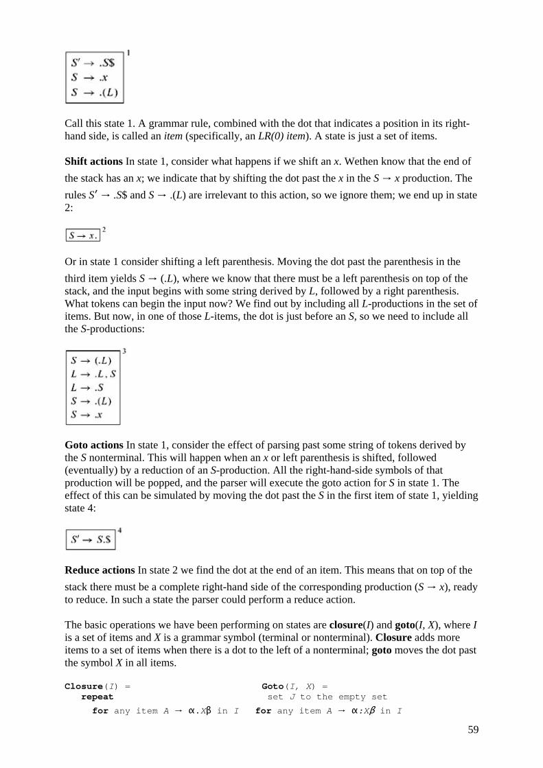
59

Call this state 1. A grammar rule, combined with the dot that indicates a position in its right-hand side, is called an item (specifically, an LR(0) item). A state is just a set of items.

Shift actions In state 1, consider what happens if we shift an x. Wethen know that the end of the stack has an x; we indicate that by shifting the dot past the x in the S → x production. The rules S′ → .S$ and S → .(L) are irrelevant to this action, so we ignore them; we end up in state 2:

Or in state 1 consider shifting a left parenthesis. Moving the dot past the parenthesis in the third item yields S → (.L), where we know that there must be a left parenthesis on top of the stack, and the input begins with some string derived by L, followed by a right parenthesis. What tokens can begin the input now? We find out by including all L-productions in the set of items. But now, in one of those L-items, the dot is just before an S, so we need to include all the S-productions:

Goto actions In state 1, consider the effect of parsing past some string of tokens derived by the S nonterminal. This will happen when an x or left parenthesis is shifted, followed (eventually) by a reduction of an S-production. All the right-hand-side symbols of that production will be popped, and the parser will execute the goto action for S in state 1. The effect of this can be simulated by moving the dot past the S in the first item of state 1, yielding state 4:

Reduce actions In state 2 we find the dot at the end of an item. This means that on top of the stack there must be a complete right-hand side of the corresponding production (S → x), ready to reduce. In such a state the parser could perform a reduce action.

The basic operations we have been performing on states are closure(I) and goto(I, X), where I is a set of items and X is a grammar symbol (terminal or nonterminal). Closure adds more items to a set of items when there is a dot to the left of a nonterminal; goto moves the dot past the symbol X in all items.

Closure(I) = Goto(I, X) = repeat set J to the empty set

for any item A → α.Xβ in I for any item A → α:Xβ in I

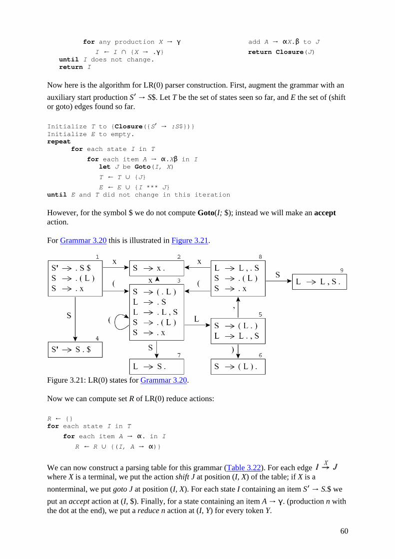
60

for any production X → γ add A → αX.β to J I ← I ∩ {X → .γ} return Closure(J) until I does not change. return I

Now here is the algorithm for LR(0) parser construction. First, augment the grammar with an auxiliary start production S′ → S$. Let T be the set of states seen so far, and E the set of (shift or goto) edges found so far.

Initialize T to {Closure({S′ → :S$})} Initialize E to empty. repeat for each state I in T

for each item A → α.Xβ in I let J be Goto(I, X)

T ← T ∪ {J} E ← E ∪ {I *** J} until E and T did not change in this iteration

However, for the symbol $ we do not compute Goto(I; $); instead we will make an accept action.

For Grammar 3.20 this is illustrated in Figure 3.21.

Figure 3.21: LR(0) states for Grammar 3.20.

Now we can compute set R of LR(0) reduce actions:

R ← {} for each state I in T

for each item A → α. in I R ← R ∪ {(I, A → α)}

We can now construct a parsing table for this grammar (Table 3.22). For each edge where X is a terminal, we put the action shift J at position (I, X) of the table; if X is a nonterminal, we put goto J at position (I, X). For each state I containing an item S′ → S.$ we put an accept action at (I, $). Finally, for a state containing an item A → γ. (production n with the dot at the end), we put a reduce n action at (I, Y) for every token Y.

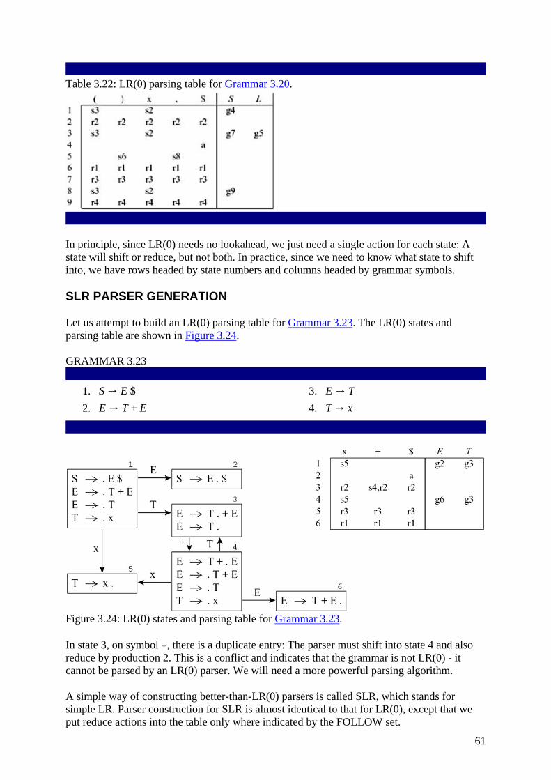
61

Table 3.22: LR(0) parsing table for Grammar 3.20.

In principle, since LR(0) needs no lookahead, we just need a single action for each state: A state will shift or reduce, but not both. In practice, since we need to know what state to shift into, we have rows headed by state numbers and columns headed by grammar symbols.

SLR PARSER GENERATION

Let us attempt to build an LR(0) parsing table for Grammar 3.23. The LR(0) states and parsing table are shown in Figure 3.24.

GRAMMAR 3.23

1. S → E $ 2. E → T + E

3. E → T 4. T → x

Figure 3.24: LR(0) states and parsing table for Grammar 3.23.

In state 3, on symbol +, there is a duplicate entry: The parser must shift into state 4 and also reduce by production 2. This is a conflict and indicates that the grammar is not LR(0) - it cannot be parsed by an LR(0) parser. We will need a more powerful parsing algorithm.

A simple way of constructing better-than-LR(0) parsers is called SLR, which stands for simple LR. Parser construction for SLR is almost identical to that for LR(0), except that we put reduce actions into the table only where indicated by the FOLLOW set.

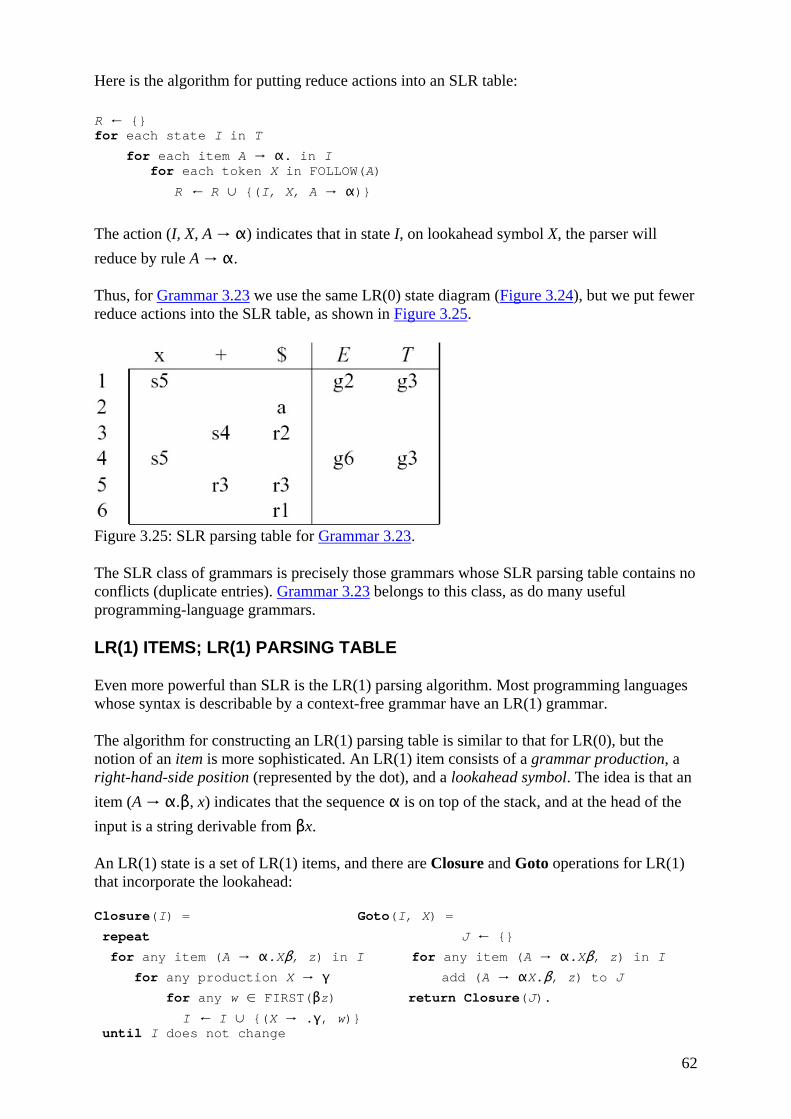
62

Here is the algorithm for putting reduce actions into an SLR table:


for each item A → α. in I for each token X in FOLLOW(A)

R ← R ∪ {(I, X, A → α)}

The action (I, X, A → α) indicates that in state I, on lookahead symbol X, the parser will reduce by rule A → α.

Thus, for Grammar 3.23 we use the same LR(0) state diagram (Figure 3.24), but we put fewer reduce actions into the SLR table, as shown in Figure 3.25.

Figure 3.25: SLR parsing table for Grammar 3.23.

The SLR class of grammars is precisely those grammars whose SLR parsing table contains no conflicts (duplicate entries). Grammar 3.23 belongs to this class, as do many useful programming-language grammars.

LR(1) ITEMS; LR(1) PARSING TABLE

Even more powerful than SLR is the LR(1) parsing algorithm. Most programming languages whose syntax is describable by a context-free grammar have an LR(1) grammar.

The algorithm for constructing an LR(1) parsing table is similar to that for LR(0), but the notion of an item is more sophisticated. An LR(1) item consists of a grammar production, a right-hand-side position (represented by the dot), and a lookahead symbol. The idea is that an item (A → α.β, x) indicates that the sequence α is on top of the stack, and at the head of the input is a string derivable from βx.

An LR(1) state is a set of LR(1) items, and there are Closure and Goto operations for LR(1) that incorporate the lookahead:

Closure(I) = Goto(I, X) =

repeat J ← {} for any item (A → α.Xβ, z) in I for any item (A → α.Xβ, z) in I for any production X → γ add (A → αX.β, z) to J for any w ∈ FIRST(βz) return Closure(J). I ← I ∪ {(X → .γ, w)} until I does not change

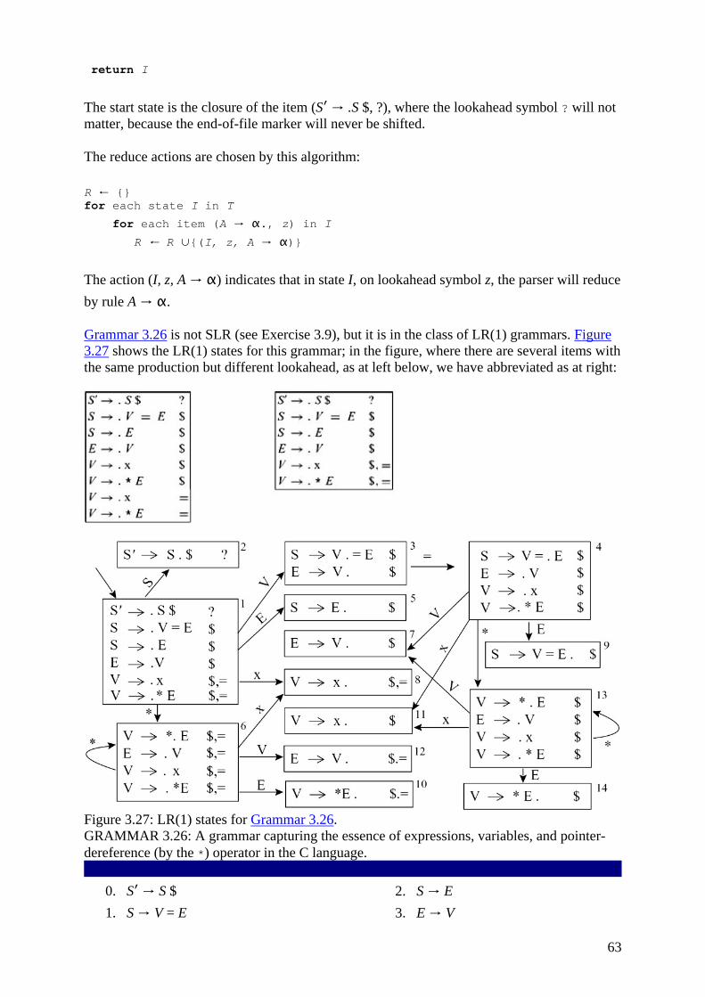
63

return I

The start state is the closure of the item (S′ → .S $, ?), where the lookahead symbol ? will not matter, because the end-of-file marker will never be shifted.

The reduce actions are chosen by this algorithm:


for each item (A → α., z) in I R ← R ∪{(I, z, A → α)}

The action (I, z, A → α) indicates that in state I, on lookahead symbol z, the parser will reduce by rule A → α.

Grammar 3.26 is not SLR (see Exercise 3.9), but it is in the class of LR(1) grammars. Figure 3.27 shows the LR(1) states for this grammar; in the figure, where there are several items with the same production but different lookahead, as at left below, we have abbreviated as at right:

Figure 3.27: LR(1) states for Grammar 3.26. GRAMMAR 3.26: A grammar capturing the essence of expressions, variables, and pointer-dereference (by the *) operator in the C language.

0. S′ → S $ 1. S → V = E

2. S → E 3. E → V

64

4. V → x 5. V → * E

The LR(1) parsing table derived from this state graph is Table 3.28a. Wherever the dot is at the end of a production (as in state 3 of Figure 3.27, where it is at the end of production E → V ), then there is a reduce action for that production in the LR(1) table, in the row corresponding to the state number and the column corresponding to the lookahead of the item (in this case, the lookahead is $). Whenever the dot is to the left of a terminal symbol or nonterminal, there is a corresponding shift or goto action in the LR(1) parsing table, just as there would be in an LR(0) table.

Table 3.28: LR(1) and LALR(1) parsing tables for Grammar 3.26.

LALR(1) PARSING TABLES

LR(1) parsing tables can be very large, with many states. A smaller table can be made by merging any two states whose items are identical except for lookahead sets. The result parser is called an LALR(1) parser, for lookahead LR(1).

For example, the items in states 6 and 13 of the LR(1) parser for Grammar 3.26 (Figure 3.27) are identical if the lookahead sets are ignored. Also, states 7 and 12 are identical except for lookahead, as are states 8 and 11 and states 10 and 14. Merging these pairs of states gives the LALR(1) parsing table shown in Table 3.28b.

For some grammars, the LALR(1) table contains reduce-reduce conflicts where the LR(1) table has none, but in practice the difference matters little. What does matter is that the LALR(1) parsing table requires less memory to represent than the LR(1) table, since there can be many fewer states.

65

HIERARCHY OF GRAMMAR CLASSES

A grammar is said to be LALR(1) if its LALR(1) parsing table contains no conflicts. All SLR grammars are LALR(1), but not vice versa. Figure 3.29 shows the relationship between several classes of grammars.

Figure 3.29: A hierarchy of grammar classes.

Any reasonable programming language has a LALR(1) grammar, and there are many parser-generator tools available for LALR(1) grammars. For this reason, LALR(1) has become a standard for programming languages and for automatic parser generators.

LR PARSING OF AMBIGUOUS GRAMMARS

Many programming languages have grammar rules such as

• S → if E then S else S • S → if E then S • S → other

which allow programs such as

if a then if b then s1 else s2

Such a program could be understood in two ways:

(1) if a then { if b then s1 else s2 } (2) if a then { if b then s1 } else s2

In most programming languages, an else must match the most recent possible then, so interpretation (1) is correct. In the LR parsing table there will be a shift-reduce conflict:

66

Shifting corresponds to interpretation (1) and reducing to interpretation (2).

The ambiguity can be eliminated by introducing auxiliary nonterminals M (for matched statement)and U (for unmatched statement):

• S → M • S → U • M → if E then M else M • M → other • U → if E then S • U → if E then M else U

But instead of rewriting the grammar, we can leave the grammar unchanged and tolerate the shift-reduce conflict. In constructing the parsing table this conflict should be resolved by shifting, since we prefer interpretation (1).

It is often possible to use ambiguous grammars by resolving shift-reduce conflicts in favor of shifting or reducing, as appropriate. But it is best to use this technique sparingly, and only in cases (such as the dangling-else described here, and operator-precedence to be described on page 74) that are well understood. Most shift-reduce conflicts, and probably all reduce-reduce conflicts, should not be resolved by fiddling with the parsing table. They are symptoms of an ill-specified grammar, and they should be resolved by eliminating ambiguities.

3.4 USING PARSER GENERATORS

The task of constructing a parser is simple enough to be automated. In the previous chapter we described the lexical-analyzer aspects of JavaCC and SableCC. Here we will discuss the parser-generator aspects of these tools. Documentation for JavaCC and SableCC are available via this book's Web site.

JAVACC

JavaCC is an LL(k) parser generator. Productions are of the form:

void Assignment() : {} { Identifier() "=" Expression() ";" }

where the left-hand side is Assignment(); the right-hand side is enclosed between the last two curly brackets; Assignment(), Identifier(), and Expression() are nonterminal symbols; and "=" and ";" are terminal symbols.

Grammar 3.30 can be represented as a JavaCC grammar as shown in Grammar 3.31. Notice that if we had written the production for StmList() in the style of Grammar 3.30, that is,

void StmList() : {} { Stm() | StmList( ) ";" Stm() }

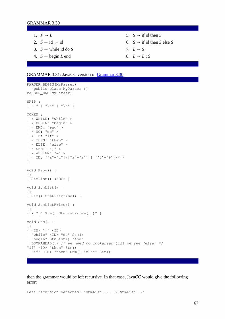
67

GRAMMAR 3.30

1. P → L 2. S → id := id 3. S → while id do S 4. S → begin L end

5. S → if id then S 6. S → if id then S else S 7. L → S 8. L → L ; S

GRAMMAR 3.31: JavaCC version of Grammar 3.30. PARSER_BEGIN(MyParser) public class MyParser {} PARSER_END(MyParser) SKIP : { " " | "\t" | "\n" } TOKEN : { < WHILE: "while" > | < BEGIN: "begin" > | < END: "end" > | < DO: "do" > | < IF: "if" > | < THEN: "then" > | < ELSE: "else" > | < SEMI: ";" > | < ASSIGN: "=" > | < ID: ["a"-"z"](["a"-"z"] | ["0"-"9"])* > } void Prog() : {} { StmList() <EOF> } void StmList() : {} { Stm() StmListPrime() } void StmListPrime() : {} { ( ";" Stm() StmListPrime() )? } void Stm() : {} { <ID> "=" <ID> | "while" <ID> "do" Stm() | "begin" StmList() "end" | LOOKAHEAD(5) /* we need to lookahead till we see "else" */ "if" <ID> "then" Stm() | "if" <ID> "then" Stm() "else" Stm() }

then the grammar would be left recursive. In that case, JavaCC would give the following error:

Left recursion detected: "StmList... --> StmList..."

68

We used the techniques mentioned earlier to remove the left recursion and arrive at Grammar 3.31.

SABLECC

SableCC is an LALR(1) parser generator. Productions are of the form:

assignment = identifier assign expression semicolon ;

where the left-hand side is assignment; the right-hand side is enclosed between = and ;; assignment, identifier, and expression are nonterminal symbols; and assign and semicolon are terminal symbols that are defined in an earlier part of the syntax specification.

Grammar 3.30 can be represented as a SableCC grammar as shown in Grammar 3.32. When there is more than one alternative, SableCC requires a name for each alternative. A name is given to an alternative in the grammar by prefixing the alternative with an identifier between curly brackets. Also, if the same grammar symbol appears twice in the same alternative of a production, SableCC requires a name for at least one of the two elements. Element names are specified by prefixing the element with an identifier between square brackets followed by a colon.

GRAMMAR 3.32: SableCC version of Grammar 3.30. Tokens while = 'while'; begin = 'begin'; end = 'end'; do = 'do'; if = 'if'; then = 'then'; else = 'else'; semi = ';'; assign = '='; whitespace = (' ' | '\t' | '\n')+; id = ['a'..'z'](['a'..'z'] | ['0'..'9'])*; Ignored Tokens whitespace; Productions prog = stmlist; stm = {assign} [left]:id assign [right]:id | {while} while id do stm | {begin} begin stmlist end | {if_then} if id then stm | {if_then_else} if id then [true_stm]:stm else [false_stm]:stm; stmlist = {stmt} stm | {stmtlist} stmlist semi stm;

SableCC reports shift-reduce and reduce-reduce conflicts. A shift-reduce conflict is a choice between shifting and reducing; a reduce-reduce conflict is a choice of reducing by two different rules.

SableCC will report that the Grammar 3.32 has a shift-reduce conflict. The conflict can be examined by reading the detailed error message SableCC produces, as shown in Figure 3.33.

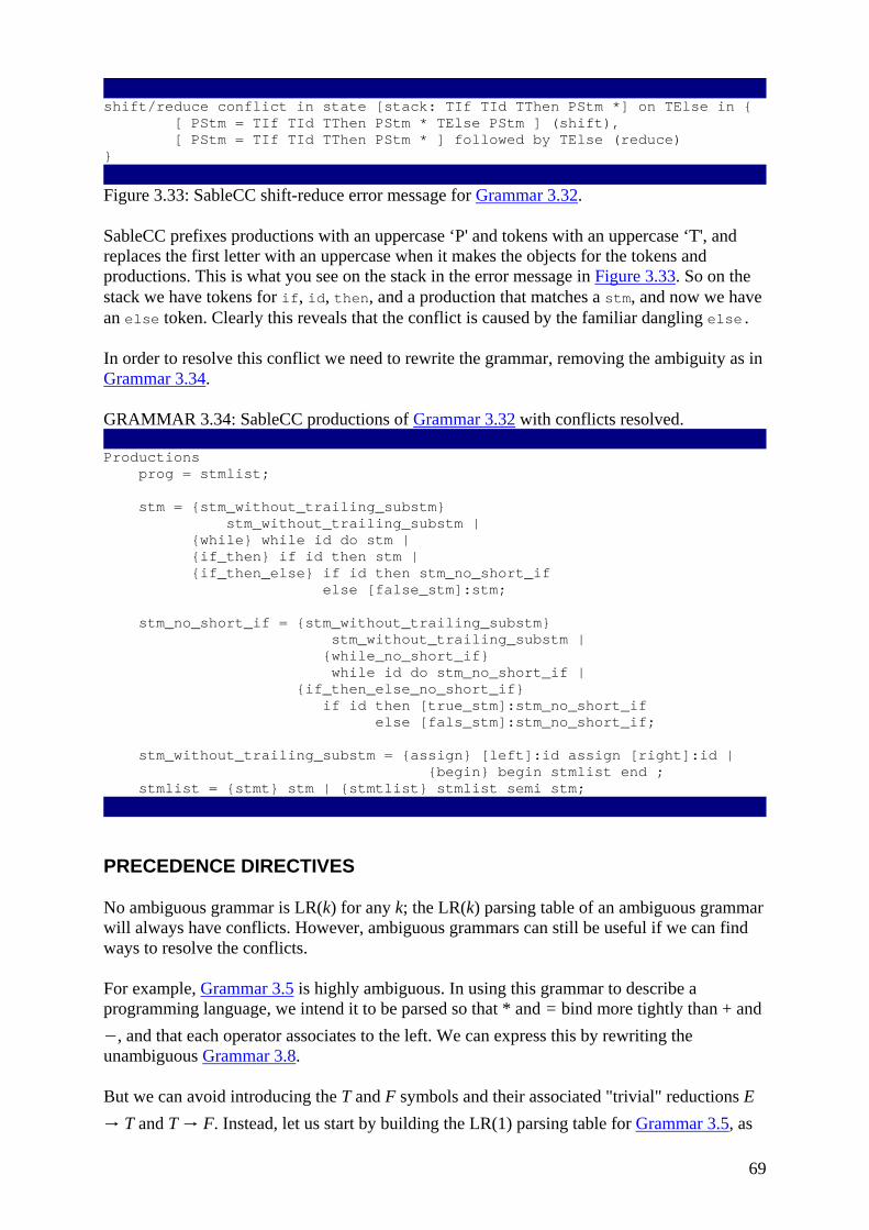
69

shift/reduce conflict in state [stack: TIf TId TThen PStm *] on TElse in { [ PStm = TIf TId TThen PStm * TElse PStm ] (shift), [ PStm = TIf TId TThen PStm * ] followed by TElse (reduce) }

Figure 3.33: SableCC shift-reduce error message for Grammar 3.32.

SableCC prefixes productions with an uppercase ‘P' and tokens with an uppercase ‘T', and replaces the first letter with an uppercase when it makes the objects for the tokens and productions. This is what you see on the stack in the error message in Figure 3.33. So on the stack we have tokens for if, id, then, and a production that matches a stm, and now we have an else token. Clearly this reveals that the conflict is caused by the familiar dangling else.

In order to resolve this conflict we need to rewrite the grammar, removing the ambiguity as in Grammar 3.34.

GRAMMAR 3.34: SableCC productions of Grammar 3.32 with conflicts resolved. Productions prog = stmlist; stm = {stm_without_trailing_substm} stm_without_trailing_substm | {while} while id do stm | {if_then} if id then stm | {if_then_else} if id then stm_no_short_if else [false_stm]:stm; stm_no_short_if = {stm_without_trailing_substm} stm_without_trailing_substm | {while_no_short_if} while id do stm_no_short_if | {if_then_else_no_short_if} if id then [true_stm]:stm_no_short_if else [fals_stm]:stm_no_short_if; stm_without_trailing_substm = {assign} [left]:id assign [right]:id | {begin} begin stmlist end ; stmlist = {stmt} stm | {stmtlist} stmlist semi stm;

PRECEDENCE DIRECTIVES

No ambiguous grammar is LR(k) for any k; the LR(k) parsing table of an ambiguous grammar will always have conflicts. However, ambiguous grammars can still be useful if we can find ways to resolve the conflicts.

For example, Grammar 3.5 is highly ambiguous. In using this grammar to describe a programming language, we intend it to be parsed so that * and = bind more tightly than + and −, and that each operator associates to the left. We can express this by rewriting the unambiguous Grammar 3.8.

But we can avoid introducing the T and F symbols and their associated "trivial" reductions E → T and T → F. Instead, let us start by building the LR(1) parsing table for Grammar 3.5, as

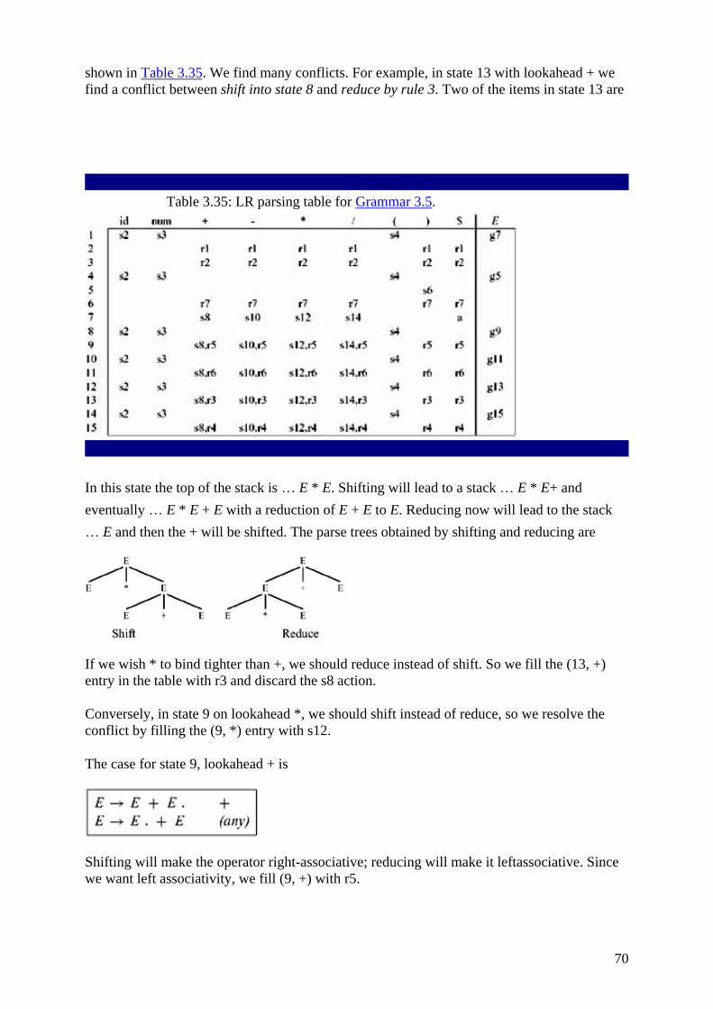
70

shown in Table 3.35. We find many conflicts. For example, in state 13 with lookahead + we find a conflict between shift into state 8 and reduce by rule 3. Two of the items in state 13 are

Table 3.35: LR parsing table for Grammar 3.5.

In this state the top of the stack is … E * E. Shifting will lead to a stack … E * E+ and eventually … E * E + E with a reduction of E + E to E. Reducing now will lead to the stack … E and then the + will be shifted. The parse trees obtained by shifting and reducing are

If we wish * to bind tighter than +, we should reduce instead of shift. So we fill the (13, +) entry in the table with r3 and discard the s8 action.

Conversely, in state 9 on lookahead *, we should shift instead of reduce, so we resolve the conflict by filling the (9, *) entry with s12.

The case for state 9, lookahead + is

Shifting will make the operator right-associative; reducing will make it leftassociative. Since we want left associativity, we fill (9, +) with r5.

71

Consider the expression a − b − c. In most programming languages, this associates to the left, as if written (a − b) − c. But suppose we believe that this expression is inherently confusing, and we want to force the programmer to put in explicit parentheses, either (a − b) − c or a − (b − c). Then we say that the minus operator is nonassociative, and we would fill the (11, −) entry with an error entry.

The result of all these decisions is a parsing table with all conflicts resolved (Table 3.36).

Table 3.36: Conflicts of Table 3.35 resolved.

Yacc has precedence directives to indicate the resolution of this class of shift-reduce conflicts. (Unfortunately, SableCC does not have precedence directives.) A series of declarations such as

precedence nonassoc EQ, NEQ; precedence left PLUS, MINUS; precedence left TIMES, DIV; precedence right EXP;

indicates that + and - are left-associative and bind equally tightly; that * and / are left-associative and bind more tightly than +; that ⁁ is right-associative and binds most tightly; and that = and ≠ are nonassociative, and bind more weakly than +.

In examining a shift-reduce conflict such as

there is the choice of shifting a token and reducing by a rule. Should the rule or the token be given higher priority? The precedence declarations (precedence left, etc.) give priorities to the tokens; the priority of a rule is given by the last token occurring on the right-hand side of that rule. Thus the choice here is between a rule with priority * and a token with priority +; the rule has higher priority, so the conflict is resolved in favor of reducing.

When the rule and token have equal priority, then a left precedence favors reducing, right favors shifting, and nonassoc yields an error action.

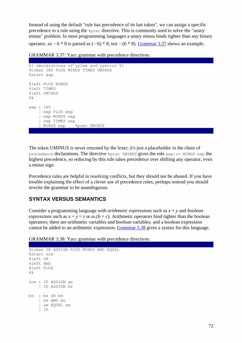
72

Instead of using the default "rule has precedence of its last token", we can assign a specific precedence to a rule using the %prec directive. This is commonly used to solve the "unary minus" problem. In most programming languages a unary minus binds tighter than any binary operator, so −6 * 8 is parsed as (−6) * 8, not −(6 * 8). Grammar 3.37 shows an example.

GRAMMAR 3.37: Yacc grammar with precedence directives. %{ declarations of yylex and yyerror %} %token INT PLUS MINUS TIMES UMINUS %start exp %left PLUS MINUS %left TIMES %left UMINUS %% exp : INT | exp PLUS exp | exp MINUS exp | exp TIMES exp | MINUS exp %prec UMINUS

The token UMINUS is never returned by the lexer; it's just a placeholder in the chain of precedence declarations. The directive %prec UMINUS gives the rule exp::= MINUS exp the highest precedence, so reducing by this rule takes precedence over shifting any operator, even a minus sign.

Precedence rules are helpful in resolving conflicts, but they should not be abused. If you have trouble explaining the effect of a clever use of precedence rules, perhaps instead you should rewrite the grammar to be unambiguous.

SYNTAX VERSUS SEMANTICS

Consider a programming language with arithmetic expressions such as x + y and boolean expressions such as x + y = z or a&(b = c). Arithmetic operators bind tighter than the boolean operators; there are arithmetic variables and boolean variables; and a boolean expression cannot be added to an arithmetic expression. Grammar 3.38 gives a syntax for this language.

GRAMMAR 3.38: Yacc grammar with precedence directives. %token ID ASSIGN PLUS MINUS AND EQUAL %start stm %left OR %left AND %left PLUS %% stm : ID ASSIGN ae | ID ASSIGN be be : be OR be | be AND be | ae EQUAL ae | ID

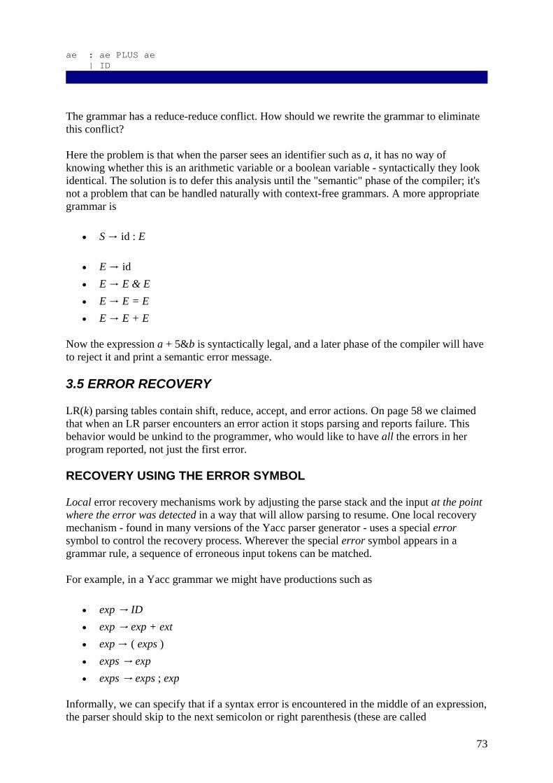
73

ae : ae PLUS ae | ID

The grammar has a reduce-reduce conflict. How should we rewrite the grammar to eliminate this conflict?

Here the problem is that when the parser sees an identifier such as a, it has no way of knowing whether this is an arithmetic variable or a boolean variable - syntactically they look identical. The solution is to defer this analysis until the "semantic" phase of the compiler; it's not a problem that can be handled naturally with context-free grammars. A more appropriate grammar is

• S → id : E

• E → id • E → E & E • E → E = E • E → E + E

Now the expression a + 5&b is syntactically legal, and a later phase of the compiler will have to reject it and print a semantic error message.

3.5 ERROR RECOVERY

LR(k) parsing tables contain shift, reduce, accept, and error actions. On page 58 we claimed that when an LR parser encounters an error action it stops parsing and reports failure. This behavior would be unkind to the programmer, who would like to have all the errors in her program reported, not just the first error.

RECOVERY USING THE ERROR SYMBOL

Local error recovery mechanisms work by adjusting the parse stack and the input at the point where the error was detected in a way that will allow parsing to resume. One local recovery mechanism - found in many versions of the Yacc parser generator - uses a special error symbol to control the recovery process. Wherever the special error symbol appears in a grammar rule, a sequence of erroneous input tokens can be matched.

For example, in a Yacc grammar we might have productions such as

• exp → ID • exp → exp + ext • exp → ( exps ) • exps → exp • exps → exps ; exp

Informally, we can specify that if a syntax error is encountered in the middle of an expression, the parser should skip to the next semicolon or right parenthesis (these are called

74

synchronizing tokens) and resume parsing. We do this by adding error-recovery productions such as

• exp → ( error ) • exps → error ; exp

What does the parser generator do with the error symbol? In parser generation, error is considered a terminal symbol, and shift actions are entered in the parsing table for it as if it were an ordinary token.

When the LR parser reaches an error state, it takes the following actions:

1. Pop the stack (if necessary) until a state is reached in which the action for the error token is shift.

2. Shift the error token. 3. Discard input symbols (if necessary) until a lookahead is reached that has a nonerror

action in the current state. 4. Resume normal parsing.

In the two error productions illustrated above, we have taken care to follow the error symbol with an appropriate synchronizing token - in this case, a right parenthesis or semicolon. Thus, the "nonerror action" taken in step 3 will always shift. If instead we used the production exp → error, the "nonerror action" would be reduce, and (in an SLR or LALR parser) it is possible that the original (erroneous) lookahead symbol would cause another error after the reduce action, without having advanced the input. Therefore, grammar rules that contain error not followed by a token should be used only when there is no good alternative.

Caution One can attach semantic actions to Yacc grammar rules; whenever a rule is reduced, its semantic action is executed. Chapter 4 explains the use of semantic actions. Popping states from the stack can lead to seemingly "impossible" semantic actions, especially if the actions contain side effects. Consider this grammar fragment:

statements: statements exp SEMICOLON | statements error SEMICOLON | /* empty */ exp : increment exp decrement |ID increment: LPAREN {: nest=nest+1; :} decrement: RPAREN {: nest=nest-1; :}

"Obviously" it is true that whenever a semicolon is reached, the value of nest is zero, because it is incremented and decremented in a balanced way according to the grammar of expressions. But if a syntax error is found after some left parentheses have been parsed, then states will be popped from the stack without "completing" them, leading to a nonzero value of nest. The best solution to this problem is to have side-effect-free semantic actions that build abstract syntax trees, as described in Chapter 4.

Unfortunately, neither JavaCC nor SableCC support the error-symbol errorrecovery method, nor the kind of global error repair described below.

75

GLOBAL ERROR REPAIR

Global error repair finds the smallest set of insertions and deletions that would turn the source string into a syntactically correct string, even if the insertions and deletions are not at a point where an LL or LR parser would first report an error.

Burke-Fisher error repair We will describe a limited but useful form of global error repair, which tries every possible single-token insertion, deletion, or replacement at every point that occurs no earlier than K tokens before the point where the parser reported the error. Thus, with K = 15, if the parsing engine gets stuck at the 100th token of the input, then it will try every possible repair between the 85th and 100th tokens.

The correction that allows the parser to parse furthest past the original reported error is taken as the best error repair. Thus, if a single-token substitution of var for type at the 98th token allows the parsing engine to proceed past the 104th token without getting stuck, this repair is a successful one. Generally, if a repair carries the parser R = 4 tokens beyond where it originally got stuck, this is "good enough."

The advantage of this technique is that the LL(k) or LR(k) (or LALR, etc.) grammar is not modified at all (no error productions), nor are the parsing tables modified. Only the parsing engine, which interprets the parsing tables, is modified.

The parsing engine must be able to back up K tokens and reparse. To do this, it needs to remember what the parse stack looked like K tokens ago. Therefore, the algorithm maintains two parse stacks: the current stack and the old stack. A queue of K tokens is kept; as each new token is shifted, it is pushed on the current stack and also put onto the tail of the queue; simultaneously, the head of the queue is removed and shifted onto the old stack. With each shift onto the old or current stack, the appropriate reduce actions are also performed. Figure 3.39 illustrates the two stacks and queue.

Figure 3.39: Burke-Fisher parsing, with an error-repair queue. Figure 3.18 shows the complete parse of this string according to Table 3.19.

Now suppose a syntax error is detected at the current token. For each possible insertion, deletion, or substitution of a token at any position of the queue, the Burke-Fisher error repairer makes that change to within (a copy of) the queue, then attempts to reparse from the old stack. The success of a modification is in how many tokens past the current token can be parsed; generally, if three or four new tokens can be parsed, this is considered a completely successful repair.

76

In a language with N kinds of tokens, there are K + K · N + K · N possible deletions, insertions, and substitutions within the K -token window. Trying this many repairs is not very costly, especially considering that it happens only when a syntax error is discovered, not during ordinary parsing.

Semantic actions Shift and reduce actions are tried repeatedly and discarded during the search for the best error repair. Parser generators usually perform programmer-specified semantic actions along with each reduce action, but the programmer does not expect that these actions will be performed repeatedly and discarded - they may have side effects. Therefore, a Burke-Fisher parser does not execute any of the semantic actions as reductions are performed on the current stack, but waits until the same reductions are performed (permanently) on the old stack.

This means that the lexical analyzer may be up to K + R tokens ahead of the point to which semantic actions have been performed. If semantic actions affect lexical analysis - as they do in C, compiling the typedef feature - this can be a problem with the Burke-Fisher approach. For languages with a pure context-free grammar approach to syntax, the delay of semantic actions poses no problem.

Semantic values for insertions In repairing an error by insertion, the parser needs to provide a semantic value for each token it inserts, so that semantic actions can be performed as if the token had come from the lexical analyzer. For punctuation tokens no value is necessary, but when tokens such as numbers or identifiers must be inserted, where can the value come from? The ML-Yacc parser generator, which uses Burke-Fischer error correction, has a %value directive, allowing the programmer to specify what value should be used when inserting each kind of token:

%value ID ("bogus") %value INT (1) %value STRING ("")

Programmer-specified substitutions Some common kinds of errors cannot be repaired by the insertion or deletion of a single token, and sometimes a particular single-token insertion or substitution is very commonly required and should be tried first. Therefore, in an ML-Yacc grammar specification the programmer can use the %change directive to suggest error corrections to be tried first, before the default "delete or insert each possible token" repairs.

%change EQ -> ASSIGN | ASSIGN -> EQ | SEMICOLON ELSE -> ELSE | -> IN INT END

Here the programmer is suggesting that users often write "; else"where they mean "else" and so on. These particular error corrections are often useful in parsing the ML programming language.

The insertion of in 0 end is a particularly important kind of correction, known as a scope closer. Programs commonly have extra left parentheses or right parentheses, or extra left or right brackets, and so on. In ML, another kind of nesting construct is let … in … end. If the programmer forgets to close a scope that was opened by a left parenthesis, then the automatic singletoken insertion heuristic can close this scope where necessary. But to close a let scope requires the insertion of three tokens, which will not be done automatically unless the compiler-writer has suggested "change nothing to in 0 end" as illustrated in the %change command above.

77

PROGRAM PARSING

Use JavaCC or SableCC to implement a parser for the MiniJava language. Do it by extending the specification from the corresponding exercise in the previous chapter. Appendix A describes the syntax of MiniJava.

FURTHER READING

Conway [1963] describes a predictive (recursive-descent) parser, with a notion of FIRST sets and left-factoring. LL(k) parsing theory was formalized by Lewis and Stearns [1968].

LR(k) parsing was developed by Knuth [1965]; the SLR and LALR techniques by DeRemer [1971]; LALR(1) parsing was popularized by the development and distribution of Yacc [Johnson 1975] (which was not the first parser generator, or "compiler-compiler", as can be seen from the title of the cited paper).

Figure 3.29 summarizes many theorems on subset relations between grammar classes. Heilbrunner [1981] shows proofs of several of these theorems, including LL(k) ⊂ LR(k) and LL(1) 6 ⊊ LALR(1) (see Exercise 3.14). Backhouse [1979] is a good introduction to theoretical aspects of LL and LR parsing.

Aho et al. [1975] showed how deterministic LL or LR parsing engines can handle ambiguous grammars, with ambiguities resolved by precedence directives (as described in Section 3.4).

Burke and Fisher [1987] invented the error-repair tactic that keeps a K token queue and two parse stacks.

EXERCISES

• 3.1 Translate each of these regular expressions into a context-free grammar. a. ((xy*x)�(yx*y))? b. ((0�1)+"."(0�1)*)�((0�1)*"."(0�1)+)

• *3.2 Write a grammar for English sentences using the words • time, arrow, banana, flies, like, a, an, the, fruit

and the semicolon. Be sure to include all the senses (noun, verb, etc.) of each word. Then show that this grammar is ambiguous by exhibiting more than one parse tree for "time flies like an arrow; fruit flies like a banana."

• 3.3 Write an unambiguous grammar for each of the following languages. Hint: One way of verifying that a grammar is unambiguous is to run it through Yacc and get no conflicts.

o a. Palindromes over the alphabet {a, b} (strings that are the same backward and forward).

o b. Strings that match the regular expression a*b* and have more a's than b's. o c. Balanced parentheses and square brackets. Example: ([[](()[()][])]) o *d. Balanced parentheses and brackets, where a closing bracket also closes any

outstanding open parentheses (up to the previous open bracket). Example: [([](()[(][])]. Hint: First, make the language of balanced parentheses and brackets, where extra open parentheses are allowed; then make sure this nonterminal must appear within brackets.

78

o e. All subsets and permutations (without repetition) of the keywords public final static synchronized transient. (Then comment on how best to handle this situation in a real compiler.)

o f. Statement blocks in Pascal or ML where the semicolons separate the statements:

o ( statement ; ( statement ; statement ) ; statement ) o g. Statement blocks in C where the semicolons terminatethe statements: o { expression; { expression; expression; } expression; }

• 3.4 Write a grammar that accepts the same language as Grammar 3.1, but that is suitable for LL(1) parsing. That is, eliminate the ambiguity, eliminate the left recursion, and (if necessary) left-factor.

• 3.5 Find nullable, FIRST, and FOLLOW sets for this grammar; then construct the LL(1) parsing table.

0. S′ → S $ 1. S → 2. S → XS 3. B → \ begin { WORD } 4. E → \ end { WORD } 5. X → BSE 6. X → { S } 7. X → WORD 8. X → begin 9. X → end 10. X → \ WORD

• 3.6 . Calculate nullable, FIRST, and FOLLOW for this grammar:

S → u B D z B → B v B → w D → E F E → y E → F → x F →

a. Construct the LL(1) parsing table. b. Give evidence that this grammar is not LL(1). c. Modify the grammar as little as possible to make an LL(1) grammar that

accepts the same language. • *3.7

. Left-factor this grammar. 1. S → G $ 2. G → P 3. G → PG 4. P → id : R 5. R →

79

6. R → id R a. Show that the resulting grammar is LL(2). You can do this by constructing

FIRST sets (etc.) containing two-symbol strings; but it is simpler to construct an LL(1) parsing table and then argue convincingly that any conflicts can be resolved by looking ahead one more symbol.

b. Show how the tok variable and advance function should be altered for recursive-descent parsing with two-symbol lookahead.

c. Use the grammar class hierarchy (Figure 3.29) to show that the (leftfactored) grammar is LR(2).

d. Prove that no string has two parse trees according to this (left-factored) grammar.

• 3.8 Make up a tiny grammar containing left recursion, and use it to demonstrate that left recursion is not a problem for LR parsing. Then show a small example comparing growth of the LR parse stack with left recursion versus right recursion.

• 3.9 Diagram the LR(0) states for Grammar 3.26, build the SLR parsing table, and identify the conflicts.

• 3.10 Diagram the LR(1) states for the grammar of Exercise 3.7 (without left-factoring), and construct the LR(1) parsing table. Indicate clearly any conflicts.

• 3.11 Construct the LR(0) states for this grammar, and then determine whether it is an SLR grammar.

0. S → B $ 1. B → id P 2. B → id *(E ] 3. P → 4. P → (E) 5. E → B 6. E → B, E

• 3.12 . Build the LR(0) DFA for this grammar:

0. S → E $ 1. E → id 2. E → id (E) 3. E → E + id

a. Is this an LR(0) grammar? Give evidence. b. Is this an SLR grammar? Give evidence. c. Is this an LR(1) grammar? Give evidence.

• 3.13 Show that this grammar is LALR(1) but not SLR: 0. S → X $ 1. X → Ma 2. X → bMc 3. X → dc 4. X → bda 5. M → d

• 3.14 Show that this grammar is LL(1) but not LALR(1): 0. S → (X 1. S → E]

80

2. S → F) 3. X → E) 4. X → F] 5. E → A 6. F → A 7. A →

• *3.15 Feed this grammar to Yacc; from the output description file, construct the LALR(1) parsing table for this grammar, with duplicate entries where there are conflicts. For each conflict, show whether shifting or reducing should be chosen so that the different kinds of expressions have "conventional" precedence. Then show the Yacc-style precedence directives that resolve the conflicts this way.

0. S → E $ 1. E → while E do E 2. E → id := E 3. E → E + E 4. E → id

• *3.16 Explain how to resolve the conflicts in this grammar, using precedence directives, or grammar transformations, or both. Use Yacc or SableCC as a tool in your investigations, if you like.

0. E → id 1. E → EBE 2. B → + 3. B → − 4. B → × 5. B → /

• *3.17 Prove that Grammar 3.8 cannot generate parse trees of the form shown in Figure 3.9. Hint: What nonterminals could possibly be where the ?X is shown? What does that tell us about what could be where the ?Y is shown?

81

Chapter 4: Abstract Syntax ab-stract: disassociated from any specific instance


OVERVIEW

A compiler must do more than recognize whether a sentence belongs to the language of a grammar - it must do something useful with that sentence. The semantic actions of a parser can do useful things with the phrases that are parsed.

In a recursive-descent parser, semantic action code is interspersed with the control flow of the parsing actions. In a parser specified in JavaCC, semantic actions are fragments of Java program code attached to grammar productions. SableCC, on the other hand, automatically generates syntax trees as it parses.

4.1 SEMANTIC ACTIONS

Each terminal and nonterminal may be associated with its own type of semantic value. For example, in a simple calculator using Grammar 3.37, the type associated with exp and INT might be int; the other tokens would not need to carry a value. The type associated with a token must, of course, match the type that the lexer returns with that token.

For a rule A → B C D, the semantic action must return a value whose type is the one associated with the nonterminal A. But it can build this value from the values associated with the matched terminals and nonterminals B, C, D.

RECURSIVE DESCENT

In a recursive-descent parser, the semantic actions are the values returned by parsing functions, or the side effects of those functions, or both. For each terminal and nonterminal symbol, we associate a type (from the implementation language of the compiler) of semantic values representing phrases derived from that symbol.

Program 4.1 is a recursive-descent interpreter for part of Grammar 3.15. The tokens ID and NUM must now carry values of type string and int, respectively. We will assume there is a lookup table mapping identifiers to integers. The type associated with E; T; F; etc., is int, and the semantic actions are easy to implement.

PROGRAM 4.1: Recursive-descent interpreter for part of Grammar 3.15. class Token {int kind; Object val; Token(int k, Object v) {kind=k; val=v;} } final int EOF=0, ID=1, NUM=2, PLUS=3, MINUS=4, ... int lookup(String id) { ... } int F_follow[] = { PLUS, TIMES, RPAREN, EOF }; int F() {switch (tok.kind) { case ID: int i=lookup((String)(tok.val)); advance(); return i;

82

case NUM: int i=((Integer)(tok.val)).intValue(); advance(); return i; case LPAREN: eat(LPAREN); int i = E(); eatOrSkipTo(RPAREN, F_follow); return i; case EOF: default: print("expected ID, NUM, or left-paren"); skipto(F_follow); return 0; }} int T_follow[] = { PLUS, RPAREN, EOF }; int T() {switch (tok.kind) { case ID: case NUM: case LPAREN: return Tprime(F()); default: print("expected ID, NUM, or left-paren"); skipto(T_follow); return 0; }} int Tprime(int a) {switch (tok.kind) { case TIMES: eat(TIMES); return Tprime(a*F()); case PLUS: case RPAREN: case EOF: return a; default: ... }} void eatOrSkipTo(int expected, int[] stop) { if (tok.kind==expected) eat(expected); else {print(...); skipto(stop);} }

The semantic action for an artificial symbol such as T′ (introduced in the elimination of left recursion) is a bit tricky. Had the production been T → T * F, then the semantic action would have been

int a = T(); eat(TIMES); int b=F(); return a*b;

With the rearrangement of the grammar, the production T′ → *FT′ is missing the left operand of the *. One solution is for T to pass the left operand as an argument to T′, as shown in Program 4.1.

AUTOMATICALLY GENERATED PARSERS

A parser specification for JavaCC consists of a set of grammar rules, each annotated with a semantic action that is a Java statement. Whenever the generated parser reduces by a rule, it will execute the corresponding semantic action fragment.

Program 4.2 shows how this works for a variant of Grammar 3.15. Every INTEGER_CONSTANT terminal and every nonterminal (except Start) carries a value. To access this value, give the terminal or nonterminal a name in the grammar rule (such as i in Program 4.2), and access this name as a variable in the semantic action.

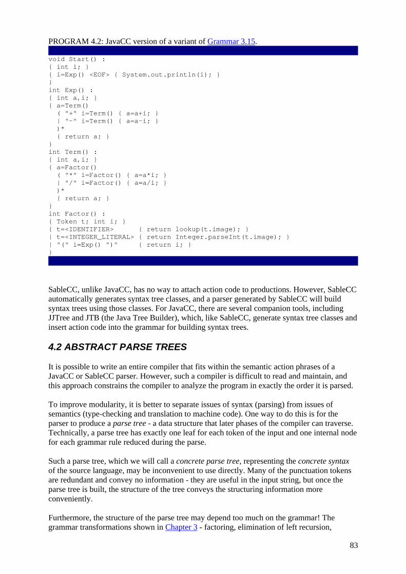
83

PROGRAM 4.2: JavaCC version of a variant of Grammar 3.15. void Start() : { int i; } { i=Exp() <EOF> { System.out.println(i); } } int Exp() : { int a,i; } { a=Term() ( "+" i=Term() { a=a+i; } | "-" i=Term() { a=a-i; } )* { return a; } } int Term() : { int a,i; } { a=Factor() ( "*" i=Factor() { a=a*i; } | "/" i=Factor() { a=a/i; } )* { return a; } } int Factor() : { Token t; int i; } { t=<IDENTIFIER> { return lookup(t.image); } | t=<INTEGER_LITERAL> { return Integer.parseInt(t.image); } | "(" i=Exp() ")" { return i; } }

SableCC, unlike JavaCC, has no way to attach action code to productions. However, SableCC automatically generates syntax tree classes, and a parser generated by SableCC will build syntax trees using those classes. For JavaCC, there are several companion tools, including JJTree and JTB (the Java Tree Builder), which, like SableCC, generate syntax tree classes and insert action code into the grammar for building syntax trees.

4.2 ABSTRACT PARSE TREES

It is possible to write an entire compiler that fits within the semantic action phrases of a JavaCC or SableCC parser. However, such a compiler is difficult to read and maintain, and this approach constrains the compiler to analyze the program in exactly the order it is parsed.

To improve modularity, it is better to separate issues of syntax (parsing) from issues of semantics (type-checking and translation to machine code). One way to do this is for the parser to produce a parse tree - a data structure that later phases of the compiler can traverse. Technically, a parse tree has exactly one leaf for each token of the input and one internal node for each grammar rule reduced during the parse.

Such a parse tree, which we will call a concrete parse tree, representing the concrete syntax of the source language, may be inconvenient to use directly. Many of the punctuation tokens are redundant and convey no information - they are useful in the input string, but once the parse tree is built, the structure of the tree conveys the structuring information more conveniently.

Furthermore, the structure of the parse tree may depend too much on the grammar! The grammar transformations shown in Chapter 3 - factoring, elimination of left recursion,

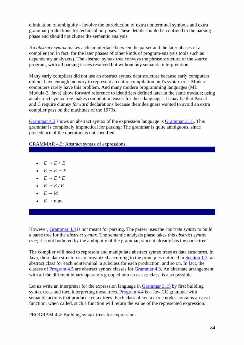
84

elimination of ambiguity - involve the introduction of extra nonterminal symbols and extra grammar productions for technical purposes. These details should be confined to the parsing phase and should not clutter the semantic analysis.

An abstract syntax makes a clean interface between the parser and the later phases of a compiler (or, in fact, for the later phases of other kinds of program-analysis tools such as dependency analyzers). The abstract syntax tree conveys the phrase structure of the source program, with all parsing issues resolved but without any semantic interpretation.

Many early compilers did not use an abstract syntax data structure because early computers did not have enough memory to represent an entire compilation unit's syntax tree. Modern computers rarely have this problem. And many modern programming languages (ML, Modula-3, Java) allow forward reference to identifiers defined later in the same module; using an abstract syntax tree makes compilation easier for these languages. It may be that Pascal and C require clumsy forward declarations because their designers wanted to avoid an extra compiler pass on the machines of the 1970s.

Grammar 4.3 shows an abstract syntax of the expression language is Grammar 3.15. This grammar is completely impractical for parsing: The grammar is quite ambiguous, since precedence of the operators is not specified.

GRAMMAR 4.3: Abstract syntax of expressions.

• E → E + E • E → E − E • E → E * E • E → E / E • E → id • E → num

However, Grammar 4.3 is not meant for parsing. The parser uses the concrete syntax to build a parse tree for the abstract syntax. The semantic analysis phase takes this abstract syntax tree; it is not bothered by the ambiguity of the grammar, since it already has the parse tree!

The compiler will need to represent and manipulate abstract syntax trees as data structures. In Java, these data structures are organized according to the principles outlined in Section 1.3: an abstract class for each nonterminal, a subclass for each production, and so on. In fact, the classes of Program 4.5 are abstract syntax classes for Grammar 4.3. An alternate arrangement, with all the different binary operators grouped into an OpExp class, is also possible.

Let us write an interpreter for the expression language in Grammar 3.15 by first building syntax trees and then interpreting those trees. Program 4.4 is a JavaCC grammar with semantic actions that produce syntax trees. Each class of syntax-tree nodes contains an eval function; when called, such a function will return the value of the represented expression.

PROGRAM 4.4: Building syntax trees for expressions.

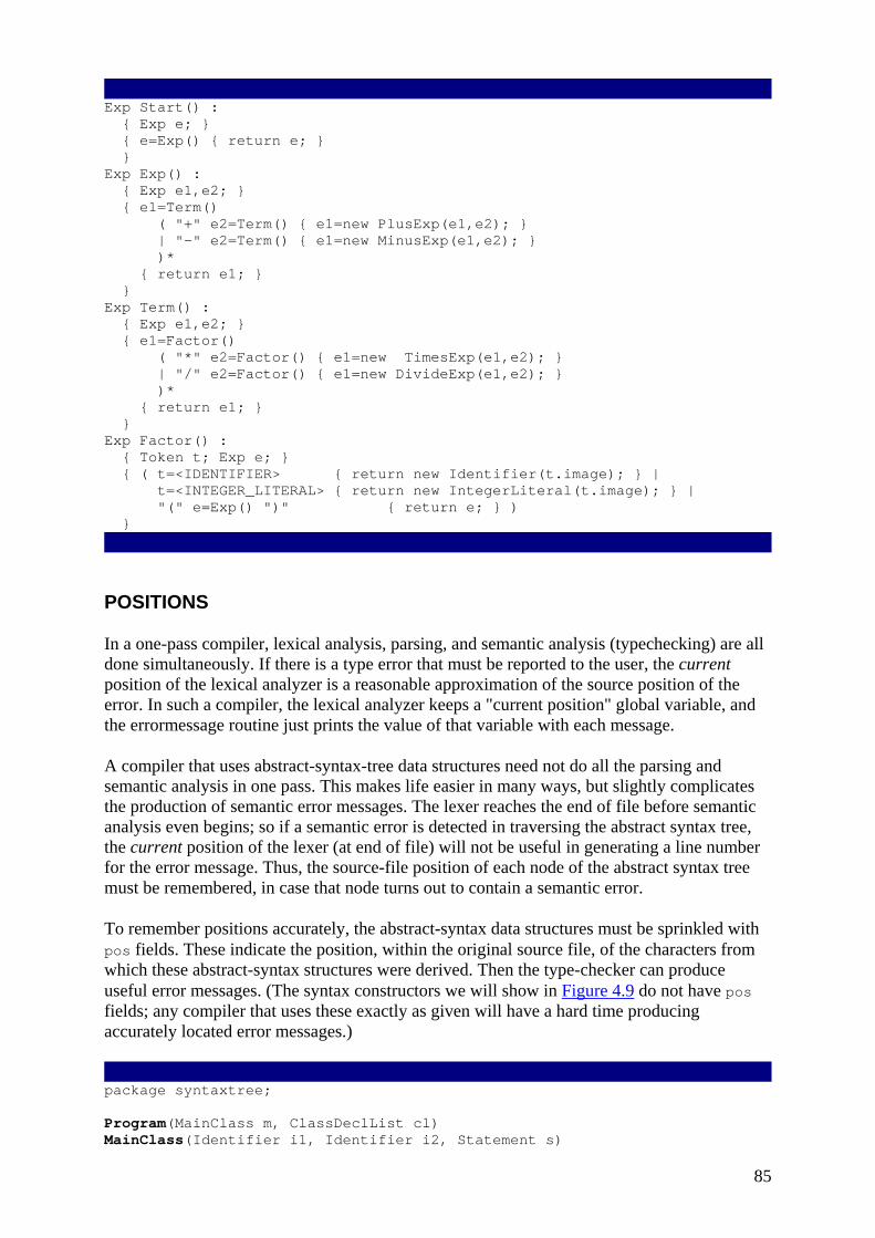
85

Exp Start() : { Exp e; } { e=Exp() { return e; } } Exp Exp() : { Exp e1,e2; } { e1=Term() ( "+" e2=Term() { e1=new PlusExp(e1,e2); } | "-" e2=Term() { e1=new MinusExp(e1,e2); } )* { return e1; } } Exp Term() : { Exp e1,e2; } { e1=Factor() ( "*" e2=Factor() { e1=new TimesExp(e1,e2); } | "/" e2=Factor() { e1=new DivideExp(e1,e2); } )* { return e1; } } Exp Factor() : { Token t; Exp e; } { ( t=<IDENTIFIER> { return new Identifier(t.image); } | t=<INTEGER_LITERAL> { return new IntegerLiteral(t.image); } | "(" e=Exp() ")" { return e; } ) }

POSITIONS

In a one-pass compiler, lexical analysis, parsing, and semantic analysis (typechecking) are all done simultaneously. If there is a type error that must be reported to the user, the current position of the lexical analyzer is a reasonable approximation of the source position of the error. In such a compiler, the lexical analyzer keeps a "current position" global variable, and the errormessage routine just prints the value of that variable with each message.

A compiler that uses abstract-syntax-tree data structures need not do all the parsing and semantic analysis in one pass. This makes life easier in many ways, but slightly complicates the production of semantic error messages. The lexer reaches the end of file before semantic analysis even begins; so if a semantic error is detected in traversing the abstract syntax tree, the current position of the lexer (at end of file) will not be useful in generating a line number for the error message. Thus, the source-file position of each node of the abstract syntax tree must be remembered, in case that node turns out to contain a semantic error.

To remember positions accurately, the abstract-syntax data structures must be sprinkled with pos fields. These indicate the position, within the original source file, of the characters from which these abstract-syntax structures were derived. Then the type-checker can produce useful error messages. (The syntax constructors we will show in Figure 4.9 do not have pos fields; any compiler that uses these exactly as given will have a hard time producing accurately located error messages.)

package syntaxtree; Program(MainClass m, ClassDeclList cl) MainClass(Identifier i1, Identifier i2, Statement s)

86

abstract class ClassDecl ClassDeclSimple(Identifier i, VarDeclList vl, MethodDeclList ml) ClassDeclExtends(Identifier i, Identifier j, VarDeclList vl, MethodDeclList ml) see Ch.14 VarDecl(Type t, Identifier i) MethodDecl(Type t, Identifier i, FormalList fl, VarDeclList vl, StatementList sl, Exp e) Formal(Type t, Identifier i) abstract class Type IntArrayType() BooleanType() IntegerType() IdentifierType(String s) abstract class Statement Block(StatementList sl) If(Exp e, Statement s1, Statement s2) While(Exp e, Statement s) Print(Exp e) Assign(Identifier i, Exp e) ArrayAssign(Identifier i, Exp e1, Exp e2) abstract class Exp And(Exp e1, Exp e2) LessThan(Exp e1, Exp e2) Plus(Exp e1, Exp e2) Minus(Exp e1, Exp e2) Times(Exp e1, Exp e2) ArrayLookup(Exp e1, Exp e2) ArrayLength(Exp e) Call(Exp e, Identifier i, ExpList el) IntegerLiteral(int i) True() False() IdentifierExp(String s) This() NewArray(Exp e) NewObject(Identifier i) Not(Exp e) Identifier(String s) list classes ClassDeclList() ExpList() FormalList() MethodDeclList() StatementList() VarDeclList()

Figure 4.9: Abstract syntax for the MiniJava language.

The lexer must pass the source-file positions of the beginning and end of each token to the parser. We can augment the types Exp, etc. with a position field; then each constructor must take a pos argument to initialize this field. The positions of leaf nodes of the syntax tree can be obtained from the tokens returned by the lexical analyzer; internal-node positions can be derived from the positions of their subtrees. This is tedious but straightforward.

4.3 VISITORS

Each abstract syntax class of Program 4.5 has a constructor for building syntax trees, and an eval method for returning the value of the represented expression. This is an object-oriented style of programming. Let us consider an alternative.

PROGRAM 4.5: Exp class for Program 4.4.

87

public abstract class Exp { public abstract int eval(); } public class PlusExp extends Exp { private Exp e1,e2; public PlusExp(Exp a1, Exp a2) { e1=a1; e2=a2; } public int eval() { return e1.eval()+e2.eval(); } } public class MinusExp extends Exp { private Exp e1,e2; public MinusExp(Exp a1, Exp a2) { e1=a1; e2=a2; } public int eval() { return e1.eval()-e2.eval(); } } public class TimesExp extends Exp { private Exp e1,e2; public TimesExp(Exp a1, Exp a2) { e1=a1; e2=a2; } public int eval() { return e1.eval()*e2.eval(); } } public class DivideExp extends Exp { private Exp e1,e2; public DivideExp(Exp a1, Exp a2) { e1=a1; e2=a2; } public int eval() { return e1.eval()/e2.eval(); } } public class Identifier extends Exp { private String f0; public Identifier(String n0) { f0 = n0; } public int eval() { return lookup(f0); } } public class IntegerLiteral extends Exp { private String f0; public IntegerLiteral(String n0) { f0 = n0; } public int eval() { return Integer.parseInt(f0); } }

Suppose the code for evaluating expressions is written separately from the abstract syntax classes. We might do that by examining the syntax-tree data structure by using instanceof and by fetching public class variables that represent subtrees. This is a syntax separate from interpretations style of programming.

The choice of style affects the modularity of the compiler. In a situation such as this, we have several kinds of objects: compound statements, assignment statements, print statements, and so on. And we also may have several different interpretations of these objects: type-check, translate to Pentium code, translate to Sparc code, optimize, interpret, and so on.

Each interpretation must be applied to each kind; if we add a new kind, we must implement each interpretation for it; and if we add a new interpretation, we must implement it for each kind. Figure 4.6 illustrates the orthogonality of kinds and interpretations - for compilers, and

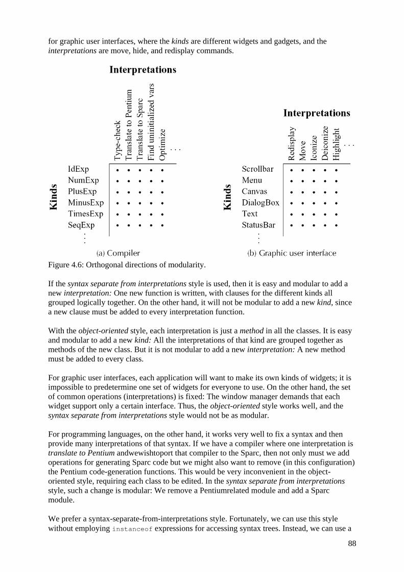
88

for graphic user interfaces, where the kinds are different widgets and gadgets, and the interpretations are move, hide, and redisplay commands.

Figure 4.6: Orthogonal directions of modularity.

If the syntax separate from interpretations style is used, then it is easy and modular to add a new interpretation: One new function is written, with clauses for the different kinds all grouped logically together. On the other hand, it will not be modular to add a new kind, since a new clause must be added to every interpretation function.

With the object-oriented style, each interpretation is just a method in all the classes. It is easy and modular to add a new kind: All the interpretations of that kind are grouped together as methods of the new class. But it is not modular to add a new interpretation: A new method must be added to every class.

For graphic user interfaces, each application will want to make its own kinds of widgets; it is impossible to predetermine one set of widgets for everyone to use. On the other hand, the set of common operations (interpretations) is fixed: The window manager demands that each widget support only a certain interface. Thus, the object-oriented style works well, and the syntax separate from interpretations style would not be as modular.

For programming languages, on the other hand, it works very well to fix a syntax and then provide many interpretations of that syntax. If we have a compiler where one interpretation is translate to Pentium andwewishtoport that compiler to the Sparc, then not only must we add operations for generating Sparc code but we might also want to remove (in this configuration) the Pentium code-generation functions. This would be very inconvenient in the object-oriented style, requiring each class to be edited. In the syntax separate from interpretations style, such a change is modular: We remove a Pentiumrelated module and add a Sparc module.

We prefer a syntax-separate-from-interpretations style. Fortunately, we can use this style without employing instanceof expressions for accessing syntax trees. Instead, we can use a

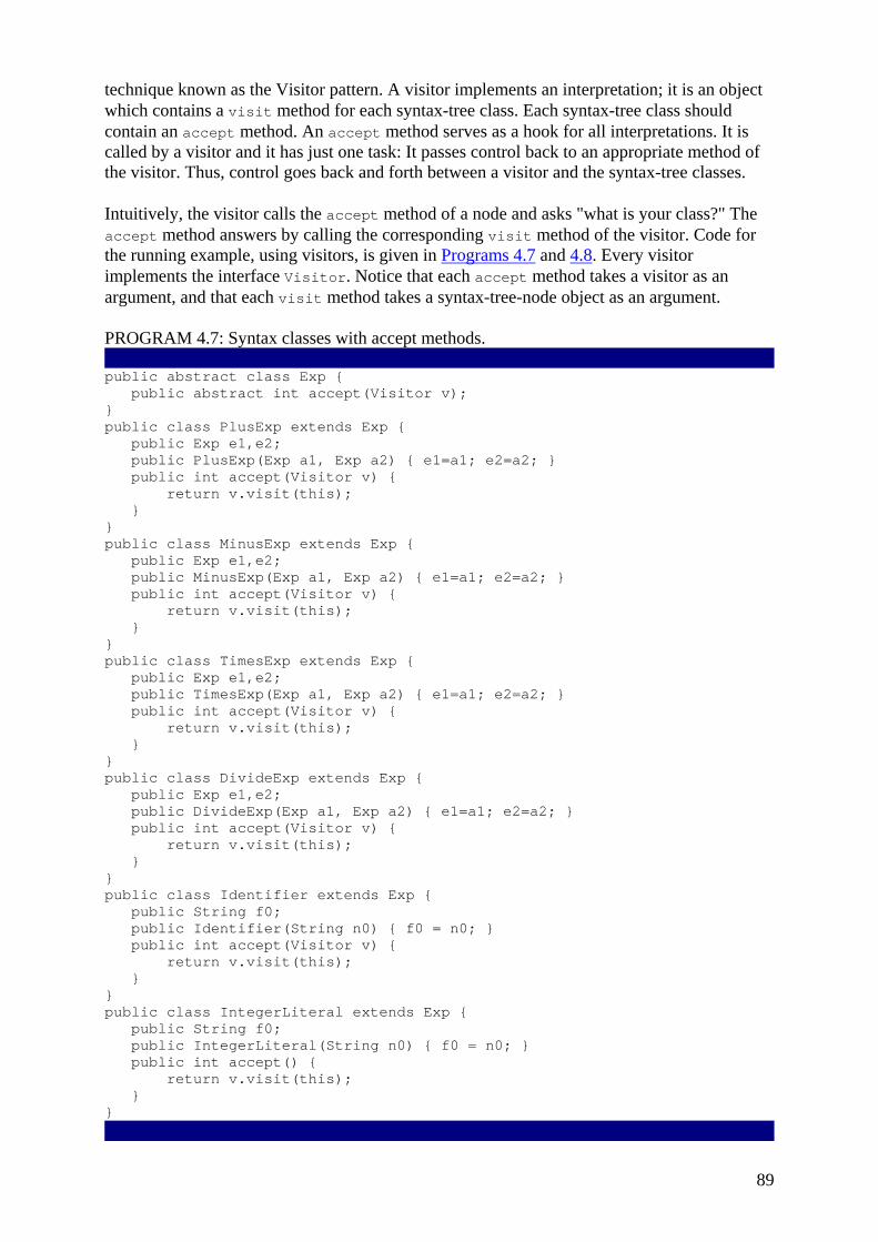
89

technique known as the Visitor pattern. A visitor implements an interpretation; it is an object which contains a visit method for each syntax-tree class. Each syntax-tree class should contain an accept method. An accept method serves as a hook for all interpretations. It is called by a visitor and it has just one task: It passes control back to an appropriate method of the visitor. Thus, control goes back and forth between a visitor and the syntax-tree classes.

Intuitively, the visitor calls the accept method of a node and asks "what is your class?" The accept method answers by calling the corresponding visit method of the visitor. Code for the running example, using visitors, is given in Programs 4.7 and 4.8. Every visitor implements the interface Visitor. Notice that each accept method takes a visitor as an argument, and that each visit method takes a syntax-tree-node object as an argument.

PROGRAM 4.7: Syntax classes with accept methods. public abstract class Exp { public abstract int accept(Visitor v); } public class PlusExp extends Exp { public Exp e1,e2; public PlusExp(Exp a1, Exp a2) { e1=a1; e2=a2; } public int accept(Visitor v) { return v.visit(this); } } public class MinusExp extends Exp { public Exp e1,e2; public MinusExp(Exp a1, Exp a2) { e1=a1; e2=a2; } public int accept(Visitor v) { return v.visit(this); } } public class TimesExp extends Exp { public Exp e1,e2; public TimesExp(Exp a1, Exp a2) { e1=a1; e2=a2; } public int accept(Visitor v) { return v.visit(this); } } public class DivideExp extends Exp { public Exp e1,e2; public DivideExp(Exp a1, Exp a2) { e1=a1; e2=a2; } public int accept(Visitor v) { return v.visit(this); } } public class Identifier extends Exp { public String f0; public Identifier(String n0) { f0 = n0; } public int accept(Visitor v) { return v.visit(this); } } public class IntegerLiteral extends Exp { public String f0; public IntegerLiteral(String n0) { f0 = n0; } public int accept() { return v.visit(this); } }

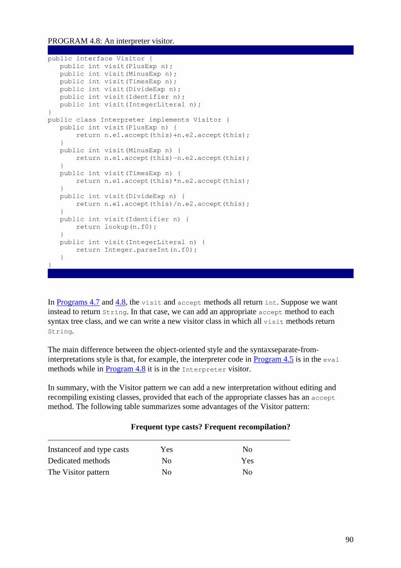
90

PROGRAM 4.8: An interpreter visitor. public interface Visitor { public int visit(PlusExp n); public int visit(MinusExp n); public int visit(TimesExp n); public int visit(DivideExp n); public int visit(Identifier n); public int visit(IntegerLiteral n); } public class Interpreter implements Visitor { public int visit(PlusExp n) { return n.e1.accept(this)+n.e2.accept(this); } public int visit(MinusExp n) { return n.e1.accept(this)-n.e2.accept(this); } public int visit(TimesExp n) { return n.e1.accept(this)*n.e2.accept(this); } public int visit(DivideExp n) { return n.e1.accept(this)/n.e2.accept(this); } public int visit(Identifier n) { return lookup(n.f0); } public int visit(IntegerLiteral n) { return Integer.parseInt(n.f0); } }

In Programs 4.7 and 4.8, the visit and accept methods all return int. Suppose we want instead to return String. In that case, we can add an appropriate accept method to each syntax tree class, and we can write a new visitor class in which all visit methods return String.

The main difference between the object-oriented style and the syntaxseparate-from-interpretations style is that, for example, the interpreter code in Program 4.5 is in the eval methods while in Program 4.8 it is in the Interpreter visitor.

In summary, with the Visitor pattern we can add a new interpretation without editing and recompiling existing classes, provided that each of the appropriate classes has an accept method. The following table summarizes some advantages of the Visitor pattern:

Frequent type casts? Frequent recompilation?

Instanceof and type casts Yes No Dedicated methods No Yes The Visitor pattern No No

91

ABSTRACT SYNTAX FOR MiniJava

Figure 4.9 shows classes for the abstract syntax of MiniJava. The meaning of each constructor in the abstract syntax should be clear after a careful study of Appendix A, but there are a few points that merit explanation.

Only the constructors are shown in Figure 4.9; the object field variables correspond exactly to the names of the constructor arguments. Each of the six list classes is implemented in the same way, for example:

public class ExpList { private Vector list; public ExpList() { list = new Vector(); } public void addElement(Exp n) { list.addElement(n); } public Exp elementAt(int i) { return (Exp)list.elementAt(i); } public int size() { return list.size(); } }

Each of the nonlist classes has an accept method for use with the visitor pattern. The interface Visitor is shown in Program 4.10.

PROGRAM 4.10: MiniJava visitor public interface Visitor { public void visit(Program n); public void visit(MainClass n); public void visit(ClassDeclSimple n); public void visit(ClassDeclExtends n); public void visit(VarDecl n); public void visit(MethodDecl n); public void visit(Formal n); public void visit(IntArrayType n); public void visit(BooleanType n); public void visit(IntegerType n); public void visit(IdentifierType n); public void visit(Block n); public void visit(If n); public void visit(While n); public void visit(Print n); public void visit(Assign n); public void visit(ArrayAssign n); public void visit(And n); public void visit(LessThan n); public void visit(Plus n); public void visit(Minus n); public void visit(Times n); public void visit(ArrayLookup n); public void visit(ArrayLength n); public void visit(Call n); public void visit(IntegerLiteral n); public void visit(True n); public void visit(False n); public void visit(IdentifierExp n);

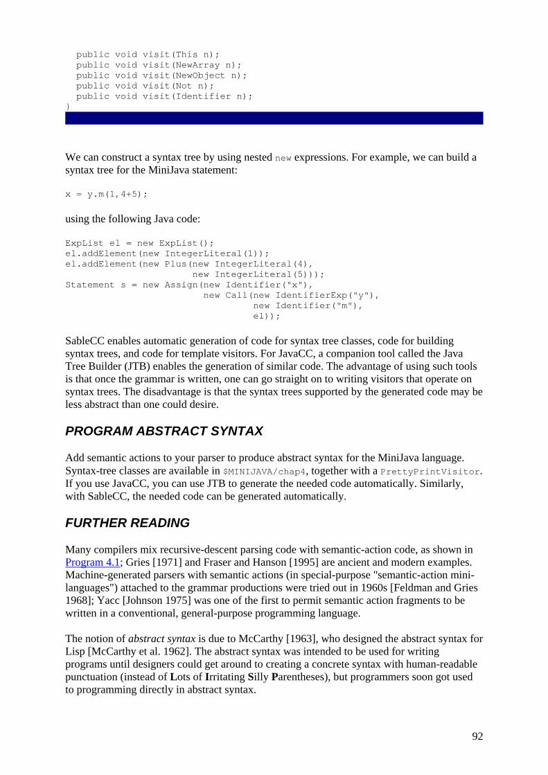
92

public void visit(This n); public void visit(NewArray n); public void visit(NewObject n); public void visit(Not n); public void visit(Identifier n); }

We can construct a syntax tree by using nested new expressions. For example, we can build a syntax tree for the MiniJava statement:

x = y.m(1,4+5);

using the following Java code:

ExpList el = new ExpList(); el.addElement(new IntegerLiteral(1)); el.addElement(new Plus(new IntegerLiteral(4), new IntegerLiteral(5))); Statement s = new Assign(new Identifier("x"), new Call(new IdentifierExp("y"), new Identifier("m"), el));

SableCC enables automatic generation of code for syntax tree classes, code for building syntax trees, and code for template visitors. For JavaCC, a companion tool called the Java Tree Builder (JTB) enables the generation of similar code. The advantage of using such tools is that once the grammar is written, one can go straight on to writing visitors that operate on syntax trees. The disadvantage is that the syntax trees supported by the generated code may be less abstract than one could desire.

PROGRAM ABSTRACT SYNTAX

Add semantic actions to your parser to produce abstract syntax for the MiniJava language. Syntax-tree classes are available in $MINIJAVA/chap4, together with a PrettyPrintVisitor. If you use JavaCC, you can use JTB to generate the needed code automatically. Similarly, with SableCC, the needed code can be generated automatically.

FURTHER READING

Many compilers mix recursive-descent parsing code with semantic-action code, as shown in Program 4.1; Gries [1971] and Fraser and Hanson [1995] are ancient and modern examples. Machine-generated parsers with semantic actions (in special-purpose "semantic-action mini-languages") attached to the grammar productions were tried out in 1960s [Feldman and Gries 1968]; Yacc [Johnson 1975] was one of the first to permit semantic action fragments to be written in a conventional, general-purpose programming language.

The notion of abstract syntax is due to McCarthy [1963], who designed the abstract syntax for Lisp [McCarthy et al. 1962]. The abstract syntax was intended to be used for writing programs until designers could get around to creating a concrete syntax with human-readable punctuation (instead of Lots of Irritating Silly Parentheses), but programmers soon got used to programming directly in abstract syntax.

93

The search for a theory of programming-language semantics, and a notation for expressing semantics in a compiler-compiler, led to ideas such as denotational semantics [Stoy 1977]. The semantic interpreter shown in Programs 4.4 and 4.5 is inspired by ideas from denotational semantics, as is the idea of separating concrete syntax from semantics using the abstract syntax as a clean interface.

EXERCISES 4.1 Write a package of Java classes to express the abstract syntax of regular expressions. 4.2 Extend Grammar 3.15 such that a program is a sequence of either assignment statements

or print statements. Each assignment statement assigns an expression to an implicitly-declared variable; each print statement prints the value of an expression. Extend the interpreter in Program 4.1 to handle the new language.

4.3 Write a JavaCC version of the grammar from Exercise 4.2. Insert Java code for

interpreting programs, in the style of Program 4.2. 4.4 Modify the JavaCC grammar from Exercise 4.3 to contain Java code for building syntax

trees, in the style of Program 4.4. Write two interpreters for the language: one in object-oriented style and one that uses visitors.

4.5 In $MINIJAVA/chap4/handcrafted/visitor, there is a file with a visitor

PrettyPrintVisitor.java for pretty printing syntax trees. Improve the pretty printing of nested if and while statements.

4.6 The visitor pattern in Program 4.7 has accept methods that return int. Ifone wanted to

write some visitors that return integers, others that return class A, and yet others that return class B, one could modify all the classes in Program 4.7 to add two more accept methods, but this would not be very modular. Another way is to make the visitor return Object and cast each result, but this loses the benefit of compile-time type-checking. But there is a third way.

Modify Program 4.7 so that all the accept methods return void, and write two extensions of the Visitor class: one that computes an int for each Exp, and the other that computes a float for each Exp. Since the accept method will return void, the visitor object must have an instance variable into which each accept method can place its result. Explain why, if one then wanted to write a visitor that computed an object of class C for each Exp, no more modification of the Exp subclasses would be necessary.

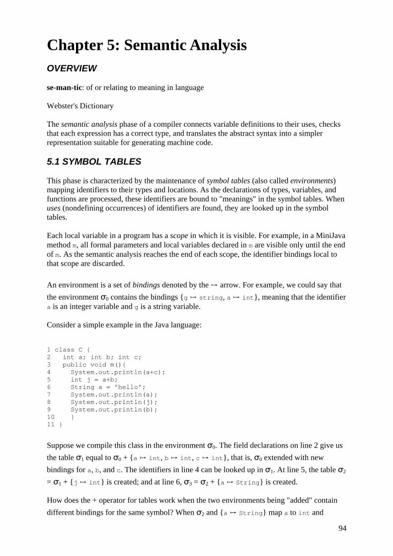
94

Chapter 5: Semantic Analysis OVERVIEW

se-man-tic: of or relating to meaning in language


The semantic analysis phase of a compiler connects variable definitions to their uses, checks that each expression has a correct type, and translates the abstract syntax into a simpler representation suitable for generating machine code.

5.1 SYMBOL TABLES

This phase is characterized by the maintenance of symbol tables (also called environments) mapping identifiers to their types and locations. As the declarations of types, variables, and functions are processed, these identifiers are bound to "meanings" in the symbol tables. When uses (nondefining occurrences) of identifiers are found, they are looked up in the symbol tables.

Each local variable in a program has a scope in which it is visible. For example, in a MiniJava method m, all formal parameters and local variables declared in m are visible only until the end of m. As the semantic analysis reaches the end of each scope, the identifier bindings local to that scope are discarded.

An environment is a set of bindings denoted by the ↦ arrow. For example, we could say that the environment σ0 contains the bindings {g ↦ string, a ↦ int}, meaning that the identifier a is an integer variable and g is a string variable.

Consider a simple example in the Java language:

1 class C { 2 int a; int b; int c; 3 public void m(){ 4 System.out.println(a+c); 5 int j = a+b; 6 String a = "hello"; 7 System.out.println(a); 8 System.out.println(j); 9 System.out.println(b); 10 } 11 }

Suppose we compile this class in the environment σ0. The field declarations on line 2 give us the table σ1 equal to σ0 + {a ↦ int, b ↦ int, c ↦ int}, that is, σ0 extended with new bindings for a, b, and c. The identifiers in line 4 can be looked up in σ1. At line 5, the table σ2 = σ1 + {j ↦ int} is created; and at line 6, σ3 = σ2 + {a ↦ String} is created.

How does the + operator for tables work when the two environments being "added" contain different bindings for the same symbol? When σ2 and {a ↦ String} map a to int and

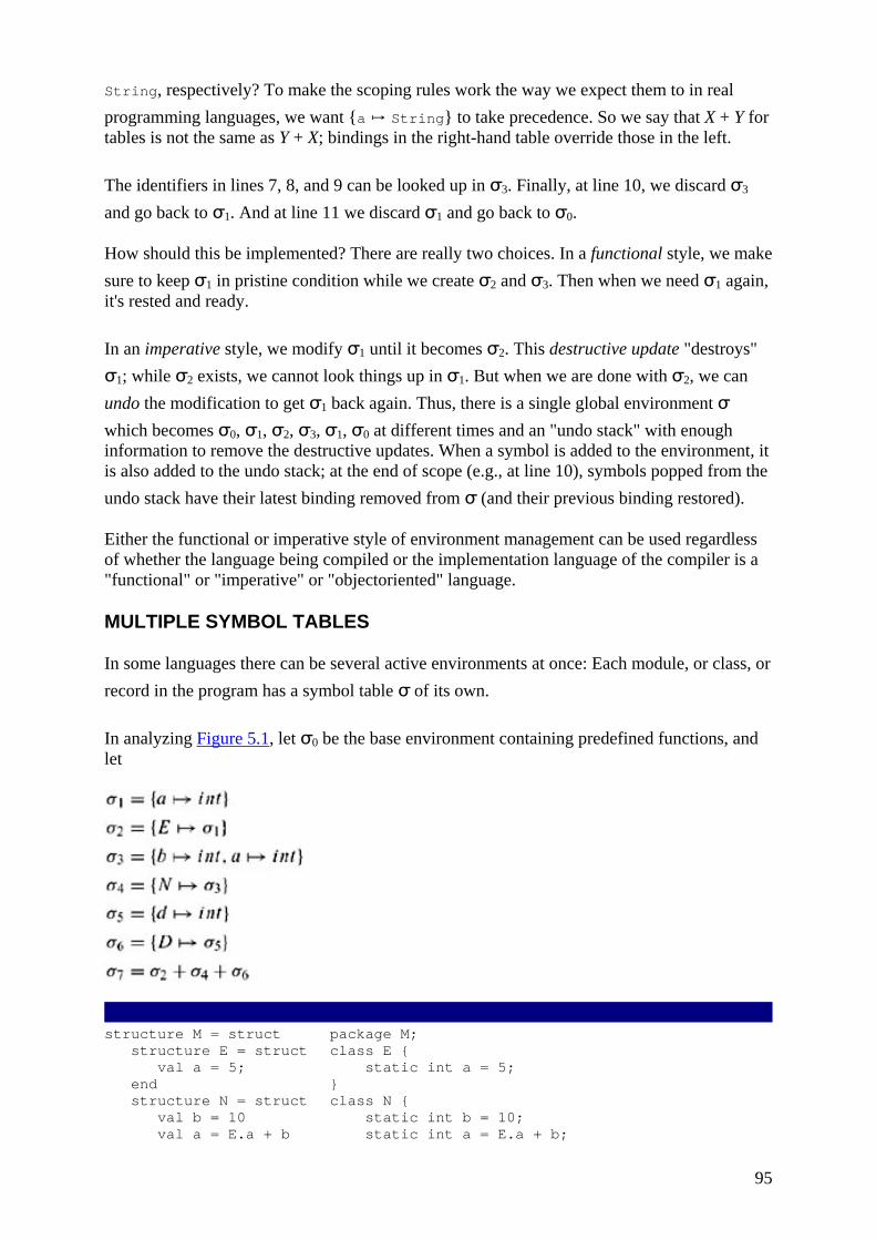
95

String, respectively? To make the scoping rules work the way we expect them to in real programming languages, we want {a ↦ String} to take precedence. So we say that X + Y for tables is not the same as Y + X; bindings in the right-hand table override those in the left.

The identifiers in lines 7, 8, and 9 can be looked up in σ3. Finally, at line 10, we discard σ3 and go back to σ1. And at line 11 we discard σ1 and go back to σ0.

How should this be implemented? There are really two choices. In a functional style, we make sure to keep σ1 in pristine condition while we create σ2 and σ3. Then when we need σ1 again, it's rested and ready.

In an imperative style, we modify σ1 until it becomes σ2. This destructive update "destroys" σ1; while σ2 exists, we cannot look things up in σ1. But when we are done with σ2, we can undo the modification to get σ1 back again. Thus, there is a single global environment σ which becomes σ0, σ1, σ2, σ3, σ1, σ0 at different times and an "undo stack" with enough information to remove the destructive updates. When a symbol is added to the environment, it is also added to the undo stack; at the end of scope (e.g., at line 10), symbols popped from the undo stack have their latest binding removed from σ (and their previous binding restored).

Either the functional or imperative style of environment management can be used regardless of whether the language being compiled or the implementation language of the compiler is a "functional" or "imperative" or "objectoriented" language.

MULTIPLE SYMBOL TABLES

In some languages there can be several active environments at once: Each module, or class, or record in the program has a symbol table σ of its own.

In analyzing Figure 5.1, let σ0 be the base environment containing predefined functions, and let

structure M = struct structure E = struct val a = 5; end structure N = struct val b = 10 val a = E.a + b

package M; class E { static int a = 5; } class N { static int b = 10; static int a = E.a + b;

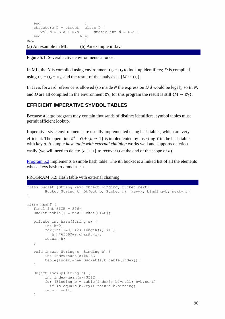
96

end structure D = struct val d = E.a + N.a end end

} class D { static int d = E.a + N.a; }

(a) An example in ML (b) An example in Java Figure 5.1: Several active environments at once.

In ML, the N is compiled using environment σ0 + σ2 to look up identifiers; D is compiled using σ0 + σ2 + σ4, and the result of the analysis is {M ↦ σ7}.

In Java, forward reference is allowed (so inside N the expression D.d would be legal), so E, N, and D are all compiled in the environment σ7; for this program the result is still {M ↦ σ7}.

EFFICIENT IMPERATIVE SYMBOL TABLES

Because a large program may contain thousands of distinct identifiers, symbol tables must permit efficient lookup.

Imperative-style environments are usually implemented using hash tables, which are very efficient. The operation σ′ = σ + {a ↦ τ} is implemented by inserting τ in the hash table with key a. A simple hash table with external chaining works well and supports deletion easily (we will need to delete {a ↦ τ} to recover σ at the end of the scope of a).

Program 5.2 implements a simple hash table. The ith bucket is a linked list of all the elements whose keys hash to i mod SIZE.

PROGRAM 5.2: Hash table with external chaining. class Bucket {String key; Object binding; Bucket next; Bucket(String k, Object b, Bucket n) {key=k; binding=b; next=n;} } class HashT { final int SIZE = 256; Bucket table[] = new Bucket[SIZE]; private int hash(String s) { int h=0; for(int i=0; i<s.length(); i++) h=h*65599+s.charAt(i); return h; } void insert(String s, Binding b) { int index=hash(s)%SIZE table[index]=new Bucket(s,b,table[index]); } Object lookup(String s) { int index=hash(s)%SIZE for (Binding b = table[index]; b!=null; b=b.next) if (s.equals(b.key)) return b.binding; return null; }

97

void pop(String s) { int index=hash(s)%SIZE table[index]=table[index].next; } }

Consider σ + {a ↦ τ2} when σ contains a ↦ τ1 already. The insert function leaves a ↦ τ1 in the bucket and puts a ↦ τ2 earlier in the list. Then, when pop(a) is done at the end of a's scope, σ is restored. Of course, pop works only if bindings are inserted and popped in a stacklike fashion.

An industrial-strength implementation would improve on this in several ways; see Exercise 5.1.

EFFICIENT FUNCTIONAL SYMBOL TABLES

In the functional style, we wish to compute σ′ = σ + {a ↦ τ} in such a way that we still have σ available to look up identifiers. Thus, instead of "altering" a table by adding a binding to it we create a new table by computing the "sum" of an existing table and a new binding. Similarly, when we add 7 + 8 we don't alter the 7 by adding 8 to it; we create a new value, 15 − and the 7 is still available for other computations.

However, nondestructive update is not efficient for hash tables. Figure 5.3a shows a hash table implementing mapping m1. It is fast and efficient to add mouse to the fifth slot; just make the mouse record point at the (old) head of the fifth linked list, and make the fifth slot point to the mouse record. But then we no longer have the mapping m1:Wehavedestroyedittomake m2. The other alternative is to copy the array, but still share all the old buckets, as shown in Figure 5.3b. But this is not efficient: The array in a hash table should be quite large, proportional in size to the number of elements, and we cannot afford to copy it for each new entry in the table.

Figure 5.3: Hash tables.

98

By using binary search trees we can perform such "functional" additions to search trees efficiently. Consider, for example, the search tree in Figure 5.4, which represents the mapping

Figure 5.4: Binary search trees.

We can add the binding mouse ↦ 4, creating the mapping m2 without destroying the mapping m1, as shown in Figure 5.4b. If we add a new node at depth d of the tree, we must create d new nodes - but we don't need to copy the whole tree. So creating a new tree (that shares some structure with the old one) can be done as efficiently as looking up an element: in log(n) time for a balanced tree of n nodes. This is an example of a persistent data structure; a persistent red-black tree can be kept balanced to guarantee log(n) access time (see Exercise 1.1c, and also page 276).

SYMBOLS

The hash table of Program 5.2 must examine every character of the string s for the hash operation, and then again each time it compares s against a string in the ith bucket. To avoid unnecessary string comparisons, we can convert each string to a symbol, so that all the different occurrences of any given string convert to the same symbol object.

The Symbol module implements symbols and has these important properties:

• Comparing symbols for equality is fast (just pointer or integer comparison). • Extracting an integer hash key is fast (in case we want to make a hash table mapping

symbols to something else). • Comparing two symbols for "greater-than" (in some arbitrary ordering) is fast (in case

we want to make binary search trees).

Even if we intend to make functional-style environments mapping symbols to bindings, we can use a destructive-update hash table to map strings to symbols: We need this to make sure

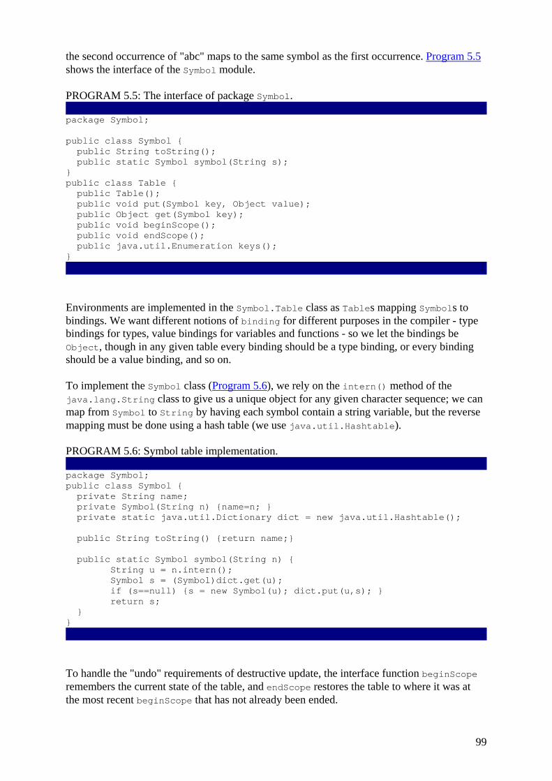
99

the second occurrence of "abc" maps to the same symbol as the first occurrence. Program 5.5 shows the interface of the Symbol module.

PROGRAM 5.5: The interface of package Symbol. package Symbol; public class Symbol { public String toString(); public static Symbol symbol(String s); } public class Table { public Table(); public void put(Symbol key, Object value); public Object get(Symbol key); public void beginScope(); public void endScope(); public java.util.Enumeration keys(); }

Environments are implemented in the Symbol.Table class as Tables mapping Symbols to bindings. We want different notions of binding for different purposes in the compiler - type bindings for types, value bindings for variables and functions - so we let the bindings be Object, though in any given table every binding should be a type binding, or every binding should be a value binding, and so on.

To implement the Symbol class (Program 5.6), we rely on the intern() method of the java.lang.String class to give us a unique object for any given character sequence; we can map from Symbol to String by having each symbol contain a string variable, but the reverse mapping must be done using a hash table (we use java.util.Hashtable).

PROGRAM 5.6: Symbol table implementation. package Symbol; public class Symbol { private String name; private Symbol(String n) {name=n; } private static java.util.Dictionary dict = new java.util.Hashtable(); public String toString() {return name;} public static Symbol symbol(String n) { String u = n.intern(); Symbol s = (Symbol)dict.get(u); if (s==null) {s = new Symbol(u); dict.put(u,s); } return s; } }

To handle the "undo" requirements of destructive update, the interface function beginScope remembers the current state of the table, and endScope restores the table to where it was at the most recent beginScope that has not already been ended.

100

An imperative table is implemented using a hash table. When the binding x ↦ b is entered (table.put(x,b)), x is hashed into an index i, and a Binder object x ↦ b is placed at the head of the linked list for the ith bucket. If the table had already contained a binding x ↦ b′, that would still be in the bucket, hidden by x ↦ b. This is important because it will support the implementation of undo (beginScope and endScope).

The key x is not a character string, but is the Symbol object itself.

There must also be an auxiliary stack, showing in what order the symbols were "pushed" into the symbol table. When x ↦ b is entered, then x is pushed onto this stack. A beginScope operation pushes a special marker onto the stack. Then, to implement endScope, symbols are popped off the stack down to and including the topmost marker. As each symbol is popped, the head binding in its bucket is removed.

The auxiliary stack can be integrated into the Binder by having a global variable top showing the most recent Symbol bound in the table. Then "pushing" is accomplished by copying top into the prevtop field of the Binder. Thus, the "stack" is threaded through the binders.

If we wanted to use functional-style symbol tables, the Table interface might look like this:

public class Table { public Table(); public Table put(Symbol key, Object value); public Object get(Symbol key); public java.util.Enumeration keys(); }

The put function would return a new table without modifying the old one. We wouldn't need beginScope and endScope, because we could keep an old version of the table even as we use the new version.

5.2 TYPE-CHECKING MiniJava

With what should a symbol table be filled - that is, what is a binding? To enable type-checking of MiniJava programs, the symbol table should contain all declared type information:

• each variable name and formal-parameter name should be bound to its type; • each method name should be bound to its parameters, result type, and local variables;

and • each class name should be bound to its variable and method declarations.

For example, consider Figure 5.7, which shows a program and its symbol table. The two class names B and C are each mapped to two tables for fields and methods. In turn, each method is mapped to both its result type and tables with its formal parameters and local variables.

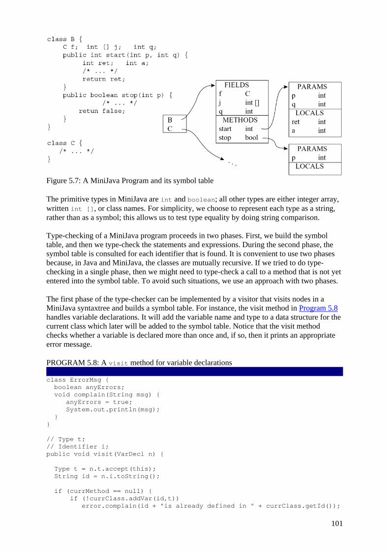
101

Figure 5.7: A MiniJava Program and its symbol table

The primitive types in MiniJava are int and boolean; all other types are either integer array, written int [], or class names. For simplicity, we choose to represent each type as a string, rather than as a symbol; this allows us to test type equality by doing string comparison.

Type-checking of a MiniJava program proceeds in two phases. First, we build the symbol table, and then we type-check the statements and expressions. During the second phase, the symbol table is consulted for each identifier that is found. It is convenient to use two phases because, in Java and MiniJava, the classes are mutually recursive. If we tried to do type-checking in a single phase, then we might need to type-check a call to a method that is not yet entered into the symbol table. To avoid such situations, we use an approach with two phases.

The first phase of the type-checker can be implemented by a visitor that visits nodes in a MiniJava syntaxtree and builds a symbol table. For instance, the visit method in Program 5.8 handles variable declarations. It will add the variable name and type to a data structure for the current class which later will be added to the symbol table. Notice that the visit method checks whether a variable is declared more than once and, if so, then it prints an appropriate error message.

PROGRAM 5.8: A visit method for variable declarations class ErrorMsg { boolean anyErrors; void complain(String msg) { anyErrors = true; System.out.println(msg); } } // Type t; // Identifier i; public void visit(VarDecl n) { Type t = n.t.accept(this); String id = n.i.toString(); if (currMethod == null) { if (!currClass.addVar(id,t)) error.complain(id + "is already defined in " + currClass.getId());

102

} else if (!currMethod.addVar(id,t)) error.complain(id + "is already defined in " + currClass.getId() + "." + currMethod.getId()); }

The second phase of the type-checker can be implemented by a visitor that type-checks all statements and expressions. The result type of each visit method is String, for representing MiniJava types. The idea is that when the visitor visits an expression, then it returns the type of that expression. If the expression does not type-check, then the type-check is terminated with an error message.

Let's take a simple case: an addition expression e1 + e2. In MiniJava, both operands must be integers (the type-checker must check this) and the result will be an integer (the type-checker will return this type). The visit method for addition is easy to implement; see Program 5.9.

PROGRAM 5.9: A visit method for plus expressions // Exp e1,e2; public Type visit(Plus n) { if (! (n.e1.accept(this) instanceof IntegerType) ) error.complain("Left side of LessThan must be of type integer"); if (! (n.e2.accept(this) instanceof IntegerType) ) error.complain("Right side of LessThan must be of type integer"); return new IntegerType(); }

In most languages, addition is overloaded: The + operator stands for either integer addition or real addition. If the operands are both integers, the result is integer; if the operands are both real, the result is real. And in many languages if one operand is an integer and the other is real, the integer is implicitly converted into a real, and the result is real. Of course, the compiler will have to make this conversion explicit in the machine code it generates.

For an assignment statement, it must be checked that the left-hand side and the right-hand side have the same type. When we allow extension of classes, the requirement is less strict: It is sufficient to check that the right-hand side is a subtype of the left-hand side.

For method calls, it is necessary to look up the method identifier in the symbol table to get the parameter list and the result type. For a call e.m(…), where e has type C, we look up the definition of m in class C. The parameter types must then be matched against the arguments in the function-call expression. The result type of the method becomes the type of the method call as a whole.

Every kind of statement and expression has its own type-checking rules, but in all the cases we have not already described, the rules can be derived by reference to the Java Language Specification.

ERROR HANDLING

When the type-checker detects a type error or an undeclared identifier, it should print an error message and continue - because the programmer would like to be told of all the errors in the

103

program. To recover after an error, it's often necessary to build data structures as if a valid expression had been encountered. For example, type-checking

{int i = new C(); int j = i + i; ... }

even though the expression new C() doesn't match the type required to initialize an integer, it is still useful to enter i in the symbol table as an integer so that the rest of the program can be type-checked.

If the type-checking phase detects errors, then the compiler should not produce a compiled program as output. This means that the later phases of the compiler - translation, register allocation, etc. - will not be executed. It will be easier to implement the later phases of the compiler if they are not required to handle invalid inputs. Thus, if at all possible, all errors in the input program should be detected in the front end of the compiler (parsing and type-checking).

PROGRAM TYPE-CHECKING

Design a set of visitors which type-checks a MiniJava program and produces any appropriate error messages about mismatching types or undeclared identifiers.

EXERCISES

• 5.1 Improve the hash table implementation of Program 5.2: Double the size of the array when the average bucket length grows larger than 2 (so table is now a pointer to a dynamically allocated array). To double an array, allocate a bigger one and rehash the contents of the old array; then discard the old array.

• ***5.2 In many applications, we want a + operator for environments that does more than add one new binding; instead of σ′ = σ + {a ↦ τ}, we want σ′ = σ1 + σ2, where σ1 and σ2 are arbitrary environments (perhaps overlapping, in which case bindings in σ2 take precedence).

We want an efficient algorithm and data structure for environment "adding." Balanced trees can implement σ + {a ↦ τ} efficiently (in log(N) time, where N is the size of σ), but take O(N) to compute σ1 + σ2 if σ1 and σ2 are both about size N.

To abstract the problem, solve the general nondisjoint integer-set union problem. The input is a set of commands of the form,

104

An efficient algorithm is one that can process an input of N commands, answering all membership queries, in less than o(N2) time.

• *a. Implement an algorithm that is efficient when a typical set union a ← b∪ c has b much smaller than c [Brown and Tarjan 1979].

• ***b. Design an algorithm that is efficient even in the worst case, or prove that this can't be done (see Lipton et al. [1997] for a lower bound in a restricted model).

105

Chapter 6: Activation Records stack: an orderly pile or heap


OVERVIEW

In almost any modern programming language, a function may have local variables that are created upon entry to the function. Several invocations of the function may exist at the same time, and each invocation has its own instantiations of local variables.

In the Java method

int f(int x) { int y = x+x; if (y<10) return f(y); else return y-1; }

a new instantiation of x is created (and initialized by f's caller) each time that f is called. Because there are recursive calls, many of these x's exist simultaneously. Similarly, a new instantiation of y is created each time the body of f is entered.

In many languages (including C, Pascal, and Java), local variables are destroyed when a function returns. Since a function returns only after all the functions it has called have returned, we say that function calls behave in last-in-first-out (LIFO) fashion. If local variables are created on function entry and destroyed on function exit, then we can use a LIFO data structure - a stack - to hold them.

HIGHER-ORDER FUNCTIONS

But in languages supporting both nested functions and function-valued variables, it may be necessary to keep local variables after a function has returned! Consider Program 6.1: This is legal in ML, but of course in C one cannot really nest the function g inside the function f.

PROGRAM 6.1: An example of higher-order functions. fun f(x) = let fun g(y) = x+y in g end val h = f(3) val j = f(4) val z = h(5) val w = j(7)

int (*)() f(int x) { int g(int y) {return x+y;} return g; } int (*h)() = f(3); int (*j)() = f(4); int z = h(5); int w = j(7);

(a) Written in ML (b) Written in pseudo-C

106

When f(3) is executed, a new local variable x is created for the activation of function f. Then g is returned as the result of f(x); but g has not yet been called, so y is not yet created.

At this point f has returned, but it is too early to destroy x, because when h(5) is eventually executed it will need the value x = 3. Meanwhile, f(4) is entered, creating a different instance of x, and it returns a different instance of g in which x = 4.

It is the combination of nested functions (where inner functions may use variables defined in the outer functions) and functions returned as results (or stored into variables) that causes local variables to need lifetimes longer than their enclosing function invocations.

Pascal has nested functions, but it does not have functions as returnable values. C has functions as returnable values, but not nested functions. So these languages can use stacks to hold local variables.

ML, Scheme, and several other languages have both nested functions and functions as returnable values (this combination is called higher-order functions). So they cannot use stacks to hold all local variables. This complicates the implementation of ML and Scheme - but the added expressive power of higher-order functions justifies the extra implementation effort.

For the remainder of this chapter we will consider languages with stackable local variables and postpone discussion of higher-order functions to Chapter 15. Notice that while Java allows nesting of functions (via inner classes), MiniJava does not.

6.1 STACK FRAMES

The simplest notion of a stack is a data structure that supports two operations, push and pop. However, it turns out that local variables are pushed in large batches (on entry to functions) and popped in large batches (on exit). Furthermore, when local variables are created they are not always initialized right away. Finally, after many variables have been pushed, we want to continue accessing variables deep within the stack. So the abstract push and pop model is just not suitable.

Instead, we treat the stack as a big array, with a special register - the stack pointer - that points at some location. All locations beyond the stack pointer are considered to be garbage, and all locations before the stack pointer are considered to be allocated. The stack usually grows only at the entry to a function, by an increment large enough to hold all the local variables for that function, and, just before the exit from the function, shrinks by the same amount. The area on the stack devoted to the local variables, parameters, return address, and other temporaries for a function is called the function's activation record or stack frame. For historical reasons, run-time stacks usually start at a high memory address and grow toward smaller addresses. This can be rather confusing: Stacks grow downward and shrink upward, like icicles.

The design of a frame layout takes into account the particular features of an instruction set architecture and the programming language being compiled. However, the manufacturer of a computer often prescribes a "standard" frame layout to be used on that architecture, where possible, by all compilers for all programming languages. Sometimes this layout is not the most convenient one for a particular programming language or compiler. But by using the "standard" layout, we gain the considerable benefit that functions written in one language can call functions written in another language.

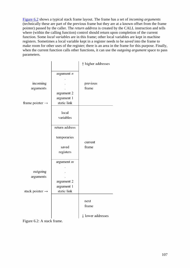
107

Figure 6.2 shows a typical stack frame layout. The frame has a set of incoming arguments (technically these are part of the previous frame but they are at a known offset from the frame pointer) passed by the caller. The return address is created by the CALL instruction and tells where (within the calling function) control should return upon completion of the current function. Some local variables are in this frame; other local variables are kept in machine registers. Sometimes a local variable kept in a register needs to be saved into the frame to make room for other uses of the register; there is an area in the frame for this purpose. Finally, when the current function calls other functions, it can use the outgoing argument space to pass parameters.

Figure 6.2: A stack frame.

108

THE FRAME POINTER

Suppose a function g(…) calls the function f(a1,…, an). We say g is the caller and f is the callee. On entry to f, the stack pointer points to the first argument that g passes to f . On entry, f allocates a frame by simply subtracting the frame size from the stack pointer SP.

The old SP becomes the current frame pointer FP. In some frame layouts, FP is a separate register; the old value of FP is saved in memory (in the frame) and the new FP becomes the old SP. When f exits, it just copies FP back to SP and fetches back the saved FP. This arrangement is useful if f 's frame size can vary, or if frames are not always contiguous on the stack. But if the frame size is fixed, then for each function f the FP will always differ from SP by a known constant, and it is not necessary to use a register for FP at all − FP is a "fictional" register whose value is always SP + framesize.

Why talk about a frame pointer at all? Why not just refer to all variables, parameters, etc., by their offset from SP, if the frame size is constant? The frame size is not known until quite late in the compilation process, when the number of memory-resident temporaries and saved registers is determined. But it is useful to know the offsets of formal parameters and local variables much earlier. So, for convenience, we still talk about a frame pointer. And we put the formals and locals right near the frame pointer at offsets that are known early; the temporaries and saved registers go farther away, at offsets that are known later.

REGISTERS

A modern machine has a large set of registers (typically 32 of them). To make compiled programs run fast, it's useful to keep local variables, intermediate results of expressions, and other values in registers instead of in the stack frame. Registers can be directly accessed by arithmetic instructions; on most machines, accessing memory requires separate load and store instructions. Even on machines whose arithmetic instructions can access memory, it is faster to access registers.

A machine (usually) has only one set of registers, but many different procedures and functions need to use registers. Suppose a function f is using register r to hold a local variable and calls procedure g, which also uses r for its own calculations. Then r must be saved (stored into a stack frame) before g uses it and restored (fetched back from the frame) after g is finished using it. But is it f 's responsibility to save and restore the register, or g's? We say that r is a caller-save register if the caller (in this case, f) must save and restore the register, and r is callee-save if it is the responsibility of the callee (in this case, g).

On most machine architectures, the notion of caller-save or callee-save register is not something built into the hardware, but is a convention described in the machine's reference manual. On the MIPS computer, for example, registers 16-23 are preserved across procedure calls (callee-save), and all other registers are not preserved across procedure calls (caller-save).

Sometimes the saves and restores are unnecessary. If f knows that the value of some variable x will not be needed after the call, it may put x in a caller-save register and not save it when calling g. Conversely, if f hasalocal variable i that is needed before and after several function calls, it may put i in some callee-save register ri, andsave ri just once (upon entry to f )and fetch it back just once (before returning from f ). Thus, the wise selection of a caller-save or callee-save register for each local variable and temporary can reduce the number of stores and

109

fetches a program executes. We will rely on our register allocator to choose the appropriate kind of register for each local variable and temporary value.

PARAMETER PASSING

On most machines whose calling conventions were designed in the 1970s, function arguments were passed on the stack.[1] But this causes needless memory traffic. Studies of actual programs have shown that very few functions have more than four arguments, and almost none have more than six. Therefore, parameter-passing conventions for modern machines specify that the first k arguments (for k = 4 or k = 6, typically) of a function are passed in registers rp, …, rp+ k−1, and the rest of the arguments are passed in memory.

Now, suppose f(a1, …, an) (which received its parameters in r1, …, rn, for example) calls h(z). It must pass the argument z in r1; so f saves the old contents of r1 (the value a1) in its stack frame before calling h. But there is the memory traffic that was supposedly avoided by passing arguments in registers! How has the use of registers saved any time?

There are four answers, any or all of which can be used at the same time:

1. Some procedures don't call other procedures - these are called leaf procedures. What proportion of procedures are leaves? Well, if we make the (optimistic) assumption that the average procedure calls either no other procedures or calls at least two others, then we can describe a "tree" of procedure calls in which there are more leaves than internal nodes. This means that most procedures called are leaf procedures.

Leaf procedures need not write their incoming arguments to memory. In fact, often they don't need to allocate a stack frame at all. This is an important savings.

2. Some optimizing compilers use interprocedural register allocation, analyzing all the functions in an entire program at once. Then they assign different procedures different registers in which to receive parameters and hold local variables. Thus f(x) might receive x in r1, but call h(z) with z in r7.

3. Even if f is not a leaf procedure, it might be finished with all its use of the argument x by the time it calls h (technically, x is a dead variable at the point where h is called). Then f can overwrite r1 without saving it.

4. Some architectures have register windows, so that each function invocation can allocate a fresh set of registers without memory traffic.

If f needs to write an incoming parameter into the frame, where in the frame should it go? Ideally, f 's frame layout should matter only in the implementation of f . A straightforward approach would be for the caller to pass arguments a1, …; ak in registers and ak+1, …; an at the end of its own frame - the place marked outgoing arguments in Figure 6.2 - which become the incoming arguments of the callee. If the callee needed to write any of these arguments to memory, it would write them to the area marked local variables.

The C programming language actually allows you to take the address of a formal parameter and guarantees that all the formal parameters of a function are at consecutive addresses! This is the varargs feature that printf uses. Allowing programmers to take the address of a parameter can lead to a dangling reference if the address outlives the frame - as the address of x will in int *f(int x){return &x;} - and even when it does not lead to bugs, the consecutive-address rule for parameters constrains the compiler and makes stack-frame layout

110

more complicated. To resolve the contradiction that parameters are passed in registers, but have addresses too, the first k parameters are passed in registers; but any parameter whose address is taken must be written to a memory location on entry to the function. To satisfy printf, the memory locations into which register arguments are written must all be consecutive with the memory locations in which arguments k + 1, k + 2, etc., are written. Therefore, C programs can't have some of the arguments saved in one place and some saved in another - they must all be saved contiguously.

So in the standard calling convention of many modern machines the calling function reserves space for the register arguments in its own frame, next to the place where it writes argument k + 1. But the calling function does not actually write anything there; that space is written into by the called function, and only if the called function needs to write arguments into memory for any reason.

A more dignified way to take the address of a local variable is to use call-by-reference. With call-by-reference, the programmer does not explicitly manipulate the address of a variable x. Instead, if x is passed as the argument to f(y), where y is a "by-reference" parameter, the compiler generates code to pass the address of x instead of the contents of x. At any use of y within the function, the compiler generates an extra pointer dereference. With call-by-reference, there can be no "dangling reference", since y must disappear when f returns, and f returns before x's scope ends.

RETURN ADDRESSES

When function g calls function f, eventually f must return. It needs to know where to go back to. If the call instruction within g is at address a, then (usually) the right place to return to is a + 1, the next instruction in g. This is called the return address.

On 1970s machines, the return address was pushed on the stack by the call instruction. Modern science has shown that it is faster and more flexible to pass the return address in a register, avoiding memory traffic and also avoiding the need to build any particular stack discipline into the hardware.

On modern machines, the call instruction merely puts the return address (the address of the instruction after the call) in a designated register. A nonleaf procedure will then have to write it to the stack (unless interprocedural register allocation is used), but a leaf procedure will not.

FRAME-RESIDENT VARIABLES

So a modern procedure-call convention will pass function parameters in registers, pass the return address in a register, and return the function result in a register. Many of the local variables will be allocated to registers, as will the intermediate results of expression evaluation. Values are written to memory (in the stack frame) only when necessary for one of these reasons:

• the variable will be passed by reference, so it must have a memory address (or, in the C language the & operator is anywhere applied to the variable);

• the variable is accessed by a procedure nested inside the current one;[2] • the value is too big to fit into a single register;[3] • the variable is an array, for which address arithmetic is necessary to extract

components;

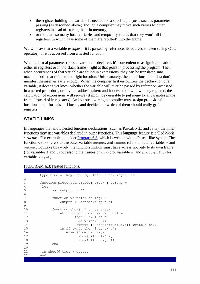
111

• the register holding the variable is needed for a specific purpose, such as parameter passing (as described above), though a compiler may move such values to other registers instead of storing them in memory;

• or there are so many local variables and temporary values that they won't all fit in registers, in which case some of them are "spilled" into the frame.

We will say that a variable escapes if it is passed by reference, its address is taken (using C's & operator), or it is accessed from a nested function.

When a formal parameter or local variable is declared, it's convenient to assign it a location - either in registers or in the stack frame - right at that point in processing the program. Then, when occurrences of that variable are found in expressions, they can be translated into machine code that refers to the right location. Unfortunately, the conditions in our list don't manifest themselves early enough. When the compiler first encounters the declaration of a variable, it doesn't yet know whether the variable will ever be passed by reference, accessed in a nested procedure, or have its address taken; and it doesn't know how many registers the calculation of expressions will require (it might be desirable to put some local variables in the frame instead of in registers). An industrial-strength compiler must assign provisional locations to all formals and locals, and decide later which of them should really go in registers.

STATIC LINKS

In languages that allow nested function declarations (such as Pascal, ML, and Java), the inner functions may use variables declared in outer functions. This language feature is called block structure. For example, consider Program 6.3, which is written with a Pascal-like syntax. The function write refers to the outer variable output, and indent refers to outer variables n and output. To make this work, the function indent must have access not only to its own frame (for variables i and s) but also to the frames of show (for variable n) and prettyprint (for variable output).

PROGRAM 6.3: Nested functions. 1 type tree = {key: string, left: tree, right: tree} 2 3 function prettyprint(tree: tree) : string = 4 let 5 var output := "" 6 7 function write(s: string) = 8 output := concat(output,s) 9 10 function show(n:int, t: tree) = 11 let function indent(s: string) = 12 (for i := 1 to n 13 do write(" "); 14 output := concat(output,s); write("\n")) 15 in if t=nil then indent(".") 16 else (indent(t.key); 17 show(n+1,t.left); 18 show(n+1,t.right)) 19 end 20 21 in show(0,tree); output 22 end

112

There are several methods to accomplish this:

• Whenever a function f is called, it can be passed a pointer to the frame of the function statically enclosing f ; this pointer is the static link.

• A global array can be maintained, containing - in position i - a pointer to the frame of the most recently entered procedure whose static nesting depth is i. This array is called a display.

• When g calls f, each variable of g that is actually accessed by f (or by any function nested inside f ) is passed to f as an extra argument. This is called lambda lifting.

We will describe in detail only the method of static links. Which method should be used in practice? See Exercise 6.6.

Whenever a function f is called, it is passed a pointer to the stack frame of the "current" (most recently entered) activation of the function g that immediately encloses f in the text of the program.

For example, in Program 6.3:

Line#

21 prettyprint calls show, passing prettyprint's own frame pointer as show's static link.

10 show stores its static link (the address of prettyprint's frame) into its own frame.

15 show calls indent, passing its own frame pointer as indent's static link.

17 show calls show, passing its own static link (not its own frame pointer) as the static link.

12 indent uses the value n from show's frame. To do so, it fetches at an appropriate offset from indent's static link (which points at the frame of show).

13 indent calls write. It must pass the frame pointer of prettyprint as the static link. To obtain this, it first fetches at an offset from its own static link (from show's frame), the static link that had been passed to show.

14 indent uses the variable output from prettyprint'sframe.Todosoit starts with its own static link, then fetches show's, then fetches output.[4]

So on each procedure call or variable access, a chain of zero or more fetches is required; the length of the chain is just the difference in static nesting depth between the two functions involved.

6.2 FRAMES IN THE MiniJava COMPILER

What sort of stack frames should the MiniJava compiler use? Here we face the fact that every target-machine architecture will have a different standard stack frame layout. If we want MiniJava functions to be able to call C functions, we should use the standard layout. But we don't want the specifics of any particular machine intruding on the implementation of the translation module of the MiniJava compiler.

113

Thus we must use abstraction. Just as the Symbol module provides a clean interface, and hides the internal representation of Symbol.Table from its clients, we must use an abstract representation for frames.

The frame interface will look something like this:

package Frame; import Temp.Temp; import Temp.Label; public abstract class Access { ... } public abstract class AccessList {...head;...tail;... } public abstract class Frame { abstract public Frame newFrame(Label name, Util.BoolList formals); public Label name; public AccessList formals; abstract public Access allocLocal(boolean escape); /* ... other stuff, eventually ... * }

The abstract class Frame is implemented by a module specific to the target machine. For example, if compiling to the MIPS architecture, there would be

package Mips; class Frame extends Frame.Frame { ... }

In general, we may assume that the machine-independent parts of the compiler have access to this implementation of Frame; for example,

// in class Main.Main: Frame.Frame frame = new Mips.Frame(...);

In this way the rest of the compiler may access frame without knowing the identity of the target machine (except an occurrence of the word Mips here and there).

The class Frame holds information about formal parameters and local variables allocated in this frame. To make a new frame for a function f with k formal parameters, call newFrame(f, l), where l is a list of k booleans: true for each parameter that escapes and false for each parameter that does not. (In MiniJava, no parameters ever escape.) The result will be a Frame object. For example, consider a three-argument function named g whose first argument escapes (needs to be kept in memory). Then

frame.newFrame(g,new BoolList(true, new BoolList(false, new BoolList(false, null))))

returns a new frame object.

The Access class describes formals and locals that may be in the frame or in registers. This is an abstract data type, so its implementation as a pair of subclasses is visible only inside the Frame module:

package Mips; class InFrame extends Frame.Access {int offset; ... } class InReg extends Frame.Access {Temp temp; ... }

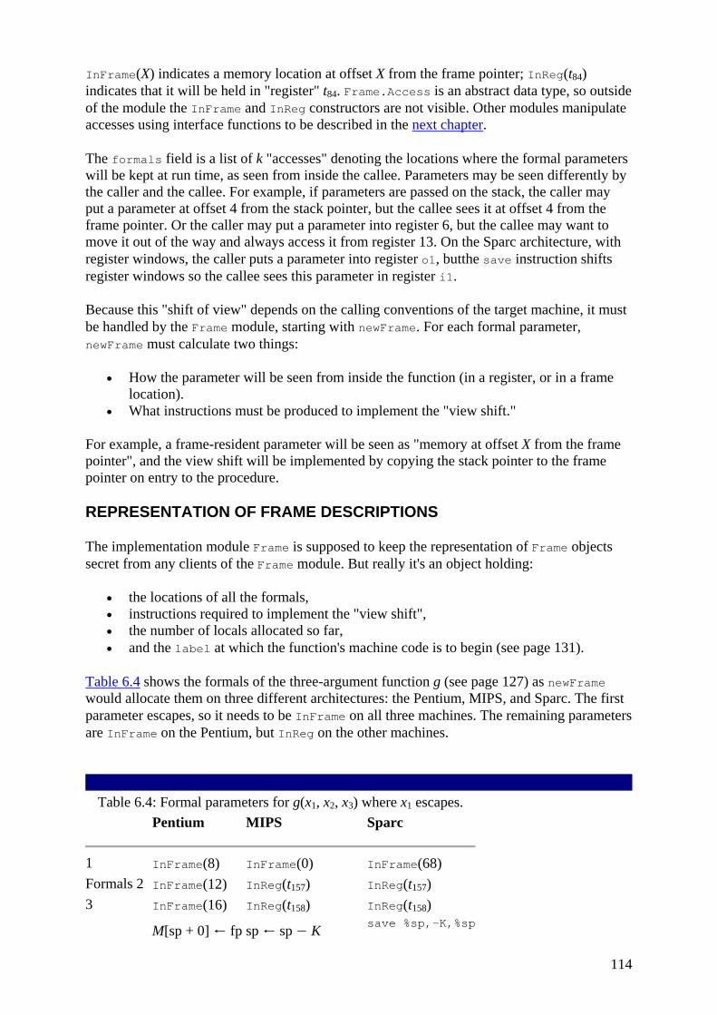
114

InFrame(X) indicates a memory location at offset X from the frame pointer; InReg(t84) indicates that it will be held in "register" t84. Frame.Access is an abstract data type, so outside of the module the InFrame and InReg constructors are not visible. Other modules manipulate accesses using interface functions to be described in the next chapter.

The formals field is a list of k "accesses" denoting the locations where the formal parameters will be kept at run time, as seen from inside the callee. Parameters may be seen differently by the caller and the callee. For example, if parameters are passed on the stack, the caller may put a parameter at offset 4 from the stack pointer, but the callee sees it at offset 4 from the frame pointer. Or the caller may put a parameter into register 6, but the callee may want to move it out of the way and always access it from register 13. On the Sparc architecture, with register windows, the caller puts a parameter into register o1, butthe save instruction shifts register windows so the callee sees this parameter in register i1.

Because this "shift of view" depends on the calling conventions of the target machine, it must be handled by the Frame module, starting with newFrame. For each formal parameter, newFrame must calculate two things:

• How the parameter will be seen from inside the function (in a register, or in a frame location).

• What instructions must be produced to implement the "view shift."

For example, a frame-resident parameter will be seen as "memory at offset X from the frame pointer", and the view shift will be implemented by copying the stack pointer to the frame pointer on entry to the procedure.

REPRESENTATION OF FRAME DESCRIPTIONS

The implementation module Frame is supposed to keep the representation of Frame objects secret from any clients of the Frame module. But really it's an object holding:

• the locations of all the formals, • instructions required to implement the "view shift", • the number of locals allocated so far, • and the label at which the function's machine code is to begin (see page 131).

Table 6.4 shows the formals of the three-argument function g (see page 127) as newFrame would allocate them on three different architectures: the Pentium, MIPS, and Sparc. The first parameter escapes, so it needs to be InFrame on all three machines. The remaining parameters are InFrame on the Pentium, but InReg on the other machines.

Table 6.4: Formal parameters for g(x1, x2, x3) where x1 escapes. Pentium MIPS Sparc

1 InFrame(8) InFrame(0) InFrame(68) Formals 2 InFrame(12) InReg(t157) InReg(t157) 3 InFrame(16) InReg(t158) InReg(t158) M[sp + 0] ← fp sp ← sp − K save %sp,-K,%sp

115

Table 6.4: Formal parameters for g(x1, x2, x3) where x1 escapes. Pentium MIPS Sparc

View Shift fp ← sp M[sp + K + 0] ← r4 M[fp + 68] ← i0 sp ← sp − K t157 ← r5 t157 ← i1 t158 ← r6 t158 ← i2

The freshly created temporaries t157 and t158, and the move instructions that copy r4 and r5 into them (or on the Sparc, i1 and i2), may seem superfluous. Why shouldn't the body of g just access these formals directly from the registers in which they arrive? To see why not, consider

void m(int x, int y) { h(y,y); h(x,x); }

If x stays in "parameter register 1" throughout m, and y is passed to h in parameter register 1, then there is a problem.

The register allocator will eventually choose which machine register should hold t157. If there is no interference of the type shown in function m, then (on the MIPS) the allocator will take care to choose register r4 to hold t157 and r5 to hold t158. Then the move instructions will be unnecessary and will be deleted at that time.

See also pages 157 and 251 for more discussion of the view shift.

LOCAL VARIABLES

Some local variables are kept in the frame; others are kept in registers. To allocate a new local variable in a frame f, the translation phase calls

f.allocLocal(false)

This returns an InFrame access with an offset from the frame pointer. For example, to allocate two local variables on the Sparc, allocLocal would be called twice, returning successively InFrame(-4) and InFrame(-8), which are standard Sparc frame-pointer offsets for local variables.

The boolean argument to allocLocal specifies whether the new variable escapes and needs to go in the frame; if it is false, then the variable can be allocated in a register. Thus, f.allocLocal(false) might create InReg(t481).

For MiniJava, that no variables escape. This is because in MiniJava:

• there is no nesting of classes and methods; • it is not possible to take the address of a variable; • integers and booleans are passed by value; and • objects, including integer arrays, can be represented as pointers that are also

passedbyvalue.

116

The calls to allocLocal need not come immediately after the frame is created. In many languages, there may be variable-declaration blocks nested inside the body of a function. For example,

void f() {int v=6; print(v); {int v=7; print(v); } print(v); {int v=8; print(v); } print(v); }

In this case there are three different variables v. The program will print the sequence 6 7 6 8 6. As each variable declaration is encountered in processing the program, we will allocate a temporary or new space in the frame, associated with the name v. As each end (or closing brace) is encountered, the association with v will be forgotten - but the space is still reserved in the frame. Thus, there will be a distinct temporary or frame slot for every variable declared within the entire function.

The register allocator will use as few registers as possible to represent the temporaries. In this example, the second and third v variables (initialized to 7 and 8) could be held in the same register. A clever compiler might also optimize the size of the frame by noticing when two frame-resident variables could be allocated to the same slot.

TEMPORARIES AND LABELS

The compiler's translation phase will want to choose registers for parameters and local variables, and choose machine-code addresses for procedure bodies. But it is too early to determine exactly which registers are available, or exactly where a procedure body will be located. We use the word temporary to mean a value that is temporarily held in a register, and the word label to mean some machine-language location whose exact address is yet to be determined - just like a label in assembly language.

Temps are abstract names for local variables; labels are abstract names for static memory addresses. The Temp module manages these two distinct sets of names.

package Temp; public class Temp { public String toString(); public Temp(); } public class Label { public String toString(); public Label(); public Label(String s); public Label(Symbol s); } public class TempList {...} public class LabelList {...}

117

new Temp.Temp() returns a new temporary from an infinite set of temps. new Temp.Label() returns a new label from an infinite set of labels. And new Temp.Label(string)) returns a new label whose assembly-language name is string.

When processing the declaration m(…), a label for the address of m's machine code can be produced by new Temp.Label(). It's tempting to call new Temp.Label("m") instead - the assembly-language program will be easier to debug if it uses the label m instead of L213 - but unfortunately there could be two different methods named m in different classes. A better idea is to call new Temp.Label("C"+"$"+"m"), where C is the name of the class in which the method m occurs.

MANAGING STATIC LINKS

The Frame module should be independent of the specific source language being compiled. Many source languages, including MiniJava, do not have nested function declarations; thus, Frame should not know anything about static links. Instead, this is the responsibility of the translation phase. The translation phase would know that each frame contains a static link. The static link would be passed to a function in a register and stored into the frame. Since the static link behaves so much like a formal parameter, we can treat it as one (as much as possible).

[1]Before about 1960, they were passed not on the stack but in statically allocated blocks of memory, which precluded the use of recursive functions.

[2]However, with register allocation across function boundaries, local variables accessed by inner functions can sometimes go in registers, as long as the inner function knows where to look.

[3]However, some compilers spread out a large value into several registers for efficiency.

[4]This program would be cleaner if show called write here instead of manipulating output directly, but it would not be as instructive.

PROGRAM FRAMES

If you are compiling for the Sparc, implement the Sparc package containing Sparc/SparcFrame.java. If compiling for the MIPS, implement the Mips package, and so on.

If you are working on a RISC machine (such as MIPS or Sparc) that passes the first k parameters in registers and the rest in memory, keep things simple by handling only the case where there are k or fewer parameters.

Supporting files available in $MINIJAVA/chap6 include:

Temp/* The module supporting temporaries and labels.

Util/BoolList.java The class for lists of booleans.

Optional: Handle functions with more than k formal parameters.

118

FURTHER READING

The use of a single contiguous stack to hold variables and return addresses dates from Lisp [McCarthy 1960] and Algol [Naur et al. 1963]. Block structure (the nesting of functions) and the use of static links are also from Algol.

Computers and compilers of the 1960s and '70s kept most program variables in memory, so that there was less need to worry about which variables escaped (needed addresses). The VAX, built in 1978, had a procedure-call instruction that assumed all arguments were pushed on the stack, and itself pushed program counter, frame pointer, argument pointer, argument count, and callee-save register mask on the stack [Leonard 1987].

With the RISC revolution [Patterson 1985] came the idea that procedure calling can be done with much less memory traffic. Local variables should be kept in registers by default; storing and fetching should be done as needed, driven by "spilling" in the register allocator [Chaitin 1982].

Most procedures don't have more than five arguments and five local variables [Tanenbaum 1978]. To take advantage of this, Chow et al. [1986] and Hopkins [1986] designed calling conventions optimized for the common case: The first four arguments are passed in registers, with the (rare) extra arguments passed in memory; compilers use both caller- and callee-save registers for local variables; leaf procedures don't even need stack frames of their own if they can operate within the caller-save registers; and even the return address need not always be pushed on the stack.

EXERCISES

• 6.1 Using the C compiler of your choice (or a compiler for another language), compile some small test functions into assembly language. On Unix this is usually done by cc -S. Turn on all possible compiler optimizations. Then evaluate the compiled programs by these criteria:

a. a. Are local variables kept in registers? b. b. If local variable b is live across more than one procedure call, is it kept in a

callee-save register? Explain how doing this would speed up the following program:

c. int f(int a) {int b; b=a+1; g(); h(b); return b+2;} d. c. If local variable x is never live across a procedure call, is it properly kept in a

caller-save register? Explain how doing this would speed up the following program:

e. void h(int y) {int x; x=y+1; f(y); f(2);} • 6.2 If you have a C compiler that passes parameters in registers, make it generate

assembly language for this function: • extern void h(int, int); • void m(int x, int y) {h(y,y); h(x,x);}

Clearly, if arguments to m(x, y) arrive in registers rarg1 and rarg2, and arguments to h must be passed in rarg1 and rarg2, then x cannot stay in rarg1 during the marshalling of arguments to h(y, y). Explain when and how your C compiler moves x out of the rarg1 register so as to call h(y, y).

• 6.3 For each of the variables a, b, c, d, e in this C program, say whether the variable should be kept in memory or a register, and why.

• int f(int a, int b)

119

• { int c[3], d, e; • d=a+1; • e=g(c, &b); • return e+c[1]+b; • } • *6.4 How much memory should this program use? • int f(int i) {int j,k; j=i*i; k=i?f(i-1):0; return k+j;} • void main() {f(100000);}

a. Imagine a compiler that passes parameters in registers, wastes no space providing "backup storage" for parameters passed in registers, does not use static links, and in general makes stack frames as small as possible. How big should each stack frame for f be, in words?

b. What is the maximum memory use of this program, with such a compiler? c. Using your favorite C compiler, compile this program to assembly language

and report the size of f 's stack frame. d. Calculate the total memory use of this program with the real C compiler. e. Quantitatively and comprehensively explain the discrepancy between (a) and

(c). f. Comment on the likelihood that the designers of this C compiler considered

deeply recursive functions important in real programs. • *6.5 Instead of (or in addition to) using static links, there are other ways of getting

access to nonlocal variables. One way is just to leave the variable in a register! • function f() : int = • let var a := 5 • function g() : int = • (a+1) • in g()+g() • end

If a is left in register r7 (for example) while g is called, then g can just access it from there.

What properties must a local variable, the function in which it is defined, and the functions in which it is used, have for this trick to work?

• *6.6 A display is a data structure that may be used as an alternative to static links for maintaining access to nonlocal variables. It is an array of frame pointers, indexed by static nesting depth. Element Di of the display always points to the most recently called function whose static nesting depth is i.

The bookkeeping performed by a function f, whose static nesting depth is i, looks like:

Copy Di to save locationin stack frame Copy frame pointer to Di ... body of f ... Copy save locationback to Di

In Program 6.3, function prettyprint is at depth 1, write and show are at depth 2, and so on.

a. Show the sequence of machine instructions required to fetch the variable output into a register at line 14 of Program 6.3, using static links.

b. Show the machine instructions required if a display were used instead.

120

c. When variable x is declared at depth d1 and accessed at depth d2, how many instructions does the static-link method require to fetch x?

d. How many does the display method require? e. How many instructions does static-link maintenance require for a procedure

entry and exit (combined)? f. How many instructions does display maintenance require for procedure entry

and exit?

Should we use displays instead of static links? Perhaps; but the issue is more complicated. For languages such as Pascal with block structure but no function variables, displays work well.

But the full expressive power of block structure is obtained when functions can be returned as results of other functions, as in Scheme and ML. For such languages, there are more issues to consider than just variable-access time and procedure entry-exit cost: there is closure-building cost, and the problem of avoiding useless data kept live in closures. Chapter 15 explains some of the issues.

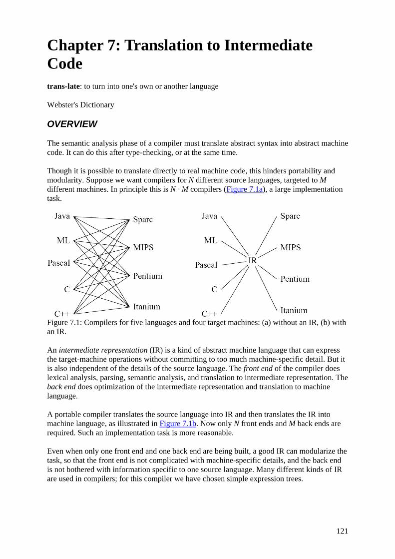
121

Chapter 7: Translation to Intermediate Code trans-late: to turn into one's own or another language


OVERVIEW

The semantic analysis phase of a compiler must translate abstract syntax into abstract machine code. It can do this after type-checking, or at the same time.

Though it is possible to translate directly to real machine code, this hinders portability and modularity. Suppose we want compilers for N different source languages, targeted to M different machines. In principle this is N · M compilers (Figure 7.1a), a large implementation task.

Figure 7.1: Compilers for five languages and four target machines: (a) without an IR, (b) with an IR.

An intermediate representation (IR) is a kind of abstract machine language that can express the target-machine operations without committing to too much machine-specific detail. But it is also independent of the details of the source language. The front end of the compiler does lexical analysis, parsing, semantic analysis, and translation to intermediate representation. The back end does optimization of the intermediate representation and translation to machine language.

A portable compiler translates the source language into IR and then translates the IR into machine language, as illustrated in Figure 7.1b. Now only N front ends and M back ends are required. Such an implementation task is more reasonable.

Even when only one front end and one back end are being built, a good IR can modularize the task, so that the front end is not complicated with machine-specific details, and the back end is not bothered with information specific to one source language. Many different kinds of IR are used in compilers; for this compiler we have chosen simple expression trees.

122

7.1 INTERMEDIATE REPRESENTATION TREES

The intermediate representation tree language is defined by the package Tree, containing abstract classes Stm and Exp and their subclasses, as shown in Figure 7.2.

package Tree; abstract class Exp CONST(int value) NAME(Label label) TEMP(Temp.Temp temp) BINOP(int binop, Exp left, Exp right) MEM(Exp exp) CALL(Exp func, ExpList args) ESEQ(Stm stm, Exp exp) abstract class Stm MOVE(Exp dst, Exp src) EXP(Exp exp) JUMP(Exp exp, Temp.LabelList targets) CJUMP(int relop, Exp left, Exp right, Label iftrue, Label iffalse) SEQ(Stm left, Stm right) LABEL(Label label) other classes: ExpList(Exp head, ExpList tail) StmList(Stm head, StmList tail) other constants: final static int BINOP.PLUS, BINOP.MINUS, BINOP.MUL, BINOP.DIV, BINOP.AND, BINOP.OR, BINOP.LSHIFT, BINOP.RSHIFT, BINOP.ARSHIFT, BINOP.XOR; final static int CJUMP.EQ, CJUMP.NE, CJUMP.LT, CJUMP.GT, CJUMP.LE, CJUMP.GE, CJUMP.ULT, CJUMP.ULE, CJUMP.UGT, CJUMP.UGE;

Figure 7.2: Intermediate representation trees.

A good intermediate representation has several qualities:

• It must be convenient for the semantic analysis phase to produce. ∊ It must be convenient to translate into real machine language, for all the desired target machines.

• Each construct must have a clear and simple meaning, so that optimizing transformations that rewrite the intermediate representation can easily be specified and implemented.

Individual pieces of abstract syntax can be complicated things, such as array subscripts, procedure calls, and so on. And individual "real machine" instructions can also have a complicated effect (though this is less true of modern RISC machines than of earlier architectures). Unfortunately, it is not always the case that complex pieces of the abstract syntax correspond exactly to the complex instructions that a machine can execute.

Therefore, the intermediate representation should have individual components that describe only extremely simple things: a single fetch, store, add, move, or jump. Then any "chunky" piece of abstract syntax can be translated into just the right set of abstract machine

123

instructions; and groups of abstract machine instructions can be clumped together (perhaps in quite different clumps) to form "real" machine instructions.

Here is a description of the meaning of each tree operator. First, the expressions (Exp), which stand for the computation of some value (possibly with side effects):

• CONST(i) The integer constant i. • NAME(n) The symbolic constant n (corresponding to an assembly language label). • TEMP(t) Temporary t. A temporary in the abstract machine is similar to a register in a

real machine. However, the abstract machine has an infinite number of temporaries. • BINOP(o, e1, e2) The application of binary operator o to operands e1, e2.

Subexpression e1 is evaluated before e2. The integer arithmetic operators are PLUS, MINUS, MUL, DIV; the integer bitwise logical operators are AND, OR, XOR; the integer logical shift operators are LSHIFT, RSHIFT; the integer arithmetic right-shift is ARSHIFT. The MiniJava language has only one logical operator, but the intermediate language is meant to be independent of any source language; also, the logical operators might be used in implementing other features of MiniJava.

• MEM(e) The contents of wordSize bytes of memory starting at address e (where wordSize is defined in the Frame module). Note that when MEM is used as the left child of a MOVE, it means "store", but anywhere else it means "fetch."

• CALL(f, l) A procedure call: the application of function f to argument list l. The subexpression f is evaluated before the arguments which are evaluated left to right.

• ESEQ(s, e) The statement s is evaluated for side effects, then e is evaluated for a result.

The statements (stm) of the tree language perform side effects and control flow:

• MOVE(TEMP t, e) Evaluate e and move it into temporary t. • MOVE(MEM(e1) e2) Evaluate e1, yielding address a. The nevaluate e2, and store the

result into wordSize bytes of memory starting at a. • EXP(e) Evaluate e and discard the result. • JUMP(e, labs) Transfer control (jump) to address e. The destination e may be a literal

label, as in NAME(lab), or it may be an address calculated by any other kind of expression. For example, a C-language switch(i) statement may be implemented by doing arithmetic on i. The list of labels labs specifies all the possible locations that the expression e can evaluate to; this is necessary for dataflow analysis later. The common case of jumping to a known label l is written as JUMP(NAME l, new LabelList(l, null)), but the JUMP class has an extra constructor so that this can be abbreviated as JUMP(l).

• CJUMP(o, e1, e2, t, f) Evaluate e1, e2 in that order, yielding values a, b. Then compare a, b using the relational operator o. If the result is true, jump to t; otherwise jump to f . The relational operators are EQ and NE for integer equality and nonequality (signed or unsigned); signed integer inequalities LT, GT, LE, GE; and unsigned integer inequalities ULT, ULE, UGT, UGE.

• SEQ(s1, s2) The statement s1 followed by s2. • LABEL(n) Define the constant value of name n to be the current machine code

address. This is like a label definition in assembly language. The value NAME(n) may be the target of jumps, calls, etc.

It is almost possible to give a formal semantics to the Tree language. However, there is no provision in this language for procedure and function definitions - we can specify only the

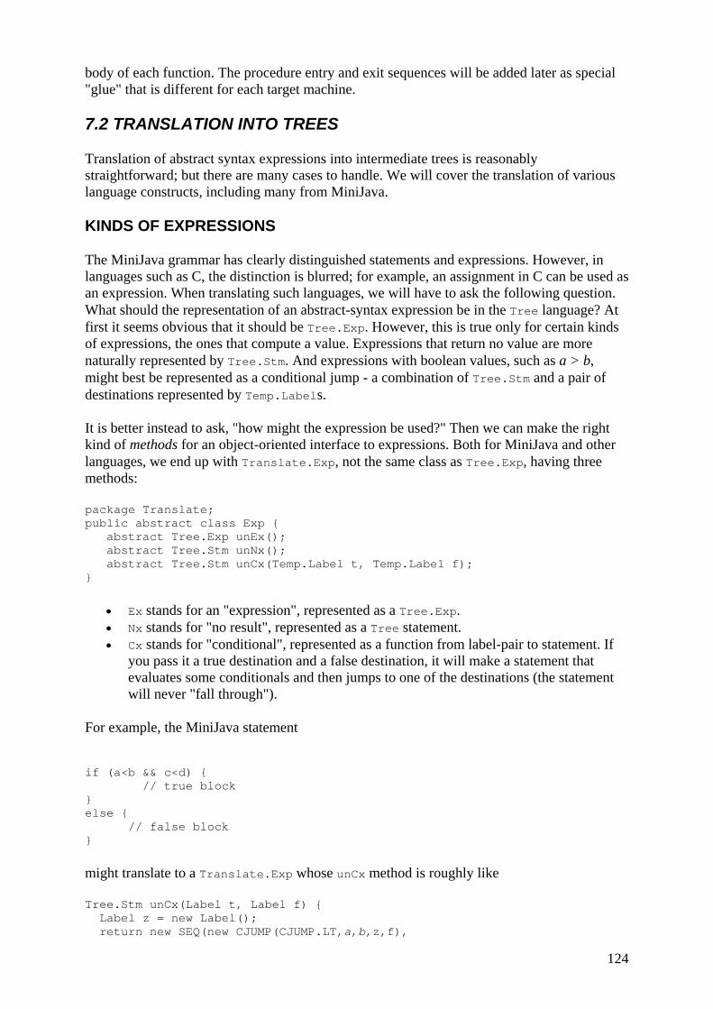
124

body of each function. The procedure entry and exit sequences will be added later as special "glue" that is different for each target machine.

7.2 TRANSLATION INTO TREES

Translation of abstract syntax expressions into intermediate trees is reasonably straightforward; but there are many cases to handle. We will cover the translation of various language constructs, including many from MiniJava.

KINDS OF EXPRESSIONS

The MiniJava grammar has clearly distinguished statements and expressions. However, in languages such as C, the distinction is blurred; for example, an assignment in C can be used as an expression. When translating such languages, we will have to ask the following question. What should the representation of an abstract-syntax expression be in the Tree language? At first it seems obvious that it should be Tree.Exp. However, this is true only for certain kinds of expressions, the ones that compute a value. Expressions that return no value are more naturally represented by Tree.Stm. And expressions with boolean values, such as a > b, might best be represented as a conditional jump - a combination of Tree.Stm and a pair of destinations represented by Temp.Labels.

It is better instead to ask, "how might the expression be used?" Then we can make the right kind of methods for an object-oriented interface to expressions. Both for MiniJava and other languages, we end up with Translate.Exp, not the same class as Tree.Exp, having three methods:

package Translate; public abstract class Exp { abstract Tree.Exp unEx(); abstract Tree.Stm unNx(); abstract Tree.Stm unCx(Temp.Label t, Temp.Label f); }

• Ex stands for an "expression", represented as a Tree.Exp. • Nx stands for "no result", represented as a Tree statement. • Cx stands for "conditional", represented as a function from label-pair to statement. If

you pass it a true destination and a false destination, it will make a statement that evaluates some conditionals and then jumps to one of the destinations (the statement will never "fall through").

For example, the MiniJava statement

if (a<b && c<d) { // true block } else { // false block }

might translate to a Translate.Exp whose unCx method is roughly like

Tree.Stm unCx(Label t, Label f) { Label z = new Label(); return new SEQ(new CJUMP(CJUMP.LT,a,b,z,f),

125

new SEQ(new LABEL(z), new CJUMP(CJUMP.LT,c,d,t,f))); }

The abstract class Translate.Exp can be instantiated by several subclasses: Ex for an ordinary expression that yields a single value, Nx for an expression that yields no value, and Cx for a "conditional" expression that jumps to either t or f :

class Ex extends Exp { Tree.Exp exp; Ex(Tree.Exp e) {exp=e;} Tree.Exp unEx() {return exp;} Tree.Stm unNx() { ... ?... } Tree.Stm unCx(Label t, Label f) { ... ?... } } class Nx extends Exp { Tree.Stm stm; Nx(Tree.Stm s) {stm=s;} Tree.Exp unEx() { ... ?... } Tree.Stm unNx() {return stm;} Tree.Stm unCx(Label t, Label f) { ... ?... } }

But what does the unNx method of an Ex do? We have a simple Tree.Exp that yields a value, and we are asked to produce a Tree.Stm that produces no value. There is a conversion operator Tree.EXP, and unNx must apply it:

class Ex extends Exp { Tree.Exp exp;

⋮ Tree.Stm unNx() {return new Tree.EXP(exp); }

⋮ }

Each kind of Translate.Exp class must have similar conversion methods. For example, the MiniJava statement

flag = (a<b && c<d);

requires the unEx method of a Cx object so that a 1 (for true) or 0 (for false) can be stored into flag.

Program 7.3 shows the class Cx. The unEx method is of particular interest. To convert a "conditional" into a "value expression", we invent a new temporary r and new labels t and f. Then we make a Tree.Stm that moves the value 1 into r, and a conditional jump unCx(t, f) that implements the conditional. If the condition is false, then 0 is moved into r; if it is true, then execution proceeds at t and the second move is skipped. The result of the whole thing is just the temporary r containing zero or one.

PROGRAM 7.3: The Cx class. abstract class Cx extends Exp { Tree.Exp unEx() { Temp r = new Temp(); Label t = new Label(); Label f = new Label();

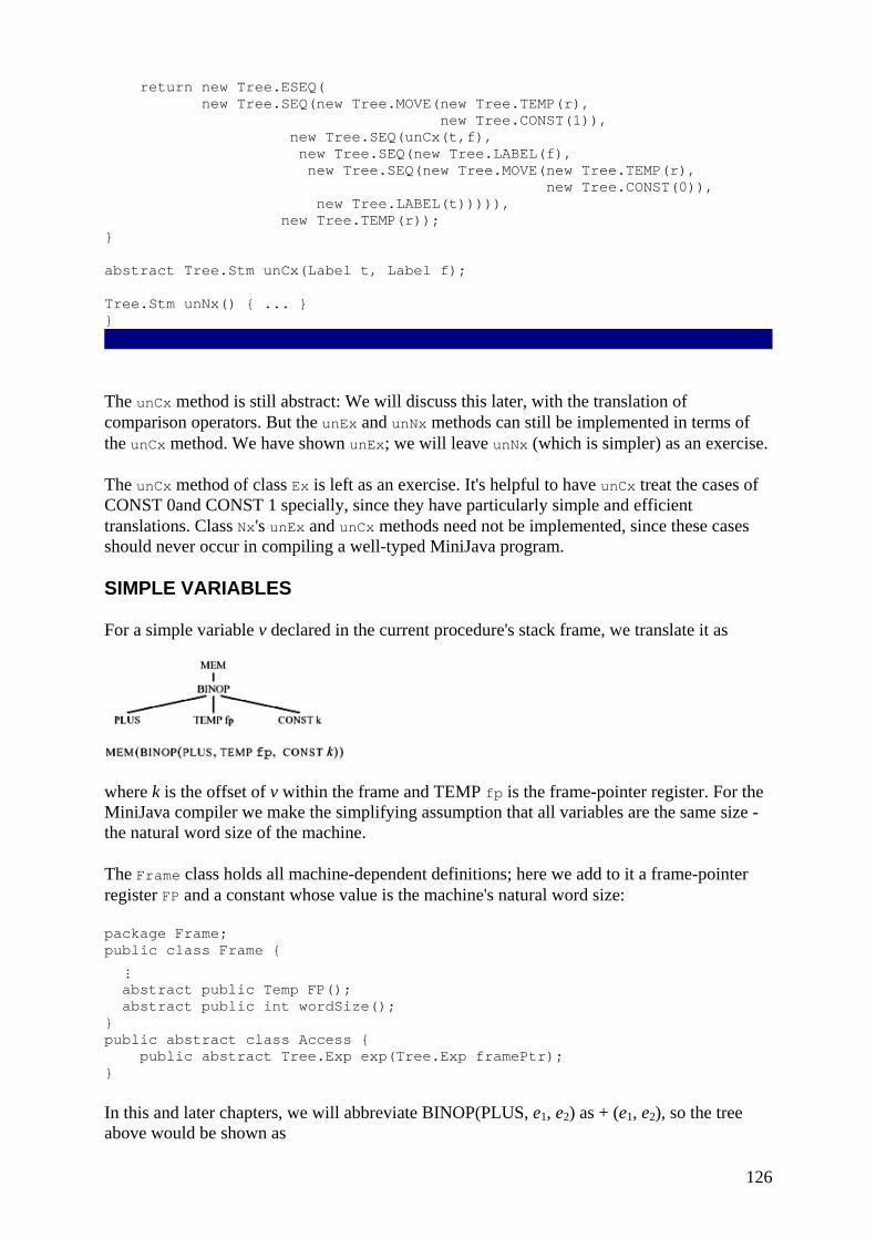
126

return new Tree.ESEQ( new Tree.SEQ(new Tree.MOVE(new Tree.TEMP(r), new Tree.CONST(1)), new Tree.SEQ(unCx(t,f), new Tree.SEQ(new Tree.LABEL(f), new Tree.SEQ(new Tree.MOVE(new Tree.TEMP(r), new Tree.CONST(0)), new Tree.LABEL(t))))), new Tree.TEMP(r)); } abstract Tree.Stm unCx(Label t, Label f); Tree.Stm unNx() { ... } }

The unCx method is still abstract: We will discuss this later, with the translation of comparison operators. But the unEx and unNx methods can still be implemented in terms of the unCx method. We have shown unEx; we will leave unNx (which is simpler) as an exercise.

The unCx method of class Ex is left as an exercise. It's helpful to have unCx treat the cases of CONST 0and CONST 1 specially, since they have particularly simple and efficient translations. Class Nx's unEx and unCx methods need not be implemented, since these cases should never occur in compiling a well-typed MiniJava program.

SIMPLE VARIABLES

For a simple variable v declared in the current procedure's stack frame, we translate it as

where k is the offset of v within the frame and TEMP fp is the frame-pointer register. For the MiniJava compiler we make the simplifying assumption that all variables are the same size - the natural word size of the machine.

The Frame class holds all machine-dependent definitions; here we add to it a frame-pointer register FP and a constant whose value is the machine's natural word size:

package Frame; public class Frame {

⋮ abstract public Temp FP(); abstract public int wordSize(); } public abstract class Access { public abstract Tree.Exp exp(Tree.Exp framePtr); }

In this and later chapters, we will abbreviate BINOP(PLUS, e1, e2) as + (e1, e2), so the tree above would be shown as

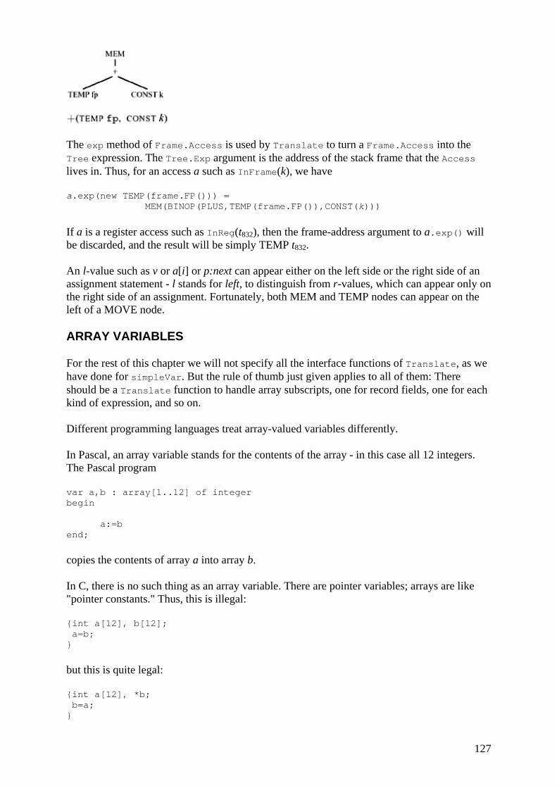
127

The exp method of Frame.Access is used by Translate to turn a Frame.Access into the Tree expression. The Tree.Exp argument is the address of the stack frame that the Access lives in. Thus, for an access a such as InFrame(k), we have

a.exp(new TEMP(frame.FP())) = MEM(BINOP(PLUS,TEMP(frame.FP()),CONST(k)))

If a is a register access such as InReg(t832), then the frame-address argument to a.exp() will be discarded, and the result will be simply TEMP t832.

An l-value such as v or a[i] or p:next can appear either on the left side or the right side of an assignment statement - l stands for left, to distinguish from r-values, which can appear only on the right side of an assignment. Fortunately, both MEM and TEMP nodes can appear on the left of a MOVE node.

ARRAY VARIABLES

For the rest of this chapter we will not specify all the interface functions of Translate, as we have done for simpleVar. But the rule of thumb just given applies to all of them: There should be a Translate function to handle array subscripts, one for record fields, one for each kind of expression, and so on.

Different programming languages treat array-valued variables differently.

In Pascal, an array variable stands for the contents of the array - in this case all 12 integers. The Pascal program

var a,b : array[1..12] of integer begin a:=b end;

copies the contents of array a into array b.

In C, there is no such thing as an array variable. There are pointer variables; arrays are like "pointer constants." Thus, this is illegal:

{int a[12], b[12]; a=b; }

but this is quite legal:

{int a[12], *b; b=a; }

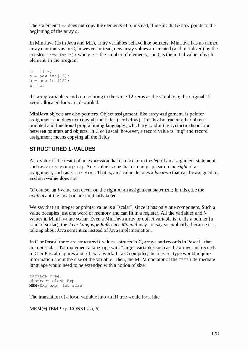
128

The statement b=a does not copy the elements of a; instead, it means that b now points to the beginning of the array a.

In MiniJava (as in Java and ML), array variables behave like pointers. MiniJava has no named array constants as in C, however. Instead, new array values are created (and initialized) by the construct new int[n]; where n is the number of elements, and 0 is the initial value of each element. In the program

int [] a; a = new int[12]; b = new int[12]; a = b;

the array variable a ends up pointing to the same 12 zeros as the variable b; the original 12 zeros allocated for a are discarded.

MiniJava objects are also pointers. Object assignment, like array assignment, is pointer assignment and does not copy all the fields (see below). This is also true of other object-oriented and functional programming languages, which try to blur the syntactic distinction between pointers and objects. In C or Pascal, however, a record value is "big" and record assignment means copying all the fields.

STRUCTURED L-VALUES

An l-value is the result of an expression that can occur on the left of an assignment statement, such as x or p.y or a[i+2]. An r-value is one that can only appear on the right of an assignment, such as a+3 or f(x). That is, an l-value denotes a location that can be assigned to, and an r-value does not.

Of course, an l-value can occur on the right of an assignment statement; in this case the contents of the location are implicitly taken.

We say that an integer or pointer value is a "scalar", since it has only one component. Such a value occupies just one word of memory and can fit in a register. All the variables and l-values in MiniJava are scalar. Even a MiniJava array or object variable is really a pointer (a kind of scalar); the Java Language Reference Manual may not say so explicitly, because it is talking about Java semantics instead of Java implementation.

In C or Pascal there are structured l-values - structs in C, arrays and records in Pascal - that are not scalar. To implement a language with "large" variables such as the arrays and records in C or Pascal requires a bit of extra work. In a C compiler, the access type would require information about the size of the variable. Then, the MEM operator of the TREE intermediate language would need to be extended with a notion of size:

package Tree; abstract class Exp MEM(Exp exp, int size)

The translation of a local variable into an IR tree would look like

MEM(+(TEMP fp, CONST kn), S)

129

where the S indicates the size of the object to be fetched or stored (depending on whether this tree appears on the left or right of a MOVE).

Leaving out the size on MEM nodes makes the MiniJava compiler easier to implement, but limits the generality of its intermediate representation.

SUBSCRIPTING AND FIELD SELECTION

To subscript an array in Pascal or C (to compute a[i]), just calculate the address of the ith element of a: (i −l) × s + a, where l is the lower bound of the index range, s is the size (in bytes) of each array element, and a is the base address of the array elements. If a is global, with a compile-time constant address, then the subtraction a − s × l can be done at compile time.

Similarly, to select field f of a record l-value a (to calculate a. f), simply add the constant field offset of f to the address a.

An array variable a is an l-value; so is an array subscript expression a[i], even if i is not an l-value. To calculate the l-value a[i] from a, we do arithmetic on the address of a. Thus, in a Pascal compiler, the translation of an l-value (particularly a structured l-value) should not be something like

but should instead be the Tree expression representing the base address of the array:

What could happen to this l-value?

• A particular element might be subscripted, yielding a (smaller) l-value. A "+" node would add the index times the element size to the l-value for the base of the array.

• The l-value (representing the entire array) might be used in a context where an r-value is required (e.g., passed as a by-value parameter, or assigned to another array variable). Then the l-value is coerced into an r-value by applying the MEM operator to it.

In the MiniJava language, there are no structured, or "large", l-values. This is because all object and array values are really pointers to object and array structures. The "base address" of the array is really the contents of a pointer variable, so MEM is required to fetch this base address.

Thus, if a is a memory-resident array variable represented as MEM(e), then the contents of address e will be a one-word pointer value p. The contents of addresses p, p + W, p + 2W, … (where W is the word size) will be the elements of the array (all elements are one word long). Thus, a[i] is just

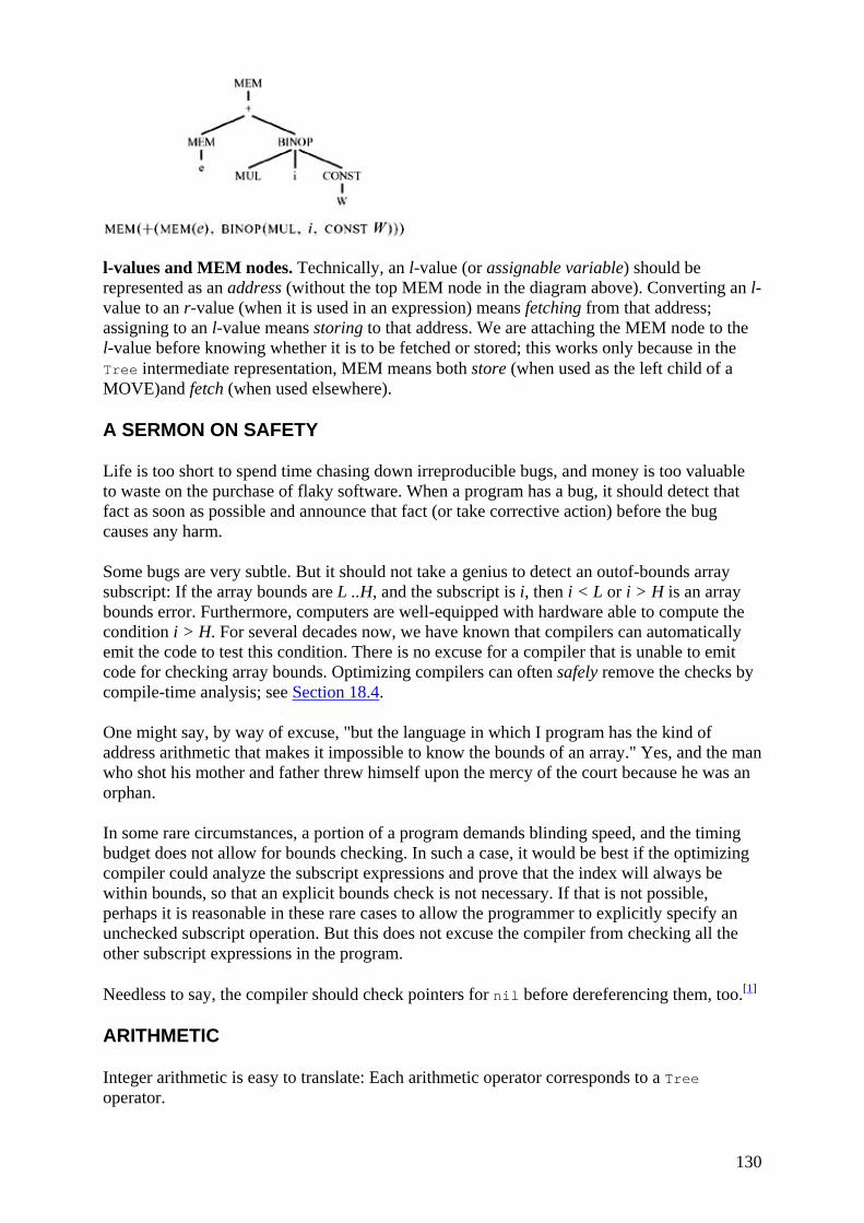
130

l-values and MEM nodes. Technically, an l-value (or assignable variable) should be represented as an address (without the top MEM node in the diagram above). Converting an l-value to an r-value (when it is used in an expression) means fetching from that address; assigning to an l-value means storing to that address. We are attaching the MEM node to the l-value before knowing whether it is to be fetched or stored; this works only because in the Tree intermediate representation, MEM means both store (when used as the left child of a MOVE)and fetch (when used elsewhere).

A SERMON ON SAFETY

Life is too short to spend time chasing down irreproducible bugs, and money is too valuable to waste on the purchase of flaky software. When a program has a bug, it should detect that fact as soon as possible and announce that fact (or take corrective action) before the bug causes any harm.

Some bugs are very subtle. But it should not take a genius to detect an outof-bounds array subscript: If the array bounds are L ..H, and the subscript is i, then i < L or i > H is an array bounds error. Furthermore, computers are well-equipped with hardware able to compute the condition i > H. For several decades now, we have known that compilers can automatically emit the code to test this condition. There is no excuse for a compiler that is unable to emit code for checking array bounds. Optimizing compilers can often safely remove the checks by compile-time analysis; see Section 18.4.

One might say, by way of excuse, "but the language in which I program has the kind of address arithmetic that makes it impossible to know the bounds of an array." Yes, and the man who shot his mother and father threw himself upon the mercy of the court because he was an orphan.

In some rare circumstances, a portion of a program demands blinding speed, and the timing budget does not allow for bounds checking. In such a case, it would be best if the optimizing compiler could analyze the subscript expressions and prove that the index will always be within bounds, so that an explicit bounds check is not necessary. If that is not possible, perhaps it is reasonable in these rare cases to allow the programmer to explicitly specify an unchecked subscript operation. But this does not excuse the compiler from checking all the other subscript expressions in the program.

Needless to say, the compiler should check pointers for nil before dereferencing them, too.[1]

ARITHMETIC

Integer arithmetic is easy to translate: Each arithmetic operator corresponds to a Tree operator.

131

The Tree language has no unary arithmetic operators. Unary negation of integers can be implemented as subtraction from zero; unary complement can be implemented as XOR with all ones.

Unary floating-point negation cannot be implemented as subtraction from zero, because many floating-point representations allow a negative zero. The negation of negative zero is positive zero, and vice versa. Thus, the Tree language does not support unary negation very well.

Fortunately, the MiniJava language doesn't support floating-point numbers; but in a real compiler, a new operator would have to be added for floating negation.

CONDITIONALS

The result of a comparison operator will be a Cx expression: a statement s that will jump to any true-destination and false-destination you specify.

Making "simple" Cx expressions from comparison operators is easy with the CJUMP operator. However, the whole point of the Cx representation is that conditional expressions can be combined easily with the MiniJava operator

&&. Therefore, an expression such as x<5 will be translated as Cx(s1), where

for any labels t and f.

To do this, we extend the Cx class to make a subclass RelCx that has private fields to hold the left and right expressions (in this case x and 5) and the comparison operator (in this case Tree.CJUMP.LT). Then we override the unCx method to generate the CJUMP from these data. It is not necessary to make unEx and unNx methods, since these will be inherited from the parent Cx class.

The most straightforward thing to do with an if-expression

if e1 then e2 else e3

is to treat e1 as a Cx expression, and e2 and e3 as Ex expressions. That is, use the unCx method of e1 and the unEx of e2 and e3. Make two labels t and f to which the conditional will branch. Allocate a temporary r, and after label t, move e2 to r; after label f, move e3 to r. Both branches should finish by jumping to a newly created "join" label.

This will produce perfectly correct results. However, the translated code may not be very efficient at all. If e2 and e3 are both "statements" (expressions that return no value), then their representation is likely to be Nx, not Ex. Applying unEx to them will work - a coercion will automatically be applied - but it might be better to recognize this case specially.

Even worse, if e2 or e3 is a Cx expression, then applying the unEx coercion to it will yield a horrible tangle of jumps and labels. It is much better to recognize this case specially.

For example, consider

if x < 5 then a > b else 0

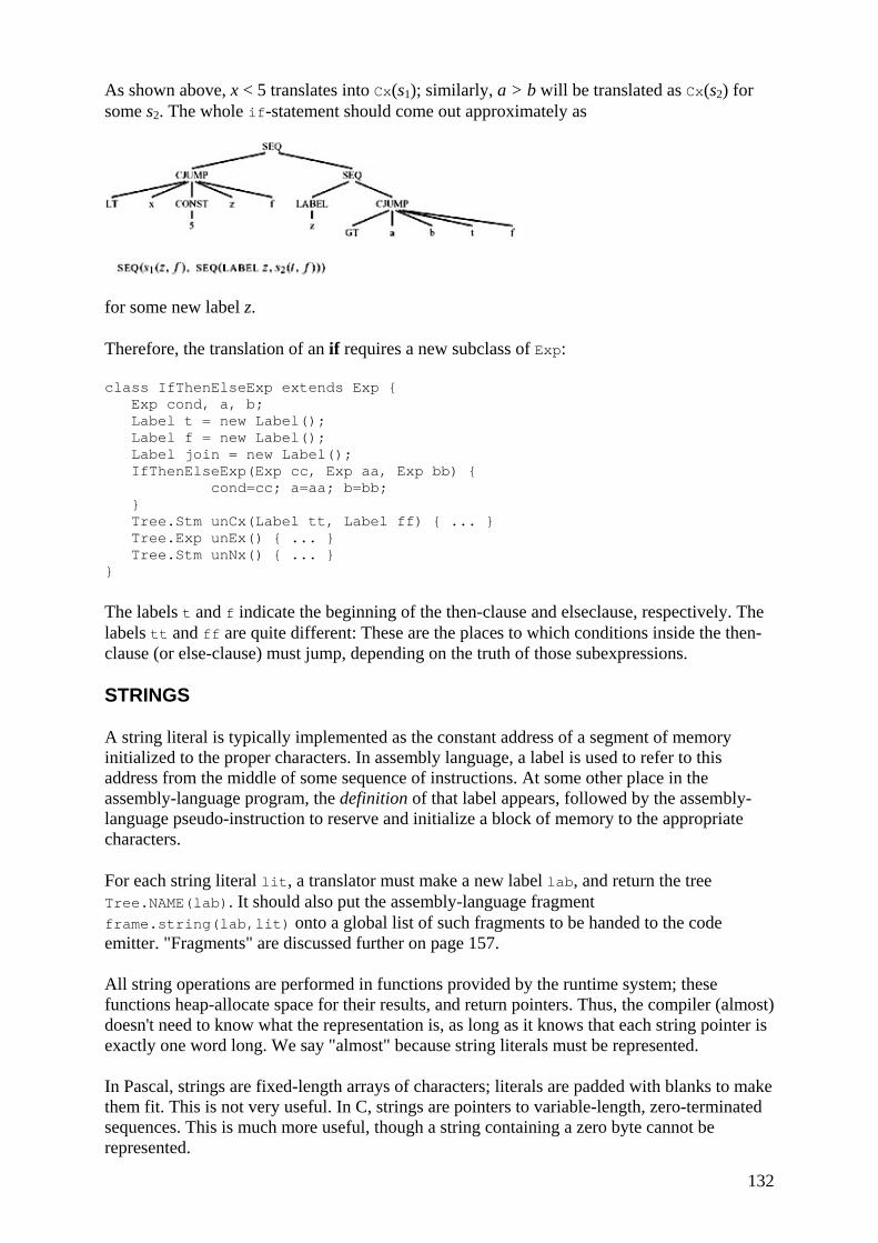
132

As shown above, x < 5 translates into Cx(s1); similarly, a > b will be translated as Cx(s2) for some s2. The whole if-statement should come out approximately as

for some new label z.

Therefore, the translation of an if requires a new subclass of Exp:

class IfThenElseExp extends Exp { Exp cond, a, b; Label t = new Label(); Label f = new Label(); Label join = new Label(); IfThenElseExp(Exp cc, Exp aa, Exp bb) { cond=cc; a=aa; b=bb; } Tree.Stm unCx(Label tt, Label ff) { ... } Tree.Exp unEx() { ... } Tree.Stm unNx() { ... } }

The labels t and f indicate the beginning of the then-clause and elseclause, respectively. The labels tt and ff are quite different: These are the places to which conditions inside the then-clause (or else-clause) must jump, depending on the truth of those subexpressions.

STRINGS

A string literal is typically implemented as the constant address of a segment of memory initialized to the proper characters. In assembly language, a label is used to refer to this address from the middle of some sequence of instructions. At some other place in the assembly-language program, the definition of that label appears, followed by the assembly-language pseudo-instruction to reserve and initialize a block of memory to the appropriate characters.

For each string literal lit, a translator must make a new label lab, and return the tree Tree.NAME(lab). It should also put the assembly-language fragment frame.string(lab,lit) onto a global list of such fragments to be handed to the code emitter. "Fragments" are discussed further on page 157.

All string operations are performed in functions provided by the runtime system; these functions heap-allocate space for their results, and return pointers. Thus, the compiler (almost) doesn't need to know what the representation is, as long as it knows that each string pointer is exactly one word long. We say "almost" because string literals must be represented.

In Pascal, strings are fixed-length arrays of characters; literals are padded with blanks to make them fit. This is not very useful. In C, strings are pointers to variable-length, zero-terminated sequences. This is much more useful, though a string containing a zero byte cannot be represented.

133

RECORD AND ARRAY CREATION

Imagine a language construct {e1, e2, …, en} which creates an n-element record initialized to the values of expressions ei. This is like an object constructor that initializes all the instance variables of the object. Such a record may outlive the procedure activation that creates it, so it cannot be allocated on the stack. Instead, it must be allocated on the heap. If there is no provision for freeing records (or strings), industrial-strength systems should have a garbage collector to reclaim unreachable records (see Chapter 13).

The simplest way to create a record is to call an external memory-allocation function that returns a pointer to an n-word area into a new temporary r. Then a series of MOVE trees can initialize offsets 0, 1W; 2W, …, (n − 1)W from r with the translations of expressions ei. Finally, the result of the whole expression is TEMP(r), as shown in Figure 7.4.

Figure 7.4: Object initialization.

In an industrial compiler, calling malloc (or its equivalent) on every record creation might be too slow; see Section 13.7.

Array creation is very much like record creation, except that all the fields are initialized to the same value. The external initArray function can take the array length and the initializing value as arguments, see later.

In MiniJava we can create an array of integers by the construct

new int [exp]

where exp is an expression that evaluates to an integer. This will create an integer array of a length determined by the value of exp and with each value initialized to zero.

To translate array creation, the compiler needs to perform the following steps:

1. Determine how much space is needed for the array. This can be calculated by:

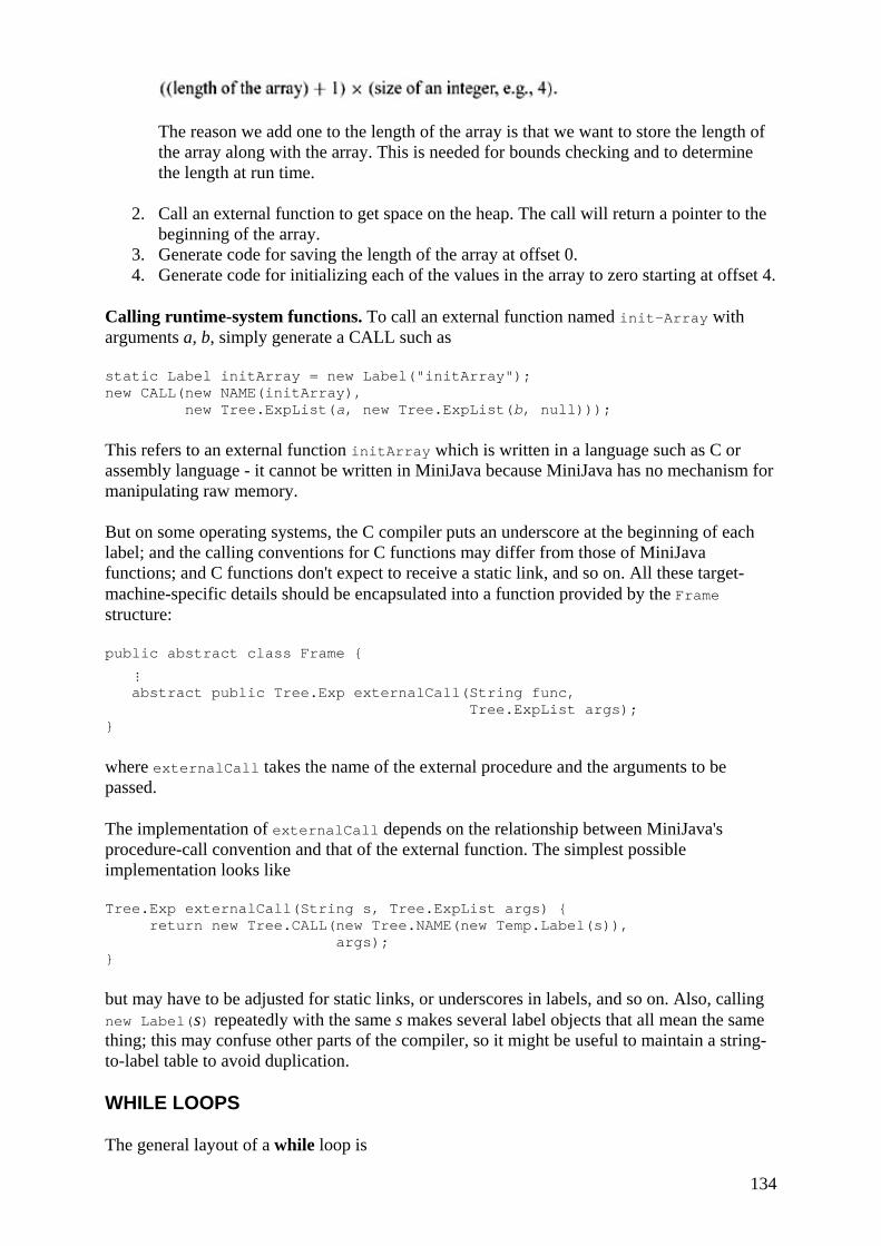
134

The reason we add one to the length of the array is that we want to store the length of the array along with the array. This is needed for bounds checking and to determine the length at run time.

2. Call an external function to get space on the heap. The call will return a pointer to the beginning of the array.

3. Generate code for saving the length of the array at offset 0. 4. Generate code for initializing each of the values in the array to zero starting at offset 4.

Calling runtime-system functions. To call an external function named init-Array with arguments a, b, simply generate a CALL such as

static Label initArray = new Label("initArray"); new CALL(new NAME(initArray), new Tree.ExpList(a, new Tree.ExpList(b, null)));

This refers to an external function initArray which is written in a language such as C or assembly language - it cannot be written in MiniJava because MiniJava has no mechanism for manipulating raw memory.

But on some operating systems, the C compiler puts an underscore at the beginning of each label; and the calling conventions for C functions may differ from those of MiniJava functions; and C functions don't expect to receive a static link, and so on. All these target-machine-specific details should be encapsulated into a function provided by the Frame structure:

public abstract class Frame {

⋮ abstract public Tree.Exp externalCall(String func, Tree.ExpList args); }

where externalCall takes the name of the external procedure and the arguments to be passed.

The implementation of externalCall depends on the relationship between MiniJava's procedure-call convention and that of the external function. The simplest possible implementation looks like

Tree.Exp externalCall(String s, Tree.ExpList args) { return new Tree.CALL(new Tree.NAME(new Temp.Label(s)), args); }

but may have to be adjusted for static links, or underscores in labels, and so on. Also, calling new Label(s) repeatedly with the same s makes several label objects that all mean the same thing; this may confuse other parts of the compiler, so it might be useful to maintain a string-to-label table to avoid duplication.

WHILE LOOPS

The general layout of a while loop is

135

test: if not(condition) goto done body goto test done:

If a break statement occurs within the body (and not nested within any interior while statements), the translation is simply a JUMP to done.

Translation of break statements needs to have a new formal parameter break that is the done label of the nearest enclosing loop. In translating a while loop, the translator will be called recursively upon body with the done label passed as the break parameter. When the translator is recursively calling itself in nonloop contexts, it can simply pass down the same break parameter that was passed to it.

FOR LOOPS

A for statement can be expressed using other kinds of statements:

A straightforward approach to the translation of for statements is to rewrite the abstract syntax into the abstract syntax of the while statement shown, and then translate the result.

This is almost right, but consider the case where limit=maxint. Then i + 1 will overflow; either a hardware exception will be raised, or i ≤ limit will always be true! The solution is to put the test at the bottom of the loop, where i < limit can be tested before the increment. Then an extra test will be needed before entering the loop to check lo ≤ hi.

FUNCTION CALL

Translating a function call f(a1, …an) is simple:

where lf is the label for f. In an object-oriented language, the implicit variable this must be made an explicit argument of the call. That is, p.m(a1, …an) is translated as

where p belongs to class c, and c$m is the m method of class c. For a static method, the computation of address lc$m can be done at compile time - it's a simple label, as it is in MiniJava. For dynamic methods, the computation is more complicated, as explained in Chapter 14.

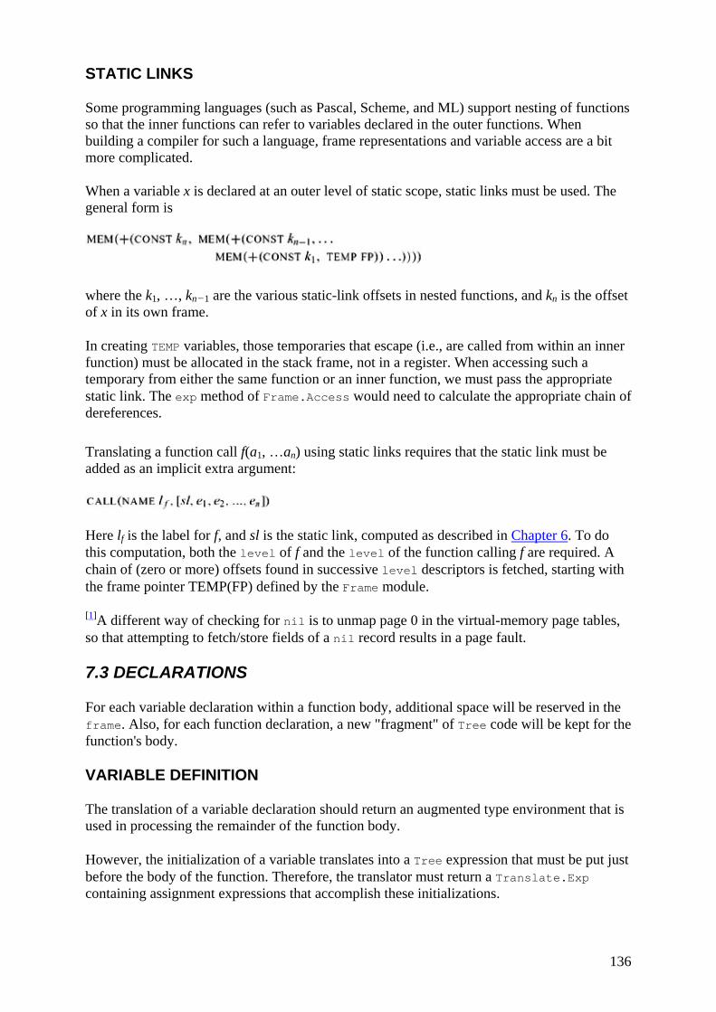
136

STATIC LINKS

Some programming languages (such as Pascal, Scheme, and ML) support nesting of functions so that the inner functions can refer to variables declared in the outer functions. When building a compiler for such a language, frame representations and variable access are a bit more complicated.

When a variable x is declared at an outer level of static scope, static links must be used. The general form is

where the k1, …, kn−1 are the various static-link offsets in nested functions, and kn is the offset of x in its own frame.

In creating TEMP variables, those temporaries that escape (i.e., are called from within an inner function) must be allocated in the stack frame, not in a register. When accessing such a temporary from either the same function or an inner function, we must pass the appropriate static link. The exp method of Frame.Access would need to calculate the appropriate chain of dereferences.

Translating a function call f(a1, …an) using static links requires that the static link must be added as an implicit extra argument:

Here lf is the label for f, and sl is the static link, computed as described in Chapter 6. To do this computation, both the level of f and the level of the function calling f are required. A chain of (zero or more) offsets found in successive level descriptors is fetched, starting with the frame pointer TEMP(FP) defined by the Frame module.

[1]A different way of checking for nil is to unmap page 0 in the virtual-memory page tables, so that attempting to fetch/store fields of a nil record results in a page fault.

7.3 DECLARATIONS

For each variable declaration within a function body, additional space will be reserved in the frame. Also, for each function declaration, a new "fragment" of Tree code will be kept for the function's body.

VARIABLE DEFINITION

The translation of a variable declaration should return an augmented type environment that is used in processing the remainder of the function body.

However, the initialization of a variable translates into a Tree expression that must be put just before the body of the function. Therefore, the translator must return a Translate.Exp containing assignment expressions that accomplish these initializations.

137

If the translator is applied to function and type declarations, the result will be a "no-op" expression such as Ex(CONST(0)).

FUNCTION DEFINITION

A function is translated into a segment of assembly language with a prologue, a body, andan epilogue. The body of a function is an expression, and the body of the translation is simply the translation of that expression.

The prologue, which precedes the body in the assembly-language version of the function, contains

1. pseudo-instructions, as needed in the particular assembly language, to announce the beginning of a function;

2. a label definition for the function name; 3. an instruction to adjust the stack pointer (to allocate a new frame); 4. instructions to save "escaping" arguments into the frame, and to move nonescaping

arguments into fresh temporary registers; 5. store instructions to save any callee-save registers - including the return address

register - used within the function. Then comes

6. the function body. The epilogue comes after the body and contains

7. an instruction to move the return value (result of the function) to the register reserved for that purpose;

8. load instructions to restore the callee-save registers; 9. an instruction to reset the stack pointer (to deallocate the frame); 10. a return instruction (JUMP to the return address); 11. pseudo-instructions, as needed, to announce the end of a function.

Some of these items (1, 3, 9, and 11) depend on exact knowledge of the frame size, which will not be known until after the register allocator determines how many local variables need to be kept in the frame because they don't fit in registers. So these instructions should be generated very late, in a FRAME function called procEntryExit3 (see also page 252). Item 2 (and 10), nestled between 1 and 3 (and 9 and 11, respectively) are also handled at that time.

To implement 7, the Translate phase should generate a move instruction

MOVE(RV, body)

that puts the result of evaluating the body in the return value (RV) location specified by the machine-specific frame structure:

package Frame; public abstract class Frame {

⋮ abstract public Temp RV(); }

Item 4 (moving incoming formal parameters), and 5 and 8 (the saving and restoring of callee-save registers), are part of the view shift described on page 128. They should be done by a function in the Frame module:

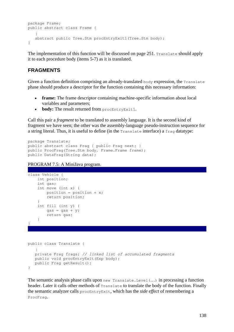
138

package Frame; public abstract class Frame {

⋮ abstract public Tree.Stm procEntryExit1(Tree.Stm body); }

The implementation of this function will be discussed on page 251. Translate should apply it to each procedure body (items 5-7) as it is translated.

FRAGMENTS

Given a function definition comprising an already-translated body expression, the Translate phase should produce a descriptor for the function containing this necessary information:

• frame: The frame descriptor containing machine-specific information about local variables and parameters;

• body: The result returned from procEntryExit1.

Call this pair a fragment to be translated to assembly language. It is the second kind of fragment we have seen; the other was the assembly-language pseudo-instruction sequence for a string literal. Thus, it is useful to define (in the Translate interface) a frag datatype:

package Translate; public abstract class Frag { public Frag next; } public ProcFrag(Tree.Stm body, Frame.Frame frame); public DataFrag(String data); PROGRAM 7.5: A MiniJava program. class Vehicle { int position; int gas; int move (int x) { position = position + x; return position; } int fill (int y) { gas = gas + y; return gas; } }

public class Translate {

⋮ private Frag frags; // linked list of accumulated fragments public void procEntryExit(Exp body); public Frag getResult(); }

The semantic analysis phase calls upon new Translate.Level(…) in processing a function header. Later it calls other methods of Translate to translate the body of the function. Finally the semantic analyzer calls procEntryExit, which has the side effect of remembering a ProcFrag.

139

All the remembered fragments go into a private fragment list within Translate;then getResult can be used to extract the fragment list.

CLASSES AND OBJECTS

Figure 7.5 shows a MiniJava class Vehicle with two instance variables position and gas, and two methods move and fill. We can create multiple Vehicle objects. Each Vehicle object will have its own position and gas variables. Two Vehicle objects can have different values in their variables, and in MiniJava, only the methods of an object can access the variables of that object. The translation of new Vehicle() is much like the translation of record creation and can be done in two steps:

1. Generate code for allocating heap space for all the instance variables; in this case we need to allocate 8 bytes (2 integers, each of size, say, 4).

2. Iterate through the memory locations for those variables and initialize them- in this case, they should both be initialized to 0.

Methods and the this pointer. Method calls in MiniJava are similar to function calls; but first, we must determine the class in which the method is declared and look up the method in that class. Second, we need to address the following question. Suppose we have multiple Vehicle objects and we want to call a method on one of them; how do we ensure that the implementation knows for which object we are calling the method? The solution is to pass that object as an extra argument to the method; that argument is the this pointer. For a method call

Vehicle v; ... v.move();

the Vehicle object in variable v will be the this pointer when calling the move method.

The translation of method declarations is much like the translation of functions, but we need to avoid name clashes among methods with the same name that are declared in different classes. We can do that by choosing a naming scheme such that the name of the translated method is the concatenation of the class name and the method name. For example, the translation of move can be given the name Vehicle move.

Accessing variables In MiniJava, variables can be accessed from methods in the same class. Variables are accessed via the this pointer; thus, the translation of a variable reference is like field selection for records. The position of the variable in the object can be looked up in the symbol table for the class.

PROGRAM TRANSLATION TO TREES

Design a set of visitors which translate a MiniJava program into intermediate representation trees.

Supporting files in $MINIJAVA/chap7 include:

Tree/* Data types for the Tree language. Tree/Print.java Functions to display trees for debugging.

140

A simpler translator To simplify the implementation of the translator, you may do without the Ex, Nx, Cx constructors. The entire translation can be done with ordinary value expressions. This means that there is only one Exp class (without subclasses); this class contains one field of type Tree.Exp and only an unEx() method. Instead of Nx(s), use Ex(ESEQ(s, CONST 0)). For conditionals, instead of a Cx, use an expression that just evaluates to 1 or 0.

The intermediate representation trees produced from this kind of naive translation will be bulkier and slower than a "fancy" translation. But they will work correctly, and in principle a fancy back-end optimizer might be able to clean up the clumsiness. In any case, a clumsy but correct translator is better than a fancy one that doesn't work.

EXERCISES

• 7.1 Suppose a certain compiler translates all statements and expressions into Tree.Exp trees, and does not use the Nx and Cx constructors to represent expressions in different ways. Draw a picture of the IR tree that results from each of the following MiniJava statements and expressions.

a. a+5 b. b[i+1] c. a<b, which should be implemented by making an ESEQ whose left-hand side

moves a 1 or 0 into some newly defined temporary, and whose right-hand side is the temporary.

d. a = x+y; which should be translated with an EXP node at the top. e. if (a<b) c=a; else c=b; translated using the a<b tree from part (c) above;

the whole statement will therefore be rather clumsy and inefficient. f. if (a<b) c=a; else c=b; translated in a less clumsy way.

• 7.2 Translate each of these MiniJava statements and expressions into IR trees, but using the Ex, Nx, and Cx constructors as appropriate. In each case, just draw pictures of the trees; an Ex tree will be a Tree Exp, an Nx tree will be a Tree Stm, anda Cx tree will be a Stm with holes labeled trueand falseinto which labels can later be placed.

a. a+5; b. b[i+1]=0; c. while (a<0) a=a+1; d. a<b moves a 1 or 0 into some newly defined temporary, and whose right-hand

side is the temporary. e. a = x+y; f. if (a<b) c=a; else c=b;

• 7.3 Using the C compiler of your choice (or a compiler for another language), translate some functions to assembly language. On Unix this is done with the -S option to the C compiler.

Then identify all the components of the calling sequence (items 1-11), and explain what each line of assembly language does (especially the pseudoinstructions that comprise items 1 and 11). Try one small function that returns without much computation (a leaffunction), and one that calls another function before eventually returning.

• 7.4 The Tree intermediate language has no operators for floating-point variables. Show how the language would look with new binops for floating-point arithmetic, and new relops for floating-point comparisons. You may find it useful to introduce a variant of MEM nodes to describe fetching and storing floating-point values.

141

• *7.5 The Tree intermediate language has no provision for data values that are not exactly one word long. The C programming language has signed and unsigned integers of several sizes, with conversion operators among the different sizes. Augment the intermediate language to accommodate several sizes of integers, with conversions among them.

Hint: Do not distinguish signed values from unsigned values in the intermediate trees, but do distinguish between signed operators and unsigned operators. See also Fraser and Hanson [1995], Sections 5.5 and 9.1.

142

Chapter 8: Basic Blocks and Traces ca-non-i-cal: reduced to the simplest or clearest schema possible


OVERVIEW

The trees generated by the semantic analysis phase must be translated into assembly or machine language. The operators of the Tree language are chosen carefully to match the capabilities of most machines. However, there are certain aspects of the tree language that do not correspond exactly with machine languages, and some aspects of the Tree language interfere with compiletime optimization analyses.

For example, it's useful to be able to evaluate the subexpressions of an expression in any order. But the subexpressions of Tree.exp can contain side effects - ESEQ and CALL nodes that contain assignment statements and perform input/output. If tree expressions did not contain ESEQ and CALL nodes, then the order of evaluation would not matter.

Some of the mismatches between Trees and machine-language programs are

• The CJUMP instruction can jump to either of two labels, but real machines' conditional jump instructions fall through to the next instruction if the condition is false.

• ESEQ nodes within expressions are inconvenient, because they make different orders of evaluating subtrees yield different results.

• CALL nodes within expressions cause the same problem. • CALL nodes within the argument-expressions of other CALL nodes will cause

problems when trying to put arguments into a fixed set of formal-parameter registers.

Why does the Tree language allow ESEQ and two-way CJUMP, if they are so troublesome? Because they make it much more convenient for the Translate (translation to intermediate code) phase of the compiler.

We can take any tree and rewrite it into an equivalent tree without any of the cases listed above. Without these cases, the only possible parent of a SEQ node is another SEQ; all the SEQ nodes will be clustered at the top of the tree. This makes the SEQs entirely uninteresting; we might as well get rid of them and make a linear list of Tree.Stms.

The transformation is done in three stages: First, a tree is rewritten into a list of canonical trees without SEQ or ESEQ nodes; then this list is grouped into a set of basic blocks, which contain no internal jumps or labels; then the basic blocks are ordered into a set of traces in which every CJUMP is immediately followed by its false label.

Thus the module Canon has these tree-rearrangement functions:

package Canon; public class Canon { static public Tree.StmList linearize(Tree.Stm s); } public class BasicBlocks { public StmListList blocks;

143

public Temp.Label done; public BasicBlocks(Tree.StmList stms); } StmListList(Tree.StmList head, StmListList tail); public class TraceSchedule { public TraceSchedule(BasicBlocks b); public Tree.StmList stms; }

Linearize removes the ESEQs and moves the CALLs to top level. Then BasicBlocks groups statements into sequences of straight-line code. Finally, TraceSchedule orders the blocks so that every CJUMP is followed by its false label.

8.1 CANONICAL TREES

Let us define canonical trees as having these properties:

1. No SEQ or ESEQ. 2. The parent of each CALL is either EXP(…) or MOVE(TEMP t,…).

TRANSFORMATIONS ON ESEQ

How can the ESEQ nodes be eliminated? The idea is to lift them higher and higher in the tree, until they can become SEQ nodes.

Figure 8.1 gives some useful identities on trees.

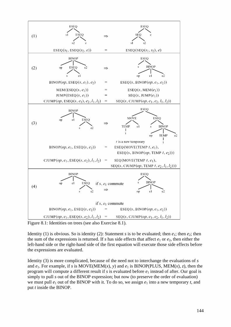
144

Figure 8.1: Identities on trees (see also Exercise 8.1).

Identity (1) is obvious. So is identity (2): Statement s is to be evaluated; then e1; then e2; then the sum of the expressions is returned. If s has side effects that affect e1 or e2, then either the left-hand side or the right-hand side of the first equation will execute those side effects before the expressions are evaluated.

Identity (3) is more complicated, because of the need not to interchange the evaluations of s and e1. For example, if s is MOVE(MEM(x), y) and e1 is BINOP(PLUS, MEM(x), z), then the program will compute a different result if s is evaluated before e1 instead of after. Our goal is simply to pull s out of the BINOP expression; but now (to preserve the order of evaluation) we must pull e1 out of the BINOP with it. To do so, we assign e1 into a new temporary t, and put t inside the BINOP.

145

It may happen that s causes no side effects that can alter the result produced by e1. This will happen if the temporaries and memory locations assigned by s are not referenced by e1 (and s and e1 don't both perform external I/O). In this case, identity (4) can be used.

We cannot always tell if two expressions commute. For example, whether MOVE(MEM(x), y) commutes with MEM(z) depends on whether x = z, which we cannot always determine at compile time. So we conservatively approximate whether statements commute, saying either "they definitely do commute" or "perhaps they don't commute." For example, we know that any statement "definitely commutes" with the expression CONST(n), so we can use identity (4) to justify special cases like

The commute function estimates (very naively) whether a statement commutes with an expression:

static boolean commute(Tree.Stm a, Tree.Exp b) { return isNop(a) || b instanceof Tree.NAME || b instanceof Tree.CONST; } static boolean isNop(Tree.Stm a) { return a instanceof Tree.EXP && ((Tree.EXP)a).exp instanceof Tree.CONST; }

A constant commutes with any statement, and the empty statement commutes with any expression. Anything else is assumed not to commute.

GENERAL REWRITING RULES

In general, for each kind of Tree statement or expression we can identify the subexpressions. Then we can make rewriting rules, similar to the ones in Figure 8.1, to pull the ESEQs out of the statement or expression.

For example, in [e1, e2, ESEQ(s, e3)], the statement s must be pulled leftward past e2 and e1. If they commute, we have (s; [e1, e2, e3]). But suppose e2 does not commute with s; then we must have

Or if e2 commutes with s but e1 does not, we have

The reorder function takes a list of expressions and returns a pair of (statement, expression-list). The statement contains all the things that must be executed before the expression-list. As shown in these examples, this includes all the statement-parts of the ESEQs, as well as any expressions to their left with which they did not commute. When there are no ESEQs at all we will use EXP(CONST 0), which does nothing, as the statement.

Algorithm Step one is to make a "subexpression-extraction" method for each kind. Step two is to make a "subexpression-insertion" method: Given an ESEQ-clean version of each subexpression, this builds a new version of the expression or statement.

146

These will be methods of the Tree.Exp and Tree.Stm classes:

package Tree; abstract public class Exp { abstract public ExpList kids(); abstract public Exp build(ExpList kids); } abstract public class Stm { abstract public ExpList kids(); abstract public Stm build(ExpList kids); }

Each subclass Exp or Stm must implement the methods; for example,

package Tree; public class BINOP extends Exp { public int binop; public Exp left, right; public BINOP(int b, Exp l, Exp r) {binop=b; ...} public final static int PLUS=0, MINUS=1, MUL=2, DIV=3, AND=4,OR=5,LSHIFT=6,RSHIFT=7,ARSHIFT=8,XOR=9; public ExpList kids() {return new ExpList(left, new ExpList(right,null));} public Exp build(ExpList kids) { return new BINOP(binop,kids.head,kids.tail.head); } }

Other subclasses have similar (or even simpler) kids and build methods. Using these build methods, we can write functions

static Tree.Stm do_stm(Tree.Stm s) static Tree.ESEQ do_exp (Tree.Exp e)

that pull all the ESEQs out of a statement or expression, respectively. That is, do_stm uses s.kids() to get the immediate subexpressions of s, which will be an expression-list l. It then pulls all the ESEQs out of l recursively, yielding a clump of side-effecting statements s1 and a cleaned-up list l′. Then SEQ(s1, s.build(l′)) constructs a new statement, like the original s but with no ESEQs. These functions rely on auxiliary functions reorder_stm and reorder_exp for help; see also Exercise 8.3.

The left-hand operand of the MOVE statement is not considered a subexpression, because it is the destination of the statement - its value is not used by the statement. However, if the destination is a memory location, then the address acts like a source. Thus we have,

public class MOVE extends Stm { public Exp dst, src; public MOVE(Exp d, Exp s) {dst=d; src=s;} public ExpList kids() { if (dst instanceof MEM) return new ExpList(((MEM)dst).exp, new ExpList(src,null)); else return new ExpList(src,null); } public Stm build(ExpList kids) { if (dst instanceof MEM) return new MOVE(new MEM(kids.head), kids.tail.head); else return new MOVE(dst, kids.head);

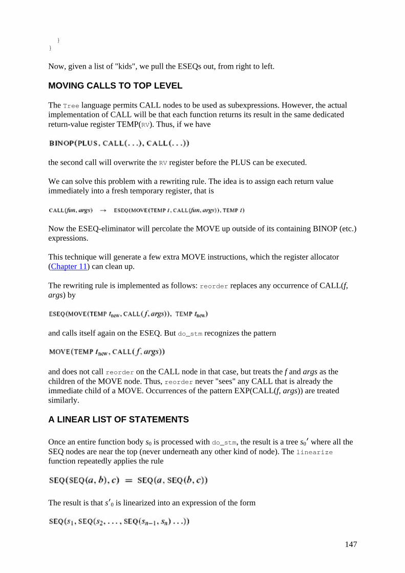
147

} }

Now, given a list of "kids", we pull the ESEQs out, from right to left.

MOVING CALLS TO TOP LEVEL

The Tree language permits CALL nodes to be used as subexpressions. However, the actual implementation of CALL will be that each function returns its result in the same dedicated return-value register TEMP(RV). Thus, if we have

the second call will overwrite the RV register before the PLUS can be executed.

We can solve this problem with a rewriting rule. The idea is to assign each return value immediately into a fresh temporary register, that is

Now the ESEQ-eliminator will percolate the MOVE up outside of its containing BINOP (etc.) expressions.

This technique will generate a few extra MOVE instructions, which the register allocator (Chapter 11) can clean up.

The rewriting rule is implemented as follows: reorder replaces any occurrence of CALL(f, args) by

and calls itself again on the ESEQ. But do_stm recognizes the pattern

and does not call reorder on the CALL node in that case, but treats the f and args as the children of the MOVE node. Thus, reorder never "sees" any CALL that is already the immediate child of a MOVE. Occurrences of the pattern EXP(CALL(f, args)) are treated similarly.

A LINEAR LIST OF STATEMENTS

Once an entire function body s0 is processed with do_stm, the result is a tree s0′ where all the SEQ nodes are near the top (never underneath any other kind of node). The linearize function repeatedly applies the rule

The result is that s′0 is linearized into an expression of the form

148

Here the SEQ nodes provide no structuring information at all, and we can just consider this to be a simple list of statements,

where none of the si contain SEQ or ESEQ nodes.

These rewrite rules are implemented by linearize, with an auxiliary function linear:

static Tree.StmList linear(Tree.SEQ s, Tree.StmList l) { return linear(s.left,linear(s.right,l)); } static Tree.StmList linear(Tree.Stm s, Tree.StmList l) { if (s instanceof Tree.SEQ) return linear((Tree.SEQ)s,l); else return new Tree.StmList(s,l); } static public Tree.StmList linearize(Tree.Stm s) { return linear(do_stm(s), null); }

8.2 TAMING CONDITIONAL BRANCHES

Another aspect of the Tree language that has no direct equivalent in most machine instruction sets is the two-way branch of the CJUMP instruction. The Tree language CJUMP is designed with two target labels for convenience in translating into trees and analyzing trees. On a real machine, the conditional jump either transfers control (on a true condition) or "falls through" to the next instruction.

To make the trees easy to translate into machine instructions, we will rearrange them so that every CJUMP(cond, lt, lf) is immediately followed by LABEL(lf), its "false branch." Each such CJUMP can be directly implemented on a real machine as a conditional branch to label lt.

We will make this transformation in two stages: First, we take the list of canonical trees and form them into basic blocks; then we order the basic blocks into a trace. The next sections will define these terms.

BASIC BLOCKS

In determining where the jumps go in a program, we are analyzing the program's control flow. Control flow is the sequencing of instructions in a program, ignoring the data values in registers and memory, and ignoring the arithmetic calculations. Of course, not knowing the data values means we cannot know whether the conditional jumps will go to their true or false labels; so we simply say that such jumps can go either way.

In analyzing the control flow of a program, any instruction that is not a jump has an entirely uninteresting behavior. We can lump together any sequence of nonbranch instructions into a basic block and analyze the control flow between basic blocks.

A basic block is a sequence of statements that is always entered at the beginning and exited at the end, that is:

• The first statement is a LABEL. • The last statement is a JUMP or CJUMP.

149

• There are no other LABELs, JUMPs, or CJUMPs.

The algorithm for dividing a long sequence of statements into basic blocks is quite simple. The sequence is scanned from beginning to end; whenever a LABEL is found, a new block is started (and the previous block is ended); whenever a JUMP or CJUMP is found, a block is ended (and the next block is started). If this leaves any block not ending with a JUMP or CJUMP, then a JUMP to the next block's label is appended to the block. If any block has been left without a LABEL at the beginning, a new label is invented and stuck there.

We will apply this algorithm to each function-body in turn. The procedure "epilogue" (which pops the stack and returns to the caller) will not be part of this body, but is intended to follow the last statement. When the flow of program execution reaches the end of the last block, the epilogue should follow. But it is inconvenient to have a "special" block that must come last and that has no JUMP at the end. Thus, we will invent a new label done - intended to mean the beginning of the epilogue - and put a JUMP(NAME done) at the end of the last block.

In the MiniJava compiler, the class Canon.BasicBlocks implements this simple algorithm.

TRACES

Now the basic blocks can be arranged in any order, and the result of executing the program will be the same - every block ends with a jump to the appropriate place. We can take advantage of this to choose an ordering of the blocks satisfying the condition that each CJUMP is followed by its false label.

At the same time, we can also arrange that many of the unconditional JUMPs are immediately followed by their target label. This will allow the deletion of these jumps, which will make the compiled program run a bit faster.

A trace is a sequence of statements that could be consecutively executed during the execution of the program. It can include conditional branches. A program has many different, overlapping traces. For our purposes in arranging CJUMPs and false-labels, we want to make a set of traces that exactly covers the program: Each block must be in exactly one trace. To minimize the number of JUMPs from one trace to another, we would like to have as few traces as possible in our covering set.

A very simple algorithm will suffice to find a covering set of traces. The idea is to start with some block - the beginning of a trace - and follow a possible execution path - the rest of the trace. Suppose block b1 ends with a JUMP to b4, and b4 has a JUMP to b6. Then we can make the trace b1, b4, b6.

But suppose b6 ends with a conditional jump CJUMP(cond, b7, b3). We cannot know at compile time whether b7 or b3 will be next. But we can assume that some execution will follow b3, so let us imagine it is that execution that we are simulating. Thus, we append b3 to our trace and continue with the rest of the trace after b3. The block b7 will be in some other trace.

Algorithm 8.2 (which is similar to Canon.TraceSchedule) ordersthe blocks into traces as follows: It starts with some block and follows a chain of jumps, marking each block and appending it to the current trace. Eventually it comes to a block whose successors are all marked, so it ends the trace and picks an unmarked block to start the next trace.

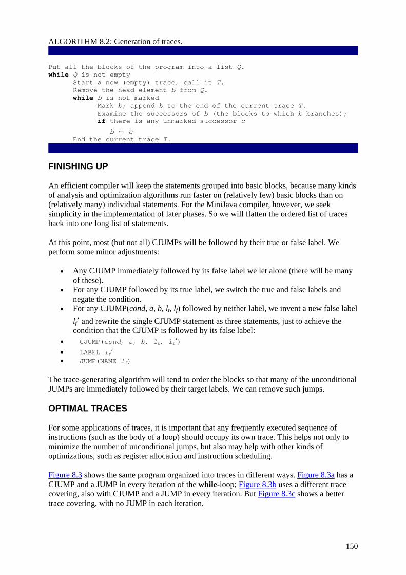
150

ALGORITHM 8.2: Generation of traces. Put all the blocks of the program into a list Q. while Q is not empty Start a new (empty) trace, call it T. Remove the head element b from Q. while b is not marked Mark b; append b to the end of the current trace T. Examine the successors of b (the blocks to which b branches); if there is any unmarked successor c

b ← c End the current trace T.

FINISHING UP

An efficient compiler will keep the statements grouped into basic blocks, because many kinds of analysis and optimization algorithms run faster on (relatively few) basic blocks than on (relatively many) individual statements. For the MiniJava compiler, however, we seek simplicity in the implementation of later phases. So we will flatten the ordered list of traces back into one long list of statements.

At this point, most (but not all) CJUMPs will be followed by their true or false label. We perform some minor adjustments:

• Any CJUMP immediately followed by its false label we let alone (there will be many of these).

• For any CJUMP followed by its true label, we switch the true and false labels and negate the condition.

• For any CJUMP(cond, a, b, lt, lf) followed by neither label, we invent a new false label lf′ and rewrite the single CJUMP statement as three statements, just to achieve the condition that the CJUMP is followed by its false label:

• CJUMP(cond, a, b, lt, lf′) • LABEL lf′ • JUMP(NAME lf)

The trace-generating algorithm will tend to order the blocks so that many of the unconditional JUMPs are immediately followed by their target labels. We can remove such jumps.

OPTIMAL TRACES

For some applications of traces, it is important that any frequently executed sequence of instructions (such as the body of a loop) should occupy its own trace. This helps not only to minimize the number of unconditional jumps, but also may help with other kinds of optimizations, such as register allocation and instruction scheduling.

Figure 8.3 shows the same program organized into traces in different ways. Figure 8.3a has a CJUMP and a JUMP in every iteration of the while-loop; Figure 8.3b uses a different trace covering, also with CJUMP and a JUMP in every iteration. But Figure 8.3c shows a better trace covering, with no JUMP in each iteration.

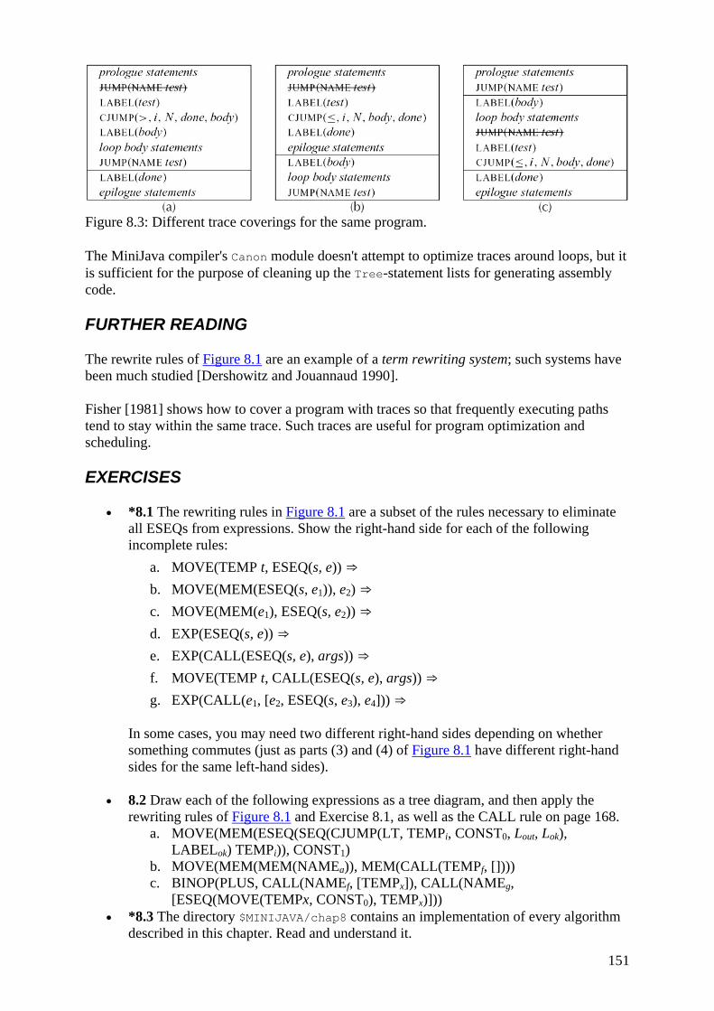
151

Figure 8.3: Different trace coverings for the same program.

The MiniJava compiler's Canon module doesn't attempt to optimize traces around loops, but it is sufficient for the purpose of cleaning up the Tree-statement lists for generating assembly code.

FURTHER READING

The rewrite rules of Figure 8.1 are an example of a term rewriting system; such systems have been much studied [Dershowitz and Jouannaud 1990].

Fisher [1981] shows how to cover a program with traces so that frequently executing paths tend to stay within the same trace. Such traces are useful for program optimization and scheduling.

EXERCISES

• *8.1 The rewriting rules in Figure 8.1 are a subset of the rules necessary to eliminate all ESEQs from expressions. Show the right-hand side for each of the following incomplete rules:

a. MOVE(TEMP t, ESEQ(s, e)) ⇒ b. MOVE(MEM(ESEQ(s, e1)), e2) ⇒ c. MOVE(MEM(e1), ESEQ(s, e2)) ⇒ d. EXP(ESEQ(s, e)) ⇒ e. EXP(CALL(ESEQ(s, e), args)) ⇒ f. MOVE(TEMP t, CALL(ESEQ(s, e), args)) ⇒ g. EXP(CALL(e1, [e2, ESEQ(s, e3), e4])) ⇒

In some cases, you may need two different right-hand sides depending on whether something commutes (just as parts (3) and (4) of Figure 8.1 have different right-hand sides for the same left-hand sides).

• 8.2 Draw each of the following expressions as a tree diagram, and then apply the rewriting rules of Figure 8.1 and Exercise 8.1, as well as the CALL rule on page 168.

a. MOVE(MEM(ESEQ(SEQ(CJUMP(LT, TEMPi, CONST0, Lout, Lok), LABELok) TEMPi)), CONST1)

b. MOVE(MEM(MEM(NAMEa)), MEM(CALL(TEMPf, []))) c. BINOP(PLUS, CALL(NAMEf, [TEMPx]), CALL(NAMEg,

[ESEQ(MOVE(TEMPx, CONST0), TEMPx)])) • *8.3 The directory $MINIJAVA/chap8 contains an implementation of every algorithm

described in this chapter. Read and understand it.

152

• 8.4 A primitive form of the commute test is shown on page 164. This function is conservative: If interchanging the order of evaluation of the expressions will change the result of executing the program, this function will definitely return false; but if an interchange is harmless, commute might return true or false.

Write a more powerful version of commute that returns true in more cases, but is still conservative. Document your program by drawing pictures of (pairs of) expression trees on which it will return true.

• *8.5 The left-hand side of a MOVE node really represents a destination, not an expression. Consequently, the following rewrite rule is nota good idea:

• MOVE(e1, ESEQ(s, e2)) → SEQ(s, MOVE(e1, e2)) if s, e1 commute

Write a statement matching the left side of this rewrite rule that produces a different result when rewritten.

Hint: It is very reasonable to say that the statement MOVE(TEMPa, TEMPb) commutes with expression TEMPb (if a and b are not the same), since TEMPb yields the same value whether executed before or after the MOVE.

Conclusion: The only subexpression of MOVE(TEMPa, e) is e, and the subexpressions of MOVE(MEM(e1), e2) are [e1, e2]; we should not say that a is a subexpression of MOVE(a, b).

• 8.6 Break this program into basic blocks. 1. m ← 0 2. v ← 0 3. if v ≥ n goto 15 4. r ← v 5. s ← 0 6. if r < n goto 9 7. v ← v + 1 8. goto 3 9. x ← M[r] 10. s ← s + x 11. if s ≤ m goto 13 12. m ← s 13. r ← r + 1 14. goto 6 15. return m

• 8.7 Express the basic blocks of Exercise 8.6 as statements in the Tree intermediate form, and use Algorithm 8.2 to generate a set of traces.

153

Chapter 9: Instruction Selection in-struc-tion: a code that tells a computer to perform a particular operation


OVERVIEW

The intermediate representation (Tree) language expresses only one operation in each tree node: memory fetch or store, addition or subtraction, conditional jump, and so on. A real machine instruction can often perform several of these primitive operations. For example, almost any machine can perform an add and a fetch in the same instruction, corresponding to the tree

Finding the appropriate machine instructions to implement a given intermediate representation tree is the job of the instruction selection phase of a compiler.

TREE PATTERNS

We can express a machine instruction as a fragment of an IR tree, called a tree pattern. Then instruction selection becomes the task of tiling the tree with a minimal set of tree patterns.

For purposes of illustration, we invent an instruction set: the Jouette architecture. The arithmetic and memory instructions of Jouette are shown in Figure 9.1. On this machine, register r0 always contains zero.

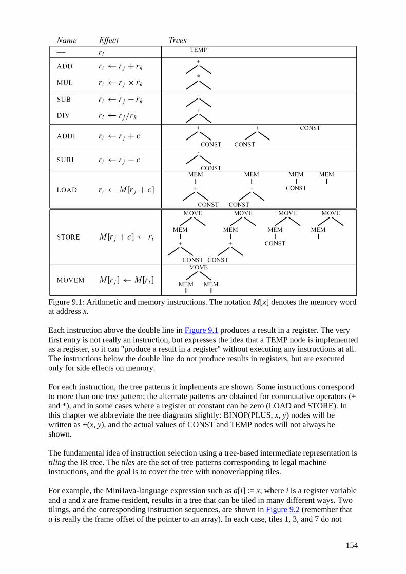
154

Figure 9.1: Arithmetic and memory instructions. The notation M[x] denotes the memory word at address x.

Each instruction above the double line in Figure 9.1 produces a result in a register. The very first entry is not really an instruction, but expresses the idea that a TEMP node is implemented as a register, so it can "produce a result in a register" without executing any instructions at all. The instructions below the double line do not produce results in registers, but are executed only for side effects on memory.

For each instruction, the tree patterns it implements are shown. Some instructions correspond to more than one tree pattern; the alternate patterns are obtained for commutative operators (+ and *), and in some cases where a register or constant can be zero (LOAD and STORE). In this chapter we abbreviate the tree diagrams slightly: BINOP(PLUS, x, y) nodes will be written as +(x, y), and the actual values of CONST and TEMP nodes will not always be shown.

The fundamental idea of instruction selection using a tree-based intermediate representation is tiling the IR tree. The tiles are the set of tree patterns corresponding to legal machine instructions, and the goal is to cover the tree with nonoverlapping tiles.

For example, the MiniJava-language expression such as a[i] := x, where i is a register variable and a and x are frame-resident, results in a tree that can be tiled in many different ways. Two tilings, and the corresponding instruction sequences, are shown in Figure 9.2 (remember that a is really the frame offset of the pointer to an array). In each case, tiles 1, 3, and 7 do not

155

correspond to any machine instructions, because they are just registers (TEMPs) already containing the right values.

Figure 9.2: A tree tiled in two ways.

Finally - assuming a "reasonable" set of tile patterns - it is always possible to tile the tree with tiny tiles, each covering only one node. In our example, such a tiling looks like this:

ADDI r1 ← r0 + a ADD r1 ← fp + r1 LOAD r1 ← M[r1 + 0]ADDI r2 ← r0 + 4 MUL r2 ← ri × r2 ADD r1 ← r1 = r2 ADDI r2 ← r0 + x ADD r2 ← fp + r2 LOAD r2 ← M[r2 + 0]STORE M[r1 + 0] ← r2

For a reasonable set of patterns, it is sufficient that each individual Tree node correspond to some tile. It is usually possible to arrange for this; for example, the LOAD instruction can be made to cover just a single MEM node by using a constant of 0, and so on.

156

OPTIMAL AND OPTIMUM TILINGS

The best tiling of a tree corresponds to an instruction sequence of least cost: the shortest sequence of instructions. Or if the instructions take different amounts of time to execute, the least-cost sequence has the lowest total time.

Suppose we could give each kind of instruction a cost. Then we could define an optimum tiling as the one whose tiles sum to the lowest possible value. An optimal tiling is one where no two adjacent tiles can be combined into a single tile of lower cost. If there is some tree pattern that can be split into several tiles of lower combined cost, then we should remove that pattern from our catalog of tiles before we begin.

Every optimum tiling is also optimal, but not vice versa. For example, suppose every instruction costs one unit, except for MOVEM, which costs m units. Then either Figure 9.2a is optimum (if m > 1) or Figure 9.2b is optimum (if m < 1) or both (if m = 1); but both trees are optimal.

Optimum tiling is based on an idealized cost model. In reality, instructions are not self-contained with individually attributable costs; nearby instructions interact in many ways, as discussed in Chapter 20.

9.1 ALGORITHMS FOR INSTRUCTION SELECTION

There are good algorithms for finding optimum and optimal tilings, but the algorithms for optimal tilings are simpler, as you might expect.

Complex instruction set computers (CISC) have instructions that accomplish several operations each. The tiles for these instructions are quite large, and the difference between optimum and optimal tilings - while never very large - is at least sometimes noticeable.

Most architectures of modern design are reduced instruction set computers (RISC). Each RISC instruction accomplishes just a small number of operations (all the Jouette instructions except MOVEM are typical RISC instructions). Since the tiles are small and of uniform cost, there is usually no difference at all between optimum and optimal tilings. Thus, the simpler tiling algorithms suffice.

MAXIMAL MUNCH

The algorithm for optimal tiling is called maximal munch. It is quite simple. Starting at the root of the tree, find the largest tile that fits. Cover the root node - and perhaps several other nodes near the root - with this tile, leaving several subtrees. Now repeat the same algorithm for each subtree.

As each tile is placed, the instruction corresponding to that tile is generated. The maximal munch algorithm generates the instructions in reverse order - after all, the instruction at the root is the first to be generated, but it can only execute after the other instructions have produced operand values in registers.

The "largest tile" is the one with the most nodes. For example, the tile for ADD has one node, the tile for SUBI has two nodes, and the tiles for STORE and MOVEM have three nodes each.

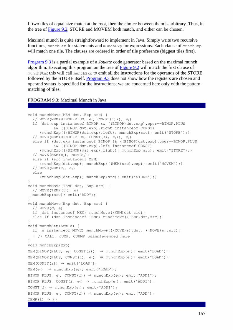
157

If two tiles of equal size match at the root, then the choice between them is arbitrary. Thus, in the tree of Figure 9.2, STORE and MOVEM both match, and either can be chosen.

Maximal munch is quite straightforward to implement in Java. Simply write two recursive functions, munchStm for statements and munchExp for expressions. Each clause of munchExp will match one tile. The clauses are ordered in order of tile preference (biggest tiles first).

Program 9.3 is a partial example of a Jouette code generator based on the maximal munch algorithm. Executing this program on the tree of Figure 9.2 will match the first clause of munchStm; this will call munchExp to emit all the instructions for the operands of the STORE, followed by the STORE itself. Program 9.3 does not show how the registers are chosen and operand syntax is specified for the instructions; we are concerned here only with the pattern-matching of tiles.

PROGRAM 9.3: Maximal Munch in Java. void munchMove(MEM dst, Exp src) { // MOVE(MEM(BINOP(PLUS, e1, CONST(i))), e2) if (dst.exp instanceof BINOP && ((BINOP)dst.exp).oper==BINOP.PLUS && ((BINOP)dst.exp).right instanceof CONST) {munchExp(((BINOP)dst.exp).left); munchExp(src); emit("STORE");} // MOVE(MEM(BINOP(PLUS, CONST(i), e1)), e2) else if (dst.exp instanceof BINOP && ((BINOP)dst.exp).oper==BINOP.PLUS && ((BINOP)dst.exp).left instanceof CONST) {munchExp(((BINOP)dst.exp).right); munchExp(src); emit("STORE");} // MOVE(MEM(e1), MEM(e2)) else if (src instanceof MEM) {munchExp(dst.exp); munchExp(((MEM)src).exp); emit("MOVEM");} // MOVE(MEM(e1, e2) else {munchExp(dst.exp); munchExp(src); emit("STORE");} } void munchMove(TEMP dst, Exp src) { // MOVE(TEMP(t1), e) munchExp(src); emit("ADD"); } void munchMove(Exp dst, Exp src) { // MOVE(d, e) if (dst instanceof MEM) munchMove((MEM)dst,src); else if (dst instanceof TEMP) munchMove((TEMP)dst,src); } void munchStm(Stm s) { if (s instanceof MOVE) munchMove(((MOVE)s).dst, ((MOVE)s).src);

⋮ // CALL, JUMP, CJUMP unimplemented here } void munchExp(Exp)

MEM(BINOP(PLUS, e1, CONST(i))) ⇒ munchExp(e1); emit("LOAD"); MEM(BINOP(PLUS, CONST(i), e1)) ⇒ munchExp(e1); emit("LOAD"); MEM(CONST(i)) ⇒ emit("LOAD"); MEM(e1) ⇒ munchExp(e1); emit("LOAD"); BINOP(PLUS, e1, CONST(i)) ⇒ munchExp(e1); emit("ADDI"); BINOP(PLUS, CONST(i, e1) ⇒ munchExp(e1); emit("ADDI"); CONST(i) ⇒ munchExp(e1); emit("ADDI"); BINOP(PLUS, e1, CONST(i)) ⇒ munchExp(e1); emit("ADD"); TEMP(t) ⇒ {}

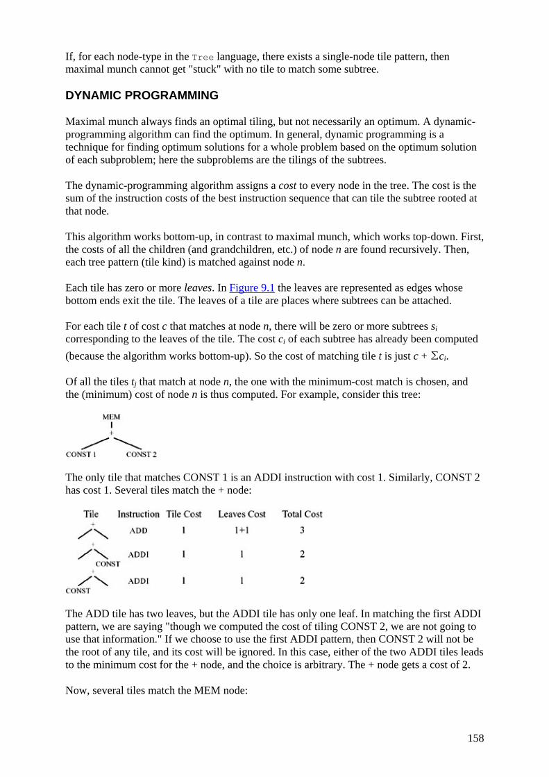
158

If, for each node-type in the Tree language, there exists a single-node tile pattern, then maximal munch cannot get "stuck" with no tile to match some subtree.

DYNAMIC PROGRAMMING

Maximal munch always finds an optimal tiling, but not necessarily an optimum. A dynamic-programming algorithm can find the optimum. In general, dynamic programming is a technique for finding optimum solutions for a whole problem based on the optimum solution of each subproblem; here the subproblems are the tilings of the subtrees.

The dynamic-programming algorithm assigns a cost to every node in the tree. The cost is the sum of the instruction costs of the best instruction sequence that can tile the subtree rooted at that node.

This algorithm works bottom-up, in contrast to maximal munch, which works top-down. First, the costs of all the children (and grandchildren, etc.) of node n are found recursively. Then, each tree pattern (tile kind) is matched against node n.

Each tile has zero or more leaves. In Figure 9.1 the leaves are represented as edges whose bottom ends exit the tile. The leaves of a tile are places where subtrees can be attached.

For each tile t of cost c that matches at node n, there will be zero or more subtrees si corresponding to the leaves of the tile. The cost ci of each subtree has already been computed (because the algorithm works bottom-up). So the cost of matching tile t is just c + ∑ci.

Of all the tiles tj that match at node n, the one with the minimum-cost match is chosen, and the (minimum) cost of node n is thus computed. For example, consider this tree:

The only tile that matches CONST 1 is an ADDI instruction with cost 1. Similarly, CONST 2 has cost 1. Several tiles match the + node:

The ADD tile has two leaves, but the ADDI tile has only one leaf. In matching the first ADDI pattern, we are saying "though we computed the cost of tiling CONST 2, we are not going to use that information." If we choose to use the first ADDI pattern, then CONST 2 will not be the root of any tile, and its cost will be ignored. In this case, either of the two ADDI tiles leads to the minimum cost for the + node, and the choice is arbitrary. The + node gets a cost of 2.

Now, several tiles match the MEM node:

159

Either of the last two matches will be optimum.

Once the cost of the root node (and thus the entire tree) is found, the instruction emission phase begins. The algorithm is as follows:

Emission(node n): for each leaf li of the tile selected at node n, perform Emission(li). Then emit the instruction matched at node n.

Emission(n) does not recur on the children of node n, but on the leaves of the tile that matched at n. For example, after the dynamic-programming algorithm finds the optimum cost of the simple tree above, the emission phase emits

but no instruction is emitted for any tile rooted at the + node, because this was not a leaf of the tile matched at the root.

TREE GRAMMARS

For machines with complex instruction sets and several classes of registers and addressing modes, there is a useful generalization of the dynamic-programming algorithm. Suppose we make a brain-damaged version of Jouette with two classes of registers: a registers for addressing, and d registers for "data." The instruction set of the Schizo-Jouette machine (loosely based on the Motorola 68000) is shown in Figure 9.4.

160

Figure 9.4: The Schizo-Jouette architecture.

The root and leaves of each tile must be marked with a or d to indicate which kind of register is implied. Now, the dynamic-programming algorithm must keep track, for each node, of the min-cost match as an a register, and also the min-cost match as a d register.

At this point it is useful to use a context-free grammar to describe the tiles; the grammar will have nonterminals s (for statements), a (for expressions calculated into an a register), and d (for expressions calculated into a d register). Section 3.1 describes the use of context-free grammars for source-language syntax; here we use them for quite a different purpose.

The grammar rules for the LOAD, MOVEA, and MOVED instructions might look like this:

d → MEM(+(a, CONST)) d → MEM(+(CONST, a)) d → MEM(CONST)

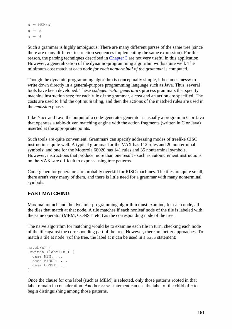
161

d → MEM(a) d → a a → d

Such a grammar is highly ambiguous: There are many different parses of the same tree (since there are many different instruction sequences implementing the same expression). For this reason, the parsing techniques described in Chapter 3 are not very useful in this application. However, a generalization of the dynamic-programming algorithm works quite well: The minimum-cost match at each node for each nonterminal of the grammar is computed.

Though the dynamic-programming algorithm is conceptually simple, it becomes messy to write down directly in a general-purpose programming language such as Java. Thus, several tools have been developed. These codegenerator generators process grammars that specify machine instruction sets; for each rule of the grammar, a cost and an action are specified. The costs are used to find the optimum tiling, and then the actions of the matched rules are used in the emission phase.

Like Yacc and Lex, the output of a code-generator generator is usually a program in C or Java that operates a table-driven matching engine with the action fragments (written in C or Java) inserted at the appropriate points.

Such tools are quite convenient. Grammars can specify addressing modes of treelike CISC instructions quite well. A typical grammar for the VAX has 112 rules and 20 nonterminal symbols; and one for the Motorola 68020 has 141 rules and 35 nonterminal symbols. However, instructions that produce more than one result - such as autoincrement instructions on the VAX -are difficult to express using tree patterns.

Code-generator generators are probably overkill for RISC machines. The tiles are quite small, there aren't very many of them, and there is little need for a grammar with many nonterminal symbols.

FAST MATCHING

Maximal munch and the dynamic-programming algorithm must examine, for each node, all the tiles that match at that node. A tile matches if each nonleaf node of the tile is labeled with the same operator (MEM, CONST, etc.) as the corresponding node of the tree.

The naive algorithm for matching would be to examine each tile in turn, checking each node of the tile against the corresponding part of the tree. However, there are better approaches. To match a tile at node n of the tree, the label at n can be used in a case statement:

match(n) { switch (label(n)) { case MEM: ... case BINOP: ... case CONST: ... }

Once the clause for one label (such as MEM) is selected, only those patterns rooted in that label remain in consideration. Another case statement can use the label of the child of n to begin distinguishing among those patterns.

162

The organization and optimization of decision trees for pattern matching is beyond the scope of this book. However, for better performance the naive sequence of clauses in function munchExp should be rewritten as a sequence of comparisons that never looks twice at the same tree node.

EFFICIENCY OF TILING ALGORITHMS

How expensive are maximal munch and dynamic programming?

Let us suppose that there are T different tiles, and that the average matching tile contains K nonleaf (labeled) nodes. Let K′ be the largest number of nodes that ever need to be examined to see which tiles match at a given subtree; this is approximately the same as the size of the largest tile. And suppose that, on the average, T′ different patterns (tiles) match at each tree node. For a typical RISC machine we might expect T = 50, K = 2, K′ = 4, T′ = 5.

Suppose there are N nodes in the input tree. Then maximal munch will have to consider matches at only N=K nodes because, once a "munch" is made at the root, no pattern-matching needs to take place at the nonleaf nodes of the tile.

To find all the tiles that match at one node, at most K′ tree nodes must be examined; but (with a sophisticated decision tree) each of these nodes will be examined only once. Then each of the successful matches must be compared to see if its cost is minimal. Thus, the matching at each node costs K′ + T′, for a total cost proportional to (K′ + T′)N/K.

The dynamic-programming algorithm must find all the matches at every node, so its cost is proportional to (K′ + T′)N. However, the constant of proportionality is higher than that of maximal munch, since dynamic programming requires two tree-walks instead of one.

Since K, K′, and T′ are constant, the running time of all of these algorithms is linear. In practice, measurements show that these instruction selection algorithms run very quickly compared to the other work performed by a real compiler - even lexical analysis is likely to take more time than instruction selection.

9.2 CISC MACHINES

A typical modern RISC machine has

1. 32 registers, 2. only one class of integer/pointer registers, 3. arithmetic operations only between registers, 4. "three-address" instructions of the form r1 ← r2 ⊕ r3, 5. load and store instructions with only the M[reg+const] addressing mode, 6. every instruction exactly 32 bits long, 7. one result or effect per instruction.

Many machines designed between 1970 and 1985 are complex instruction set computers (CISC). Such computers have more complicated addressing modes that encode instructions in fewer bits, which was important when computer memories were smaller and more expensive. Typical features found on CISC machines include

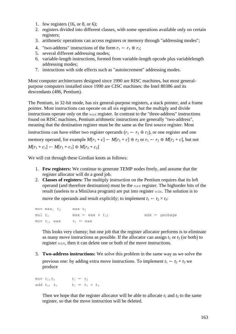
163

1. few registers (16, or 8, or 6); 2. registers divided into different classes, with some operations available only on certain

registers; 3. arithmetic operations can access registers or memory through "addressing modes"; 4. "two-address" instructions of the form r1 ← r1 ⊕ r2; 5. several different addressing modes; 6. variable-length instructions, formed from variable-length opcode plus variablelength

addressing modes; 7. instructions with side effects such as "autoincrement" addressing modes.

Most computer architectures designed since 1990 are RISC machines, but most general-purpose computers installed since 1990 are CISC machines: the Intel 80386 and its descendants (486, Pentium).

The Pentium, in 32-bit mode, has six general-purpose registers, a stack pointer, and a frame pointer. Most instructions can operate on all six registers, but the multiply and divide instructions operate only on the eax register. In contrast to the "three-address" instructions found on RISC machines, Pentium arithmetic instructions are generally "two-address", meaning that the destination register must be the same as the first source register. Most instructions can have either two register operands (r1 ← r1 ⊕ r2), or one register and one memory operand, for example M[r1 + c] ← M[r1 + c] ⊕ r2 or r1 ← r1 ⊕ M[r2 + c], but not M[r1 + c1] ← M[r1 + c1] ⊕ M[r2 + c2]

We will cut through these Gordian knots as follows:

1. Few registers: We continue to generate TEMP nodes freely, and assume that the register allocator will do a good job.

2. Classes of registers: The multiply instruction on the Pentium requires that its left operand (and therefore destination) must be the eax register. The highorder bits of the result (useless to a MiniJava program) are put into register edx. The solution is to move the operands and result explicitly; to implement t1 ← t2 × t3:

mov eax, t2 eax t2

mul t3 eax ← eax × t3; edx ← garbage mov t1, eax t1 ← eax

This looks very clumsy; but one job that the register allocator performs is to eliminate as many move instructions as possible. If the allocator can assign t1 or t3 (or both) to register eax, then it can delete one or both of the move instructions.

3. Two-address instructions: We solve this problem in the same way as we solve the previous one: by adding extra move instructions. To implement t1 ← t2 + t3 we produce

mov t1,t2 t1 ← t2 add t1, t3 t1 ← t1 + t3

Then we hope that the register allocator will be able to allocate t1 and t2 to the same register, so that the move instruction will be deleted.

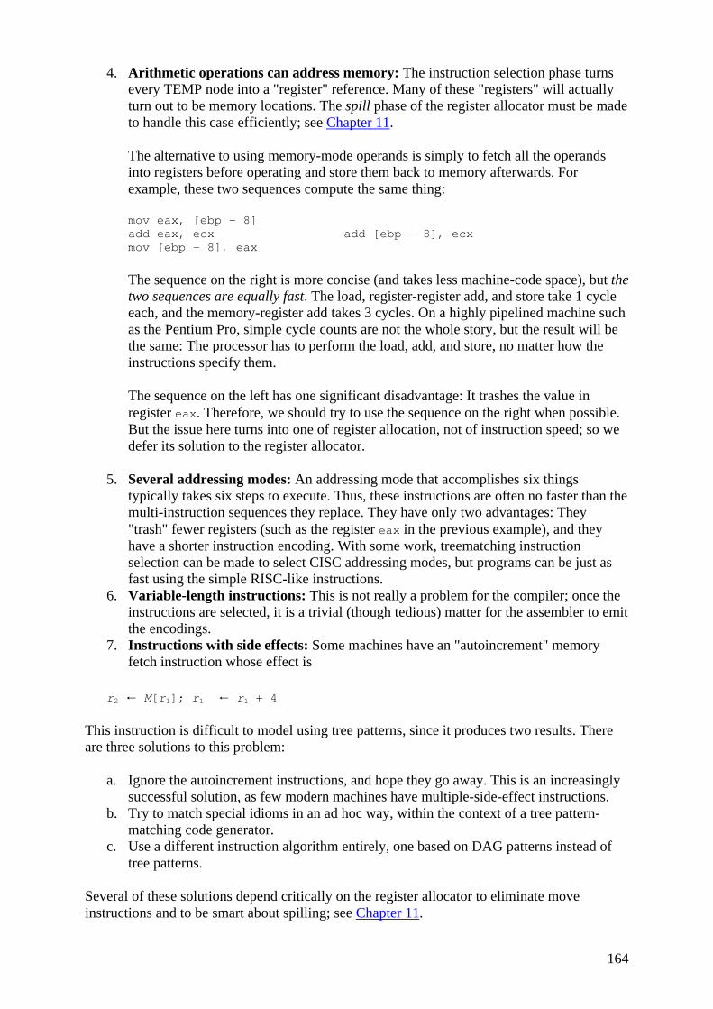
164

4. Arithmetic operations can address memory: The instruction selection phase turns every TEMP node into a "register" reference. Many of these "registers" will actually turn out to be memory locations. The spill phase of the register allocator must be made to handle this case efficiently; see Chapter 11.

The alternative to using memory-mode operands is simply to fetch all the operands into registers before operating and store them back to memory afterwards. For example, these two sequences compute the same thing:

mov eax, [ebp - 8] add eax, ecx add [ebp - 8], ecx mov [ebp - 8], eax

The sequence on the right is more concise (and takes less machine-code space), but the two sequences are equally fast. The load, register-register add, and store take 1 cycle each, and the memory-register add takes 3 cycles. On a highly pipelined machine such as the Pentium Pro, simple cycle counts are not the whole story, but the result will be the same: The processor has to perform the load, add, and store, no matter how the instructions specify them.

The sequence on the left has one significant disadvantage: It trashes the value in register eax. Therefore, we should try to use the sequence on the right when possible. But the issue here turns into one of register allocation, not of instruction speed; so we defer its solution to the register allocator.

5. Several addressing modes: An addressing mode that accomplishes six things typically takes six steps to execute. Thus, these instructions are often no faster than the multi-instruction sequences they replace. They have only two advantages: They "trash" fewer registers (such as the register eax in the previous example), and they have a shorter instruction encoding. With some work, treematching instruction selection can be made to select CISC addressing modes, but programs can be just as fast using the simple RISC-like instructions.

6. Variable-length instructions: This is not really a problem for the compiler; once the instructions are selected, it is a trivial (though tedious) matter for the assembler to emit the encodings.

7. Instructions with side effects: Some machines have an "autoincrement" memory fetch instruction whose effect is

r2 ← M[r1]; r1 ← r1 + 4

This instruction is difficult to model using tree patterns, since it produces two results. There are three solutions to this problem:

a. Ignore the autoincrement instructions, and hope they go away. This is an increasingly successful solution, as few modern machines have multiple-side-effect instructions.

b. Try to match special idioms in an ad hoc way, within the context of a tree pattern-matching code generator.

c. Use a different instruction algorithm entirely, one based on DAG patterns instead of tree patterns.

Several of these solutions depend critically on the register allocator to eliminate move instructions and to be smart about spilling; see Chapter 11.

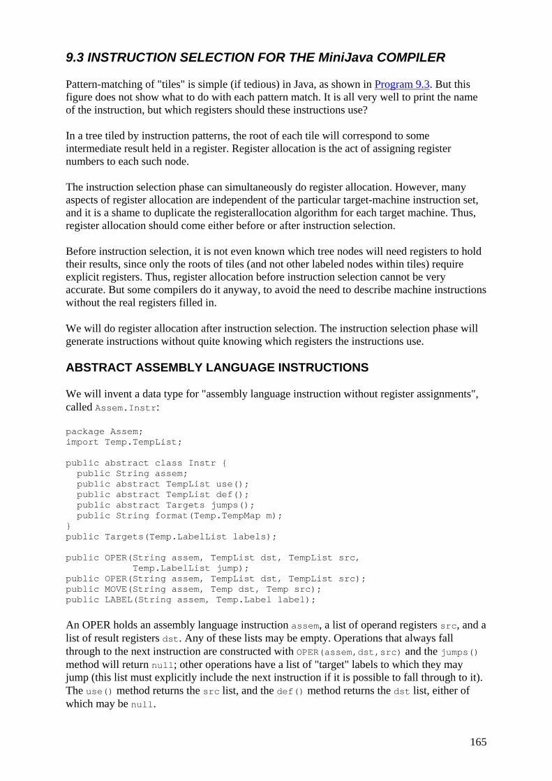
165

9.3 INSTRUCTION SELECTION FOR THE MiniJava COMPILER

Pattern-matching of "tiles" is simple (if tedious) in Java, as shown in Program 9.3. But this figure does not show what to do with each pattern match. It is all very well to print the name of the instruction, but which registers should these instructions use?

In a tree tiled by instruction patterns, the root of each tile will correspond to some intermediate result held in a register. Register allocation is the act of assigning register numbers to each such node.

The instruction selection phase can simultaneously do register allocation. However, many aspects of register allocation are independent of the particular target-machine instruction set, and it is a shame to duplicate the registerallocation algorithm for each target machine. Thus, register allocation should come either before or after instruction selection.

Before instruction selection, it is not even known which tree nodes will need registers to hold their results, since only the roots of tiles (and not other labeled nodes within tiles) require explicit registers. Thus, register allocation before instruction selection cannot be very accurate. But some compilers do it anyway, to avoid the need to describe machine instructions without the real registers filled in.

We will do register allocation after instruction selection. The instruction selection phase will generate instructions without quite knowing which registers the instructions use.

ABSTRACT ASSEMBLY LANGUAGE INSTRUCTIONS

We will invent a data type for "assembly language instruction without register assignments", called Assem.Instr:

package Assem; import Temp.TempList; public abstract class Instr { public String assem; public abstract TempList use(); public abstract TempList def(); public abstract Targets jumps(); public String format(Temp.TempMap m); } public Targets(Temp.LabelList labels); public OPER(String assem, TempList dst, TempList src, Temp.LabelList jump); public OPER(String assem, TempList dst, TempList src); public MOVE(String assem, Temp dst, Temp src); public LABEL(String assem, Temp.Label label);

An OPER holds an assembly language instruction assem, a list of operand registers src, and a list of result registers dst. Any of these lists may be empty. Operations that always fall through to the next instruction are constructed with OPER(assem,dst,src) and the jumps() method will return null; other operations have a list of "target" labels to which they may jump (this list must explicitly include the next instruction if it is possible to fall through to it). The use() method returns the src list, and the def() method returns the dst list, either of which may be null.

166

A LABEL is a point in a program to which jumps may go. It has an assem component showing how the label will look in the assembly language program and a label component identifying which label symbol was used.

A MOVE is like an OPER, but must perform only data transfer. Then, if the dst and src temporaries are assigned to the same register, the MOVE can later be deleted. The use() method returns a singleton list src, and the def() method returns a singleton list dst.

Calling i.format(m) formats an assembly instruction as a string; m is an object implementing the TempMap interface, which contains a method to give the register assignment (or perhaps just the name) of every temp.

package Temp; public interface TempMap { public String tempMap(Temp.Temp t); }

Machine independence. The Assem.Instr class is independent of the chosen target-machine assembly language (though it is tuned for machines with only one class of register). If the target machine is a Sparc, then the assem strings will be Sparc assembly language. We will use Jouette assembly language for illustration.

For example, the tree

could be translated into Jouette assembly language as

new OPER("LOAD 'd0 <- M['s0+8]", new TempList(new Temp(), null), new TempList(frame.FP(), null));

This instruction needs some explanation. The actual assembly language of Jouette, after register allocation, might be

LOAD r1 <- M[r27+8]

assuming that register r27 is the frame pointer fp and that the register allocator decided to assign the new temp to register r1.Butthe Assem instruction does not know about register assignments; instead, it just talks of the sources and destination of each instruction. This LOAD instruction has one source register, which is referred to as ‘s0, and one destination register, referred to as ‘d0.

Another example will be useful. The tree

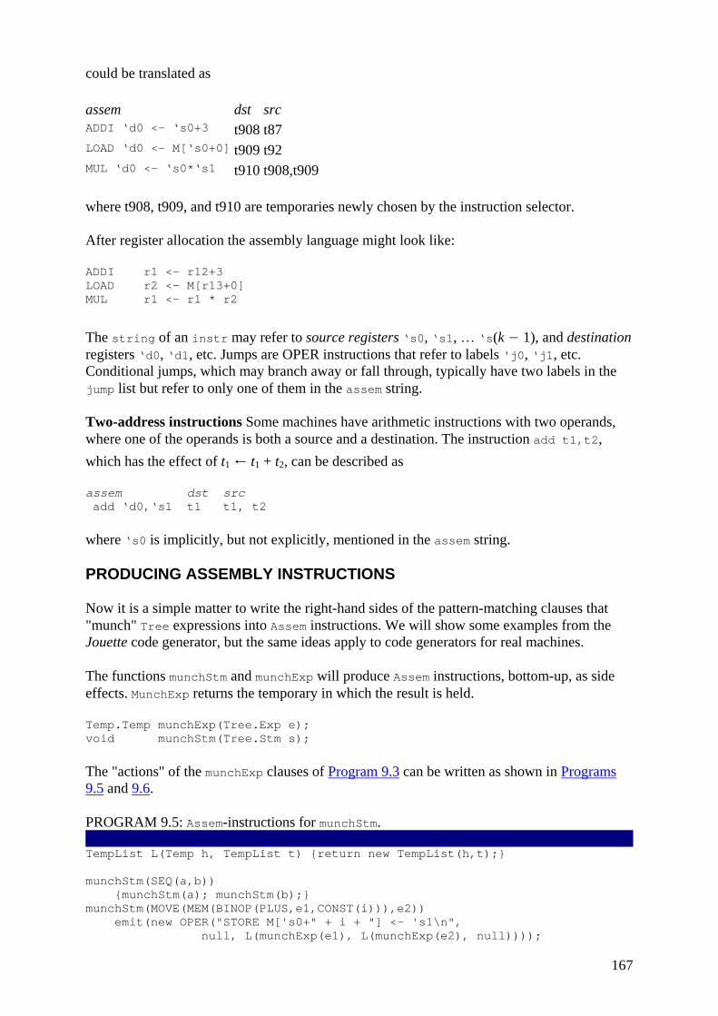
167

could be translated as

assem dst src ADDI ‘d0 <- ‘s0+3 t908 t87 LOAD ‘d0 <- M[‘s0+0] t909 t92 MUL ‘d0 <- ‘s0*‘s1 t910 t908,t909

where t908, t909, and t910 are temporaries newly chosen by the instruction selector.

After register allocation the assembly language might look like:

ADDI r1 <- r12+3 LOAD r2 <- M[r13+0] MUL r1 <- r1 * r2

The string of an instr may refer to source registers ‘s0, ‘s1, … ‘s(k − 1), and destination registers ‘d0, ‘d1, etc. Jumps are OPER instructions that refer to labels ‘j0, ‘j1, etc. Conditional jumps, which may branch away or fall through, typically have two labels in the jump list but refer to only one of them in the assem string.

Two-address instructions Some machines have arithmetic instructions with two operands, where one of the operands is both a source and a destination. The instruction add t1,t2, which has the effect of t1 ← t1 + t2, can be described as

assem dst src add ‘d0,‘s1 t1 t1, t2

where ‘s0 is implicitly, but not explicitly, mentioned in the assem string.

PRODUCING ASSEMBLY INSTRUCTIONS

Now it is a simple matter to write the right-hand sides of the pattern-matching clauses that "munch" Tree expressions into Assem instructions. We will show some examples from the Jouette code generator, but the same ideas apply to code generators for real machines.

The functions munchStm and munchExp will produce Assem instructions, bottom-up, as side effects. MunchExp returns the temporary in which the result is held.

Temp.Temp munchExp(Tree.Exp e); void munchStm(Tree.Stm s);

The "actions" of the munchExp clauses of Program 9.3 can be written as shown in Programs 9.5 and 9.6.

PROGRAM 9.5: Assem-instructions for munchStm. TempList L(Temp h, TempList t) {return new TempList(h,t);} munchStm(SEQ(a,b)) {munchStm(a); munchStm(b);} munchStm(MOVE(MEM(BINOP(PLUS,e1,CONST(i))),e2)) emit(new OPER("STORE M['s0+" + i + "] <- 's1\n", null, L(munchExp(e1), L(munchExp(e2), null))));

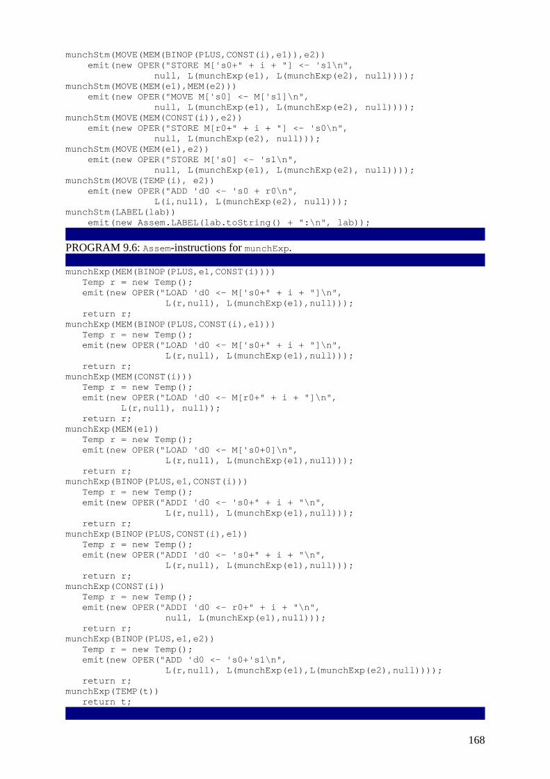
168

munchStm(MOVE(MEM(BINOP(PLUS,CONST(i),e1)),e2)) emit(new OPER("STORE M['s0+" + i + "] <- 's1\n", null, L(munchExp(e1), L(munchExp(e2), null)))); munchStm(MOVE(MEM(e1),MEM(e2))) emit(new OPER("MOVE M['s0] <- M['s1]\n", null, L(munchExp(e1), L(munchExp(e2), null)))); munchStm(MOVE(MEM(CONST(i)),e2)) emit(new OPER("STORE M[r0+" + i + "] <- 's0\n", null, L(munchExp(e2), null))); munchStm(MOVE(MEM(e1),e2)) emit(new OPER("STORE M['s0] <- 's1\n", null, L(munchExp(e1), L(munchExp(e2), null)))); munchStm(MOVE(TEMP(i), e2)) emit(new OPER("ADD 'd0 <- 's0 + r0\n", L(i,null), L(munchExp(e2), null))); munchStm(LABEL(lab)) emit(new Assem.LABEL(lab.toString() + ":\n", lab));

PROGRAM 9.6: Assem-instructions for munchExp. munchExp(MEM(BINOP(PLUS,e1,CONST(i)))) Temp r = new Temp(); emit(new OPER("LOAD 'd0 <- M['s0+" + i + "]\n", L(r,null), L(munchExp(e1),null))); return r; munchExp(MEM(BINOP(PLUS,CONST(i),e1))) Temp r = new Temp(); emit(new OPER("LOAD 'd0 <- M['s0+" + i + "]\n", L(r,null), L(munchExp(e1),null))); return r; munchExp(MEM(CONST(i))) Temp r = new Temp(); emit(new OPER("LOAD 'd0 <- M[r0+" + i + "]\n", L(r,null), null)); return r; munchExp(MEM(e1)) Temp r = new Temp(); emit(new OPER("LOAD 'd0 <- M['s0+0]\n", L(r,null), L(munchExp(e1),null))); return r; munchExp(BINOP(PLUS,e1,CONST(i))) Temp r = new Temp(); emit(new OPER("ADDI 'd0 <- 's0+" + i + "\n", L(r,null), L(munchExp(e1),null))); return r; munchExp(BINOP(PLUS,CONST(i),e1)) Temp r = new Temp(); emit(new OPER("ADDI 'd0 <- 's0+" + i + "\n", L(r,null), L(munchExp(e1),null))); return r; munchExp(CONST(i)) Temp r = new Temp(); emit(new OPER("ADDI 'd0 <- r0+" + i + "\n", null, L(munchExp(e1),null))); return r; munchExp(BINOP(PLUS,e1,e2)) Temp r = new Temp(); emit(new OPER("ADD 'd0 <- 's0+'s1\n", L(r,null), L(munchExp(e1),L(munchExp(e2),null)))); return r; munchExp(TEMP(t)) return t;

169

The emit function just accumulates a list of instructions to be returned later, as shown in Program 9.7.

PROGRAM 9.7: The Codegen class. package Jouette; public class Codegen { Frame frame; public Codegen(Frame f) {frame=f;} private Assem.InstrList ilist=null, last=null; private void emit(Assem.Instr inst) { if (last!=null) last = last.tail = new Assem.InstrList(inst,null); else last = ilist = new Assem.InstrList(inst,null); } void munchStm(Tree.Stm s) { ... } Temp.Temp munchExp(Tree.Exp s) { ... } Assem.InstrList codegen(Tree.Stm s) { Assem.InstrList l; munchStm(s); l=ilist; ilist=last=null; return l; } } package Frame; public class Frame { ... public Assem.InstrList codegen(Tree.Stm stm); { return (new Codegen(this)).codegen(stm); } }

PROCEDURE CALLS

Procedure calls are represented by EXP(CALL(f, args)), and function calls by MOVE(TEMP t, CALL(f, args)). These trees can be matched by tiles such as

munchStm(EXP(CALL(e,args))) {Temp r = munchExp(e); TempList l = munchArgs(0,args); emit(new OPER("CALL 's0\n",calldefs,L(r,l)));}

In this example, munchArgs generates code to move all the arguments to their correct positions, in outgoing parameter registers and/or in memory. The integer parameter to munchArgs is i for the ith argument; munchArgs will recur with i + 1 for the next argument, and so on.

What munchArgs returns is a list of all the temporaries that are to be passed to the machine's CALL instruction. Even though these temps are never written explicitly in assembly language, they should be listed as "sources" of the instruction, so that liveness analysis (Chapter 10) can see that their values need to be kept up to the point of call.

170

A CALL is expected to "trash" certain registers - the caller-save registers, the return-address register, and the return-value register. This list of calldefs should be listed as "destinations" of the CALL, so that the later phases of the compiler know that something happens to them here.

In general, any instruction that has the side effect of writing to another register requires this treatment. For example, the Pentium's multiply instruction writes to register edx with useless high-order result bits, so edx and eax are both listed as destinations of this instruction. (The high-order bits can be very useful for programs written in assembly language to do multiprecision arithmetic, but most programming languages do not support any way to access them.)

IF THERE'S NO FRAME POINTER

In a stack frame layout such as the one shown in Figure 6.2, the frame pointer points at one end of the frame and the stack pointer points at the other. At each procedure call, the stack pointer register is copied to the frame pointer register, and then the stack pointer is incremented by the size of the new frame.

Many machines' calling conventions do not use a frame pointer. Instead, the "virtual frame pointer" is always equal to stack pointer plus frame size. This saves time (no copy instruction) and space (one more register usable for other purposes). But our Translate phase has generated trees that refer to this fictitious frame pointer. The codegen function must replace any reference to FP+k with SP + k + fs, where fs is the frame size. It can recognize these patterns as it munches the trees.

However, to replace them it must know the value of fs, which cannot yet be known because register allocation is not known. Assuming the function f is to be emitted at label L14 (for example), codegen can just put sp+L14_framesize in its assembly instructions and hope that the prologue for f (generated by Frame.procEntryExit3) will include a definition of the assembly language constant L14_framesize. Codegen is passed the frame argument (Program 9.7) so that it can learn the name L14.

Implementations that have a "real" frame pointer won't need this hack and can ignore the frame argument to codegen. But why would an implementation use a real frame pointer when it wastes time and space to do so? The answer is that this permits the frame size to grow and shrink even after it is first created; some languages have permitted dynamic allocation of arrays within the stack frame (e.g., using alloca in C). Calling-convention designers now tend to avoid dynamically adjustable frame sizes, however.

PROGRAM INSTRUCTION SELECTION

Implement the translation to Assem-instructions for your favorite instruction set (let μ stand for Sparc, Mips, Alpha, Pentium, etc.) using maximal munch. If you would like to generate code for a RISC machine, but you have no RISC computer on which to test it, you may wish to use SPIM (a MIPS simulator implemented by James Larus), described on the Web page for this book.

First write the class μ.Codegen implementing the "maximal munch" translation algorithm from IR trees to the Assem data structure.

171

Use the Canon module (described in Chapter 8) to simplify the trees before applying your Codegen module to them. Use the format function to translate the resulting Assem trees to μ assembly language. Since you won't have done register assignment, just pass new Temp.DefaultMap() to format as the translation function from temporaries to strings.

package Temp; public class DefaultMap implements TempMap { public String tempMap(Temp.Temp t) { return t.toString(); } }

This will produce "assembly" language that does not use register names at all: The instructions will use names such as t3, t283, and so on. But some of these temps are the "built-in" ones created by the Frame module to stand for particular machine registers (see page 143), such as Frame.FP. The assembly language will be easier to read if these registers appear with their natural names (e.g., fp instead of t1).

The Frame module must provide a mapping from the special temps to their names, and nonspecial temps to null:

package Frame; public class Frame implements Temp.TempMap {

⋮ abstract public String tempMap(Temp temp); }

Then, for the purposes of displaying your assembly language prior to register allocation, make a new TempMap function that first tries frame.tempMap, and if that returns null, resorts to Temp.toString().

REGISTER LISTS

Make the following lists of registers; for each register, you will need a string for its assembly language representation and a Temp.Temp for referring to it in Tree and Assem data structures.

• specialregs a list of μ registers used to implement "special" registers such as RV and FP and also the stack pointer SP, the return-address register RA, and (on some machines) the zero register ZERO. Some machines may have other special registers;

• argregs a list of μ registers in which to pass outgoing arguments (including the static link);

• calleesaves a list of μ registers that the called procedure (callee) must preserve unchanged (or save and restore);

• callersaves a list of μ registers that the callee may trash.

The four lists of registers must not overlap, and must include any register that might show up in Assem instructions. These lists are not public, but they are useful internally for both Frame and Codegen - for example, to implement munchArgs and to construct the calldefs list.

Implement the procEntryExit2 function of the μ.Frame class.

package Frame;

172

class Frame implements Temp.TempMap {

⋮ abstract public Assem.InstrList procEntryExit2( Assem.InstrList body); }

This function appends a "sink" instruction to the function body to tell the register allocator that certain registers are live at procedure exit. In the case of the Jouette machine, this is simply:

package Jouette; class Frame extends Frame.Frame {

⋮ static TempList returnSink = L(ZERO, L(RA, L(SP, calleeSaves))); static Assem.InstrList append(Assem.InstrList a, Assem.InstrList b) { if (a==null) return b; else {Assem.InstrList p; for(p=a; p.tail!=null; p=p.tail) {} p.tail=b; return a; } } public Assem.InstrList procEntryExit2( Assem.InstrList body) { return append(body, new Assem.InstrList( new Assem.OPER("", null, returnSink),null)); } }

meaning that the temporaries zero, return-address, stack pointer, and all the callee-saves registers are still live at the end of the function. Having zero live at the end means that it is live throughout, which will prevent the register allocator from trying to use it for some other purpose. The same trick works for any other special registers the machine might have.

Files available in $MINIJAVA/chap9 include:

Canon/* Canonicalization and trace generation.

Assem/* The Assem module.

Main/Main.java A Main module that you may wish to adapt.

Your code generator will handle only the body of each procedure or function, but not the procedure entry/exit sequences. Use a "scaffold" version of Frame.procEntryExit3 function:

package μ; class Frame extends Frame.Frame {

⋮ public Frame.Proc procEntryExit3(Assem.InstrList body) { return new Frame.Proc( "PROCEDURE " + name.toString() + "\n", body, "END " + name.toString() + "\n");

173

} }

FURTHER READING

Cattell [1980] expressed machine instructions as tree patterns, invented the maximal munch algorithm for instruction selection, and built a code-generator generator to produce an instruction selection function from a tree-pattern description of an instruction set. Glanville and Graham [1978] expressed the tree patterns as productions in LR(1) grammars, which allows the maximal munch algorithm to use multiple nonterminal symbols to represent different classes of registers and addressing modes. But grammars describing instruction sets are inherently ambiguous, leading to problems with the LR(1) approach; Aho et al. [1989] use dynamic programming to parse the tree grammars, which solves the ambiguity problem, and describe the Twig automatic code-generator generator. The dynamic programming can be done at compiler-construction time instead of code-generation time [Pelegri-Llopart and Graham 1988]; using this technique, the BURG tool [Fraser et al. 1992] has an interface similar to Twig's but generates code much faster.

EXERCISES

• 9.1 For each of the following expressions, draw the tree and generate Jouette-machine instructions using maximal munch. Circle the tiles (as in Figure 9.2), but number them in the order that they are munched, and show the sequence of Jouette instructions that results.

a. MOVE(MEM(+(+(CONST1000, MEM(TEMPx)), TEMPfp)), CONST0) b. BINOP(MUL, CONST5, MEM(CONST100))

• *9.2 Consider a machine with the following instruction: • mult const1(src1), const2(src2), dst3

• r3 ← M[r1 + const1]* M[r2 + const2]

On this machine, r0 is always 0, and M[1] always contains 1.

a. Draw all the tree patterns corresponding to this instruction (and its special cases).

b. Pick one of the bigger patterns and show how to write a Java if-statement to match it, with the Tree representation used for the MiniJava compiler.

• 9.3 The Jouette machine has control-flow instructions as follows:

BRANCHGE if ri ≥ 0 goto LBRANCHLT if ri < 0 goto L BRANCHEQ if ri = 0 goto L BRANCHNE if ri ≠ 0 goto LJUMP goto ri

• where the JUMP instruction goes to an address contained in a register. • Use these instructions to implement the following tree patterns:

• • Assume that a CJUMP is always followed by its false label. Show the best way to

implement each pattern; in some cases you may need to use more than one instruction

174

or make up a new temporary. How do you implement CJUMP(GT, …) without a BRANCHGT instruction?

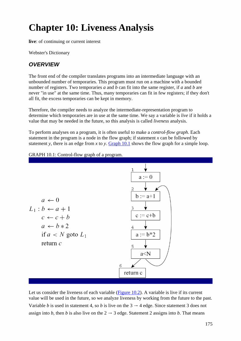
175

Chapter 10: Liveness Analysis live: of continuing or current interest


OVERVIEW

The front end of the compiler translates programs into an intermediate language with an unbounded number of temporaries. This program must run on a machine with a bounded number of registers. Two temporaries a and b can fit into the same register, if a and b are never "in use" at the same time. Thus, many temporaries can fit in few registers; if they don't all fit, the excess temporaries can be kept in memory.

Therefore, the compiler needs to analyze the intermediate-representation program to determine which temporaries are in use at the same time. We say a variable is live if it holds a value that may be needed in the future, so this analysis is called liveness analysis.

To perform analyses on a program, it is often useful to make a control-flow graph. Each statement in the program is a node in the flow graph; if statement x can be followed by statement y, there is an edge from x to y. Graph 10.1 shows the flow graph for a simple loop.

GRAPH 10.1: Control-flow graph of a program.

Let us consider the liveness of each variable (Figure 10.2). A variable is live if its current value will be used in the future, so we analyze liveness by working from the future to the past. Variable b is used in statement 4, so b is live on the 3 → 4 edge. Since statement 3 does not assign into b, then b is also live on the 2 → 3 edge. Statement 2 assigns into b. That means

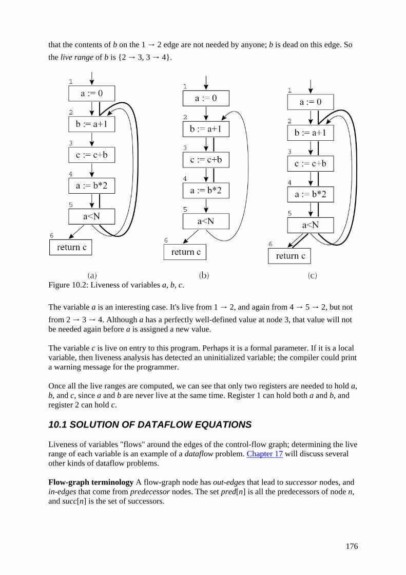
176

that the contents of b on the 1 → 2 edge are not needed by anyone; b is dead on this edge. So the live range of b is {2 → 3, 3 → 4}.

Figure 10.2: Liveness of variables a, b, c.

The variable a is an interesting case. It's live from 1 → 2, and again from 4 → 5 → 2, but not from 2 → 3 → 4. Although a has a perfectly well-defined value at node 3, that value will not be needed again before a is assigned a new value.

The variable c is live on entry to this program. Perhaps it is a formal parameter. If it is a local variable, then liveness analysis has detected an uninitialized variable; the compiler could print a warning message for the programmer.

Once all the live ranges are computed, we can see that only two registers are needed to hold a, b, and c, since a and b are never live at the same time. Register 1 can hold both a and b, and register 2 can hold c.

10.1 SOLUTION OF DATAFLOW EQUATIONS

Liveness of variables "flows" around the edges of the control-flow graph; determining the live range of each variable is an example of a dataflow problem. Chapter 17 will discuss several other kinds of dataflow problems.

Flow-graph terminology A flow-graph node has out-edges that lead to successor nodes, and in-edges that come from predecessor nodes. The set pred[n] is all the predecessors of node n, and succ[n] is the set of successors.

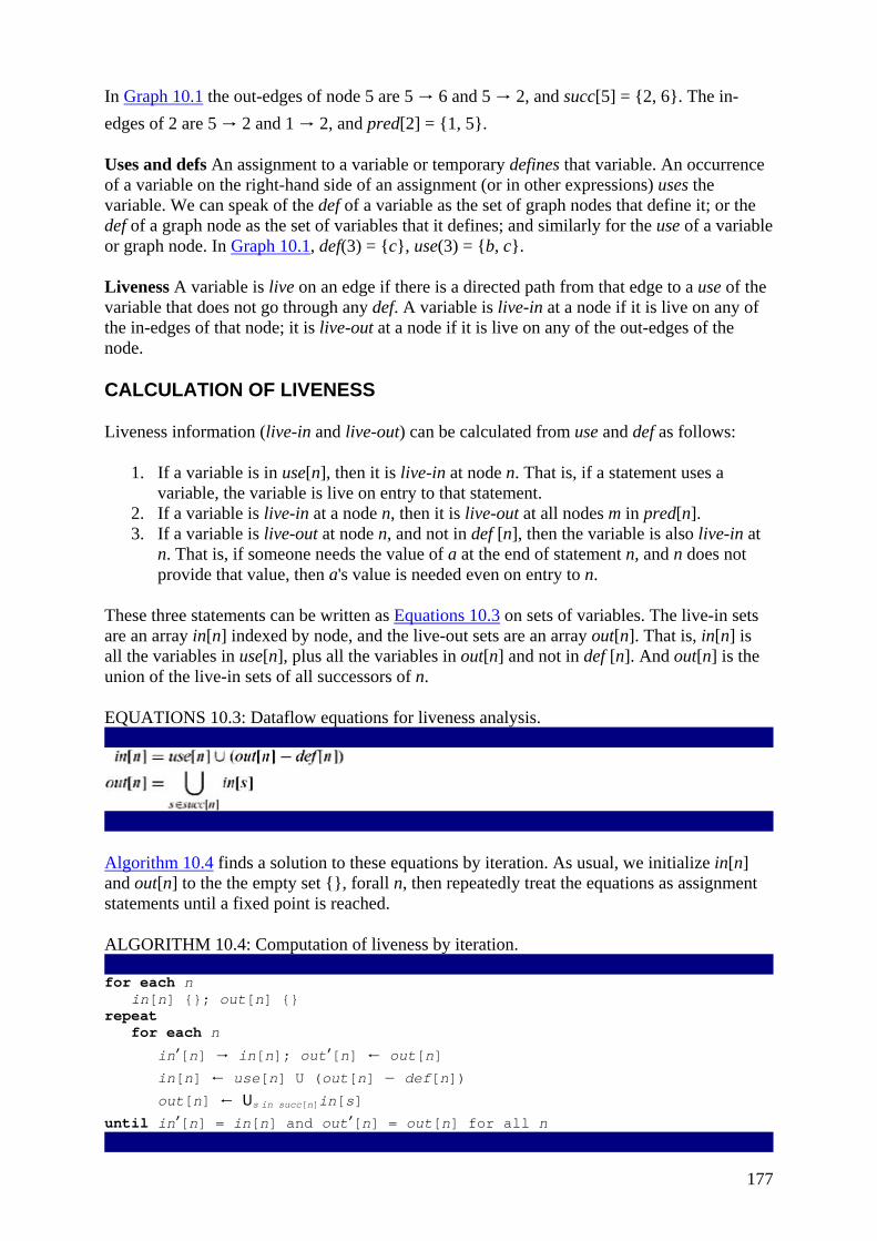
177

In Graph 10.1 the out-edges of node 5 are 5 → 6 and 5 → 2, and succ[5] = {2, 6}. The in-edges of 2 are 5 → 2 and 1 → 2, and pred[2] = {1, 5}.

Uses and defs An assignment to a variable or temporary defines that variable. An occurrence of a variable on the right-hand side of an assignment (or in other expressions) uses the variable. We can speak of the def of a variable as the set of graph nodes that define it; or the def of a graph node as the set of variables that it defines; and similarly for the use of a variable or graph node. In Graph 10.1, def(3) = {c}, use(3) = {b, c}.

Liveness A variable is live on an edge if there is a directed path from that edge to a use of the variable that does not go through any def. A variable is live-in at a node if it is live on any of the in-edges of that node; it is live-out at a node if it is live on any of the out-edges of the node.

CALCULATION OF LIVENESS

Liveness information (live-in and live-out) can be calculated from use and def as follows:

1. If a variable is in use[n], then it is live-in at node n. That is, if a statement uses a variable, the variable is live on entry to that statement.

2. If a variable is live-in at a node n, then it is live-out at all nodes m in pred[n]. 3. If a variable is live-out at node n, and not in def [n], then the variable is also live-in at

n. That is, if someone needs the value of a at the end of statement n, and n does not provide that value, then a's value is needed even on entry to n.

These three statements can be written as Equations 10.3 on sets of variables. The live-in sets are an array in[n] indexed by node, and the live-out sets are an array out[n]. That is, in[n] is all the variables in use[n], plus all the variables in out[n] and not in def [n]. And out[n] is the union of the live-in sets of all successors of n.

EQUATIONS 10.3: Dataflow equations for liveness analysis.

Algorithm 10.4 finds a solution to these equations by iteration. As usual, we initialize in[n] and out[n] to the the empty set {}, forall n, then repeatedly treat the equations as assignment statements until a fixed point is reached.

ALGORITHM 10.4: Computation of liveness by iteration. for each n in[n] {}; out[n] {} repeat for each n

in′[n] → in[n]; out′[n] ← out[n] in[n] ← use[n] U (out[n] − def[n]) out[n] ← Us in succ[n]in[s]

until in′[n] = in[n] and out′[n] = out[n] for all n

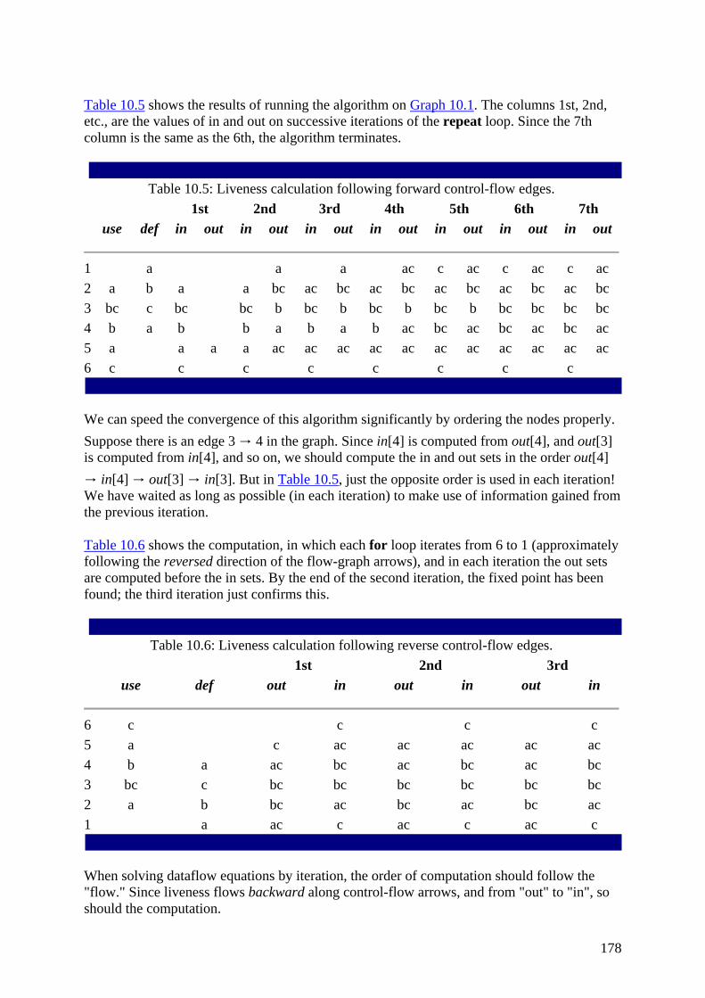
178

Table 10.5 shows the results of running the algorithm on Graph 10.1. The columns 1st, 2nd, etc., are the values of in and out on successive iterations of the repeat loop. Since the 7th column is the same as the 6th, the algorithm terminates.

Table 10.5: Liveness calculation following forward control-flow edges.

1st 2nd 3rd 4th 5th 6th 7th use def in out in out in out in out in out in out in out

1 a a a ac c ac c ac c ac 2 a b a a bc ac bc ac bc ac bc ac bc ac bc 3 bc c bc bc b bc b bc b bc b bc bc bc bc 4 b a b b a b a b ac bc ac bc ac bc ac 5 a a a a ac ac ac ac ac ac ac ac ac ac ac 6 c c c c c c c c

We can speed the convergence of this algorithm significantly by ordering the nodes properly. Suppose there is an edge 3 → 4 in the graph. Since in[4] is computed from out[4], and out[3] is computed from in[4], and so on, we should compute the in and out sets in the order out[4] → in[4] → out[3] → in[3]. But in Table 10.5, just the opposite order is used in each iteration! We have waited as long as possible (in each iteration) to make use of information gained from the previous iteration.

Table 10.6 shows the computation, in which each for loop iterates from 6 to 1 (approximately following the reversed direction of the flow-graph arrows), and in each iteration the out sets are computed before the in sets. By the end of the second iteration, the fixed point has been found; the third iteration just confirms this.

Table 10.6: Liveness calculation following reverse control-flow edges.

1st 2nd 3rd use def out in out in out in

6 c c c c 5 a c ac ac ac ac ac 4 b a ac bc ac bc ac bc 3 bc c bc bc bc bc bc bc 2 a b bc ac bc ac bc ac 1 a ac c ac c ac c

When solving dataflow equations by iteration, the order of computation should follow the "flow." Since liveness flows backward along control-flow arrows, and from "out" to "in", so should the computation.

179

Ordering the nodes can be done easily by depth-first search, as shown in Section 17.4.

Basic blocks Flow-graph nodes that have only one predecessor and one successor are not very interesting. Such nodes can be merged with their predecessors and successors; what results is a graph with many fewer nodes, where each node represents a basic block. The algorithms that operate on flow graphs, such as liveness analysis, go much faster on the smaller graphs. Chapter 17 explains how to adjust the dataflow equations to use basic blocks. In this chapter we keep things simple.

One variable at a time Instead of doing dataflow "in parallel" using set equations, it can be just as practical to compute dataflow for one variable at a time as information about that variable is needed. For liveness, this would mean repeating the dataflow traversal once for each temporary. Starting from each use site of a temporary t, and tracing backward (following predecessor edges of the flow graph) using depth-first search, we note the liveness of t at each flow-graph node. The search stops at any definition of the temporary. Although this might seem expensive, many temporaries have very short live ranges, so the searches terminate quickly and do not traverse the entire flow graph for most variables.

REPRESENTATION OF SETS

There are at least two good ways to represent sets for dataflow equations: as arrays of bits or as sorted lists of variables.

If there are N variables in the program, the bit-array representation uses N bits for each set. Calculating the union of two sets is done by or-ing the corresponding bits at each position. Since computers can represent K bits per word (with K = 32 typical), one set-union operation takes N/K operations.

A set can also be represented as a linked list of its members, sorted by any totally ordered key (such as variable name). Calculating the union is done by merging the lists (discarding duplicates). This takes time proportional to the size of the sets being unioned.

Clearly, when the sets are sparse (fewer than N/K elements, on the average), the sorted-list representation is asymptotically faster; when the sets are dense, the bit-array representation is better.

TIME COMPLEXITY

How fast is iterative dataflow analysis?

A program of size N has at most N nodes in the flow graph, and at most N variables. Thus, each live-in set (or live-out set) has at most N elements; each set-union operation to compute live-in (or live-out) takes O(N) time.

The for loop computes a constant number of set operations per flow-graph node; there are O(N) nodes; thus, the for loop takes O(N2) time.

Each iteration of the repeat loop can only make each in or out set larger, never smaller. This is because the in and out sets are monotonic with respect to each other. That is, in the equation in[n] = use[n]U(out[n]−def[n]), a larger out[n] can only make in[n] larger. Similarly, in out[n] = Us in succ[n]in[s], a larger in[s] can only make out[n] larger.

180

Each iteration must add something to the sets; but the sets cannot keep growing infinitely; at most every set can contain every variable. Thus, the sum of the sizes of all in and out sets is 2N2, which is the most that the repeat loop can iterate.

Thus, the worst-case run time of this algorithm is O(N4). Ordering the nodes using depth-first search (Algorithm 17.5, page 363) usually brings the number of repeat-loop iterations to two or three, and the live sets are often sparse, so the algorithm runs between O(N) and O(N2) in practice.

Section 17.4 discusses more sophisticated ways of solving dataflow equations quickly.

LEAST FIXED POINTS

Table 10.7 illustrates two solutions (and a nonsolution!) to the Equations 10.3; assume there is another program variable d not used in this fragment of the program.

Table 10.7: X and Y are solutions to the liveness equations; Z is not a solution.

X Y Z use def in out in out in out 1 a c ac cd acd c ac 2 a b ac bc acd bcd ac b 3 bc c bc bc bcd bcd b b 4 b a bc ac bcd acd b ac 5 a ac ac acd acd ac ac 6 c c c c

In solution Y, the variable d is carried uselessly around the loop. But in fact, Y satisfies Equations 10.3 just as X does. What does this mean? Is d live or not?

The answer is that any solution to the dataflow equations is a conservative approximation. If the value of variable a will truly be needed in some execution of the program when execution reaches node n of the flow graph, then we can be assured that a is live-out at node n in any solution of the equations. But the converse is not true; we might calculate that d is live-out, but that doesn't mean that its value will really be used.

Is this acceptable? We can answer that question by asking what use will be made of the dataflow information. In the case of liveness analysis, if a variable is thought to be live, then we will make sure to have its value in a register. A conservative approximation of liveness is one that may erroneously believe a variable is live, but will never erroneously believe it is dead. The consequence of a conservative approximation is that the compiled code might use more registers than it really needs; but it will compute the right answer.

Consider instead the live-in sets Z, which fail to satisfy the dataflow equations. Using this Z we think that b and c are never live at the same time, and we would assign them to the same register. The resulting program would use an optimal number of registers but compute the wrong answer.

181

A dataflow equation used for compiler optimization should be set up so that any solution to it provides conservative information to the optimizer; imprecise information may lead to suboptimal but never incorrect programs.

Theorem Equations 10.3 have more than one solution.

Proof X and Y are both solutions.

Theorem All solutions to Equations 10.3 contain solution X. That is, if inX [n] and inY [n] are the live-in sets for some node n in solutions X and Y, then inX [n] ⊆ inY [n].

Proof See Exercise 10.2.

We say that X is the least solution to Equations 10.3. Clearly, since a bigger solution will lead to using more registers (producing suboptimal code), we want to use the least solution. Fortunately, Algorithm 10.4 always computes the least fixed point.

STATIC VS. DYNAMIC LIVENESS

A variable is live "if its value will be used in the future." In Graph 10.8, we know that b × b must be nonnegative, so that the test c ≥ b will be true. Thus, node 4 will never be reached, and a's value will not be used after node 2; a is not live-out of node 2.

GRAPH 10.8: Standard static dataflow analysis will not take advantage of the fact that node 4 can never be reached.

But Equations 10.3 say that a is live-in to node 4, and therefore live-out of nodes 3 and 2. The equations are ignorant of which way the conditional branch will go. "Smarter" equations would permit a and c to be assigned the same register.

Although we can prove here that b*b ≥ 0, and we could have the compiler look for arithmetic identities, no compiler can ever fully understand how all the control flow in every program will work. This is a fundamental mathematical theorem, derivable from the halting problem.

Theorem There is no program H that takes as input any program P and input X and (without infinite-looping) returns true if P(X) halts and false if P(X) infinite-loops.

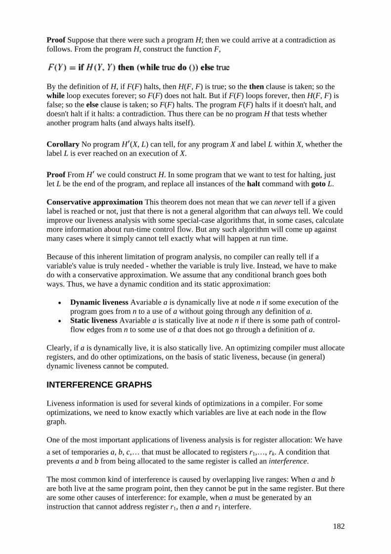
182

Proof Suppose that there were such a program H; then we could arrive at a contradiction as follows. From the program H, construct the function F,

By the definition of H, if F(F) halts, then H(F, F) is true; so the then clause is taken; so the while loop executes forever; so F(F) does not halt. But if F(F) loops forever, then H(F, F) is false; so the else clause is taken; so F(F) halts. The program F(F) halts if it doesn't halt, and doesn't halt if it halts: a contradiction. Thus there can be no program H that tests whether another program halts (and always halts itself).

Corollary No program H′(X, L) can tell, for any program X and label L within X, whether the label L is ever reached on an execution of X.

Proof From H′ we could construct H. In some program that we want to test for halting, just let L be the end of the program, and replace all instances of the halt command with goto L.

Conservative approximation This theorem does not mean that we can never tell if a given label is reached or not, just that there is not a general algorithm that can always tell. We could improve our liveness analysis with some special-case algorithms that, in some cases, calculate more information about run-time control flow. But any such algorithm will come up against many cases where it simply cannot tell exactly what will happen at run time.

Because of this inherent limitation of program analysis, no compiler can really tell if a variable's value is truly needed - whether the variable is truly live. Instead, we have to make do with a conservative approximation. We assume that any conditional branch goes both ways. Thus, we have a dynamic condition and its static approximation:

• Dynamic liveness Avariable a is dynamically live at node n if some execution of the program goes from n to a use of a without going through any definition of a.

• Static liveness Avariable a is statically live at node n if there is some path of control-flow edges from n to some use of a that does not go through a definition of a.

Clearly, if a is dynamically live, it is also statically live. An optimizing compiler must allocate registers, and do other optimizations, on the basis of static liveness, because (in general) dynamic liveness cannot be computed.

INTERFERENCE GRAPHS

Liveness information is used for several kinds of optimizations in a compiler. For some optimizations, we need to know exactly which variables are live at each node in the flow graph.

One of the most important applications of liveness analysis is for register allocation: We have a set of temporaries a, b, c,… that must be allocated to registers r1,…, rk. A condition that prevents a and b from being allocated to the same register is called an interference.

The most common kind of interference is caused by overlapping live ranges: When a and b are both live at the same program point, then they cannot be put in the same register. But there are some other causes of interference: for example, when a must be generated by an instruction that cannot address register r1, then a and r1 interfere.

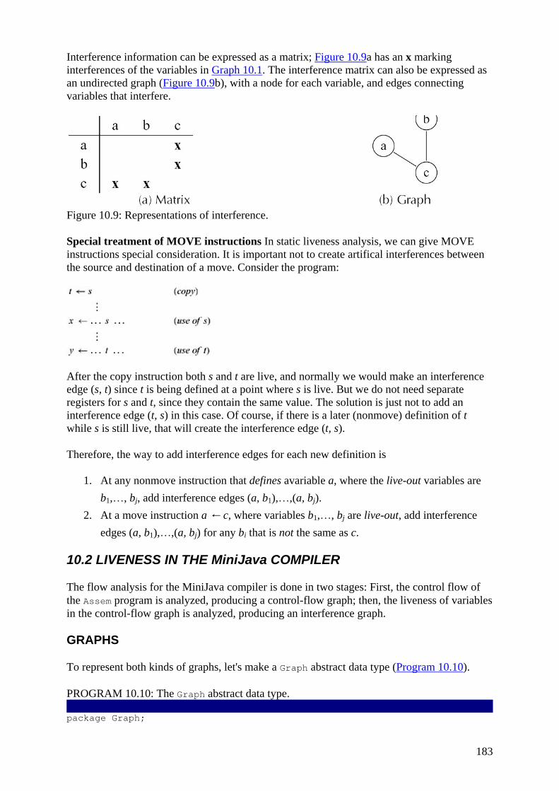
183

Interference information can be expressed as a matrix; Figure 10.9a has an x marking interferences of the variables in Graph 10.1. The interference matrix can also be expressed as an undirected graph (Figure 10.9b), with a node for each variable, and edges connecting variables that interfere.

Figure 10.9: Representations of interference.

Special treatment of MOVE instructions In static liveness analysis, we can give MOVE instructions special consideration. It is important not to create artifical interferences between the source and destination of a move. Consider the program:

After the copy instruction both s and t are live, and normally we would make an interference edge (s, t) since t is being defined at a point where s is live. But we do not need separate registers for s and t, since they contain the same value. The solution is just not to add an interference edge (t, s) in this case. Of course, if there is a later (nonmove) definition of t while s is still live, that will create the interference edge (t, s).

Therefore, the way to add interference edges for each new definition is

1. At any nonmove instruction that defines avariable a, where the live-out variables are b1,…, bj, add interference edges (a, b1),…,(a, bj).

2. At a move instruction a ← c, where variables b1,…, bj are live-out, add interference edges (a, b1),…,(a, bj) for any bi that is not the same as c.

10.2 LIVENESS IN THE MiniJava COMPILER

The flow analysis for the MiniJava compiler is done in two stages: First, the control flow of the Assem program is analyzed, producing a control-flow graph; then, the liveness of variables in the control-flow graph is analyzed, producing an interference graph.

GRAPHS

To represent both kinds of graphs, let's make a Graph abstract data type (Program 10.10).

PROGRAM 10.10: The Graph abstract data type. package Graph;

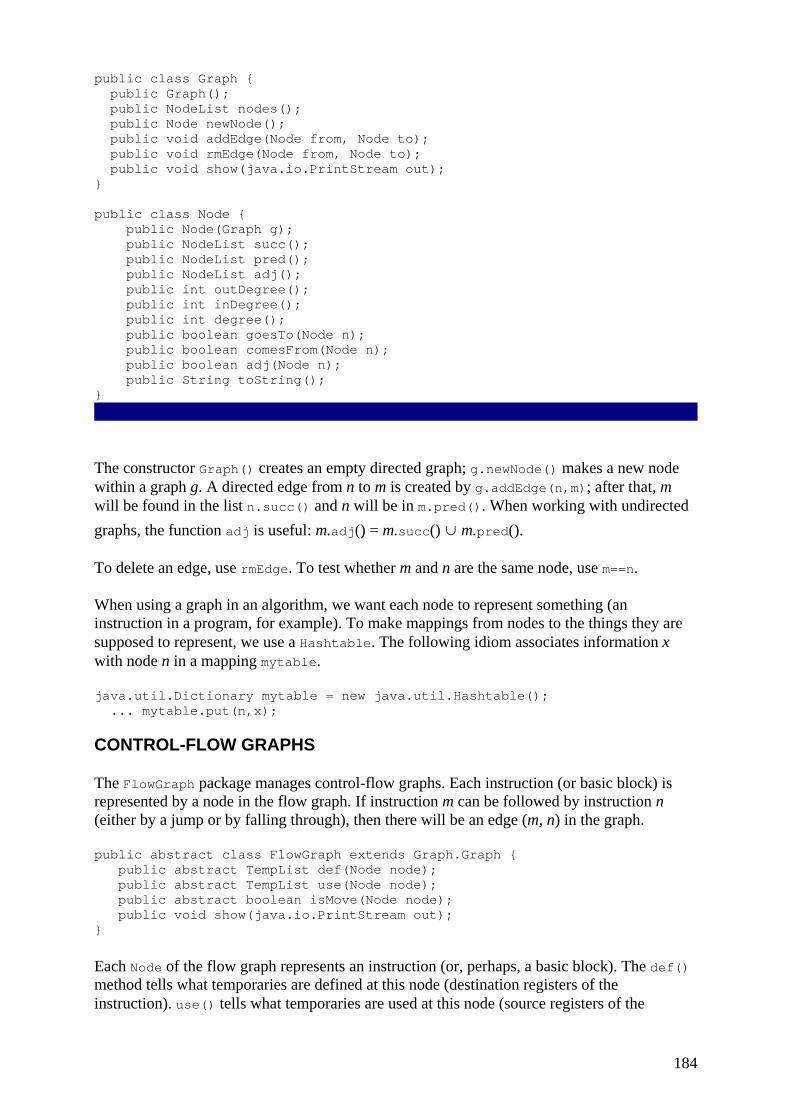
184

public class Graph { public Graph(); public NodeList nodes(); public Node newNode(); public void addEdge(Node from, Node to); public void rmEdge(Node from, Node to); public void show(java.io.PrintStream out); } public class Node { public Node(Graph g); public NodeList succ(); public NodeList pred(); public NodeList adj(); public int outDegree(); public int inDegree(); public int degree(); public boolean goesTo(Node n); public boolean comesFrom(Node n); public boolean adj(Node n); public String toString(); }

The constructor Graph() creates an empty directed graph; g.newNode() makes a new node within a graph g. A directed edge from n to m is created by g.addEdge(n,m); after that, m will be found in the list n.succ() and n will be in m.pred(). When working with undirected graphs, the function adj is useful: m.adj() = m.succ() ∪ m.pred().

To delete an edge, use rmEdge. To test whether m and n are the same node, use m==n.

When using a graph in an algorithm, we want each node to represent something (an instruction in a program, for example). To make mappings from nodes to the things they are supposed to represent, we use a Hashtable. The following idiom associates information x with node n in a mapping mytable.

java.util.Dictionary mytable = new java.util.Hashtable(); ... mytable.put(n,x);

CONTROL-FLOW GRAPHS

The FlowGraph package manages control-flow graphs. Each instruction (or basic block) is represented by a node in the flow graph. If instruction m can be followed by instruction n (either by a jump or by falling through), then there will be an edge (m, n) in the graph.

public abstract class FlowGraph extends Graph.Graph { public abstract TempList def(Node node); public abstract TempList use(Node node); public abstract boolean isMove(Node node); public void show(java.io.PrintStream out); }

Each Node of the flow graph represents an instruction (or, perhaps, a basic block). The def() method tells what temporaries are defined at this node (destination registers of the instruction). use() tells what temporaries are used at this node (source registers of the

185

instruction). isMove tells whether this instruction is a MOVE instruction, one that could be deleted if the def and use were identical.

The AssemFlowGraph class provides an implementation of FlowGraph for Assem instructions.

package FlowGraph; public class AssemFlowGraph extends FlowGraph { public Instr instr(Node n); public AssemFlowGraph(Assem.InstrList instrs); }

The constructor AssemFlowGraph takes a list of instructions and returns a flow graph. In making the flow graph, the jump fields of the instrs are used in creating control-flow edges, and the use and def information (obtained from the src and dst fields of the instrs) is attached to the nodes by means of the use and def methods of the flowgraph.

Information associated with the nodes For a flow graph, we want to associate some use and def information with each node in the graph. Then the liveness-analysis algorithm will also want to remember live-in and live-out information at each node. We could make room in the Node class to store all of this information. This would work well and would be quite efficient. However, it may not be very modular. Eventually we may want to do other analyses on flow graphs, which remember other kinds of information about each node. We may not want to modify the data structure (which is a widely used interface) for each new analysis.

Instead of storing the information in the nodes, a more modular approach is to say that a graph is a graph, and that a flow graph is a graph along with separately packaged auxiliary information (tables, or functions mapping nodes to whatever). Similarly, a dataflow algorithm on a graph does not need to modify dataflow information in the nodes, but modifies its own privately held mappings.

There may be a trade-off here between efficiency and modularity, since it may be faster to keep the information in the nodes, accessible by a simple pointer-traversal instead of a hash-table or search-tree lookup.

LIVENESS ANALYSIS

The RegAlloc package has an abstract class InterferenceGraph to indicate which pairs of temporaries cannot share a register:

package RegAlloc; abstract public class InterferenceGraph extends Graph.Graph{ abstract public Graph.Node tnode(Temp.Temp temp); abstract public Temp.Temp gtemp(Node node); abstract public MoveList moves(); public int spillCost(Node node); }

The method tnode relates a Temp to a Node, and gtemp is the inverse map. The method moves tells what MOVE instructions are associated with this graph (this is a hint about what pairs of temporaries to try to allocate to the same register). The spillCost(n) is an estimate of how many extra instructions would be executed if n were kept in memory instead of in registers; for a naive spiller, it suffices to return 1 for every n.

The class Liveness produces an interference graph from a flow graph:

186

package RegAlloc; public class Liveness extends InterferenceGraph { public Liveness(FlowGraph flow); }

In the implementation of the Liveness module, it is useful to maintain a data structure that remembers what is live at the exit of each flow-graph node:

private java.util.Dictionary liveMap = new java.util.Hashtable();

where the keys are nodes and objects are TempLists. Given a flow-graph node n, the set of live temporaries at that node can be looked up in a global liveMap.

Having calculated a complete liveMap, we can now construct an interference graph. At each flow node n where there is a newly defined temporary d ∈ def(n), and where temporaries {t1, t2;…} are in the liveMap, we just add interference edges (d, t1), (d, t2),…. For MOVEs, these edges will be safe but suboptimal; pages 213-214 describe a better treatment.

What if a newly defined temporary is not live just after its definition? This would be the case if a variable is defined but never used. It would seem that there's no need to put it in a register at all; thus it would not interfere with any other temporaries. But if the defining instruction is going to execute (perhaps it is necessary for some other side effect of the instruction), then it will write to some register, and that register had better not contain any other live variable. Thus, zero-length live ranges do interfere with any live ranges that overlap them.

PROGRAM CONSTRUCTING FLOW GRAPHS

Implement the AssemFlowGraph class that turns a list of Assem instructions into a flow graph. Use the abstract classes Graph.Graph and Flow- Graph.FlowGraph provided in $MINIJAVA/chap10.

PROGRAM LIVENESS

Implement the Liveness module. Use either the set-equation algorithm with the array-of-boolean or sorted-list-of-temporaries representation of sets, or the one-variable-at-a-time method.

EXERCISES

• 10.1 Perform flow analysis on the program of Exercise 8.6: a. Draw the control-flow graph. b. Calculate live-in and live-out at each statement. c. Construct the register interference graph.

• **10.2 Prove that Equations 10.3 have a least fixed point and that Algorithm 10.4 always computes it.

Hint: We know the algorithm refuses to terminate until it has a fixed point. The questions are whether (a) it must eventually terminate, and (b) the fixed point it computes is smaller than all other fixed points. For (a) show that the sets can only get bigger. For (b) show by induction that at any time the in and out sets are subsets of

187

those in any possible fixed point. This is clearly true initially, when in and out are both empty; show that each step of the algorithm preserves the invariant.

• *10.3 Analyze the asymptotic complexity of the one-variable-at-a-time method of computing dataflow information.

• *10.4 Analyze the worst-case asymptotic complexity of making an interference graph, for a program of size N (with at most N variables and at most N control-flow nodes). Assume the dataflow analysis is already done and that use, def, and live-out information for each node can be queried in constant time. What representation of graph adjacency matrices should be used for efficiency?

• 10.5 The DEC Alpha architecture places the following restrictions on floating-point instructions, for programs that wish to recover from arithmetic exceptions:

1. Within a basic block (actually, in any sequence of instructions not separated by a trap-barrier instruction), no two instructions should write to the same destination register. 2. A source register of an instruction cannot be the same as the destination register of that instruction or any later instruction in the basic block.

r1 + r5 → r4 r1 + r5 → r4 r1 + r5 → r3 r1 + r5 → r4

r3 × r2 → r4 r4 × r2 → r1 r4 × r2 → r4 r4 × r2 → r6 violates rule 1. violates rule 2. violates rule 2. OK

3. Show how to express these restrictions in the register interference graph.

188

Chapter 11: Register Allocation reg-is-ter: a device for storing small amounts of data al-lo-cate: to apportion for a specific purpose


OVERVIEW

The Translate, Canon, and Codegen phases of the compiler assume that there are an infinite number of registers to hold temporary values and that MOVE instructions cost nothing. The job of the register allocator is to assign the many temporaries to a small number of machine registers, and, where possible, to assign the source and destination of a MOVE to the same register so that the MOVE can be deleted.

From an examination of the control and dataflow graph, we derive an interference graph. Each node in the interference graph represents a temporary value; each edge (t1, t2) indicates a pair of temporaries that cannot be assigned to the same register. The most common reason for an interference edge is that t1 and t2 are live at the same time. Interference edges can also express other constraints; for example, if a certain instruction a ← b ⊕ c cannot produce results in register r12 on our machine, we can make a interfere with r12.

Next we color the interference graph. We want to use as few colors as possible, but no pair of nodes connected by an edge may be assigned the same color. Graph coloring problems derive from the old mapmakers' rule that adjacent countries on a map should be colored with different colors. Our "colors" correspond to registers: If our target machine has K registers, and we can K -color the graph (color the graph with K colors), then the coloring is a valid register assignment for the interference graph. If there is no K -coloring, we will have to keep some of our variables and temporaries in memory instead of registers; this is called spilling.

11.1 COLORING BY SIMPLIFICATION

Register allocation is an NP-complete problem (except in special cases, such as expression trees); graph coloring is also NP-complete. Fortunately there is a linear-time approximation algorithm that gives good results; its principal phases are Build, Simplify, Spill, and Select.

Build: Construct the interference graph. We use dataflow analysis to compute the set of temporaries that are simultaneously live at each program point, and we add an edge to the graph for each pair of temporaries in the set. We repeat this for all program points.

Simplify: We color the graph using a simple heuristic. Suppose the graph G contains a node m with fewer than K neighbors, where K is the number of registers on the machine. Let G′ be the graph G − {m} obtained by removing m. If G′ can be colored, then so can G, for when m is added to the colored graph G′, the neighbors of m have at most K − 1 colors among them, so a free color can always be found for m. This leads naturally to a stack-based (or recursive) algorithm for coloring: We repeatedly remove (and push on a stack) nodes of degree less than K. Each such simplification will decrease the degrees of other nodes, leading to more opportunity for simplification.

189

Spill: Suppose at some point during simplification the graph G has nodes only of significant degree, that is, nodes of degree ≥ K . Then the simplify heuristic fails, and we mark some node for spilling. That is, we choose some node in the graph (standing for a temporary variable in the program) and decide to represent it in memory, not registers, during program execution. An optimistic approximation to the effect of spilling is that the spilled node does not interfere with any of the other nodes remaining in the graph. It can therefore be removed and pushed on the stack, and the simplify process continued.

Select: We assign colors to nodes in the graph. Starting with the empty graph, we rebuild the original graph by repeatedly adding a node from the top of the stack. When we add a node to the graph, there must be a color for it, as the premise for removing it in the simplify phase was that it could always be assigned a color provided the remaining nodes in the graph could be successfully colored.

When potential spill node n that was pushed using the Spill heuristic is popped, there is no guarantee that it will be colorable: Its neighbors in the graph may be colored with K different colors already. In this case, we have an actual spill. We do not assign any color, but we continue the Select phase to identify other actual spills.

But perhaps some of the neighbors are the same color, so that among them there are fewer than K colors. Then we can color n, and it does not become an actual spill. This technique is known as optimistic coloring.

Start over: If the Select phase is unable to find a color for some node(s), then the program must be rewritten to fetch them from memory just before each use, and store them back after each definition. Thus, a spilled temporary will turn into several new temporaries with tiny live ranges. These will interfere with other temporaries in the graph. So the algorithm is repeated on this rewritten program. This process iterates until simplify succeeds with no spills; in practice, one or two iterations almost always suffice.

EXAMPLE

Graph 11.1 shows the interferences for a simple program. The nodes are labeled with the temporaries they represent, and there is an edge between two nodes if they are simultaneously live. For example, nodes d, k, and j are all connected since they are live simultaneously at the end of the block. Assuming that there are four registers available on the machine, then the simplify phase can start with the nodes g, h, c, and f in its working set, since they have less than four neighbors each. A color can always be found for them if the remaining graph can be successfully colored. If the algorithm starts by removing h and g and all their edges, then node k becomes a candidate for removal and can be added to the work list. Graph 11.2 remains after nodes g, h, and k have been removed. Continuing in this fashion a possible order in which nodes are removed is represented by the stack shown in Figure 11.3a, where the stack grows upward.

GRAPH 11.1: Interference graph for a program. Dotted lines are not interference edges but indicate move instructions.

190

GRAPH 11.2: After removal of h, g, k.

Figure 11.3: Simplification stack, and a possible coloring.

The nodes are now popped off the stack and the original graph reconstructed and colored simultaneously. Starting with m, a color is chosen arbitrarily since the graph at this point consists of a singleton node. The next node to be put into the graph is c. The only constraint is that it be given a color different from m, since there is an edge from m to c. A possible assignment of colors for the reconstructed original graph is shown in Figure 11.3b.

191

11.2 COALESCING

It is easy to eliminate redundant move instructions with an interference graph. If there is no edge in the interference graph between the source and destination of a move instruction, then the move can be eliminated. The source and destination nodes are coalesced into a new node whose edges are the union of those of the nodes being replaced.

In principle, any pair of nodes not connected by an interference edge could be coalesced. This aggressive form of copy propagation is very successful at eliminating move instructions. Unfortunately, the node being introduced is more constrained than those being removed, as it contains a union of edges. Thus, it is quite possible that a graph, colorable with K colors before coalescing, may no longer be K -colorable after reckless coalescing. We wish to coalesce only where it is safe to do so, that is, where the coalescing will not render the graph uncolorable. Both of the following strategies are safe:

Briggs: Nodes a and b can be coalesced if the resulting node ab will have fewer than K neighbors of significant degree (i.e., having ≥ K edges). The coalescing is guaranteed not to turn a K -colorable graph into a non-K -colorable graph, because after the simplify phase has removed all the insignificantdegree nodes from the graph, the coalesced node will be adjacent only to those neighbors that were of significant degree. Since there are fewer than K of these, simplify can then remove the coalesced node from the graph. Thus if the original graph was colorable, the conservative coalescing strategy does not alter the colorability of the graph.

George: Nodes a and b can be coalesced if, for every neighbor t of a, either t already interferes with b or t is of insignificant degree. This coalescing is safe, by the following reasoning. Let S be the set of insignificant-degree neighbors of a in the original graph. If the coalescing were not done, simplify could remove all the nodes in S, leaving a reduced graph G1. If the coalescing is done, then simplify can remove all the nodes in S, leaving a graph G2. But G2 is a subgraph of G1 (the node ab in G2 corresponds to the node b in G1), and thus must be at least as easy to color.

These strategies are conservative, because there are still safe situations in which they will fail to coalesce. This means that the program may perform some unnecessary MOVE instructions - but this is better than spilling!

Interleaving simplification steps with conservative coalescing eliminates most move instructions, while still guaranteeing not to introduce spills. The coalesce, simplify, and spill procedures should be alternated until the graph is empty, as shown in Figure 11.4.

Figure 11.4: Graph coloring with coalescing.

These are the phases of a register allocator with coalescing:

Build: Construct the interference graph, and categorize each node as either move-related or non-move-related. A move-related node is one that is either the source or destination of a move instruction.

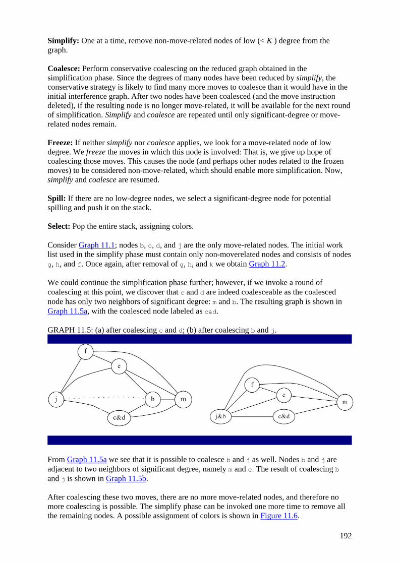
192

Simplify: One at a time, remove non-move-related nodes of low (< K ) degree from the graph.

Coalesce: Perform conservative coalescing on the reduced graph obtained in the simplification phase. Since the degrees of many nodes have been reduced by simplify, the conservative strategy is likely to find many more moves to coalesce than it would have in the initial interference graph. After two nodes have been coalesced (and the move instruction deleted), if the resulting node is no longer move-related, it will be available for the next round of simplification. Simplify and coalesce are repeated until only significant-degree or move-related nodes remain.

Freeze: If neither simplify nor coalesce applies, we look for a move-related node of low degree. We freeze the moves in which this node is involved: That is, we give up hope of coalescing those moves. This causes the node (and perhaps other nodes related to the frozen moves) to be considered non-move-related, which should enable more simplification. Now, simplify and coalesce are resumed.

Spill: If there are no low-degree nodes, we select a significant-degree node for potential spilling and push it on the stack.

Select: Pop the entire stack, assigning colors.

Consider Graph 11.1; nodes b, c, d, and j are the only move-related nodes. The initial work list used in the simplify phase must contain only non-moverelated nodes and consists of nodes g, h, and f. Once again, after removal of g, h, and k we obtain Graph 11.2.

We could continue the simplification phase further; however, if we invoke a round of coalescing at this point, we discover that c and d are indeed coalesceable as the coalesced node has only two neighbors of significant degree: m and b. The resulting graph is shown in Graph 11.5a, with the coalesced node labeled as c&d.

GRAPH 11.5: (a) after coalescing c and d; (b) after coalescing b and j.

From Graph 11.5a we see that it is possible to coalesce b and j as well. Nodes b and j are adjacent to two neighbors of significant degree, namely m and e. The result of coalescing b and j is shown in Graph 11.5b.

After coalescing these two moves, there are no more move-related nodes, and therefore no more coalescing is possible. The simplify phase can be invoked one more time to remove all the remaining nodes. A possible assignment of colors is shown in Figure 11.6.

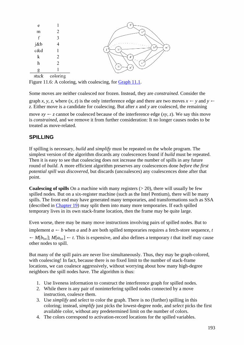
193

Figure 11.6: A coloring, with coalescing, for Graph 11.1.

Some moves are neither coalesced nor frozen. Instead, they are constrained. Consider the graph x, y, z, where (x, z) is the only interference edge and there are two moves x ← y and y ← z. Either move is a candidate for coalescing. But after x and y are coalesced, the remaining move xy ← z cannot be coalesced because of the interference edge (xy, z). We say this move is constrained, and we remove it from further consideration: It no longer causes nodes to be treated as move-related.

SPILLING

If spilling is necessary, build and simplify must be repeated on the whole program. The simplest version of the algorithm discards any coalescences found if build must be repeated. Then it is easy to see that coalescing does not increase the number of spills in any future round of build. A more efficient algorithm preserves any coalescences done before the first potential spill was discovered, but discards (uncoalesces) any coalescences done after that point.

Coalescing of spills On a machine with many registers (> 20), there will usually be few spilled nodes. But on a six-register machine (such as the Intel Pentium), there will be many spills. The front end may have generated many temporaries, and transformations such as SSA (described in Chapter 19) may split them into many more temporaries. If each spilled temporary lives in its own stack-frame location, then the frame may be quite large.

Even worse, there may be many move instructions involving pairs of spilled nodes. But to implement a ← b when a and b are both spilled temporaries requires a fetch-store sequence, t ← M[bloc]; M[aloc] ← t. This is expensive, and also defines a temporary t that itself may cause other nodes to spill.

But many of the spill pairs are never live simultaneously. Thus, they may be graph-colored, with coalescing! In fact, because there is no fixed limit to the number of stack-frame locations, we can coalesce aggressively, without worrying about how many high-degree neighbors the spill nodes have. The algorithm is thus:

1. Use liveness information to construct the interference graph for spilled nodes. 2. While there is any pair of noninterfering spilled nodes connected by a move

instruction, coalesce them. 3. Use simplify and select to color the graph. There is no (further) spilling in this

coloring; instead, simplify just picks the lowest-degree node, and select picks the first available color, without any predetermined limit on the number of colors.

4. The colors correspond to activation-record locations for the spilled variables.

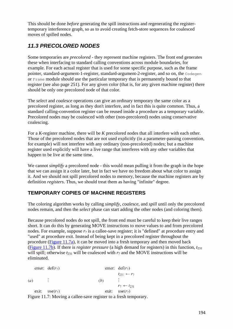
194

This should be done before generating the spill instructions and regenerating the register-temporary interference graph, so as to avoid creating fetch-store sequences for coalesced moves of spilled nodes.

11.3 PRECOLORED NODES

Some temporaries are precolored - they represent machine registers. The front end generates these when interfacing to standard calling conventions across module boundaries, for example. For each actual register that is used for some specific purpose, such as the frame pointer, standard-argument-1-register, standard-argument-2-register, and so on, the Codegen or Frame module should use the particular temporary that is permanently bound to that register (see also page 251). For any given color (that is, for any given machine register) there should be only one precolored node of that color.

The select and coalesce operations can give an ordinary temporary the same color as a precolored register, as long as they don't interfere, and in fact this is quite common. Thus, a standard calling-convention register can be reused inside a procedure as a temporary variable. Precolored nodes may be coalesced with other (non-precolored) nodes using conservative coalescing.

For a K-register machine, there will be K precolored nodes that all interfere with each other. Those of the precolored nodes that are not used explicitly (in a parameter-passing convention, for example) will not interfere with any ordinary (non-precolored) nodes; but a machine register used explicitly will have a live range that interferes with any other variables that happen to be live at the same time.

We cannot simplify a precolored node - this would mean pulling it from the graph in the hope that we can assign it a color later, but in fact we have no freedom about what color to assign it. And we should not spill precolored nodes to memory, because the machine registers are by definition registers. Thus, we should treat them as having "infinite" degree.

TEMPORARY COPIES OF MACHINE REGISTERS

The coloring algorithm works by calling simplify, coalesce, and spill until only the precolored nodes remain, and then the select phase can start adding the other nodes (and coloring them).

Because precolored nodes do not spill, the front end must be careful to keep their live ranges short. It can do this by generating MOVE instructions to move values to and from precolored nodes. For example, suppose r7 is a callee-save register; it is "defined" at procedure entry and "used" at procedure exit. Instead of being kept in a precolored register throughout the procedure (Figure 11.7a), it can be moved into a fresh temporary and then moved back (Figure 11.7b). If there is register pressure (a high demand for registers) in this function, t231 will spill; otherwise t231 will be coalesced with r7 and the MOVE instructions will be eliminated.

Figure 11.7: Moving a callee-save register to a fresh temporary.

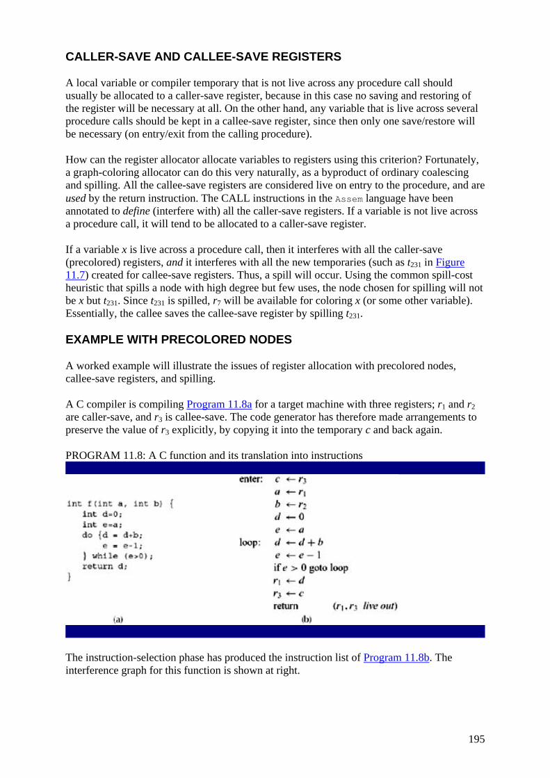
195

CALLER-SAVE AND CALLEE-SAVE REGISTERS

A local variable or compiler temporary that is not live across any procedure call should usually be allocated to a caller-save register, because in this case no saving and restoring of the register will be necessary at all. On the other hand, any variable that is live across several procedure calls should be kept in a callee-save register, since then only one save/restore will be necessary (on entry/exit from the calling procedure).

How can the register allocator allocate variables to registers using this criterion? Fortunately, a graph-coloring allocator can do this very naturally, as a byproduct of ordinary coalescing and spilling. All the callee-save registers are considered live on entry to the procedure, and are used by the return instruction. The CALL instructions in the Assem language have been annotated to define (interfere with) all the caller-save registers. If a variable is not live across a procedure call, it will tend to be allocated to a caller-save register.

If a variable x is live across a procedure call, then it interferes with all the caller-save (precolored) registers, and it interferes with all the new temporaries (such as t231 in Figure 11.7) created for callee-save registers. Thus, a spill will occur. Using the common spill-cost heuristic that spills a node with high degree but few uses, the node chosen for spilling will not be x but t231. Since t231 is spilled, r7 will be available for coloring x (or some other variable). Essentially, the callee saves the callee-save register by spilling t231.

EXAMPLE WITH PRECOLORED NODES

A worked example will illustrate the issues of register allocation with precolored nodes, callee-save registers, and spilling.

A C compiler is compiling Program 11.8a for a target machine with three registers; r1 and r2 are caller-save, and r3 is callee-save. The code generator has therefore made arrangements to preserve the value of r3 explicitly, by copying it into the temporary c and back again.

PROGRAM 11.8: A C function and its translation into instructions

The instruction-selection phase has produced the instruction list of Program 11.8b. The interference graph for this function is shown at right.

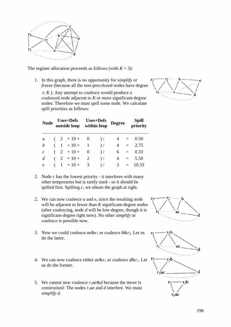
196

The register allocation proceeds as follows (with K = 3):

1. In this graph, there is no opportunity for simplify or freeze (because all the non-precolored nodes have degree ≥ K ). Any attempt to coalesce would produce a coalesced node adjacent to K or more significant-degree nodes. Therefore we must spill some node. We calculate spill priorities as follows:

Node Uses+Defs outside loop

Uses+Defs within loop Degree Spill

priority

a ( 2 + 10 × 0 ) / 4 = 0.50 b ( 1 + 10 × 1 ) / 4 = 2.75 c ( 2 + 10 × 0 ) / 6 = 0.33 d ( 2 + 10 × 2 ) / 4 = 5.50 e ( 1 + 10 × 3 ) / 3 = 10.33

2. Node c has the lowest priority - it interferes with many other temporaries but is rarely used - so it should be spilled first. Spilling c, we obtain the graph at right.

2. We can now coalesce a and e, since the resulting node will be adjacent to fewer than K significant-degree nodes (after coalescing, node d will be low-degree, though it is significant-degree right now). No other simplify or coalesce is possible now.

3. Now we could coalesce ae&r1 or coalesce b&r2. Let us do the latter.

4. We can now coalesce either ae&r1 or coalesce d&r1. Let

us do the former.

5. We cannot now coalesce r1ae&d because the move is

constrained: The nodes r1ae and d interfere. We must simplify d.

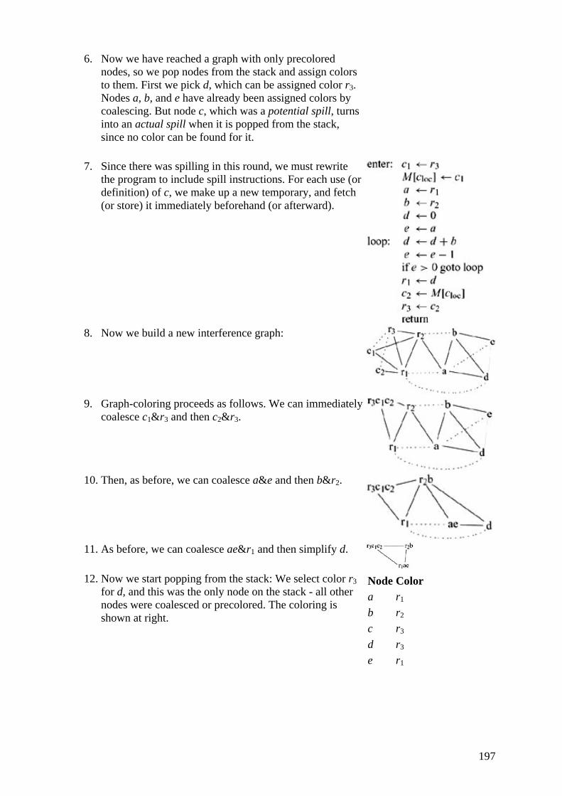
197

6. Now we have reached a graph with only precolored nodes, so we pop nodes from the stack and assign colors to them. First we pick d, which can be assigned color r3. Nodes a, b, and e have already been assigned colors by coalescing. But node c, which was a potential spill, turns into an actual spill when it is popped from the stack, since no color can be found for it.

7. Since there was spilling in this round, we must rewrite the program to include spill instructions. For each use (or definition) of c, we make up a new temporary, and fetch (or store) it immediately beforehand (or afterward).

8. Now we build a new interference graph:

9. Graph-coloring proceeds as follows. We can immediately coalesce c1&r3 and then c2&r3.

10. Then, as before, we can coalesce a&e and then b&r2.

11. As before, we can coalesce ae&r1 and then simplify d.

12. Now we start popping from the stack: We select color r3 for d, and this was the only node on the stack - all other nodes were coalesced or precolored. The coloring is shown at right.

Node Color a r1 b r2 c r3 d r3 e r1

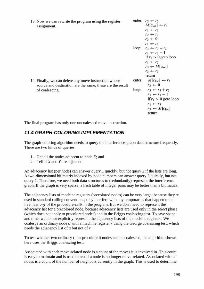
198

13. Now we can rewrite the program using the register assignment.

14. Finally, we can delete any move instruction whose

source and destination are the same; these are the result of coalescing.

The final program has only one uncoalesced move instruction.

11.4 GRAPH-COLORING IMPLEMENTATION

The graph-coloring algorithm needs to query the interference-graph data structure frequently. There are two kinds of queries:

1. Get all the nodes adjacent to node X; and 2. Tell if X and Y are adjacent.

An adjacency list (per node) can answer query 1 quickly, but not query 2 if the lists are long. A two-dimensional bit matrix indexed by node numbers can answer query 2 quickly, but not query 1. Therefore, we need both data structures to (redundantly) represent the interference graph. If the graph is very sparse, a hash table of integer pairs may be better than a bit matrix.

The adjacency lists of machine registers (precolored nodes) can be very large; because they're used in standard calling conventions, they interfere with any temporaries that happen to be live near any of the procedure-calls in the program. But we don't need to represent the adjacency list for a precolored node, because adjacency lists are used only in the select phase (which does not apply to precolored nodes) and in the Briggs coalescing test. To save space and time, we do not explicitly represent the adjacency lists of the machine registers. We coalesce an ordinary node a with a machine register r using the George coalescing test, which needs the adjacency list of a but not of r.

To test whether two ordinary (non-precolored) nodes can be coalesced, the algorithm shown here uses the Briggs coalescing test.

Associated with each move-related node is a count of the moves it is involved in. This count is easy to maintain and is used to test if a node is no longer move-related. Associated with all nodes is a count of the number of neighbors currently in the graph. This is used to determine

199

whether a node is of significant degree during coalescing, and whether a node can be removed from the graph during simplification.

It is important to be able to quickly perform each simplify step (removing a low-degree non-move-related node), each coalesce step, and each freeze step. To do this, we maintain four work lists:

• Low-degree non-move-related nodes (simplifyWorklist); • Move instructions that might be coalesceable (worklistMoves); • Low-degree move-related nodes (freezeWorklist); • High-degree nodes (spillWorklist).

Using these work lists, we avoid quadratic time blowup in finding coalesceable nodes.

DATA STRUCTURES

The algorithm maintains these data structures to keep track of graph nodes and move edges:

Node work lists, sets, and stacks The following lists and sets are always mutually disjoint and every node is always in exactly one of the sets or lists.

• precolored: machine registers, preassigned a color. • initial: temporary registers, not precolored and not yet processed. • simplifyWorklist: list of low-degree non-move-related nodes. • freezeWorklist: low-degree move-related nodes. • spillWorklist: high-degree nodes. • spilledNodes: nodes marked for spilling during this round; initially empty. • coalescedNodes: registers that have been coalesced; when u ← v is coalesced, v is

added to this set and u put back on some work list (or vice versa). • coloredNodes: nodes successfully colored. • selectStack: stack containing temporaries removed from the graph.

Since membership in these sets is often tested, the representation of each node should contain an enumeration value telling which set it is in. Since nodes must frequently be added to and removed from these sets, each set can be represented by a doubly linked list of nodes. Initially (on entry to Main), and on exiting RewriteProgram, only the sets precolored and initial are nonempty.

Move sets There are five sets of move instructions, and every move is in exactly one of these sets (after Build through the end of Main).

• coalescedMoves: moves that have been coalesced. • constrainedMoves: moves whose source and target interfere. • frozenMoves: moves that will no longer be considered for coalescing. • worklistMoves: moves enabled for possible coalescing. • activeMoves: moves not yet ready for coalescing.

Like the node work lists, the move sets should be implemented as doubly linked lists, with each move containing an enumeration value identifying which set it belongs to.

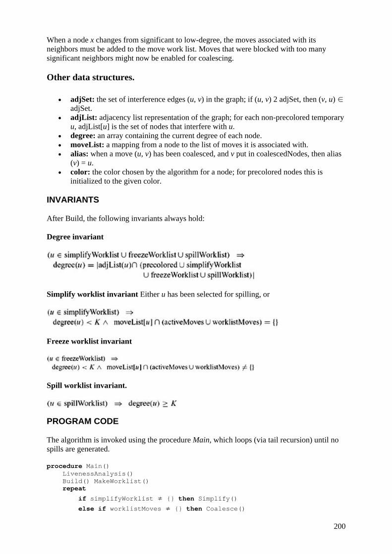
200

When a node x changes from significant to low-degree, the moves associated with its neighbors must be added to the move work list. Moves that were blocked with too many significant neighbors might now be enabled for coalescing.

Other data structures.

• adjSet: the set of interference edges (u, v) in the graph; if (u, v) 2 adjSet, then (v, u) ∈ adjSet.

• adjList: adjacency list representation of the graph; for each non-precolored temporary u, adjList[u] is the set of nodes that interfere with u.

• degree: an array containing the current degree of each node. • moveList: a mapping from a node to the list of moves it is associated with. • alias: when a move (u, v) has been coalesced, and v put in coalescedNodes, then alias

(v) = u. • color: the color chosen by the algorithm for a node; for precolored nodes this is

initialized to the given color.

INVARIANTS

After Build, the following invariants always hold:

Degree invariant

Simplify worklist invariant Either u has been selected for spilling, or

Freeze worklist invariant

Spill worklist invariant.

PROGRAM CODE

The algorithm is invoked using the procedure Main, which loops (via tail recursion) until no spills are generated.

procedure Main() LivenessAnalysis() Build() MakeWorklist() repeat

if simplifyWorklist ≠ {} then Simplify() else if worklistMoves ≠ {} then Coalesce()

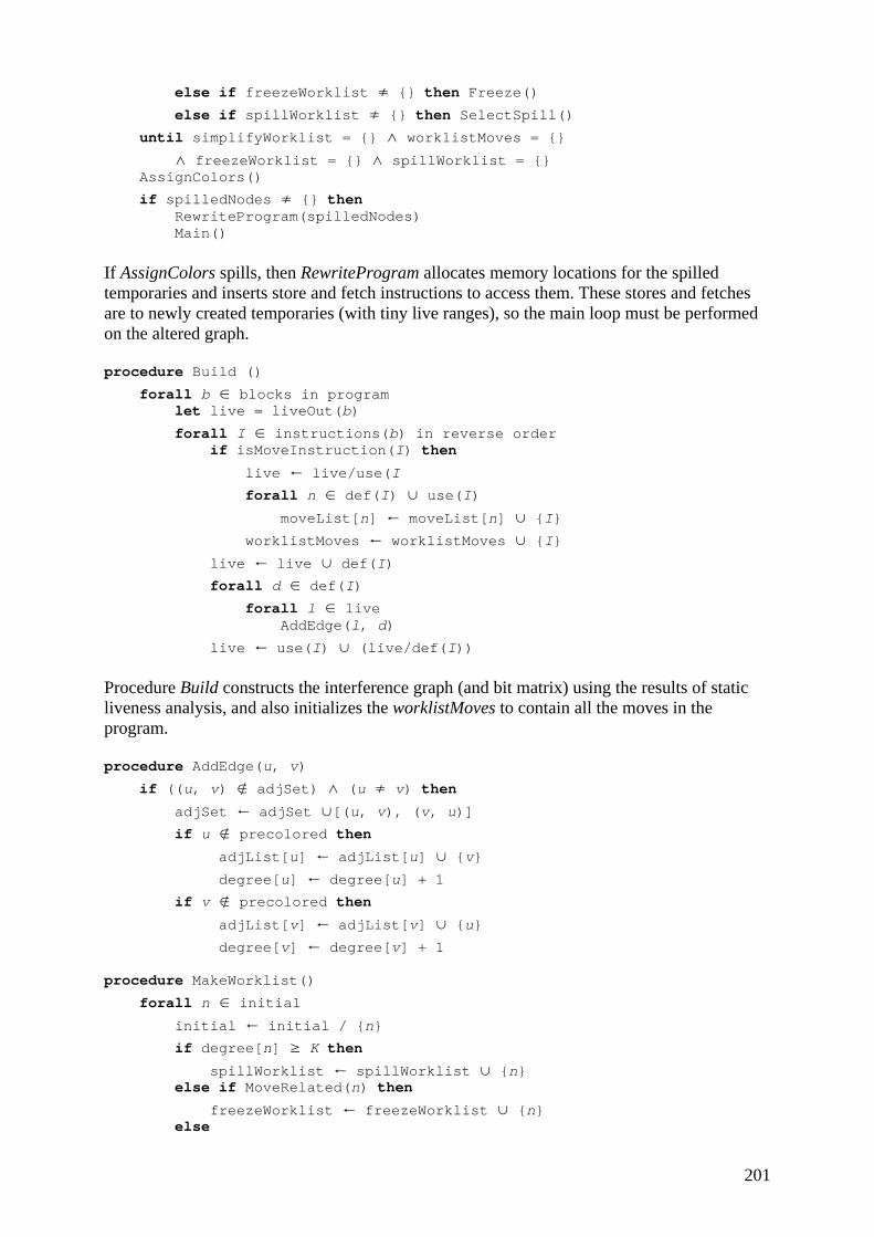
201

else if freezeWorklist ≠ {} then Freeze() else if spillWorklist ≠ {} then SelectSpill() until simplifyWorklist = {} ∧ worklistMoves = {} ∧ freezeWorklist = {} ∧ spillWorklist = {} AssignColors()

if spilledNodes ≠ {} then RewriteProgram(spilledNodes) Main()

If AssignColors spills, then RewriteProgram allocates memory locations for the spilled temporaries and inserts store and fetch instructions to access them. These stores and fetches are to newly created temporaries (with tiny live ranges), so the main loop must be performed on the altered graph.

procedure Build ()

forall b ∈ blocks in program let live = liveOut(b)

forall I ∈ instructions(b) in reverse order if isMoveInstruction(I) then

live ← live/use(I forall n ∈ def(I) ∪ use(I) moveList[n] ← moveList[n] ∪ {I} worklistMoves ← worklistMoves ∪ {I} live ← live ∪ def(I) forall d ∈ def(I) forall l ∈ live AddEdge(l, d)

live ← use(I) ∪ (live/def(I))

Procedure Build constructs the interference graph (and bit matrix) using the results of static liveness analysis, and also initializes the worklistMoves to contain all the moves in the program.

procedure AddEdge(u, v)

if ((u, v) ∉ adjSet) ∧ (u ≠ v) then adjSet ← adjSet ∪[(u, v), (v, u)] if u ∉ precolored then adjList[u] ← adjList[u] ∪ {v} degree[u] ← degree[u] + 1 if v ∉ precolored then adjList[v] ← adjList[v] ∪ {u} degree[v] ← degree[v] + 1 procedure MakeWorklist()

forall n ∈ initial initial ← initial / {n} if degree[n] ≥ K then spillWorklist ← spillWorklist ∪ {n} else if MoveRelated(n) then

freezeWorklist ← freezeWorklist ∪ {n} else

202

simplifyWorklist ← simplifyWorklist ∪ {n} function Adjacent(n)

adjList[n] / (selectStack ∪ coalescedNodes) function NodeMoves (n)

moveList[n] ∩ (activeMoves ∪ worklistMoves) function MoveRelated(n)

NodeMoves(n) ≠ {} procedure Simplify()

let n ∈ simplifyWorklist simplifyWorklist ← simplifyWorklist / {n} push(n, selectStack)

forall m ∈ Adjacent(n) DecrementDegree(m)

Removing a node from the graph involves decrementing the degree of its current neighbors. If the degree of a neighbor is already less than K − 1, then the neighbor must be move-related, and is not added to the simplifyWorklist. When the degree of a neighbor transitions from K to K − 1, moves associated with its neighbors may be enabled.

procedure DecrementDegree(m) let d = degree[m]

degree[m] ← d-1 if d = K then

EnableMoves({m} ∪ Adjacent(m)) spillWorklist ← spillWorklist / {m} if MoveRelated(m) then

freezeWorklist ← freezeWorklist ∪ {m} else

simplifyWorklist ← simplifyWorklist ∪ {m} procedure EnableMoves(nodes)

forall n ∈ nodes forall m ∈ NodeMoves(n) if m ∈ activeMoves then activeMoves ← activeMoves / {m} worklistMoves worklistMoves ∪ {m}

Only moves in the worklistMoves are considered in the coalesce phase. When a move is coalesced, it may no longer be move-related and can be added to the simplify work list by the procedure AddWorkList. OK implements the heuristic used for coalescing a precolored register. Conservative implements the conservative coalescing heuristic.

procedure AddWorkList(u)

if (u ≠ precolored ∧ not(MoveRelated(u)) ∧ degree[u] < K) then freezeWorklist ← freezeWorklist / {u} simplifyWorklist ← simplifyWorklist ∪ {u} function OK(t, r)

degree[t] < K ∩ t ∈ precolored ∩ (t, r) ∈ adjSet

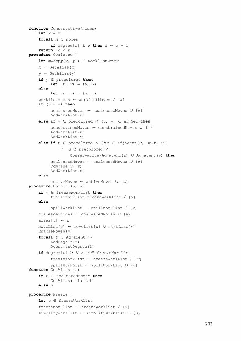
203

function Conservative(nodes) let k = 0

forall n ∈ nodes if degree[n] ≥ K then k ← k + 1 return (k < K) procedure Coalesce()

let m=copy(x, y)) ∈ worklistMoves x ← GetAlias(x) y ← GetAlias(y) if y ∈ precolored then let (u, v) = (y, x) else let (u, v) = (x, y)

worklistMoves ← worklistMoves / {m} if (u = v) then

coalescedMoves ← coalescedMoves ∪ {m} AddWorkList(u)

else if v ∈ precolored ∩ (u, v) ∈ adjSet then constrainedMoves ← constrainedMoves ∪ {m} AddWorkList(u) AddWorkList(v)

else if u ∈ precolored ∧ (∀t ∈ Adjacent(v, OK(t, u/) ∩ u ∉ precolored ∧ Conservative(Adjacent(u) ∪ Adjacent(v) then coalescedMoves ← coalescedMoves ∪ {m} Combine(u, v) AddWorkList(u) else

activeMoves ← activeMoves ∪ {m} procedure Combine(u, v)

if v ∈ freezeWorklist then freezeWorklist freezeWorklist / {v} else

spillWorklist ← spillWorklist / {v} coalescedNodes ← coalescedNodes ∪ {v} alias[v] ← u moveList[u] ← moveList[u] ∪ moveList[v] EnableMoves(v)

forall t ∈ Adjacent(v) AddEdge(t,u) DecrementDegree(t)

if degree[u] ≥ K ∧ u ∈ freezeWorkList freezeWorkList ← freezeWorkList / {u} spillWorkList ← spillWorkList ∪ {u} function GetAlias (n)

if n ∈ coalescedNodes then GetAlias(alias[n]) else n procedure Freeze()

let u ∈ freezeWorklist freezeWorklist ← freezeWorklist / {u} simplifyWorklist ← simplifyWorklist ∪ {u}

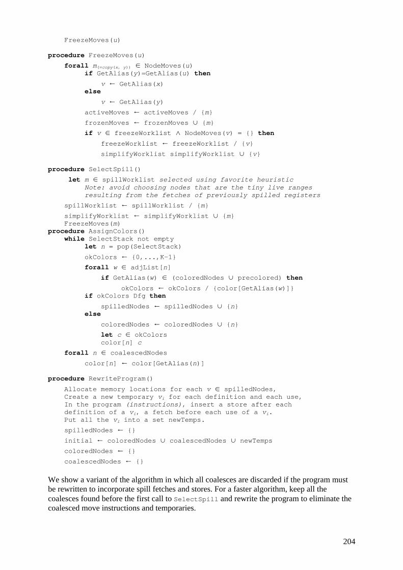
204

FreezeMoves(u) procedure FreezeMoves(u)

forall m(=copy(x, y)) ∈ NodeMoves(u) if GetAlias(y)=GetAlias(u) then

v ← GetAlias(x) else

v ← GetAlias(y) activeMoves ← activeMoves / {m} frozenMoves ← frozenMoves ∪ {m} if v ∈ freezeWorklist ∧ NodeMoves(v) = {} then freezeWorklist ← freezeWorklist / {v} simplifyWorklist simplifyWorklist ∪ {v} procedure SelectSpill()

let m ∈ spillWorklist selected using favorite heuristic Note: avoid choosing nodes that are the tiny live ranges resulting from the fetches of previously spilled registers

spillWorklist ← spillWorklist / {m} simplifyWorklist ← simplifyWorklist ∪ {m} FreezeMoves(m) procedure AssignColors() while SelectStack not empty let n = pop(SelectStack)

okColors ← {0,...,K-1} forall w ∈ adjList[n] if GetAlias(w) ∈ (coloredNodes ∪ precolored) then okColors ← okColors / {color[GetAlias(w)]} if okColors Dfg then

spilledNodes ← spilledNodes ∪ {n} else

coloredNodes ← coloredNodes ∪ {n} let c ∈ okColors color[n] c

forall n ∈ coalescedNodes color[n] ← color[GetAlias(n)] procedure RewriteProgram()

Allocate memory locations for each v ∈ spilledNodes, Create a new temporary vi for each definition and each use, In the program (instructions), insert a store after each definition of a vi, a fetch before each use of a vi. Put all the vi into a set newTemps.

spilledNodes ← {} initial ← coloredNodes ∪ coalescedNodes ∪ newTemps coloredNodes ← {} coalescedNodes ← {}

We show a variant of the algorithm in which all coalesces are discarded if the program must be rewritten to incorporate spill fetches and stores. For a faster algorithm, keep all the coalesces found before the first call to SelectSpill and rewrite the program to eliminate the coalesced move instructions and temporaries.

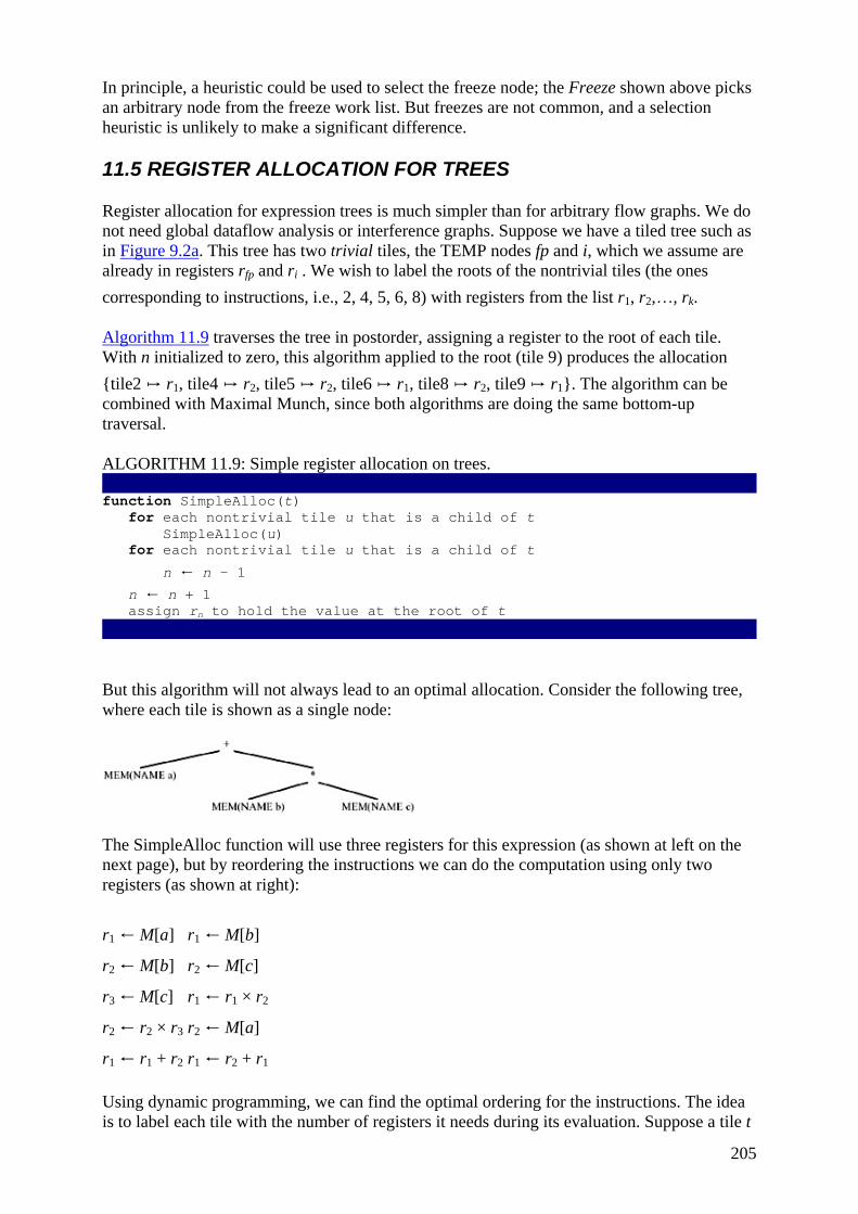
205

In principle, a heuristic could be used to select the freeze node; the Freeze shown above picks an arbitrary node from the freeze work list. But freezes are not common, and a selection heuristic is unlikely to make a significant difference.

11.5 REGISTER ALLOCATION FOR TREES

Register allocation for expression trees is much simpler than for arbitrary flow graphs. We do not need global dataflow analysis or interference graphs. Suppose we have a tiled tree such as in Figure 9.2a. This tree has two trivial tiles, the TEMP nodes fp and i, which we assume are already in registers rfp and ri . We wish to label the roots of the nontrivial tiles (the ones corresponding to instructions, i.e., 2, 4, 5, 6, 8) with registers from the list r1, r2,…, rk.

Algorithm 11.9 traverses the tree in postorder, assigning a register to the root of each tile. With n initialized to zero, this algorithm applied to the root (tile 9) produces the allocation {tile2 ↦ r1, tile4 ↦ r2, tile5 ↦ r2, tile6 ↦ r1, tile8 ↦ r2, tile9 ↦ r1}. The algorithm can be combined with Maximal Munch, since both algorithms are doing the same bottom-up traversal.

ALGORITHM 11.9: Simple register allocation on trees. function SimpleAlloc(t) for each nontrivial tile u that is a child of t SimpleAlloc(u) for each nontrivial tile u that is a child of t

n ← n - 1 n ← n + 1 assign rn to hold the value at the root of t

But this algorithm will not always lead to an optimal allocation. Consider the following tree, where each tile is shown as a single node:

The SimpleAlloc function will use three registers for this expression (as shown at left on the next page), but by reordering the instructions we can do the computation using only two registers (as shown at right):

r1 ← M[a] r1 ← M[b]

r2 ← M[b] r2 ← M[c]

r3 ← M[c] r1 ← r1 × r2

r2 ← r2 × r3 r2 ← M[a]

r1 ← r1 + r2 r1 ← r2 + r1

Using dynamic programming, we can find the optimal ordering for the instructions. The idea is to label each tile with the number of registers it needs during its evaluation. Suppose a tile t

206

has two nontrivial children uleft and uright that require n and m registers, respectively, for their evaluation. If we evaluate uleft first, and hold its result in one register while we evaluate uright, then we have needed max(n, 1 + m) registers for the whole expression rooted at t. Conversely, if we evaluate uright first, then we need max(1 + n, m) registers. Clearly, if n > m, we should evaluate uleft first, and if n < m, we should evaluate uright first. If n = m, we will need n + 1 registers no matter which subexpression is evaluated first.

Algorithm 11.10 labels each tile t with need[t], the number of registers needed to evaluate the subtree rooted at t. It can be generalized to handle tiles with more than two children. Maximal Munch should identify - but not emit - the tiles, simultaneously with the labeling of Algorithm 11.10. The next pass emits Assem instructions for the tiles; wherever a tile has more than one child, the subtrees must be emitted in decreasing order of register need.

ALGORITHM 11.10: Sethi-Ullman labeling algorithm. function Label(t) for each tile u that is a child of t Label(u) if t is trivial

then need[t] ← 0 else if t has two children, uleft and uright then if need[uleft] = need[uright]

then need[t] ← 1 + need[uleft] else need[t] ← max(1, need[uleft], need[uright]) else if t has one child, u

then need[t] ← max(1, need[u] else if t has no children

then need[t] ← 1

Algorithm 11.10 can profitably be used in a compiler that uses graph-coloring register allocation. Emitting the subtrees in decreasing order of need will minimize the number of simultaneously live temporaries and reduce the number of spills.

In a compiler without graph-coloring register allocation, Algorithm 11.10 is used as a pre-pass to Algorithm 11.11, which assigns registers as the trees are emitted and also handles spilling cleanly. This takes care of register allocation for the internal nodes of expression trees; allocating registers for explicit TEMPsofthe Tree language would have to be done in some other way. In general, such a compiler would keep almost all program variables in the stack frame, so there would not be many of these explicit TEMPs to allocate.

ALGORITHM 11.11: Sethi-Ullman register allocation for trees. function SethiUllman(t, n) if t has two children, uleft and uright

if need[uleft] ≥ K and need[uright] ≥ K SethiUllman(uright, 0)

n ← n - 1 spill: emit instruction to store reg[uright] SethiUllman(uleft, 0)

unspill: reg[uright] ← "r1"; emit instruction to fetch reg[uright] else if need[uleft] ≥ need[uright] SethiUllman(uleft, n) SethiUllman(uright, n + 1)

207

else need[uleft] < need[uright] SethiUllman(uright, n) SethiUllman(uleft, n)

reg[t] ← "rn" emit OPER(instruction[t], reg[t], [ reg[uleft], reg[uright]]) else if t has one child, u SethiUllman(u, n)

reg[t] ← "rn" emit OPER(instruction[t], reg[t], [reg[u]]) else if t is nontrivial but has no children

reg[t] ← "rn" emit OPER(instruction[t], reg[t], []) else if t is a trivial node TEMP(ri)

reg[t] ← "ri"

PROGRAM GRAPH COLORING

Implement graph-coloring register allocation as two modules: Color, which does just the graph coloring itself, and RegAlloc, which manages spilling and calls upon Color as a subroutine. To keep things simple, do not implement spilling or coalescing; this simplifies the algorithm considerably.

package RegAlloc; public class RegAlloc implements Temp.TempMap { public Assem.InstrList instrs; public String tempMap(Temp temp); public RegAlloc(Frame.Frame f, Assem.InstrList il); } class Color implements TempMap { public TempList spills(); public String tempMap(Temp t); public Color(InterferenceGraph ig, TempMap initial, TempList registers); }

Given an interference graph, an initial allocation (precoloring) of some temporaries imposed by calling conventions, and a list of colors (registers), color produces an extension of the initial allocation. The resulting allocation assigns all temps used in the flow graph, making use of registers from the registers list.

The initial allocation is the frame (which implements a TempMap describing precolored temporaries); the registers argument is just the list of all machine registers, Frame.registers (see page 251). The registers in the initial allocation can also appear in the registers argument to Color, since it's OK to use them to color other nodes as well.

The result of Color is a TempMap (that is, Color implements TempMap) describing the register allocation, along with a list of spills. The result of RegAlloc - if there were no spills - is an identical TempMap, which can be used in final assembly-code emission as an argument to Assem.format.

A better Color interface would have a spillCost argument that specifies the spilling cost of each temporary. This can be just the number of uses and defs, or better yet, uses and defs

208

weighted by occurrence in loops and nested loops. A naive spillCost that just returns 1 for every temporary will also work.

A simple implementation of the coloring algorithm without coalescing requires only one work list: the simplifyWorklist, which contains all non-precolored, nonsimplified nodes of degree less than K . Obviously, no freezeWorklist is necessary. No spillWorklist is necessary either, if we are willing to look through all the nodes in the original graph for a spill candidate every time the simplifyWorklist becomes empty.

With only a simplifyWorklist, the doubly linked representation is not necessary: This work list can be implemented as a singly linked list or a stack, since it is never accessed "in the middle."

ADVANCED PROJECT: SPILLING

Implement spilling, so that no matter how many parameters and locals a MiniJava program has, you can still compile it.

ADVANCED PROJECT: COALESCING

Implement coalescing, to eliminate practically all the MOVE instructions from the program.

FURTHER READING

Kempe [1879] invented the simplification algorithm that colors graphs by removing vertices of degree < K. Chaitin [1982] formulated register allocation as a graph-coloring problem - using Kempe's algorithm to color the graph - and performed copy propagation by (nonconservatively) coalescing noninterfering move-related nodes before coloring the graph. Briggs et al. [1994] improved the algorithm with the idea of optimistic spilling, and also avoided introducing spills by using the conservative coalescing heuristic before coloring the graph. George and Appel [1996] found that there are more opportunities for coalescing if conservative coalescing is done during simplification instead of beforehand, and developed the work-list algorithm presented in this chapter.

Ershov [1958] developed the algorithm for optimal register allocation on expression trees; Sethi and Ullman [1970] generalized this algorithm and showed how it should handle spills.

EXERCISES

• 11.1 The following program has been compiled for a machine with three registers r1, r2, r3; r1 and r2 are (caller-save) argument registers and r3 is a callee-save register. Construct the interference graph and show the steps of the register allocation process in detail, as on pages 229−232. When you coalesce two nodes, say whether you are using the Briggs or George criterion.

Hint: When two nodes are connected by an interference edge andamove edge, you may delete the move edge; this is called constrain and is accomplished by the first else if clause of procedure Coalesce.

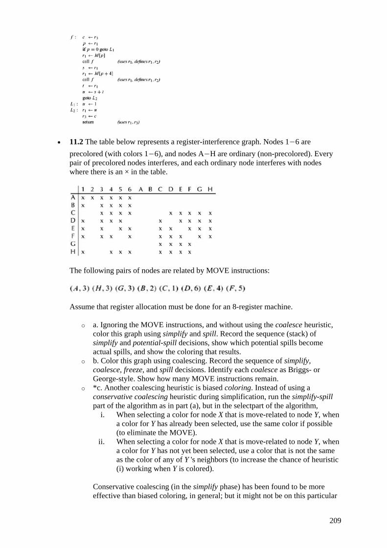
209

• 11.2 The table below represents a register-interference graph. Nodes 1−6 are precolored (with colors 1−6), and nodes A−H are ordinary (non-precolored). Every pair of precolored nodes interferes, and each ordinary node interferes with nodes where there is an × in the table.

The following pairs of nodes are related by MOVE instructions:

Assume that register allocation must be done for an 8-register machine.

o a. Ignoring the MOVE instructions, and without using the coalesce heuristic, color this graph using simplify and spill. Record the sequence (stack) of simplify and potential-spill decisions, show which potential spills become actual spills, and show the coloring that results.

o b. Color this graph using coalescing. Record the sequence of simplify, coalesce, freeze, and spill decisions. Identify each coalesce as Briggs- or George-style. Show how many MOVE instructions remain.

o *c. Another coalescing heuristic is biased coloring. Instead of using a conservative coalescing heuristic during simplification, run the simplify-spill part of the algorithm as in part (a), but in the selectpart of the algorithm,

i. When selecting a color for node X that is move-related to node Y, when a color for Y has already been selected, use the same color if possible (to eliminate the MOVE).

ii. When selecting a color for node X that is move-related to node Y, when a color for Y has not yet been selected, use a color that is not the same as the color of any of Y 's neighbors (to increase the chance of heuristic (i) working when Y is colored).

Conservative coalescing (in the simplify phase) has been found to be more effective than biased coloring, in general; but it might not be on this particular

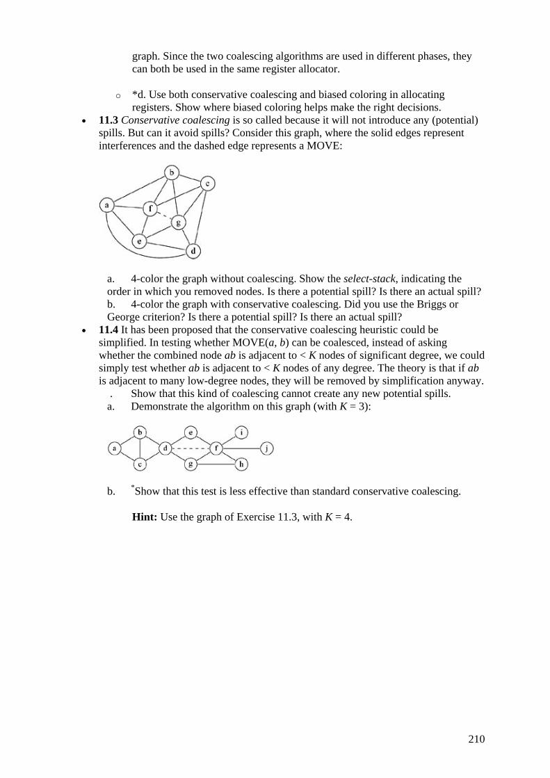
210

graph. Since the two coalescing algorithms are used in different phases, they can both be used in the same register allocator.

o *d. Use both conservative coalescing and biased coloring in allocating registers. Show where biased coloring helps make the right decisions.

• 11.3 Conservative coalescing is so called because it will not introduce any (potential) spills. But can it avoid spills? Consider this graph, where the solid edges represent interferences and the dashed edge represents a MOVE:

a. 4-color the graph without coalescing. Show the select-stack, indicating the order in which you removed nodes. Is there a potential spill? Is there an actual spill? b. 4-color the graph with conservative coalescing. Did you use the Briggs or George criterion? Is there a potential spill? Is there an actual spill?

• 11.4 It has been proposed that the conservative coalescing heuristic could be simplified. In testing whether MOVE(a, b) can be coalesced, instead of asking whether the combined node ab is adjacent to < K nodes of significant degree, we could simply test whether ab is adjacent to < K nodes of any degree. The theory is that if ab is adjacent to many low-degree nodes, they will be removed by simplification anyway.

. Show that this kind of coalescing cannot create any new potential spills. a. Demonstrate the algorithm on this graph (with K = 3):

b. *Show that this test is less effective than standard conservative coalescing.

Hint: Use the graph of Exercise 11.3, with K = 4.

211

Chapter 12: Putting It All Together de-bug: to eliminate errors in or malfunctions of


OVERVIEW

Chapters 2-11 have described the fundamental components of a good compiler: a front end, which does lexical analysis, parsing, construction of abstract syntax, type-checking, and translation to intermediate code; and a back end, which does instruction selection, dataflow analysis, and register allocation.

What lessons have we learned? We hope that the reader has learned about the algorithms used in different components of a compiler and the interfaces used to connect the components. But the authors have also learned quite a bit from the exercise.

Our goal was to describe a good compiler that is, to use Einstein's phrase, "as simple as possible - but no simpler." we will now discuss the thorny issues that arose in designing the MiniJava compiler.

Structured l-values Java (and MiniJava) have no record or array variables, as C, C++, and Pascal do. Instead, all object and array values are really just pointers to heap-allocated data. Implementing structured l-values requires some care but not too many new insights.

Tree intermediate representation The Tree language has a fundamental flaw: It does not describe procedure entry and exit. These are handled by opaque procedures inside the Frame module that generate Tree code. This means that a program translated to Trees using, for example, the Pentium-Frame version of Frame will be different from the same program translated using SparcFrame - the Tree representation is not completely machine-independent.

Also, there is not enough information in the trees themselves to simulate the execution of an entire program, since the view shift (page 128) is partly done implicitly by procedure prologues and epilogues that are not represented as Trees. Consequently, there is not enough information to do whole-program optimization (across function boundaries).

The Tree representation is a low-level intermediate representation, useful for instruction selection and intraprocedural optimization. A high-level intermediate representation would preserve more of the source-program semantics, including the notions of nested functions (if applicable), nonlocal variables, object creation (as distinguished from an opaque external function call), and so on. Such a representation would be more tied to a particular family of source languages than the general-purpose Tree language is.

Register allocation Graph-coloring register allocation is widely used in real compilers, but does it belong in a compiler that is supposed to be "as simple as possible"? After all, it requires the use of global dataflow (liveness) analysis, construction of interference graphs, and so on. This makes the back end of the compiler significantly bigger.

It is instructive to consider what the MiniJava compiler would be like without it. We could keep all local variables in the stack frame, fetching them into temporaries only when they are

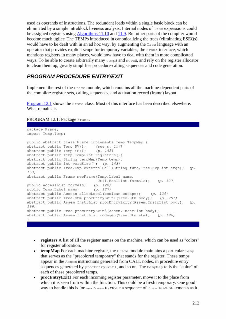
212

used as operands of instructions. The redundant loads within a single basic block can be eliminated by a simple intrablock liveness analysis. Internal nodes of Tree expressions could be assigned registers using Algorithms 11.10 and 11.9. But other parts of the compiler would become much uglier: The TEMPs introduced in canonicalizing the trees (eliminating ESEQs) would have to be dealt with in an ad hoc way, by augmenting the Tree language with an operator that provides explicit scope for temporary variables; the Frame interface, which mentions registers in many places, would now have to deal with them in more complicated ways. To be able to create arbitrarily many temps and moves, and rely on the register allocator to clean them up, greatly simplifies procedure-calling sequences and code generation.

PROGRAM PROCEDURE ENTRY/EXIT

Implement the rest of the Frame module, which contains all the machine-dependent parts of the compiler: register sets, calling sequences, and activation record (frame) layout.

Program 12.1 shows the Frame class. Most of this interface has been described elsewhere. What remains is

PROGRAM 12.1: Package Frame. package Frame; import Temp.Temp; public abstract class Frame implements Temp.TempMap { abstract public Temp RV(); (see p. 157) abstract public Temp FP(); (p. 143) abstract public Temp.TempList registers(); abstract public String tempMap(Temp temp); abstract public int wordSize(); (p. 143) abstract public Tree.Exp externalCall(String func,Tree.ExpList args); (p. 153) abstract public Frame newFrame(Temp.Label name, Util.BoolList formals); (p. 127) public AccessList formals; (p. 128) public Temp.Label name; (p. 127) abstract public Access allocLocal(boolean escape); (p. 129) abstract public Tree.Stm procEntryExit1(Tree.Stm body); (p. 251) abstract public Assem.InstrList procEntryExit2(Assem.InstrList body); (p. 199) abstract public Proc procEntryExit3(Assem.InstrList body); abstract public Assem.InstrList codegen(Tree.Stm stm); (p. 196) }

• registers A list of all the register names on the machine, which can be used as "colors" for register allocation.

• tempMap For each machine register, the Frame module maintains a particular Temp that serves as the "precolored temporary" that stands for the register. These temps appear in the Assem instructions generated from CALL nodes, in procedure entry sequences generated by procEntryExit1, and so on. The tempMap tells the "color" of each of these precolored temps.

• procEntryExit1 For each incoming register parameter, move it to the place from which it is seen from within the function. This could be a fresh temporary. One good way to handle this is for newFrame to create a sequence of Tree.MOVE statements as it

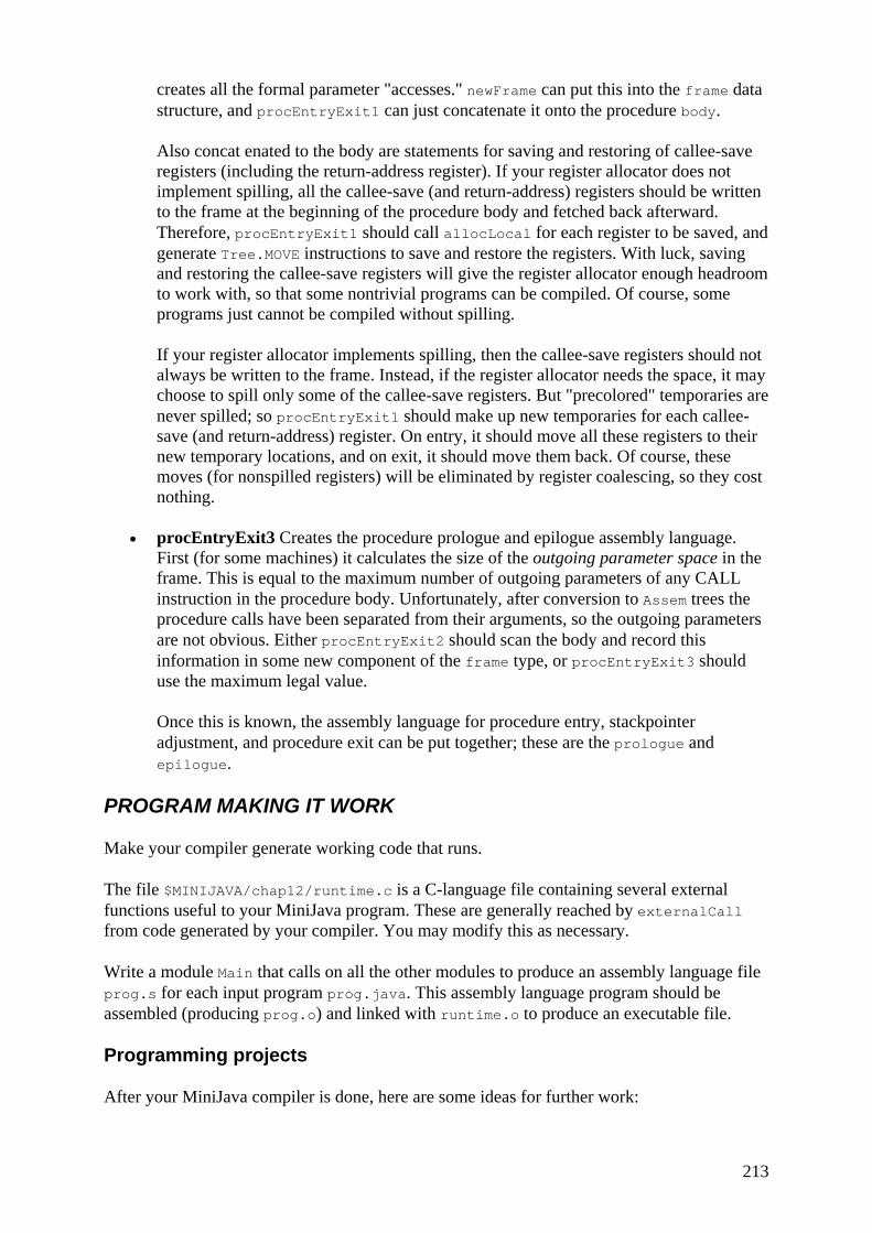
213

creates all the formal parameter "accesses." newFrame can put this into the frame data structure, and procEntryExit1 can just concatenate it onto the procedure body.

Also concat enated to the body are statements for saving and restoring of callee-save registers (including the return-address register). If your register allocator does not implement spilling, all the callee-save (and return-address) registers should be written to the frame at the beginning of the procedure body and fetched back afterward. Therefore, procEntryExit1 should call allocLocal for each register to be saved, and generate Tree.MOVE instructions to save and restore the registers. With luck, saving and restoring the callee-save registers will give the register allocator enough headroom to work with, so that some nontrivial programs can be compiled. Of course, some programs just cannot be compiled without spilling.

If your register allocator implements spilling, then the callee-save registers should not always be written to the frame. Instead, if the register allocator needs the space, it may choose to spill only some of the callee-save registers. But "precolored" temporaries are never spilled; so procEntryExit1 should make up new temporaries for each callee-save (and return-address) register. On entry, it should move all these registers to their new temporary locations, and on exit, it should move them back. Of course, these moves (for nonspilled registers) will be eliminated by register coalescing, so they cost nothing.

• procEntryExit3 Creates the procedure prologue and epilogue assembly language. First (for some machines) it calculates the size of the outgoing parameter space in the frame. This is equal to the maximum number of outgoing parameters of any CALL instruction in the procedure body. Unfortunately, after conversion to Assem trees the procedure calls have been separated from their arguments, so the outgoing parameters are not obvious. Either procEntryExit2 should scan the body and record this information in some new component of the frame type, or procEntryExit3 should use the maximum legal value.

Once this is known, the assembly language for procedure entry, stackpointer adjustment, and procedure exit can be put together; these are the prologue and epilogue.

PROGRAM MAKING IT WORK

Make your compiler generate working code that runs.

The file $MINIJAVA/chap12/runtime.c is a C-language file containing several external functions useful to your MiniJava program. These are generally reached by externalCall from code generated by your compiler. You may modify this as necessary.

Write a module Main that calls on all the other modules to produce an assembly language file prog.s for each input program prog.java. This assembly language program should be assembled (producing prog.o) and linked with runtime.o to produce an executable file.

Programming projects

After your MiniJava compiler is done, here are some ideas for further work:

214

• 12.1 Write a garbage collector (in C) for your MiniJava compiler. You will need to make some modifications to the compiler itself to add descriptors to records and stack frames (see Chapter 13).

• 12.2 Implement inner classes is MiniJava. • 12.3 Implement dataflow analyses such as reaching definitions and available

expressions and use them to implement some of the optimizations discussed in Chapter 17.

• 12.4 Figure out other approaches to improving the assembly language generated by your compiler. Discuss; perhaps implement.

• 12.5 Implement instruction scheduling to fill branch-delay and load-delay slots in the assembly language (for a machine such as the Sparc). Or discuss how such a module could be integrated into the existing compiler; what interfaces would have to change, and in what ways?

• 12.6 Implement "software pipelining" (instruction scheduling around loop iterations) in your compiler (see Chapter 20).

• 12.7 Analyze how adequate the MiniJava language itself would be for writing a compiler. What are the smallest possible additions/changes that would make it a much more useful language?

• 12.8 In the MiniJava language, some object types are recursive and must be implemented as pointers; that is, a value of that type might contain a pointer to another value of the same type (directly or indirectly). But some object types are not recursive, so they could be implemented without pointers. Modify your compiler to take advantage of this by keeping nonrecursive records in the stack frame instead of on the heap.

• 12.9 Similarly, some arrays have bounds that are known at compile time, are not recursive, and are not assigned to other array variables. Modify your compiler so that these arrays are implemented right in the stack frame.

• 12.10 Implement inline expansion of functions (see Section 15.4). • 12.11 Suppose an ordinary MiniJava program were to run on a parallel machine (a

multiprocessor)? How could the compiler automatically make a parallel program out of the original sequential one? Research the approaches.

215

Part Two: Advanced Topics Chapter List Chapter 13: Garbage Collection Chapter 14: Object-Oriented Languages Chapter 15: Functional Programming Languages Chapter 16: Polymorphic Types Chapter 17: Dataflow Analysis Chapter 18: Loop Optimizations Chapter 19: Static Single-Assignment Form Chapter 20: Pipelining and Scheduling Chapter 21: The Memory Hierarchy Appendix A: MiniJava Language Reference Manual

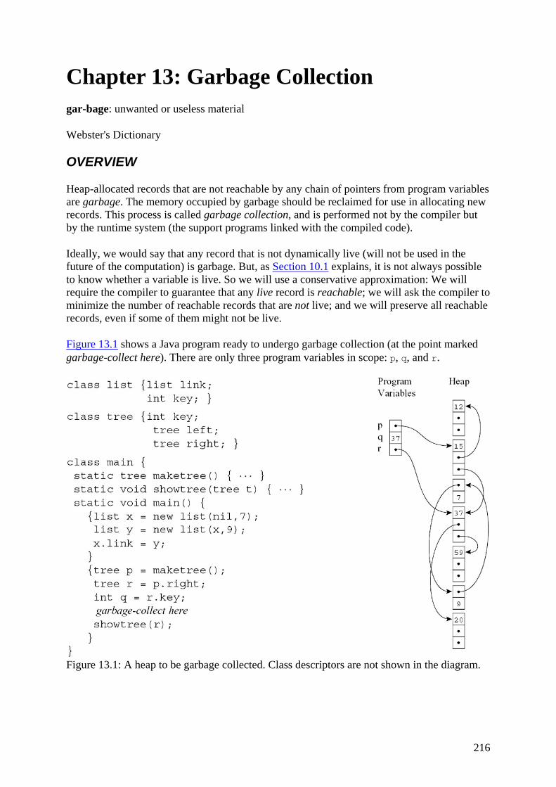
216

Chapter 13: Garbage Collection gar-bage: unwanted or useless material


OVERVIEW

Heap-allocated records that are not reachable by any chain of pointers from program variables are garbage. The memory occupied by garbage should be reclaimed for use in allocating new records. This process is called garbage collection, and is performed not by the compiler but by the runtime system (the support programs linked with the compiled code).

Ideally, we would say that any record that is not dynamically live (will not be used in the future of the computation) is garbage. But, as Section 10.1 explains, it is not always possible to know whether a variable is live. So we will use a conservative approximation: We will require the compiler to guarantee that any live record is reachable; we will ask the compiler to minimize the number of reachable records that are not live; and we will preserve all reachable records, even if some of them might not be live.

Figure 13.1 shows a Java program ready to undergo garbage collection (at the point marked garbage-collect here). There are only three program variables in scope: p, q, and r.

Figure 13.1: A heap to be garbage collected. Class descriptors are not shown in the diagram.

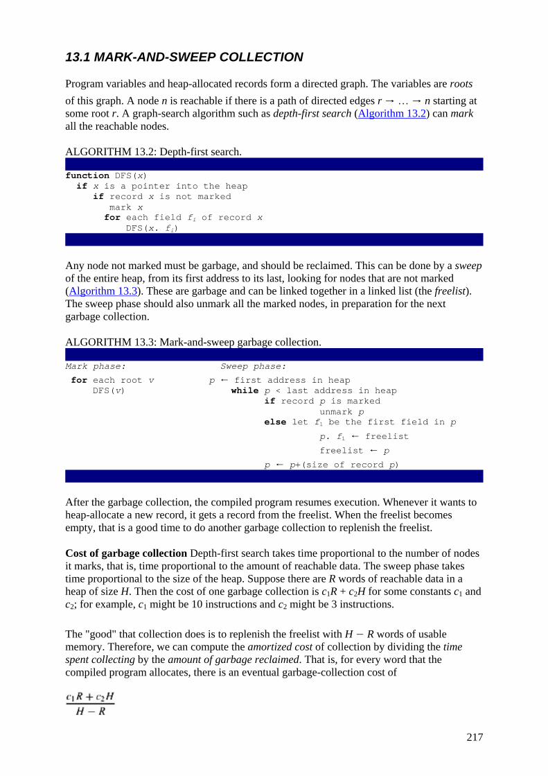
217

13.1 MARK-AND-SWEEP COLLECTION

Program variables and heap-allocated records form a directed graph. The variables are roots of this graph. A node n is reachable if there is a path of directed edges r → … → n starting at some root r. A graph-search algorithm such as depth-first search (Algorithm 13.2) can mark all the reachable nodes.

ALGORITHM 13.2: Depth-first search. function DFS(x) if x is a pointer into the heap if record x is not marked mark x for each field fi of record x DFS(x. fi)

Any node not marked must be garbage, and should be reclaimed. This can be done by a sweep of the entire heap, from its first address to its last, looking for nodes that are not marked (Algorithm 13.3). These are garbage and can be linked together in a linked list (the freelist). The sweep phase should also unmark all the marked nodes, in preparation for the next garbage collection.

ALGORITHM 13.3: Mark-and-sweep garbage collection. Mark phase: Sweep phase:

for each root v p ← first address in heap DFS(v) while p < last address in heap if record p is marked unmark p else let f1 be the first field in p

p. f1 ← freelist freelist ← p p ← p+(size of record p)

After the garbage collection, the compiled program resumes execution. Whenever it wants to heap-allocate a new record, it gets a record from the freelist. When the freelist becomes empty, that is a good time to do another garbage collection to replenish the freelist.

Cost of garbage collection Depth-first search takes time proportional to the number of nodes it marks, that is, time proportional to the amount of reachable data. The sweep phase takes time proportional to the size of the heap. Suppose there are R words of reachable data in a heap of size H. Then the cost of one garbage collection is c1R + c2H for some constants c1 and c2; for example, c1 might be 10 instructions and c2 might be 3 instructions.

The "good" that collection does is to replenish the freelist with H − R words of usable memory. Therefore, we can compute the amortized cost of collection by dividing the time spent collecting by the amount of garbage reclaimed. That is, for every word that the compiled program allocates, there is an eventual garbage-collection cost of

218

If R is close to H, this cost becomes very large: Each garbage collection reclaims only a few words of garbage. If H is much larger than R, then the cost per allocated word is approximately c2, or about 3 instructions of garbage-collection cost per word allocated.

The garbage collector can measure H (the heap size) and H − R (the freelist size) directly. After a collection, if R/H is larger than 0.5 (or some other criterion), the collector should increase H by asking the operating system for more memory. Then the cost per allocated word will be approximately c1 + 2c2, or perhaps 16 instructions per word.

Using an explicit stack The DFS algorithm is recursive, and the maximum depth of its recursion is as long as the longest path in the graph of reachable data. There could be a path of length H in the worst case, meaning that the stack of activation records would be larger than the entire heap!

Figure 13.4: Mark-and-sweep collection.

To attack this problem, we use an explicit stack (instead of recursion), as in Algorithm 13.5. Now the stack could still grow to size H, but at least this is H words and not H activation records. Still, it is unacceptable to require auxiliary stack memory as large as the heap being collected.

ALGORITHM 13.5: Depth-first search using an explicit stack. function DFS(x) if x is a pointer and record x is not marked mark x t 1

stack[t] ← x while t > 0

x ← stack[t]; t ← t - 1 for each field fi of record x

219

if x. fi is a pointer and record x. fi is not marked mark x. fi

t ← t + 1; stack[t] ← x. fi

Pointer reversal After the contents of field x. fi have been pushed on the stack, Algorithm 13.5 will never again look the original location x. fi. This means we can use x. fi to store one element of the stack itself! This all-too-clever idea is called pointer reversal, because x. fi will be made to point back to the record from which x was reached. Then, as the stack is popped, the field x. fi will be restored to its original value.

Algorithm 13.6 requires a field in each record called done, which indicates how many fields in that record have been processed. This takes only a few bits per record (and it can also serve as the mark field).

ALGORITHM 13.6: Depth-first search using pointer reversal. function DFS(x) if x is a pointer and record x is not marked

t ← nil mark x; done[x] 0 while true i done[x] if i < # of fields in record x

y ← x. fi if y is a pointer and record y is not marked

x. fi ← t; t ← x; x ← y mark x; done[x] 0 else

done[x] ← i + 1 else

y ← x; x ← t if x = nil then return

i ← done[x] t ← x. fi; x. fi ← y done[x] ← i + 1

The variable t serves as the top of the stack; every record x on the stack is already marked, and if i = done[x], then x. fi is the "stack link" to the next node down. When popping the stack, x. fi is restored to its original value.

An array of freelists The sweep phase is the same no matter which marking algorithm is used: It just puts the unmarked records on the freelist, and unmarks the marked records. But if records are of many different sizes, a simple linked list will not be very efficient for the allocator. When allocating a record of size n, it may have to search a long way down the list for a free block of that size.

A good solution is to have an array of several freelists, so that freelist[i] is a linked list of all records of size i. The program can allocate a node of size i just by taking the head of freelist[i]; the sweep phase of the collector can put each node of size j at the head of freelist[j].

220

If the program attempts to allocate from an empty freelist[i], it can try to grab a larger record from freelist[j] (for j > i) and split it (putting the unused portion back on freelist[j − i]). If this fails, it is time to call the garbage collector to replenish the freelists.

Fragmentation It can happen that the program wants to allocate a record of size n, and there are many free records smaller than n but none of the right size. This is called external fragmentation. On the other hand, internal fragmentation occurs when the program uses a too-large record without splitting it, so that the unused memory is inside the record instead of outside.

13.2 REFERENCE COUNTS

One day a student came to Moon and said: "I understand how to make a better garbage collector. We must keep a reference count of the pointers to each cons."

Moon patiently told the student the following story:

"One day a student came to Moon and said: ‘I understand how to make a better garbage collector …'"

(MIT-AI koan by Danny Hillis)

Mark-sweep collection identifies the garbage by first finding out what is reachable. Instead, it can be done directly by keeping track of how many pointers point to each record: This is the reference count of the record, and it is stored with each record.

The compiler emits extra instructions so that whenever p is stored into x. fi, the reference count of p is incremented, and the reference count of what x. fi previously pointed to is decremented. If the decremented reference count of some record r reaches zero, then r is put on the freelist and all the other records that r points to have their reference counts decremented.

Instead of decrementing the counts of r. fi when r is put on the freelist, it is better to do this "recursive" decrementing when r is removed from the freelist, for two reasons:

1. It breaks up the "recursive decrementing" work into shorter pieces, so that the program can run more smoothly (this is important only for interactive or real-time programs).

2. The compiler must emit code (at each decrement) to check whether the count has reached zero and put the record on the freelist, but the recursive decrementing will be done only in one place, in the allocator.

Reference counting seems simple and attractive. But there are two major problems:

1. Cycles of garbage cannot be reclaimed. In Figure 13.1, for example, there is a loop of list cells (whose keys are 7 and 9) that are not reachable from program variables; but each has a reference count of 1.

2. Incrementing the reference counts is very expensive indeed. In place of the single machine instruction x. fi ← p, the program must execute

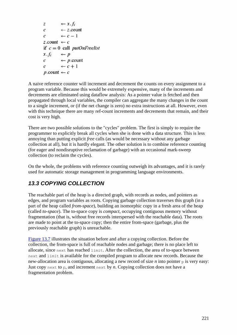
221

A naive reference counter will increment and decrement the counts on every assignment to a program variable. Because this would be extremely expensive, many of the increments and decrements are eliminated using dataflow analysis: As a pointer value is fetched and then propagated through local variables, the compiler can aggregate the many changes in the count to a single increment, or (if the net change is zero) no extra instructions at all. However, even with this technique there are many ref-count increments and decrements that remain, and their cost is very high.

There are two possible solutions to the "cycles" problem. The first is simply to require the programmer to explicitly break all cycles when she is done with a data structure. This is less annoying than putting explicit free calls (as would be necessary without any garbage collection at all), but it is hardly elegant. The other solution is to combine reference counting (for eager and nondisruptive reclamation of garbage) with an occasional mark-sweep collection (to reclaim the cycles).

On the whole, the problems with reference counting outweigh its advantages, and it is rarely used for automatic storage management in programming language environments.

13.3 COPYING COLLECTION

The reachable part of the heap is a directed graph, with records as nodes, and pointers as edges, and program variables as roots. Copying garbage collection traverses this graph (in a part of the heap called from-space), building an isomorphic copy in a fresh area of the heap (called to-space). The to-space copy is compact, occupying contiguous memory without fragmentation (that is, without free records interspersed with the reachable data). The roots are made to point at the to-space copy; then the entire from-space (garbage, plus the previously reachable graph) is unreachable.

Figure 13.7 illustrates the situation before and after a copying collection. Before the collection, the from-space is full of reachable nodes and garbage; there is no place left to allocate, since next has reached limit. After the collection, the area of to-space between next and limit is available for the compiled program to allocate new records. Because the new-allocation area is contiguous, allocating a new record of size n into pointer p is very easy: Just copy next to p, and increment next by n. Copying collection does not have a fragmentation problem.

222

Figure 13.7: Copying collection.

Eventually, the program will allocate enough that next reaches limit; then another garbage collection is needed. The roles of from-space and to-space are swapped, and the reachable data are again copied.

Initiating a collection To start a new collection, the pointer next is initialized to point at the beginning of to-space; as each reachable record in from-space is found, it is copied to to-space at position next, and next incremented by the size of the record.

Forwarding The basic operation of copying collection is forwarding a pointer; that is, given a pointer p that points to from-space, make p point to to-space (Algorithm 13.8).

ALGORITHM 13.8: Forwarding a pointer. function Forward(p) if p points to from-space then if p. f1 points to to-space then return p. f1 else for each field fi of p

next. fi ← p. fi p. f1 ← next next ← next+ size of record p return p. f1 else return p

There are three cases:

1. If p points to a from-space record that has already been copied, then p. f1 is a special forwarding pointer that indicates where the copy is. The forwarding pointer can be identified just by the fact that it points within the to-space, as no ordinary from-space field could point there.

2. If p points to a from-space record that has not yet been copied, then it is copied to location next; and the forwarding pointer is installed into p. f1. It's all right to overwrite the f1 field of the old record, because all the data have already been copied to the to-space at next.

3. If p is not a pointer at all, or if it points outside from-space (to a record outside the garbage-collected arena, or to to-space), then forwarding p does nothing.

223

Cheney's algorithm The simplest algorithm for copying collection uses breadth-first search to traverse the reachable data (Algorithm 13.9, illustrated in Figure 13.10). First, the roots are forwarded. This copies a few records (those reachable directly from root pointers) to to-space, thereby incrementing next.

Figure 13.10: Breadth-first copying collection. ALGORITHM 13.9: Breadth-first copying garbage collection. scan ← next ← beginning of to-space for each root r

r ← Forward(r) while scan < next for each field fi of record at scan scan. fi Forward(scan. fi)

scan ← scan+ size of record at scan

The area between scan and next contains records that have been copied to to-space, but whose fields have not yet been forwarded: In general, these fields point to from-space. The area between the beginning of to-space and scan contains records that have been copied and forwarded, so that all the pointers in this area point to to-space. The while loop (of Algorithm 13.9) moves scan toward next, but copying records will cause next to move also. Eventually, scan catches up with next after all the reachable data are copied to to-space.

Cheney's algorithm requires no external stack, and no pointer reversal: It uses the to-space area between scan and next as the queue of its breadth-first search. This makes it considerably simpler to implement than depth-first search with pointer reversal.

Locality of reference However, pointer data structures copied by breadth-first have poor locality of reference: If a record at address a points to another record at address b, it is likely that a and b will be far apart. Conversely, the record at a + 8 is likely to be unrelated to the

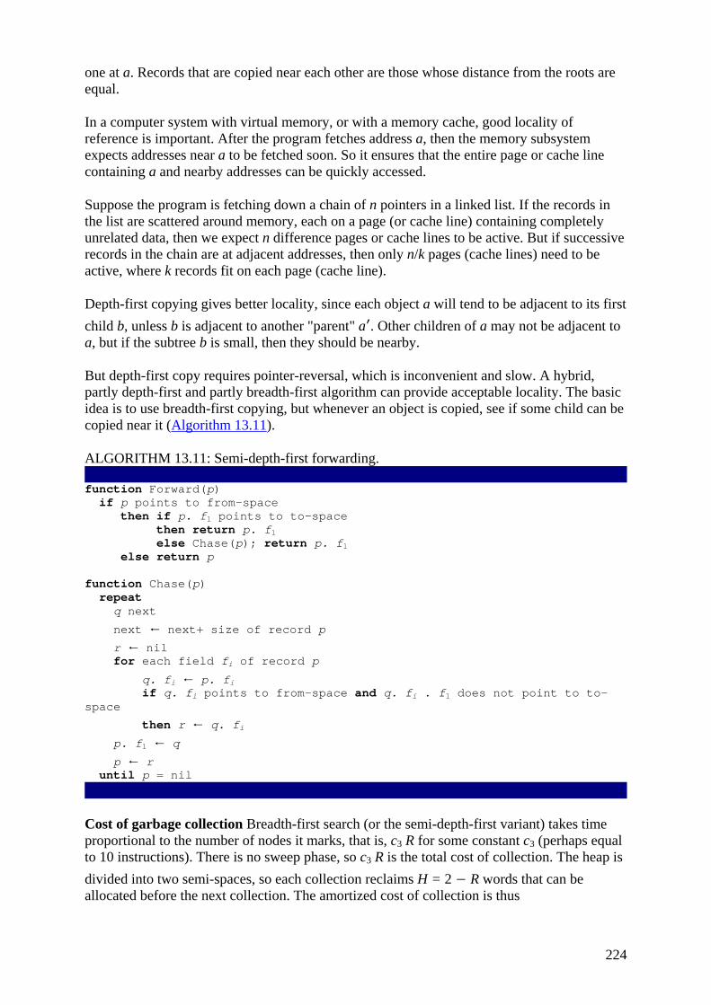
224

one at a. Records that are copied near each other are those whose distance from the roots are equal.

In a computer system with virtual memory, or with a memory cache, good locality of reference is important. After the program fetches address a, then the memory subsystem expects addresses near a to be fetched soon. So it ensures that the entire page or cache line containing a and nearby addresses can be quickly accessed.

Suppose the program is fetching down a chain of n pointers in a linked list. If the records in the list are scattered around memory, each on a page (or cache line) containing completely unrelated data, then we expect n difference pages or cache lines to be active. But if successive records in the chain are at adjacent addresses, then only n/k pages (cache lines) need to be active, where k records fit on each page (cache line).

Depth-first copying gives better locality, since each object a will tend to be adjacent to its first child b, unless b is adjacent to another "parent" a′. Other children of a may not be adjacent to a, but if the subtree b is small, then they should be nearby.

But depth-first copy requires pointer-reversal, which is inconvenient and slow. A hybrid, partly depth-first and partly breadth-first algorithm can provide acceptable locality. The basic idea is to use breadth-first copying, but whenever an object is copied, see if some child can be copied near it (Algorithm 13.11).

ALGORITHM 13.11: Semi-depth-first forwarding. function Forward(p) if p points to from-space then if p. f1 points to to-space then return p. f1 else Chase(p); return p. f1 else return p function Chase(p) repeat q next

next ← next+ size of record p r ← nil for each field fi of record p

q. fi ← p. fi if q. fi points to from-space and q. fi . f1 does not point to to-space

then r ← q. fi p. f1 ← q p ← r until p = nil

Cost of garbage collection Breadth-first search (or the semi-depth-first variant) takes time proportional to the number of nodes it marks, that is, c3 R for some constant c3 (perhaps equal to 10 instructions). There is no sweep phase, so c3 R is the total cost of collection. The heap is divided into two semi-spaces, so each collection reclaims H = 2 − R words that can be allocated before the next collection. The amortized cost of collection is thus

225

instructions per word allocated.

As H grows much larger than R, this cost approaches zero. That is, there is no inherent lower bound to the cost of garbage collection. In a more realistic setting, where H = 4R, the cost would be about 10 instructions per word allocated. This is rather costly in space and time: It requires four times as much memory as reachable data, and requires 40 instructions of overhead for every 4-word object allocated. To reduce both space and time costs significantly, we use generational collection.

13.4 GENERATIONAL COLLECTION

In many programs, newly created objects are likely to die soon; but an object that is still reachable after many collections will probably survive for many collections more. Therefore the collector should concentrate its effort on the "young" data, where there is a higher proportion of garbage.

We divide the heap into generations, with the youngest objects in generation G0; every object in generation G1 is older than any object in G0; everything in G2 is older than anything in G1, and so on.

To collect (by mark-and-sweep or by copying) just G0, just start from the roots and do either depth-first marking or breadth-first copying (or semidepth-first copying). But now the roots are not just program variables: They include any pointer within G1, G2,… that points into G0. If there are too many of these, then processing the roots will take longer than the traversal of reachable objects within G0!

Fortunately, it is rare for an older object to point to a much younger object. In many common programming styles, when an object a is created its fields are immediately initialized; for example, they might be made to point to b and c. But b and c already exist; they are older than a. So we have a newer object pointing to an older object. The only way that an older object b could point to a newer object a is if some field of b is updated long after b is created; this turns out to be rare.

To avoid searching all of G1, G2,… for roots of G0, we make the compiled program remember where there are pointers from old objects to new ones. There are several ways of remembering:

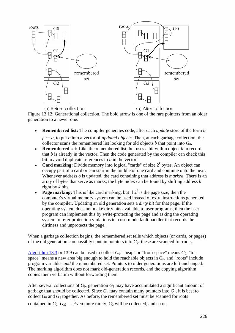
226

Figure 13.12: Generational collection. The bold arrow is one of the rare pointers from an older generation to a newer one.

• Remembered list: The compiler generates code, after each update store of the form b. fi ← a, to put b into a vector of updated objects. Then, at each garbage collection, the collector scans the remembered list looking for old objects b that point into G0.

• Remembered set: Like the remembered list, but uses a bit within object b to record that b is already in the vector. Then the code generated by the compiler can check this bit to avoid duplicate references to b in the vector.

• Card marking: Divide memory into logical "cards" of size 2k bytes. An object can occupy part of a card or can start in the middle of one card and continue onto the next. Whenever address b is updated, the card containing that address is marked. There is an array of bytes that serve as marks; the byte index can be found by shifting address b right by k bits.

• Page marking: This is like card marking, but if 2k is the page size, then the computer's virtual memory system can be used instead of extra instructions generated by the compiler. Updating an old generation sets a dirty bit for that page. If the operating system does not make dirty bits available to user programs, then the user program can implement this by write-protecting the page and asking the operating system to refer protection violations to a usermode fault handler that records the dirtiness and unprotects the page.

When a garbage collection begins, the remembered set tells which objects (or cards, or pages) of the old generation can possibly contain pointers into G0; these are scanned for roots.

Algorithm 13.3 or 13.9 can be used to collect G0: "heap" or "from-space" means G0, "to-space" means a new area big enough to hold the reachable objects in G0, and "roots" include program variables and the remembered set. Pointers to older generations are left unchanged: The marking algorithm does not mark old-generation records, and the copying algorithm copies them verbatim without forwarding them.

After several collections of G0, generation G1 may have accumulated a significant amount of garbage that should be collected. Since G0 may contain many pointers into G1, it is best to collect G0 and G1 together. As before, the remembered set must be scanned for roots contained in G2, G3;…. Even more rarely, G2 will be collected, and so on.

227

Each older generation should be exponentially bigger than the previous one. If G0 is half a megabyte, then G1 should be two megabytes, G2 should be eight megabytes, and so on. An object should be promoted from Gi to Gi+1 when it survives two or three collections of Gi.

Cost of generational collection Without detailed empirical information about the distribution of object lifetimes, we cannot analyze the behavior of generational collection. In practice, however, it is common for the youngest generation to be less than 10% live data. With a copying collector, this means that H / R is 10 in this generation, so that the amortized cost per word reclaimed is c3 R / (10R − R), or about 1 instruction. If the amount of reachable data in G0 is about 50 to 100 kilobytes, then the amount of space "wasted" by having H = 10R in the youngest generation is about a megabyte. In a 50-megabyte multigeneration system, this is a small space cost.

Collecting the older generations can be more expensive. To avoid using too much space, a smaller H / R ratio can be used for older generations. This increases the time cost of an older-generation collection, but these are sufficiently rare that the overall amortized time cost is still good.

Maintaining the remembered set also takes time, approximately 10 instructions per pointer update to enter an object into the remembered set and then process that entry in the remembered set. If the program does many more updates than fresh allocations, then generational collection may be more expensive than nongenerational collection.

13.5 INCREMENTAL COLLECTION

Even if the overall garbage collection time is only a few percent of the computation time, the collector will occasionally interrupt the program for long periods. For interactive or real-time programs this is undesirable. Incremental or concurrent algorithms interleave garbage collection work with program execution to avoid long interruptions.

Terminology The collector tries to collect the garbage; meanwhile, the compiled program keeps changing (mutating) the graph of reachable data, so it is called the mutator. An incremental algorithm is one in which the collector operates only when the mutator requests it; in a concurrent algorithm the collector can operate between or during any instructions executed by the mutator.

Tricolor marking In a mark-sweep or copying garbage collection, there are three classes of records:

• White objects are not yet visited by the depth-first or breadth-first search. • Grey objects have been visited (marked or copied), but their children have not yet

been examined. In mark-sweep collection, these objects are on the stack; in Cheney's copying collection, they are between scan and next.

• Black objects have been marked, and their children also marked. In mark-sweep collection, they have already been popped off the stack; in Cheney's algorithm, they have already been scanned.

The collection starts with all objects white; the collector executes Algorithm 13.13, blackening grey objects and greying their white children. Implicit in changing an object from grey to black is removing it from the stack or queue; implicit in greying an object is putting it into the stack or queue. When there are no grey objects, then all white objects must be garbage.

228

ALGORITHM 13.13: Basic tricolor marking while there are any grey objects select a grey record p for each field fi of p if record p. fi is white color record p. fi grey color record p black

Algorithm 13.13 generalizes all of the mark-sweep and copying algorithms shown so far: Algorithms 13.2, 13.3, 13.5, 13.6, and 13.9. All these algorithms preserve two natural invariants:

1. No black object points to a white object. 2. Every grey object is on the collector's (stack or queue) data structure (which we will

call the grey-set).

While the collector operates, the mutator creates new objects (of what color?) and updates pointer fields of existing objects. If the mutator breaks one of the invariants, then the collection algorithm will not work.

Most incremental and concurrent collection algorithms are based on techniques to allow the mutator to get work done while preserving the invariants. For example:

• Dijkstra, Lamport, et al. Whenever the mutator stores a white pointer a into a black object b, it colors a grey. (The compiler generates extra instructions at each store to check for this.)

• Steele. Whenever the mutator stores a white pointer a into a black object b, it colors b grey (using extra instructions generated by the compiler).

• Boehm, Demers, Shenker. All-black pages are marked read-only in the virtual memory system. Whenever the mutator stores any value into an all-black page, a page fault marks all objects on that page grey (and makes the page writable).

• Baker. Whenever the mutator fetches a pointer b to a white object, it colors b grey. The mutator never possesses a pointer to a white object, so it cannot violate invariant 1. The instructions to check the color of b are generated by the compiler after every fetch.

• Appel, Ellis, Li. Whenever the mutator fetches a pointer b from any virtual-memory page containing any nonblack object, a page-fault handler colors every object on the page black (making children of these objects grey). Thus the mutator never possesses a pointer to a white object.

The first three of these are write-barrier algorithms, meaning that each write (store) by the mutator must be checked to make sure an invariant is preserved. The last two are read-barrier algorithms, meaning that read (fetch) instructions are the ones that must be checked. We have seen write barriers before, for generational collection: Remembered lists, remembered sets, card marking, and page marking are all different implementations of the write barrier. Similarly, the read barrier can be implemented in software (as in Baker's algorithm) or using the virtual-memory hardware.

Any implementation of a write or read barrier must synchronize with the collector. For example, a Dijkstra-style collector might try to change a white node to grey (and put it into the grey-set) at the same time the mutator is also greying the node (and putting it into the

229

grey-set). Thus, software implementations of the read or write barrier will need to use explicit synchronization instructions, which can be expensive.

But implementations using virtual-memory hardware can take advantage of the synchronization implicit in a page fault: If the mutator faults on a page, the operating system will ensure that no other process has access to that page before processing the fault.

13.6 BAKER'S ALGORITHM

Baker's algorithm illustrates the details of incremental collection. It is based on Cheney's copying collection algorithm, so it forwards reachable objects from from-space to to-space. Baker's algorithm is compatible with generational collection, so that the from-space and to-space might be for generation G0, or might be G0 +…+ Gk.

To initiate a garbage collection (which happens when an allocate request fails for lack of unused memory), the roles of the (previous) from-space and to-space are swapped, and all the roots are forwarded; this is called the flip. Then the mutator is resumed; but each time the mutator calls the allocator to get a new record, a few pointers at scan are scanned, so that scan advances toward next. Then a new record is allocated at the end of the to-space by decrementing limit by the appropriate amount.

The invariant is that the mutator has pointers only to to-space (never to from-space). Thus, when the mutator allocates and initializes a new record, that record need not be scanned; when the mutator stores a pointer into an old record, it is only storing a to-space pointer.

If the mutator fetches a field of a record, it might break the invariant. So each fetch is followed by two or three instructions that check whether the fetched pointer points to from-space. If so, that pointer must be forwarded immediately, using the standard forward algorithm.

For every word allocated, the allocator must advance scan by at least one word. When scan=next, the collection terminates until the next time the allocator runs out of space. If the heap is divided into two semi-spaces of size H / 2, and R < H / 4, then scan will catch up with next before next reaches halfway through the to-space; also by this time, no more than half the to-space will be occupied by newly allocated records.

Baker's algorithm copies no more data than is live at the flip. Records allocated during collection are not scanned, so they do not add to the cost of collection. The collection cost is thus c3 R. But there is also a cost to check (at every allocation) whether incremental scanning is necessary; this is proportional to H / 2 − R.

But the largest cost of Baker's algorithm is the extra instructions after every fetch, required to maintain the invariant. If one in every 10 instructions fetches from a heap record, and each of these fetches requires two extra instructions to test whether it is a from-space pointer, then there is at least a 20% overhead cost just to maintain the invariant. All of the incremental or concurrent algorithms that use a software write or read barrier will have a significant cost in overhead of ordinary mutator operations.

230

13.7 INTERFACE TO THE COMPILER

The compiler for a garbage-collected language interacts with the garbage collector by generating code that allocates records, by describing locations of roots for each garbage-collection cycle, and by describing the layout of data records on the heap. For some versions of incremental collection, the compiler must also generate instructions to implement a read or write barrier.

FAST ALLOCATION

Some programming languages, and some programs, allocate heap data (and generate garbage) very rapidly. This is especially true of programs in functional languages, where updating old data is discouraged.

The most allocation (and garbage) one could imagine a reasonable program generating is one word of allocation per store instruction; this is because each word of a heap-allocated record is usually initialized. Empirical measurements show that about one in every seven instructions executed is a store, almost regardless of programming language or program. Thus, we have (at most) 1/7 word of allocation per instruction executed.

Supposing that the cost of garbage collection can be made small by proper tuning of a generational collector, there may still be a considerable cost to create the heap records. To minimize this cost, copying collection should be used so that the allocation space is a contiguous free region; the next free location is next and the end of the region is limit. To allocate one record of size N, the steps are

1. Call the allocate function. 2. Test next + N < limit ? (If the test fails, call the garbage collector.) 3. Move next into result 4. Clear M[next], M[next + 1],…, M[next + N − 1] 5. next ← next + N 6. Return from the allocate function.

A. Move result into some computationally useful place. B. Store useful values into the record.

Steps 1 and 6 should be eliminated by inline expanding the allocate function at each place where a record is allocated. Step 3 can often be eliminated by combining it with step A, and step 4 can be eliminated in favor of step B (steps A and B are not numbered because they are part of the useful computation; they are not allocation overhead).

Steps 2 and 5 cannot be eliminated, but if there is more than one allocation in the same basic block (or in the same trace; see Section 8.2), the comparison and increment can be shared among multiple allocations. By keeping next and limit in registers, steps 2 and 5 can be done in a total of three instructions.

By this combination of techniques, the cost of allocating a record - and then eventually garbage collecting it - can be brought down to about four instructions. This means that programming techniques such as the persistent binary search tree (page 108) can be efficient enough for everyday use.

231

DESCRIBING DATA LAYOUTS

The collector must be able to operate on records of all types: list, tree, or whatever the program has declared. It must be able to determine the number of fields in each record, and whether each field is a pointer.

For statically typed languages such as Pascal, or for object-oriented languages such as Java or Modula-3, the simplest way to identify heap objects is to have the first word of every object point to a special type- or class-descriptor record. This record tells the total size of the object and the location of each pointer field.

For statically typed languages this is an overhead of one word per record to serve the garbage collector. But object-oriented languages need this descriptor pointer in every object just to implement dynamic method lookup, so that there is no additional per-object overhead attributable to garbage collection.

The type- or class-descriptor must be generated by the compiler from the static type information calculated by the semantic analysis phase of the compiler. The descriptor pointer will be the argument to the runtime system's alloc function.

In addition to describing every heap record, the compiler must identify to the collector every pointer-containing temporary and local variable, whether it is in a register or in an activation record. Because the set of live temporaries can change at every instruction, the pointer map is different at every point in the program. Therefore, it is simpler to describe the pointer map only at points where a new garbage collection can begin. These are at calls to the alloc function; and also, since any function call might be calling a function which in turn calls alloc, the pointer map must be described at each function call.

The pointer map is best keyed by return addresses: A function call at location a is best described by its return address immediately after a, because the return address is what the collector will see in the very next activation record. The data structure maps return addresses to live-pointer sets; for each pointer that is live immediately after the call, the pointer map tells its register or frame location.

To find all the roots, the collector starts at the top of the stack and scans downward, frame by frame. Each return address keys the pointer-map entry that describes the next frame. In each frame, the collector marks (or forwards, if copying collection) from the pointers in that frame.

Callee-save registers need special handling. Suppose function f calls g, which calls h. Function h knows that it saved some of the callee-save registers in its frame and mentions this fact in its pointer map; but h does not know which of these registers are pointers. Therefore the pointer map for g must describe which of its callee-save registers contain pointers at the call to h and which are "inherited" from f.

DERIVED POINTERS

Sometimes a compiled program has a pointer that points into the middle of a heap record, or that points before or after the record. For example, the expression a[i-2000] can be calculated internally as M[a-2000+i]:

232

If the expression a[i-2000] occurs inside a loop, the compiler might choose to hoist t1 ← a − 2000 outside the loop to avoid recalculating it in each iteration. If the loop also contains an alloc, and a garbage collection occurs while t1 is live, will the collector be confused by a pointer t1 that does not point to the beginning of an object, or (worse yet) that points to an unrelated object?

We say that the t1 is derived from the base pointer a. The pointer map must identify each derived pointer and tell the base pointer from which it is derived. Then, when the collector relocates a to address a′, it must adjust t1 to point to address t1 + a′ − a.

Of course, this means that a must remain live as long as t1 is live. Consider the loop at left, implemented as shown at right:

let r1 ← 100 var a := intarray[100] of 0 r2 ← 0 call alloc

a ← r1 in t1 ← a - 2000 for i := 1930 to 1990 i ← 1930 do f(a[i-2000]) L1 : r1 ← M[t1 + i] call f

end L2 : if i ≤ 1990 goto L1

If there are no other uses of a, then the temporary a appears dead after the assignment to t1. But then the pointer map associated with the return address L2 would not be able to "explain" t1 adequately. Therefore, for purposes of the compiler's liveness analysis, a derived pointer implicitly keeps its base pointer live.

PROGRAM DESCRIPTORS

Implement record descriptors and pointer maps for the MiniJava compiler.

For each record-type declaration, make a string literal to serve as the record descriptor. The length of the string should be equal to the number of fields in the record. The ith byte of the string should be p if the ith field of the record is a pointer (string, record, or array), or n if the ith field is a nonpointer.

The allocRecord function should now take the record descriptor string (pointer) instead of a length; the allocator can obtain the length from the string literal. Then allocRecord should store this descriptor pointer at field zero of the record. Modify the runtime system appropriately.

The user-visible fields of the record will now be at offsets 1, 2, 3,… instead of 0, 1, 2,…; adjust the compiler appropriately.

Design a descriptor format for arrays, and implement it in the compiler and runtime system.

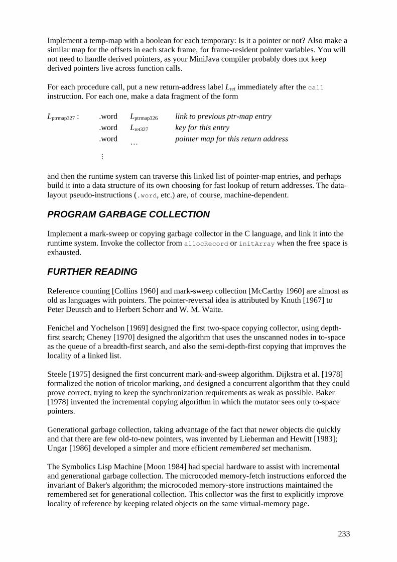
233

Implement a temp-map with a boolean for each temporary: Is it a pointer or not? Also make a similar map for the offsets in each stack frame, for frame-resident pointer variables. You will not need to handle derived pointers, as your MiniJava compiler probably does not keep derived pointers live across function calls.

For each procedure call, put a new return-address label Lret immediately after the call instruction. For each one, make a data fragment of the form

Lptrmap327 : .word Lptrmap326 link to previous ptr-map entry .word Lret327 key for this entry .word … pointer map for this return address

⋮

and then the runtime system can traverse this linked list of pointer-map entries, and perhaps build it into a data structure of its own choosing for fast lookup of return addresses. The data-layout pseudo-instructions (.word, etc.) are, of course, machine-dependent.

PROGRAM GARBAGE COLLECTION

Implement a mark-sweep or copying garbage collector in the C language, and link it into the runtime system. Invoke the collector from allocRecord or initArray when the free space is exhausted.

FURTHER READING

Reference counting [Collins 1960] and mark-sweep collection [McCarthy 1960] are almost as old as languages with pointers. The pointer-reversal idea is attributed by Knuth [1967] to Peter Deutsch and to Herbert Schorr and W. M. Waite.

Fenichel and Yochelson [1969] designed the first two-space copying collector, using depth-first search; Cheney [1970] designed the algorithm that uses the unscanned nodes in to-space as the queue of a breadth-first search, and also the semi-depth-first copying that improves the locality of a linked list.

Steele [1975] designed the first concurrent mark-and-sweep algorithm. Dijkstra et al. [1978] formalized the notion of tricolor marking, and designed a concurrent algorithm that they could prove correct, trying to keep the synchronization requirements as weak as possible. Baker [1978] invented the incremental copying algorithm in which the mutator sees only to-space pointers.

Generational garbage collection, taking advantage of the fact that newer objects die quickly and that there are few old-to-new pointers, was invented by Lieberman and Hewitt [1983]; Ungar [1986] developed a simpler and more efficient remembered set mechanism.

The Symbolics Lisp Machine [Moon 1984] had special hardware to assist with incremental and generational garbage collection. The microcoded memory-fetch instructions enforced the invariant of Baker's algorithm; the microcoded memory-store instructions maintained the remembered set for generational collection. This collector was the first to explicitly improve locality of reference by keeping related objects on the same virtual-memory page.

234

As modern computers rarely use microcode, and a modern general-purpose processor embedded in a general-purpose memory hierarchy tends to be an order of magnitude faster and cheaper than a computer with special-purpose instructions and memory tags, attention turned in the late 1980s to algorithms that could be implemented with standard RISC instructions and standard virtual-memory hardware. Appel et al. [1988] use virtual memory to implement a read barrier in a truly concurrent variant of Baker's algorithm. Shaw [1988] uses virtual-memory dirty bits to implement a write barrier for generational collection, and Boehm et al. [1991] make the same simple write barrier serve for concurrent generational mark-and-sweep. Write barriers are cheaper to implement than read barriers, because stores to old pages are rarer than fetches from to-space, and a write barrier merely needs to set a dirty bit and continue with minimal interruption of the mutator. Sobalvarro [1988] invented the card marking technique, which uses ordinary RISC instructions without requiring interaction with the virtual-memory system.

Appel and Shao [1996] describe techniques for fast allocation of heap records and discuss several other efficiency issues related to garbage-collected systems.

Branquart and Lewi [1971] describe pointer maps communicated from a compiler to its garbage collector; Diwan et al. [1992] tie pointer maps to return addresses, show how to handle derived pointers, and compress the maps to save space.

Appel [1992, Chapter 12] shows that compilers for functional languages must be careful about closure representations; using simple static links (for example) can keep enormous amounts of data reachable, preventing the collector from reclaiming it.

Boehm and Weiser [1988] describe conservative collection, where the compiler does not inform the collector which variables and record fields contain pointers, so the collector must "guess." Any bit pattern pointing into the allocated heap is assumed to be a possible pointer and keeps the pointed-to record live. However, since the bit pattern might really be meant as an integer, the object cannot be moved (which would change the possible integer), and some garbage objects may not be reclaimed. Wentworth [1990] points out that such an integer may (coincidentally) point to the root of a huge garbage data structure, which therefore will not be reclaimed; so conservative collection will occasionally suffer from a disastrous space leak. Boehm [1993] describes several techniques for making these disasters unlikely: For example, if the collector ever finds an integer pointing to address X that is not a currently allocated object, it should blacklist that address so that the allocator will never allocate an object there. Boehm [1996] points out that even a conservative collector needs some amount of compiler assistance: If a derived pointer can point outside the bounds of an object, then its base pointer must be kept live as long as the derived pointer exists.

Page 481 discusses some of the literature on improving the cache performance of garbage-collected systems.

Cohen [1981] comprehensively surveys the first two decades of garbagecollection research; Wilson [1997] describes and discusses more recent work. Jones and Lins [1996] offer a comprehensive textbook on garbage collection.

EXERCISES

• *13.1 Analyze the cost of mark-sweep versus copying collection. Assume that every record is exactly two words long, and every field is a pointer. Some pointers may point outside the collectible heap, and these are to be left unchanged.

235

a. Analyze Algorithm 13.6 to estimate c1, the cost (in instructions per reachable word) of depth-first marking.

b. Analyze Algorithm 13.3 to estimate c2, the cost (in instructions per word in the heap) of sweeping.

c. Analyze Algorithm 13.9 to estimate c3, the cost per reachable word of copying collection.

d. There is some ratio γ so that with H = γR the cost of copying collection equals the cost of mark-sweep collection. Find γ.

e. For H > γR, which is cheaper, mark-sweep or copying collection? • 13.2 Run Algorithm 13.6 (pointer reversal) on the heap of Figure 13.1. Show the state

of the heap; the done flags; and variables t, x, and y at the time the node containing 59 is first marked.

• *13.3 Assume main calls f with callee-save registers all containing 0. Then f saves the callee-save registers it is going to use; puts pointers into some callee-save registers, integers into others, and leaves the rest untouched; and then it calls g. Now g saves some of the callee-save registers, puts some pointers and integers into them, and calls alloc, which starts a garbage collection.

a. Write functions f and g matching this description. b. Illustrate the pointer maps of functions f and g. c. Show the steps that the collector takes to recover the exact locations of all the

pointers. • **13.4 Every object in the Java language supports a hashCode() method that returns a

"hash code" for that object. Hash codes need not be unique ± different objects can return the same hash code − but each object must return the same hash code every time it is called, and two objects selected at random should have only a small chance of having the same hash code.

The Java language specification says that "This is typically implemented by converting the address of the object to an integer, but this implementation technique is not required by the Java language."

Explain the problem in implementing hashCode() this way in a Java system with copying garbage collection, and propose a solution.

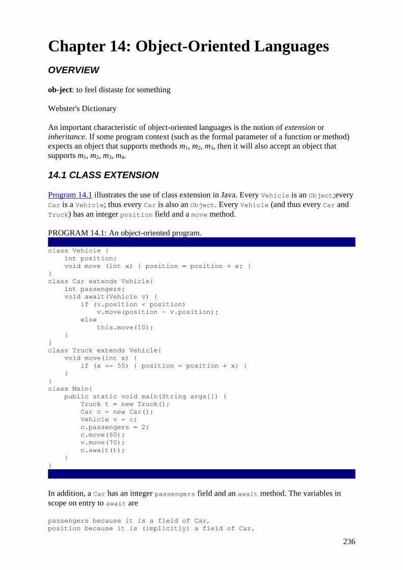
236

Chapter 14: Object-Oriented Languages OVERVIEW

ob-ject: to feel distaste for something


An important characteristic of object-oriented languages is the notion of extension or inheritance. If some program context (such as the formal parameter of a function or method) expects an object that supports methods m1, m2, m3, then it will also accept an object that supports m1, m2, m3, m4.

14.1 CLASS EXTENSION

Program 14.1 illustrates the use of class extension in Java. Every Vehicle is an Object;every Car is a Vehicle; thus every Car is also an Object. Every Vehicle (and thus every Car and Truck) has an integer position field and a move method.

PROGRAM 14.1: An object-oriented program. class Vehicle { int position; void move (int x) { position = position + x; } } class Car extends Vehicle{ int passengers; void await(Vehicle v) { if (v.position < position) v.move(position - v.position); else this.move(10); } } class Truck extends Vehicle{ void move(int x) { if (x <= 55) { position = position + x; } } } class Main{ public static void main(String args[]) { Truck t = new Truck(); Car c = new Car(); Vehicle v = c; c.passengers = 2; c.move(60); v.move(70); c.await(t); } }

In addition, a Car has an integer passengers field and an await method. The variables in scope on entry to await are

passengers because it is a field of Car, position because it is (implicitly) a field of Car,

237

v because it is a formal parameter of await, this because it is (implicitly) a formal parameter of await.

At the call to c.await(t), the truck t is bound to the formal parameter v of the await method. Then when v.move is called, this activates the Truck_move method body, not Vehicle_move.

We use the notation A_m to indicate a method instance m declared within aclass A. This is not part of the Java syntax, it is just for use in discussing the semantics of Java programs. Each different declaration of a method is a different method instance. Two different method instances could have the same method name if, for example, one overrides the other.

14.2 SINGLE INHERITANCE OF DATA FIELDS

To evaluate the expression v.position, where v belongs to class Vehicle, the compiler must generate code to fetch the field position from the object (record) that v points to.

This seems simple enough: The environment entry for variable v contains (among other things) a pointer to the type (class) description of Vehicle; this has a list of fields and their offsets. But at run time the variable v could also contain a pointer to a Car or Truck; where will the position field be in a Car or Truck object?

Single inheritance For single-inheritance languages, in which each class extends just one parent class, the simple technique of prefixing works well. Where B extends A, those fields of B that are inherited from A are laid out in a B record at the beginning, in the same order they appear in A records. Fields of B not inherited from A are placed afterward, as shown in Figure 14.2.

Figure 14.2: Single inheritance of data fields.

METHODS

A method instance is compiled much like a function: It turns into machine code that resides at a particular address in the instruction space. Let us say, for example, that the method instance Truck_move has an entry point at machine-code label Truck_move. In the semantic analysis phase of the compiler, each variable's environment entry contains a pointer to its class descriptor; each class descriptor contains a pointer to its parent class, and also a list of method instances; and each method instance has a machine-code label.

Static methods Some object-oriented languages allow some methods to be declared static. The machine code that executes when c.f() is called depends on the type of the variable c, not the type of the object that c holds. To compile a method-call of the form c.f(), the compiler finds the class of c; let us suppose it is class C. Then it searches in class C for a method f; suppose none is found. Then it searches the parent class of C, class B, for a method f; then the parent class of B; and so on. Suppose in some ancestor class A it finds a static method f; then it can compile a function call to label A_f.

238

Dynamic methods This technique will not work for dynamic methods. If method f in A is a dynamic method, then it might be overridden in some class D which is a subclass of C (see Figure 14.3). But there is no way to tell at compile time if the variable c is pointing to an object of class D (in which case D_f should be called) or class C (in which case A_f should be called).

Figure 14.3: Class descriptors for dynamic method lookup.

To solve this problem, the class descriptor must contain a vector with a method instance for each (nonstatic) method name. When class B inherits from A, the method table starts with entries for all method names known to A, and then continues with new methods declared by B. This is very much like the arrangement of fields in objects with inheritance.

Figure 14.3 shows what happens when class D overrides method f. Although the entry for f is at the beginning of D's method table, as it is also at the beginning of the ancestor class A's method table, it points to a different method-instance label because f has been overridden.

To execute c.f(), where f is a dynamic method, the compiled code must execute these instructions:

1. Fetch the class descriptor d at offset 0 from object c. 2. Fetch the method-instance pointer p from the (constant) f offset of d. 3. Jump to address p, saving return address (that is, call p).

14.3 MULTIPLE INHERITANCE

In languages that permit a class D to extend several parent classes A, B, C (that is, where A is not a subclass of B, or vice versa), finding field offsets and method instances is more difficult. It is impossible to put all the A fields at the beginning of D and to put all the B fields at the beginning of D.

Global graph coloring One solution to this problem is to statically analyze all classes at once, finding some offset for each field name that can be used in every record containing that field. We can model this as a graph-coloring problem: There is a node for each distinct field name, and an edge for any two fields which coexist (perhaps by inheritance) in the same class.[1] The offsets 0, 1, 2;… are the colors. Figure 14.4 shows an example.

Figure 14.4: Multiple inheritance of data fields.

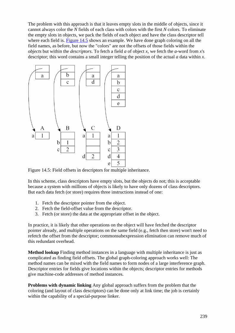
239

The problem with this approach is that it leaves empty slots in the middle of objects, since it cannot always color the N fields of each class with colors with the first N colors. To eliminate the empty slots in objects, we pack the fields of each object and have the class descriptor tell where each field is. Figure 14.5 shows an example. We have done graph coloring on all the field names, as before, but now the "colors" are not the offsets of those fields within the objects but within the descriptors. To fetch a field a of object x, we fetch the a-word from x's descriptor; this word contains a small integer telling the position of the actual a data within x.

Figure 14.5: Field offsets in descriptors for multiple inheritance.

In this scheme, class descriptors have empty slots, but the objects do not; this is acceptable because a system with millions of objects is likely to have only dozens of class descriptors. But each data fetch (or store) requires three instructions instead of one:

1. Fetch the descriptor pointer from the object. 2. Fetch the field-offset value from the descriptor. 3. Fetch (or store) the data at the appropriate offset in the object.

In practice, it is likely that other operations on the object will have fetched the descriptor pointer already, and multiple operations on the same field (e.g., fetch then store) won't need to refetch the offset from the descriptor; commonsubexpression elimination can remove much of this redundant overhead.

Method lookup Finding method instances in a language with multiple inheritance is just as complicated as finding field offsets. The global graph-coloring approach works well: The method names can be mixed with the field names to form nodes of a large interference graph. Descriptor entries for fields give locations within the objects; descriptor entries for methods give machine-code addresses of method instances.

Problems with dynamic linking Any global approach suffers from the problem that the coloring (and layout of class descriptors) can be done only at link time; the job is certainly within the capability of a special-purpose linker.

240

However, many object-oriented systems have the capability to load new classes into a running system; these classes may be extensions (subclasses) of classes already in use. Link-time graph coloring poses many problems for a system that allows dynamic incremental linking.

Hashing Instead of global graph coloring, we can put a hash table in each class descriptor, mapping field names to offsets and method names to method instances. This works well with separate compilation and dynamic linking.

The characters of the field names are not hashed at run time. Instead, each field name a is hashed at compile time to an integer hasha in the range [0, N − 1]. Also, for each field name a unique run-time record (pointer) ptra is made.

Each class descriptor has a field-offset table Ftab of size N containing field-offsets and method instances, and (for purposes of collision detection) a parallel key table Ktab containing field-name pointers. If the class has a field x, then field-offset-table slot number hashx contains the offset for x, and key-table slot number hashx contains the pointer ptrx.

To fetch a field x of object c, the compiler generates code to

1. Fetch the class descriptor d at offset 0 from object c. 2. Fetch the field name f from the address offset d + Ktab + hashx. 3. Test whether f = ptrx; if so 4. Fetch the field offset k from d + Ftab + hashx. 5. Fetch the contents of the field from c + k.

This algorithm has four instructions of overhead, which may still be tolerable. A similar algorithm works for dynamic method-instance lookup.

The algorithm as described does not say what to do if the test at line 3 fails. Any hash-table collision-resolution technique can be used.

[1]Distinct field name does not mean simple equivalence of strings. Each fresh declaration of field or method x (where it is not overriding the x of a parent class) is really a distinct name.

14.4 TESTING CLASS MEMBERSHIP

Some object-oriented languages allow the program to test membership of an object in a class at run time, as summarized in Table 14.6.

Table 14.6. Facilities for type testing and safe casting. Modula-3 Java

Test whether object x belongs class C, or to any subclass of C. ISTYPE(x,C) x instanceof

C

Given a variable x of class C, where x actually points to an object of class D that extends C, yield an expression whose compile-time type is class D.

NARROW(x,D) (D)x

241

Since each object points to its class descriptor, the address of the class descriptor can serve as a "type-tag." However, if x is an instance of D, and D extends C, then x is also an instance of C. Assuming there is no multiple inheritance, a simple way to implement x instanceof C is to generate code that performs the following loop at run time:

goto L1

where t1.super is the superclass (parent class) of class t1.

However, there is a faster approach using a display of parent classes. Assume that the class nesting depth is limited to some constant, such as 20. Reserve a 20-word block in each class descriptor. In the descriptor for a class D whose nesting depth is j, put a pointer to descriptor D in the jth slot, a pointer to D.super in the (j − 1)th slot, a pointer to D.super.super in slot j − 2, andsoonupto Object in slot 0. In all slots numbered greater than j, put nil.

Now, if x is an instance of D, or of any subclass of D, then the jth slot of x's class descriptor will point to the class descriptor D. Otherwise it will not. So x instanceof D requires

1. Fetch the class descriptor d at offset 0 from object c. 2. Fetch the jth class-pointer slot from d. 3. Compare with the class descriptor D.

This works because the class-nesting depth of D is known at compile time.

Type coercions Given a variable c of type C, it is always legal to treat c as any supertype of C - if C extends B, and variable b has type B, then the assignment b ← c is legal and safe.

But the reverse is not true. The assignment c ← b is safe only if b is really (at run time) an instance of C, which is not always the case. If we have b ← new B, c ← b, followed by fetching some field of c that is part of class C but not class B, then this fetch will lead to unpredictable behavior.

Thus, safe object-oriented languages (such as Modula-3 and Java) accompany any coercion from a superclass to a subclass with a run-time type-check that raises an exception unless the run-time value is really an instance of the subclass (e.g., unless b instanceof C).

It is a common idiom to write

Modula-3: Java: IF ISTYPE(b,C) if (b instanceof C) THEN f(NARROW(b,C)) f((C)b) ELSE ... else ...

242

Now there are two consecutive, identical type tests: one explicit (ISTYPE or instanceof) and one implicit (in NARROW or the cast). A good compiler will do enough flow analysis to notice that the then-clause is reached only if b is in fact an instance of C, so that the type-check in the narrowing operation can be eliminated.

C++ is an unsafe object-oriented language. It has a static cast mechanism without run-time checking; careless use of this mechanism can make the program "go wrong" in unpredictable ways. C++ also has dynamic_cast with run-time checking, which is like the mechanisms in Modula-3 and Java.

Typecase Explicit instanceof testing, followed by a narrowing cast to a subclass, is not a wholesome "object-oriented" style. Instead of using this idiom, programmers are expected to use dynamic methods that accomplish the right thing in each subclass. Nevertheless, the test-then-narrow idiom is fairly common.

Modula-3 has a typecase facility that makes the idiom more beautiful and efficient (but not any more "object-oriented"):

TYPECASE expr OF C1 (v1) => S1 | C2 (v2) => S2

⋮ | Cn (vn) => Sn ELSE S0 END

If the expr evaluates to an instance of class Ci, then a new variable vi of type Ci points to the result of the expr, and statement Si is executed. The declaration of vi is implicit in the TYPECASE, and its scope covers only Si.

If more than one of the Ci match (which can happen if, for example, one is a superclass of another), then only the first matching clause is taken. If none of the Ci match, then the ELSE clause is taken (statement S0 is executed).

Typecase can be converted straightforwardly to a chain of else-ifs, with each if doing an instance test, a narrowing, and a local variable declaration. However, if there are very many clauses, then it can take a long time to go through all the else-ifs. Therefore it is attractive to treat it like a case (switch) statement on integers, using an indexed jump (computed goto).

That is, an ordinary case statement on integers:

ML: C, Java: case i switch (i) { of 0 => s0 case 0: s0; break; | 1=> s1 case 1: s1; break; | 2=> s2 case 2: s2; break; | 3=> s3 case 3: s3; break; | 4=> s4 case 4: s4; break; |_=> sd default: sd; }

is compiled as follows: First a range-check comparison is made to ensure that i is within the range of case labels (0-4, in this case); then the address of the ith statement is fetched from the ith slot of a table, and control jumps to si.

243

This approach will not work for typecase, because of subclassing. That is, even if we could make class descriptors be small integers instead of pointers, we cannot do an indexed jump based on the class of the object, because we will miss clauses that match superclasses of that class. Thus, Modula-3 typecase is implemented as a chain of else-ifs.

Assigning integers to classes is not trivial, because separately compiled modules can each define their own classes, and we do not want the integers to clash. But a sophisticated linker might be able to assign the integers at link time.

If all the classes in the typecase were final classes (in the sense used by Java, that they cannot be extended), then this problem would not apply. Modula-3 does not have final classes; and Java does not have typecase. But a clever Java system might be able to recognize a chain of else-ifs that do instanceof tests for a set of final classes, and generate a indexed jump.

14.5 PRIVATE FIELDS AND METHODS

True object-oriented languages can protect fields of objects from direct manipulation by other objects' methods. A private field is one that cannot be fetched or updated from any function or method declared outside the object; a private method is one that cannot be called from outside the object.

Privacy is enforced by the type-checking phase of the compiler. In the symbol table of C, along with each field offset and method offset, is a boolean flag indicating whether the field is private. When compiling the expression c.f() or c.x, it is a simple matter to check that field and reject accesses to private fields from any method outside the object declaration.

There are many varieties of privacy and protection. Different languages allow

• Fields and methods which are accessible only to the class that declares them. • Fields and methods accessible to the declaring class, and to any subclasses of that

class. • Fields and methods accessible only within the same module (package, namespace) as

the declaring class. • Fields that are read-only from outside the declaring class, but writable by methods of

the class.

In general, these varieties of protection can be statically enforced by compiletime type-checking, for class-based languages.

14.6 CLASSLESS LANGUAGES

Some object-oriented languages do not use the notion of class at all. In such a language, each object implements whatever methods and has whatever data fields it wants. Type-checking for such languages is usually dynamic (done at run time) instead of static (done at compile time).

Many objects are created by cloning: copying an existing object (or template object) and then modifying some of the fields. Thus, even in a classless language there will be groups ("pseudo-classes") of similar objects that can share descriptors. When b is created by cloning a, it can share a descriptor with a. Only if a new field is added or a method field is updated (overridden) does b require a new descriptor.

244

The techniques used in compiling classless languages are similar to those for class-based languages with multiple inheritance and dynamic linking: Pseudo-class descriptors contain hash tables that yield field offsets and method instances.

The same kinds of global program analysis and optimization that are used for class-based languages - finding which method instance will be called from a (dynamic) method call site - are just as useful for classless languages.

14.7 OPTIMIZING OBJECT-ORIENTED PROGRAMS

An optimization of particular importance to object-oriented languages (which also benefit from most optimizations that apply to programming languages in general) is the conversion of dynamic method calls to static method-instance calls.

Compared with an ordinary function call, at each method call site there is a dynamic method lookup to determine the method instance. For single-inheritance languages, method lookup takes only two instructions. This seems like a small cost, but:

• Modern machines can jump to constant addresses more efficiently than to addresses fetched from tables. When the address is manifest in the instruction stream, the processor is able to pre-fetch the instruction cache at the destination and direct the instruction-issue mechanism to fetch at the target of the jump. Unpredictable jumps stall the instruction-issue and -execution pipeline for several cycles.

• An optimizing compiler that does inline expansion or interprocedural analysis will have trouble analyzing the consequences of a call if it doesn't even know which method instance is called at a given site.

For multiple-inheritance and classless languages, the dynamic method-lookup cost is even higher.

Thus, optimizing compilers for object-oriented languages do global program analysis to determine those places where a method call is always calling the same method instance; then the dynamic method call can be replaced by a static function call.

For a method call c.f(), where c is of class C, type hierarchy analysis is used to determine which subclasses of C contain methods f that may override C_f. If there is no such method, then the method instance must be C_f.

This idea is combined with type propagation, a form of static dataflow analysis similar to reaching definitions (see Section 17.2). After an assignment c ← new C, the exact class of c is known. This information can be propagated through the assignment d ← c, and so on. When d.f() is encountered, the type-propagation information limits the range of the type hierarchy that might contribute method instances to d.

Suppose a method f defined in class C calls method g on this. But g is a dynamic method and may be overridden, so this call requires a dynamic method lookup. An optimizing compiler may make a different copy of a method instance C_f for each subclass (e.g., D,E) that extends C. Then when the (new copy) D_f calls g, the compiler knows to call the instance D_g without a dynamic method lookup.

245

PROGRAM MiniJava WITH CLASS EXTENSION

Implement class extension in your MiniJava compiler.

FURTHER READING

Dahl and Nygaard's Simula-67 language [Birtwistle et al. 1973] introduced the notion of classes, objects, single inheritance, static methods, instance testing, typecase, and the prefix technique to implement static single inheritance. In addition it had coroutines and garbage collection.

Cohen [1991] suggested the display for constant-time testing of class membership.

Dynamic methods and multiple inheritance appeared in Smalltalk [Goldberg et al. 1983], but the first implementations used slow searches of parent classes to find method instances. Rose [1988] and Connor et al. [1989] discuss fast hash-based field- and method-access algorithms for multiple inheritance. The use of graph coloring in implementing multiple inheritance is due to Dixon et al. [1989]. Lippman [1996] shows how C++-style multiple inheritance is implemented.

Chambers et al. [1991] describe several techniques to make classless, dynamically typed languages perform efficiently: pseudo-class descriptors, multiple versions of method instances, and other optimizations. Diwan et al. [1996] describe optimizations for statically typed languages that can replace dynamic method calls by static function calls.

Conventional object-oriented languages choose a method instance for a call a.f(x,y) based only on the class of the method receiver (a) and not other arguments (x,y). Languages with multimethods [Bobrow et al. 1989] allow dynamic method lookup based on the types of all arguments. This would solve the problem of orthogonal directions of modularity discussed on page 93. Chambers and Leavens [1995] show how to do static type-checking for multimethods; Amiel et al. [1994] and Chen and Turau [1994] show how to do efficient dynamic multimethod lookup.

Nelson [1991] describes Modula-3, Stroustrup [1997] describes C++, and Arnold and Gosling [1996] describe Java.

EXERCISES

• *14.1 A problem with the display technique (as explained on page 290) for testing class membership is that the maximum class-nesting depth N must be fixed in advance, and every class descriptor needs N words of space even if most classes are not deeply nested. Design a variant of the display technique that does not suffer from these problems; it will be a couple of instructions more costly than the one described on page 290.

• 14.2 The hash-table technique for finding field offsets and method instances in the presence of multiple inheritance is shown incompletely on page 289 − the case of f ≠ ptrx is not resolved. Choose a collision-resolution technique, explain how it works, and analyze the extra cost (in instructions) in the case that f = ptrx(no collision) and f ≠ ptrx (collision).

• *14.3 Consider the following class hierarchy, which contains five method-call sites. The task is to show which of the method-call sites call known method instances, and

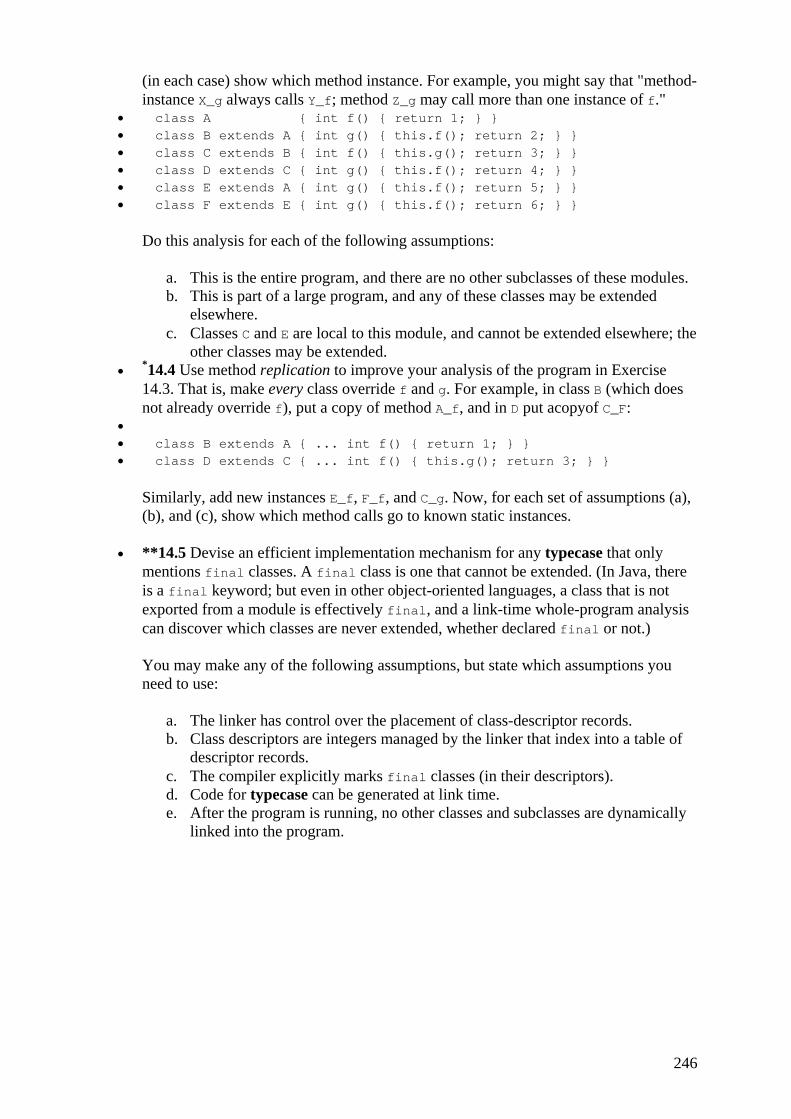
246

(in each case) show which method instance. For example, you might say that "method-instance X_g always calls Y_f; method Z_g may call more than one instance of f."

• class A { int f() { return 1; } } • class B extends A { int g() { this.f(); return 2; } } • class C extends B { int f() { this.g(); return 3; } } • class D extends C { int g() { this.f(); return 4; } } • class E extends A { int g() { this.f(); return 5; } } • class F extends E { int g() { this.f(); return 6; } }

Do this analysis for each of the following assumptions:

a. This is the entire program, and there are no other subclasses of these modules. b. This is part of a large program, and any of these classes may be extended

elsewhere. c. Classes C and E are local to this module, and cannot be extended elsewhere; the

other classes may be extended. • *14.4 Use method replication to improve your analysis of the program in Exercise

14.3. That is, make every class override f and g. For example, in class B (which does not already override f), put a copy of method A_f, and in D put acopyof C_F:

• • class B extends A { ... int f() { return 1; } } • class D extends C { ... int f() { this.g(); return 3; } }

Similarly, add new instances E_f, F_f, and C_g. Now, for each set of assumptions (a), (b), and (c), show which method calls go to known static instances.

• **14.5 Devise an efficient implementation mechanism for any typecase that only mentions final classes. A final class is one that cannot be extended. (In Java, there is a final keyword; but even in other object-oriented languages, a class that is not exported from a module is effectively final, and a link-time whole-program analysis can discover which classes are never extended, whether declared final or not.)

You may make any of the following assumptions, but state which assumptions you need to use:

a. The linker has control over the placement of class-descriptor records. b. Class descriptors are integers managed by the linker that index into a table of

descriptor records. c. The compiler explicitly marks final classes (in their descriptors). d. Code for typecase can be generated at link time. e. After the program is running, no other classes and subclasses are dynamically

linked into the program.

247

Appendix A: MiniJava Language Reference Manual MiniJava is a subset of Java. The meaning of a MiniJava program is given by its meaning as a Java program. Overloading is not allowed in MiniJava. The MiniJava statement System.out.println( …); can only print integers. The MiniJava expression e.length only applies to expressions of type int[].

A.1 LEXICAL ISSUES

Identifiers: An identifier is a sequence of letters, digits, and underscores, starting with a letter. Uppercase letters are distinguished from lowercase. In this appendix the symbol id stands for an identifier.

Integer literals: A sequence of decimal digits is an integer constant that denotes the corresponding integer value. In this appendix the symbol INTEGER_LITERAL stands for an integer constant.

Binary operators: A binary operator is one of

&& < + - *

In this appendix the symbol op stands for a binary operator.

Comments: A comment may appear between any two tokens. There are two forms of comments: One starts with /*, ends with */, and may be nested; another begins with // and goes to the end of the line.

A.2 GRAMMAR

In the MiniJava grammar, we use the notation N*, where N is a nonterminal, to mean 0, 1, or more repetitions of N.

GRAMMAR A.2 Program → MainClass ClassDecl* MainClass → class id { public static void main ( String [] id ) { Statement }}

ClassDecl → class id { VarDecl* MethodDecl* } → class id extends id { VarDecl* MethodDecl* } VarDecl → Type id ; MethodDecl → public Type id ( FormalList ) { VarDecl* Statement* return Exp ;}

FormalList → Type id FormalRest* → FormalRest →, Type id Type → int [] → boolean → int

248

→ id Statement → { Statement* } → if ( Exp ) Statement else Statement → while ( Exp ) Statement → System.out.println ( Exp ) ; → id = Exp ; → id [ Exp ]= Exp ; Exp → Exp op Exp → Exp [ Exp ] → Exp . length → Exp . id ( ExpList ) → INTEGER LITERAL → true → false → id → this → new int [ Exp ] → new id () → ! Exp → ( Exp ) ExpList → Exp ExpRest* → ExpRest → ,Exp

A.3 SAMPLE PROGRAM class Factorial { public static void main(String[] a) { System.out.println(new Fac().ComputeFac(10)); } } class Fac { public int ComputeFac(int num) { int num_aux; if (num < 1) num_aux = 1; else num_aux = num * (this.ComputeFac(num-1)); return num_aux; }

1 Modern Compiler Implementation in Java, Second Edition ...

Documents