1 Managing Flow Variability: Safety Inventory Forecasts Depend on: (a) Historical Data and (b) Market Intelligence. Demand Forecasts and Forecast Errors.

1

Managing Flow Variability: Safety Inventory


Forecasts Depend on: (a) Historical Data and (b) Market Intelligence.

Demand Forecasts and Forecast Errors

Safety Inventory and Service Level

Optimal Service Level – The Newsvendor Problem

Lead Time Demand Variability

Pooling Efficiency through Aggregation

Shortening the Forecast Horizon

Levers for Reducing Safety Inventory

2


Four Characteristics of Forecasts

Forecasts are usually (always) inaccurate (wrong). Because of random noise.

Forecasts should be accompanied by a measure of forecast error. A measure of forecast error (standard deviation) quantifies the manager’s degree of confidence in the forecast.

Aggregate forecasts are more accurate than individual forecasts. Aggregate forecasts reduce the amount of variability – relative to the aggregate mean demand. StdDev of sum of two variables is less than sum of StdDev of the two variables.

Long-range forecasts are less accurate than short-range forecasts. Forecasts further into the future tends to be less accurate than those of more imminent events. As time passes, we get better information, and make better prediction.

3


Demand During Lead Time is Variable N(μ,σ)

Demand of sand during lead time has an average of 50 tons.Standard deviation of demand during lead time is 5 tonsAssuming that the management is willing to accept a risk

no more that 5%.

4


Forecast and a Measure of Forecast ErrorForecasts should be accompanied by a measure of forecast error

5


Time

Inve

ntor

y

Demand During Lead Time

Demand during LT

Lead Time

6


LT

ROP when Demand During Lead Time is Fixed

7


LT

Demand During Lead Time is Variable

8


Inventory

Time

Demand During Lead Time is Variable

9


Average demandduring lead time

A large demandduring lead time

ROP

Time

Qu

an

tity

Safety stock reduces risk ofstockout during lead time

Safety Stock

Safety stock

LT

10


ROP

Time

Qu

an

tity

Safety Stock

LT

11


Re-Order Point: ROP

Demand during lead time has Normal distribution.

We can accept some risk of being out of stock, but we usually like a risk of less than 50%.

If we order when the inventory on hand is equal to the average demand during the lead time; then there is 50% chance that the demand during lead time is less than our inventory.

However, there is also 50% chance that the demand during lead time is greater than our inventory, and we will be out of stock for a while.We usually do not like 50% probability of stock out

12


ROP

Risk of astockout

Service level

Probability ofno stockout

Safetystock

0 z

Quantity

z-scale

Safety Stock and ROP

Each Normal variable x is associated with a standard Normal Variable z

Averagedemand

x is Normal (Average x , Standard Deviation x) z is Normal (0,1)

13


z Values

SL z value0.9 1.280.95 1.650.99 2.33

ROP

Risk of astockout

Service level


Safetystock

0 z

Quantity

z-scale

Averagedemand

There is a table for z which tells us a) Given any probability of not exceeding z. What is the value of z b) Given any value for z. What is the probability of not exceeding z

14


μ and σ of Demand During Lead Time

Demand of sand during lead time has an average of 50 tons.Standard deviation of demand during lead time is 5 tons.Assuming that the management is willing to accept a risk no

more that 5%. Find the re-order point.

What is the service level.Service level = 1-risk of stockout = 1-.05 = .95Find the z value such that the probability of a standard

normal variable being less than or equal to z is .95Go to normal table, look inside the table. Find a probability

close to .95. Read its z from the corresponding row and column.

15


The table will give you z

Given a 95% SL95% Probability

Page 319: Normal table

Up to the first digitafterdecimal

Second digitafter decimal

Probability

z

1.6

0.05

Z = 1.65

z Value using Table

16


The standard Normal Distribution F(z)

z 0.00 0.01 0.02 0.03 0.04 0.05 0.06 0.07 0.08 0.090.0 0.5000 0.5040 0.5080 0.5120 0.5160 0.5199 0.5239 0.5279 0.5319 0.53590.1 0.5398 0.5438 0.5478 0.5517 0.5557 0.5596 0.5636 0.5675 0.5714 0.57530.2 0.5793 0.5832 0.5871 0.5910 0.5948 0.5987 0.6026 0.6064 0.6103 0.61410.3 0.6179 0.6217 0.6255 0.6293 0.6331 0.6368 0.6406 0.6443 0.6480 0.65170.4 0.6554 0.6591 0.6628 0.6664 0.6700 0.6736 0.6772 0.6808 0.6844 0.68790.5 0.6915 0.6950 0.6985 0.7019 0.7054 0.7088 0.7123 0.7157 0.7190 0.72240.6 0.7257 0.7291 0.7324 0.7357 0.7389 0.7422 0.7454 0.7486 0.7517 0.75490.7 0.7580 0.7611 0.7642 0.7673 0.7704 0.7734 0.7764 0.7794 0.7823 0.78520.8 0.7881 0.7910 0.7939 0.7967 0.7995 0.8023 0.8051 0.8078 0.8106 0.81330.9 0.8159 0.8186 0.8212 0.8238 0.8264 0.8289 0.8315 0.8340 0.8365 0.83891.0 0.8413 0.8438 0.8461 0.8485 0.8508 0.8531 0.8554 0.8577 0.8599 0.86211.1 0.8643 0.8665 0.8686 0.8708 0.8729 0.8749 0.8770 0.8790 0.8810 0.88301.2 0.8849 0.8869 0.8888 0.8907 0.8925 0.8944 0.8962 0.8980 0.8997 0.90151.3 0.9032 0.9049 0.9066 0.9082 0.9099 0.9115 0.9131 0.9147 0.9162 0.91771.4 0.9192 0.9207 0.9222 0.9236 0.9251 0.9265 0.9279 0.9292 0.9306 0.93191.5 0.9332 0.9345 0.9357 0.9370 0.9382 0.9394 0.9406 0.9418 0.9429 0.94411.6 0.9452 0.9463 0.9474 0.9484 0.9495 0.9505 0.9515 0.9525 0.9535 0.95451.7 0.9554 0.9564 0.9573 0.9582 0.9591 0.9599 0.9608 0.9616 0.9625 0.96331.8 0.9641 0.9649 0.9656 0.9664 0.9671 0.9678 0.9686 0.9693 0.9699 0.97061.9 0.9713 0.9719 0.9726 0.9732 0.9738 0.9744 0.9750 0.9756 0.9761 0.97672.0 0.9772 0.9778 0.9783 0.9788 0.9793 0.9798 0.9803 0.9808 0.9812 0.98172.1 0.9821 0.9826 0.9830 0.9834 0.9838 0.9842 0.9846 0.9850 0.9854 0.98572.2 0.9861 0.9864 0.9868 0.9871 0.9875 0.9878 0.9881 0.9884 0.9887 0.98902.3 0.9893 0.9896 0.9898 0.9901 0.9904 0.9906 0.9909 0.9911 0.9913 0.99162.4 0.9918 0.9920 0.9922 0.9925 0.9927 0.9929 0.9931 0.9932 0.9934 0.99362.5 0.9938 0.9940 0.9941 0.9943 0.9945 0.9946 0.9948 0.9949 0.9951 0.99522.6 0.9953 0.9955 0.9956 0.9957 0.9959 0.9960 0.9961 0.9962 0.9963 0.99642.7 0.9965 0.9966 0.9967 0.9968 0.9969 0.9970 0.9971 0.9972 0.9973 0.99742.8 0.9974 0.9975 0.9976 0.9977 0.9977 0.9978 0.9979 0.9979 0.9980 0.99812.9 0.9981 0.9982 0.9982 0.9983 0.9984 0.9984 0.9985 0.9985 0.9986 0.99863.0 0.9987 0.9987 0.9987 0.9988 0.9988 0.9989 0.9989 0.9989 0.9990 0.99903.1 0.9990 0.9991 0.9991 0.9991 0.9992 0.9992 0.9992 0.9992 0.9993 0.99933.2 0.9993 0.9993 0.9994 0.9994 0.9994 0.9994 0.9994 0.9995 0.9995 0.99953.3 0.9995 0.9995 0.9995 0.9996 0.9996 0.9996 0.9996 0.9996 0.9996 0.9997

F(z)

z0

F(z) = Prob( N(0,1) < z)

17


Relationship between z and Normal Variable x

ROP

Risk of astockout

Service level


Safetystock

0 z

Quantity

z-scale

Averagedemand

z = (x-Average x)/(Standard Deviation of x)x = Average x +z (Standard Deviation of x)μ = Average x σ = Standard Deviation of x

x = μ +z σ

18


Relationship between z and Normal Variable ROP

ROP

Risk of astakeout

Service level


Safetystock

0 z

Quantity

z-scale

Averagedemand

LTD = Lead Time DemandROP = Average LTD +z (Standard Deviation of LTD) ROP = LTD+zσLTD ROP = LTD + Isafety

19


Demand During Lead Time is Variable N(μ,σ)

Demand of sand during lead time has an average of 50 tons.Standard deviation of demand during lead time is 5 tonsAssuming that the management is willing to accept a risk

no more that 5%.

Compute safety stockIsafety = zσLTD Isafety = 1.64 (5) = 8.2

ROP = LTD + Isafety

ROP = 50 + 1.64(5) = 58.2

z = 1.65

20


Service Level for a given ROP

SL = Prob (LTD ≤ ROP)

LTD is normally distributed LTD = N(LTD, LTD ).

ROP = LTD + zσLTD ROP = LTD + Isafety I safety = z LTD

At GE Lighting’s Paris warehouse, LTD = 20,000, LTD = 5,000

The warehouse re-orders whenever ROP = 24,000

I safety = ROP – LTD = 24,000 – 20,000 = 4,000

I safety = z LTD z = I safety / LTD = 4,000 / 5,000 = 0.8

SL= Prob (Z ≤ 0.8) from Appendix II SL= 0.7881

21


Excel: Given z, Compute Probability

22


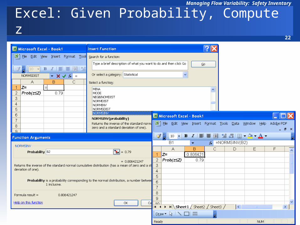
Excel: Given Probability, Compute z

23


Demand of sand has an average of 50 tons per week.Standard deviation of the weekly demand is 3 tons.Lead time is 2 weeks.Assuming that the management is willing to accept a risk

no more that 10%. Compute the Reorder Point

μ and σ of demand per period and fixed LT

24



R: demand rate per period (a random variable) R: Average demand rate per periodσR: Standard deviation of the demand rate per period

L: Lead time (a constant number of periods)

LTD: demand during the lead time (a random variable) LTD: Average demand during the lead time σLTD: Standard deviation of the demand during lead time

25



A random variable R: N(R, σR) repeats itself L times during the lead time. The summation of these L random variables R, is a random variable LTD

LRLTD

RLTD L

If we have a random variable LTD which is equal to summation of L random variables RLTD = R1+R2+R3+…….+RL

Then there is a relationship between mean and standard deviation of the two random variables

22RLTD L

26


RLTD L

LRLTD

Demand of sand has an average of 50 tons per week.Standard deviation of the weekly demand is 3 tons.Lead time is 2 weeks.Assuming that the management is willing to accept a risk

no more that 10%.


24.4)3(2

100)50(2

RLTD L

LTD

Isafety = zσLTD = 1.28(4.24) = 5.43

ROP = 100 + 5.43

z = 1.28, R = 50, σR = 3, L = 2

27


Lead Time Variable, Demand fixed

Demand of sand is fixed and is 50 tons per week.The average lead time is 2 weeks.Standard deviation of lead time is 0.5 week.Assuming that the management is willing to accept a risk

no more that 10%. Compute ROP and Isafety.

28


μ and σ of lead time and fixed Demand per period

L: lead time (a random variable) L: Average lead timeσL: Standard deviation of the lead time

RL

RL

R: Demand per period (a constant value)


29



A random variable L: N(L, σL) is multiplied by a constant R and generates the random variable LTD.

If we have a random variable LTD which is equal to a constant R times a random variables LLTD = RLThen there is a relationship between mean and standard deviation of the two random variables

LRLTD 222LLTD R

RL

RL

LLTD R

30


Variable R fixed L…………….Variable L fixed R

LLTD

LLTD

R

R

LRLTD

222

RL

RL

RLTD

RLTD

L

L

LRLTD

22

R R R R R

L

R+R+R+R+R

31


Lead Time Variable, Demand fixed

Demand of sand is fixed and is 50 tons per week.The average lead time is 2 weeks.Standard deviation of lead time is 0.5 week.Assuming that the management is willing to accept a risk no

more that 10%. Compute ROP and Isafety.z = 1.28, L = 2 weeks, σL = 0.5 week, R = 50 per week

25)5.0(50

100)2(50

LLTD R

LRLTD

Isafety = zσLTD = 1.28(25) = 32

ROP = 100 + 32

32


Both Demand and Lead Time are Variable

R: demand rate per period R: Average demand rateσR: Standard deviation of demand

L: lead time L: Average lead timeσL: Standard deviation of the lead time


LRLTD RL

LRLTD

2

33


Optimal Service Level: The Newsvendor Problem

Cost of Holding Extra Inventory

Improved Service

Optimal Service Level under uncertainty

The Newsvendor Problem

The decision maker balances the expected costs of ordering too much with the expected costs of ordering too little to determine the optimal order quantity.

How do we choose what level of service a firm should offer?

34



Demand Probability of Demand100 0.02110 0.05120 0.08130 0.09140 0.11150 0.16160 0.2170 0.15180 0.08190 0.05200 0.01

Cost =1800, Sales Price = 2500, Salvage Price = 1700Underage Cost = 2500-1800 = 700, Overage Cost = 1800-1700 = 100

What is probability of demand to be equal to 130?What is probability of demand to be less than or equal to 140?What is probability of demand to be greater than 140?What is probability of demand to be equal to 133?

35



Demand Probability of Demand100 0.002101 0.002102 0.002103 0.002104 0.002105 0.002106 0.002107 0.002108 0.002109 0.002

What is probability of demand to be equal to 116?What is probability of demand to be less than or equal to 160?What is probability of demand to be greater than 116?What is probability of demand to be equal to 13.3?

Demand Probability of Demand110 0.005111 0.005112 0.005113 0.005114 0.005115 0.005116 0.005117 0.005118 0.005119 0.005

36



What is probability of demand to be equal to 130?What is probability of demand to be less than or equal to 140?What is probability of demand to be greater than 140?What is probability of demand to be equal to 133?

Average Demand Probability of Demand100 0.02110 0.05120 0.08130 0.09140 0.11150 0.16160 0.2170 0.15180 0.08190 0.05200 0.01

37


Compute the Average Demand

r P( R =r)

100 0.02110 0.05120 0.08130 0.09140 0.11150 0.16160 0.2170 0.15180 0.08190 0.05200 0.01

)(r Demand AverageN

1ii irRP

Average Demand = +100×0.02 +110×0.05+120×0.08 +130×0.09+140×0.11 +150×0.16+160×0.20 +170×0.15 +180×0.08 +190×0.05+200×0.01Average Demand = 151.6

How many units should I have to sell 151.6 units (on average)? How many units do I sell (on average) if I have 100 units?

38


Suppose I have ordered 140 Unities.On average, how many of them are sold? In other words, what is

the expected value of the number of sold units?

When I can sell all 140 units? I can sell all 140 units if R≥ 140Prob(R≥ 140) = 0.76The the expected number of units sold –for this part- is(0.76)(140) = 106.4Also, there is 0.02 probability that I sell 100 units 2 unitsAlso, there is 0.05 probability that I sell 110 units5.5Also, there is 0.08 probability that I sell 120 units 9.6Also, there is 0.09 probability that I sell 130 units 11.7106.4 + 2 + 5.5 + 9.6 + 11.7 = 135.2

Deamand (r) 100 110 120 130 140 150 160 170 180 190 200Porbability 0.02 0.05 0.08 0.09 0.11 0.16 0.20 0.15 0.08 0.05 0.01Prob(R ≥ r) 1.00 0.98 0.93 0.85 0.76 0.65 0.49 0.29 0.14 0.06 0.01

39


Suppose I have ordered 140 Unities.On average, how many of them are salvaged? In other words,

what is the expected value of the number of sold units?

0.02 probability that I sell 100 units. In that case 40 units are salvaged 0.02(40) = .80.05 probability to sell 110 30 salvage 0.05(30)= 1.5 0.08 probability to sell 120 30 salvage 0.08(20) = 1.60.09 probability to sell 130 30 salvage 0.09(10) =0.9 0.8 + 1.5 + 1.6 + 0.9 = 4.8

Total number Solved 135.2 @ 700 = 94640Total number Salvaged 4.8 @ -100 = -480Expected Profit = 94640 – 480 = 94,160

Deamand (r) 100 110 120 130 140 150 160 170 180 190 200Porbability 0.02 0.05 0.08 0.09 0.11 0.16 0.20 0.15 0.08 0.05 0.01Prob(R ≥ r) 1.00 0.98 0.93 0.85 0.76 0.65 0.49 0.29 0.14 0.06 0.01

40


Cumulative Probabilities

P(R=r) P(R≤r) P(R≥r) Sold Salvage Salvage Sales Total100 0.02 0.02 1 100 0 70000 0 70000110 0.05 0.07 0.98 109.8 0.2 76860 20 76840120 0.08 0.15 0.93 119.1 0.9 83370 90 83280130 0.09 0.24 0.85 127.6 2.4 89320 240 89080140 0.11 0.35 0.76 135.2 4.8 94640 480 94160150 0.16 0.51 0.65 141.7 8.3 99190 830 98360160 0.2 0.71 0.49 146.6 13.4 102620 1340 101280170 0.15 0.86 0.29 149.5 20.5 104650 2050 102600180 0.08 0.94 0.14 150.9 29.1 105630 2910 102720190 0.05 0.99 0.06 151.5 38.5 106050 3850 102200200 0.01 1 0.01 151.6 48.4 106120 4840 101280

RevenueUnitsProbabilities

41


Number of Units Sold, Salvages

P(R=r) P(R≤r) P(R≥r) Sold Salvage Salvage Sales Total100 0.02 0.02 1 100 0 70000 0 70000110 0.05 0.07 0.98 109.8 0.2 76860 20 76840120 0.08 0.15 0.93 119.1 0.9 83370 90 83280130 0.09 0.24 0.85 127.6 2.4 89320 240 89080140 0.11 0.35 0.76 135.2 4.8 94640 480 94160150 0.16 0.51 0.65 141.7 8.3 99190 830 98360160 0.2 0.71 0.49 146.6 13.4 102620 1340 101280170 0.15 0.86 0.29 149.5 20.5 104650 2050 102600180 0.08 0.94 0.14 150.9 29.1 105630 2910 102720190 0.05 0.99 0.06 151.5 38.5 106050 3850 102200200 0.01 1 0.01 151.6 48.4 106120 4840 101280


42


Total Revenue for Different Ordering Policies

P(R=r) P(R≤r) P(R≥r) Sold Salvage Sales Salvage Total100 0.02 0.02 1 100 0 70000 0 70000110 0.05 0.07 0.98 109.8 0.2 76860 20 76840120 0.08 0.15 0.93 119.1 0.9 83370 90 83280130 0.09 0.24 0.85 127.6 2.4 89320 240 89080140 0.11 0.35 0.76 135.2 4.8 94640 480 94160150 0.16 0.51 0.65 141.7 8.3 99190 830 98360160 0.2 0.71 0.49 146.6 13.4 102620 1340 101280170 0.15 0.86 0.29 149.5 20.5 104650 2050 102600180 0.08 0.94 0.14 150.9 29.1 105630 2910 102720190 0.05 0.99 0.06 151.5 38.5 106050 3850 102200200 0.01 1 0.01 151.6 48.4 106120 4840 101280


43


Net Marginal Benefit:

Net Marginal Cost:

MB = p – c

MC = c - v

MB = $2,500 - $1,800 = $700

MC = $1,800 - $1,700 = $100

Analytical Solution for the Optimal Service Level

Suppose I have ordered Q units.

What is the expected cost of ordering one more units?

What is the expected benefit of ordering one more units?

If I have ordered one unit more than Q units, the probability of not selling that extra unit is if the demand is less than or equal to Q. Since we have P( R ≤ Q).

The expected marginal cost =MC× P( R ≤ Q)

If I have ordered one unit more than Q units, the probability of selling that extra unit is if the demand is greater than Q. We know that P(R>Q) = 1- P( R ≤ Q).

The expected marginal benefit = MB× [1-Prob.( R ≤ Q)]

44


As long as expected marginal cost is less than expected marginal profit we buy the next unit. We stop as soon as: Expected marginal cost ≥ Expected marginal profit

MC×Prob(R ≤ Q*) ≥ MB× [1 – Prob(R ≤ Q*)]

MB

MB MCProb(R ≤ Q*) ≥

In a continuous model: SL* = Prob(R ≤ Q*) = MB

MB MC


$700* 0.875

$700 $100

MBSL

MB MC

If we assume demand is normally distributed, What quantity corresponds to this service level ?

45



* 151.6 1.15 22.44 177.41RQ R z

* RQ R z

-4 -3 -2 -1 0 1 2 3 40

0.05

0.1

0.15

0.2

0.25

0.3

0.35

0.4Probability Less than Upper Bound is 0.87493

Den

sity

Critical Value (z)

z = 1.15

46


Aggregate Forecast is More Accurate than Individual Forecasts

-5

-3

-1

1

3

5

-15

-10

-5

0

5

10

15

Demand forecast error for 5 productsMonth P1 P2 P3 P4 P5 Total1 2 4 -3 4 -2 52 0 0 5 0 1 63 2 5 -2 1 0 64 -1 2 -4 1 -2 -45 1 -4 -4 4 3 06 -2 -1 4 5 1 77 4 -5 0 5 -5 -18 -2 2 2 0 -4 -29 -4 1 1 4 3 510 -1 -1 -4 -2 4 -411 4 1 3 2 0 1012 2 0 -4 -3 2 -313 -4 -1 2 -1 -4 -814 0 -5 4 5 -2 215 -5 4 4 0 -4 -116 4 2 2 1 3 1217 -3 2 -2 5 -3 -118 3 1 -3 -1 3 319 2 3 -3 -5 3 020 0 -3 1 -1 -4 -721 -3 4 -4 0 5 222 4 1 -5 4 0 423 0 -4 -5 0 -5 -1424 -2 0 -2 -4 -2 -1025 2 5 -2 5 -1 926 4 5 5 0 1 1527 2 1 4 1 -1 728 0 -3 3 0 -2 -229 3 -2 -1 -1 -4 -530 -2 1 -4 -4 0 -9

-15

-10

-5

0

5

10

15

Demand forecast error for 5 productsMonth P1 P2 P3 P4 P5 Total1 2 4 -3 4 -2 52 0 0 5 0 1 63 2 5 -2 1 0 64 -1 2 -4 1 -2 -45 1 -4 -4 4 3 06 -2 -1 4 5 1 77 4 -5 0 5 -5 -18 -2 2 2 0 -4 -29 -4 1 1 4 3 510 -1 -1 -4 -2 4 -411 4 1 3 2 0 1012 2 0 -4 -3 2 -313 -4 -1 2 -1 -4 -814 0 -5 4 5 -2 215 -5 4 4 0 -4 -116 4 2 2 1 3 1217 -3 2 -2 5 -3 -118 3 1 -3 -1 3 319 2 3 -3 -5 3 020 0 -3 1 -1 -4 -721 -3 4 -4 0 5 222 4 1 -5 4 0 423 0 -4 -5 0 -5 -1424 -2 0 -2 -4 -2 -1025 2 5 -2 5 -1 926 4 5 5 0 1 1527 2 1 4 1 -1 728 0 -3 3 0 -2 -229 3 -2 -1 -1 -4 -530 -2 1 -4 -4 0 -9

-15

-10

-5

0

5

10

15

47


Physical Centralization

Physical Centralization: the firm consolidates all its warehouses in one

location from which is can serve all customers.

Example: Two warehouses. Demand in the two ware houses are independent.

Both warehouses have the same distribution for their lead time demand.

LTD1: N(LTD, σLTD ) LTD2: N(LTD, σLTD )

Both warehouses have identical service levels

To provide desired SL, each location must carry Isafety = zσLTD

z is determined by the desired service level

The total safety inventory in the decentralized system is

LTDDSafety zI 2

48


Independent Lead time demands at two locations

LTDC = LTD1 + LTD2 LTDC = LTD + LTD = 2 LTD

LTDLTDLTDC

LTDVar 222 2 LTDCLTD 2

LTDCSafety zI 2 LTD

DSafety zI 2

GE lighting operating 7 warehouses. A warehouse with average lead

time demand of 20,000 units with a standard deviation of 5,000 units

and a 95% service level needs to carry a safety inventory of

Isafety = 1.65×5000= 8250

750,57250,87 DsafetyI 827,215000765.1 C

safetyI

Decrease in safety inventory by a factor of 65.27

Centralization reduced the safety inventory by a factor of 1/√2

49


independent Lead time demands at N locations

Centralization of N locations: LTDcsafety NzI

Independent demand in N locations: Total safety inventory to

provide a specific SL increases not by N but by √N

If centralization of stocks reduces inventory, why doesn’t everybody do it?

– Longer response time

– Higher shipping cost

– Less understanding of customer needs

– Less understanding of cultural, linguistics, and regulatory barriers

These disadvantages my reduce the demand.

50


Dependent Demand

Does centralization offer similar

benefits when demands in

multiple locations are correlated?

LTD1 and LTD2 are statistically

identically distributed but correlated

with a correlation coefficient of ρ .

LTDLTDLTDLTDCLTD 2)( 222

LTDCLTD )1(2

0

20

40

60

80

100

120

0 10 20 30 40 50 60 70 80 90 100

No Correlation: ρ close to 0

LTDLTDLTDLTDCLTD

22222 )1(22)(

LTDCsafety zI )1(2

51


+ Correlation, + Perfect Correlation

0

20

40

60

80

100

120

0 10 20 30 40 50 60 70 80 90 100

0

20

40

60

80

100

120

0 10 20 30 40 50 60 70 80 90 100

0

10

20

30

40

50

60

70

80

90

100

0 10 20 30 40 50 60 70 80 90 100

Negative Correlation: ρ close to -1

Positive Correlation: ρ close to 1

Perfect Negative Correlation: ρ = -1

0

10

20

30

40

50

60

70

80

90

100

0 10 20 30 40 50 60 70 80 90 100

Perfect Positive Correlation: ρ = +1

52


Correlation

LTDDsafety zI 2

)1/(2)1(2/2

The safety inventory in the two-location decentralized system is larger

than in the centralized system by a factor of

If demand is positively fully correlated, ρ = 1, centralization offers no

benefits in the reduction of safety inventory

Benefits of centralization increases as the demand on the two locations

become negatively correlated. The best case is = -1, where we do not

need safety inventory at all

LTDCsafety zI )1(2

53


Principle of Aggregation and Pooling Inventory

Inventory benefits due to principle of aggregation.

Statistics: Standard deviation of sum of random variables is less than

the sum of the individual standard deviations.

Physical consolidation is not essential, as long as available inventory

is shared among various locations Pooling Inventory

– Virtual Centralization

– Specialization

– Component Commonality

– Delayed Differentiation

– Product Substitution

54


Virtual Centralization

Location A

Exceeds Available stock

1. Information about product demand and availability must be available

at both locations

2. Shipping the product from one location to a customer at another

location must be fast and cost effective

Location B

Less than Available stock

Virtual Centralization: inventory pooling in a network of locations is facilitated using

information regarding availability of goods and subsequent transshipment of goods between

locations to satisfy demand.

Pooling is achieved by keeping the inventories at decentralized locations.

55


Specialization, Substitution

Demand for both products exist in both locations. But a large portion of demand

for P1 is in location A, while a large portion of demand for P2 is in location B.

Both locations keep average inventory.

Safety inventory is kept only in the specialized warehouse

Location A

Product P1

Location B

Product P2

One other possibility to deal with variability is product substitution.

56


Component Commonality

Up to now we have discussed aggregating demand across various geographic

locations, either physical or virtual

Aggregating demand across various products has the same benefits.

Computer manufacturers: offer a wide range of models, but few components,

CPU, RMA, HD, CD/DVD drive, are used across product lines.

Replace Make-to-stock with make Make-to-Order

Commonality + MTO:

Commonality: Safety inventory of the common components much less than

safety inventory of unique components stored separately.

MTO: Inventory cost is computed in terms of WIP cost not in terms of

finished good cost (which is higher).

57


Postponement (Delayed Differentiation)

Forecasting Characteristic: Forecasts further into the future tends to be

less accurate than those of more imminent events.

Since shorter-range forecasts are more accurate, operational decisions

will be more effective if supply is postponed closer to the point of

actual demand.

Two Alternative processes (each activity takes one week)

Alternative A: (1) Coloring the fabric, (2) assembling T-shirts

Alternative B: (1) Assembling T-shirts, (2) coloring the fabric

No changes in flow time. Alternative B postponed the color difference

until one week closer to the time of sale. Takes advantage of the

forecasting characteristic: short-Range forecast more accurate.

58


Postponement (Delayed Differentiation)

Two advantages: Taking advantage of two demand forecasting

characteristics Commonality Advantage: At week 0; Instead of forecast for each

individual item, we forecast for aggregates item – uncolored T-shirt. Forecast for aggregate demand is more accurate than forecast for individual item. It is easier to more accurately forecast total demand for different colored T-shirts for next week than the week after the next.

Postponement Advantage: Instead of forecasting for each individual items two weeks ahead, we do it at week 1. Shorter rang forecasts are more accurate. It is easier to more accurately forecast demand for different colored T-shirts for next week than the week after the next.

59


Lessons Learned

Levels for Reducing Safety Capacity

Reduce demand variability through improved forecasting

Reduce replenishment lead time

Reduce variability in replenishment lead time

Pool safety inventory for multiple locations or products

Exploit product substitution

Use common components

Postpone product-differentiation processing until closer to the

point of actual demand

1 Managing Flow Variability: Safety Inventory Forecasts Depend on: (a) Historical Data and (b) Market Intelligence. Demand Forecasts and Forecast Errors.

Documents