1 LML: Defect Lecture © 2005 Stevens Institute of Technology All Rights Reserved Software Engineering Metrics Linda M. Laird “In Praise of Defects” Stevens.

LML: Defect Lecture © 2005 Stevens Institute of Technology

All Rights Reserved1

Software Engineering Metrics

Linda M. Laird

“In Praise of Defects”

Stevens Institute of Technology



Some Quotations “If debugging is the process of removing bugs, then

programming must be the process of putting them in.” Unknown

“No software system of any realistic size is ever completely debugged --- that is, error free.” Edward Yourdon and Larry Constantine[i]

“…defects do follow a Rayleigh pattern, the same as effort, cost, and code constructed. This curve can be projected before the main build begins; it can be finely tuned. It is the key ingredient for the statistical control of software reliability.” Lawrence H. Putnam and Ware Myers

[i] Yourdon and Constantine, Structured Design: Fundamentals of a Discipline of Computer Program and Systems Design, Prentice-Hall, Englewood Cliffs, NJ, 1979



Some Questions:

Your system has no reported field defects. It was released six months ago. Is it time to break out the champagne?

You are building a commercial application. Your CEO, who is very dedicated to quality, directs you to find and fix 99% of the bugs before you ship. What is your response?



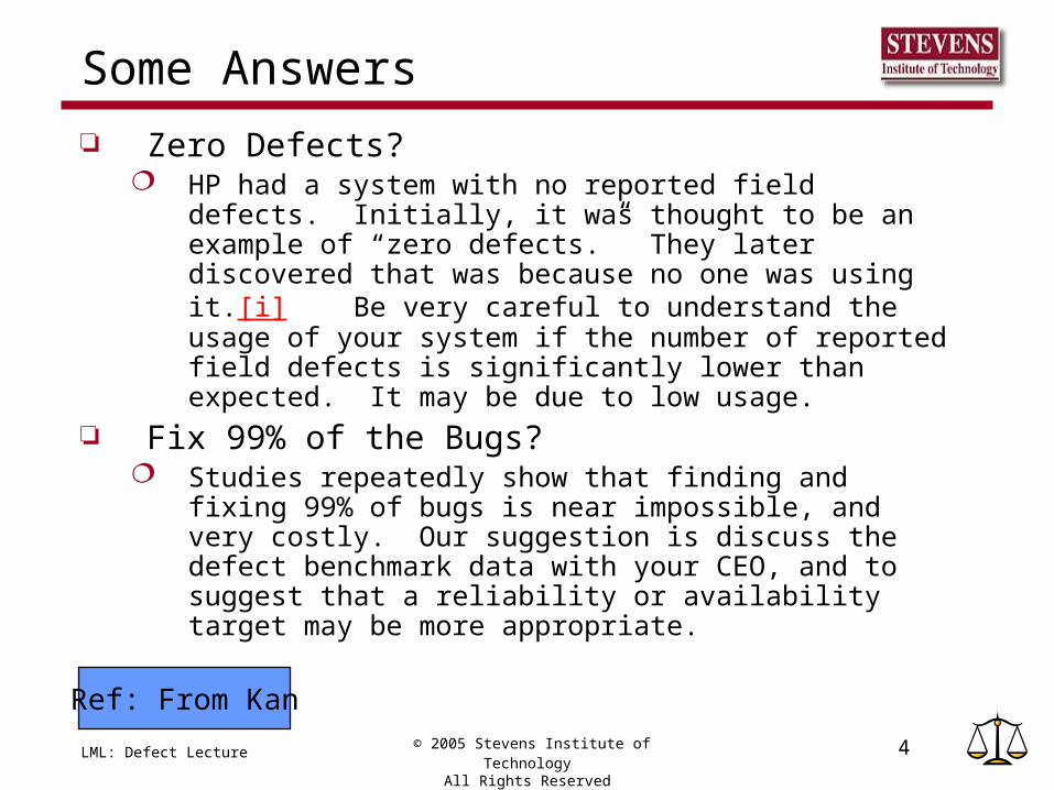
Some Answers

Zero Defects? HP had a system with no reported field defects. Initially, it

was thought to be an example of “zero defects.” They later discovered that was because no one was using it.[i] Be very careful to understand the usage of your system if the number of reported field defects is significantly lower than expected. It may be due to low usage.

Fix 99% of the Bugs? Studies repeatedly show that finding and fixing 99% of

bugs is near impossible, and very costly. Our suggestion is discuss the defect benchmark data with your CEO, and to suggest that a reliability or availability target may be more appropriate.

Ref: From Kan



In Praise of Defects

Are defects good or bad?



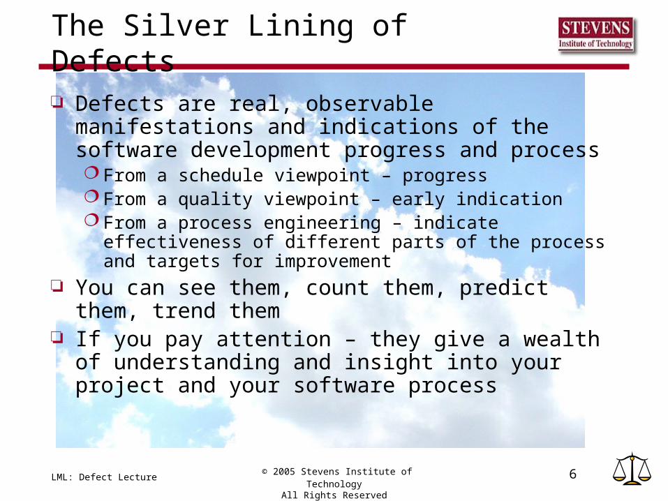
The Silver Lining of Defects

Defects are real, observable manifestations and indications of the software development progress and process From a schedule viewpoint – progress From a quality viewpoint – early indication From a process engineering – indicate effectiveness of

different parts of the process and targets for improvement You can see them, count them, predict them, trend

them If you pay attention – they give a wealth of

understanding and insight into your project and your software process



Defects Table of Contents

Faults and Failures Defect Severity Classification Defect Dynamics and Behaviors Defect Projection Techniques and Models

Dynamic Models Static Models

• Defect Removal Efficiency• Coqualmo

Defect Benchmarks Cost Effectiveness Of Defect Removal Using Defect Data Some Paradoxical Patterns for Defect Data

Key Concept – Make sure you understand Coqualmo Model





Defects and Reliability

A fault leads to a failure.

Defect Metrics are measuring Faults (aka Bugs).

Reliability Metrics are measuring Failures.

People make errors.These are key concepts – REMEMBER THEM – especially the difference between faults and failures



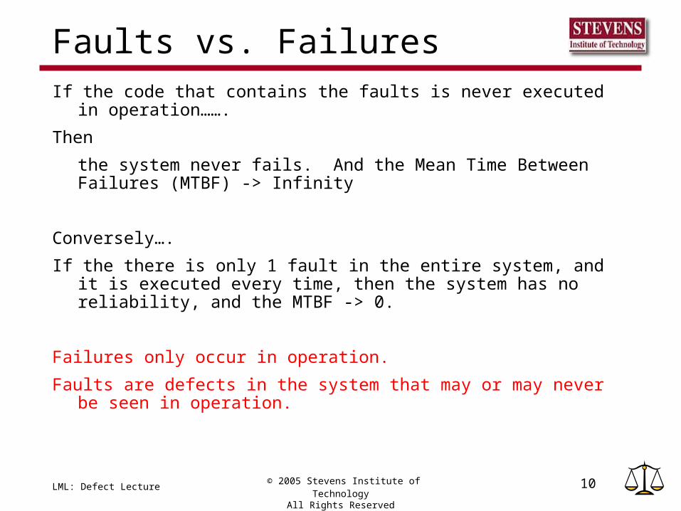
Faults vs. FailuresIf the code that contains the faults is never executed in operation…….

Then

the system never fails. And the Mean Time Between Failures (MTBF) -> Infinity

Conversely….

If the there is only 1 fault in the entire system, and it is executed every time, then the system has no reliability, and the MTBF -> 0.

Failures only occur in operation.

Faults are defects in the system that may or may never be seen in operation.



Measuring Defects

Defect Density: Standard quality measure Number of defects per KLOC or FP

Defect Arrival Rates/Fix Rates: Standard Process and Progress Measurements Defects detected/fixed per unit of time (or effort)

Injected Defects: Defects which are put into the product (due to “errors” which people make) When you have excellent processes, you have fewer

injected defects You can never know completely, how many injected defects

you have in your product – you can only estimate them Removed Defects: Defects which are identified and

then taken out of the product Due to some defect removal activity, such as code reviews



Defect Severity Schemes

Faults can range from crucial to inconsequential

Must have a severity scheme that allows you to differentiate

Severity scheme needs to be based upon the projectWant to focus on defects that will actually

impact your project and product performance



Defect Severity Classes Equivalence class of defects…set of defects which

have ~ the same impact on the project Typically a combination of subjective, indirect metric which

considers both the impact on development progress and to the user if it were to be delivered to the field

Typically critical, major, minor, or some numerical scale More than 5 points is usually unmanageable Most projects tend to use a 4 point scale, and the lowest

priority tends to be rarely fixed When analyzing defect data

Can separate to individual classes Or Use Totals Or Combinations



Defect Dynamics and Behaviors



Defect Dynamics and Behaviors

Defects have certain dynamics, behaviors, and patterns which are important to understand in order to understand the dynamics of software development

This is information that should become part of your “intuition” about software development – your knowledge that this is how software development typically behaves.



Projected Software Defects

In general, follow a Rayleigh Distribution Curve…can predict, based upon project size and past defect densities, the curve, along with the Upper and Lower Control Bounds

Time

Defects

Upper Limit

Lower Limit



Defects vs. Effort

Linear Relationship Between Defects and Effort (e.g, Staff Months)

Defects

Effort

Due to non-linear relationship of effort to productivity

Source: Putnam & Myers



Defects Detected tends to be similar to Staffing Curves – time lag for error dectection

Source: Industrial Strength Software, Putnam & Myers, IEEE, 1997

Time

People

Defects



Which is related to Code Production Rate

And all tend to follow Rayleigh Curves

Note: Period during test is similar to exponential curve

Source: Putnam & Myers

TEST

Code ProductionRate

Time

People

Defects



What conclusions can YOU draw from this?

My view: People tend to make errors (which lead to defects) at a relatively constant rate…..E.G., the more people and the more

effort….the more defects (unless, of course, they are working to prevent or remove defects)



Defect Density vs. Module Complexity

The bathtub chart

Average Component Complexity

Defects per KLOC

Ref: Hatton, Les, “Why don’t we learn from our mistakes?”, 1997

Where do you want to be?



Implications of the Bathtub Curve

Concentrate defect detection on modules that have either very high or very low complexity

Truncate complexity to force fewer defects

Defects perKLOC

Average component complexityRef: Hatton, Les, “Why don’t we learn from our mistakes?”, 1997



Defect Density vs. System Size

Ref: Putnam and Myers, Industrial Strength Software, 1997

10^2 10^3 10^4 10^5 10^6 10^7

10^5

10^4

10^3

10^2

10

1

Defects

Effective Source Lines of Code

Defects found from Integration to Delivery – QSM Data Base



US Industry Ave. for Software Defects

51202560128064032016080402010

1 2 4 8 16 32 64 128 256 512 1024 2048 4096 8192 16384 32768 65536

Below Average

Above Average

Source: Jones, Applied Software Measurement, 1991, Mcgraw-Hill, p 165

Total Potential Defects

App Size in FPs

Basically, the same trend as previous chart



Defect Projection Techniques and Models



Defect Projection Techniques and Models

The objective of defect prediction and estimation techniques and models is to project the total number of defects their distribution over time.

Types of techniques - vary considerably Dynamic models are based upon the statistical distribution

of faults found. Static models use attributes of the project and the process to

estimate the number of faults. Static models can be used extremely early in the

development process, even before the tracking of defects begins.

Dynamic models require defect data from the project, and are used once the tracking of defects starts.



Dynamic Defect Models

Based on predicting, via calculations or tools, the distributions of faults, given some fault data. Primary concept: the defects do follow distribution

patterns, and given some data points, you can generate the arrival distribution equations.

There are many different defect distribution equations Primary ones are Rayleigh, Exponential, and S-

Curves. • Rayleigh distributions are for modeling the entire

development lifecycle• Exponential and S-Curves are applicable for the

testing/deployment processes.



Rayleigh and Exponential Curves

Both in the family of Weibull curves; Which have the form of:

• F(t) = 1 – e(-t/c)m ;• f(t) = (m/t)*(t/c)me (-t/c)m

For m = 1Exponential DistributionFor m = 2 Rayleigh Distribution



Dynamic Distribution Curves

S-Shaped Curve

Exponential

Time

CumulativeFailuresFound Rayleigh Curve

Note-there are infinite Rayleigh, S, and Exponential curves. These just give you a look at the shapes.



Defect Distribution functions

There are 2 primary functions in defect distributionf(t) = Probability distribution function (PDF) of

arrival rates of defectsF(t) = Cumulative distribution function (CDF) of total

number of defects to arrive by time t. They are related by:

F(t) =

And f(t) describes the distribution of the defect arrivals– it can be a uniform distribution, normal, or other distributions

t

dttf0

)(



Rayleigh Model

Defect Arrival Rate (PDF) – the number of defects to arrive during time t =

Cumulative Defects (CDF) -- the total number of defects to arrive by time t =

Where the c parameter is a function of the time tmax that the curve reaches its peak

c = tmax * sqrt (2) K=total number of injected defects

)1(*)(2)/( cteKtF

2)/(2 *)/2(*)( ctectKtf



Plotting the graphs/working with the fxnsF(t) = probability of 1 defect arriving by time t (K=1 – e.g., total number of defects)

f(t) = probability of defect arriving at time 1 (K=1)

What do these charts mean?

Also, if c is supposed to = tmaxmax* sqrt(2), * sqrt(2), does it work?

Raleigh distribution - c=2

-0.2

0

0.2

0.4

0.6

0.8

1

1.2

0 5 10 15

time

pro

ba

bil

ty

F(t) for c = 2

f(t) for c = 2

Raleigh Distribution c = 10

0

0.2

0.4

0.6

0.8

1

0 5 10 15 20

time

pro

ba

bil

ity

F(t) for c = 10

f(t) for c = 10



Plotting the graphs/working with the fxnsThese are all for K = 1.

For case 1, tmax ~ = 1.4, => c = ~ 1.96 (close to 2)

For example, the probability that the defect will arrive at time 2 is ~.39, and the probability that it has arrived by time 2 is ~.62

For case 2, tmax = ~7 => c = 7*1.4 = 9.8 (almost 10)

Raleigh distribution - c=2

-0.2

0

0.2

0.4

0.6

0.8

1

1.2

0 5 10 15

time

pro

ba

bil

ty

F(t) for c = 2

f(t) for c = 2

Raleigh Distribution c = 10

0

0.2

0.4

0.6

0.8

1

0 5 10 15 20

time

pro

ba

bil

ity

F(t) for c = 10

f(t) for c = 10



Predicting defects using data points and the Rayleigh Distribution

This means you can – assuming a Rayleigh Distribution….Mathematically determine the curve and

the equation, as long as you’ve hit the maximum.

Also, the percent of defects that have appeared by tm = 100*F(tm)/K = 100*(1 – exp (-.5)) = 40%. Therefore, ~40% of the defects should appear by time tm.



Methods for using the Rayleigh Distribution

Given n data points, plot them Determine tmax (the time t at which f(t) is max) Then since you have the formulae

Where F(t) is the cumulative arrival rate,f(t) is the arrival rate for defects, and K is the total number of defects…

And you can then use these to predict the later arrival of defects.

2)

2

2)2

2/1(2

2/1(

)/1()(

1)(

tm

tm

tm

t

tetKtf

eKtF



Extremely Simple Method – the 40% rule

Given that you have defect arrival data, and the curve has achieved its maximum at time tm (e.g., the inflection point), you can calculate f(t), assuming the Rayleigh distribution. The simplest method is to use the pattern that ~40% of the total defects have appeared by tm. This is a crude calculation, but is a place to start.



Extremely Easy Method Example

Faults vs. Days

0

20

40

60

80

100

1 2 3 4 5 6 7 8 9

Days

Fa

ult

s F

ou

nd

Tm -> 7

Therefore, expected total number of faults = 429*(100/40) = 1072 or ~1075

Then you can determine f(t), since you know K and Tm

Given the data shown below (429 defects by Tm) – determine f(t) and F(t)



Example continued

Since:

Then substituting in:f(t) = 1075 * t /49 * e- t^2 /98

• = 21.93 * t * e- .01t^2

F(t) = 1075 *[1 - e- .01t ^2] Then you could plot this out on the

same chart and see how well it matches the data.

22

22

)*2/1(2

)*2/1(

)/1()(

1)(

ttm

tt

m

m

tetKtf

eKtF



Predicting Arrival Distributions: Method 2

You can solve for f(t) by using tmax and one or more data points to solve for K and f(t). The simplest way is to take just one data point.



Example: 594 Faults found by day 9

Faults vs. Days

0

20

40

60

80

100

1 2 3 4 5 6 7 8 9

Days

Fa

ult

s F

ou

nd

What is the arrival function f(t)? Need tmax and K to determine f(t).

Tmax -> 7 )2)27*2/1(2)7/1(*)( tteKtf



Then what would you do?

Solve for K (use t = 1, defects = 20) => K=20*49/e(-1/98)= ~990

You now have an equation:

Then plot out the equation and use it to predict arrival rates (and also see how well it matches to data!)

2)98/1()49/990()( ttetf 201.2.20 tte



Statistically Correct?

At least three points are needed to estimate these parameters using non-linear regression analysis, and that further statistical tests (such as Standard Error of Estimate and Proportion of Variance are necessary) for these parameters to be considered statistically valid.

In the case where high precision is important, use a statistical package or one of the reliability tools to calculate the line of best fit.



Statistically Close?

You can use either of the two previous methods… Or as an interim, and easier step, you can calculate K

for all known values of t and f(t), and then take the mean and standard deviation.

That is, K= (49*f(t) * e –.01*(t^2))/t. These calculations are easily performed with a spreadsheet.

Note: these calculations are sensitive to tm although they are not completely valid in a statistical sense,

they give the statistically-challenged practitioner a relatively easy method for calculating the distribution functions, with some initial control limits. Considering the precision of the typical data, this seems reasonable



What do these charts mean?

If the defect data is a reasonable fit for a rayleigh curves…then you can use it to predict outstanding defects, and defect arrival rates



Method 3: Predicting the arrival rates given total number of defects and schedule

Once you predict the total number of defects expected over the life of a project, you can use the Rayleigh curves to predict the number of defects expected during any time period by using the equations below. You can also compare projected defects with actual defects found to determine project performance.

Td is the total duration of the project, such that 95% of all defects have been found.[1] K is the total number of faults expected for the lifetime of the delivery.

Then the defects for each time period t is: f(t) = (6 K/ (Td

2))*t*e ^(-3(t/ Td )2)

[1] The 95% number here is used as a reasonable target for delivery. The equations are derived from F(Td)/K = .95 Another percentage would result in slightly different constants in the equations.



Example: Method 3

Assume that:similar projects have had a defect density of 10.53

defects per 1KLOCthe predicted size is 100KLOC. you expect to have 5% fewer defects (process

improvements!).therefore, you project that the total number of

defects for this project will = 10.53*100*.95 = 1000.

ThenSince f(t) = (6 K/ (Td

2))*t*e ^(-3(t/ Td )^2)And given Td=26 weeksThen

• f(t) = 6000/676 * t * e ^ (-3/676* (t^2))• f(t) = 8.76 * t * e ^ (-.00444*t^2)



Example Continued - Graphically The expected distribution of faults would be:

Based upon the distributions in your data from prior projects, you can add in control limits. You may want to use 2SD which will give you a 95% confidence range of performance.

If you do not have data from prior projects, you can still project overall defect densities in a number of ways, as discussed later in this lecture, and use the same technique to project arrival rates.

Defects Per Week

0

10

20

30

40

50

60

0 10 20 30

Week

Defe

cts

Fo

un

d



Why would you want to predict defect arrival patterns from the schedule?

To allow you to compare what is actually occurring, to what you predict will happen



Tools

The Rayleigh model is used in a number of tools. Some of the more notable ones are:SPSS (Regression Module)SAS (by SAS)SLIM (by Quantitative Software

Management)STEER (by IBM).



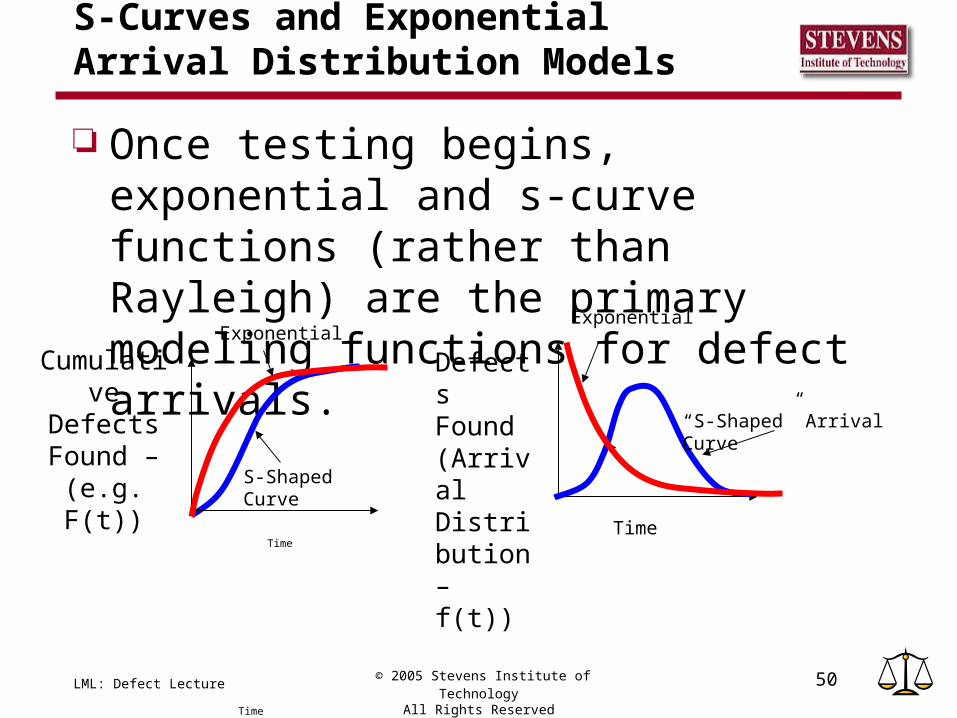
S-Curves and Exponential Arrival Distribution Models

Once testing begins, exponential and s-curve functions (rather than Rayleigh) are the primary modeling functions for defect arrivals.

“S-Shaped” Arrival Curve

Exponential

Time

DefectsFound(Arrival Distribution – f(t))

Time

S-Shaped Curve

Time

CumulativeDefectsFound –

(e.g.F(t))

Exponential



S-curves

Resemble a S a slow start a much quicker discovery rate a slow tail-off at the end

Based on the concept initial defects may be more difficult to find because of either

the length of time for error isolation, or due to crucial defects which need to be fixed before others can be found

Multiple S-curve models; all are based upon the non-homogeneous Poisson process for the arrival distribution. One equation for S-curves is:

F(t) = tetK )1(1



Exponential Distributions

F(t) = K*(1 – e-λt) f(t) = K*(λ t* e-λt )

Exponential

Time

CumulativeFailuresFound

K – total number of defects



Using exponential curves

Given a set of data points, you want to know K. The techniques are similar to those for Rayleigh curves. You can:

Use Reliability/Statistical Analysis Tools Solve for a few points (Eyeball in your own K…but don’t tell

anyone I said that).



Some of my students have suggested that these patterns sound like a lot of ….



Let us look at some results….



Empirical Data for the Rayleigh Models - 1

Putnam and Myers (1992) - total defects projected using Rayleigh curves within 5% to 10%. (!!)Others were not as close, but the data may have

been dirtier. Biswas and Thangarajan (2000) from Tata Elxsi

Ltd reported on using a Rayleigh model successfully on over 20 projects

IBM Federal Systems in Gaithersburg, MD using their STEER software tool estimated latent defects for 8 projects and compared the estimate with actual data collected for the first year in the field. The results were “very close.”

Ref: Thangarajan & Biswas,

“Mathematical Model for Defect Prediction across Software Development Lifecycle”

Ref: Hollenback, “Quantitatively Measured ProcessImprovements at Northrop Grumman IT,” 2001



Rayleigh Results -2

Below are charts from Northop Grumman [ii] in 2001, which show their successful use of the Rayleigh Model to predict test defects from defects found earlier in the development cycle.

0

100

200

300

400

500

600

700

800

900

0 1 2 3 4 5 6 7 8 9 10 11 12 13 14 15 16 17 18 19 20 21 22 23 24 25 26 27 28 29 30 31 32 33 34 35 36 37 38

Project Month

Def

ects

Dis

cove

red

Theoretical Curve Actual Values

Defect Discovery Rayleigh CurveAll Test Defects

Feb 03 Prediction = 14.55 defects

Feb 03 Actual = 15 defects

.14 defects per K LOC/month

0

100

200

300

400

500

600

700

800

900

0 10 20 30

Project Month

Def

ects

Dis

cove

red

Theoretical Curve Actual Values

Prediction = 1.44 defects

Actual = 1 defect (last week of May)

Defect Discovery Rayleigh CurveBuild .75 Test Defects



Results - 3….

With small projects, there are fewer data points, and therefore, less confidence.

Some suggest Weibull curves with m=1.8 as the best fit, but the manual calculations become more difficult



Results - 4

Over the past 15 years, and with the move to higher SEI levels, much more defect data has been recorded than ever before.

Even so, organizations will vary from the standard patterns. Defect arrival rates do tend to follow the Rayleigh curves, and the equations can be finely tuned to match an individual environment.



Recommendations for Dynamic Models

Start tracking and using your defect data if you are not doing it.

Use as many models as possible, compare them with each other, track the results, and see what works best for you.



Break Time - Get some Caffeine!



Now let us shift gears from Dynamic Models to Static

Models



Static Defect Models

Based upon software development process and past history – not defect data for this projectCan use extremely early in the dev

processUseful for evaluating and predicting the

impact of process changes on quality



Fundamental Defect Model

The most useful model I’ve seen for dealing with defects is one developed by Boehm and Jones….

It basically says that given a software project – you have defects being “injected” into it (from a variety of sources) and defects being removed from it (by a variety of means)

Good high-level model to use to guide our thinking and reasoning about defects and defect processes



Defect Introduction and Removal Model – Boehm

and Jones

Inspections

Reviews

PrototypingTesting

Defects Injected

Defects removed

RqmtsCodingDesign

The Product



Defect Model Continued

So, based on this model, the goal in software development, for delivering the fewest defects, is to:Minimize the number of defects that go inMaximize the number of defects that are

removed

The obviously is actually good --- it means the model matches our intuition



Defect Removal EfficiencyA key metric for measuring and

benchmarking the process by measuring the percentage of possible defects removed from the product at any point in time



Defect Removal Efficiency

Both a project and process metric – can measure effectiveness of Quality activities or the quality of a project

DRE = E/(E+D) Where E is the number of errors found before delivery to the end

user, and D is the number of errors found after delivery. The Goal is to have DRE approach 1

Or DREi = Ei / (Ei + Ei+1) Where Ei is the number of errors found in a software engineering

activity i, and Ei+1 is the number of errors that were traceable to errors that were not discovered in software engineering activity I.

The goal is to have this approach 1 as well…e.g., errors are filtered out before they reach the next activity

Source: Software Engineering, Pressman, 200, McGraw-Hill



DRE Examples:

You found 10 defects after you delivered your product. There were 990 defects found and removed before delivery. Your DRE = 990/1000 = 99%.

You found 10 requirements defects when you were in coding and testing. Luckily, you found none after that, and you hope you got them all. During your requirements process, you found 40 requirements defects. What is your DRE for the requirements process? 40/50 = 80%.



Using the DRE as a Static Model

Projects that use the same team and the same development processes can reasonably expect that the DRE from one project to the next are similar.

For example, if on the previous project, you removed 80% of the possible requirements defects using inspections, then you can expect to remove ~80% on the next project.

Or if you know that your historical data shows that you typically remove 90% before shipment, and for this project, you’ve used the same process, met the same kind of release criteria, and have found 400 defects so far, then there probably are ~50 defects that you will find after you release.



Defect Removal Matrix

Matrix which identifies both where defect was found as well as insertedThe more steps in your process, the bigger

the matrix

Useful as an analysis tool for process Allows calculation of efficiencies of test

removal for each step in process.

Kan



DRE Matrix Example:

Defect Removal Step

Rqmts

Design

Coding

Rqmts Review 5 5Design Review 8 10 18Testing 3 17 25 45

16 27 25

Given matrix at right

1. The number of total defects removed in the design review =

2. Defects injected in coding phase =

3. Defect Removal of each step

1. Rqmts Review =

2. Design Review =

3. Testing=

Lets try doing this



DRE Matrix Example

Defect Removal Step

Rqmts

Design

Coding

Rqmts Review 5 5Design Review 8 10 18Testing 3 17 25 45

16 27 25

Given matrix at right

1. The number of total defects removed in the design review = 18

2. Defects injected in coding phase = 25

3. Defect Removal Efficiency of each step

1. Rqmts Review = 5/16 = 31%

2. Design Review = 18/11+27=18/38=47%

3. Testing=45/20+25=100%



Using the DRE Matrix

What does this Matrix tell you? If it were your project, what would you do?

First, I’d extend it to have customer reported data (this is just a short coming of this example)

Next, with the data we have, I’d Focus on improving the design review process. Typical

rules of thumb for design reviews are 60% to 70% removal vs. the 47% we have here.

Determine why there are so many design review defects. This seems like a high number vs. the amount of effort usually spent in this phase. Perhaps more prototyping is needed.



Variety of static defect model tools available, some commercially, some freeware

Tools allow tuning for your environment Will look at one tool, COQUALMO,

which was a research project and an extension to COCOMO-II.

Static Defect Model Tools



COQUALMO – by Chulani and Boehm Defect Analysis Tool from USC Extension to the COCOMO estimation model (Software

Sizing Model developed by Boehm and others at USC) Current data is from the COCOMO clients and “Expert

Opinion” Need add’l data from more projects to tune the model Based on the Defect Insertion/Removal model Tool available on our course website



Coqualmo is a model which predicts…Delivered

Defect Density (per KLOC or per FP)

Inspections

Reviews

PrototypingTesting

Defects In

Defects out

RqmtsCodingDesign

The Product

Based upon a variety of factors…And which you can tune based on your own experience.

Delivered Defect Density



Coqualmo Models

2 Separate models

Source: COCOMO II

Size

Software Platform, Product, Personnel, and Project Attributes

Defect Introduction

Number of non-trivial reqmts, design, and coding defects introduced

Defect Removal

Number of Defects per KLOC

Defect Removal Activities (Automated Analysis, Reviews, Testing and Tools)



Defect Introduced (DI) Defined

Defects Introduced (DI) = the sum of the number of defects introduced in the requirements, design, and coding phases

The number of defects introduced in a given phase = A * (size) B * QAF where A is a multiplicative constant based upon the phase B is based upon size (in KLOC) and accounts for economies

of scale QAF is based upon the quality of the process, platform, etc.

Algebraically, DI = Initially, A = 10 for requirements, 20 for design, 30 for code B is initially set to 1 QAF is the quality adjustment factor that is taking into

account 21 defect introduction drivers (Platform, Product, Personnel, and Project) from COCOMO

jB

jj QAFSizeA j **

3

1



Example (Using dummy data):

Assume that you calculated the QAF for each phase --- and that you have the following values, and that the model has given you the values for A as shown

This says that the Defects Introduced by phase would be:

Phase QAF ARqmts 1.2 10Design 1 20Coding 0.5 30

Phase QAF A DIRqmts 1.2 10 12Design 1 20 20Coding 0.5 30 15

Note that the QAFs imply a requirements activity worse than average and a coding activity better than average



Example continued

If your product had 5K of code, and you used B=1, then you would project:

So you project that a total of 235 defects will be injected into the product

Phase DI DefectsRqmts 12 60Design 20 100Coding 15 75



Defects Introduced

Nominal values, per KSLOC are: DI(requirements) = 10; DI (design) = 20 DI (coding) = 30 DI(total) = 60

E.G., for for every 1K lines of code, the model predicts that, assuming a “nominal situation” there would typically be 60 defects injected into the code, 10 of which were requirements defects, 20 were coding, etc. etc.

For the QAF, the Process Maturity factor had highest impact on defect introduction with everything else held constant, it varies result by a factor of

2.5…which says that if you have a very good process, you significantly reduce the number of defects introduced



Now lets look at defects removed

Inspections

Reviews

PrototypingTesting

Defects Injected

Defects removed

RqmtsCodingDesign

The Product

Delivered Defect Density



COQUALMO – Defect Removal

Initial values determined by experts using the Delphi techniques

Looked at three different removal techniques: Automated Analysis, People Reviews, Execution Testing and Tools

Rated %DRE for 6 levels of effectiveness of technique for each phase (rqmts, design, coding)

For example, I computed residual defects as If all techniques “Very Low Effectiveness” = 60 defects

per KSLOC If all techniques “Extra High Effectiveness” = 1.57 defects

per KSLOC If all techniques “Nominal” = 14.3 defects per KSLOC



Summary on COQUALMO model

Mathematical model which takes as input Your view of your defect injection driversYour view of your defect removal drivers

Gives you a projection of # of defects remaining in your system

Can be used to estimate impact of “driver changes” on defect density“what if” analysis“improvement investment” analysis



LML Commentary

I think the COQUALMO model gives superb base line information, which an organization can use to engineer and the tune is defect prevention, injection, and removal processes.



Now let us shift gears from Defect Benchmark Data



Defect Benchmark Data

Data is surprisingly sparse. Many companies hold it very proprietary. Easy to misuse the data,

punishing projects that somehow are not meeting certain benchmarks

misleading results caused by differences in counting techniques, such as in size, usage, and severity.

Don Reifer[i] has taken a lead in publishing software productivity, cost, and quality data, in hopes of encouraging others to do so.

[i] Reifer, Don, The DoD Software Tech News, “Software Cost, Quality, & Productivity Benchmarks”, July 2004



Defect Data By Application Domain - Reifer

Application Domain Number Projects

Error Range (Errors/

KESLOC)

Normative Error Rate Notes

(Errors/ KESLOC)

Automation 55 2 to 8 5 Factory automation

Banking 30 3 to 10 6 Loan processing, ATM

Command & Control 45 0.5 to 5 1 Command centers

Data Processing 35 2 to 14 8 DB-intensive systems

Environment/ Tools 75 5 to 12 8 CASE, compilers, etc.

Military -All 125 0.2 to 3 < 1.0 See subcategories

Airborne 40 0.2 to 1.3 0.5 Embedded sensors

Ground 52 0.5 to 4 0.8 Combat center

Missile 15 0.3 to 1.5 0.5 GNC system

Space 18 0.2 to 0.8 0.4 Attitude control system

Scientific 35 0.9 to 5 2 Seismic processing

Telecom 50 3 to 12 6 Digital switches

Test 35 3 to 15 7 Test equipment, devices

Trainers/ Simulations 25 2 to 11 6 Virtual reality simulator

Web Business 65 4 to 18 11 Client/server sites

Other 25 2 to 15 7 All others



Reading the Previous Chart

Reifers data is Delivered Defects per KLOC.



Domain Data Comments

Defect rates in military systems are much smaller due to the safety requirements

Defect rates after delivery tend to be cyclical with each version released. They initially are high, and then stabilize around 1 to 2 defects per KLOC in systems with longer lifecycles (> 5 years). Web Business systems tend to have shorter lifecycles (<=2 years) and may never hit the stabilization point.



Cumulative Defect Removal (Reviews, Inspection,Testing)

1024051202560128064032016080402010

60% 65% 70% 75% 80% 85% 90% 95%

Source: Jones, 1991

App Size in FPs

Below Average

Above AverageWhat does this imply?



Industry data – SEI Levels

CMM Approach

Measure Average defects/ function points

Typical defect potential and delivered defects for SEI CMM Level 1

5.0 Injected.75 delivered









Source: Capers Jones, 1995



Industry Data

Industry Approach

Measure Average defects/ function points

Delivered defects per industry System Software - .4Commercial Software - .5Information Software - 1.2Military Software - .3Overall average - .65

Source: Capers Jones, 1995



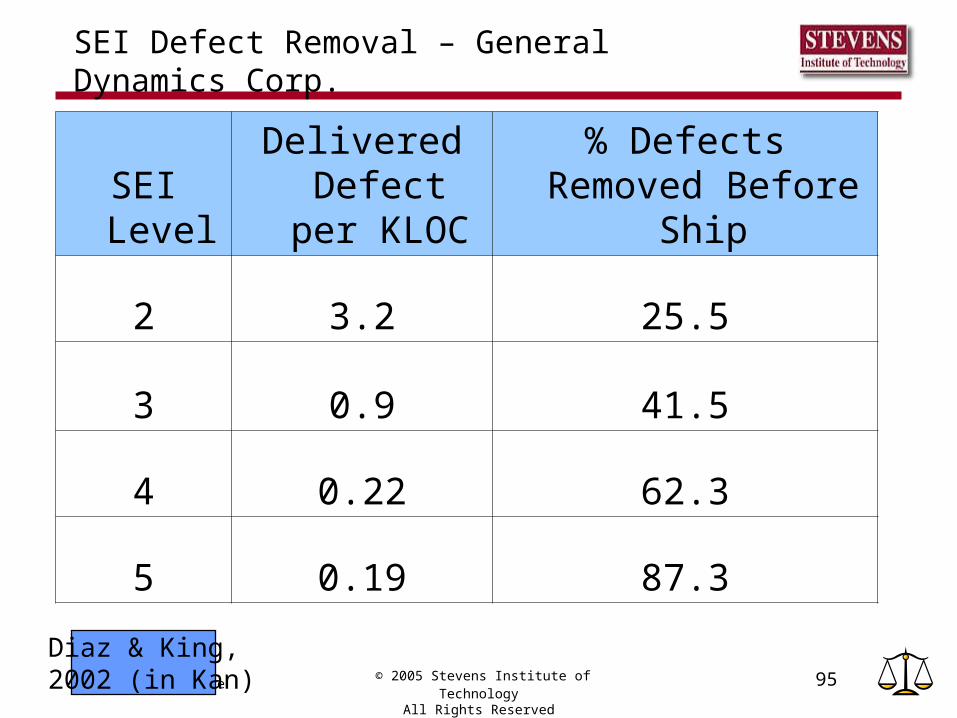
SEI Defect Removal – General Dynamics Corp.

Diaz & King, 2002 (in Kan)

SEI Level

Delivered Defect per

KLOC% Defects Removed

Before Ship

2 3.2 25.5

3 0.9 41.5

4 0.22 62.3

5 0.19 87.3



Pop Quiz: Good or bad quality

You estimate that your delivered defect rate is 2 per KLOC. You have a military application. Is this good or bad quality?

Bad….for military



Latent Defects

Two different studies on millions of lines of debugged and released C and Fortran code by Hatton and Roberts using only static code analyzers found ~6 defects per KLOC. These were faults such as uninitialized variables. Obviously, there are more latent defects in the code than the static analyzers found.

Ref Hatton & Roberts, from Fenton and Pflegger



Cost Effectiveness of Defect Removal by Phase

The later defects are removed, the more expensive they are to remove.

IBM data – Remus (1983)Cost Removal Ratios

• Design/Code Inspection – 1x• Testing – 20x• Customer use – 82X

Other Data/Benchmarks – 5 to 10x more for each phase



Defect Removal Patterns

0

5

10

15

20

25

30

I0 I1 I2 UT CT ST

Development Phase

De

fec

ts/K

LO

C

Prod 1

Prod 2

Which do you prefer?



Defects found earlier cost less to fix

Therefore, prefer the red columns rather than the blue ones.

Lets calculate the difference in cost – see what the difference is?What are typical rates of costs of bug fixing in design vs. code

vs. test (internal)?Use 1:20:85What is your estimate of % difference in cost for this case?

If we assume $100 for a fix in designTherefore, $2000 for each fix in coding, and $8500 for each fix in

testing



Cost to Find/Fix Defects by Phase

If we use the find/fix cost ratio to be 1:20:85 for Design:code:test, then what is the ratio of the cost for product 1 vs. product 2 is 1590/953 = ~1.6 which is ~70% more … or $160K vs $95K

Cum Cost

0

500

1000

1500

2000

I0 I1 I2 UT CT ST

Phase

$$ i

n 1

00s

(Ass

um

ing

100

to

fix

a d

esi

gn

bu

g)

Cum P1

Cum P2



Engineering Rules for Cost Of Defect Removal

Ratios will be based upon your situation. Do you have one field site or 200? Can patches be downloaded easily, or is a site visit required,

along with database upgrades? Do you have extensive integration and regression testing?

We recommend that you gather your own data and understand the costs for your own environment.

Short of using your own data, we recommend using the following multiplicative factors: Cost for fixing in Requirements/Design – 1X Cost of fixing in Coding Phase – 5X Cost of fixing in Formal Testing Phase – 5X Cost of fixing in Field – 5X.



Using Defect DataMeasurement Constructs Model Examples of Usage



Using Defect Data

Most projects track defect dataVery important quality data

Can be used in a variety of ways – 2 are:Data to project mgmt while development

underway to allow active mgmt based on real information

Data to process engineers to improve the development process



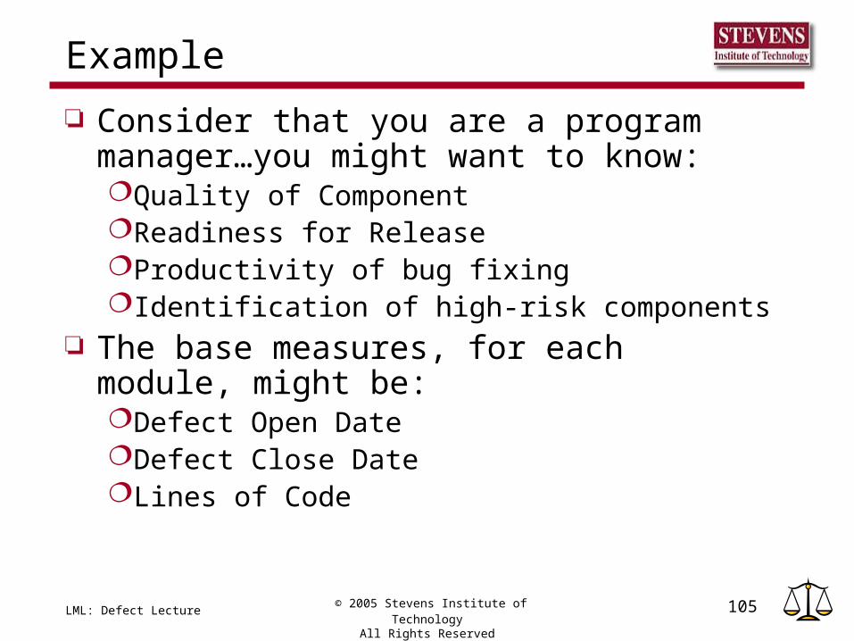
Example

Consider that you are a program manager…you might want to know:Quality of ComponentReadiness for ReleaseProductivity of bug fixingIdentification of high-risk components

The base measures, for each module, might be:Defect Open DateDefect Close DateLines of Code



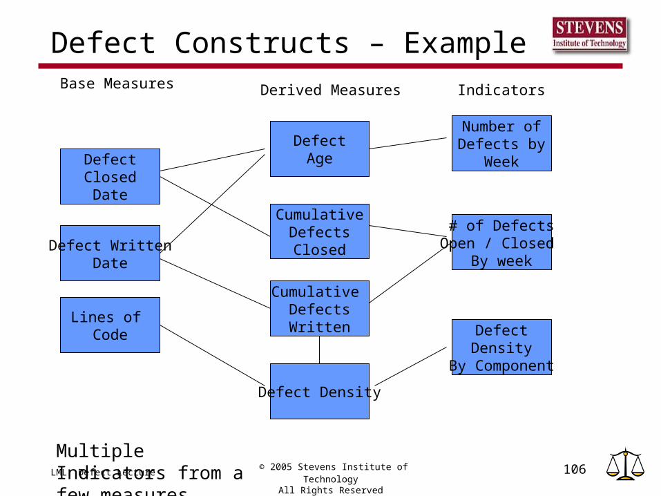
Defect Constructs – Example

DefectClosedDate

Defect WrittenDate

Lines of Code

Defect Density

Cumulative DefectsWritten

CumulativeDefectsClosed

DefectAge

Defect Density

By Component

# of DefectsOpen / Closed

By week

Number ofDefects by

Week

Base Measures Derived Measures Indicators

Multiple Indicators from a few measures



Defect Aging Indicator

Defect Aging

0

20

40

60

80

100

1 2 3 4 5 6 7 8 >=9

Weeks Open

Number of Defects Open

Defect Age Limit

Are defects being closed out “on time?” Why do we have “old defects”? Especially >=9 weeks? What are they?



Open/Closed Defect Indicator

Open/Closed Defects

0

10

20

30

40

50

60

70

1 2 3 4 5 6 7 8 9 10

Weeks

# o

f D

efe

cts

Written

Closed

When can we release this product? How good will it be?



Open/Closed Defect Indicator –1

Defect Status

0

50

100

150

200

250

300

1 2 3 4 5 6 7 8 9

Week

Num

ber

of D

efec

ts

Cum Written

Cum Closed

Open per Week

When will the release be ready to ship? How are we progressing?



Some Commentary

Many things are going on in these projects – these are indicator metrics which help the project manager understand what is going on

Need to also look at other data such as testing progress



Defects/KLOC

0

0.01

0.02

0.03

0.04

0.05

0.06

0.07

0.08

1 2 3 4 5

Releases

Def

ects

/KLO

C

Defects/KLOC

Defect Density by Release (or Module)

Target Range: .022 to .058(Historical)

What’s the Quality of Release?Have we done adequate testing on 3 and 5?



Open Defects – Another Example

Status of Defects

01020304050607080

1 2 3 4 5 6 7 8 9 10 11 12

Weeks

Nu

mb

er

of

De

fect

s

Open

New

Closed

What does this tell you?



What Does this chart Tell you?

Macro: Quality: Looks Like the release is improving Need to in more detail (trends) at new vs. closed Appears that team can fix ~10 defects per week When will we be ready to release?

Status of Defects

01020304050607080

1 2 3 4 5 6 7 8 9 10 11 12

Weeks

Nu

mb

er

of

De

fects

Open

New

Closed



Analysis of New vs. Closed

New vs. Closed Defects

0

5

10

15

20

25

1 2 3 4 5 6 7 8 9 10 11 12

Weeks

# o

f D

efe

cts

New

Closed

For Closed Defects, Mean = 12.3, STD = 2.3 Implications: Appears to be an upper limit on number defects can be closed in a week – and can look at a view of optimistically 15, pessimistically 10.For New Defects, appears to be trending lower. Implications….looks like 3 to 5 more weeks until ~ 1 or ~2. Also, if you can “explain” what happened week 4 and 7, may be different curve….



Summary on Defect Constructs

Can use a few base measures to drive a variety of constructs and indicators, which can be very useful in pointing out potential problem areas, and giving “indicators” of what is really going on.

You can design your own constructs to match the information needs of your organization

Need to then analyze the data, use it to supplement historical data, and to make decisions.

Extremely useful in managing a project quantitatively with “eyes open” rather than qualitatively (“Well, I think everything is going ok”)

Defects are real, observable events…as opposed to opinions and hand waving. They are good data. PAY ATTENTION TO THEM, AND USE THEM TO KNOW WHAT IS GOING ON.



Some Paradoxical Patterns for Customer Reported Defects

Capers Jones pointed out in 1991[i] that there are two general rules for customer reported defects. The number of defects found correlates directly with the

number of users The number of defects found correlates inversely with the

number of defects that exist These general rules seem, at first, to be at odds with

each other, but actually, they are inter-related. They are both based upon the concept that the more the

software is used, the more defects that will be discovered and found.

If the software has many users, it will have more execution time, and hence, more defects will be uncovered.

Conversely, if the software is buggy, people will not use less, and fewer defects will be uncovered.

[i] C. Jones, Applied Software Measurement



Homework



Class problem 2.

Consider the nominal values for defect insertions and removal from the COQUALMO model. (See table 5 of article)If you prevented 40% more defects in the

requirements phase, for a 20 KSLOC system, how many defects would you prevent?



Problem 2, answers.

Consider the nominal values for defect insertions and removal from the COQUALMO model. If you prevented 40% more defects in the requirements

phase, for a 20 KSLOC system, how many defects would you prevent?

For a 20 KSLOC “nominal” system, have approximately 20*10 = 200 defects injected. With the nominal removal, there would be 3.2*20 = 64 (from table 5).

Based on table 5, if we add another 40% step to the bug removal activities for the nominal case, we have the removals of 10%, 40%, 40%, and 40%, which results in .9*.6*.6*.6 = .19 = 19% of the requirements bugs left. Therefore, since we had 200 originally, we have 38 left, so we removed an add’l 64-38=26 bugs.



Readings

Read Coqualmo Article Read Defects Chapter



Project You are now in system test. . For Theater Tickets, you have

the defect arrival data points below. Assume a Raleigh curve What do you predict as the total number of bugs in the system? -

Use two methods.. How many bugs do you predict as being left in the system? What is the equation that predicts the defects? If you shipped at the end of week 6 (and assuming you removed all

the defects found at that time), what would you predict as the defect removal efficiency?

If this is a 5,000 LOC program, what would you predict as the remaining defect density after 6 Months?

Should you ship after 6 Months? Why or why not?

Month Found 1 2 3 4 5 6 Defects 13 22 25 22 17 5



Project Continued

Instead of the data on the previous page, use Coqualmo to predict the number of defects inserted and removed by phase. Assume a “good” development process, and a relatively poor testing process – and use that information to select the values for the factors.

1 LML: Defect Lecture © 2005 Stevens Institute of Technology All Rights Reserved Software Engineering Metrics Linda M. Laird “In Praise of Defects” Stevens.

Documents

defect lecture

software process slide

defect benchmark data

process mfrom

software system

process engineering

answers ozero defects

kan slide