1 Les règles générales WWOSC 2014 16-21 August, Montréal, Canada Didier Ricard 1 , Sylvie Malardel 2 , Yann Seity 1 Julien Léger 1 , Mirela Pietrisi 1. CNRM-GAME, METEO-France, Toulouse 2. ECMWF, Reading Sensitivity of short-range forecasting with the AROME model to a modified semi- Lagrangian scheme and high resolution.

1 Les règles générales WWOSC 2014 16-21 August, Montréal, Canada Didier Ricard 1, Sylvie Malardel 2, Yann Seity 1 Julien Léger 1, Mirela Pietrisi 1. CNRM-GAME,
Dec 14, 2015
Welcome message from author
This document is posted to help you gain knowledge. Please leave a comment to let me know what you think about it! Share it to your friends and learn new things together.
Transcript
1
Les règles générales
WWOSC 2014
16-21 August, Montréal, Canada
Didier Ricard1, Sylvie Malardel2, Yann Seity1
Julien Léger1, Mirela Pietrisi
1. CNRM-GAME, METEO-France, Toulouse
2. ECMWF, Reading
Sensitivity of short-range forecasting with the AROME model to a modified semi-Lagrangian scheme and high resolution.

2
AROME (Seity et al., 2011): operational fine-scale NWP model used at METEO-France since 2008 In 2008: 2.5-km horizontal resolution, 41 vertical levels
Domain 1500 km * 1300 km (600*512 points)
Current version: 2.5-km horizontal resolution, 60 vertical levels
Domain 1875 km * 1800 km (750*720 pts)
In 2015: 1.3-km horizontal resolution, 90 vertical levels
Domain 1996 km * 1872 km (1536*1440 pts)
1 – Introduction
Next version: 1.3 km 90

3
Dynamics package:• Nonhydrostatic model based on a fully compressible system• Spectral model, A grid • Semi-Lagrangian scheme
Tri-linear interpolation for computation of trajectories (origin point) quasi-cubic interpolations for calculating advected variables at origin point
• Time scheme 2 Time Levels semi-implicit scheme with SETTLS option (operational version) ICI (iterative centred implicit) scheme (Predictor-corrector scheme)
• 4th order spectral diffusion and gridpoint SLHD on hydrometeors
Characteristics of the AROME model
Physics package:• one moment mixed-phase microphysical scheme: 5 hydrometeor classes • 1D Turbulence scheme: pronostic TKE equation with a diagnostic mixing length (Bougeault
Lacarrere, 1989)• Surface scheme: SURFEX (ISBA parametrisation, TEB scheme for urban tiles, ECUME for sea tiles)• Radiation scheme: ECMWF parameterization• EDMF Shallow convection scheme
1 – Introduction
4
Evaluation of the AROME model at convective scale for preparing the next operational version
Test of a modified SL scheme at 2.5-km horizontal grid spacing during several periods (in particular between 15 July - 15 September 2013)
Comparison between AROME forecasts at 1.3-km and 2.5-km horizontal resolutions during June-November 2012 for days with thunderstorms
1 – Introduction
5
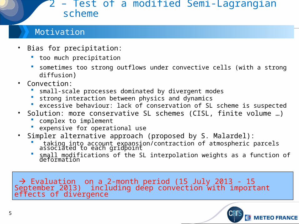
Motivation
Evaluation on a 2-month period (15 July 2013 - 15 September 2013) including deep convection with important effects of divergence
• Bias for precipitation: too much precipitation
sometimes too strong outflows under convective cells (with a strong diffusion)• Convection:
small-scale processes dominated by divergent modes strong interaction between physics and dynamics excessive behaviour: lack of conservation of SL scheme is suspected
• Solution: more conservative SL schemes (CISL, finite volume …) complex to implement expensive for operational use
• Simpler alternative approach (proposed by S. Malardel): taking into account expansion/contraction of atmospheric parcels associated to each gridpoint small modifications of the SL interpolation weights as a function of deformation
2 – Test of a modified Semi-Lagrangian scheme
6
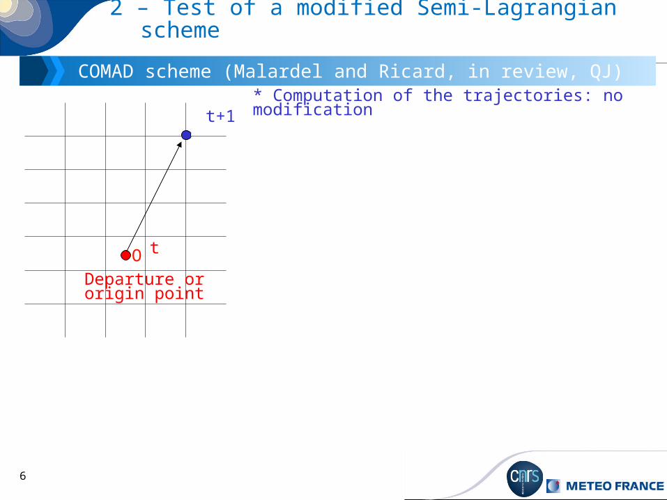
COMAD scheme (Malardel and Ricard, in review, QJ)
2 – Test of a modified Semi-Lagrangian scheme
t+1
Departure or origin point
t
* Computation of the trajectories: no modification
O

7
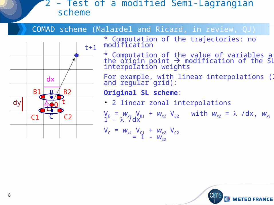
COMAD scheme (Malardel and Ricard, in review, QJ)
2 – Test of a modified Semi-Lagrangian scheme
t+1
t
dx
L
* Computation of the trajectories: no modification
* Computation of the value of variables at the origin point modification of the SL interpolation weights
For example, with linear interpolations (2D and regular grid):
Original SL scheme:
• 2 linear zonal interpolations
VB = wx1 VB1 + wx2 VB2 with wx2 = /dx, wx1 = 1 - /dx
VC = wx1 VC1 + wx2 VC2 = 1 - wx2
dy
B1 B2
C2C1
O
8
COMAD scheme (Malardel and Ricard, in review, QJ)
2 – Test of a modified Semi-Lagrangian scheme
t+1
t
dx
L
* Computation of the trajectories: no modification
* Computation of the value of variables at the origin point modification of the SL interpolation weights
For example, with linear interpolations (2D and regular grid):
Original SL scheme:
• 2 linear zonal interpolations
VB = wx1 VB1 + wx2 VB2 with wx2 = /dx, wx1 = 1 - /dx
VC = wx1 VC1 + wx2 VC2 = 1 - wx2
dy
B1 B2
C2C1
OB
C

9
COMAD scheme (Malardel and Ricard, in review, QJ)
2 – Test of a modified Semi-Lagrangian scheme
t+1
t
dx
L
* Computation of the trajectories: no modification
* Computation of the value of variables at the origin point modification of the SL interpolation weights
For example, with linear interpolations (2D and regular grid):
Original SL scheme:
• 2 linear zonal interpolations
VB = wx1 VB1 + wx2 VB2 with wx2 = /dx, wx1 = 1 - /dx
VC = wx1 VC1 + wx2 VC2 = 1 - wx2
• 1 meridian linear interpolation
VO = wy1 VB + wy2 VC with wy1 = L / dy, wy2 = 1 - L /dy
dy
B1 B2
C2C1
OB
C
10
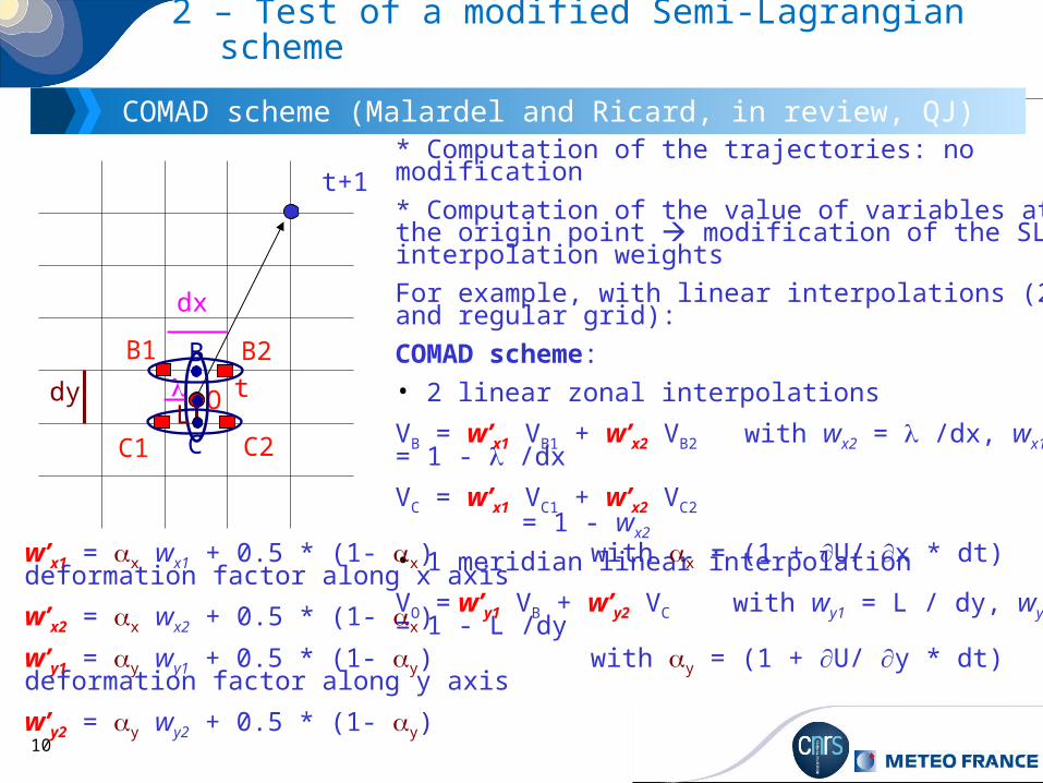
COMAD scheme (Malardel and Ricard, in review, QJ)
2 – Test of a modified Semi-Lagrangian scheme
t+1
t
dx
* Computation of the trajectories: no modification
* Computation of the value of variables at the origin point modification of the SL interpolation weights
For example, with linear interpolations (2D and regular grid):
COMAD scheme:
• 2 linear zonal interpolations
VB = w’x1 VB1 + w’x2 VB2 with wx2 = /dx, wx1 = 1 - /dx
VC = w’x1 VC1 + w’x2 VC2 = 1 - wx2
• 1 meridian linear interpolation
VO = w’y1 VB + w’y2 VC with wy1 = L / dy, wy2 = 1 - L /dy
dy
B1 B2
C2C1
O
B
C
w’x1 = x wx1 + 0.5 * (1- x) with x = (1 + U/ x * dt) deformation factor along x axis
w’x2 = x wx2 + 0.5 * (1- x)
w’y1 = y wy1 + 0.5 * (1- y) with y = (1 + U/ y * dt) deformation factor along y axis
w’y2 = y wy2 + 0.5 * (1- y)
L

11
COMAD scheme (Malardel and Ricard, in review, QJ)
2 – Test of a modified Semi-Lagrangian scheme
t+1
t
B1 B2
C2C1
O
w’x1 = x wx1 + 0.5 * (1- x) with x = (1 + U/ x * dt) deformation factor along x axis
w’x2 = x wx2 + 0.5 * (1- x)
w’y1 = y wy1 + 0.5 * (1- y) with y = (1 + U/ y * dt) deformation factor along y axis
w’y2 = y wy2 + 0.5 * (1- y)
modified linear weights can also be used after for computing cubic weights
B0 B3
C3C0
A1 A2
D1 D2
* Computation of the trajectories: no modification
* Computation of the value of variables at the origin point modification of the SL interpolation weights
For example, with linear interpolations (2D and regular grid):
COMAD scheme:
• 2 linear zonal interpolations
VB = w’x1 VB1 + w’x2 VB2 with wx2 = /dx, wx1 = 1 - /dx
VC = w’x1 VC1 + w’x2 VC2 = 1 - wx2
• 1 meridian linear interpolation
VO = w’y1 VB + w’y2 VC with wy1 = L / dy, wy2 = 1 - L /dy
12
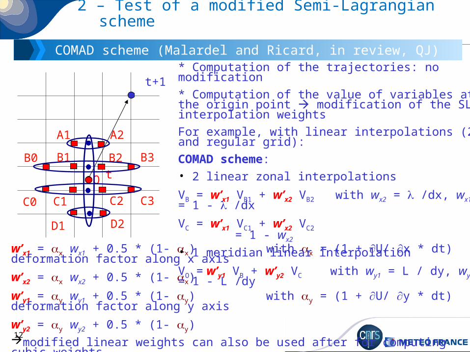
COMAD scheme (Malardel and Ricard, in review, QJ)
2 – Test of a modified Semi-Lagrangian scheme
t+1
t
B1 B2
C2C1
O
w’x1 = x wx1 + 0.5 * (1- x) with x = (1 + U/ x * dt) deformation factor along x axis
w’x2 = x wx2 + 0.5 * (1- x)
w’y1 = y wy1 + 0.5 * (1- y) with y = (1 + U/ y * dt) deformation factor along y axis
w’y2 = y wy2 + 0.5 * (1- y)modified linear weights can also be used after for computing cubic weights
AROME uses quasi-cubic interpolations (2 linear, 3 cubic ones)
B0 B3
C3C0
A1 A2
D1 D2
* Computation of the trajectories: no modification
* Computation of the value of variables at the origin point modification of the SL interpolation weights
For example, with linear interpolations (2D and regular grid):
COMAD scheme:
• 2 linear zonal interpolations
VB = w’x1 VB1 + w’x2 VB2 with wx2 = /dx, wx1 = 1 - /dx
VC = w’x1 VC1 + w’x2 VC2 = 1 - wx2
• 1 meridian linear interpolation
VO = w’y1 VB + w’y2 VC with wy1 = L / dy, wy2 = 1 - L /dy

13
2 – Test of a modified Semi-Lagrangian scheme
Example: 30 June 2012
24-h precipitation (mm) from 00 UTC - Wind vectors at 10 m (m/s), 00 UTC 1 July
Less precipitationLess intense wind ahead of precipitation area
COMADOPER SL
14
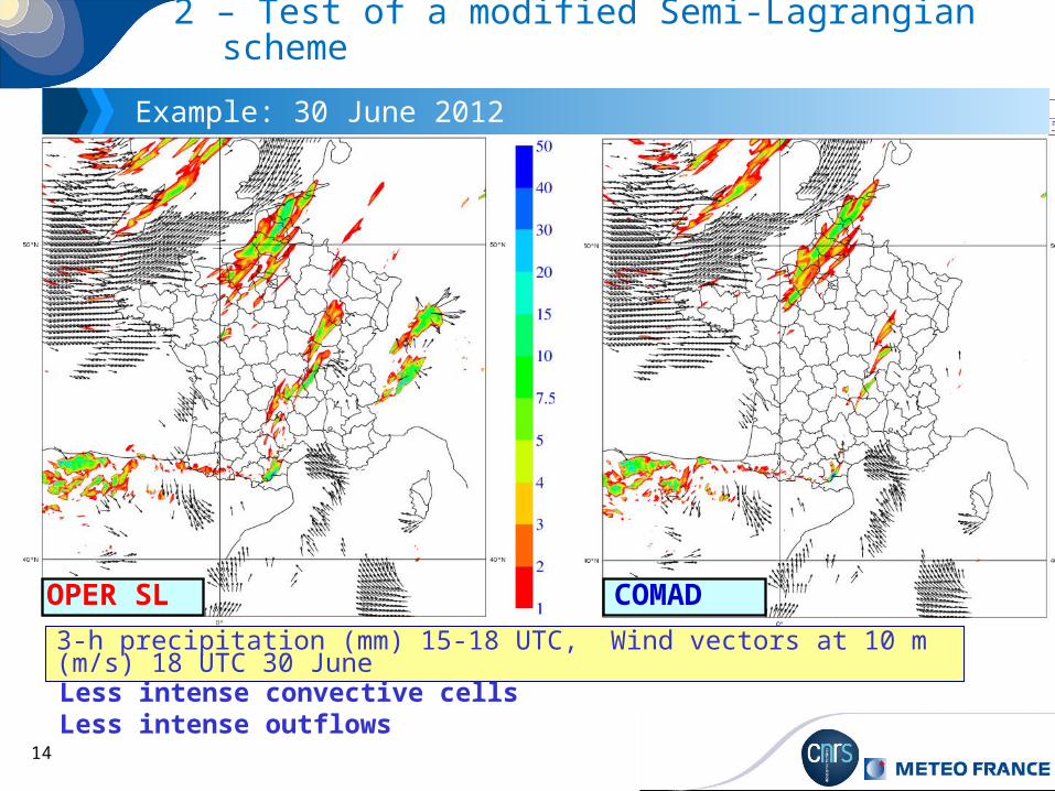
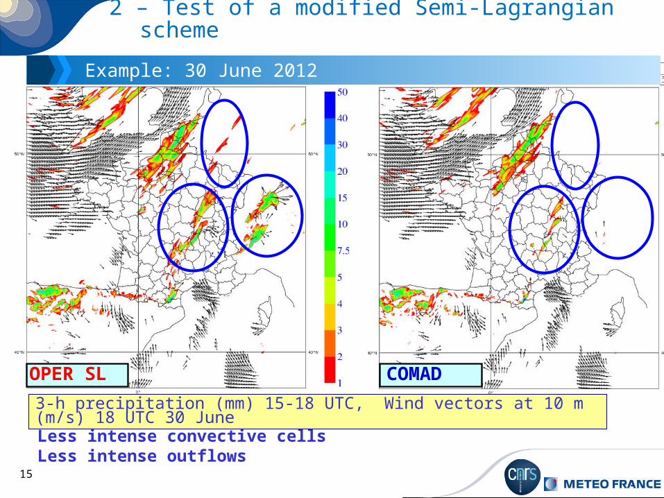
2 – Test of a modified Semi-Lagrangian scheme
Example: 30 June 2012
3-h precipitation (mm) 15-18 UTC, Wind vectors at 10 m (m/s) 18 UTC 30 June
Less intense convective cells Less intense outflows
COMADOPER SL
15
2 – Test of a modified Semi-Lagrangian scheme
Example: 30 June 2012
Less intense convective cells Less intense outflows
3-h precipitation (mm) 15-18 UTC, Wind vectors at 10 m (m/s) 18 UTC 30 June
COMADOPER SL
16
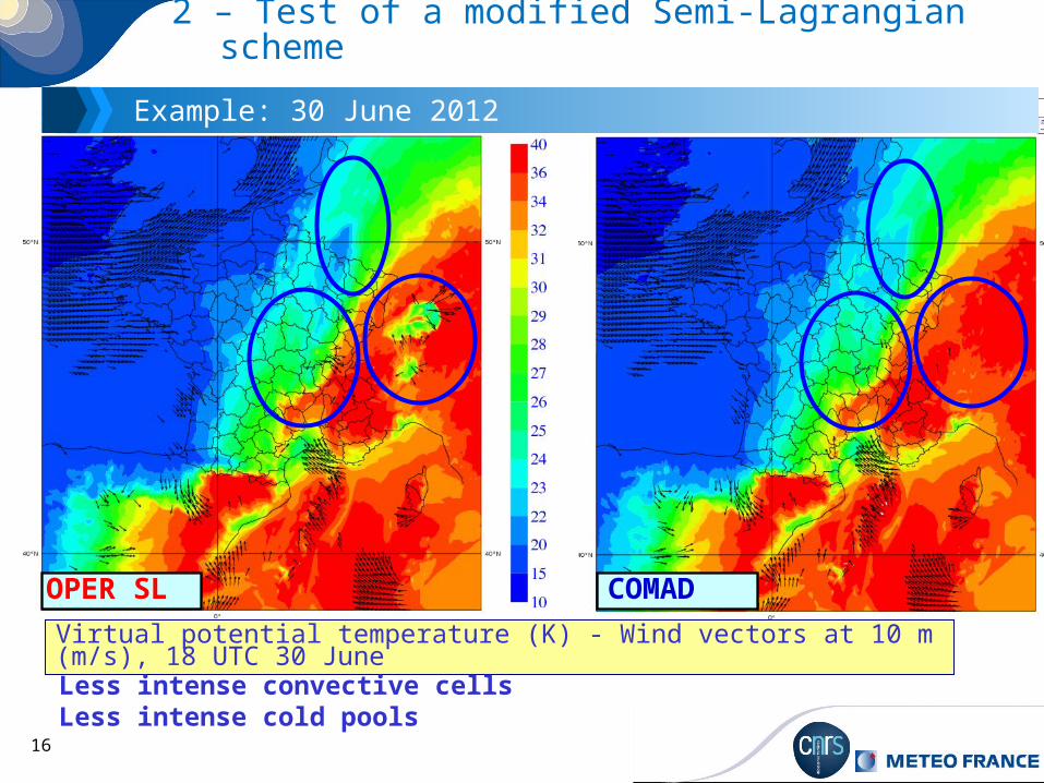
2 – Test of a modified Semi-Lagrangian scheme
Example: 30 June 2012
Virtual potential temperature (K) - Wind vectors at 10 m (m/s), 18 UTC 30 June
Less intense convective cells Less intense cold pools
COMADOPER SL
17
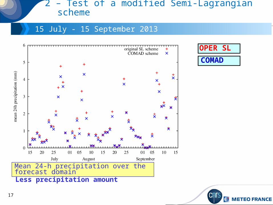
2 – Test of a modified Semi-Lagrangian scheme
15 July - 15 September 2013
Mean 24-h precipitation over the forecast domain
Less precipitation amount
COMAD
OPER SL

18
2 – Test of a modified Semi-Lagrangian scheme
15 July - 15 September 2013
Mean 24-h precipitation over the forecast domain
Less precipitation amountVariation between 1 and –26 %
19
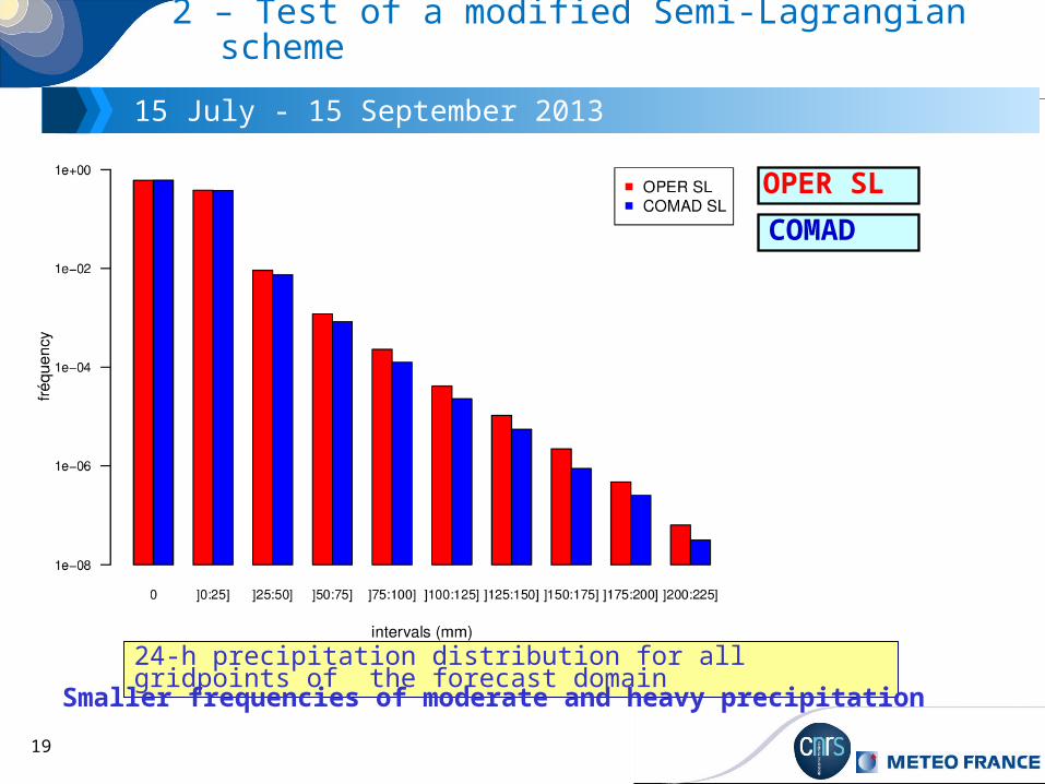
2 – Test of a modified Semi-Lagrangian scheme
15 July - 15 September 2013
24-h precipitation distribution for all gridpoints of the forecast domain
Smaller frequencies of moderate and heavy precipitation
COMAD
OPER SL
20
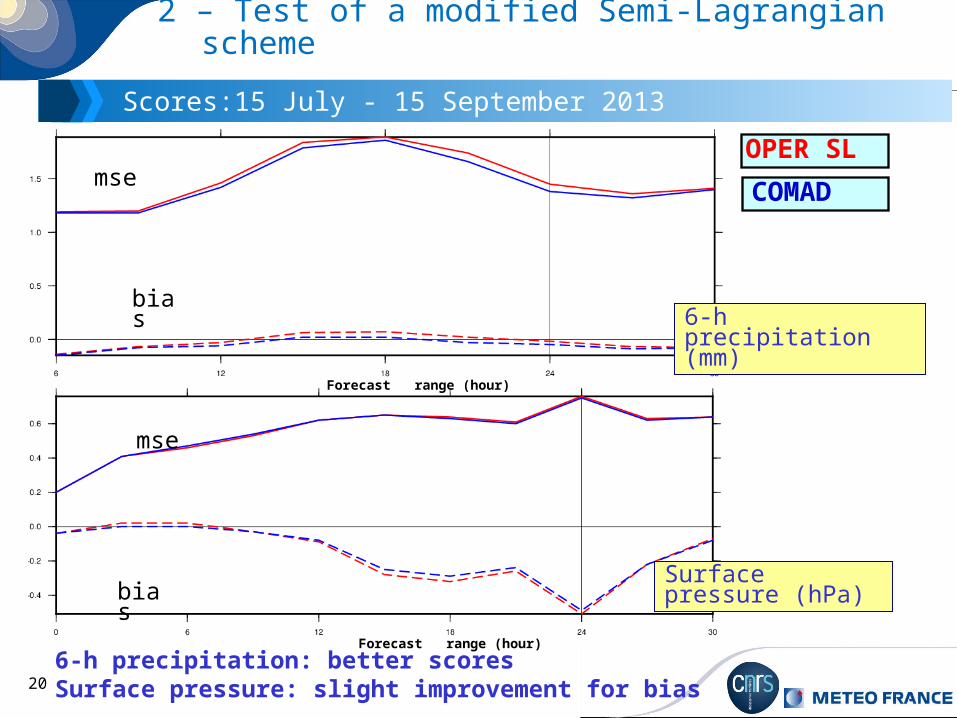
2 – Test of a modified Semi-Lagrangian scheme
Scores:15 July - 15 September 2013
6-h precipitation: better scoresSurface pressure: slight improvement for bias
6-h precipitation (mm)
Surface pressure (hPa)
Forecast range (hour)
Forecast range (hour)
bias
mse
bias
mse
COMAD
OPER SL
21
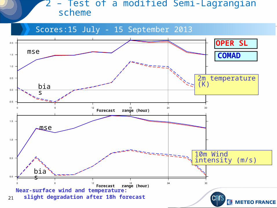
2 – Test of a modified Semi-Lagrangian scheme
Scores:15 July - 15 September 2013
Near-surface wind and temperature: slight degradation after 18h forecast
Forecast range (hour)
Forecast range (hour)
2m temperature (K)
10m Wind intensity (m/s)
bias
mse
bias
mse
COMAD
OPER SL
22
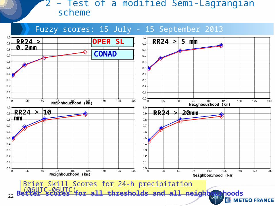
2 – Test of a modified Semi-Lagrangian scheme
Fuzzy scores: 15 July - 15 September 2013
Brier Skill Scores for 24-h precipitation (06UTC-06UTC) Better scores for all thresholds and all neighbourhoods
RR24 > 0.2mm RR24 > 5 mm
RR24 > 10 mm RR24 > 20mm
Neighbourhood (km) Neighbourhood (km)
Neighbourhood (km) Neighbourhood (km)
COMAD
OPER SL

23
2 – Test of a modified Semi-Lagrangian scheme
Fuzzy scores: 15 July - 15 September 2013
Brier Skill Scores for 6-h precipitation (12UTC-18UTC) Better scores for all thresholds and all neighbourhoods
RR6 > 0.5 mm RR6 > 2 mm
RR6 > 5 mm RR6 > 10mm
Neighbourhood (km) Neighbourhood (km)
Neighbourhood (km) Neighbourhood (km)
COMAD
OPER SL
24
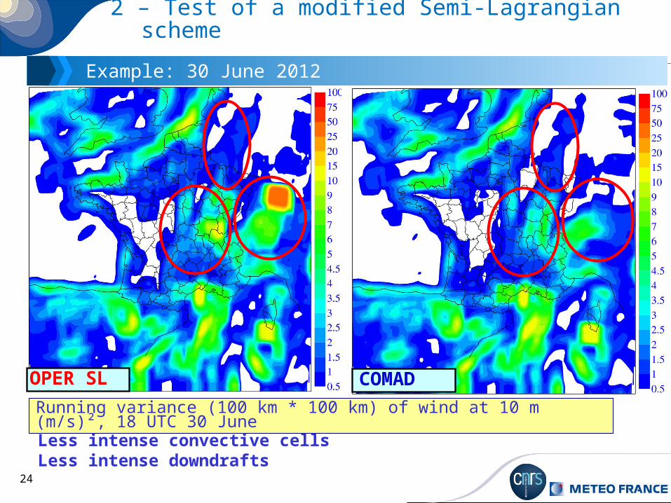
2 – Test of a modified Semi-Lagrangian scheme
Example: 30 June 2012
Running variance (100 km * 100 km) of wind at 10 m (m/s)², 18 UTC 30 June
Less intense convective cells Less intense downdrafts
COMADOPER SL

25
2 – Test of a modified Semi-Lagrangian scheme
15 July -15 September 2013
Running variance (100 km * 100 km)
(hourly averaged over the forecast domain and the period 15 July - 15 September 2013)
Less variance during the afternoon and eveningLess intense density currents under convective cells
10-m Wind (m²/s²)
10-m downdrafts (m²/s²)
925 hPa Virtual potential temperature (K²)
COMAD
OPER SL

26
2 – Test of a modified Semi-Lagrangian scheme
15 July -15 September 2013
Diurnal cycle of surface covered by convective cells (simulated reflectivities above 30 dBZ)
Less intense convective cells
COMAD
OPER SL

27
3 – Evaluation of AROME at kilometric resolution
Methodology
Smaller forecast domain
(720 points *720 points - 1.3km) (360 points *360 points - 2.5km)
Configuration:• for stability: ICI scheme (instead of 2TL SI scheme)• time step: 45s (instead of 60s)• initial conditions: dynamical adaptation from 2.5km 3DVAR Analysis• LBC: from operational AROME• better representation of the orography at 1.3km
Experiments Horizontal grid spacing Vertical levels
2.5km60 2.5 km 60 (21 levels < 2000m)
2.5km90 2.5 km 90 (33 levels < 2000m)1.3km90 1.3 km 90 (33 levels < 2000m)
1.3km90BC 1.3 km 90 (41 levels < 2000m)
Layer thickness (m)
L 60
L 90
L 90BC
28
3 – Evaluation of AROME at kilometric resolution
Methodology
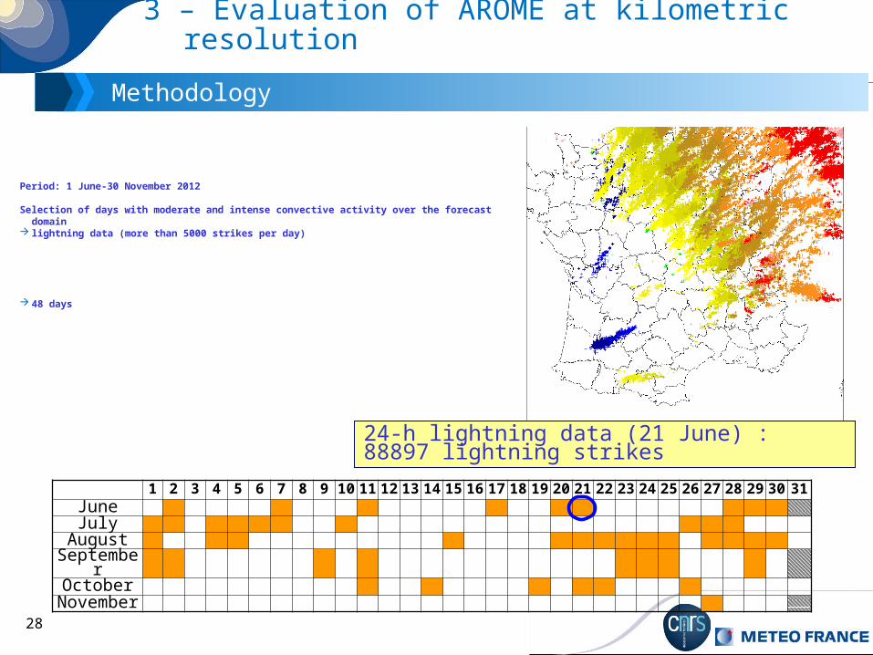
Period: 1 June-30 November 2012
Selection of days with moderate and intense convective activity over the forecast domain lightning data (more than 5000 strikes per day)
48 days
1 2 3 4 5 6 7 8 9 10 11 12 13 14 15 16 17 18 19 20 21 22 23 24 25 26 27 28 29 30 31
JuneJuly
AugustSeptember
OctoberNovember
24-h lightning data (21 June) : 88897 lightning strikes
29
3 – Evaluation of AROME at kilometric resolution
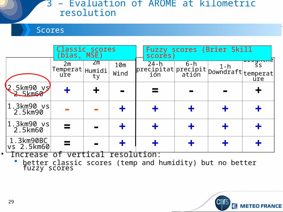
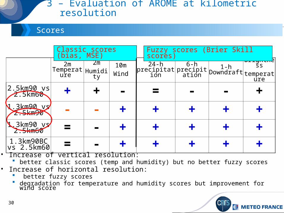
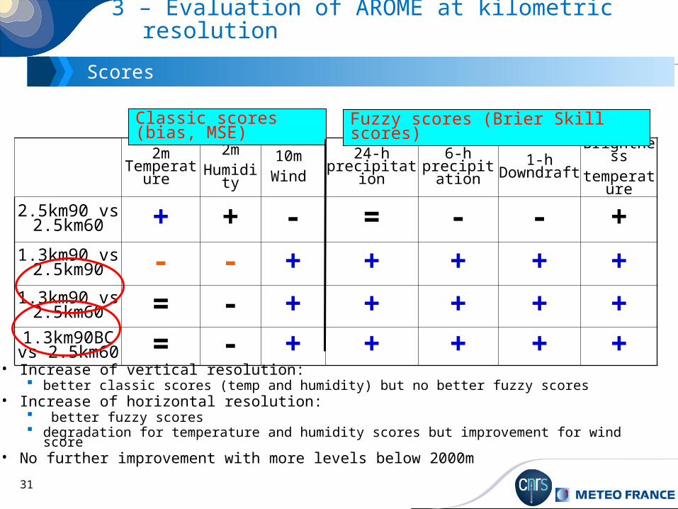
Scores
• Increase of vertical resolution: better classic scores (temp and humidity) but no better fuzzy scores
2m Temperature
2mHumidity
10m Wind
24-h precipitation
6-h precipitation
1-h Downdraft
Brightnesstemperature
2.5km90 vs 2.5km60 + + - = - - +
1.3km90 vs 2.5km90 - - + + + + +
1.3km90 vs 2.5km60 = - + + + + +
1.3km90BC vs 2.5km60 = - + + + + +
Classic scores (bias, MSE) Fuzzy scores (Brier Skill scores)
30
3 – Evaluation of AROME at kilometric resolution
Scores
• Increase of vertical resolution: better classic scores (temp and humidity) but no better fuzzy scores
• Increase of horizontal resolution: better fuzzy scores degradation for temperature and humidity scores but improvement for wind score
2m Temperature
2mHumidity
10m Wind
24-h precipitation
6-h precipitation
1-h Downdraft
Brightnesstemperature
2.5km90 vs 2.5km60 + + - = - - +
1.3km90 vs 2.5km90 - - + + + + +
1.3km90 vs 2.5km60 = - + + + + +
1.3km90BC vs 2.5km60 = - + + + + +
Classic scores (bias, MSE) Fuzzy scores (Brier Skill scores)
31
3 – Evaluation of AROME at kilometric resolution
Scores
• Increase of vertical resolution: better classic scores (temp and humidity) but no better fuzzy scores
• Increase of horizontal resolution: better fuzzy scores degradation for temperature and humidity scores but improvement for wind score
• No further improvement with more levels below 2000m
2m Temperature
2mHumidity
10m Wind
24-h precipitation
6-h precipitation
1-h Downdraft
Brightnesstemperature
2.5km90 vs 2.5km60 + + - = - - +
1.3km90 vs 2.5km90 - - + + + + +
1.3km90 vs 2.5km60 = - + + + + +
1.3km90BC vs 2.5km60 = - + + + + +
Classic scores (bias, MSE) Fuzzy scores (Brier Skill scores)

32
3 – Evaluation of AROME at kilometric resolution
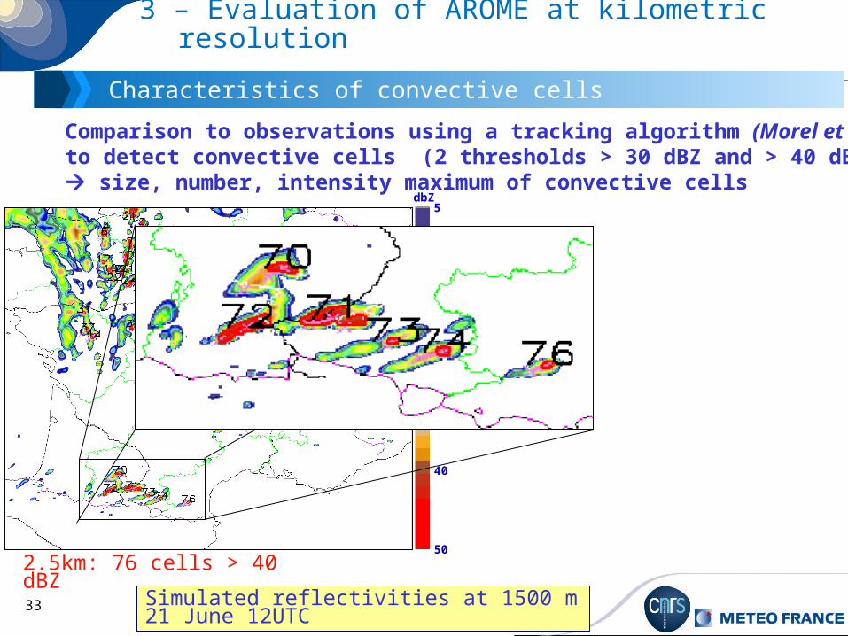
Characteristics of convective cells
Comparison to observations using a tracking algorithm (Morel et al., 2002) to detect convective cells (2 thresholds > 30 dBZ and > 40 dBZ) size, number, intensity maximum of convective cells
Simulated reflectivities at 1500 m 21 June 12UTC
2.5km: 76 cells > 40 dBZ
5dbZ
10
15
20
30
50
40
33
5dbZ
10
15
20
30
50
40
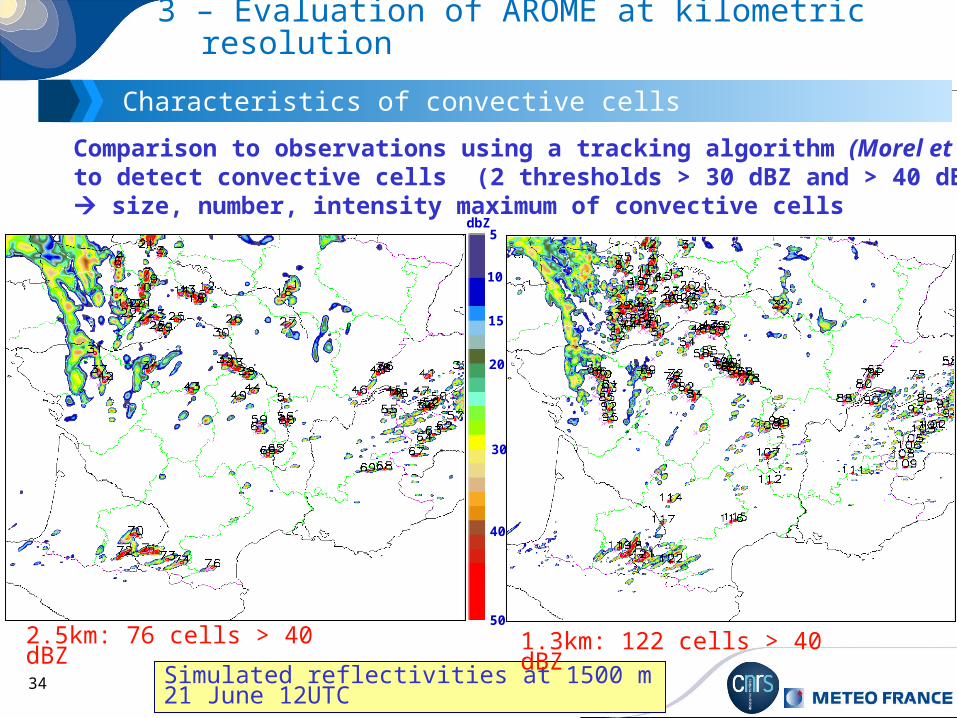
3 – Evaluation of AROME at kilometric resolution
Characteristics of convective cells
Simulated reflectivities at 1500 m 21 June 12UTC
2.5km: 76 cells > 40 dBZ
Comparison to observations using a tracking algorithm (Morel et al., 2002) to detect convective cells (2 thresholds > 30 dBZ and > 40 dBZ) size, number, intensity maximum of convective cells
34
3 – Evaluation of AROME at kilometric resolution
Characteristics of convective cells
Simulated reflectivities at 1500 m 21 June 12UTC
2.5km: 76 cells > 40 dBZ 1.3km: 122 cells > 40 dBZ
5dbZ
10
15
20
30
50
40
Comparison to observations using a tracking algorithm (Morel et al., 2002) to detect convective cells (2 thresholds > 30 dBZ and > 40 dBZ) size, number, intensity maximum of convective cells

35
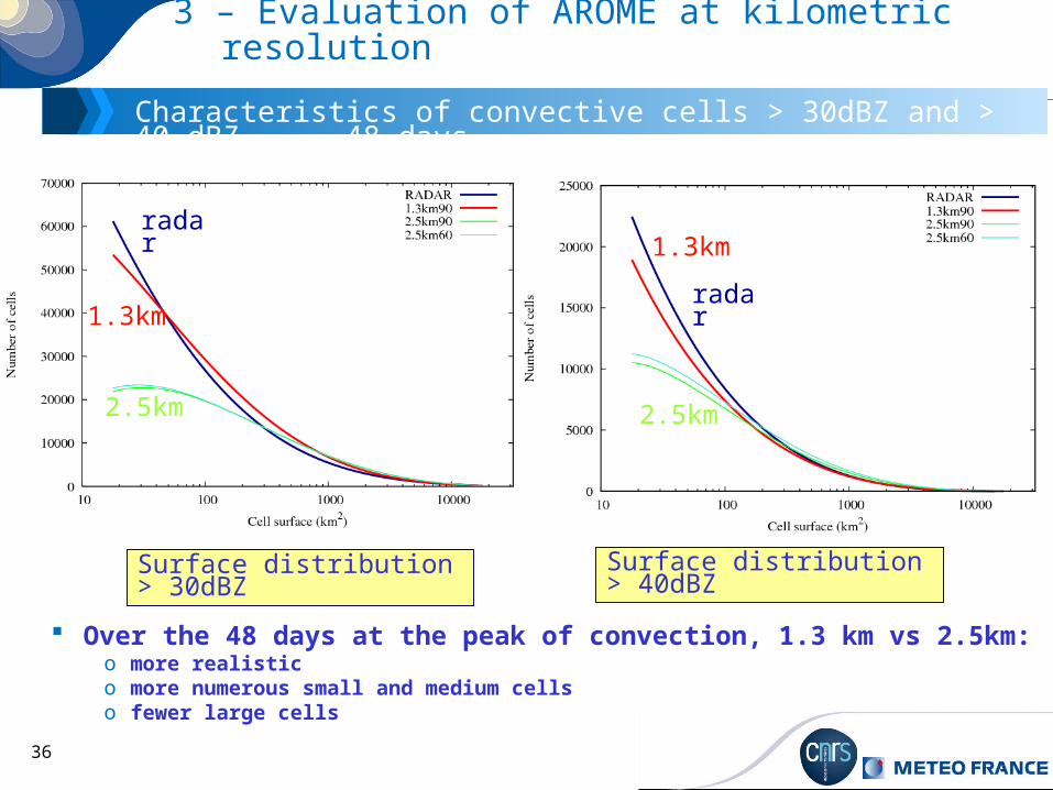
3 – Evaluation of AROME at kilometric resolution
Characteristics of convective cells > 40 dBZ - 21 June
1.3 km vs 2.5km:o more cellso more numerous small cellso fewer large cells o more realistic
Time evolution of cell number Surface distribution
radar
1.3kmradar
1.3km
2.5km2.5km
36
3 – Evaluation of AROME at kilometric resolution
Characteristics of convective cells > 30dBZ and > 40 dBZ - 48 days
Over the 48 days at the peak of convection, 1.3 km vs 2.5km:o more realistico more numerous small and medium cells o fewer large cells
Surface distribution > 30dBZ Surface distribution > 40dBZ
radar
1.3km
2.5km
radar
1.3km
2.5km
37
Conclusion
• Increase of horizontal grid spacing (1.3km versus 2.5km): more realistic number of cells more numerous small cells, fewer large cells reduction of precipitation amount better fuzzy scores (for precipitation, brightness temperature, downdrafts …)
• Use of the modified SL scheme (COMAD versus original SL scheme) less intense convective cells improvement of QPF, less amount better fuzzy scores for precipitation test on other periods: June 2012, January 2013 (frontal precipitation)
Test of the modified SL scheme at 1.3km
38

39
2 – Test of a modified Semi-Lagrangian scheme
Fuzzy scores: 15 July - 15 September 2013
Brier Skill Scores for brightness temperature 10.8 m (forecast range 18 UTC)
For peak of convection: better scores in particular for lower temperature thresholds better representation of the high clouds
Neighbourhood 20 km
Temperature thresholds (K)
Neighbourhood 52 km
Temperature thresholds (K)
COMAD
OPER SL

40
2 – Test of a modified Semi-Lagrangian scheme
1-31 January 2013
Mean 24-h precipitation over the forecast domain
Less impact on frontal precipitation
COMAD
OPER SL

41
2 – Test of a modified Semi-Lagrangian scheme
1-31 January 2013
Mean 24-h precipitation over the forecast domain
Less impact on frontal precipitationVariation between 1 and –5 %
42
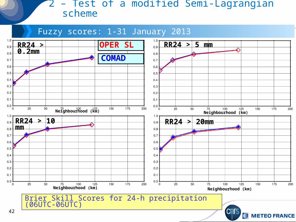
2 – Test of a modified Semi-Lagrangian scheme
Fuzzy scores: 1-31 January 2013
Brier Skill Scores for 24-h precipitation (06UTC-06UTC)
RR24 > 0.2mm RR24 > 5 mm
RR24 > 10 mm RR24 > 20mm
Neighbourhood (km) Neighbourhood (km)
Neighbourhood (km) Neighbourhood (km)
COMAD
OPER SL

43
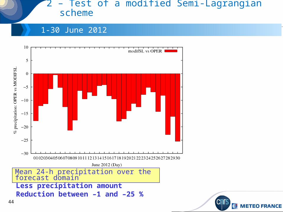
2 – Test of a modified Semi-Lagrangian scheme
1-30 June 2012
Mean 24-h precipitation over the forecast domain
Less precipitation amount
OPER
MODIFSL
44
2 – Test of a modified Semi-Lagrangian scheme
1-30 June 2012
Mean 24-h precipitation over the forecast domain
Less precipitation amountReduction between –1 and –25 %
45
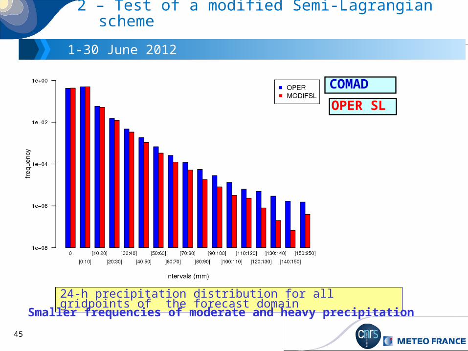
2 – Test of a modified Semi-Lagrangian scheme
1-30 June 2012
24-h precipitation distribution for all gridpoints of the forecast domain
Smaller frequencies of moderate and heavy precipitation
COMAD
OPER SL
46
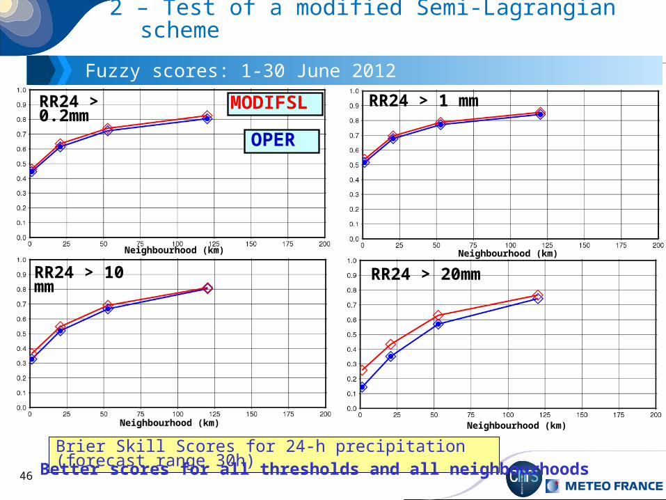
2 – Test of a modified Semi-Lagrangian scheme
Fuzzy scores: 1-30 June 2012
Brier Skill Scores for 24-h precipitation (forecast range 30h) Better scores for all thresholds and all neighbourhoods
OPER
MODIFSLRR24 > 0.2mm RR24 > 1 mm
RR24 > 10 mm RR24 > 20mm
Neighbourhood (km) Neighbourhood (km)
Neighbourhood (km) Neighbourhood (km)
47
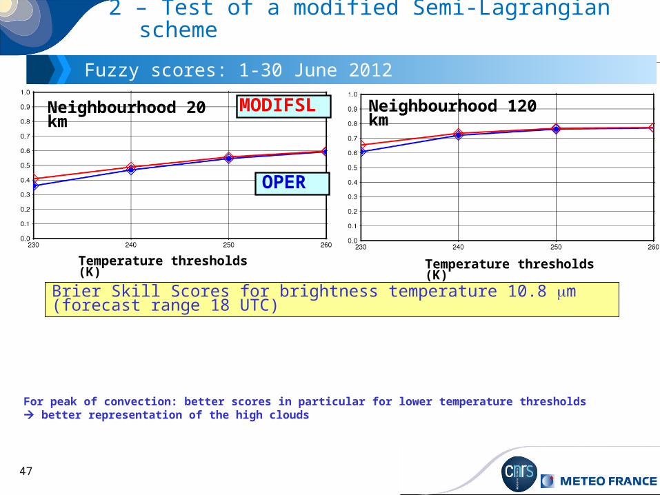
2 – Test of a modified Semi-Lagrangian scheme
Fuzzy scores: 1-30 June 2012
Brier Skill Scores for brightness temperature 10.8 m (forecast range 18 UTC)
For peak of convection: better scores in particular for lower temperature thresholds better representation of the high clouds
OPER
MODIFSLNeighbourhood 20 km
Temperature thresholds (K)
Neighbourhood 120 km
Temperature thresholds (K)
48
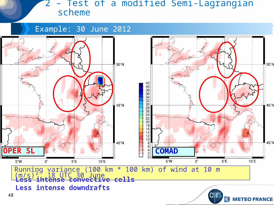
2 – Test of a modified Semi-Lagrangian scheme
Example: 30 June 2012
Running variance (100 km * 100 km) of wind at 10 m (m/s)², 18 UTC 30 June
Less intense convective cells Less intense downdrafts
COMADOPER SL

49
2 – Test of a modified Semi-Lagrangian scheme
Example: 30 June 2012
Running variance (100 km * 100 km) of downdrafts at 10 m (m/s)², 18 UTC 30 June
Less intense convective cells Less intense downdrafts
COMADOPER SL

50
2 – Test of a modified Semi-Lagrangian scheme
Example: 30 June 2012
Running variance (100 km * 100 km) of 925 hPa ϴv at 10 m (K)², 18 UTC 30 June
Less intense convective cells Less intense downdrafts
COMADOPER SL

51
3 – Evaluation of AROME at kilometric resolution
Characteristics of convective cells > 40 dbZ - 21 June
Time step impact:o 30s: slightly more cells, in particular small cellso 60s: slightly less cells in particular small cells
Time evolution of cell number Surface distribution

52
3 – Evaluation of AROME at kilometric resolution
Characteristics of convective cells > 40 dbZ - 21 June
Diffusion impact:o Without spectral diffusion: sightly more cellso Spectral diffusion constant on vertical: weak impact o Without SLHD: more cells
Time evolution of cell number Surface distribution
Related Documents