1 Lecture 3 Uninformed Search. 2 Complexity Recap (app.A) We often want to characterize algorithms independent of their implementation. “This algorithm.

1

Lecture 3

Uninformed Search

2

Complexity Recap (app.A)• We often want to characterize algorithms independent of their implementation.

• “This algorithm took 1 hour and 43 seconds on my laptop”.Is not very useful, because tomorrow computers are faster.

• Better is: “This algorithm takes O(nlog(n)) time to run and O(n) to store”. because this statement is abstracts away from irrelevant details.

Time(n) = O(f(n)) means: Time(n) < constant x f(n) for n>n0 for some n0Space(n) idem.

n is some variable which characterizes the size of the problem,e.g. number of data-points, number of dimensions, branching-factorof search tree, etc.

• Worst case analysis versus average case analyis

3

Uninformed search strategies

Uninformed: While searching you have no clue whether one non-goal state is better than any other. Your search is blind. You don’t know if your current exploration is likely to be fruitful.

Various blind strategies: Breadth-first search Uniform-cost search Depth-first search Iterative deepening search

4

Breadth-first search

Expand shallowest unexpanded node Fringe: nodes waiting in a queue to be

explored Implementation:

fringe is a first-in-first-out (FIFO) queue, i.e., new successors go at end of the queue.

Is A a goal state?

5

Breadth-first search

Expand shallowest unexpanded node Implementation:

fringe is a FIFO queue, i.e., new successors go at end

Expand:fringe = [B,C]

Is B a goal state?

6

Breadth-first search

Expand shallowest unexpanded node Implementation:

fringe is a FIFO queue, i.e., new successors go at end

Expand:fringe=[C,D,E]

Is C a goal state?

7

Breadth-first search

Expand shallowest unexpanded node Implementation:

fringe is a FIFO queue, i.e., new successors go at end

Expand:fringe=[D,E,F,G]

Is D a goal state?

8

ExampleBFS

9

Properties of breadth-first search

Complete? Yes it always reaches goal (if b is finite)

Time? 1+b+b2+b3+… +bd + (bd+1-b)) = O(bd+1) (this is the number of nodes we

generate) Space? O(bd+1) (keeps every node in memory, either in fringe or on a path to fringe). Optimal? Yes (if we guarantee that deeper

solutions are less optimal, e.g. step-cost=1).

Space is the bigger problem (more than time)

10

Uniform-cost search

Breadth-first is only optimal if step costs is increasing with depth (e.g. constant). Can we guarantee optimality for any step cost?

Uniform-cost Search: Expand node with smallest path cost

g(n).

11

Uniform-cost search

Implementation: fringe = queue ordered by path costEquivalent to breadth-first if all step costs all equal.

Complete? Yes, if step cost ≥ ε (otherwise it can get stuck in infinite loops)

Time? # of nodes with path cost ≤ cost of optimal solution.

Space? # of nodes on paths with path cost ≤ cost of optimal solution.

Optimal? Yes, for any step cost.

12

S B

A D

E

C

F

G

1 20

2

3

4 8

6 11

straight-line distances

h(S-G)=10h(A-G)=7h(D-G)=1h(F-G)=1h(B-G)=10h(E-G)=8h(C-G)=20

The graph above shows the step-costs for different paths going from the start (S) to the goal (G). On the right you find the straight-line distances.

Use uniform cost search to find the optimal path to the goal.

Exercise for at home

13

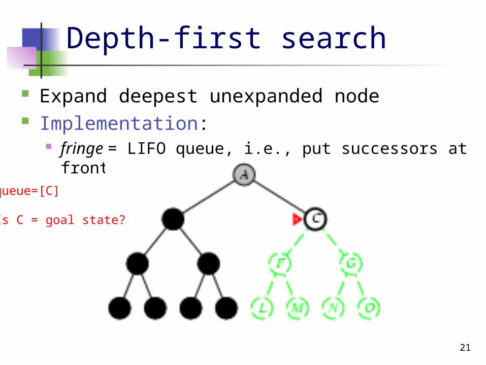
Depth-first search

Expand deepest unexpanded node Implementation:

fringe = Last In First Out (LIPO) queue, i.e., put successors at front

Is A a goal state?

14

Depth-first search

Expand deepest unexpanded node Implementation:

fringe = LIFO queue, i.e., put successors at front

queue=[B,C]

Is B a goal state?

15

Depth-first search

Expand deepest unexpanded node Implementation:

fringe = LIFO queue, i.e., put successors at front

queue=[D,E,C]

Is D = goal state?

16

Depth-first search

Expand deepest unexpanded node Implementation:

fringe = LIFO queue, i.e., put successors at front

queue=[H,I,E,C]

Is H = goal state?

17

Depth-first search

Expand deepest unexpanded node Implementation:

fringe = LIFO queue, i.e., put successors at front

queue=[I,E,C]

Is I = goal state?

18

Depth-first search

Expand deepest unexpanded node Implementation:

fringe = LIFO queue, i.e., put successors at front

queue=[E,C]

Is E = goal state?

19

Depth-first search

Expand deepest unexpanded node Implementation:

fringe = LIFO queue, i.e., put successors at front

queue=[J,K,C]

Is J = goal state?

20

Depth-first search

Expand deepest unexpanded node Implementation:

fringe = LIFO queue, i.e., put successors at front

queue=[K,C]

Is K = goal state?

21

Depth-first search

Expand deepest unexpanded node Implementation:

fringe = LIFO queue, i.e., put successors at front

queue=[C]

Is C = goal state?

22

Depth-first search

Expand deepest unexpanded node Implementation:

fringe = LIFO queue, i.e., put successors at front

queue=[F,G]

Is F = goal state?

23

Depth-first search

Expand deepest unexpanded node Implementation:

fringe = LIFO queue, i.e., put successors at front

queue=[L,M,G]

Is L = goal state?

24

Depth-first search

Expand deepest unexpanded node Implementation:

fringe = LIFO queue, i.e., put successors at front

queue=[M,G]

Is M = goal state?

26

Properties of depth-first search

Complete? No: fails in infinite-depth spaces Can modify to avoid repeated states along path Time? O(bm) with m=maximum depth terrible if m is much larger than d

but if solutions are dense, may be much faster than breadth-first

Space? O(bm), i.e., linear space! (we only need to

remember a single path + expanded unexplored nodes) Optimal? No (It may find a non-optimal goal first)

A

B C

27

Iterative deepening search

• To avoid the infinite depth problem of DFS, we can decide to only search until depth L, i.e. we don’t expand beyond depth L. Depth-Limited Search

• What of solution is deeper than L? Increase L iteratively. Iterative Deepening Search

• As we shall see: this inherits the memory advantage of Depth-First search, and is better in terms of time complexity than Breadth first search.

28

Iterative deepening search L=0

29

Iterative deepening search L=1

30

Iterative deepening search L=2

31

Iterative Deepening Search L=3

32

Iterative deepening search Number of nodes generated in a depth-limited search

to depth d with branching factor b: NDLS = b0 + b1 + b2 + … + bd-2 + bd-1 + bd

Number of nodes generated in an iterative deepening search to depth d with branching factor b:

NIDS = (d+1)b0 + d b1 + (d-1)b2 + … + 3bd-2 +2bd-1 + 1bd =

For b = 10, d = 5, NDLS = 1 + 10 + 100 + 1,000 + 10,000 + 100,000 = 111,111 NIDS = 6 + 50 + 400 + 3,000 + 20,000 + 100,000 = 123,450 NBFS = ............................................................................................ = 1,111,100

1( ) ( )d dO b O b

BFS

33

Properties of iterative deepening search

Complete? Yes Time? O(bd) Space? O(bd) Optimal? Yes, if step cost = 1 or

increasing function of depth.

34

Example IDS

35

Bidirectional Search

Idea simultaneously search forward from S and backwards

from G stop when both “meet in the middle” need to keep track of the intersection of 2 open sets of

nodes What does searching backwards from G mean

need a way to specify the predecessors of G this can be difficult, e.g., predecessors of checkmate in chess?

which to take if there are multiple goal states? where to start if there is only a goal test, no explicit list?

36

Bi-Directional Search

Complexity: time and space complexity are: / 2( )dO b

37

Summary of algorithms

even completeif step cost is notincreasing with depth.

preferred uninformedsearch strategy

38

Repeated states

Failure to detect repeated states can turn a linear problem into an exponential one!

39

Solutions to Repeated States

Graph search never generate a state generated before

must keep track of all possible states (uses a lot of memory)

e.g., 8-puzzle problem, we have 9! = 362,880 states approximation for DFS/DLS: only avoid states in

(limited memory).

S

B

C

S

B C

SC B S

State SpaceExample of a Search Tree

optimal but memory inefficient

40

Summary

Problem formulation usually requires abstracting away real-world details to define a state space that can feasibly be explored

Variety of uninformed search strategies

Iterative deepening search uses only linear space and not much more time than other uninformed algorithms

http://www.cs.rmit.edu.au/AI-Search/Product/http://aima.cs.berkeley.edu/demos.html (for more demos)