1 Laplace transformation. 2 The Laplace transform is a mathematical technique used for solving linear differential equations (apparent zero order and.

1

Laplace transformation

2

Laplace transformation

• The Laplace transform is a mathematical technique used for solving linear differential equations (apparent zero order and first order) and hence is applicable to the solution of many equations used for pharmacokinetic analysis.

3

Laplace transformation procedure

1. Write the differential equation

2. Take the Laplace transform of each differential equation using a few transforms (using table in the next slide)

3. Use some algebra to solve for the Laplace of the system component of interest

4. Finally the 'anti'-Laplace for the component is determined from tables

4

Important Laplace transformation (used in step 2)

Expression Transform

dX/dt

K (constant)

X (variable)

K∙X (K is constant)

0XXs

s

K

X

XK

where s is the laplace operator, is the laplace integral

, and X0 is the amount at time zero

X

5

Anti-laplce table (used in step 4)

6

Anti-laplce table continued (used in step 4)

7

Laplace transformation: example

• The differential equation that describes the change in blood concentration of drug X is:

Derive the equation that describe the amount of drug X??

kXdt

dX

8


1. Write the differential equation:

2. Take the Laplace transform of each differential equation:

kXdt

dX

XkXXs 0

9


3. Use some algebra to solve for the Laplace of the system component of interest

4. Finally the 'anti'-Laplace for the component is determined from tables

sk

XX

0

kteXtX 0)(

10


• The derived equation represent the equation for IV bolus one compartment

11

Continuous intravenous infusion(one-compartment model)

Dr Mohammad Issa

12

Theory of intravenous infusion• The drug is administered at a selected or

calculated constant rate (K0) (i.e. dX/dt), the units of this input rate will be those of mass per unit time (e.g.mg/hr).

• The constant rate can be calculated from the concentration of drug solution and the flow rate of this solution, For example, the concentration of drug solution is 1% (w/v) and this solution is being infused at the constant rate of 10mL/hr (solution flow rate). So 10mL of solution will contain 0.1 g (100 mg) drug.

• The infusion rate (K0) equals to the solution flow rate multiplied by the concentration

• In this example, the infusion rate will be 10mL/hr multiplied by 100 mg/10 mL, or 100mg/hr. The elimination of drug from the body follows a first

13

IV infusion

0

5

10

15

20

25

30

35

0 5 10 15 20 25 30 35 40

Time

Co

nce

ntr

atio

n

During infusion Post infusion

14

IV infusion: during infusion

0

5

10

15

20

25

30

35

0 5 10 15 20 25 30 35 40

Time

Co

nce

ntr

atio

n

where K0 is the infusion rate, K is the elimination rate constant, and Vd is the volume of distribution

)1( eKto

K

KX

)1( eKto

pKVd

KC

15

Steady state

0

5

10

15

20

25

30

35

0 5 10 15 20 25 30 35 40

Time

Co

nce

ntr

atio

n

≈ steady state concentration (Css)

KVd

KC

oss

16

Steady state

• At steady state the input rate (infusion rate) is equal to the elimination rate.

• This characteristic of steady state is valid for all drugs regardless to the pharmacokinetic behavior or the route of administration.

17

Fraction achieved of steady state concentration (Fss)

)1( eKto

pKVd

KC

since , previous equation can

be represented as:

KVdKC oss

)1( eKt

ssp CC

eKt

ss

p

ss C

CF

1

5.0

2/1

2

111

)2ln( t

t

tt

ss eF

18

Fraction achieved of steady state concentration (Fss)

5.0

2

11

t

t

ssF

or e

Kt

ssF1

19

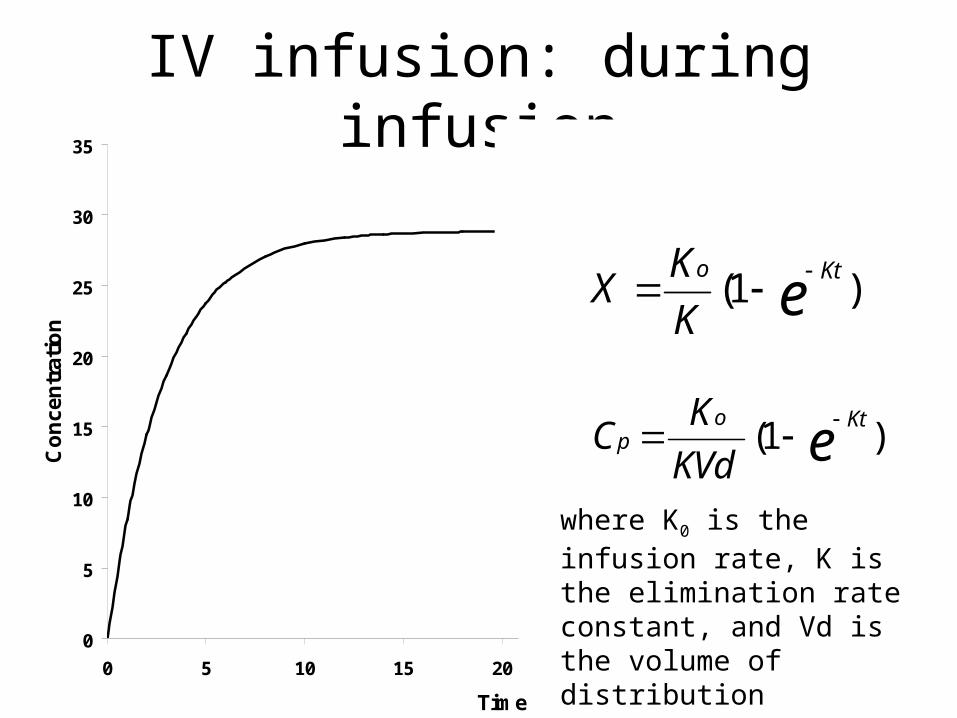
Time needed to achieve steady state

time needed to get to a certain fraction of steady state depends on the half life of the drug (not the infusion rate)

)1ln(44.1 5.0 SSFtt

20

Example

• What is the minimum number of half lives needed to achieve at least 95% of steady state?

• At least 5 half lives (not 4) are needed to get to 95% of steady state

0.55.05.0

5.0

t53.4)95.01ln(44.1

)1ln(44.1

tt

Ftt SS

21

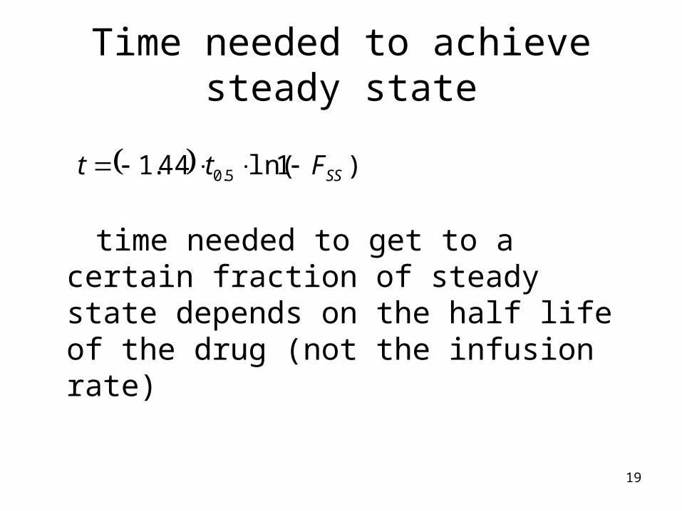
Example

• A drug with an elimination half life of 10 hrs. Assuming that it follows a one compartment pharmacokinetics, fill the following table:

22

Example

Time Fss

10

30

50

70

90

23

Example

TimeNumber of elapsed

half-livesFss

10 1 0.5

30 3 0.875

50 5 0.969

70 7 0.992

90 9 0.998

24

IV infusion + Loading IV bolus• During constant rate IV administration, the drug accumulates

until steady state is achieved after five to seven half-lives

• This can constitute a problem when immediate drug effect is required and immediate achievement of therapeutic drug concentrations is necessary such as in emergency situations

• In this ease, administration of a loading dose will be necessary. The loading dose is an IV holus dose administered at the time of starting the IV infusion to achieve faster approach to steady state. So administration of an IV loading dose and starting the constant rate IV infusion simultaneously can rapidly produce therapeutic drug concentration. The loading dose is chosen to produce Plasma concentration similar or close to the desired plasma concentration that will be achieved by the IV infusion at steady state

25

IV infusion + Loading IV bolus

26


• To achieve a target steady state conc (Css) the following equations can be used:– For the infusion rate:

– For the loading dose:ssCClK 0

ssCVdLD

27


• The conc. resulting from both the bolus and the infusion can be described as:

Ctotal =Cinfusion + Cbolus

28

IV infusion + Loading IV bolus: Example

• Derive the equation that describe plasma concentration of a drug with one compartment PK resulting from the administration of an IV infusion (K0= Css∙Cl ) and a loading bolus (LD= Css∙Vd) that was given at the start of the infusion

29



• Cinfusion:

• Cbolus:

)e(1CC tKssinfusion

tKtKsstK0bolus ee

Ce

XC

ssCVd

Vd

Vd

30



sstotal

tKss

tKsssstotal

tKss

tKsstotal

CC

eCeCCC

eC)e(1CC

31

Co

nce

ntr

atio

nC

on

cen

trat

ion

Co

nce

ntr

atio

nC

on

cen

trat

ion

Half-lives

Half-lives

Half-lives

Half-lives

Case A

Infusion alone

(K0= Css∙Cl)

Case BInfusion (K0= Css∙Cl)

loading bolus (LD= Css∙Vd)

Case DInfusion (K0= Css∙Cl)

loading bolus (LD< Css∙Vd)

Case CInfusion (K0= Css∙Cl)

loading bolus (LD > Css∙Vd)

Scenarios with different LD

32

Changing Infusion RatesC

on

cen

trat

ion

Half-lives5-7 half-lives are needed to get to

steady state

Increasing the infusion rate results in a new steady state

conc. 5-7 half-lives are needed to get to the new

steady state conc

Decreasing the infusion rate results in a new steady state conc. 5-7 half-lives are needed to get to

the new steady state conc

33

Changing Infusion Rates

• The rate of infusion of a drug is sometimes changed during therapy because of excessive toxicity or an inadequate therapeutic response. If the object of the change is to produce a new plateau, then the time to go from one plateau to another—whether higher or lower—depends solely on the half-life of the drug.

34

Post infusion phase

0

5

10

15

20

25

30

35

0 5 10 15 20 25 30 35 40

Time

Co

nce

ntr

atio

n

During infusion Post infusion

C* (Concentration at the end of the infusion)

eKt

p CC *

35

Post infusion phase data

• Half-life and elimination rate constant calculation

• Volume of distribution estimation

36

Elimination rate constant calculation using post infusion data• K can be estimated using post infusion

data by:– Plotting log(Conc) vs. time– From the slope estimate K:

303.2

kSlope

37

Volume of distribution calculation using post infusion data

• If you reached steady state conc (C* = CSS):

• where k is estimated as described in the previous slide

ssss CK

KVd

VdK

KC

00

38

Volume of distribution calculation using post infusion data

• If you did not reached steady state (C* = CSS(1-e-kT)):

)1(*

)1(* 00 kTkT eCk

kVde

Vdk

kC

39

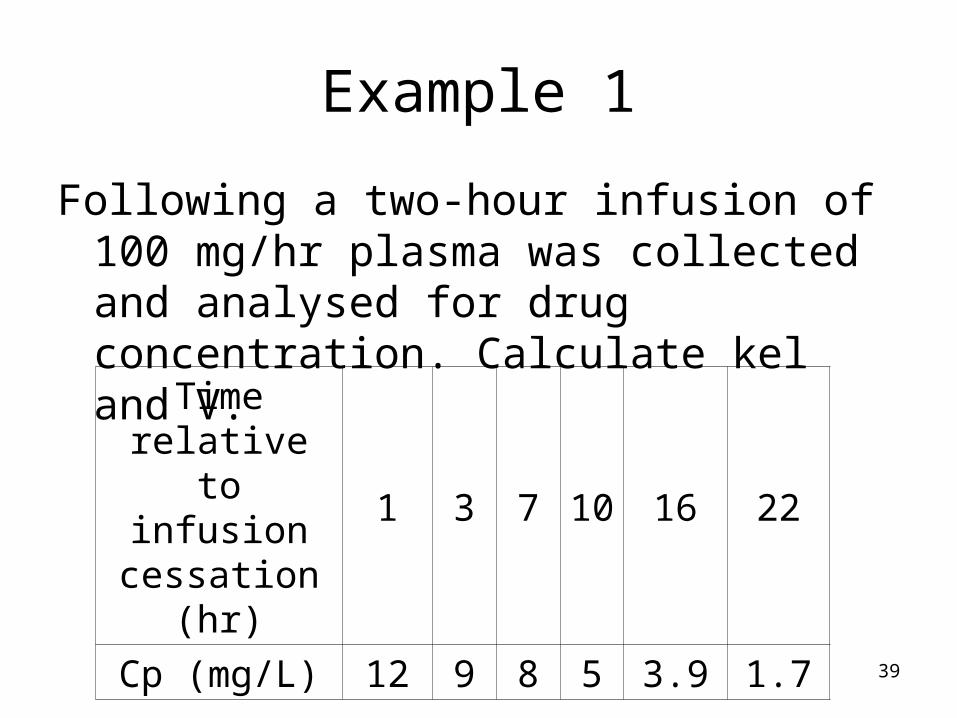
Example 1

Following a two-hour infusion of 100 mg/hr plasma was collected and analysed for drug concentration. Calculate kel and V.

Time relative to infusion

cessation (hr)1 3 7 10 16 22

Cp (mg/L) 12 9 8 5 3.9 1.7

40

Post infusion data

y = -0.0378x + 1.1144

R2 = 0.9664

0

0.2

0.4

0.6

0.8

1

1.2

0 5 10 15 20 25

Time (hr)

Lo

g(C

on

c) m

g/L

Time is the time after stopping the infusion

41

Example 1

• From the slope, K is estimated to be:

• From the intercept, C* is estimated to be:

1/hr 0.0870.03782.303Slope2.303k

mg/L 1310C*

1.1144interceptlog(C*)1.1144

42

Example 1

• Since we did not get to steady state:

L 14.1)e(1(13)(0.087)

100Vd

)e(1*Ck

kVd

20.087*

kT0

43

Example 2

• Estimate the volume of distribution (22 L), elimination rate constant (0.28 hr-1), half-life (2.5 hr), and clearance (6.2 L/hr) from the data in the following table obtained on infusing a drug at the rate of 50 mg/hr for 16 hours.

Time(hr)

0 2 4 6 10 12 15 16 18 20 24

Conc(mg/L)

0 3.48 5.47 6.6 7.6 7.8 8 8 4.6 2.62 0.85

44

Example 2

45

Example 2

1. Calculating clearance:

It appears from the data that the infusion has reached steady state:

(CP(t=15) = CP(t=16) = CSS)

L/hr 25.6mg/L 8

mg/hr 5000 SS

SS C

KCl

Cl

KC

46

Example 2

2. Calculating elimination rate constant and half life:

From the post infusion data, K and t1/2 can be estimated. The concentration in the post infusion phase is described according to:

where t1 is the time after stopping the infusion. Plotting log(Cp) vs. t1 results in the following:

1303.2)log()log(1 t

KCCeCC SSP

tKSSP

47

Example 2

y = -0.1218x + 0.9047

R2 = 1

-0.2

0

0.2

0.4

0.6

0.8

1

0 1 2 3 4 5 6 7 8 9

Post infusion time (hr)

log

(Co

nc

) (m

g/L

)

48

Example 2

K=-slope*2.303=0.28 hr-1

Half life = 0.693/K=0.693/0.28= 2.475 hr

3. Calculating volume of distribution:

L 3.22hr 28.0

L/hr 25.61-

K

ClVD

49

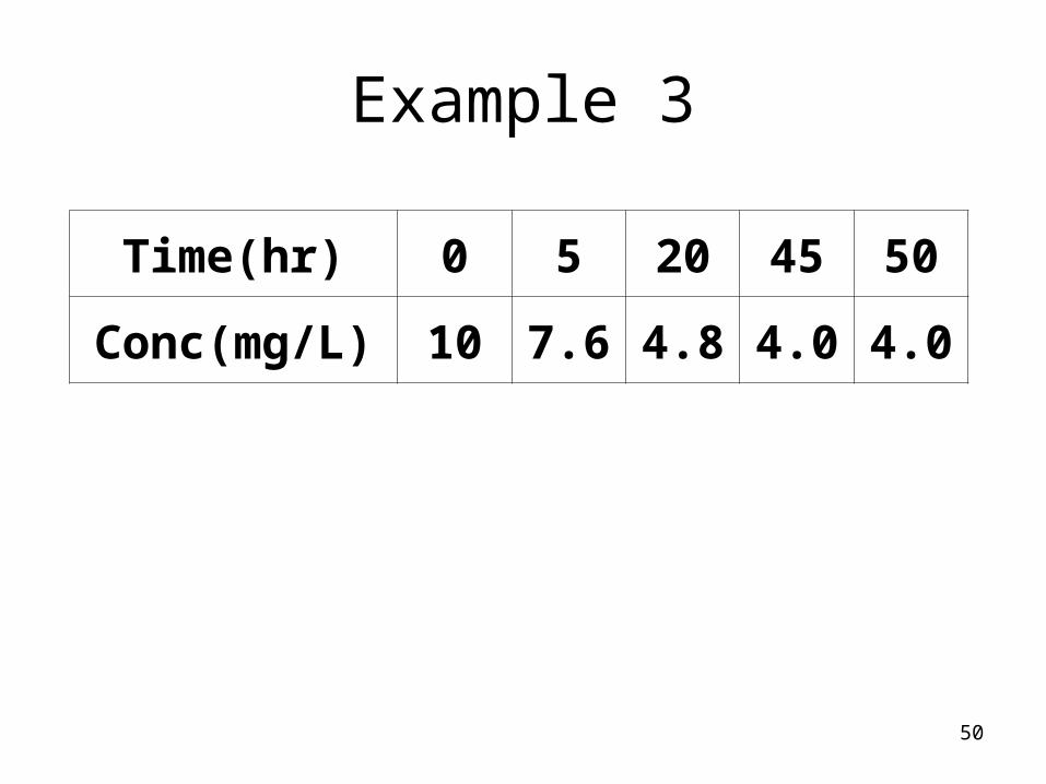
Example 3

• A drug that displays one compartment characteristics was administered as an IV bolus of 250 mg followed immediately by a constant infusion of 10 mg/hr for the duration of a study. Estimate the values of the volume of distribution (25 L), elimination rate constant (0.1hr-1), half-life (7), and clearance (2.5 L/hr) from the data in the following table

50

Example 3

Time(hr) 0 5 20 45 50

Conc(mg/L) 10 7.6 4.8 4.0 4.0

51

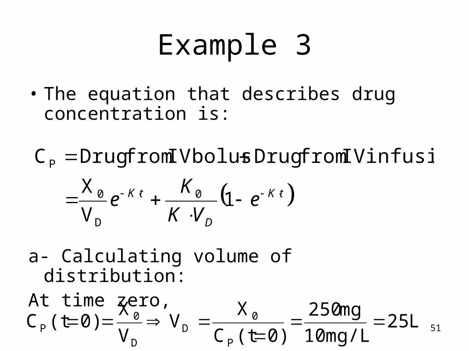
Example 3

• The equation that describes drug concentration is:

a- Calculating volume of distribution:At time zero,

tKD

tK eVK

Ke

1V

X

infusion IV from Drug bolus IV from DrugC

0

D

0

P

L 25mg/L 10

mg 250

0)(tC

XV

V

X0)(tC

P

0D

D

0P

52

Example 3

b- Calculating elimination rate constant and half life:

Since the last two concentrations (at time 45 and 50 hrs) are equal, it is assumed that a steady state situation has been achieved.

Half life = 0.693/K=0.693/0.1= 6.93 hr

1-00 hr 1.0L 25mg/L 4

mg/hr 10

DSSDSS VC

KK

VK

KC

53

Example 3

c- Calculating clearance:

L/hr 5.2251.0 DVKCl

54

Example 4

• For prolonged surgical procedures, succinylcholine is given by IV infusion for sustained muscle relaxation. A typical initial dose is 20 mg followed by continuous infusion of 4 mg/min. the infusion must be individualized because of variation in the kinetics of metabolism of suucinylcholine. Estimate the elimination half-lives of succinylcholine in patients requiring 0.4 mg/min and 4 mg/min, respectively, to maintain 20 mg in the body. (35 and 3.5 min)

55

Example 4

For the patient requiring 0.4 mg/min:

For the patient requiring 4 mg/min:

02/1

2/10

693.0

693.0 K

At

tK

K

KA SSo

ss

min 65.344.0

)693.0)(20(693.0

02/1

K

At SS

min 465.34

)693.0)(20(693.0

02/1

K

At SS

56

Example 5

A drug is administered as a short term infusion. The average pharmacokinetic parameters for this

drug are:

K = 0.40 hr-1

Vd = 28 L

This drug follows a one-compartment body model.

57

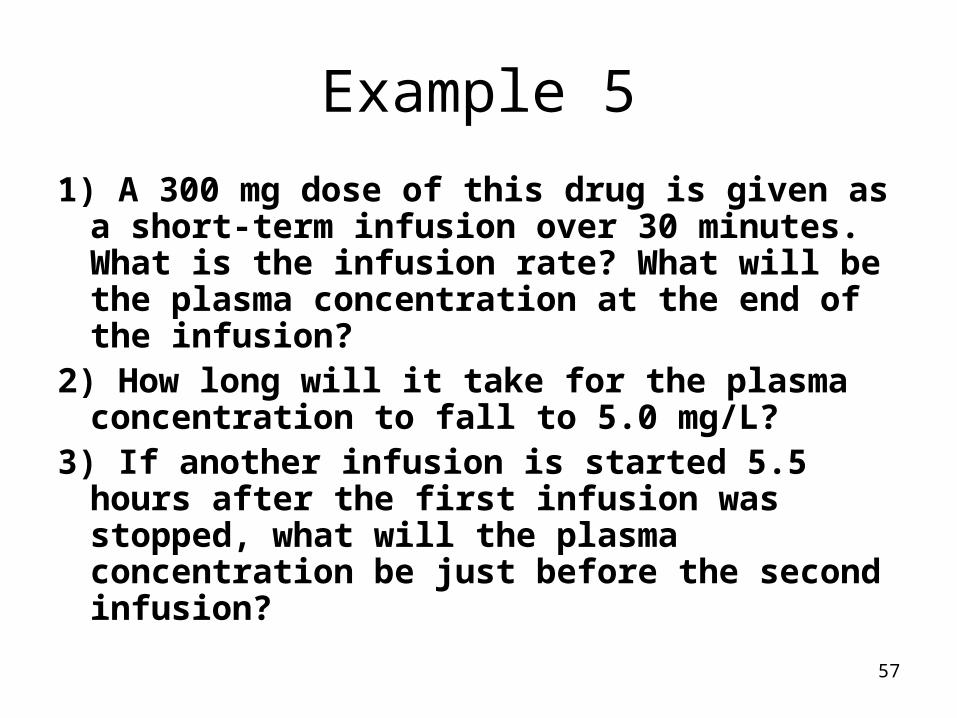
Example 5

1) A 300 mg dose of this drug is given as a short-term infusion over 30 minutes. What is the infusion rate? What will be the plasma concentration at the end of the infusion?

2) How long will it take for the plasma concentration to fall to 5.0 mg/L?

3) If another infusion is started 5.5 hours after the first infusion was stopped, what will the plasma concentration be just before the second infusion?

58

Example 5

1 (The infusion rate (K0) = Dose/duration = 300 mg/0.5 hr = 600 mg/hr.

Plasma concentration at the end of the infusion:

Infusion phase:

mg/L 71.9)1(L) 28)(hr 4.0(

mg/hr 600hr) 5.0(

1C

)5.0)(4.0(1-

0P

etC

eVK

K

P

tK

D

59

Example 5

2) Post infusion phase:

The concentration will fall to 5.0 mg/L 1.66 hr after the infusion was stopped.

hr 1.660.4

ln(5)ln(9.71)

K

)ln(C-infusion)) of end (at theln(Ct

tK-infusion)) of end (at theln(C)ln(C

einfusion) of end (at theCC

PP2

2PP

tkPP

2

60

Example 5

3) Post infusion phase (conc 5.5 hrs after stopping the infusion):

mg/L 08.19.71)e(hr) 5.5(tC

einfusion) of end (at theCC-.4)(5.5)(-0

p

tkPP

2

61

1 Laplace transformation. 2 The Laplace transform is a mathematical technique used for solving linear differential equations (apparent zero order and.

Documents