1 Introduction. 2 What is an Operating System? A program that acts as an intermediary between a user of a computer and the computer hardware. Operating.

1

Introduction

2

What is an Operating System?• A program that acts as an intermediary

between a user of a computer and the computer hardware.

• Operating system goals:– Execute user programs and make solving

user problems easier.– Make the computer system convenient to

use.

• Use the computer hardware in an efficient manner.

3

Computer System Components1. Hardware – provides basic computing resources

(CPU, memory, I/O devices).

2. Operating system – controls and coordinates the use of the hardware among the various application programs for the various users.

3. Applications programs – define the ways in which the system resources are used to solve the computing problems of the users (compilers, database systems, video games, business programs).

4. Users (people, machines, other computers).

4

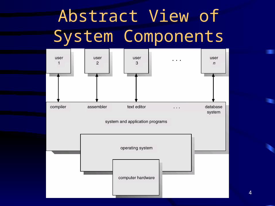
Abstract View of System Components

5

Computer-System Structures

6

Computer-System Architecture

7

Computer-System Operation• I/O devices and the CPU can execute

concurrently.• Each device controller is in charge of a particular

device type.• Each device controller has a local buffer.• CPU moves data from/to main memory to/from

local buffers• I/O is from the device to local buffer of controller.• Device controller informs CPU that it has finished

its operation by causing an interrupt.

8

Common Functions of Interrupts• Interrupts transfers control to the interrupt service

routine generally, through the interrupt vector, which contains the addresses of all the service routines.

• Interrupt architecture must save the address of the interrupted instruction.

• Incoming interrupts are disabled while another interrupt is being processed to prevent a lost interrupt.

• A trap is a software-generated interrupt caused either by an error or a user request.

• An operating system is interrupt driven.

9

Interrupt Handling• The operating system preserves the state of

the CPU by storing registers and the program counter.

• Determines which type of interrupt has occurred:– polling– vectored interrupt system

• Separate segments of code determine what action should be taken for each type of interrupt

10

Storage Structure• Main memory – only large storage media that the

CPU can access directly.• Secondary storage – extension of main memory

that provides large nonvolatile storage capacity.• Magnetic disks – rigid metal or glass platters

covered with magnetic recording material – Disk surface is logically divided into tracks, which are

subdivided into sectors.

– The disk controller determines the logical interaction between the device and the computer.

11

Moving-Head Disk Mechanism

12

Storage Hierarchy• Storage systems organized in hierarchy.

– Speed– cost– volatility

• Caching – copying information into faster storage system; main memory can be viewed as a last cache for secondary storage.

13

Storage-Device Hierarchy

14

Hardware Protection

• Dual-Mode Operation

• I/O Protection

• Memory Protection

• CPU Protection

15

Dual-Mode Operation• Sharing system resources requires operating

system to ensure that an incorrect program cannot cause other programs to execute incorrectly.

• Provide hardware support to differentiate between at least two modes of operations.1.User mode – execution done on behalf of a

user.

2.Monitor mode (also supervisor mode or system mode) – execution done on behalf of operating system.

16

Dual-Mode Operation (Cont.)• Mode bit added to computer hardware to

indicate the current mode: monitor (0) or user (1).

• When an interrupt or fault occurs hardware switches to monitor mode.

Privileged instructions can be issued only in monitor mode.

monitor user

Interrupt/fault

set user mode

17

I/O Protection• All I/O instructions are privileged

instructions.

• Must ensure that a user program could never gain control of the computer in monitor mode (I.e., a user program that, as part of its execution, stores a new address in the interrupt vector).

18

Processes

19

Process Concept• An operating system executes a variety of programs:

– Batch system – jobs

– Time-shared systems – user programs or tasks

• Textbook uses the terms job and process almost interchangeably.

• Process – a program in execution; process execution must progress in sequential fashion.

• A process includes:– program counter

– stack

– data section

20

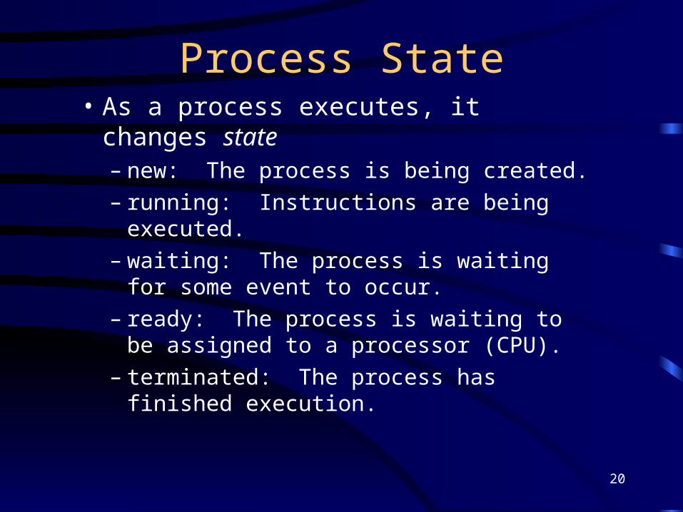
Process State• As a process executes, it changes state

– new: The process is being created.– running: Instructions are being executed.– waiting: The process is waiting for some

event to occur.– ready: The process is waiting to be

assigned to a processor (CPU).– terminated: The process has finished

execution.

21

Diagram of Process State

22

Process Control Block (PCB)Information associated with each process.• Process state - running, ready, etc.

• Program counter

• CPU registers• CPU scheduling information - process priority

• Memory-management information - location of page tables, limit registers

• Accounting information - CPU time used, etc.

• I/O status information - I/O devices allocated to process, list of open files

23

Process Control Block (PCB)

24

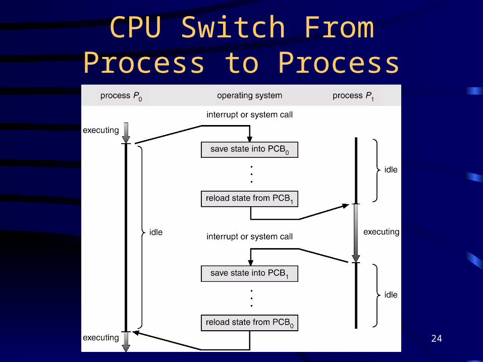
CPU Switch From Process to Process

25

Process Scheduling Queues

• Job queue – set of all processes in the system.• Ready queue – set of all processes residing in main memory,

ready and waiting to execute.• Device queues – set of processes waiting for an I/O device.• Process migration between the various queues.

26

Ready Queue And Various I/O Device Queues

27

Representation of Process Scheduling

28

Schedulers

• Long-term scheduler (or job scheduler) – selects which processes should be brought into the ready queue.

• Short-term scheduler (or CPU scheduler) – selects which process should be executed next and allocates CPU.

29

Addition of Medium Term Scheduling

30

Schedulers (Cont.)• Short-term scheduler is invoked very frequently

(milliseconds) (must be fast).

• Long-term scheduler is invoked very infrequently (seconds, minutes) (may be slow).

• The long-term scheduler controls the degree of multiprogramming.

• Processes can be described as either:– I/O-bound process – spends more time doing I/O than

computations, many short CPU bursts.

– CPU-bound process – spends more time doing computations; few very long CPU bursts.

31

Context Switch• When CPU switches to another process, the

system must save the state of the old process and load the saved state for the new process.

• Context-switch time is overhead; the system does no useful work while switching.

• Time dependent on hardware support.

32

CPU Processing

33

Basic Concepts

• Maximum CPU utilization obtained with multiprogramming

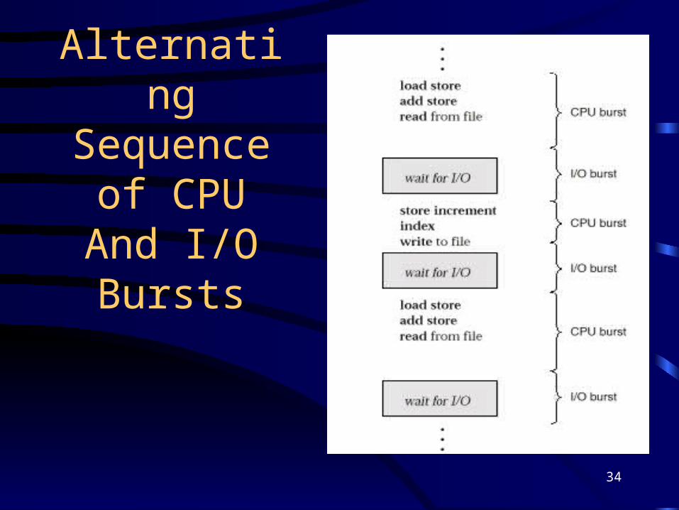
• CPU–I/O Burst Cycle – Process execution consists of a cycle of CPU execution and I/O wait.

• CPU burst distribution

34

Alternating Sequence of

CPU And I/O Bursts

35

Histogram of CPU-burst Times

36

CPU Scheduler• Selects from among the processes in memory that

are ready to execute, and allocates the CPU to one of them.

• CPU scheduling decisions may take place when a process:1. Switches from running to waiting state.

2. Switches from running to ready state.

3. Switches from waiting to ready.

4. Terminates.

37

Dispatcher• Dispatcher module gives control of the CPU

to the process selected by the short-term scheduler; this involves:– switching context– switching to user mode– jumping to the proper location in the user

program to restart that program

• Dispatch latency – time it takes for the dispatcher to stop one process and start another running.

38

Scheduling Criteria• CPU utilization – keep the CPU as busy

as possible• Throughput – # of processes that

complete their execution per time unit• Turnaround time – amount of time to

execute a particular process• Waiting time – amount of time a process

has been waiting in the ready queue

39

Scheduling Criteria• Response time – amount of time it

takes from when a request was submitted until the first response is produced, not output (for time-sharing environment)

40

Optimization Criteria

• Max CPU utilization

• Max throughput

• Min turnaround time

• Min waiting time

• Min response time

41

First-Come, First-Served (FCFS) Scheduling

• Example: Process Burst Time

P1 24

P2 3

P3 3

• The processes arrive in the order: P1 , P2 , P3

The Gantt Chart for the schedule is:

• Waiting time for P1 = 0; P2 = 24; P3 = 27

• Average waiting time: (0 + 24 + 27)/3 = 17

P1 P2 P3

24 27 300

42

FCFS Scheduling (Cont.)Suppose that the processes arrive in the order

P2 , P3 , P1 .

• The Gantt chart for the schedule is:

• Waiting time for P1 = 6; P2 = 0; P3 = 3

• Average waiting time: (6 + 0 + 3)/3 = 3• Much better than previous case.• Convoy effect short process behind long process

P1P3P2

63 300

43

Shortest-Job-First (SJR) Scheduling

• Associate with each process the length of its next CPU burst. Use these lengths to schedule the process with the shortest time.

44

Shortest-Job-First (SJR) Scheduling

• Two schemes: – nonpreemptive – once CPU given to the

process it cannot be preempted until completes its CPU burst.

– Preemptive – if a new process arrives with CPU burst length less than remaining time of current executing process, preempt. This scheme is know as the Shortest-Remaining-Time-First (SRTF).

• SJF is optimal – gives minimum average waiting time for a given set of processes.

45

Priority Scheduling

• A priority number (integer) is associated with each process

• The CPU is allocated to the process with the highest priority (smallest integer highest priority).– Preemptive– nonpreemptive

46

Priority Scheduling

• SJF is a priority scheduling where priority is the predicted next CPU burst time.

• Problem Starvation – low priority processes may never execute.

• Solution Aging – as time progresses increase the priority of the process.

47

Round Robin (RR)• Each process gets a small unit of CPU time

(time quantum), usually 10-100 milliseconds. After this time has elapsed, the process is preempted and added to the end of the ready queue.

• If there are n processes in the ready queue and the time quantum is q, then each process gets 1/n of the CPU time in chunks of at most q time units at once. No process waits more than (n-1)q time units.

48

Round Robin (RR)• Performance

– q large FIFO– q small q must be large with respect to

context switch, otherwise overhead is too high.

49

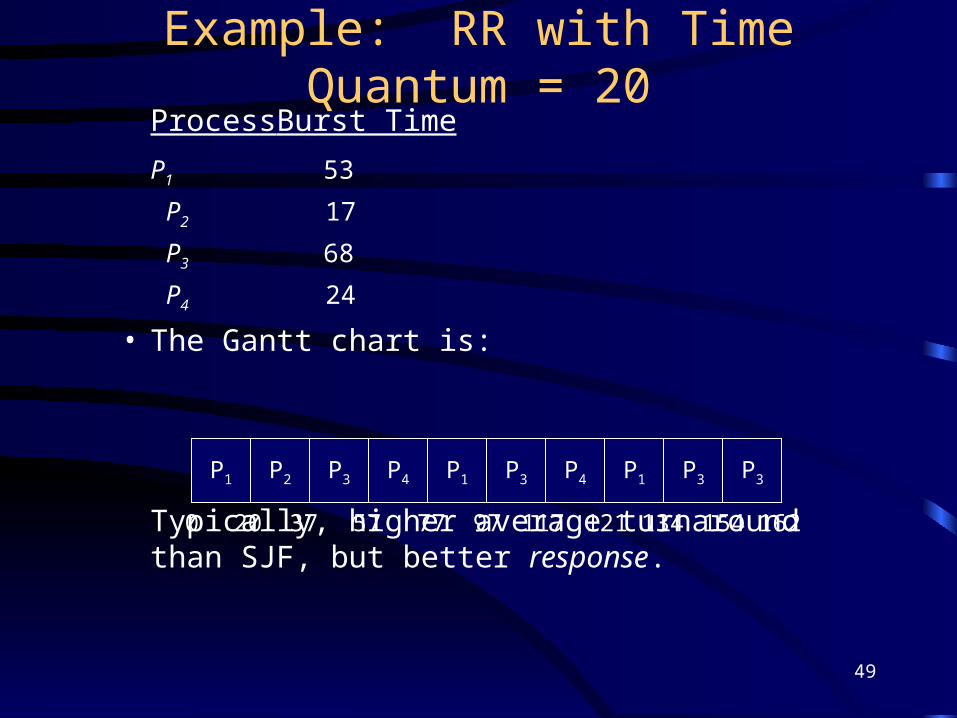
Example: RR with Time Quantum = 20Process Burst Time

P1 53

P2 17

P3 68

P4 24

• The Gantt chart is:

Typically, higher average turnaround than SJF, but better response.

P1 P2 P3 P4 P1 P3 P4 P1 P3 P3

0 20 37 57 77 97 117 121 134 154 162

50

Memory Management

51

Background• Program must be brought into memory and

placed within a process for it to be executed.

• Input queue – collection of processes on the disk that are waiting to be brought into memory for execution.

• User programs go through several steps before being executed.

52

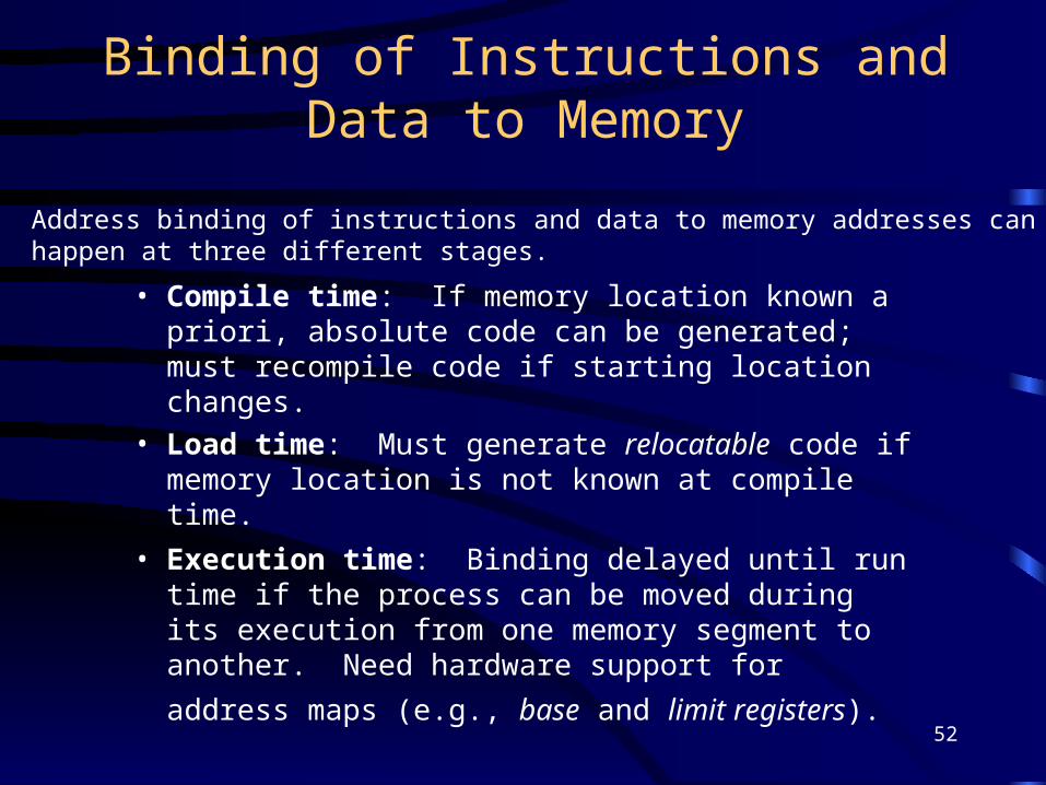
Binding of Instructions and Data to Memory

• Compile time: If memory location known a priori, absolute code can be generated; must recompile code if starting location changes.

• Load time: Must generate relocatable code if memory location is not known at compile time.

• Execution time: Binding delayed until run time if the process can be moved during its execution from one memory segment to another. Need hardware support for address maps (e.g., base and limit

registers).

Address binding of instructions and data to memory addresses canhappen at three different stages.

53

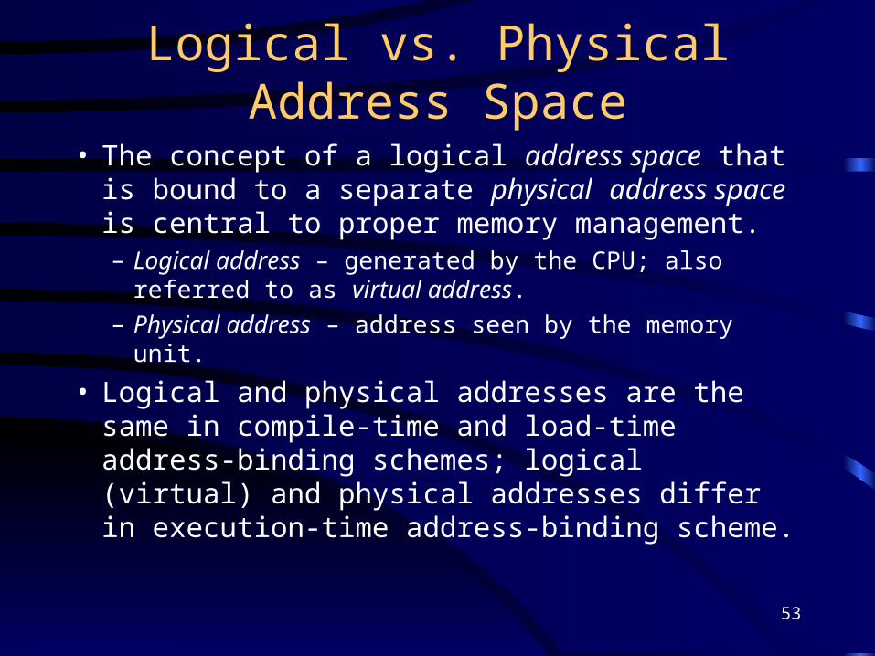
Logical vs. Physical Address Space

• The concept of a logical address space that is bound to a separate physical address space is central to proper memory management.– Logical address – generated by the CPU; also referred

to as virtual address.

– Physical address – address seen by the memory unit.

• Logical and physical addresses are the same in compile-time and load-time address-binding schemes; logical (virtual) and physical addresses differ in execution-time address-binding scheme.

54

Memory-Management Unit (MMU)

• Hardware device that maps virtual to physical address.

• In MMU scheme, the value in the relocation register is added to every address generated by a user process at the time it is sent to memory.

• The user program deals with logical addresses; it never sees the real physical addresses.

55

Contiguous Allocation• Main memory usually into two partitions:

– Resident operating system, usually held in low memory with interrupt vector.

– User processes then held in high memory.

• Single-partition allocation– Relocation-register scheme used to protect user

processes from each other, and from changing operating-system code and data.

– Relocation register contains value of smallest physical address; limit register contains range of logical addresses – each logical address must be less than the limit register.

56

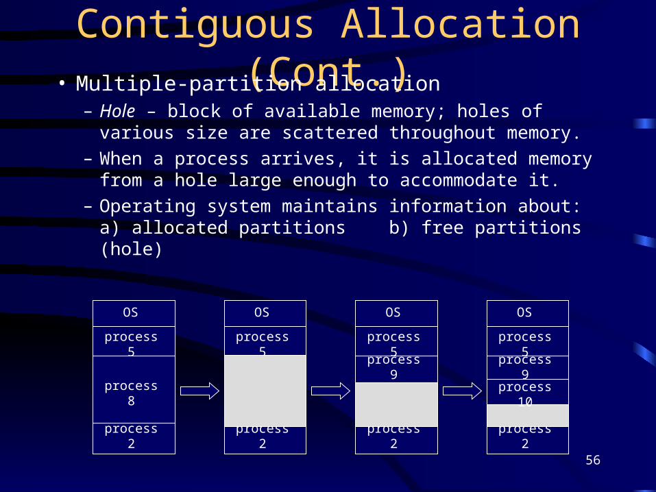
Contiguous Allocation (Cont.)• Multiple-partition allocation

– Hole – block of available memory; holes of various size are scattered throughout memory.

– When a process arrives, it is allocated memory from a hole large enough to accommodate it.

– Operating system maintains information about:a) allocated partitions b) free partitions (hole)

OS

process 5

process 8

process 2

OS

process 5

process 2

OS

process 5

process 2

OS

process 5

process 9

process 2

process 9

process 10

57

Dynamic Storage-Allocation Problem

• First-fit: Allocate the first hole that is big enough.

• Best-fit: Allocate the smallest hole that is big enough; must search entire list, unless ordered by size. Produces the smallest leftover hole.

• Worst-fit: Allocate the largest hole; must also search entier list. Produces the largest leftover hole.

How to satisfy a request of size n from a list of free holes.

First-fit and best-fit better than worst-fit in terms of speed and storage utilization.

58

Fragmentation• External fragmentation – total memory space

exists to satisfy a request, but it is not contiguous.• Internal fragmentation – allocated memory may be

slightly larger than requested memory; this size difference is memory internal to a partition, but not being used.

59

Fragmentation• Reduce external fragmentation by compaction

– Shuffle memory contents to place all free memory together in one large block.

– Compaction is possible only if relocation is dynamic, and is done at execution time.

– I/O problem• Latch job in memory while it is involved in I/O.

• Do I/O only into OS buffers.

60

Paging• Logical address space of a process can be

noncontiguous; process is allocated physical memory whenever the latter is available.

• Divide physical memory into fixed-sized blocks called frames (size is power of 2, between 512 bytes and 8192 bytes).

• Divide logical memory into blocks of same size called pages.

61

Paging• Keep track of all free frames.

• To run a program of size n pages, need to find n free frames and load program.

• Set up a page table to translate logical to physical addresses.

• Internal fragmentation.

62

Address Translation Scheme• Address generated by CPU is divided into:

– Page number (p) – used as an index into a page table which contains base address of each page in physical memory.

– Page offset (d) – combined with base address to define the physical memory address that is sent to the memory unit.

63

Address Translation Architecture

64

Paging Example

65

Implementation of Page Table• Page table is kept in main memory.• Page-table base register (PTBR) points to the page

table.• Page-table length register (PRLR) indicates size of

the page table.• In this scheme every data/instruction access requires

two memory accesses. One for the page table and one for the data/instruction.

• The two memory access problem can be solved by the use of a special fast-lookup hardware cache called associative registers or translation look-aside buffers (TLBs)

66

Associative Register• Associative registers – parallel search

• Address translation (A´, A´´)– If A´ is in associative register, get frame # out.

– Otherwise get frame # from page table in memory

Page # Frame #

67

Segmentation• Memory-management scheme that supports user view

of memory. • A program is a collection of segments. A segment is a

logical unit such as:

main program,

procedure,

function,

local variables, global variables,

common block,

stack,

symbol table, arrays

68

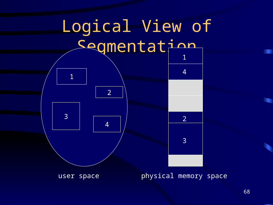
Logical View of Segmentation

1

3

2

4

1

4

2

3

user space physical memory space

69

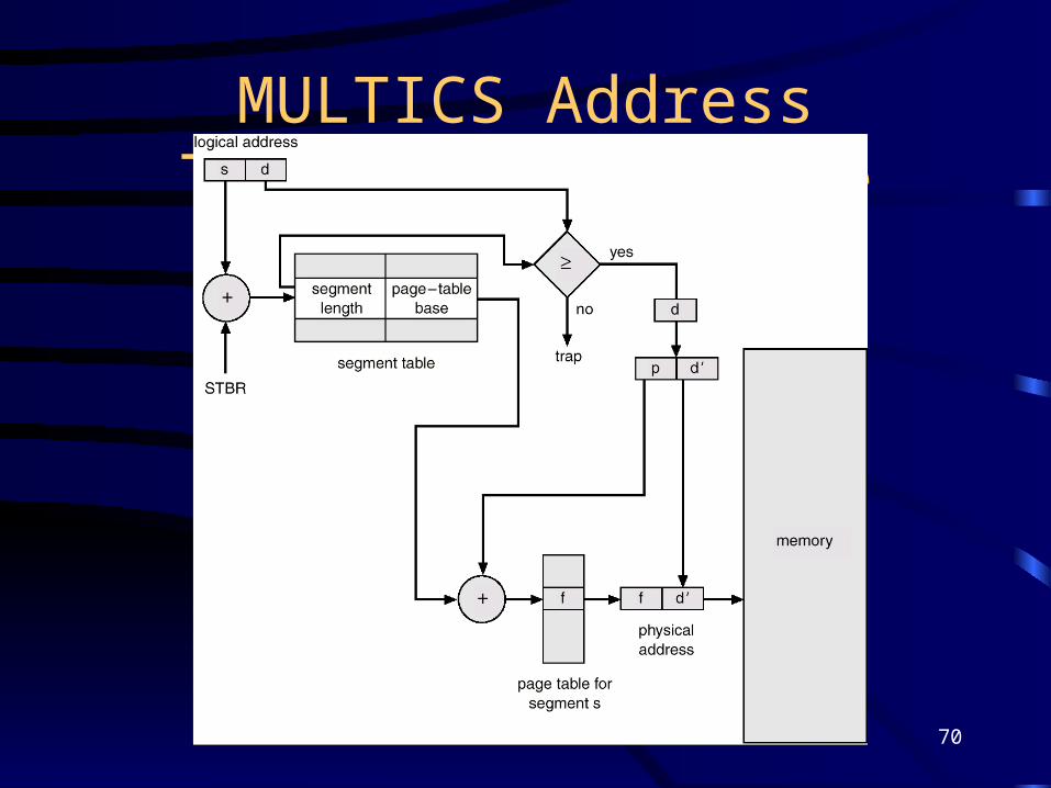
Segmentation Architecture • Logical address consists of a two tuple:

<segment-number, offset>,• Segment table – maps two-dimensional physical

addresses; each table entry has:– base – contains the starting physical address where the

segments reside in memory.– limit – specifies the length of the segment.

• Segment-table base register (STBR) points to the segment table’s location in memory.

• Segment-table length register (STLR) indicates number of segments used by a program;

segment number s is legal if s < STLR.

70

MULTICS Address Translation Scheme

71

Virtual Memory

72

Background• Virtual memory – separation of user logical

memory from physical memory.– Only part of the program needs to be in

memory for execution.– Logical address space can therefore be much

larger than physical address space.– Need to allow pages to be swapped in and out.

• Virtual memory can be implemented via:– Demand paging – Demand segmentation

73

Demand Paging• Bring a page into memory only when it is

needed.– Less I/O needed– Less memory needed – Faster response– More users

• Page is needed reference to it– invalid reference abort– not-in-memory bring to memory

74

Valid-Invalid Bit• With each page table entry a valid–invalid bit is

associated(1 in-memory, 0 not-in-memory)

• Initially valid–invalid but is set to 0 on all entries.

• During address translation, if valid–invalid bit in page table entry is 0 page fault.

111

1

0

00

Frame # valid-invalid bit

page table

75

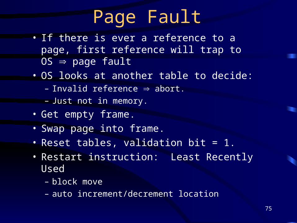
Page Fault• If there is ever a reference to a page, first

reference will trap to OS page fault

• OS looks at another table to decide:– Invalid reference abort.

– Just not in memory.

• Get empty frame.• Swap page into frame.• Reset tables, validation bit = 1.• Restart instruction: Least Recently Used

– block move

– auto increment/decrement location

76

What happens if there is no free frame?

• Page replacement – find some page in memory, but not really in use, swap it out.– algorithm– performance – want an algorithm which will

result in minimum number of page faults.

• Same page may be brought into memory several times.

77

Page Replacement• Prevent over-allocation of memory by

modifying page-fault service routine to include page replacement.

• Use modify (dirty) bit to reduce overhead of page transfers – only modified pages are written to disk.

• Page replacement completes separation between logical memory and physical memory – large virtual memory can be provided on a smaller physical memory.

78

Page-Replacement Algorithms• Want lowest page-fault rate.

• Evaluate algorithm by running it on a particular string of memory references (reference string) and computing the number of page faults on that string.

• In all our examples, the reference string is

1, 2, 3, 4, 1, 2, 5, 1, 2, 3, 4, 5.

79

First-In-First-Out Algorithm• Reference string: 1, 2, 3, 4, 1, 2, 5, 1, 2, 3, 4, 5

• 3 frames (3 pages can be in memory at a time per process)

• 4 frames

1

2

3

1

2

3

4

1

2

5

3

4

9 page faults

1

2

3

1

2

3

5

1

2

4

5 10 page faults

44 3

80

Optimal Algorithm• Replace page that will not be used for longest

period of time.• 4 frames example

1, 2, 3, 4, 1, 2, 5, 1, 2, 3, 4, 5

How do you know this?• Used for measuring how well your algorithm

performs.

1

2

3

4

6 page faults

4 5

81

Least Recently Used Algorithm• Reference string: 1, 2, 3, 4, 1, 2, 5, 1, 2, 3, 4, 5

• Counter implementation

– Every page entry has a counter; every time page is referenced through this entry, copy the clock into the counter.

– When a page needs to be changed, look at the counters to determine which are to change.

1

2

3

5

4

4 3

5

82

LRU Algorithm (Cont.)

• Stack implementation – keep a stack of page numbers in a double link form:– Page referenced:

• move it to the top

• requires 6 pointers to be changed

– No search for replacement

83

LRU Approximation Algorithms• Reference bit

– With each page associate a bit, initially -= 0– When page is referenced bit set to 1.– Replace the one which is 0 (if one exists). We do not know

the order, however.• Second chance

– Need reference bit.– Clock replacement.– If page to be replaced (in clock order) has reference bit = 1.

then:• set reference bit 0.• leave page in memory.• replace next page (in clock order), subject to same rules.

84

Counting Algorithms• Keep a counter of the number of references

that have been made to each page.

• LFU Algorithm: replaces page with smallest count.

• MFU Algorithm: based on the argument that the page with the smallest count was probably just brought in and has yet to be used.

85

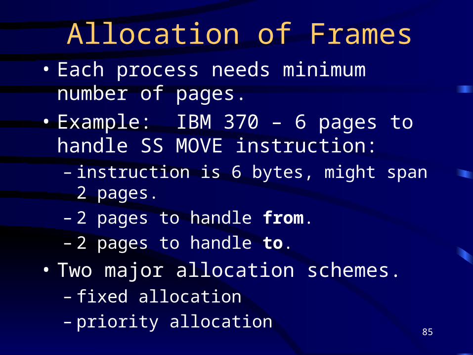
Allocation of Frames• Each process needs minimum number of

pages.

• Example: IBM 370 – 6 pages to handle SS MOVE instruction:– instruction is 6 bytes, might span 2 pages.– 2 pages to handle from.– 2 pages to handle to.

• Two major allocation schemes.– fixed allocation– priority allocation

86

Fixed Allocation

• Equal allocation – e.g., if 100 frames and 5 processes, give each 20 pages.

• Proportional allocation – Allocate according to the size of process.

87

Priority Allocation

• Use a proportional allocation scheme using priorities rather than size.

• If process Pi generates a page fault,

– select for replacement one of its frames.– select for replacement a frame from a process

with lower priority number.

88

Global vs. Local Allocation

• Global replacement – process selects a replacement frame from the set of all frames; one process can take a frame from another.

• Local replacement – each process selects from only its own set of allocated frames.

89

Thrashing• If a process does not have “enough” pages,

the page-fault rate is very high. This leads to:– low CPU utilization.– operating system thinks that it needs to increase

the degree of multiprogramming.– another process added to the system.

• Thrashing a process is busy swapping pages in and out.

90

Thrashing Diagram

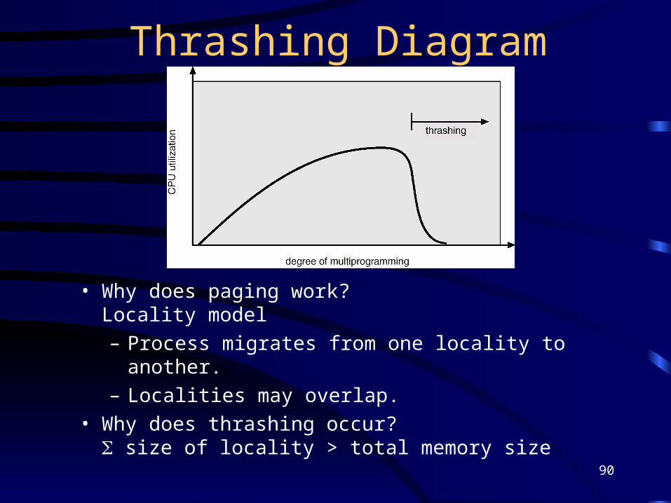
• Why does paging work?Locality model

– Process migrates from one locality to another.

– Localities may overlap.

• Why does thrashing occur? size of locality > total memory size

91

Working-Set Model working-set window a fixed number of page

references Example: 10,000 instruction

• WSSi (working set of Process Pi) =total number of pages referenced in the most recent (varies in time)

– if too small will not encompass entire locality.

– if too large will encompass several localities.

– if = will encompass entire program.

• D = WSSi total demand frames

• if D > m Thrashing

• Policy if D > m, then suspend one of the processes.