1. First of all we opened up a spreadsheet and started adding the data. 2. To work out the total cost for platinum, you times cell b5*c5 3. To calculate.

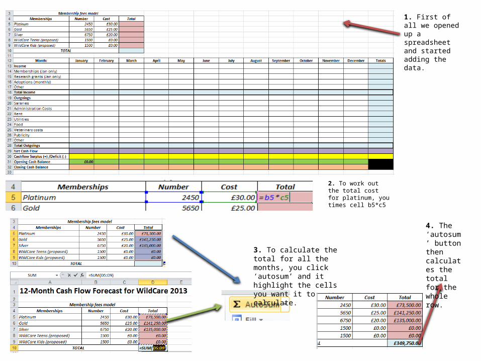
1. First of all we opened up a spreadsheet and started adding the data.

2. To work out the total cost for platinum, you times cell b5*c5

3. To calculate the total for all the months, you click ‘autosum’ and it highlight the cells you want it to calculate.

4. The ‘autosum’ button then calculates the total for the whole row.

Total Income1. To calculate the total income for each month you use a ‘SUM’ by adding a ‘=SUM’ equation it will calculate all the data in the cells that you want to add up.

2. This is the equation that should be present when calculating the total income for January. To do it for the rest of the months you follow the same process but different cells.

3. When you complete the total income for all the months this is what it looks like. When you start adding numbers in, it will add it up as it goes along, before calculating the total income.

Totals

4. You can also calculate the totals from January to February by using another ‘=SUM’ formula by adding the cells ‘B14:M14:’ after writing ‘SUM’ it will calculate the whole row.

Net Cash Flow

1. To calculate the ‘Net Cash Flow’ you add together the Total Income and the Total Outgoings which will give you the Net Cash Flow for each month.

2. To do this for all the months you can use another ‘=SUM’ formula to do all the months, or you can add all the months separately.

Net cash flow is the TOTAL INCOME-TOTAL OUTGOINGS which calculates how much money you have left.

Surplus and Deficit1. To calculate if the month was a ‘SURPLUS’ month which means the company gained a profit, or the company was ‘DEFICIT’ which means they lost money you would use this formula to complete it.

2. January was in DEFICIT as no money had gone into the company, and no money was gained, this is because we haven’t added the numbers yet.

3. I used the ‘=‘ to show it was a formula. The ‘IF’ part of it shows if it is an IF statement And I used the words “SURPLUS” , “DEFICIT” this would show up on the spreadsheet if it was a ‘SURPLUS’ month or a ‘DEFICIT’ one.

4. I used IF STATEMENTS to change what a cell says if it is in alliance with how much the Net Cash Flow was ( see above) I did this for each cell that needed them to have a “SURPLUS” or “DEFICIT” inputted into it.

Opening Cash Balance

1. Opening Cash Balance is the money left over from the month before, which is extra money added to the total at the end of the month, this is represented in the formula “=B32”

2. To calculate the Opening Cash Balance for each month, you can just use a formula using ‘=SUM’

Closing Cash Balance

3. The ‘closing cash balance’ is the money left at the end of the month, which can then get carried over to the next month for the ‘Opening Cash Flow’

4. To calculate the whole row, for all the months you would use a ‘=SUM’ formula this is easier and more efficient to calculating all the months, the formula would be “SUM=B31:M31”

Adding the numbers: Membership (Jan only)

1. To work out the Membership cost for January only you would use a formula, you would put an “=“ in cell B14, you would then click the cell “D10” for it to calculate the total amount of membership prices for January.

2. Due to this, this puts January into “SURPLUS” 3. You can then calculate the Memberships

column so the database is complete. It is easier and more efficient for every cell to be full, even if the total or cell is £0

Adding the numbers: Research Grants+Adoption costs

1. To calculate the total costs for January, you must click on the cell ‘B15’ and click ‘=‘ and then click the ‘costs’ page at the bottom of the spreadsheet and click on the ‘research grants’ section of the costs. Then click enter, this is the research grants for January.

2. After you click enter, it calculates the cost of the research grant for January and then calculates the ‘Total Income’ too.

Absolute Cell Referencing

Absolute Cell Referencing is very useful when you want a cell reference to stay fixed on a specific cell, meaning when a formula is copied and pasted to other cells, the cell references do not change at all. the cell reference "$B$24" is an absolute cell reference that always points to the cell in the first column and third row.

Cell FormattingCell formatting involves changing the format of cells, e.g from number to currency. This will make the spreadsheet easier to use, as it will be easy to tell which is which piece of data. It also means I can control the numbers of decimal points therefore controlling how accurate the data I input is.

Number Currency

3D Referencing3D Referencing allows you to insert or copy from one spread sheet to another easily. This is useful as it saves a lot of time and it means you can change the data on the original spreadsheet, and all the other data will change too, keeping the spreadsheet up to date. This is seen in my database below.

Formulae

Using formulas in Excel is very easy and very useful. It saves effort and time and means all the cells are connected as one and if one value changes so do all the others. This allows the database to keep up to date, or if I need to change anything.

IF Statements

IF Statements can be used if you want to see whether something is “TRUE” or “FALSE”. In this spreadsheet, I used an IF Statement to tell me if the values there were “Surplus” or “Deficit”, by seeing if one value was bigger than the other.

Goal Seek

Goal Seek is a series of commands, called what-if analysis (changing the values in cells to see how those changes affect the outcome of formulas) For example, varying the cells that is used in a table to determine the amount of the payments). When using goal seek (finding a specific value for a cell by changing the value of one other). Excel then varies the value in a cell that you specify until a formula that's dependent on that cell returns the result you want. I adjusted the ‘Membership Fees’ of all memberships to make the ‘Net Cash Flow’ as close to zero as possible.

Testing 1

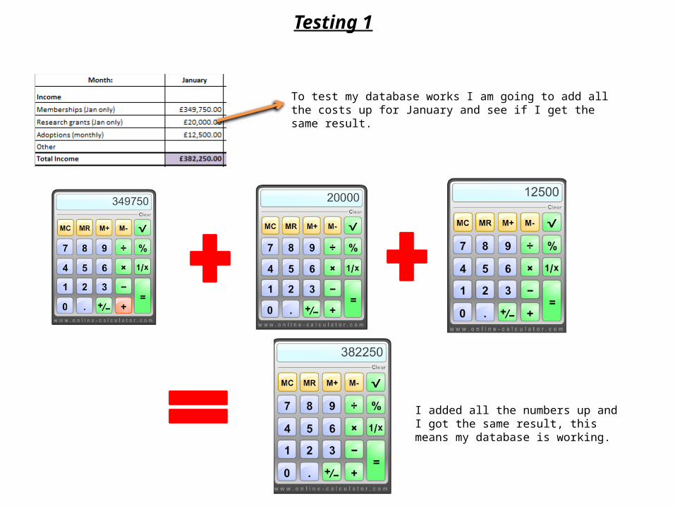
To test my database works I am going to add all the costs up for January and see if I get the same result.

I added all the numbers up and I got the same result, this means my database is working.

Testing 2

I added all the values together to make sure they all worked and added up to £57,301.00 and it did. The reason I tested and added all the numbers up is to make sure my database works properly.