Proceedings of 4th Jožef Stefan International Postgraduate School Students Conference Zbornik 4. Študentske konference Mednarodne podiplomske šole Jo žefa Stefana 25. maj 2012, Ljubljana, Slovenija Part 1. DEL

Welcome message from author
This document is posted to help you gain knowledge. Please leave a comment to let me know what you think about it! Share it to your friends and learn new things together.
Transcript

Proceedings of 4th Jožef Stefan International Postgraduate School Students ConferenceZbornik 4. Študentske konference Mednarodne podiplomske šole Jožefa Stefana
25. maj 2012, Ljubljana, Slovenija
Part 1. DEL
Zbornik 4. �tudentske konference Mednarodne podiplomske ²ole Joºefa Stefana(Proceedings of the 4th Joºef Stefan International Postgraduate School Students Conference)
Uredniki:Dejan PatelinAle² Tav£ar
Bo²tjan Kaluºa
Zaloºnik:Mednarodna podiplomska ²ola Joºefa Stefana, Ljubljana
Tisk:Franc Jagodic, s.p. - Jagraf
Naklada:150 izvodov
Ljubljana, maj 2012
IPSSC organizira ²tudentski svet Mednarodne podiplomske ²ole Joºefa �tefana(IPSSC is organized by Joºef Stefan International Postgraduate School - IPS student council)
CIP - Kataloºni zapis o publikacijiNarodna in univerzitetna knjiºnica, Ljubljana
5/6(082)378.046-021.68:001.891(497.4)(082)
MEDNARODNA podiplomska ²ola Joºefa Stefana. �tudentska konferenca (4 ; 2012 ; Ljubljana)Zbornik prispevkov = Proceedings / 4. ²tudentska konferenca
Mednarodne podiplomske ²ole Joºefa Stefana = 4th Joºef StefanInternational Postgraduate School Students Conference, 25. maj2012, Ljubljana, Slovenija ; [organizira ²tudentski svet Mednarodnepodiplomske ²ole Joºefa �tefana = organized by Joºef StefanInternational Postgraduate School - IPS Student Council] ; uredili,edited by Dejan Petelin, Ale² Tav£ar, Bo²tjan Kaluºa. - Ljubljana : Mednarodnapodiplomska ²ola Joºefa Stefana, 2012
ISBN 978-961-92871-4-91. Petelin, Dejan 2. Mednarodna podiplomska ²ola Joºefa Stefana (Ljubljana)
261775360
4. �TUDENTSKA KONFERENCA
MEDNARODNE PODIPLOMSKE �OLE
JO�EFA STEFANA
4th JO�EF STEFAN INTERNATIONAL POSTGRADUATE
SCHOOL STUDENTS CONFERENCE
Zbornik - 1. del
Proceedings - part 1
Uredili / Edited by
Dejan Petelin, Ale² Tav£ar in Bo²tjan Kaluºa
25. maj 2012, Ljubljana, Slovenija
Organizacijski odbor / Organising Committee
Dejan Petelin
Ale² Tav£ar
Bo²tjan Kaluºa
Hristjan Gjoreski
Piotr Sosnowski
Redakcijski odbor / Technical Review Committee
prof. dr. Gojmir Lahajnar
izr. prof. dr. Ester Heath
izr. prof. dr. Nives Ogrinc
izr. prof. dr. Jurij �ilc
Ana Miklav£i£
dr. Brigita Roºi£
Borut Sluban
Z inovativnimi raziskavami do tesnejšega sodelovanja z
gospodarstvom
Z lanskoletnim odličnim odzivom številnih uspešnih visokotehnoloških podjetij smo
dobili potrditev, da študentska konferenca napreduje in je vedno bolj zanimiva tako za
podjetja kot za študente. Tako smo se z velikim veseljem in zagonom ter v želji po
novih presežkih lotili organizacije že 4. študentske konference Mednarodne
podiplomske šole Jožefa Stefana, namenjene predstaviti naših raziskav širšemu
občinstvu in podjetjem ter s tem krepitvi povezav z gospodarstvom.
Ob začetku študijskega leta smo izdali knjižico s splošnim opisom študentske
konference, njenim namenom, dosedanjimi nagrajenci ter navodili za pripravo
prispevkov za sodelovanje na konferenci. Organizirali smo tudi sestanek z mentorji, na
katerem smo jim podrobno predstavili študentsko konferenco in poslanstvo le-te. Vse
te zgodnje priprave so se obrestovale, saj smo letos prejeli rekordnih 53 prispevkov. S
tem smo dobili tudi potrditev študentov, da se zavedajo pomembnosti konference in si
želijo sodelovanja s podjetji.
i

Pri tako številnih prispevkih smo želeli zagotoviti visoko kvaliteto le teh, zato smo v
letošnjem letu uvedli redakcijski odbor v sestavi sedmih članov. Vsak prispevek sta
temeljito pregledala dva člana odbora. Recenzenti so se poleg kakovosti prispevkov
osredotočali tudi na pravilnost in razumljivost besedila, še posebej splošnega povzetka,
ki je namenjen širšemu občinstvu, saj je le ta bistvenega pomena za razumevanje naših
raziskav s strani podjetij in s tem posledično vzpostavljanje stikov.
Za dodaten pretok informacij in vzpostavljanje stikov med študenti in podjetji smo
letos pripravili tudi okroglo mizo, na kateri sodelujejo tako predstavniki podjetij kot
predstavniki študentov. Pri tem si želimo, da bi se srečanje razvilo v aktivno razpravo,
ki bo zbližala poglede na povezovanje gospodarstva z raziskovalci tako predstavnikom
podjetij kot raziskovalcem in tako pripomogla k tesnejšemu in uspešnejšemu
sodelovanju.
Vsem študentom in njihovim mentorjem se zahvaljujemo za sodelovanje in s tem
izkazano zaupanje ter zavedanje pomembnosti sodelovanja z gospodarstvom. Zahvala
gre tudi vsem podjetjem, ki so kljub ne prav prijaznim časom za gospodarstvo
pokazala veliko mero razumevanja in želje po sodelovanju. Iskreno se jim
zahvaljujemo tako za finančno podporo, brez katere konference zagotovo ne bi uspeli
organizirati, kot za pripravljenost na sodelovanje. Predvsem pa se zahvaljujemo
celotnemu osebju na Mednarodni podiplomski šoli Jožefa Stefana za vso pomoč in
podporo. Še posebej gre velika zahvala dekanji prof. dr. Aleksandri Kornhauser
Frazer, ki ogromno prispeva tako k sami konferenci kot stalnemu napredku le te, ter
mag. Sergeji Vogrinčič, ki nam je pomagala prav pri vseh nalogah in težavah. Prav tako
se iskreno zahvaljujemo vsem članom redakcijskega odbora, ki so temeljito pregledali
vse prispevke in tako bistveno prispevali k še višji kvaliteti konference.
Uredniški odbor
ii

Beseda dekana MPŠ
V uvodu k prvi Študentski konferenci MPŠ je bila poudarjena želja, da bi te letne
prireditve postale tradicija šole. Zdaj – ob zaporedni četrti, doslej daleč največji –
čutimo, da se ta žlahtna tradicija uresničuje.
In taka tradicija je velika dragocenost, še posebej v svetu, ki ga pretresajo krize. Hude
krize so kot viharji – odnesejo vse, kar ni trdno ukoreninjeno. Tradicija, ki razvija
korenine, v takih dneh ni le obet za boljše pogoje, velikokrat je kar pogoj preživetja.
Mladi raziskovalci sprejemajo te konference kot svoj mladostno zagnani, a tudi že
samokritično izpostavljeni korak. Svoje začetne raziskovalne pobude, večkrat komaj
več kot sanje, v raziskovanju soočajo z eksperimentalnim preverjanjem in zahtevo o
ponovljivosti rezultatov. Predstavitev terja globlje razumevanje vpetosti rezultatov v
poznavanje sistemov in procesov. Zanesljivo se želi prepoznati njihov prispevek k
znanstvenim ugotovitvam, naj bo to trditvam ali dvomom.
V času, ko je gospodarsko preživetje razvitega sveta, še posebej Evrope, odvisno
predvsem od visokih tehnologij, se polagajo veliki upi na znanost. Ni več časa za
zaporedno postopnost v prenosu novega znanja v trajnostno razvijano proizvodnjo,
iii

Novi temeljni znanstveni dosežki se morajo sproti prenašati v razvojne procese.
Gospodarske organizacije, zlasti partnerji MPŠ, sodelujejo v pripravah in izvedbi teh
konferenc in tako omogočajo, da se svetova znanosti in gospodarstva vsaj na majhnih
področjih zlivata v celoto.
To nalaga mladim raziskovalcem in še posebej njihovim mentorjem tudi zahtevno skrb
za iskanje možnosti neposredne ali posredne uporabe raziskovalnih dosežkov za
razvoj proizvodnje in varovanje okolja. Znanstveno razmišljati pomeni danes celostno:
od porajanja originalnih zamisli in njihovega preverjanja in dopolnjevanja ter
poglabljanja znanja, preko oblikovanja novega znanja za prenos v uporabo, do izumov
in prek njih do inovacij. Te naj zvišujejo dodano vrednost, da bi lahko dvignili
kakovost življenja, ki bo omogočila tudi, da bi lahko še več in bolje raziskovali.
Da bi to dosegli, moramo spremeniti večkrat okostenelo miselnost, da je znanost
varna samo, če je povsem ločena od prakse. Naučiti se moramo tudi takega izražanja,
ki bo hkrati znanstveno dognano in širše razumljivo. Tak jezik ni le pogoj za najširše
možno razumevanje, je tudi bistveni del sodobne znanstvene kulture.
Čas je, da podiplomcem, ki predstavljajo svoje originalne zamisli ob vključevanju vseh
teh vidikov, ter njihovim mentorjem, ki jih spodbujajo in usmerjajo na tej strmi poti na
goro, ki se imenuje znanost, vsi čestitamo! Dolgujemo jim tudi zahvalo, da na
študentskih konferencah Mednarodne podiplomske šole Jožefa Stefana delijo z nami
svoje mladostne načrte, svoja iskanja, svoje dosežke in dvome ter zlasti svoja upanja,
da bodo kot raziskovalci prispevali k višji kakovosti življenja.
Prof. dr. Aleksandra Kornhauser Frazer
Dekan MPŠ
iv
Beseda predsednika MPŠ
Priča smo svetovni gospodarski recesiji, ki sovpada z ekonomsko krizo in krizo
družbenih vrednot, klimatskimi spremembami, problemi zdravja in zdrave prehrane,
pomanjkanja vode, ohranitve biodiverzitete in še kaj bi lahko dodali. Tej krizi so se v
dobri meri izognile države, ki so pravočasno zaznale te globalne probleme ter pričele
vlagati velika sredstva v znanost in raziskave, kot so npr. Nemčija, Skandinavske
države, Avstralija, Kitajska, Brazilija, Južna Afrika in še nekatere druge. Vse to delajo z
namenom, da bi zgradili kompetitivno, dinamično ter na znanju temelječo ekonomijo.
Osnova temu so odličnost v znanju, mednarodno povezovanje, hrabrost pri odločanju
ter svoboda. Vse naštete ekonomije so in še vedno zvišujejo finančna vlaganja v
znanost, ki je temelj inovacijam. V tej smeri deluje tudi vzpostavljeni Evropski
raziskovalni prostor – ERA, ki naj bi omogočal boljšo integracijo nacionalnih raziskav
v širšem evropskem prostoru ter s tem večjo konkurenčnost evropskega gospodarstva.
Vsako zaostajanje pomeni ekonomsko nestabilnost in izgubo samostojnosti.
Slovenija se je znašla v gospodarski recesiji. Za vrsto reševanja nakopičenih problemov
rabimo med drugim višja vlaganja v izobraževanje kvalitetnih kadrov. Še posebej
morajo biti napori usmerjeni v promocijo visokošolskega izobraževanja ter
raziskovalno dejavnost, kar omogoča in pospešuje zdravo tekmovalnost. Le to daje
v
odlične zaposlitvene možnosti, za kar je odgovornost deljena: politika, gospodarstvo,
univerze in raziskovalni instituti. To so izzivi za nove generacije, ki so upravičene do
boljše prihodnosti, kot jim jo ponuja sedanjost. Dolžni smo prihajajočim generacijam
omogočati, da se uspešno spopadejo z izzivi v domačem okolju, ne pa da iščejo
izpolnitve svojih ambicij in eksistenčnih možnosti z ''begom možganov'' v tujino.
S temi razmišljanji je Institut ''Jožef Stefan'' (IJS), najbolj elitna slovenska raziskovalna
organizacija na področju naravoslovnih in tehničnih ved, sprejel odločitev o
ustanovitvi Mednarodne podiplomske šole Jožefa Stefana (MPŠ). Po večletnih
prizadevanjih in s podporo uspešnih slovenskih gospodarskih podjetij je leta 2004
ustanovil samostojni visokošolski zavod. Študijske usmeritve zajemajo nova področja,
kot so nanotehnologije in nanoznanosti, informacijske in komunikacijske tehnologije,
ekotehnologije ter s tem povezan menedžment. Upravičenost ustanovitve te
podiplomske šole potrjuje dejstvo, da narašča zanimanje za študij. Tako je bilo v
šolskem letu 2011/2012 vpisanih 200 podiplomcev. Od ustanovitve šole pa do danes
je bilo podeljenih preko 90 doktoratov in 40 magisterijev.
IJS in MPŠ v tesni sodelavi izkoriščata odlično raziskovalno opremo vključno s Centri
odličnosti. Vrhunski kadrovski potenciali ter mednarodne povezave vključno s projekti
7. OP EU omogočajo usposabljanje na najvišji ravni ter prenašanje odličnega
sodobnega znanja, pridobljenega na temeljnih raziskavah, tudi v gospodarstvo. To je
misija naše Mednarodne podiplomske šole ter prispevek k pospešenemu zagonu
slovenskega gospodarstva ter hitrejšemu prehodu v družbo znanja.
Znanje je vrednota, ki omogoča narodu ekonomski razvoj in obstoj. Mladi vrhunski
raziskovalci, ki so pogoj za uspešen gospodarski razvoj, pa so srce družbe znanja.
Prof. dr. Vito Turk
Predsednik MPŠ
vi
Beseda predstavnice gospodarstva
Slovenska izvozno naravnana industrija se na globalnih trgih srečuje s svetovno
konkurenco. Za uvrščanje med vodilne ponudnike na ozkih programskih področjih
potrebuje vrhunske rešitve. Le-te pa lahko ustvarjajo samo razvojni timi v sodelovanju
z vztrajnimi, radovednimi raziskovalci z ambicijo, da se njihova dognanja iz
znanstvenih člankov prelijejo v iskane konkurenčne rešitve. Inovativnost, kreativnost,
znanje, pogum in vztrajnost v tekmi s konkurenco na svetovnih trgih so dejavniki, ki
omogočajo preboj v sam svetovni vrh. S prilagoditvijo vsebin podiplomskega
izobraževanja tudi raziskovalnim ciljem industrije, vključevanjem podiplomskih
študentov v mednarodne raziskovalne kroge in vrhunskim raziskovalnim okoljem na
IJS, se znanje pretvarja v izdelke z visoko dodano vrednostjo. Znanje omogoča
trajnostni razvoj podjetij ter posledično tudi nadaljnje raziskave. Raziskovalci MPŠ s
svojimi rezultati potrjujejo pravilnost vizionarske odločitve o ustanovitvi mednarodne
podiplomske šole.
dr. Jožica Rejec
Predsednica uprave Domel d.d.
vii

viii
Kazalo (Table of Contents)
Ekotehnologija (Ecotechnology) 1
The role of human activities on number concentration andsize distribution of particles in indoor airMateja Bezek, Janja Vaupoti£ 3
Cytostatics cyclophosphamide and ifosfamide � do theyoccur in Slovene wastewaters and surface waters?Marjeta �esen, Tina Kosjek, Ester Heath 9
Karakterizacija slovenskega olj£nega olja z uporabo stabil-nih izotopovMarinka Gams Petri²i£, Milena Bu£ar-Miklav£i£, Nives Ogrinc
15
Results of coal gas desorption experiments, laboratory sorp-tion experiments on lignite samples and in-situ seam gaspressure - rock stress measurementsSergej Jamnikar, Jerneja Lazar, Simon Zav²ek, Ludvik Golob 22
Jedkanje PET �lmov v poznem porazelektritvenem delukisikove plazmeMetod Kolar, Darij Kreuh, Alenka Vesel, Miran Mozeti£, KarinStana - Kleinschek 33
Entirely renewable and self-su�cient municipal energy sy-stemAnja Kostev²ek, Leon Cizelj, Janez Petek, Boris Su£i¢, MatevºPu²nik, Aleksandra Pivec 39
Selenium and its distribution in edible mussel Mytilus gal-loprovincialis collected from di�erent locationsUr²ka Kristan, Vekoslava Stibilj 45
Research of innovative technologies for degasi�cation of li-gnite seam
ix
Jerneja Lazar, Simon Zav²ek, Sergej Jamnikar, Janja �ula, Gre-gor Uranjek, Ludvik Golob 51
Use of monolithic chromatography for speciation of Pt ba-sed chemotherapeutic drugsAnºe Martin£i£, Radmila Mila£i£, Maja �emaºar, Gregor Ser²a,Janez �£an£ar 59
Determnation of Cr(VI) in corrosion protection coatings byspeciated isotope dilution ICP-MSBreda Novotnik, Tea Zuliani, Janez �£an£ar, Radmila Mila£i£ 65
Optimization of distillation separation procedure for me-thyl mercury in natural watersKristina Obu, Neºa Koron, Arne Bratki£, Mitja Vah£i£, MilenaHorvat 71
Photodegradation of BenzophenonesKristina Pestotnik, Tina Kosjek, Uro² Krajnc, Ester Heath 78
Poly[per�uorotitanate(IV)] Compounds of Alkali Metals,Unexpectedly Complicated Species in the Solid StateIgor Shlyapnikov, Evgeny Goreshnik, Zoran Mazej 84
Vibrational spectra calculation of triphenylene: compari-son of DFT and MP2 methodsGleb Veryasov, Dmitry Morozov, Ga²per Tav£ar 90
Hydrodynamic cavitation: a technique for augmentation ofremoval of persistent pharmaceuticals?Mojca Zupanc, Tina Kosjek, Boris Kompare, �eljko Blaºeka,Uro² Je²e, Matevº Dular, Brane �irok, Ester Heath 98
Informacijske in komunikacijske tehnologije (Infor-mation and Communication Technologies) 105
Reducing costs with computer power managementLucas Benedi£i£, Peter Koro²ec 107
x
Risk Assessment Using Local Outlier Factor AlgorithmBoºidara Cvetkovi¢, Mitja Lu²trek 113
Diagnostika sistemov z gorivnimi celicami in izbolj²anje nji-hovega delovanjaAndrej Debenjak 119
Risk Assessment Model for Congestive Heart FailureHristijan Gjoreski 125
Prototip sistema za sprotni nadzor stanja industrijske opremeMatic Ivanovi£, Ðani Juri£i¢ 131
Integration of structured expert knowledgeVladimir Kuzmanovski, Sa²o Dºeroski, Marko Debeljak 137
VESNA based platform for spectrum sensing in ISM bandsZoltan Padrah, Tomaº �olc, Mihael Mohor£i£ 144
Improving Performance of Wireless Mesh Networks withNetwork CodingErik Pertovt, Kemal Ali£, Ale² �vigelj, Mihael Mohor£i£ 150
Mobile terminal as opportunistic sensor network device forresearch on cognitive radio networksMarko Pesko, Luka Vidmar, Mitja �tular, Mihael Mohor£i£ 157
Inteligentni sistem za zaznavanje zdravstvenih teºav pristarej²ihBogdan Pogorelc 163
Sentiment analysis on tweets in a �nancial domainJasmina Smailovi¢, Miha Gr£ar, Martin �nidar²i£ 169
Cross-lingual named entity extraction and disambiguationTadej �tajner, Dunja Mladeni¢ 176
Extending the Multi-Criteria Decision Making Method DEXNejc Trdin, Marko Bohanec 182
xi
Development of Discovery and Identi�cation Protocol forSensor NetworksMatevº Vu£nik, Zoltan Padrah, Carolina Fortuna, Mihael Mo-hor£i£ 188
Nanoznanosti in nanotehnologije (Nanosciences andNanotechnologies) 195
Spectroscopic THz imaging using organic DSTMS (4-N,N-dimethylamino-4'-N'-methyl-stilbazolium 2,4,6-trimethyl-benzenesulfonate) crystalsAndreja Abina, Uro² Puc, David Heath, Aleksander Zidan²ek 197
In�uence of di�erent stress concentration factors in mono-leaf spring on its �nal fatigue lifePredrag Borkovi¢, Borivoj �u²tar²i£, Vojteh Leskov²ek, Borut�uºek 204
Tailoring electrically-induced properties by stretching re-laxor polymer �lmsG. Casar, A. Er²te, S. Glin²ek, X. Li, X. Qian, Q. M. Zhangand V. Bobnar 210
Terpolymer/copolymer blends on aluminum surface: Struc-tural, caloric, and dielectric propertiesAndreja Er²te, Vid Bobnar, Xian-Zhong Chen, Cheng-Liang Jia,Qun-Dong Shen 216
The adhesion of bacteria to austenitic stainless steel (AISI316L) with di�erent surface �nishesMatej Ho£evar, Monika Jenko, Damjana Drobne, Sara Novak 222
In�uence of the suspension stability on the deposition ofcobalt ferrite particles under an applied magnetic �eldPetra Jenu², Darja Lisjak, Darko Makovec, Miha Drofenik 228
Synthesis of cobalt ferrite nanoparticles using a combina-tion of the co-precipitation and hydrothermal methods
xii
Sonja Jovanovi¢, Matjaº Spreitzer, Mojca Otoni£ar, Danilo Su-vorov 234
Tempering E�ects on the Microstructure, Mechanical Pro-perties and Creep Rate of 20CrMoV121 and P91 SteelsFevzi Kafexhiu, Franc Vodopivec, Jelena Vojvodi£ � Tuma 241
Phase transitions of the NaNbO3 submicron-sized powderbetween room temperature and 700 ◦CJurij Koruza, Jenny Tellier, Barbara Mali£, Marija Kosec 247
Environmental Friendly Potassium Sodium Niobate BasedThin Films from SolutionsAlja Kupec, Barbara Mali£, Marija Kosec 254
The E�ect of the Firing Temperature on the Properties ofLTCCKostja Makarovi£, Anton Meden, Marko Hrovat, Janez Holc,Andreja Ben£an, Ale² Dakskobler, Darko Belavi£, Marija Kosec
261
Conformational preferences of alanine tripeptide in water,tri�uoroethanol and dimethyl sulfoxide studied by vi-brational spectroscopyAndreja Mirti£, Joºe Grdadolnik 268
Basic study of relaxors: Materials for high technologicaldevicesNikola Novak, Zdravko Kutnjak 275
Morfotropna fazna meja v (Na1−xKx)0,5Bi0,5TiO3 piezoelek-tri£ni keramikiMojca Otoni£ar 282
The peak base as a characteristic feature of the Auger elec-tron spectraBesnik Poniku, Igor Beli£, Monika Jenko 288
Underwater electromagnetic remote sensing
xiii
Uro² Puc, Andreja Abina, Anton Jegli£, Pavel Cevc, AleksanderZidan²ek 294
Estimating the size of the maximum inclusion in a largesample area of steelNu²a Puk²i£, Monika Jenko 301
Solvent capabilities of liquid and supercritical xenonKristian Radan, Boris �emva 307
A chemometric approach towards transmembrane regionprediction of protein sequencesAmrita Roy Choudhury, Marjana Novi£ 314
Vpliv legirnih elementov na lomno ºilavost vzmetnega jekla51CrV4Bojan Sen£i£, Vojteh Leskov²ek 320
Dielectric and ferroelectric properties of sol-gel-derivedNa0.5Bi0.5TiO3 thin �lmsTina �etinc, Matjaº Spreitzer, �pela Kunej, Danilo Suvorov 326
Synthesis and characterization of calcium phosphate coa-tings on ZrO2 ceramics for bone implant applicationsMartin �tefani£, Kristo�er Krnel, Tomaº Kosma£ 338
Photocatalytic discoloration of the azo dye methylene bluein the presence of irradiated TiO2/Pt nano-compositeVojka �uni£ 345
Life time assessment of real components exposed to hightemperatures and presuresBorut �uºek, Bojan Podgornik, Monika Jenko 354
xiv

Ekotehnologija (Ecotechnology)
1

The role of human activities on number concentration and size distribution of particles in indoor air
Mateja Bezek1,2, Janja Vaupotič1
1 Department of Environmental Sciences, Jožef Stefan Institute, Ljubljana, Slovenia
2 Jožef Stefan International Postgraduate School, Ljubljana, Slovenia
Abstract. Particle number concentrations and size distributions have been
monitored in the kitchen during candle burning and smoking a cigarette with a
Scanning Mobility Particle Sizer. Burning a candle produces particles in size range of
6–15 nm, whereas during smoking a cigarette, larger particles are formed in size
range of 40–150 nm. Total concentration of particles increased up to 1,341,000 and
423,000 cm–3 during burning a candle and smoking a cigarette, respectively.
Keywords: indoor air, nanoparticles, particle size distribution, total particle
concentration
1 Introduction
Particles are emitted in the atmosphere by a number of various human activities
[1, 2]. Important indoor particle sources in homes include cooking exhaust [3],
cigarette smoke [4], candles and other sorts of flames [2, 5] and solvents. At
workplaces many processes form particles, such as smelting, welding, soldering,
laser ablation, grinding and others[6]. Furthermore, huge amount of particles is
released to the atmosphere by biomass burning and traffic emissions [7].
Engineered nanoparticles are produced intentionally to be used in electronics,
medicines, pharmaceuticals, cosmetics, paints and a variety of other consumers’
products [8, 9].
Ultrafine particles (UFPs) or nanoparticles, defined as particles with aerodynamic
diameter <100 nm [10], are widely believed to be responsible for the adverse health
effects. During breathing of air, certain fraction of particles is deposited on the
walls of the respiratory tract. Strongly depending on the particle size, significant
3
amounts of particles are deposited in nasopharyngeal, traheobronhial and alveolar
region of respiratory tract [11]. Smaller particles are chemically and biochemically
more reactive and potentially more toxic than larger ones, due to large surface area.
With dropping particle size, the probability of deposition in respiratory system is
increasing [11, 12]. It has been recognised that nanoparticles cause oxidation stress,
pulmonary inflammation and cardiovascular events [11, 13]. Factors that influence
nanoparticle toxicity include size, number, surface characteristics, shape, chemical
composition, surface treatment and potential for agglomeration [14, 15].
In this paper characterization of particles formed during burning a candle and
smoking a cigarette is given. We have focused on fraction below 100 nm,
comparing fractions of particles below 20 and 10 nm, which are potentially more
toxic due to deeper penetration in respiratory tract.
2 Experimental
Indoor measurements were performed in the kitchen of the basement flat in the
suburb of Ljubljana during two experiments, burning a candle and smoking a
cigarette. Particle number concentrations and size distributions during these
experiments were measured with a Scanning Mobility Particle Sizer + Counter
(SMPS+C, Series 5.400, Grimm, Germany). Differential Mobility Analyzer (DMA)
unit separates charged particles into 44 channels based on their electrical mobility
(d), which depends on the particle size and electrical charge. Afterwards, in the
Condensation Particle Counter (CPC) they are enhanced and counted.
The frequency of measurement with medium DMA unit is one in four minutes for
size range 5–350 nm. The instrument gives the total number concentration of
particles C(tot), the geometric mean of their diameters dGM, and the number size
distribution. In addition, fractions of particles below 10, 20 and 100 nm (x(<10),
x(<20) and x(<100)) were calculated.
3 Results and Discussion
Particle size distributions during burning a candle and smoking a cigarette are
presented in Figure 1. During burning a candle (Figure 1a) high particle
4
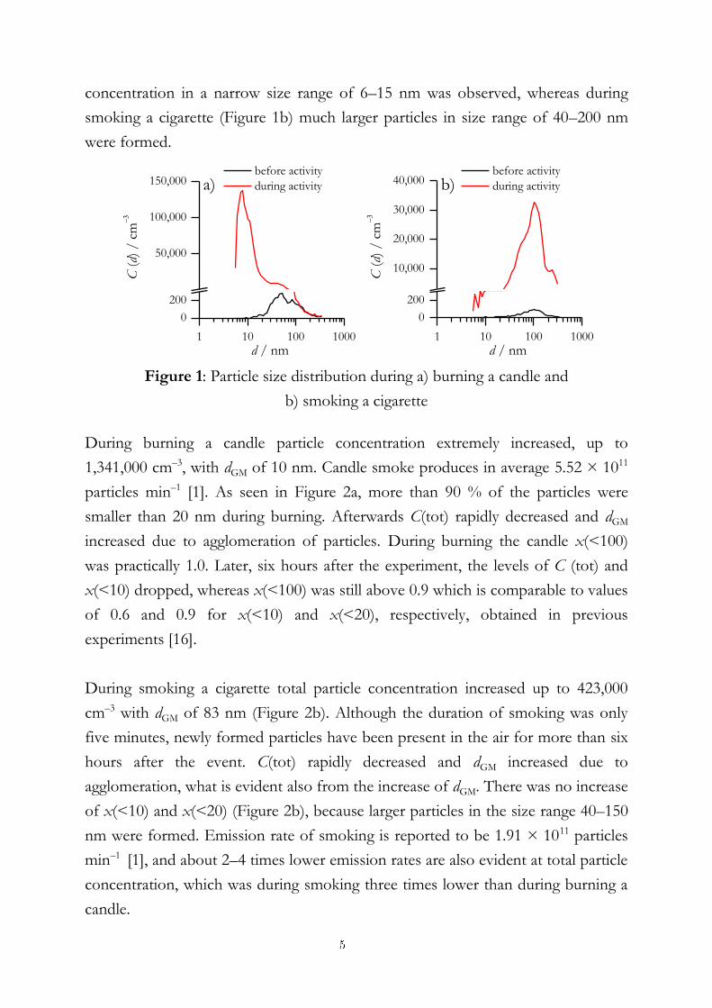
concentration in a narrow size range of 6–15 nm was observed, whereas during
smoking a cigarette (Figure 1b) much larger particles in size range of 40–200 nm
were formed.
1 10 100 1000
0
200
50,000
100,000
150,000 a)
C (
d) /
cm
d / nm
before activity
during activity
1 10 100 1000
0
200
10,000
20,000
30,000
40,000 b)
C (
d) /
cm
d / nm
before activity
during activity
Figure 1: Particle size distribution during a) burning a candle and
b) smoking a cigarette
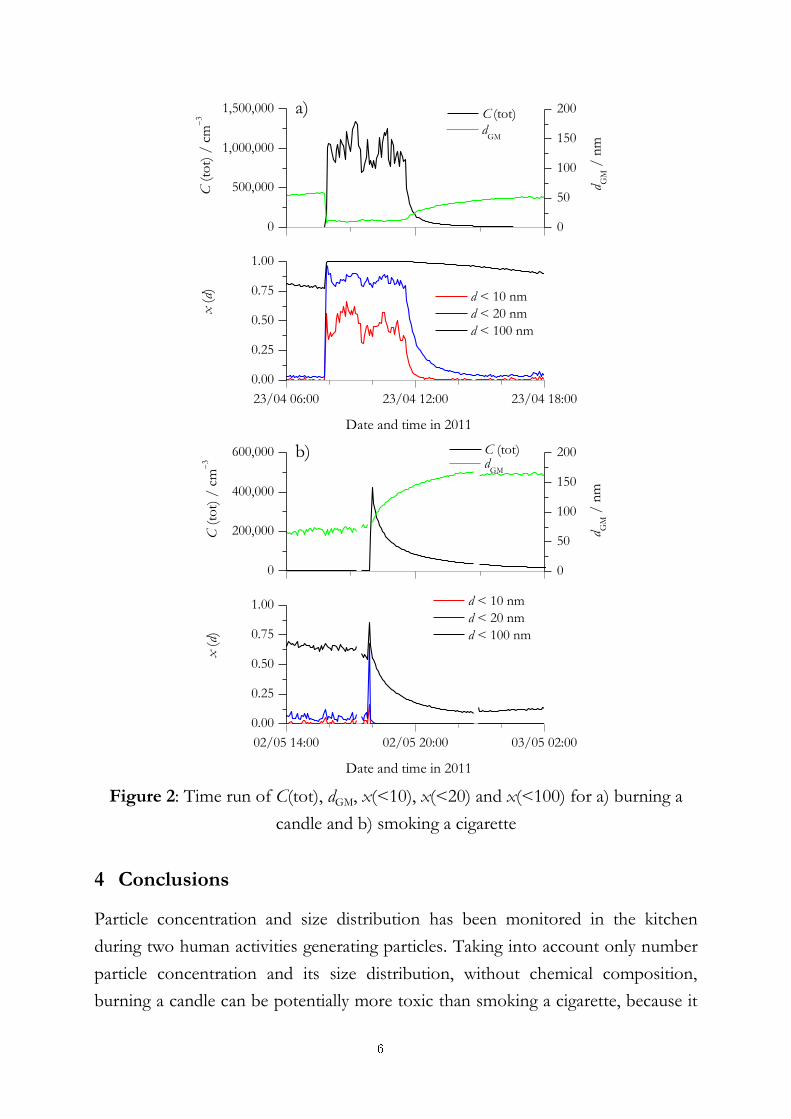
During burning a candle particle concentration extremely increased, up to
1,341,000 cm–3, with dGM of 10 nm. Candle smoke produces in average 5.52 × 10¹¹
particles min–1 [1]. As seen in Figure 2a, more than 90 % of the particles were
smaller than 20 nm during burning. Afterwards C(tot) rapidly decreased and dGM
increased due to agglomeration of particles. During burning the candle x(<100)
was practically 1.0. Later, six hours after the experiment, the levels of C (tot) and
x(<10) dropped, whereas x(<100) was still above 0.9 which is comparable to values
of 0.6 and 0.9 for x(<10) and x(<20), respectively, obtained in previous
experiments [16].
During smoking a cigarette total particle concentration increased up to 423,000
cm–3 with dGM of 83 nm (Figure 2b). Although the duration of smoking was only
five minutes, newly formed particles have been present in the air for more than six
hours after the event. C(tot) rapidly decreased and dGM increased due to
agglomeration, what is evident also from the increase of dGM. There was no increase
of x(<10) and x(<20) (Figure 2b), because larger particles in the size range 40–150
nm were formed. Emission rate of smoking is reported to be 1.91 × 10¹¹ particles
min–1 [1], and about 2–4 times lower emission rates are also evident at total particle
concentration, which was during smoking three times lower than during burning a
candle.
5
23/04 06:00 23/04 12:00 23/04 18:00
0.00
0.25
0.50
0.75
1.00
d < 10 nm
d < 20 nm
d < 100 nm
x (
d)
Date and time in 2011
a)
0
500,000
1,000,000
1,500,000
d GM
/ n
m
C (tot)
C (
tot)
/ c
m
3
0
50
100
150
200
dGM
02/05 14:00 02/05 20:00 03/05 02:00
0.00
0.25
0.50
0.75
1.00 d < 10 nm
d < 20 nm
d < 100 nm
x (
d)
Date and time in 2011
b)
0
200,000
400,000
600,000
d GM
/ n
m
C (tot)
C (
tot)
/ c
m
3
0
50
100
150
200 d
GM
Figure 2: Time run of C(tot), dGM, x(<10), x(<20) and x(<100) for a) burning a
candle and b) smoking a cigarette
4 Conclusions
Particle concentration and size distribution has been monitored in the kitchen
during two human activities generating particles. Taking into account only number
particle concentration and its size distribution, without chemical composition,
burning a candle can be potentially more toxic than smoking a cigarette, because it
6
produces significantly smaller particles and higher number concentration of
particles. Furthermore longer retention time of particles formed during burning a
candle in the air leads to longer exposure time. In our future work, analyses of
particle shape, morphology and chemical composition are foreseen.
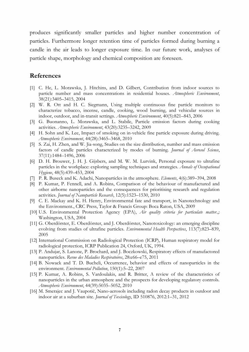
References
[1] C. He, L. Morawska, J. Hitchins, and D. Gilbert, Contribution from indoor sources to particle number and mass concentrations in residential houses. Atmospheric Environment, 38(21):3405–3415, 2004
[2] W. R. Ott and H. C. Siegmann, Using multiple continuous fine particle monitors to characterize tobacco, incense, candle, cooking, wood burning, and vehicular sources in indoor, outdoor, and in-transit settings. Atmospheric Environment, 40(5):821–843, 2006
[3] G. Buonanno, L. Morawska, and L. Stabile, Particle emission factors during cooking activities. Atmospheric Environment, 43(20):3235–3242, 2009
[4] H. Sohn and K. Lee, Impact of smoking on in-vehicle fine particle exposure during driving. Atmospheric Environment, 44(28):3465–3468, 2010
[5] S. Zai, H. Zhen, and W. Jia-song, Studies on the size distribution, number and mass emission factors of candle particles characterized by modes of burning. Journal of Aerosol Science, 37(11):1484–1496, 2006
[6] D. H. Brouwer, J. H. J. Gijsbers, and M. W. M. Lurvink, Personal exposure to ultrafine particles in the workplace: exploring sampling techniques and strategies. Annals of Occupational Hygiene, 48(5):439–453, 2004
[7] P. R. Buseck and K. Adachi, Nanoparticles in the atmosphere. Elements, 4(6):389–394, 2008 [8] P. Kumar, P. Fennell, and A. Robins, Comparison of the behaviour of manufactured and
other airborne nanoparticles and the consequences for prioritising research and regulation activities. Journal of Nanoparticle Research, 12(5):1523–1530, 2010
[9] C. E. Mackay and K. H. Henry, Environmental fate and transport, in Nanotechnology and the Environment., CRC Press, Taylor & Francis Group: Boca Raton, USA, 2009
[10] U.S. Environmental Protection Agency (EPA), Air quality criteria for particulate matter.,: Washington, USA, 2004
[11] G. Oberdörster, E. Oberdörster, and J. Oberdörster, Nanotoxicology: an emerging discipline evolving from studies of ultrafine particles. Environmental Health Perspectives, 113(7):823–839, 2005
[12] International Commission on Radiological Protection (ICRP), Human respiratory model for radiological protection, ICRP Publication 24, Oxford, UK, 1994.
[13] P. Andujar, S. Lanone, P. Brochard, and J. Boczkowski, Respiratory effects of manufactored nanoparticles. Revue des Maladies Respiratoires, 28:e66–e75, 2011
[14] B. Nowack and T. D. Bucheli, Occurrence, behavior and effects of nanoparticles in the environment. Environmental Pollution, 150(1):5–22, 2007
[15] P. Kumar, A. Robins, S. Vardoulakis, and R. Britter, A review of the characteristics of nanoparticles in the urban atmosphere and the prospects for developing regulatory controls. Atmospheric Environment, 44(39):5035–5052, 2010
[16] M. Smerajec and J. Vaupotič, Nano-aerosols including radon decay products in outdoor and indoor air at a suburban site. Journal of Toxicology, ID 510876, 2012:1–31, 2012
7
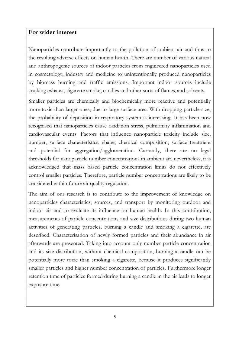
For wider interest
Nanoparticles contribute importantly to the pollution of ambient air and thus to
the resulting adverse effects on human health. There are number of various natural
and anthropogenic sources of indoor particles from engineered nanoparticles used
in cosmetology, industry and medicine to unintentionally produced nanoparticles
by biomass burning and traffic emissions. Important indoor sources include
cooking exhaust, cigarette smoke, candles and other sorts of flames, and solvents.
Smaller particles are chemically and biochemically more reactive and potentially
more toxic than larger ones, due to large surface area. With dropping particle size,
the probability of deposition in respiratory system is increasing. It has been now
recognised that nanoparticles cause oxidation stress, pulmonary inflammation and
cardiovascular events. Factors that influence nanoparticle toxicity include size,
number, surface characteristics, shape, chemical composition, surface treatment
and potential for aggregation/agglomeration. Currently, there are no legal
thresholds for nanoparticle number concentrations in ambient air, nevertheless, it is
acknowledged that mass based particle concentration limits do not effectively
control smaller particles. Therefore, particle number concentrations are likely to be
considered within future air quality regulation.
The aim of our research is to contribute to the improvement of knowledge on
nanoparticles characteristics, sources, and transport by monitoring outdoor and
indoor air and to evaluate its influence on human health. In this contribution,
measurements of particle concentrations and size distributions during two human
activities of generating particles, burning a candle and smoking a cigarette, are
described. Characterisation of newly formed particles and their abundance in air
afterwards are presented. Taking into account only number particle concentration
and its size distribution, without chemical composition, burning a candle can be
potentially more toxic than smoking a cigarette, because it produces significantly
smaller particles and higher number concentration of particles. Furthermore longer
retention time of particles formed during burning a candle in the air leads to longer
exposure time.
8
Cytostatics cyclophosphamide and ifosfamide – do they occur in Slovene wastewaters and surface waters?
Marjeta Česen1,2, Tina Kosjek1, Ester Heath1,2
1 Department of Environmental Sciences, Jožef Stefan Institute, Ljubljana, Slovenia
2 Jožef Stefan International Postgraduate School, Ljubljana, Slovenia
Abstract. To assess pollution of the Slovene aquatic environment by the
cytostatics cyclophosphamide (CF) and ifosfamide (IF), we developed an
analytical method for their analysis in wastewater and surface water by gas
chromatography-mass spectrometry (GC-MS). Samples were collected and
analyzed from the Institute of Oncology Ljubljana, the Central
Wastewater Treatment Plant in Ljubljana and from the Ljubljanica River
downstream from the WWTP discharge. Results revealed concentrations in
wastewater from the Institute of Oncology of 12.1 µg L-1 and 10.5 µg L-1 for
CF and IF, respectively. At other locations the concentrations of CF and IF
were under their detection limits. In the future the method will be further
optimized in order to detect lower concentrations of CF and IF. In addition,
the study will be extended to include wastewaters and surface waters from
other locations in Slovenia as well as the main metabolites of CF and IF.
Keywords: cyclophosphamide, ifosfamide, wastewater, Institute of Oncology
Ljubljana, Central Wastewater Treatment Plant Ljubljana, gas
chromatography-mass spectrometry
1 Introduction
Cyclophosphamide (CF) and ifosfamide (IF) are cytostatic compounds used in
chemotherapy to treat patients with cancer and certain autoimmune diseases
(Figure 1). Since their action is based on alkylation of nucleophilic compounds,
9
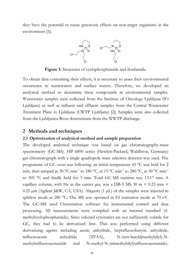
they have the potential to cause genotoxic effects on non-target organisms in the
environment [1].
Figure 1: Structures of cyclophosphamide and ifosfamide.
To obtain data concerning their effects, it is necessary to asses their environmental
occurrence in wastewaters and surface waters. Therefore, we developed an
analytical method to determine these compounds in environmental samples.
Wastewater samples were collected from the Institute of Oncology Ljubljana (IO
Ljubljana) as well as influent and effluent samples from the Central Wastewater
Treatment Plant in Ljubljana (CWTP Ljubljana) [2]. Samples were also collected
from the Ljubljanica River downstream from the WWTP discharge.
2 Methods and techniques
2.1 Optimization of analytical method and sample preparation
The developed analytical technique was based on gas chromatography-mass
spectrometry (GC-MS). HP 6890 series (Hewlett-Packard, Waldbron, Germany)
gas chromatograph with a single quadrupole mass selective detector was used. The
programme of GC oven was following: an initial temperature 65 °C was held for 2
min, then ramped at 30 °C min-1 to 180 °C, at 15 °C min-1 to 280 °C, at 30 °C min-1
to 305 °C and finally held for 3 min. Total GC-MS runtime was 13.17 min. A
capillary column, with He as the carrier gas, was a DB-5 MS 30 m × 0.25 mm ×
0.25 µm (Agilent J&W, CA, USA). Aliquots (1 µL) of the samples were injected in
splitless mode at 280 °C. The MS was operated in EI ionisation mode at 70 eV.
The GC-MS used Chemstation software for instrumental control and data
processing. All measurements were complied with an internal standard (4-
methylcyclophosphamide). Since selected cytostatics are not sufficiently volatile for
GC, they had to be derivatized first. This was performed using different
derivatizing agents including acetic anhydride, heptafluorobutyric anhydride,
trifluoroacetic anhydride (TFAA), N-(tert-butyldimethylsilyl)-N-
methyltrifluoroacetamide and N-methyl-N-(trimethylsilyl)trifluoroacetamide).
10
Different derivatization times and temperatures were also investigated. Optimal
derivatization was achieved by addition of 100 µL of TFAA to the sample, which
was then derivatized for 0.5 h at 60 °C. For extraction, HLB OasisTM cartridges
(3cc, 60 mg) were used. Cartridges were conditioned using 3 mL of ethyl acetate, 3
mL of methanol and 3 mL of tap water. Optimal elution was achieved with 3 mL
of ethyl acetate.
Grab samples were taken from the wastewater collection basin at IO Ljubljana and
at Ljubljanica River (downstream from the WWTP discharge). Time-proportional
samples (24 hours) were collected from the WWTP’s influent and effluent. All
samples were immediately transported on ice to the laboratory, where they were
filtered (0.45 µm cellulose nitrate filters) and stored at - 20°C until analysis.
2.2 Sample analysis
To estimate the concentration range of CF and IF, different volumes of the
samples were extracted and analyzed (200 mL, 500 mL and 1000 mL). For this
purpose we used wastewater influent from laboratory-scale biological treatment
plant (V = 200 mL). Recovery (%) was determined using 0.5 µgL-1 of CF and IF
and was calculated as ratio between peak areas of spiked amount of analyte, which
was added prior to extraction (n = 3), and peak areas of same amount of analyte,
added post extraction (n = 3). A six point calibration was performed (n = 3). Linear
regression was used to obtain the r2 values. LOD (limit of detection) and LOQ
(limit of quantification) were determined as 3-times (LOD) and 10-times (LOQ)
standard deviations of the peak areas of the baseline from the blanks (n = 6)
divided by the slope of calibration curve. Repeatability was calculated as RSD at
three concentration levels (500 ng L-1 , 5000 ng L-1 , 10000 ng L-1; n = 3)
3 Results and discussion
Optimal volume for analysis of wastewater from IO Ljubljana was 200 mL, while
samples of influent and effluent of CWTP Ljubljana and Ljubljanica River
contained undetectable concentrations of CF and IF at these volumes and specified
conditions of analytical method. The linear range, recoveries (%), LOD, LOQ, r2
values and repeatability (RSD values) for CF and IF are shown in Table 1.
11
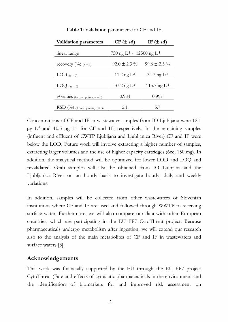
Table 1: Validation parameters for CF and IF.
Validation parameters CF (± sd) IF (± sd)
linear range 750 ng L-1 - 12500 ng L-1
(both)
recovery (%) (n = 3) 92.0 ± 2.3 % 99.6 ± 2.3 %
LOD (n = 6) 11.2 ng L-1 34.7 ng L-1
LOQ ( n = 6) 37.2 ng L-1 115.7 ng L-1
r2 values (6 conc. points, n = 3) 0.984 0.997
RSD (%) (3 conc. points, n = 3) 2.1 5.7
Concentrations of CF and IF in wastewater samples from IO Ljubljana were 12.1
µg L-1 and 10.5 µg L-1 for CF and IF, respectively. In the remaining samples
(influent and effluent of CWTP Ljubljana and Ljubljanica River) CF and IF were
below the LOD. Future work will involve extracting a higher number of samples,
extracting larger volumes and the use of higher capacity cartridges (6cc, 150 mg). In
addition, the analytical method will be optimized for lower LOD and LOQ and
revalidated. Grab samples will also be obtained from IO Ljubjana and the
Ljubljanica River on an hourly basis to investigate hourly, daily and weekly
variations.
In addition, samples will be collected from other wastewaters of Slovenian
institutions where CF and IF are used and followed through WWTP to receiving
surface water. Furthermore, we will also compare our data with other European
countries, which are participating in the EU FP7 CytoThreat project. Because
pharmaceuticals undergo metabolism after ingestion, we will extend our research
also to the analysis of the main metabolites of CF and IF in wastewaters and
surface waters [3].
Acknowledgements
This work was financially supported by the EU through the EU FP7 project
CytoThreat (Fate and effects of cytostatic pharmaceuticals in the environment and
the identification of biomarkers for and improved risk assessment on
12

environmental exposure, grant agreement No.: 265264) and by the Slovenian
Research Agency (Program Group P1-0143 and Young Researcher grant to M. Č.).
We would also like to thank IO Ljubljana and JP Vodovod-Kanalizacija d.o.o.
Ljubljana for their collaboration.
References:
[1] I. J. Buerge. Occurrence and Fate of the Cytostatic Drugs Cyclophosphamide and Ifosfamide in Wastewater and Surface Waters. Environmental Science and Technology, 40(23):7242-7250, 2006
[2] Javni holding Ljubljana, Vodovod-kanalizacija official home page. http://www.jhl.si/en/vo-ka/about, 2012
[3] S. Mompelat. Occurrence and fate of pharmaceutical products and by-products, from resource to drinking water. Environment International, 35(5):803-814,2009
13
For wider interest
Pharmaceuticals contribute greatly to our wellbeing, but their residues are finding
their way into the environment where they can have unintended consequences,
often at very low concentrations. The aim of this study is to evaluate the presence
of cytostatics, potent pharmaceuticals used in chemotherapy. Samples of
wastewater from Institute of Oncology Ljubljana, Central Wastewater Treatment
Plant Ljubljana and receiving surface water (Ljubljanica River) were analysed for
the presence of two commonly prescribed cytostatics: cyclophosphamide and
ifosfamide. By using gas chromatography-mass spectrometry, we found 12.1 µg L-1
of cyclophosphamide and 10.5 µg L-1 of ifosfamide in samples of wastewater from
Institute of Oncology Ljubljana. The concentrations of both compounds in the
influent and effluent of the Central Wastewater Treatment Plant Ljubljana and in
the Ljubljanica River were under limits of detection (LOD(CF) = 11.2 ng L-1,
LOD(IF) = 34.7 ng L-1) due to the dilution effect of the sewerage system, which
collects wastewater from a wide region of Ljubljana and returns it after treatment to
Ljubljanica River. In the future, a more sensitive analytical method will be
developed that will allow us to detect the presence of cytostatics at lower
concentrations (ng L-1). In addition, sampling will be repeated so that hourly, daily
and weekly variations will be identified and the study of their occurrence will be
extended to other waste and environmental waters.
14
Karakterizacija slovenskega oljčnega olja z uporabo stabilnih izotopov
Marinka Gams Petrišič1,2, Milena Bučar-Miklavčič3,4, Nives Ogrinc1,2
1 Odsek za znanosti o okolju, Institut Jožef Stefan, Ljubljana, Slovenija
2 Mednarodna podiplomska šola Jožef Stefan, Ljubljana, Slovenija
3UP ZRS LPOO – Univerza na Primorskem, Znanstveno-raziskovalno središče,
Laboratorij za preskušanje oljčnega olja, Izola, Slovenija
4 LABS d.o.o., Inštitut za ekologijo, oljčno olje in kontrolo, Izola, Slovenija
Povzetek. V Evropski uniji posvečajo veliko pozornost kakovosti in kontroli prehrambnih izdelkov. Pri
našem delu smo se osredotočili na oljčno olje, kjer smo dokazovali potvorjenost oljčnega olja z uporabo
metode stabilnih izotopov. V vzorcih oljčnega olja smo določevali vsebnost in izotopsko sestavo maščobnih
kislin (FA). Meritve izotopske sestave ogljika v posameznih FA smo izvedli z GC-C-IRMS. Izkušnje iz
prejšnjih raziskav [3] so pokazale, da se potvorjenost oljčnega olja lahko določa z meritvami izotopske sestave
ogljika v palmitinski (C16:0) in oleinski (C18:1) kislini pri čemer naj bi bile vrednosti 13C16:0:13C18:1 v razmerju
1:1, odstopanje od teh vrednosti pa naj bi pomenilo potvorjenost olja. Z našimi raziskavami smo nadgradili
bazo podatkov pristnih slovenskih oljčnih olj, vendar nam vseh potvorjenosti ni uspelo dokazati na osnovi
izotopske sestave maščobnih kislin, zato je potrebno raziskave razširiti še na druge elemente kot sta O in H.
Ključne besede: oljčno olje, stabilni izotopi ogljika, GC-C-IRMS; maščobne kisline
1 Uvod
Potvarjanje prehrambnih izdelkov predstavlja velik ekonomski dobiček za živilsko
industrijo, predvsem pa za manjše podjetnike. Glede na vrsto tehnološkega
postopka ločimo deviška oljčna olja, rafinirana oljčna olja in olja iz oljčnih tropin.
Glede na tehnologijo predelave in kakovost se v skladu z Uredbo Komisije (EU) št.
29/2012 lahko tržijo v maloprodaji le naslednja oljčna olja: ekstra deviško oljčno
olje, deviško oljčno olje, oljčno olje, sestavljeno iz rafiniranih oljčnih olj in deviških
oljčnih olj in olje iz oljčnih tropin.
Ker so analizne metode za ugotavljanje kakovosti in pristnosti oljčnega olja
dolgotrajne in zahtevne, smo za ugotavljanje pristnosti uvedli novo metodo, ki
temelji na analizi stabilnih izotopov ogljika v maščobnih kislinah. Za ugotavljanje
potvojenosti prehrambenih izdelkov je potrebno najprej izdelati bazo podatkov
15
pristnih oljčnih olj iz različnih področjih in le-te primerjati z domnevno
potvorjenimi oljčnimi olji.
Meritve stabilnih izotopov ogljika v maščobnih kislinah smo uporabili v različne
namene. Z meritvami avtentičnih oljčnih olj iz različnih območij smo najprej
dopolnili bazo podatkov za leto 2006, 2007 in 2008 in testirali uporabo stabilnih
izotopov ogljika pri določanju geografskega porekla oljčnega olja. Nadalje smo
metodo testirali na potvorjenih vzorcih oljčnega olja.
2 Metode
Meritve smo izvedli na 238 vzorcih pristnega oljčnega olja iz različnih slovenskih
območij (Slovenska Istra, Brda) in drugih državah proizvajalk oljčnega olja letnikov
2006, 2007 in 2008. Meritve smo izvedli v celokupnem vzorcu oljčnega olja, nato
pa še v posameznih maščobnih kislinah. Vzorce iz Slovenije smo uporabili pri
dopolnitvi baze podatkov pristnih oljčnih olj, ostale vzorce pa smo uporabili pri
statistični obdelavi, ko smo testirali uporabnost analiz pri določanju geografskega
porekla oljčnega olja.
2.1 Priprava vzorcev in analiza
V vzorcih oljčnega olja smo določevali maščobne kisline, ki imajo kislost manjšo ali
enako 0,8 ut.%. V vialo smo dali 100 μl vzorca oljčnega olja, dodali 2 ml heksana in
200 μl metanolnega KOH s koncentracijo 2 mol/L. Vialo smo dobro zaprli z
zamaškom in 30 s močno stresali. Pustili smo, da se plasti ločita in da se zgornja
plast zbistri. Zgornjo plast, ki vsebuje metilne estre smo oddekantirali v vialo za
avtomatski vzorčevalnik in jo zaprli. Tako pripravljeno raztopino metilnih estrov
maščobnih kislin v heksanu je bilo potrebno analizirati v 12h urah.
2.2 Analiza vzorcev
Meritve izotopske sestave ogljika v posameznih maščobnih kislinah smo izvedli na
masnem spektrometru za stabilne izotope IsoPrime GV Instruments s plinskim
kromatografom Agilent 6890N s FID detektorjem ter s sežigno enoto in
vmesnikom (CIRMS). Meritve izotopske sestave ogljika so podane z vrednostmi
delta – δ v promilih (‰) glede na Vienna Pee Dee Belemnite limestone (VPDB)
standard. Pravilnost in potek meritev smo spremljali z uporabo laboratorijskega
16
standarda FAME – Fatty acid methyl ester z vrednostjo δ13C -29,8 ‰. Napaka
meritev tako določene izotopske sestave ogljika v maščobnih kislinah izmerjena na
dveh vzporednih ponovitvah znaša ±0,2 ‰. Pri meritvah smo poleg izotopske
sestave ogljika spremljali tudi površino posameznih pikov, na podlagi katerih smo
lahko določili razmerja vsebnosti posameznih maščobnih kislin in jih primerjali z
razmerji določenimi na podlagi plinske kromatografije (GC/MS).
3 Rezultati in diskusija
3.1. Pristna oljčna olja, baza podatkov, geografsko poreklo
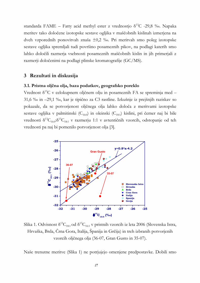
Vrednost δ13C v celokupnem oljčnem olju in posameznih FA se spreminja med –
31,6 ‰ in –29,1 ‰, kar je tipično za C3 rastline. Izkušnje iz prejšnjih raziskav so
pokazale, da se potvorjenost oljčnega olja lahko določa z meritvami izotopske
sestave ogljika v palmitinski (C16:0) in oleinski (C18:1) kislini, pri čemer naj bi bile
vrednosti δ13C16:0:δ13C18:1 v razmerju 1:1 v avtentičnih vzorcih, odstopanje od teh
vrednosti pa naj bi pomenilo potvorjenost olja [3].
-32 -31 -30 -29 -28 -27 -26 -25
-32
-31
-30
-29
-28
-27
-26
-25
36-07
35-07
Gran Gusto
Slovenska Istra
Hrvaska
Brda
Crna Gora
Italija
Spanija
Grcija
y=0.8*x-4.2
13C
18:1 (‰
)
13
C16:0
(‰)
Slika 1. Odvisnost δ13C18:1 od δ13C16:1 v pristnih vzorcih iz leta 2006 (Slovenska Istra,
Hrvaška, Brda, Črna Gora, Italija, Španija in Grčija) in treh izbranih potvorjenih
vzorcih oljčnega olja (36-07, Gran Gusto in 35-07).
Naše trenutne meritve (Slika 1) ne potrjujejo omenjene predpostavke. Dobili smo
17
dobro korelacijo med vrednostmi δ13C16:0 in δ13C18:1 (r2 = 0.94; p < 0.0001), vendar
so vrednosti δ13C18:1 v povprečju za 1,7 ‰ višje kot δ13C16:0. Razlogi za odstopanja
so lahko različni in jih je potrebno še nadalje raziskati. Eden od glavnih razlogov je
vpliv sprememb klimatskih pogojev, ki se letno spreminjajo in vplivajo na naravne
vsebnosti ogljikovih izotopov.
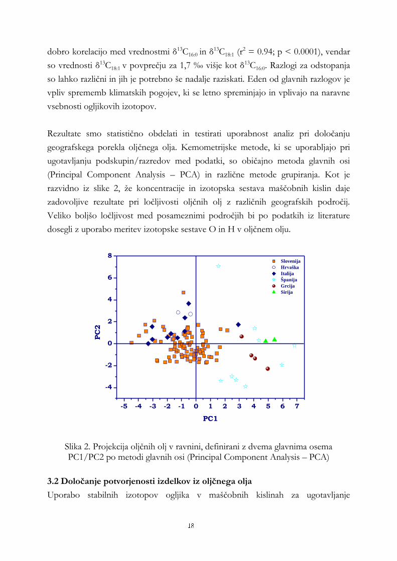
Rezultate smo statistično obdelati in testirati uporabnost analiz pri določanju
geografskega porekla oljčnega olja. Kemometrijske metode, ki se uporabljajo pri
ugotavljanju podskupin/razredov med podatki, so običajno metoda glavnih osi
(Principal Component Analysis – PCA) in različne metode grupiranja. Kot je
razvidno iz slike 2, že koncentracije in izotopska sestava maščobnih kislin daje
zadovoljive rezultate pri ločljivosti oljčnih olj z različnih geografskih področij.
Veliko boljšo ločljivost med posameznimi področjih bi po podatkih iz literature
dosegli z uporabo meritev izotopske sestave O in H v oljčnem olju.
-5 -4 -3 -2 -1 0 1 2 3 4 5 6 7
-4
-2
0
2
4
6
8 Slovenija
Hrvaška
Italija
Španija
Grcija
Sirija
PC
2
PC1
Slika 2. Projekcija oljčnih olj v ravnini, definirani z dvema glavnima osema PC1/PC2 po metodi glavnih osi (Principal Component Analysis – PCA)
3.2 Določanje potvorjenosti izdelkov iz oljčnega olja
Uporabo stabilnih izotopov ogljika v maščobnih kislinah za ugotavljanje
18
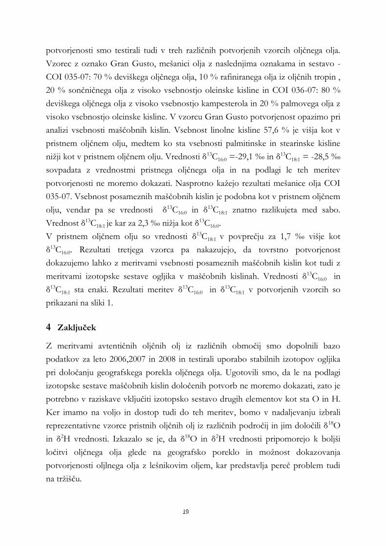
potvorjenosti smo testirali tudi v treh različnih potvorjenih vzorcih oljčnega olja.
Vzorec z oznako Gran Gusto, mešanici olja z naslednjima oznakama in sestavo -
COI 035-07: 70 % deviškega oljčnega olja, 10 % rafiniranega olja iz oljčnih tropin ,
20 % sončničnega olja z visoko vsebnostjo oleinske kisline in COI 036-07: 80 %
deviškega oljčnega olja z visoko vsebnostjo kampesterola in 20 % palmovega olja z
visoko vsebnostjo oleinske kisline. V vzorcu Gran Gusto potvorjenost opazimo pri
analizi vsebnosti maščobnih kislin. Vsebnost linolne kisline 57,6 % je višja kot v
pristnem oljčnem olju, medtem ko sta vsebnosti palmitinske in stearinske kisline
nižji kot v pristnem oljčnem olju. Vrednosti δ13C16:0 =-29,1 ‰ in δ13C18:1 = -28,5 ‰
sovpadata z vrednostmi pristnega oljčnega olja in na podlagi le teh meritev
potvorjenosti ne moremo dokazati. Nasprotno kažejo rezultati mešanice olja COI
035-07. Vsebnost posameznih maščobnih kislin je podobna kot v pristnem oljčnem
olju, vendar pa se vrednosti δ13C16:0 in δ13C18:1 znatno razlikujeta med sabo.
Vrednost δ13C18:1 je kar za 2,3 ‰ nižja kot δ13C16:0.
V pristnem oljčnem olju so vrednosti δ13C18:1 v povprečju za 1,7 ‰ višje kot
δ13C16:0. Rezultati tretjega vzorca pa nakazujejo, da tovrstno potvorjenost
dokazujemo lahko z meritvami vsebnosti posameznih maščobnih kislin kot tudi z
meritvami izotopske sestave ogljika v maščobnih kislinah. Vrednosti δ13C16:0 in
δ13C18:1 sta enaki. Rezultati meritev δ13C16:0 in δ13C18:1 v potvorjenih vzorcih so
prikazani na sliki 1.
4 Zaključek
Z meritvami avtentičnih oljčnih olj iz različnih območij smo dopolnili bazo
podatkov za leto 2006,2007 in 2008 in testirali uporabo stabilnih izotopov ogljika
pri določanju geografskega porekla oljčnega olja. Ugotovili smo, da le na podlagi
izotopske sestave maščobnih kislin določenih potvorb ne moremo dokazati, zato je
potrebno v raziskave vključiti izotopsko sestavo drugih elementov kot sta O in H.
Ker imamo na voljo in dostop tudi do teh meritev, bomo v nadaljevanju izbrali
reprezentativne vzorce pristnih oljčnih olj iz različnih področij in jim določili δ18O
in δ2H vrednosti. Izkazalo se je, da δ18O in δ2H vrednosti pripomorejo k boljši
ločitvi oljčnega olja glede na geografsko poreklo in možnost dokazovanja
potvorjenosti oljlnega olja z lešnikovim oljem, kar predstavlja pereč problem tudi
na tržišču.
19
Tovrstne raziskave podpirajo razvoj sistema za monitoring prehrambnih
proizvodov in razvoj metod za izvajanje kontrole živil. Z možnostjo dokazovanja
avtentičnosti oljčnega olja v prehrambnih izdelkih bodo pristojni organi zaščitili in
zavarovali kakovost oljčnih proizvodov hkrati pa tudi zaščitili potrošnika pred
morebitnimi potvorbami.
Literatura
[1] http://www.oljcno-olje.com/index.php?option=com_content&view=article&id=49&Itemid=64
[2] N. Ogrinc in sod.. Primerjava in razvoj novih metod za določanje avtentičnosti olja in prehrambenih izdelkov; zaključno poročilo o rezultatih opravljenega raziskovalnega dela elektronski vir, 2008.
[3] J. E. Spangenberg, N. Ogrinc. Authentication of vegetable oils by bulk and molecular carbon isotope analyses with emphasis on olive oil and pumpkin seed oil, J. Agric. Food Chem. 1534-1540 (49), 2001.
[4] N. Ogrinc, M. Gams Petrišič, M. Bučar-Miklavčič. Uporaba stabilnih izotopov ogljika pri določanju geografskega porekla in pristnosti oljčnega olja. Knjiga povzetkov /15. mednarodni simpozij Spektroskopija v teoriji in praksi, Nova Gorica, Slovenija, 18.-21. april 2007
20

Za širši interes
Potreba po spremljanju avtentičnosti in kakovosti prehrambnih izdelkov je
povzročila, da se je pojavilo povpraševanje po metodah, s katerimi bi dokazali
potvorjenost. Za odkrivanje ponarejanja živil se torej lahko poslužujemo tako
imenovanega globalnega pristopa, pri katerem določamo oporečnost na osnovi
fizikalno-kemijskih lastnostih vzorca. Te metode temeljijo na tako imenovanem
izotopskem prstnem odtisu ali »fingerprintingu«. Z njimi ne določamo le stopnjo in
način potvorjenosti, temveč tudi geografsko poreklo in celo leto proizvodnje
izdelka. Poleg oljčnega olja smo v raziskave avtentičnosti prehrambnih izdelkov
vključili tudi vina, med, sladkor, sadne sokove, ustekleničene vode in mleko ter
mlečne izdelke. Omenjene analize prispevajo h kakovosti oziroma certificiranju
določenih prehrambnih izdelkov in s tem k okrepitvi konkurenčne sposobnosti
agro-živilske industrije.
21
Results of coal gas desorption experiments, laboratory sorption experiments on lignite samples and in-situ seam gas pressure - rock stress measurements
Sergej Jamnikar1, Jerneja Lazar1, Simon Zavšek1, Ludvik Golob1
1 Coal Mine Velenje, Partizanska 78, Velenje, Slovenia
Abstract. Understanding the principles of coal seam gas behaviour require a
great number of experimental tests, monitoring campaigns, equipment design
and numerous correlations between gained data. Research work on Velenje
lignite and “in-situ” monitoring on long-wall faces consisted of coal’s gas
content experiments and mine monitoring campaigns. Gas content is
commonly measured with standard desorption methods by using direct
method which measures actual released gas volume from sample. According to
some widely-known methods (US Bureau of Mines direct method, Australian
Standard method), gas content determination methodology for Velenje lignite
was developed. Mine monitoring included seam gas pressure and rock stress
measurements, accompanied by gas sampling for composition and isotopic
analysis. Observations showed definite correlations between listed parameters
when measured results were combined into combined analysis.
Keywords: Coal seam gas, desorption experiments, seam gas pressure,
rock stress.
1 Introduction
Coal mining in thick lignite seams by using long-wall mining methodologies is an
approach towards efficient and effective way of coal deposits extraction. By
expanding the size of long-wall face, the amount of crushed coal often cause
increased additional releases of coal seam gases (carbon dioxide, methane) and
possible rock bursts, often accompanied by gas outbursts [1]. Lignite seam at Coal
Mine Velenje represents large volume reservoir for coal seam gases. Carbon dioxide
represents major share in total gas balance and is mostly adsorbed to coal or is
trapped in micro-pores of the coal structure, while methane is accumulated by the
22
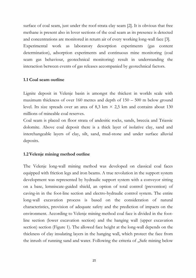
surface of coal seam, just under the roof-strata clay seam [2]. It is obvious that free
methane is present also in lover sections of the coal seam as its presence is detected
and concentrations are monitored in return air of every working long-wall face [3].
Experimental work as laboratory desorption experiments (gas content
determination), adsorption experiments and continuous mine monitoring (coal
seam gas behaviour, geotechnical monitoring) result in understanding the
interaction between events of gas releases accompanied by geotechnical factors.
1.1 Coal seam outline
Lignite deposit in Velenje basin is amongst the thickest in worlds scale with
maximum thickness of over 160 metres and depth of 150 – 500 m below ground
level. Its size spreads over an area of 8,3 km × 2,5 km and contains about 130
millions of mineable coal reserves.
Coal seam is placed on floor strata of andesitic rocks, sands, breccia and Triassic
dolomite. Above coal deposit there is a thick layer of isolative clay, sand and
interchangeable layers of clay, silt, sand, mud-stone and under surface alluvial
deposits.
1.2 Velenje mining method outline
The Velenje long-wall mining method was developed on classical coal faces
equipped with friction legs and iron beams. A true revolution in the support system
development was represented by hydraulic support system with a conveyor sitting
on a base, lemniscate-guided shield, an option of total control (prevention) of
caving-in in the foot-line section and electro-hydraulic control system. The entire
long-wall excavation process is based on the consideration of natural
characteristics, provision of adequate safety and the prediction of impacts on the
environment. According to Velenje mining method coal face is divided in the foot-
line section (lower excavation section) and the hanging wall (upper excavation
section) section (Figure 1). The allowed face height at the long-wall depends on the
thickness of clay insulating layers in the hanging wall, which protect the face from
the inrush of running sand and water. Following the criteria of „Safe mining below
23
water bearing strata at Velenje Coal Mine” the allowed working height is calculated
according to preliminary stated variations.
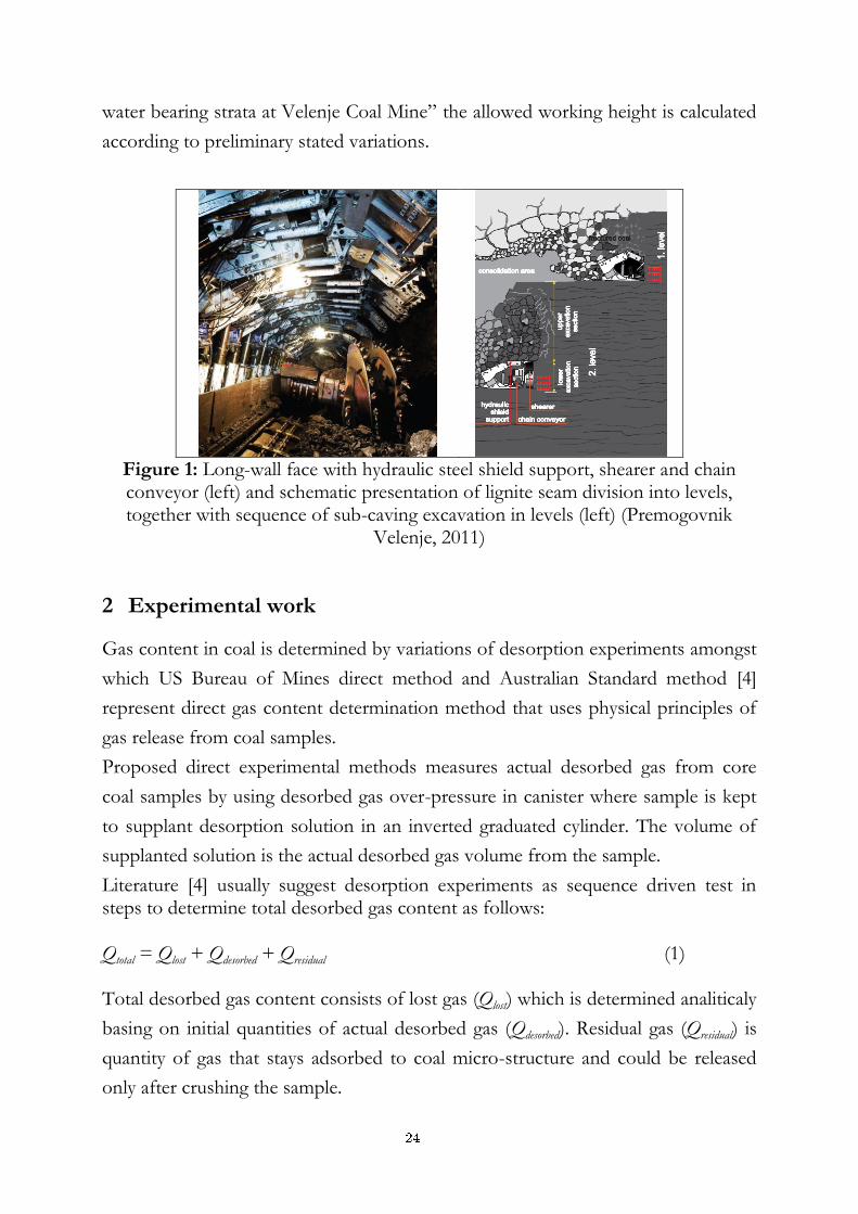
Figure 1: Long-wall face with hydraulic steel shield support, shearer and chain conveyor (left) and schematic presentation of lignite seam division into levels, together with sequence of sub-caving excavation in levels (left) (Premogovnik
Velenje, 2011)
2 Experimental work
Gas content in coal is determined by variations of desorption experiments amongst
which US Bureau of Mines direct method and Australian Standard method [4]
represent direct gas content determination method that uses physical principles of
gas release from coal samples.
Proposed direct experimental methods measures actual desorbed gas from core
coal samples by using desorbed gas over-pressure in canister where sample is kept
to supplant desorption solution in an inverted graduated cylinder. The volume of
supplanted solution is the actual desorbed gas volume from the sample.
Literature [4] usually suggest desorption experiments as sequence driven test in steps to determine total desorbed gas content as follows: Qtotal = Qlost + Qdesorbed + Qresidual (1) Total desorbed gas content consists of lost gas (Qlost) which is determined analiticaly
basing on initial quantities of actual desorbed gas (Qdesorbed). Residual gas (Qresidual) is
quantity of gas that stays adsorbed to coal micro-structure and could be released
only after crushing the sample.
24
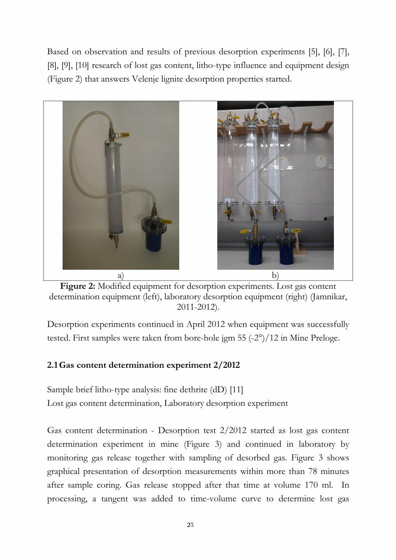
Based on observation and results of previous desorption experiments [5], [6], [7],
[8], [9], [10] research of lost gas content, litho-type influence and equipment design
(Figure 2) that answers Velenje lignite desorption properties started.
a) b)
Figure 2: Modified equipment for desorption experiments. Lost gas content determination equipment (left), laboratory desorption equipment (right) (Jamnikar,
2011-2012).
Desorption experiments continued in April 2012 when equipment was successfully
tested. First samples were taken from bore-hole jgm 55 (-2°)/12 in Mine Preloge.
2.1 Gas content determination experiment 2/2012
Sample brief litho-type analysis: fine dethrite (dD) [11]
Lost gas content determination, Laboratory desorption experiment
Gas content determination - Desorption test 2/2012 started as lost gas content
determination experiment in mine (Figure 3) and continued in laboratory by
monitoring gas release together with sampling of desorbed gas. Figure 3 shows
graphical presentation of desorption measurements within more than 78 minutes
after sample coring. Gas release stopped after that time at volume 170 ml. In
processing, a tangent was added to time-volume curve to determine lost gas
25
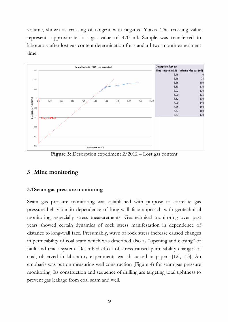
volume, shown as crossing of tangent with negative Y-axis. The crossing value
represents approximate lost gas value of 470 ml. Sample was transferred to
laboratory after lost gas content determination for standard two-month experiment
time.
Desorption_lost gas
Time_test (min0,5) Volume_des gas (ml)
5,48 0
5,48 75
5,66 100
5,83 110
5,92 120
6,00 125
6,32 130
7,00 140
7,55 150
7,87 160
8,83 170
Figure 3: Desorption experiment 2/2012 – Lost gas content
3 Mine monitoring
3.1 Seam gas pressure monitoring Seam gas pressure monitoring was established with purpose to correlate gas
pressure behaviour in dependence of long-wall face approach with geotechnical
monitoring, especially stress measurements. Geotechnical monitoring over past
years showed certain dynamics of rock stress manifestation in dependence of
distance to long-wall face. Presumably, wave of rock stress increase caused changes
in permeability of coal seam which was described also as “opening and closing” of
fault and crack system. Described effect of stress caused permeability changes of
coal, observed in laboratory experiments was discussed in papers [12], [13]. An
emphasis was put on measuring well construction (Figure 4) for seam gas pressure
monitoring. Its construction and sequence of drilling are targeting total tightness to
prevent gas leakage from coal seam and well.
26
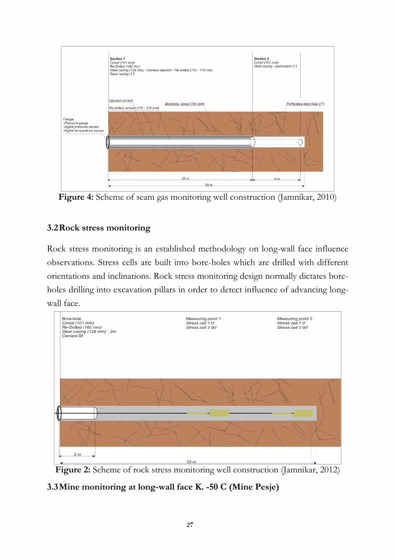
Figure 4: Scheme of seam gas monitoring well construction (Jamnikar, 2010)
3.2 Rock stress monitoring Rock stress monitoring is an established methodology on long-wall face influence
observations. Stress cells are built into bore-holes which are drilled with different
orientations and inclinations. Rock stress monitoring design normally dictates bore-
holes drilling into excavation pillars in order to detect influence of advancing long-
wall face.
Figure 2: Scheme of rock stress monitoring well construction (Jamnikar, 2012)
3.3 Mine monitoring at long-wall face K. -50 C (Mine Pesje)
27
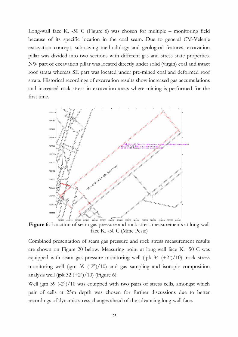
Long-wall face K. -50 C (Figure 6) was chosen for multiple – monitoring field
because of its specific location in the coal seam. Due to general CM-Velenje
excavation concept, sub-caving methodology and geological features, excavation
pillar was divided into two sections with different gas and stress state properties.
NW part of excavation pillar was located directly under solid (virgin) coal and intact
roof strata whereas SE part was located under pre-mined coal and deformed roof
strata. Historical recordings of excavation results show increased gas accumulations
and increased rock stress in excavation areas where mining is performed for the
first time.
Figure 6: Location of seam gas pressure and rock stress measurements at long-wall
face K. -50 C (Mine Pesje)
Combined presentation of seam gas pressure and rock stress measurement results
are shown on Figure 20 below. Measuring point at long-wall face K. -50 C was
equipped with seam gas pressure monitoring well (jpk 34 (+2˚)/10), rock stress
monitoring well (jgm 39 (-2)/10) and gas sampling and isotopic composition
analysis well (jpk 32 (+2˚)/10) (Figure 6).
Well jgm 39 (-2)/10 was equipped with two pairs of stress cells, amongst which
pair of cells at 25m depth was chosen for further discussions due to better
recordings of dynamic stress changes ahead of the advancing long-wall face.
28
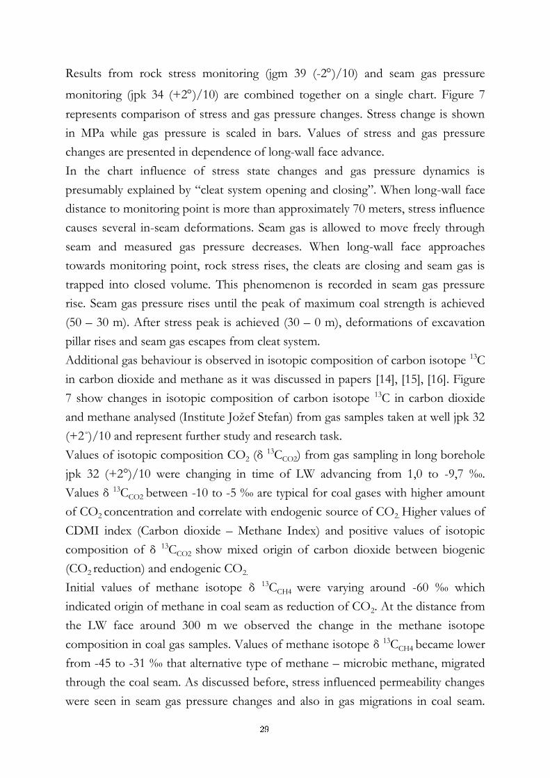
Results from rock stress monitoring (jgm 39 (-2)/10) and seam gas pressure
monitoring (jpk 34 (+2)/10) are combined together on a single chart. Figure 7
represents comparison of stress and gas pressure changes. Stress change is shown
in MPa while gas pressure is scaled in bars. Values of stress and gas pressure
changes are presented in dependence of long-wall face advance.
In the chart influence of stress state changes and gas pressure dynamics is
presumably explained by “cleat system opening and closing”. When long-wall face
distance to monitoring point is more than approximately 70 meters, stress influence
causes several in-seam deformations. Seam gas is allowed to move freely through
seam and measured gas pressure decreases. When long-wall face approaches
towards monitoring point, rock stress rises, the cleats are closing and seam gas is
trapped into closed volume. This phenomenon is recorded in seam gas pressure
rise. Seam gas pressure rises until the peak of maximum coal strength is achieved
(50 – 30 m). After stress peak is achieved (30 – 0 m), deformations of excavation
pillar rises and seam gas escapes from cleat system.
Additional gas behaviour is observed in isotopic composition of carbon isotope 13C
in carbon dioxide and methane as it was discussed in papers [14], [15], [16]. Figure
7 show changes in isotopic composition of carbon isotope 13C in carbon dioxide
and methane analysed (Institute Jožef Stefan) from gas samples taken at well jpk 32
(+2˚)/10 and represent further study and research task.
Values of isotopic composition CO2 (δ 13CCO2) from gas sampling in long borehole
jpk 32 (+2°)/10 were changing in time of LW advancing from 1,0 to -9,7 ‰.
Values δ 13CCO2 between -10 to -5 ‰ are typical for coal gases with higher amount
of CO2 concentration and correlate with endogenic source of CO2. Higher values of
CDMI index (Carbon dioxide – Methane Index) and positive values of isotopic
composition of δ 13CCO2 show mixed origin of carbon dioxide between biogenic
(CO2 reduction) and endogenic CO2.
Initial values of methane isotope δ 13CCH4 were varying around -60 ‰ which
indicated origin of methane in coal seam as reduction of CO2. At the distance from
the LW face around 300 m we observed the change in the methane isotope
composition in coal gas samples. Values of methane isotope δ 13CCH4 became lower
from -45 to -31 ‰ that alternative type of methane – microbic methane, migrated
through the coal seam. As discussed before, stress influenced permeability changes
were seen in seam gas pressure changes and also in gas migrations in coal seam.
29
Alternative values remained the same until methane escape through the rock stress
caused cleat/ porous system. After structure deformation, original gas state with
low values of isotopes δ 13CCH4 was observed [3].
Figure 7: Relation between seam gas pressure and rock stress state change in
dependence of distance to long-wall face. Rapid increase of stress at distances 305 m and 125 m represent stress cell settings with additional fluid injection.
4 Conclusions and future work
Investigation in field of desorption and gas content determination included review
of knowledge, experiments and methodology on field in world’s scale, experiments,
performed on samples from Coal Mine Velenje and methodology and equipment
design that match Velenje lignite properties.
Desorption experiments included repetitions of experiments from previous
campaigns, followed by modifications in sample treatment (crushing) and lost gas
content determinations.
Mine monitoring was divided into seam gas pressure measurements and rock stress
measurements for which dedicated measurement methodology and monitoring
objects were developed. Results of both were combined after data interpretations
30
showed possible correlations that were assumed even before seam gas pressure
monitoring was established.
In addition, seam gas pressure and rock stress measurements interpretations were
accompanied with seam gas and isotopic composition results that describe
migration principles of coal seam gases.
References:
[1] J. Likar. Analiza mehanizmov nenadnih izbruhov premoga in plina v premogovnikih, 1995. Univerza v Ljubljani, Fakulteta za naravoslovje in tehnologijo, Oddelek za montanistiko. Ph.D. Dissertation.
[2] T. Kanduč. Izotopske značilnosti premogovega plina v velenjskem bazenu, (2004). University of Ljubljana, Faculty of natural sciences and engineering department of geology. M. Sc. Dissertation.
[3] S. Jamnikar, J. Lazar, R. Lah, J. Žula, E. Burič, S. Zavšek. Poročila o spremljanju tehnoloških, plinskih in geotehničnih parametrov na odkopih G2/B, K. -50 A, K. -120 B, K. -50 B, G 2/C, K.-50 C. 2008 – 2012. Premogovnik Velenje. Report.
[4] W.P. Diamond, S. Schatzel. Measuring the gas content of coal: A review., 1986. International Journal of Coal Geology 35 (1998), 311-331. Paper.
[5] J. Likar, M. Ulrich-Obal. Poročilo o kontrolnem testiranju desorbimetrov z mešali, 1997. IRGO, Ljubljana. Report.
[6] J. Likar, M. Ulrich, M. Zahornik. Laboratorijski desorbimeter, 1997. IRGO, Ljubljana. Report.
[7] J. Pezdič, M. Markič, M. Letič, A. Popovič, S. Zavšek. Laboratory simulation of desorption – desorption processes on different lignite lithotypes from Velenje lignite mine, 1999, RMZ – Materials and Geoenviroment, Vol. 46, No. 3, 555-568, Paper.
[8] A. Zapušek, D. Dimec, M. Videmšek, E. Burič, J. Jezeršek. Vrtina 933 T/96: Rezultati meritev desorbiranih plinov, 1997. ERICo, Velenje. Report.
[9] A. Zapušek, V. Landekar, E. Burič. Vrtini 759 T/98 in 770-K/98: Rezultati meritev desorbiranih plinov, 1999. ERICo, Velenje. Report.
[10] S. Jamnikar. Desorption properties of Velenje lignite and measurement methodology development, 2011. 4th Balkan Mining Congress, Paper’s book, 165 – 172. Paper.
[11] M. Markič. Petrology and genesis of the Velenje lignite, (2009). University of Ljubljana, Faculty of natural sciences and engineering department of geology. Ph.D. Dissertation.
[12] S. Durucan, and J.S. Edwards. The Effects of Stress and Fracturing on Permeability of Coal, 1986. Mining Science and Technology, 3, 205-216. Paper.
[13] R. Konečny, jr., A. Kožušnikova, P. Martinec. Rock mass as a porous medium: Gas filtration ability in triaxial state of stress. Institute of Geonics ASCR, Ostrava, Czech Republic. Proceedings of the International Congress on Rock Mechanics, Paris, 1999. Paper.
[14] T. Kanduč. Izotopske značilnosti premogovega plina v velenjskem bazenu, (2004). University of Ljubljana, Faculty of natural sciences and engineering department of geology. M. Sc. Dissertation.
[15] T. Kanduč, J. Pezdič. Origin and distribution of coalbed gases from the Velenje basin, Slovenia, 2005. Geochemical Journal, Vol.39.
[16] T. Kanduč, J. Pezdič, S. Lojen, S. Zavšek. Study of the gas composition ahead of the working face in a lignite seam from the Velenje basin. RMZ – Materials and Geoenviroment. Paper.
31

For wider interest
Underground coal mining still represents hazardous operations and dealing with
natural forces amongst which coal and rock-bursts represent possible threats for
miner’s safety.
Research into hazardous events prevention precautions consists from coal gas
content determination experiments and mine monitoring campaigns of gas
behaviour analysis and coal excavation influence on surrounding coal masses.
Mine monitoring included seam gas pressure and rock stress measurements,
accompanied by gas sampling for composition and isotopic analysis. Observations
showed definite correlations between listed parameters when measured results were
combined into combined analysis.
Research work is targeting final result - understanding coal seam properties
concerning gas behaviour and rock stress distribution influence that answers
challenge of underground gas drainage of coal seam.
32
Jedkanje PET filmov v poznem porazelektritvenem delu kisikove plazme
Metod Kolar1,2,3, Darij Kreuh1, Alenka Vesel2,3, Miran Mozetič2,3, Karin
Stana - Kleinschek4
1 Ekliptik d.o.o., Teslova ulica 30, 1000 Ljubljana
2 Odsek za tehnologijo površin in optoelektroniko, Institut "Jožef Stefan", Jamova
39, 1000 Ljubljana,
3 Mednarodna podiplomska šola Jožefa Stefana, Jamova 39, 1000 Ljubljana
4 Fakulteta za strojništvo, Univerza v Mariboru, Smetanova ul. 17, 2000 Maribor
Povzetek. Praktična uporaba polimernih materialov v medicini je še vedno
omejena s specifičnimi lastnostmi teh materialov. Pri uporabi polietilen
tereftalata (PET) za umetne žile in katetre se soočamo s problemom vezave
bioloških substanc na površino polimernih materialov. Po naši hipotezi lahko
ta problem bistveno zmanjšamo z uporabo reaktivnih plazemskih delcev.
Delci reagirajo s površino polimera tako, da odstranijo sledove organskih
nečistoč, obenem pa zmanjšajo vezavo proteinov. Za razvoj ustreznega
industrijskega postopka pa ključno težavo predstavlja jedkanje materiala. Da bi
natančno določili vpliv nevtralnih kisikovih atomov na jedkanje PET-a smo
opravili raziskave, ki so opisane v tem prispevku. Z zelo natančno metodo
kremenove mikrotehtnice z enoto merjenja dušenja nihanja (QCM-D)
smo izmerili hitrost jedkanja PET materiala v porazelektritvenem delu kisikove
plazme in ugotovili, da je le ta odvisna od vzbujevalne moči in postane pri
večjih močeh konstantna z vrednostjo okoli 1 nm/min. Rezultati kažejo, da je
tovrstna obdelava uporabna v medicinski praksi, saj je hitrost jedkanja
bistveno manjša za polimer kot za organske nečistoče.
Ključne besede: jedkanje, organski materiali, plazma, PET.
1 Uvod
Plazma je stanje plina, v katerem je znatni del molekul disociiran in ioniziran.
Prehod plina v stanje plazme lahko dosežemo na dva načina in sicer tako, da plin
33
segrejemo do tako visoke temperature, da znatni del atomov razpade na pozitivne
ione in elektrone, ali pa tako, da plin namestimo v močno električno polje, kjer se
prosti elektroni, ki so v vsakem primeru v plinu v majhnih gostotah, pospešijo in
ob neprožnih trkih z atomi ali molekulami le-te ionizirajo.
Obdelava materialov z nizko-temperaturno plazmo velja za eno najbolj
vsestranskih tehnik za pridobivanje edinstvenih lastnosti površin materialov, še
posebej polimernih. Zadnje čase poteka vse več raziskav obdelave organskih
materialov z neravnovesnimi nizko-temperaturnimi plinskimi plazmami, predvsem
zaradi možne uporabe v biomedicini. Znano je, da se pri obdelavi s kisikovo
plazmo na površini ustvarijo polarne funkcionalne skupine, površina materiala se
jedka, posledično se zato poveča hrapavost površine [1-5]. Čeprav je jedkanje s
plazmo znano že desetletja, natančen mehanizem tega pojava še ni znan. Bistven
razlog je v dejstvu, da v plazmi vselej nastajajo različne vrste reaktivnih delcev, kot
so molekularni in atomarni ioni, nevtralni atomi v osnovnem in vzbujenih stanjih,
ter nevtralne molekule v metastabilnih vzbujenih stanjih. Plazemska obdelava
polimerov je pogosto preveč agresivna, saj je zelo težko zagotoviti obdelavo pri
sobni temperaturi. Da bi rešili ta tehnološki problem, smo postavili hipotezo, po
kateri za dosego primernih učinkov kisikove plazme sploh ne potrebujemo, ampak
potrebujemo zgolj eno vrsto reaktivnih delcev, to so nevtralni kisikovi atomi v
osnovnem stanju. Predhodne raziskave v naši raziskovalni skupini so pokazale, da
lahko zagotovimo obdelavo materialov z nevtralnimi atomi tako, da obdelovanec
namestimo v pozni porazelektritveni del kisikove plazme [6, 7]. V
porazelektritvenem delu namreč električno nabiti delci in visoko vzbujeni atomi
niso prisotni, saj se na poti od plazme do porazelektritvenega dela nevtralizirajo oz.
deekscitirajo. Po naši hipotezi je interakcija atomov s površino obdelovanca dovolj
intenzivna, da odstranimo organske nečistoče in funkcionaliziramo površino
polimera, obenem pa dovolj šibka, da prepreči intenzivno jedkanje.
2 Metode in materiali
2.1 Priprava vzorcev
Modelne filme PET smo nanašali na kremenove substrate s tehniko vrtenja (spin-
coating). Folijo amorfnega polietilen tereftalata (Goodfellow, Cambridge, Velika
34
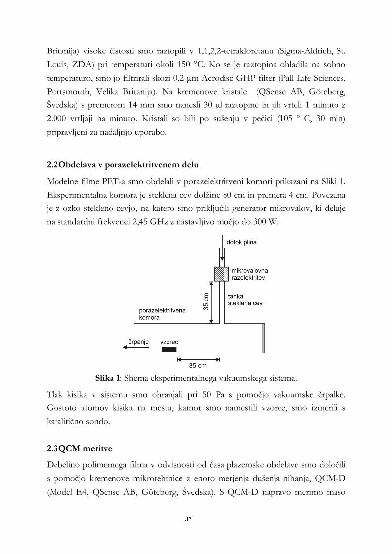
Britanija) visoke čistosti smo raztopili v 1,1,2,2-tetrakloretanu (Sigma-Aldrich, St.
Louis, ZDA) pri temperaturi okoli 150 °C. Ko se je raztopina ohladila na sobno
temperaturo, smo jo filtrirali skozi 0,2 μm Acrodisc GHP filter (Pall Life Sciences,
Portsmouth, Velika Britanija). Na kremenove kristale (QSense AB, Göteborg,
Švedska) s premerom 14 mm smo nanesli 30 µl raztopine in jih vrteli 1 minuto z
2.000 vrtljaji na minuto. Kristali so bili po sušenju v pečici (105 º C, 30 min)
pripravljeni za nadaljnjo uporabo.
2.2 Obdelava v porazelektritvenem delu
Modelne filme PET-a smo obdelali v porazelektritveni komori prikazani na Sliki 1.
Eksperimentalna komora je steklena cev dolžine 80 cm in premera 4 cm. Povezana
je z ozko stekleno cevjo, na katero smo priključili generator mikrovalov, ki deluje
na standardni frekvenci 2,45 GHz z nastavljivo močjo do 300 W.
Slika 1: Shema eksperimentalnega vakuumskega sistema.
Tlak kisika v sistemu smo ohranjali pri 50 Pa s pomočjo vakuumske črpalke.
Gostoto atomov kisika na mestu, kamor smo namestili vzorce, smo izmerili s
katalitično sondo.
2.3 QCM meritve
Debelino polimernega filma v odvisnosti od časa plazemske obdelave smo določili
s pomočjo kremenove mikrotehtnice z enoto merjenja dušenja nihanja, QCM-D
(Model E4, QSense AB, Göteborg, Švedska). S QCM-D napravo merimo maso
35
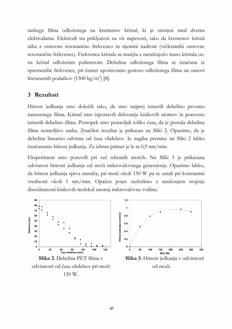
tankega filma odloženega na kremenov kristal, ki je stisnjen med dvema
elektrodama. Elektrodi sta priključeni na vir napetosti, tako da kremenov kristal
niha z osnovno resonančno frekvenco in njenimi nadtoni (večkratniki osnovne
resonančne frekvence). Frekvenca kristala se manjša z naraščajočo maso kristala oz.
na kristal odloženim polimerom. Debelina odloženega filma se izračuna iz
spremembe frekvence, pri čemer upoštevamo gostoto odloženega filma na osnovi
literaturnih podatkov (1300 kg/m3) [8].
3 Rezultati
Hitrost jedkanja smo določili tako, da smo najprej izmerili debelino prvotno
nanesenega filma. Kristal smo izpostavili delovanju kisikovih atomov in ponovno
izmerili debelino filma. Postopek smo ponavljali toliko časa, da je postala debelina
filma nemerljivo tanka. Značilen rezultat je prikazan na Sliki 2. Opazimo, da je
debelina linearno odvisna od časa obdelave. Iz nagiba premice na Sliki 2 lahko
izračunamo hitrost jedkanja. Za izbran primer je le ta 0,9 nm/min.
Eksperiment smo ponovili pri več izbranih močeh. Na Sliki 3 je prikazana
odvisnost hitrosti jedkanja od moči mikrovalovnega generatorja. Opazimo lahko,
da hitrost jedkanja sprva narašča, pri moči okoli 150 W pa se ustali pri konstantni
vrednosti okoli 1 nm/min. Opažen pojav razložimo z nasičenjem stopnje
disociiranosti kisikovih molekul znotraj mikrovalovne votline.
Slika 2: Debelina PET filma v
odvisnosti od časa obdelave pri moči
150 W.
Slika 3: Hitrost jedkanja v odvisnosti
od moči.
36
4 Zaključek
Rezultati naših meritev kažejo, da je izbrani polimerni material dobro odporen na
jedkanje z nevtralnimi kisikovimi atomi. Za razliko od obdelave v plazmi, kjer smo
opazili izredno agresivno jedkanje [9-11], je hitrost jedkanja v porazelektritvenem
delu za dva velikostna reda manjša. Ker je hitrost jedkanja organskih nečistoč [12],
ki se značilno nahajajo na površini katetrov, bistveno večja, lahko sklepamo, da je
metoda obdelave v porazelektritvenem delu primerna za čiščenje katetrov po
uporabi v medicinski praksi. Z atomi kisika lahko torej odstranimo nečistoče, ne da
bi bistveno spremenili prvotne lastnosti katetra.
Operacijo delno financira Evropska unija, in sicer iz Evropskega socialnega sklada.
Literatura:
[1] A. Vesel, K. Eleršič, I. Junkar, in B. Malič. Modification of a polyethylene naphthalate polymer using an oxygen plasma treatment. Mater. Tehnol., 43(6): 323-326, 2009.
[2] C. M. Chan, T. M. Ko, H. Hiraoka. Polymer surface modification by plasmas and photons. Surface Science Reports, 24(1-2): 1-54, 1996.
[3] A. Vesel, M. Mozetic, A. Hladnik, J. Dolenc, J. Zule, S. Milosevic, N. Krstulovic, M. Klanjšek-Gunde, N. Hauptmann. Modification of ink-jet paper by oxygen-plasma treatment. Journal of Physics D: Applied Physics, 40(12): 3689-3696, 2007.
[4] V. Hody, T. Belmonte, T. Czerwiec, G. Henrion, J. M. Thiebaut. Oxygen grafting and etching of hexatriacontane in late N2–O2 post-discharges. Thin Solid Films, 506-507: 212-216, 2006.
[5] T. Belmonte, C. D. Pintassilgo, T. Czerwiec, G. Henrion, V. Hody, J. M. Thiebaut, J. Loureiro. Oxygen plasma surface interaction in treatments of polyolefines. Surf. Coat. Technol., 200(1-4): 26-30, 2005.
[6] G. Primc, R. Zaplotnik, A. Vesel, M. Mozetic. Microwave discharge as a remote source of neutral oxygen atoms. AIP Advances, 1(2): 022129, 2011.
[7] M. Mozetič. Surface modification of materials using an extremely non-equilibrium oxygen plasma. Mater. Tehnol., 44(4): 165-171, 2010.
[8] Polyethylene terephthalate - online catalogue source - supplier of research materials in small quantities - Goodfellow, http://www.goodfellow.com/E/Polyethylene-terephthalate.html, 2012.
[9] A. Doliška, A. Vesel, M. Kolar, K. Stana-Kleinschek, M. Mozetič. Interaction between model poly(ethylene terephthalate) thin films and weakly ionised oxygen plasma. Surf. Int. Anal., 44(1): 56-61, 2012.
[10] I. Junkar, A. Vesel, U. Cvelbar, M. Mozetic, S. Strnad. Influence of oxygen and nitrogen plasma treatment on polyethylene terephthalate (PET) polymers. Vacuum, 84(1): 83-85, 2009.
[11] I. Junkar, U. Cvelbar, A. Vesel, N. Hauptman, M. Mozetič. The Role of Crystallinity on Polymer Interaction with Oxygen Plasma. Plasma Processes Polym., 6(10): 667-675, 2009.
[12] U. Cvelbar, M. Mozetič, N. Hauptman, M. Klanjšek-Gunde. Degradation of Staphylococcus aureus bacteria by neutral oxygen atoms. J. Appl. Phys., 106(10): 103303, 2009.
37
Za širši interes
Na odseku za tehnologijo površin in optoelektroniko Instituta "Jožef Stefan"
raziskovalci razvijajo metode za modifikacijo površin različnih materialov s
termodinamsko zelo neravnovesno plinsko plazmo. Industrijski partnerji
potrebujejo tovrstne tehnologije za izboljšanje kakovosti svojih izdelkov in
nadomeščanje okolju neprijaznih tehnoloških postopkov. Za različne partnerje so
razvili tehnološke postopke plazemskega čiščenja, selektivnega plazemskega
jedkanja, površinske funkcionalizacije in hladnega upepeljevanja. V zadnjem času se
predvsem ukvarjajo z modifikacijo površinskih lastnosti polimernih materialov, ki
se uporabljajo v medicini. Originalne tehnološke postopke zaščitijo z
mednarodnimi patenti, znanstvena odkritja pa objavljajo v vrhunskih specializiranih
revijah.
Moja vloga v raziskovalni skupini, ki je izrazito interdisciplinarna, je razvoj
postopkov za modifikacijo površine umetnih žil, s ciljem izboljšanja
biokompatibilnosti. Umetne žile, ki se trenutno uporabljajo, imajo sicer odlične
kemijske in mehanske lastnosti, žal pa prepogosto povzročajo različne po-
operativne zaplete, kamor v prvi vrsti sodi tromboza. Preliminarne raziskave so
pokazale, da je mogoče s primerno funkcionalizacijo notranje površine umetnih žil
bistveno zmanjšati aktivacijo trombocitov in s tem nastajanje krvnih strdkov. Da bi
inovativni tehnološki postopek uporabili v medicinski praksi, je potrebno opraviti
obsežne temeljne raziskave, ki bi omogočile vpogled v izredno zahteven pojav
kopičenja krvnih proteinov. V okviru svojega doktorskega izobraževanja je moja
naloga natančno določiti vpliv različnih reaktivnih kisikovih delcev na
funkcionalizacijo polimernih materialov za umetne žile, določiti intenzivnost
interakcije izbranih reaktivnih delcev s krvnimi proteini in določiti morebitne
poškodbe umetnih žil, ki so posledica interakcije obdelovancev z reaktivnimi delci.
Končni cilj mojih raziskav je optimizacija površinske modifikacije umetnih žil, ki bi
omogočila minimalno depozicijo krvnih proteinov ob hkratni izboljšani
biokompatibilnosti za pravilno vezavo endotelija na umetne žile.
38
Entirely renewable and self-sufficient municipal energy system
Anja Kostevšek1,2, Leon Cizelj3, Janez Petek4, Boris Sučić5, Matevž
Pušnik5, Aleksandra Pivec1
1 Scientific Research Centre Bistra Ptuj, Ptuj, Slovenia
2 Jožef Stefan International Postgraduate School, Ljubljana, Slovenia
3 Reactor Engineering Division, Jožef Stefan Institute, Ljubljana, Slovenia
4 Local Energy Agency Spodnje Podravje, Ptuj, Slovenia
5 Energy Efficiency Centre, Jožef Stefan Institute, Ljubljana, Slovenia
Abstract. Municipal energy system is recognized as the one of the major
development engines in greening the energy system. Integration of renewable
resources into the energy system is the most appropriate choice in an attempt
to decrease negative impacts on the environment. Various energy policies
define targets with inclusion of different shares of renewable resources in
specific time horizons. However, energy systems on 100% renewable supply
still represent a challenge. The main objective of this paper is to demonstrate
feasibility of the proposed renewable and self-sufficient municipal energy
system. Energy model is used for setting the reference energy system and
calculation of the scenarios. Performance of biomass, solar and renewable mix
scenarios were conducted for this research. The paper discusses only technical
aspects of the 100% renewable energy system.
Keywords: municipal energy system, renewable energy sources, renewable and
self-sufficient energy systems
1 Introduction
Decarbonisation of energy systems represents a major issue in today’s society. A
variety of possible pathways is being proposed. With energy policies on European
level additional targets were proposed, such as a 20% share of energy from
renewable sources in the gross final energy consumption by 2020, and a 10% share
39
of renewable energy specifically in the transport sector [1]. On the other hand,
some proposals are drafted to reach an 80% share from renewable energy sources
(RES) by 2050. In the frame of the European Union energy climate package
Slovenia set ambitious target by 2020 to achieve 25% renewable energy in the gross
final energy consumption. According to the new National Renewable Energy
Action Plan Slovenia1 would play an active role in the development and promotion
of the new technologies and solutions, which would enable wider usage of the
renewable energy sources in industry, public, residential and transport sectors [2].
In order to accomplish future energy objectives on European and national level,
additional work on local level has to be performed. The draft of Slovenian Energy
Program2 encourages the use of 100% renewable energy systems in five
municipalities by 2020 and twenty municipalities by 2030. The importance of
creation of a 100% renewable municipal energy system (MES) has also been
recognized elsewhere [3]. This paper presents performance of energy scenarios to
provide suitable structure of a 100% renewable and self-sufficient MES. The main
focus is to demonstrate the technical eligibility of the 100% renewable MES.
2 Methodology
2.1 Model development
The following step presents the selection of adequate energy planning tool for
generating future scenarios of MES. Several modeling tools are available for local
energy planning. In the Slovenian case, the decision was made on various
assumptions and experiences from the constitution of previous energy models.
MESAP (Modular Energy-System Analysis and Planning Environment) toolbox
was brought up because it covers all the relevant tools for building an appropriate
model for municipalities. The Reference Energy Environmental Model for
Municipalities (REES-MOL), which was created for the city of Ljubljana, the
capital of Slovenia, was transformed and adapted to calculate scenarios for
renewable energy system of Podlehnik municipality. The REES-MOL is energy
1 National Renewable Energy Action Plan Slovenia – National renewable energy action plan 2010-2020 (NREAP)
Slovenia, Ljubljana, July 2010. 2 Slovenian Energy Program – Proposal of the National Energy Programme of the Republic of Slovenia for the
2010-2030 Period, draft, Ljubljana, June 2010.
40
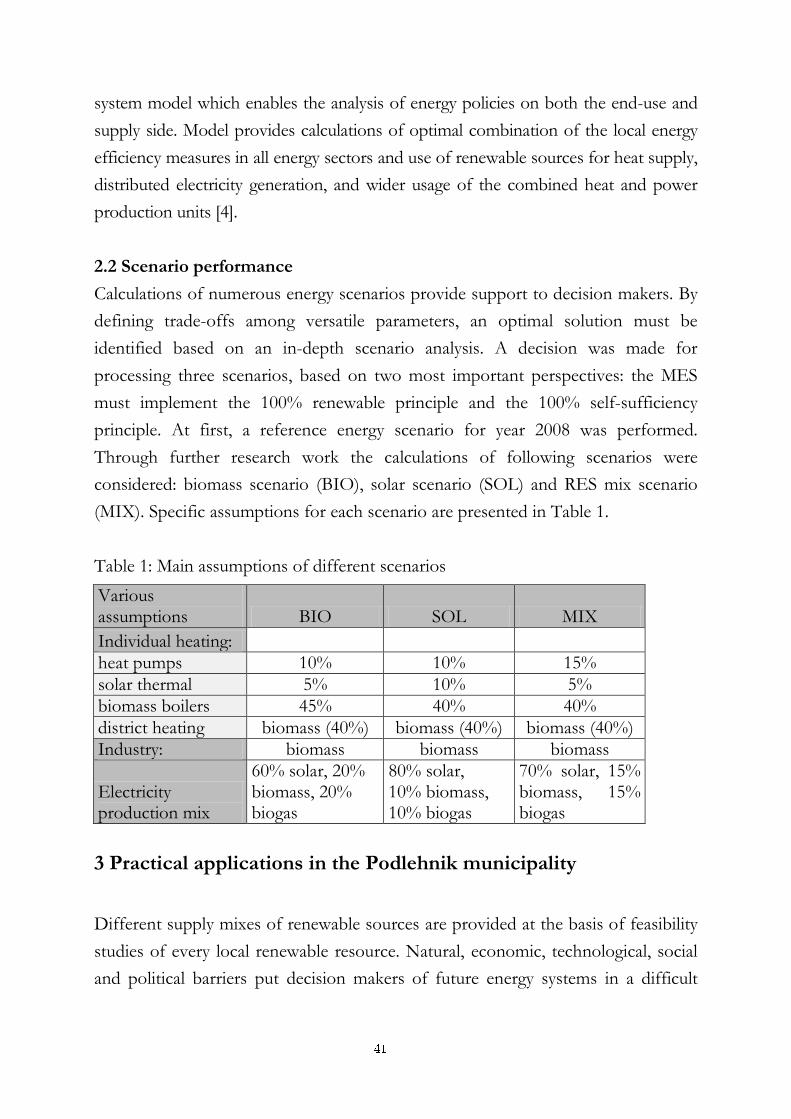
system model which enables the analysis of energy policies on both the end-use and
supply side. Model provides calculations of optimal combination of the local energy
efficiency measures in all energy sectors and use of renewable sources for heat supply,
distributed electricity generation, and wider usage of the combined heat and power
production units [4].
2.2 Scenario performance
Calculations of numerous energy scenarios provide support to decision makers. By
defining trade-offs among versatile parameters, an optimal solution must be
identified based on an in-depth scenario analysis. A decision was made for
processing three scenarios, based on two most important perspectives: the MES
must implement the 100% renewable principle and the 100% self-sufficiency
principle. At first, a reference energy scenario for year 2008 was performed.
Through further research work the calculations of following scenarios were
considered: biomass scenario (BIO), solar scenario (SOL) and RES mix scenario
(MIX). Specific assumptions for each scenario are presented in Table 1.
Table 1: Main assumptions of different scenarios
Various assumptions BIO SOL MIX
Individual heating:
heat pumps 10% 10% 15%
solar thermal 5% 10% 5%
biomass boilers 45% 40% 40%
district heating biomass (40%) biomass (40%) biomass (40%)
Industry: biomass biomass biomass
Electricity production mix
60% solar, 20% biomass, 20% biogas
80% solar, 10% biomass, 10% biogas
70% solar, 15% biomass, 15% biogas
3 Practical applications in the Podlehnik municipality
Different supply mixes of renewable sources are provided at the basis of feasibility
studies of every local renewable resource. Natural, economic, technological, social
and political barriers put decision makers of future energy systems in a difficult
41
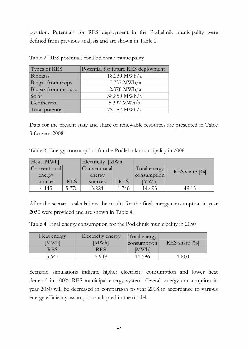
position. Potentials for RES deployment in the Podlehnik municipality were
defined from previous analysis and are shown in Table 2.
Table 2: RES potentials for Podlehnik municipality
Types of RES Potential for future RES deployment
Biomass 18.230 MWh/a
Biogas from crops 7.737 MWh/a
Biogas from manure 2.378 MWh/a
Solar 38.850 MWh/a
Geothermal 5.392 MWh/a
Total potential 72.587 MWh/a
Data for the present state and share of renewable resources are presented in Table
3 for year 2008.
Table 3: Energy consumption for the Podlehnik municipality in 2008
Heat [MWh] Electricity [MWh]
Total energy consumption
[MWh]
RES share [%] Conventional
energy sources RES
Conventional energy sources RES
4.145 5.378 3.224 1.746 14.493 49,15
After the scenario calculations the results for the final energy consumption in year
2050 were provided and are shown in Table 4.
Table 4: Final energy consumption for the Podlehnik municipality in 2050
Heat energy [MWh]
Electricity energy [MWh]
Total energy consumption
[MWh]
RES share [%]
RES RES
5.647 5.949 11.596 100,0
Scenario simulations indicate higher electricity consumption and lower heat
demand in 100% RES municipal energy system. Overall energy consumption in
year 2050 will be decreased in comparison to year 2008 in accordance to various
energy efficiency assumptions adopted in the model.
42
4 Discussion and conclusion
A modern MES with renewable supply mix differs in routes from present fossil
based energy systems. Integration of 100% renewable and self-sufficient principles
into MES presents the future goal of fighting climate change. The study confirmed
technical feasibility of constituting a 100% renewable and self-sufficient MES.
Assessment of scenarios should be performed on the basis of local conditions. On
behalf of presented scenarios, decision makers may be able to depict the proper
solution. For Podlehnik municipality the RES feasibility studies were included in
the Local Energy Concept. Only general predictions from various previous analyses
were presented. Further research would take place in defining more in-depth
studies for specific RES potentials. This research considers only technical aspects
of a 100% renewable MES. In the future perspective, also environmental, social
and economic aspects need to be included. Penetration of new technologies and
R&D activities in the field of renewable technologies will make an enormous
impact on the outlook of the 2050 MES. To conclude with, transfer towards a
100% renewable MES would require a sequential adaptation process in different
time horizons.
Acknowledgements
The research work of the corresponding author is supported by the European Slovenian
Technology Agency under tender Young researchers from industry. Operation is partly financed
by the European Union (European Social Fund).
References:
[1] The European Parliament and the Council of the European Union. Directive 2009/28/EC of
the European Parliament and of the council of 23 April 2009 on the promotion of the use of
energy from renewable sources, 2009.
[2] National Renewable Energy Action Plan 2010-2020.
http://ec.europa.eu/energy/renewables/transparency_platform/doc/national_renewable_energy
_action_plan_slovenia_en.pdf, 2010
[3] P. A. Østergaard, B. V. Mathiesen, B. Möller and H. Lund. A renewable energy scenario for
Aalborg Municipality based on low-temperature geothermal heat, wind power and biomass.
Energy, 35(12): 4892-4901, 2010
[4] Energy Efficiency Centre, Jozef Stefan Institute. Sustainable urban infrastructure-Ljubljana-
Prospectives by 2050. IJS, 2011.
43

For wider interest
Climate change mitigation activities support usage of renewable resources due to
their neutral impact on the environment. Various legislative acts stress the
important role of municipalities in accomplishing the energy targets. This is why
focus on municipality energy system and its development present a promising
future orientation. Forming energy system on entirely renewable resources presents
the new pathway, where the whole energy supply could be based on local supply
facilities. In practice, the results could be applied for other municipalities, smaller
local community, a district or a group of buildings. In addition, for concretizing the
system more technical studies should be revealed.
The case study was presented for Podlehnik municipal energy system. Analyses of
three different scenarios leading to entirely renewable energy system with mixes of
biomass, solar and electricity confirmed on the sufficiency of renewable resources.
The results confirmed the technical feasibility to develop an independent renewable
municipal energy system. Demonstration of possibilities to develop energy systems
on a 100% renewable and 100% local supply represents added value. In the future
several research activities should be focused in providing detailed analysis of
integration of renewable resources into energy supply chain from technical,
environmental, economic and social aspect.
44
Selenium and its distribution in edible mussel Mytilus galloprovincialis collected from different locations
Urška Kristan1,2, Vekoslava Stibilj1
1 Department of Environmental Sciences, Jožef Stefan Institute, Jamova 39, SI-1000
Ljubljana
2 Jožef Stefan International Postgraduate School, Ljubljana, Slovenia
Abstract. Mussels Mytilus galloprovincialis collected and bought from different
locations (Slovenian coastline, Italy and NE Pacific) were analysed by
techniques of hydride generation atomic fluorescence spectrometry (HG-AFS)
and liquid chromatography coupled to inductively coupled plasma mass
spectrometry (HPLC-ICP-MS) in order to assess selenium (Se), its distribution
and Se species in raw and cooked soft tissue. Total Se concentration in raw
mussels ranged between 3.15 to 8.27 µg/g, while in cooked ones, Se
concentration were half lower. Selenium species identified were
selenomethione (SeMet) and selenocystine (SeCys2).
Keywords: Selenium, mussel, ICP-MS, HG-AFS, speciation
1. Introduction
Selenium (Se) is an essential trace element with a very complex impact on human
and animals. Furthermore, the line between essentiality and toxicity is very narrow;
less than 0.1 µg Se/g can cause Se deficiency, while 0.5 µg Se/g toxicity. The
principal source of trace elements for humans is diet. Some special nutrients, such
as Se is known as antagonist to some toxic elements especially to Hg, protect
organism against cancer. Furthermore, it has a very important role as part of the
active site in selenoproteins such as glutathione peroxidase [1, 2]. The minimum
selenium daily requirements for Slovenia have been summarized from the values
accepted in Austria, Germany and Switzerland from the year of 2004. The Dietary
Reference Intake (DRI) recommendations for Se intake were set between 30 to 70
µg/day for men and women. [3].
45
Speciation of Se is of particular interest since bioavailability of the element is
important and mostly depends on its chemical form [4]. Selenium intake generally
occurs via plant food and seafood, where most of Se has been associated with
organic forms, such as selenomethionine (SeMet) and trimethylselenonium ion
(TMSe+) both found in mussel, while inorganic Se was not found in mussel tissue
[5]. Mediterranean mussels Mytilus galloprovincialis lives attached on hard substrata,
being filter feeders exposed to ambient seawater. The mussels are primarily used as
food and also as indicators of environmental pollution, due to their ability to
accumulate high levels of different contaminants (heavy metals, hydrocarbons and
pesticides) [6]. The aim of this study was to determine total concentration of
selenium and its species in marine mussel Mytilus Galloprovincialis from different
locations (Slovenia, Italy and NE Pacific). Furthermore, we compared Se
concentration in fresh and cooked mussel tissue in order to see the change in
amount of bioavailable Se.
2. Materials and methods
2.1 Samples
Mussel samples used in this analysis were brought from Italy and also collected
from Slovenian mussel breeder. Mussels were cleaned by removing soft tissue from
shell, except for the mussels which were used in cooking procedure. These mussels
were first cleaned under the tap water and furthermore cooked in white vine (we
followed typical cooking procedure of mussel in Slovenia) in order to see the
change between Se and its species in raw and cooked mussel. Another set of
samples represented the mussels which were bought in the supermarket (fishing
area FAO87, NE Pacific). These mussels were bought frozen and were previously
removed from shell and cleaned by the producer, that means that the mussels were
subjected to higher temperatures. Soft tissue of fresh and cooked mussel were
dried in a freeze dryer at -46 °C for 172h to constant weight, homogenized firstly in
agate mill and later on with the mill Pulverisete 7 (Fritsch) at a rotational speed of
18,000 rpm. Samples were stored in polyethylene containers at – 18 °C.
2.2 Procedures and methods
Determination of total Se concentration by hydride generation atomic fluorescence spectrometry
(HG-AFS): Approximately 0.2 g of dry mussel sample was weighed in a Teflon®
tube, in which mineralisation of the sample was performed using 0.5 ml of
46
concentrated H2SO4 and 1.5 ml of concentrated HNO3 by heating the tube on
aluminium block for 24 h at 80 °C, then increasing the temperature to 130 °C and
maintaining for 60 min. After cooling the solution to room temperature, 2 ml of 30
% H2O2 was added and the solution reheated for 10 min at 115 °C. This step was
repeated. After cooling, addition of 0.150 ml V2O5 in H2SO4 followed and the
solution was heated at 115 °C for approximately 20 min until the solution became
blue in colour (in order to eliminate the surplus of H2O2). Reduction of Se6+ to Se4+
was made by addition of concentrated HCl to a final concentration around 6M, and
heating for 10 min at 90 °C. Samples were then diluted with MiliQ water,
depending on the foreseen Se concentration in the samples. HG-AFS was used for
Se detection [7].
Enzymatic extraction: All samples of fresh and cooked soft mussel tissue were
extracted in duplicate as described by Mazej et al. [8]. The supernatant was filtered
successively through 0.45 and 0.22 µm filters and then subjected to selenium
speciation analysis by liquid chromatography coupled to inductively coupled plasma
mass spectrometry (HPLC-ICP-MS). Supernatants and sediments were stored at -
20 °C until analysis for total Se in sediments and supernatants by HG-AFS was
carried out.
Sediments and supernatants: Selenium in the sediments (residue) after enzymatic
extraction was determined by the same procedure as that for total selenium
determination described above. The Se content in supernatant was digested by
HNO3. 1 ml of concentrated HNO3 was added to 0.5 of supernatant in a 50 ml
Teflon tube and heated for 30 min at 80 °C and then for 15 min at 160 °C. After
cooling, addition of 0.5 ml of H2O2 followed and the solution was evaporated at
120 °C to 0.5 g. This step was repeated twice. For reduction of Se6+ to Se4+
concentrated HCl was added. After dilution, selenium was determined by
continuous HG-AFS.
Separation and detection of Se species: For selenium species determination in
supernatants, an ion exchange HPLC system coupled directly to an ICP-MS set-up
was used. For Se species separation, a Hamilton PRP-X 100 anion-exchange
column and a Zorbax 300-SCX cation-exchange column were used. The flow rate
was 0.5 ml/min, and the volume of the sample injected was 100 µl. The method
47
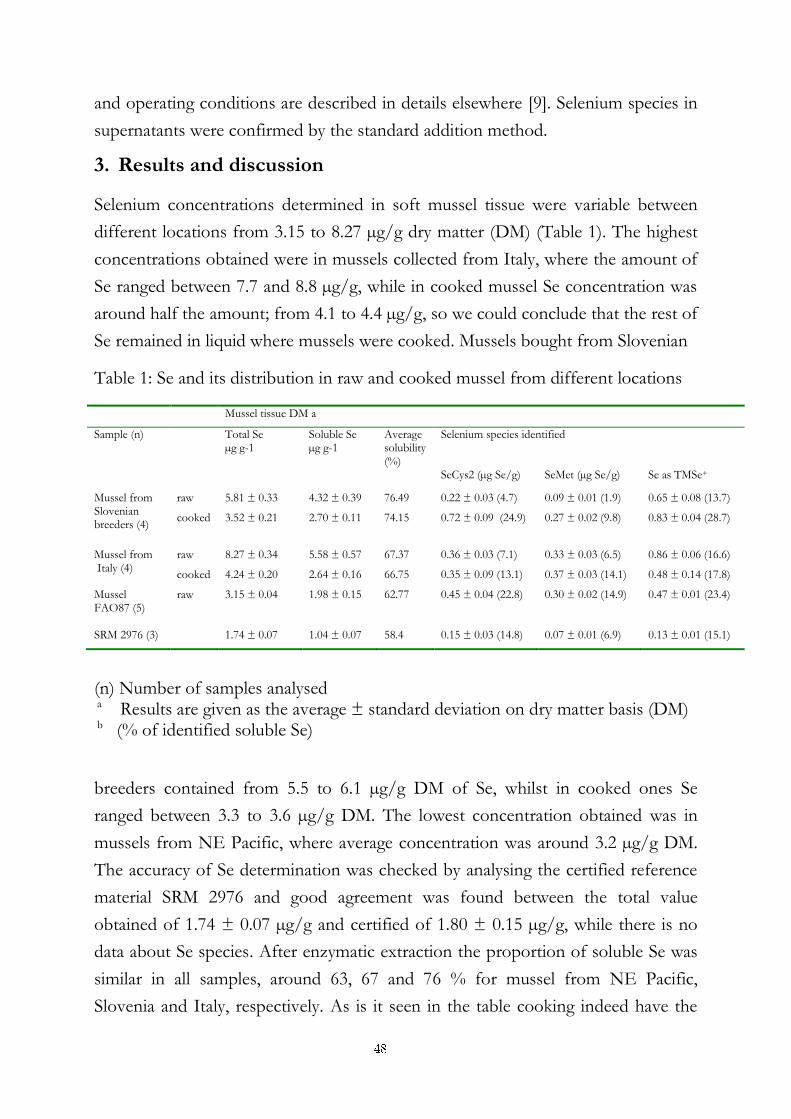
and operating conditions are described in details elsewhere [9]. Selenium species in
supernatants were confirmed by the standard addition method.
3. Results and discussion
Selenium concentrations determined in soft mussel tissue were variable between
different locations from 3.15 to 8.27 µg/g dry matter (DM) (Table 1). The highest
concentrations obtained were in mussels collected from Italy, where the amount of
Se ranged between 7.7 and 8.8 µg/g, while in cooked mussel Se concentration was
around half the amount; from 4.1 to 4.4 µg/g, so we could conclude that the rest of
Se remained in liquid where mussels were cooked. Mussels bought from Slovenian
Table 1: Se and its distribution in raw and cooked mussel from different locations
Mussel tissue DM a
Sample (n) Total Se µg g-1
Soluble Se µg g-1
Average solubility (%)
Selenium species identified
SeCys2 (µg Se/g) SeMet (µg Se/g) Se as TMSe+
Mussel from Slovenian breeders (4)
raw 5.81 ± 0.33 4.32 ± 0.39 76.49 0.22 ± 0.03 (4.7) 0.09 ± 0.01 (1.9) 0.65 ± 0.08 (13.7)
cooked 3.52 ± 0.21 2.70 ± 0.11 74.15 0.72 ± 0.09 (24.9) 0.27 ± 0.02 (9.8) 0.83 ± 0.04 (28.7)
Mussel from Italy (4)
raw 8.27 ± 0.34 5.58 ± 0.57 67.37 0.36 ± 0.03 (7.1) 0.33 ± 0.03 (6.5) 0.86 ± 0.06 (16.6)
cooked 4.24 ± 0.20 2.64 ± 0.16 66.75 0.35 ± 0.09 (13.1) 0.37 ± 0.03 (14.1) 0.48 ± 0.14 (17.8)
Mussel FAO87 (5)
raw 3.15 ± 0.04 1.98 ± 0.15 62.77 0.45 ± 0.04 (22.8) 0.30 ± 0.02 (14.9) 0.47 ± 0.01 (23.4)
SRM 2976 (3) 1.74 ± 0.07 1.04 ± 0.07 58.4 0.15 ± 0.03 (14.8) 0.07 ± 0.01 (6.9) 0.13 ± 0.01 (15.1)
(n) Number of samples analysed a Results are given as the average ± standard deviation on dry matter basis (DM) b (% of identified soluble Se)
breeders contained from 5.5 to 6.1 µg/g DM of Se, whilst in cooked ones Se
ranged between 3.3 to 3.6 µg/g DM. The lowest concentration obtained was in
mussels from NE Pacific, where average concentration was around 3.2 µg/g DM.
The accuracy of Se determination was checked by analysing the certified reference
material SRM 2976 and good agreement was found between the total value
obtained of 1.74 ± 0.07 µg/g and certified of 1.80 ± 0.15 µg/g, while there is no
data about Se species. After enzymatic extraction the proportion of soluble Se was
similar in all samples, around 63, 67 and 76 % for mussel from NE Pacific,
Slovenia and Italy, respectively. As is it seen in the table cooking indeed have the
48
effect on Se concentration since the amount of Se was almost half lower in cooked
mussels, nevertheless the percentage of Se solubility stayed the same. Liquid where
mussels from Italia were cooked was also analysed; the amount of Se was around
3.6 µg /g DM. Although a lot of Se stayed in liquid where mussels are cooked, we
need to take into account that by typical preparation of mussels liquid is also
included in the meal. In order to determine whether losses of selenium occur
during sample preparation (extraction and separation), a mass balance was drawn
up between the total selenium in the sample and the amount of selenium in the
supernatant and residue. The mass balance obtained for all mussel samples was
around 100 %, showing that there was no loss of Se. After enzymatic extraction,
chromatographic analysis of the supernatant was performed. Two selenium species
were identified and confirmed, SeCys2 and SeMet. In all chromatograms we
obtained one peak, which could not be identified due to the lack of Se standards.
We compared the peak with literature data, where authors identified TMSe+, and
found that the retention time on cationic column (with the same conditions as
ours) are the same, so we can conclude that the unknown Se species could be
TMSe+ [10].
References:
[1] M. Plessi, D. Bertelli, A. Monzani. Mercury and selenium content in selected seafood. Journal of Food Composition and Analysis, 14: 461-467, 2001
[2] M. Angeles Quijano, P. Moreno, A. M. Gutierrez, M. Concepcion Perez-Conde, C. Camara. Selenium speciation in animal tissues after enzymatic digestion by high-performance liquid chromatography coupled to inductively coupled plasma mass spectrometry. Journal of Mass Spectrometry, 35: 878-884, 2000
[3] German Nutrition Society (DGE), Austrian Nutrition Society (ÖGE), Swiss Society for Nutrition Research (SGE), Swiss Nutrition Association (SVE). Reference Values for Nutrient Intake, 1st ed. Druckerei V+V, Bonn, 2002.
[4] C. Thiry, A. Ruttens, L. De Temmerman, Y. J. Scheinder, L. Pussemier. Current knowledge in species-related bioavailability of selenium in food. Food Chemistry, 130: 767-784, 2012
[5] L. Hinojosa Reyes, J. L. Guzman Mar, G. M. Mizanur Rahman, B. Seybert, T. Fahrenholtz, H.M. Skip Kingston. Simultaneous determination of arsenic and selenium species in fish tissues using microwave-assisted enzymatic extraction and ion chromatography-inductively coupled plasma mass spectrometry. Talanta, 78: 983-990, 2009
[6] A. Osterc, T. Kanduč, Z. Šlejkovec, V. Stibilj, A. Ramšak. Mytilus Galloprovincialis as an indicator of environmental pollution along NE coast of Adriatic. In Proceedings of the tenth international conference on the Mediterranean coastal environment, MEDCOAST 11, Rhodes, Greece, 2011
[7] P. Smrkolj, V. Stibilj. Determination of selenium in vegetables by hydride generation atomic fluorescence spectrometry. Analytica Chimica Acta, 512: 11-17, 2004
[8] D. Mazej, I. Falnoga, M. Veber, V. Stibilj. Determination of selenium species in plant leaves by HPLC-UV-HG-AFS. Talanta, 68: 558-568, 2006
[9] P. Cuderman, I. Kreft, M. Germ, M. Kovačecič, V. Stibilj. Selenium species in selenium-enriched and drought exposed potatoes. Jornal of Agricultural and Food Chemistry, 56: 9114-9120, 2008
[10] P. Moreno, M. A. Quijano, A. M. Gutierrez, M. C. Perez-Conde, C. Camara. Fractionation studies of selenium compounds from oysters, and their determination by high-performance liquid chromatography coupled to inductively coupled plasma mass spectrometry. Journal of Analytical Atomic Spectrometry, 16: 1044-1050, 2001
49
For wider interest
Selenium (Se) is a complex, essential trace element for animal and human. It has
numerous important biological functions that depend on the activity of certain Se-
containing proteins. It is essential for the body because it forms seleno-enzymes
that carry out redox reactions such as glutathione peroxidase (GPx), thioredoxin
reductase, and thyroid hormone deiodinase families. However, Se is also considered
to be a toxic element at high concentrations. Function and bioavailability of this
element are strongly correlated with its chemical form, so it is necessary to control
the selenium intake to avoid deficiency diseases and toxicity problems. Therefore it
is important to determine the selenium species in foods, especially in seafood,
because of its known accumulation capacity. Our aim in this work was to
investigate selenium and its species with different analytical techniques in edible
mussel Mytilus galloprovincialis collected from different locations (Slovenian coastline,
Italy, Udine and NE Pacific). Furthermore we wanted to see if cooking of mussel
has any effect on selenium concentration and its distribution. In this experiment we
followed typical cooking procedure which is mostly used in Slovenia. To determine
total concentration of Se, hydride generation atomic fluorescence spectroscopy
(HG-AFS) was used. Total Se concentrations in mussels differ between the
locations where mussels were bred. The lowest concentrations obtained were in
mussel that comes from NE Pacific, but here we need to take into account that
mussels were already cleaned and removed from shell when we bought them from
the supermarket, while the mussels from Slovenia and Italy were cleaned in our
laboratory. Selenium speciation was performed by a liquid chromatography as
separation system and coupled to mass spectrometer as detector system (HPLC-
ICP-MS). Two selenium species were determined, while future work will involve
further species identification.
50
Research of innovative technologies for degasification of
lignite seam
Jerneja Lazar, Simon Zavšek, Sergej Jamnikar, Janja Žula, Gregor Uranjek,
Ludvik Golob
Premogovnik Velenje d.d., Partizanska 78, Velenje
Abstract. Gas outbursts are great problem in coal mines, especially in coal mining
of thick coal seams. In Velenje Coal mine up to 160 m thick coal seam presents a
large volume reservoir of coal gas. An average gas mixture ratio in Velenje coal gas
is approximately CO2:CH4 ≥ 2:1 from which high proportion of carbon dioxide is
adsorbed on lignite structure, while methane is free in coal fractures. “In-situ”
monitoring is provided in the mine with the support of laboratory analysis, such as
desorption and adsorption laboratory tests, and coupled numerical modelling of
gas migration under the influence of stress change is also performed. Individual
research work is focused on coupled geomechanical modelling of coal pillar.
Modelling is performed with two programs – Flac3D and TOUGH2. Different
models in Flac3D were prepared. Further on, the focus will be on the modelling of
gas pressure changes and gas migration around the borehole at the longwall Pesje
K. -50/C.
Keywords: gas outbursts, thick coal seam, coal gas, Flac3D modelling, TOUGH2
modelling
1 Introduction
Gas outbursts present high risk by the coal mining of thick coal seam, where thick
coal seam up to 160 m in Velenje Coal Mine presents a large volume reservoir for
coal gas and production of coal causes changes in stress and pore pressure around
the longwall coal face and coal gas can emit. When outburst occurs, the
rock/coal/gas system changed from a stable to an unstable state with the release of
a significant volume of gas over the duration of the outburst [1]. Outbursts with
CO2 are more violent, more difficult to control and more dangerous because of the
greater sorption capacity of carbon dioxide [2]. At Velenje Coal Mine, coal seam
51
has an average gas mixture ratio of approximately CO2:CH4 ≥ 2:1 with high
proportion of carbon dioxide which is adsorbed on lignite structure or it is
captured in the coals matrix and methane, which is free in coal fractures.
Coal gas concentrations has been monitored in various boreholes that were drilled
in coal pillars at different areas in coal mine. Also, coal gas pressure inside
boreholes has been measured under the influence of the retreating longwall coal
face. For determination of the detailed gas content, sorption (adsorption and
desorption) tests were performed on coal samples coupled with numerical
modelling of gas migration under the influence of stress change.
My individual research work mainly concerns the coupling geomechanical
modelling of coal pillar, which is under dynamic stresses of longwall top coal
caving. Modelling is performed with two programs – Flac3D and TOUGH2.
Numerical modelling is widely used in coal mining for understanding the behaviour
of coal under dynamic stresses. With coupling we will be able to understand how
the coal gas is migrating under dynamic stresses and how the gas migration is
influencing the gas outbursts. Flac3D is a three-dimensional explicit finite-
difference program for engineering mechanics computation. With the TOUGH2
we will be able to model behaviour of the coal gas under different permeability
changes. TOUGH2 is a general-purpose numerical simulator for multi-dimensional
fluid and heat flows of multiphase, multicomponent fluid mixtures in porous and
fractured media [3].
1.1 Coal geology
The Velenje coal seam is one of the thickest coal seams in the world and is located
in N Slovenia near the town Velenje. The lignite seam is lens-shaped with thickness
up to 165 m in the central part and the seam pinches out towards the margins and
lies in the Velenje basin. Under the lignite seam lays coal-bearing strata, which
consists of shales, clayey coal and lignite and is up to 50 m thick. The footwall lies
on more than 250 m thick green sandy silts. Above the coal seam, a thin layer of
marls with lacustrine molluscs was detected and after that thin layer is up to 350 m
thick lacustrine strata consisting of clays, marls and silts. This strata is overlain with
90 m thick sandy-silty formation. The most upper part of the basin consists of
terrestrial silts, overlain by recent fluvial sediments [4].
52
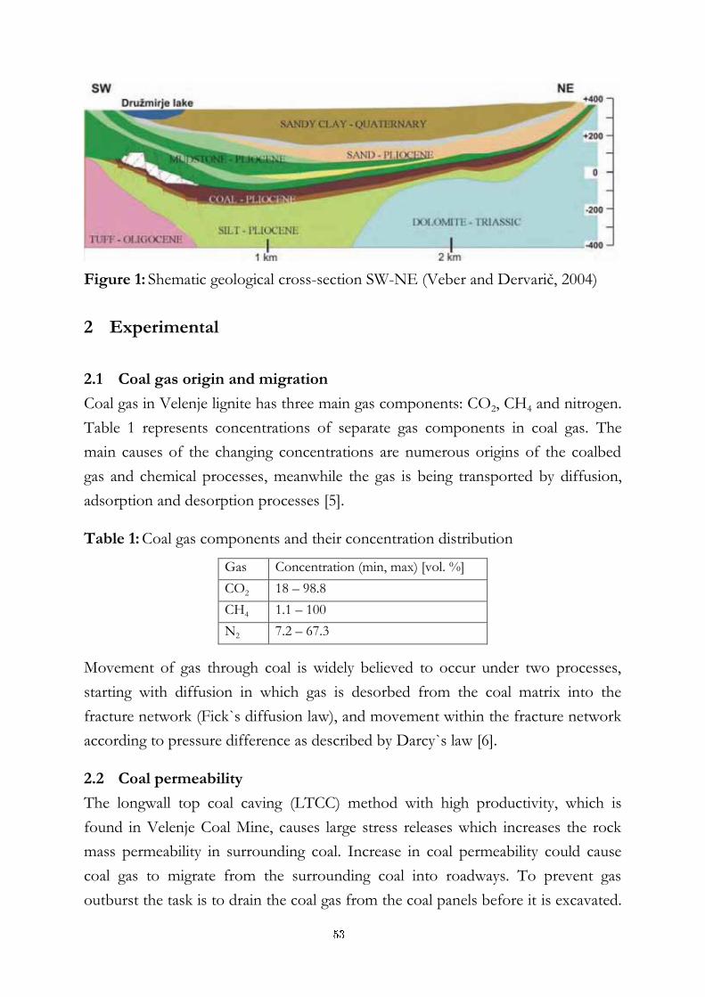
Figure 1: Shematic geological cross-section SW-NE (Veber and Dervarič, 2004)
2 Experimental
2.1 Coal gas origin and migration
Coal gas in Velenje lignite has three main gas components: CO2, CH4 and nitrogen.
Table 1 represents concentrations of separate gas components in coal gas. The
main causes of the changing concentrations are numerous origins of the coalbed
gas and chemical processes, meanwhile the gas is being transported by diffusion,
adsorption and desorption processes [5].
Table 1: Coal gas components and their concentration distribution
Gas Concentration (min, max) [vol. %]
CO2 18 – 98.8
CH4 1.1 – 100
N2 7.2 – 67.3
Movement of gas through coal is widely believed to occur under two processes,
starting with diffusion in which gas is desorbed from the coal matrix into the
fracture network (Fick`s diffusion law), and movement within the fracture network
according to pressure difference as described by Darcy`s law [6].
2.2 Coal permeability
The longwall top coal caving (LTCC) method with high productivity, which is
found in Velenje Coal Mine, causes large stress releases which increases the rock
mass permeability in surrounding coal. Increase in coal permeability could cause
coal gas to migrate from the surrounding coal into roadways. To prevent gas
outburst the task is to drain the coal gas from the coal panels before it is excavated.
53
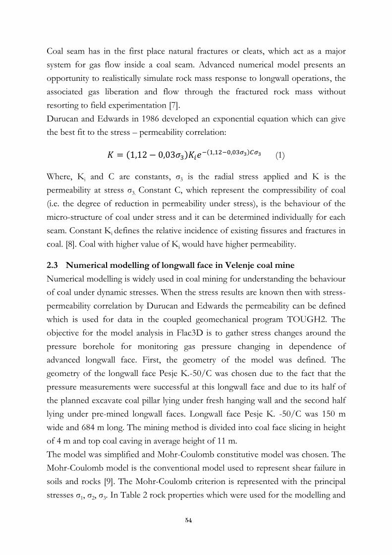
Coal seam has in the first place natural fractures or cleats, which act as a major
system for gas flow inside a coal seam. Advanced numerical model presents an
opportunity to realistically simulate rock mass response to longwall operations, the
associated gas liberation and flow through the fractured rock mass without
resorting to field experimentation [7].
Durucan and Edwards in 1986 developed an exponential equation which can give
the best fit to the stress – permeability correlation:
( ) ( ) (1)
Where, Ki and C are constants, σ3 is the radial stress applied and K is the
permeability at stress σ3. Constant C, which represent the compressibility of coal
(i.e. the degree of reduction in permeability under stress), is the behaviour of the
micro-structure of coal under stress and it can be determined individually for each
seam. Constant Ki defines the relative incidence of existing fissures and fractures in
coal. [8]. Coal with higher value of Ki would have higher permeability.
2.3 Numerical modelling of longwall face in Velenje coal mine
Numerical modelling is widely used in coal mining for understanding the behaviour
of coal under dynamic stresses. When the stress results are known then with stress-
permeability correlation by Durucan and Edwards the permeability can be defined
which is used for data in the coupled geomechanical program TOUGH2. The
objective for the model analysis in Flac3D is to gather stress changes around the
pressure borehole for monitoring gas pressure changing in dependence of
advanced longwall face. First, the geometry of the model was defined. The
geometry of the longwall face Pesje K.-50/C was chosen due to the fact that the
pressure measurements were successful at this longwall face and due to its half of
the planned excavate coal pillar lying under fresh hanging wall and the second half
lying under pre-mined longwall faces. Longwall face Pesje K. -50/C was 150 m
wide and 684 m long. The mining method is divided into coal face slicing in height
of 4 m and top coal caving in average height of 11 m.
The model was simplified and Mohr-Coulomb constitutive model was chosen. The
Mohr-Coulomb model is the conventional model used to represent shear failure in
soils and rocks [9]. The Mohr-Coulomb criterion is represented with the principal
stresses σ1, σ2, σ3. In Table 2 rock properties which were used for the modelling and
54
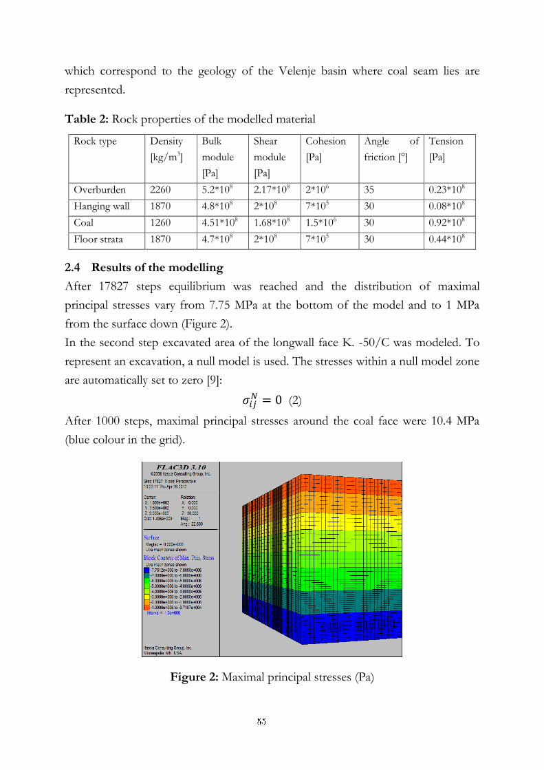
which correspond to the geology of the Velenje basin where coal seam lies are
represented.
Table 2: Rock properties of the modelled material
Rock type Density
[kg/m3]
Bulk
module
[Pa]
Shear
module
[Pa]
Cohesion
[Pa]
Angle of
friction [°]
Tension
[Pa]
Overburden 2260 5.2*108 2.17*108 2*106 35 0.23*108
Hanging wall 1870 4.8*108 2*108 7*105 30 0.08*108
Coal 1260 4.51*108 1.68*108 1.5*106 30 0.92*108
Floor strata 1870 4.7*108 2*108 7*105 30 0.44*108
2.4 Results of the modelling
After 17827 steps equilibrium was reached and the distribution of maximal
principal stresses vary from 7.75 MPa at the bottom of the model and to 1 MPa
from the surface down (Figure 2).
In the second step excavated area of the longwall face K. -50/C was modeled. To
represent an excavation, a null model is used. The stresses within a null model zone
are automatically set to zero [9]:
(2)
After 1000 steps, maximal principal stresses around the coal face were 10.4 MPa
(blue colour in the grid).
Figure 2: Maximal principal stresses (Pa)
55
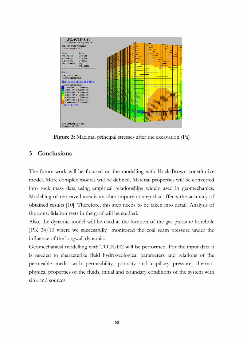
Figure 3: Maximal principal stresses after the excavation (Pa)
3 Conclusions
The future work will be focused on the modelling with Hoek-Brown constitutive
model. More complex models will be defined. Material properties will be converted
into rock mass data using empirical relationships widely used in geomechanics.
Modelling of the caved area is another important step that affects the accuracy of
obtained results [10]. Therefore, this step needs to be taken into detail. Analysis of
the consolidation tests in the goaf will be studied.
Also, the dynamic model will be used at the location of the gas pressure borehole
JPK 34/10 where we successfully monitored the coal seam pressure under the
influence of the longwall dynamic.
Geomechanical modelling with TOUGH2 will be performed. For the input data it
is needed to characterize fluid hydrogeological parameters and relations of the
permeable media with permeability, porosity and capillary pressure, thermo-
physical properties of the fluids, initial and boundary conditions of the system with
sink and sources.
56
4 References
[1] Choi, X. and Wold, M., Study of the Mechanism of Coal and Gas Outbursts Using a New
Numerical Modeling Approach ,2004. Underground Coal Operators´ Conference. Paper 142.
[2] Lama, R. and Saghafi, A., Overview of Gas Outbursts and Unusual Emissions, 2002.
Underground Coal Operators´ Conference. Paper 196.
[3] Prues, K., Oldenburg, C. and Moridis, G., TOUGH2 User`s Guide, Version 2.0, 1999. Ernest
Orlando Lawrence Berkeley National Laboratory.
[4] Kanduc, T., Pezdic, J., Origin and distribution of coalbed gases from the Velenje basin,
Slovenia, 2005. Geochemical Journal, Vol.39.
[5] Pezdič, J., Markič, M., Letič, M., Popovič, A., Zavšek, S., Laboratory simulation of desorption
– desorption processes on different lignite lithotypes from Velenje lignite mine,1999, RMZ –
Materials and Geoenviroment, Vol. 46, No. 3, 555-568, Paper.
[6] Williams, R.J. and Weissman, J.J., Gas emission and outburst assessment in mixed CO2 and
CH4 environments, 1995. ACIRL Undeground Mining Seminar Brisbane, Paper.
[7] Esterhuinzen, G.S., Karacan, C.O., Development of Numerical Models to Investigate
Permeability Changes and Gas Emissions around Longwall Mining Panel, paper.
[8] Durucan, S. and Edwards, J.S., The Effects of Stress and Fracturing on Permeability of Coal,
1986. Mining Science and Technology, 3, 205-216. Paper.
[9] Itasca, Flac3D: Fast Lagrangian Analysis of Continua in 3 Dimensions, Online Manual.
[10] Yatsili, N.E., and Unver, B., 3-D numerical modelling of stresses around a longwall panel
with top coal caving, 2005. The Journal of The South African Institute of Mining and Metallurgy, Paper.
57

For wider interest
In the last few years the importance of coal as an energy source is raising again, due
to development of Clean Coal Technologies (CCT). However, coal combustion
produces billions of tonnes of carbon dioxide each year and all of that is released to
the atmosphere. Because of the problems with greenhouse gas emissions at Velenje
Coal Mine we launched a research group on Clean Coal Technologies (at the end of
year 2007). The task of the research group is to find new technologies for cleaner
use of coal. Clean Coal Technologies research group also applied for two
international projects. First is Development of Novel Technologies for Predicting
and Combating Gas Outbursts and Uncontrolled Emissions in Thick Seam Coal
Mining, which will improve coal excavation, safety and working conditions in the
mine (CoGasOUT). The project is partially founded by Research Fund for Coal
and Steel. The second project entitled Greenhouse Gas Recovery from Coal mines
and Coalbeds for Conversion to Energy (GHG2E) is funded within the 7th
framework programme. During both projects, “in-situ” monitoring is provided in
the mine with the support of laboratory analysis, such as desorption and adsorption
laboratory tests, coupled with numerical modelling of gas migration under the
influence of stress change. Results will improve mines around the world with new
technology to combat outbursts and high gas emissions.
58
Use of monolithic chromatography for speciation of Pt based chemotherapeutic drugs
Anže Martinčič1,2, Radmila Milačič1,2, Maja Čemažar3, Gregor Serša3, and
Janez Ščančar1,2
1 Department of Environmental sciences, Jožef Stefan Institute, Ljubljana, Slovenia
2 Jožef Stefan International Postgraduate School, Ljubljana, Slovenia
3 Institute of Oncology, Department of Experimental Oncology, Ljubljana, Slovenia
Abstract. Distribution of Pt-based chemo-therapeutic drugs; cisplatin, carboplatin
and oxaliplatin was studied using monolithic chromatography coupled to inductively
coupled plasma mass spectrometry (ICP-MS). Previously developed method for
speciation of cisplatin was successfully used for pharmacokinetic studies of
oxaliplatin and carboplatin in human serum.
Keywords: cisplatin, carboplatin, oxaliplatin, monolithic chromatography, ICP-MS
1 Introduction
Pt-based chemotherapeutic drugs: cisplatin (CDDP), carboplatin and oxaliplatin, are
applied worldwide in clinical practice. [1] The cytotoxicity of these drugs is a consequence
of Pt’s binding to DNA which results in cellular death by apoptosis or necrosis. [2]
CDDP is used for treating numerous types of tumours (testicular, ovarian, cervical,
bladder, etc.) but its use is limited by severe side effects. [2] Carboplatin exhibits fewer
side effects but is also less effective than CDDP. It is mainly used to treat ovarian
carcinoma, lung, head and neck cancers. [3] Oxaliplatin was approved in 1996 and is
mainly used to treat colorectal cancer.
Analytical chemistry is today essentially involved in research in life sciences. Inductively
coupled plasma mass spectrometry (ICP-MS) is an elemental MS technique characterized
by its isotope specificity, versatility, high sensitivity, large linear dynamic range and
robustness. Coupled to high pressure liquid chromatography (HPLC) it is the method of
choice for speciation analysis. [4] In our previous work an analytical method for
speciation of CDDP in human blood serum was developed. [5] In this paper we present
59
the applicability of the developed method for studying pharmacokinetics of other Pt
based chemotherapeutic drugs.
1.1 Materials and methods
HPLC separations were performed with an Agilent (Tokyo, Japan) series 1200 quaternary
system on a weak anion-exchange CIM DEAE-1 monolithic column (Bia Separations,
Ljubljana, Slovenia). Protein signals were followed online with UV-Vis detector at 278
nm and 195Pt signals with Agilent 7700x ICP-MS.
The chromatographic run was carried out at a flow rate of 1 mL min-1. Linear gradient
elution from 100% buffer A (50 mM TRIS HCl + 30 mM HCO3- at pH 7.4) to 100%
buffer B (buffer A + 1 M NH4Cl) was applied for 10.5 min. The column was then
regenerated by rinsing with 100% buffer C (2 M NH4Cl) for 2 min at flow rate 10 mL
min-1, followed by elution with buffer D (0.2 M TRIS HCl at pH 7.4) for 3 min at flow
rate 10 mL min-1. After that, the column was equilibrated with buffer A at a flow rate of
10 mL min-1 for 2 min and at flow rate of 1 mL min-1 from 17.5 to 19.5 min.
Human serum was spiked with the equivalent of 200 ng Pt mL-1 of each drug separately
and incubated for 24 h at 37 °C. For kinetic studies human serum was first warmed to 37
°C and than spiked with the equivalent of 200 ng Pt mL-1 of each drug. 0.1 mL of serum
was taken for speciation analysis at 5 min, 1 h, 3 h, 5 h, 24 h and 48 h. Before analysis
each sample was diluted five times with buffer A.
1.2 Results
In our previous work we showed that the main binding site for CDDP in human serum
was human serum albumin (HSA) on to which 83 % of all CDDP was bound while 3 %
of all CDDP was bound to transferrin (Tf) and 14 % remained unbound (Fig.1).
Unbound drug elutes at the retention volume of immunoglobulins (IgG), but it was
shown that it is not bound to IgG. [5] Molar ratio of HSA/Tf is ~10/1 while Pt ratio
between them is ~28/1. We found that oxaliplatin behaves similarly to CDDP; 63 % of
all oxaliplatin was bound to HSA, 10 % was bound to Tf and 27 % remained unbound.
Carboplatin on the other hand remains predominantly unbound (74.5 %) and only 7.5 %
was bound to Tf and 18 % to HSA.
Kinetics of binding to human serum proteins was also studied. Results show that CDDP
and oxaliplatin bind quickly to serum proteins. (Fig. 2) After only 3 h most of CDDP and
60
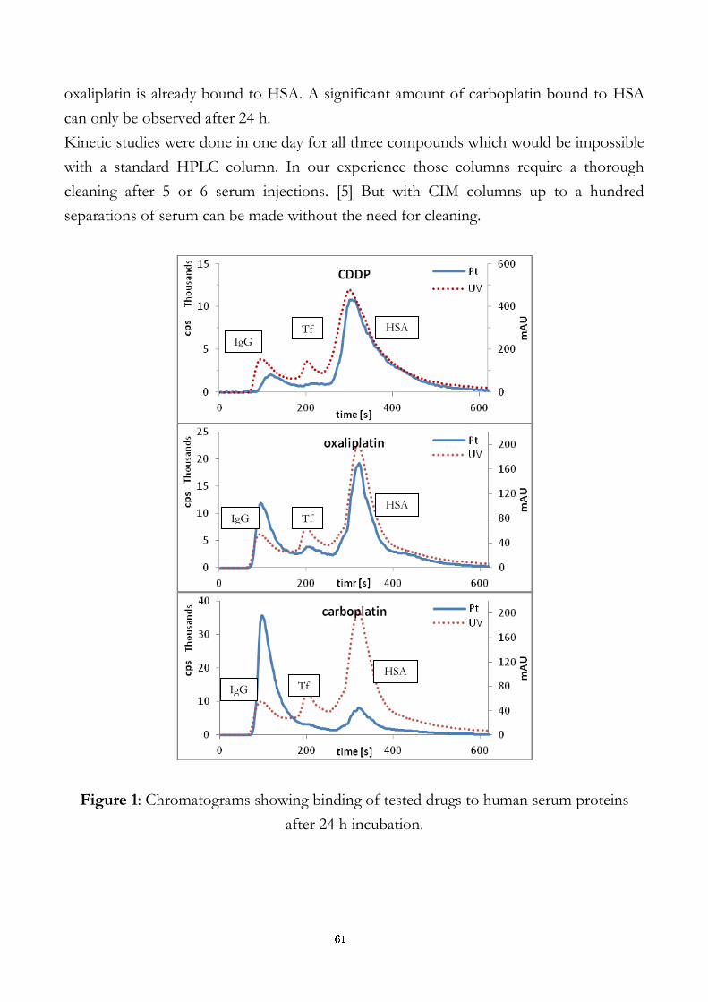
oxaliplatin is already bound to HSA. A significant amount of carboplatin bound to HSA
can only be observed after 24 h.
Kinetic studies were done in one day for all three compounds which would be impossible
with a standard HPLC column. In our experience those columns require a thorough
cleaning after 5 or 6 serum injections. [5] But with CIM columns up to a hundred
separations of serum can be made without the need for cleaning.
Figure 1: Chromatograms showing binding of tested drugs to human serum proteins
after 24 h incubation.
Tf
HSA
IgG
Tf HSA
IgG
HSA
Tf IgG
61
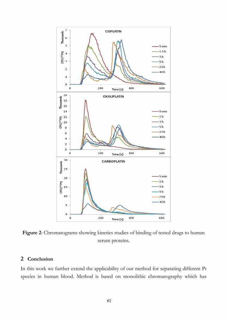
Figure 2: Chromatograms showing kinetics studies of binding of tested drugs to human
serum proteins.
2 Conclusion
In this work we further extend the applicability of our method for separating different Pt
species in human blood. Method is based on monolithic chromatography which has
62

several advantages over standard (particle packed) chromatographic columns. In our
future work will further develop this method for speciation of Ru-based compounds.
References:
[1] F. Huq, J. Q. Yu, P. Beale, in A. Boneti, R. Leone, F. M. Muggia, S. B. Howell (ed.), Platinum and Other Heavy Metal Compounds in Cancer Chemotherapy, Humana Press Inc., New York, 2009.
[2] D. Esteban-Fernandez, E. Moreno-Gordaliza, B. Canas, M. A. Palacios and M. M. Gomez-Gomez, Metallomics, 2, 19–38, 2010.
[3] NJ. Wheate, S. Walker, GE. Craig, R. Oun., Dalton Trans, 39, 8113-27, 2010.
[4] D. M. Templeton, F. Ariese, R. Cornelis, L.-G. Danielsson, H. Muntau, H. P. Van Leeuwen and R. Lobinski, Pure Appl. Chem., 72, 1453–1470, 2000.
[5] A. Martinčič, R. Milačič, M. Čemažar, G. Serša, J. Ščančar, Anal. Methods, 4, 780-790, 2012.
63

For wider interest
Our work is based on monolithic chromatography which offers several advantages over
standard (particle packed) chromatographic columns. Monolithic supports have high
permeability and therefore allow thorough cleaning during regeneration after each
separation run. This enables great robustness of such chromatographic columns which in
turn enables higher throughput of samples. Monolithic supports are also cheaper and
offer possibilities to be applied in numerous chromatographic separations of compounds
in environmental and biological samples.
64
Determnation of Cr(VI) in corrosion protection coatings by
speciated isotope dilution ICP-MS
Breda Novotnik1,2, Tea Zuliani1, Janez Ščančar1,2 and Radmila Milačič1,2
1 Department of Environmental sciences, Jožef Stefan Institute, Ljubljana, Slovenia
2 Jožef Stefan International Postgraduate School, Ljubljana, Slovenia
Abstract: Chromium conversion coatings are used as decorative finishes and to
improve the corrosion protection and strengthen the wear resistance of metallic
surfaces. Chromium electroplating frequently involves the use of hexavalent
chromium (Cr). To reduce environmental impacts, several EU directives restricted
its use to threshold values of 0.1 % Cr(VI) by weight per homogenous material in
vehicles, and 1000 mg kg-1 of Cr(VI) in electronic and electrical equipment. In a
view of these demands the aim of our work was to develop a selective and
quantitative analytical procedure for determination of Cr(VI) in corrosion protection
coatings. The results have proven that for efficient extraction of Cr(VI), 2 % NaOH
+ 3 % Na2CO3 with addition of MgCl2 as extraction solution and ultrasonic
extraction at 70 °C for 30 min should be applied. Several consecutive extractions are
necessary to quantitatively extract Cr(VI) from corrosion prevention coatings.
Key words: corrosion protection coatings, chromium(VI), speciated isotope
dilution, Inductively Coupled Plasma Mass Spectrometry
1 Introduction
The amount of Cr(VI) in corrosion protection coatings and electrical equipment is
of environmental concern and is restricted by several legislation directives [1-3]. To
date, determination of Cr(VI) in corrosion protection coatings was mainly
performed by hot water extraction and spectrophotometric 1,5 diphenylcharbazide
detection (EN 15205, [4]) or by the use of slightly alkaline ammonia extracting
solution (pH 9) and quantification of Cr(VI) by HPLC-ICP-MS [5]. Since hot water
and alkaline buffers with low ionic strength are not powerful leaching agents, the
aim of our work was to develop a method based on alkaline extraction, that would
enable selective and quantitative determination of Cr(VI) in corrosion protection
coatings. Species interconversions during the extraction procedure were followed
65
by the use of stable isotopes. Cr(VI) was quantified by isotope dilution inductively
coupled plasma mass spectrometry (ID-FPLC-ICP-MS) procedure.
2 Materials and methods
Preparation of enriched isotopic standard solutions 50Cr(VI) standard solution was prepared by alkaline melting from Cr2O3 (50Cr
enriched isotope). 53Cr(III) standard solution was prepared from Cr2O3 (53Cr
enriched isotope) by microwave assisted digestion. Determination of the
concentrations of enriched 53Cr(III) and 50Cr(VI) standard solutions was performed
by reverse ID-ICP-MS. A dead time of 46 ns was used. The mass bias was
determined daily by chromatographic separation of natCr(VI) at concentrations that
were close to Cr concentrations in the samples investigated.
Sample preparation
Chromium conversion or hard chrome coatings on electroplated copper (10 µm) or
zinc (10 µm) steel surfaces (metallic plates 10 mm x 10 mm x 1.5 mm) of 5 or 10
µm thickness of homogenously coated chromium layer were prepared in a
galvanization workshop.
Extraction procedure
A final volume of 10 mL of extraction solution was prepared from 2 % NaOH+3
% Na2CO3, 1 mL of MgCl2 (1 mol L-1) and enriched isotopic spike solutions of 50Cr(VI) and 53Cr(III) (20 ng Cr mL-1). Ultrasonic extraction was applied at 70 °C
for 30 min. Six consecutive extractions were performed. Analysis of Cr(VI) in
extracts was performed by high performance liquid chromatography HPLC-ICP-
MS. Concentrations of Cr(VI) were calculated by speciated isotope dilution ICP-
MS, based on determining the signal intensities ratio between 50Cr(VI) enriched
spike and 52Cr(VI) present in the sample (RVI50/52 ratio).
3 Results and discussion
Optimisation of the extraction procedure
To check whether any oxidation and/or reduction occurs during the extraction of
chromium from plates, a double isotopically enriched spike of 50Cr(VI) and 53Cr(III) was added to extracting solution. As can be seen from Fig. 1A, noticeable
66
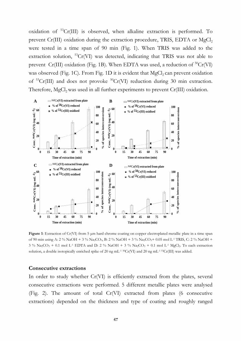
oxidation of 53Cr(III) is observed, when alkaline extraction is performed. To
prevent Cr(III) oxidation during the extraction procedure, TRIS, EDTA or MgCl2
were tested in a time span of 90 min (Fig. 1). When TRIS was added to the
extraction solution, 53Cr(VI) was detected, indicating that TRIS was not able to
prevent Cr(III) oxidation (Fig. 1B). When EDTA was used, a reduction of 50Cr(VI)
was observed (Fig. 1C). From Fig. 1D it is evident that MgCl2 can prevent oxidation
of 53Cr(III) and does not provoke 50Cr(VI) reduction during 30 min extraction.
Therefore, MgCl2 was used in all further experiments to prevent Cr(III) oxidation.
A B
C D
0 15 30 45 60 75 900
20
40
60
natCr(VI) extracted from plate
% of 50Cr(VI) reduced
% of 53Cr(III) oxidised
Time of extraction (min)
Con
c. n
at C
r(V
I)
(ng m
L-1
)
0
20
40
60
80
100
% o
f sp
ecie
s i
nte
rcon
versio
n
0 15 30 45 60 75 900
20
40
60
natCr(VI) extracted from plate
% of 50Cr(VI) reduced
% of 53Cr(III) oxidised
Time of extraction (min)
Con
c. n
at C
r(V
I)
(ng m
L-1
)
0
20
40
60
80
100
% o
f sp
ecie
s i
nte
rcon
versio
n
0 15 30 45 60 75 900
20
40
60
Con
c. n
at C
r(V
I)
(ng m
L-1
)
Time of extraction (min)
natCr(VI) extracted from plate
% of 50Cr(VI) reduced
% of 53Cr(III) oxidised
0
20
40
60
80
100
% o
f sp
ecie
s i
nte
rcon
versio
n
0 15 30 45 60 75 900
20
40
60
Time of extraction (min)
natCr(VI) extracted from plate
% of 50Cr(VI) reduced
% of 53Cr(III) oxidised
0
20
40
60
80
100
Con
c. n
at C
r(V
I)
(ng m
L-1
)
% o
f sp
ecie
s i
nte
rcon
versio
n
Figure 1: Extraction of Cr(VI) from 5 μm hard chrome coating on copper electroplated metallic plate in a time span
of 90 min using A: 2 % NaOH + 3 % Na2CO3, B: 2 % NaOH + 3 % Na2CO3+ 0.05 mol L-1 TRIS, C: 2 % NaOH +
3 % Na2CO3 + 0.1 mol L-1 EDTA and D: 2 % NaOH + 3 % Na2CO3 + 0.1 mol L-1 MgCl2. To each extraction
solution, a double isotopically enriched spike of 20 ng mL-1 50Cr(VI) and 20 ng mL-1 53Cr(III) was added.
Consecutive extractions
In order to study whether Cr(VI) is efficiently extracted from the plates, several
consecutive extractions were performed. 5 different metallic plates were analysed
(Fig. 2). The amount of total Cr(VI) extracted from plates (6 consecutive
extractions) depended on the thickness and type of coating and roughly ranged
67
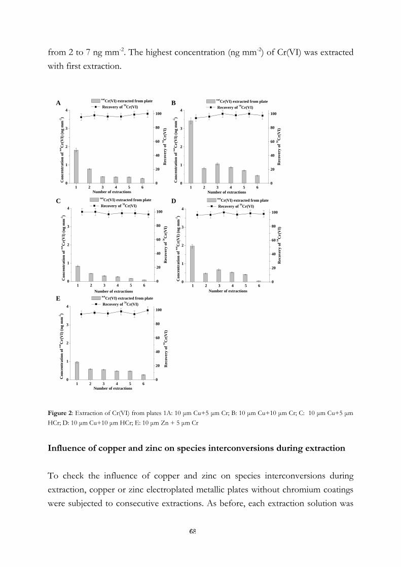
from 2 to 7 ng mm-2. The highest concentration (ng mm-2) of Cr(VI) was extracted
with first extraction.
A B
C D
E
1 2 3 4 5 60
1
2
3
4
nat
Cr(VI) extracted from plate
Recovery of 50
Cr(VI)
Number of extractions
Con
cen
trati
on
of
nat C
r(V
I) (
ng m
m-2)
0
20
40
60
80
100
Recovery o
f 50C
r(V
I)
1 2 3 4 5 60
1
2
3
4
Number of extractions
nat
Cr(VI) extracted from plate
Recovery of 50
Cr(VI)
Con
cen
trati
on
of
nat C
r(V
I) (
ng m
m-2)
0
20
40
60
80
100
Recovery o
f 50C
r(V
I)
1 2 3 4 5 60
1
2
3
4
nat
Cr(VI) extracted from plate
Recovery of 50
Cr(VI)
Number of extractions
Con
cen
trati
on
of
nat C
r(V
I) (
ng m
m-2)
0
20
40
60
80
100
Recovery o
f 50C
r(V
I)
1 2 3 4 5 60
1
2
3
4
nat
Cr(VI) extracted from plate
Recovery of 50
Cr(VI)
Number of extractions
Con
cen
trati
on
of
na
t Cr(V
I) (
ng m
m-2)
0
20
40
60
80
100
Recovery o
f 50C
r(V
I)
1 2 3 4 5 60
1
2
3
4
nat
Cr(VI) extracted from plate
Recovery of 50
Cr(VI)
Number of extractions
Con
cen
trati
on
of
nat C
r(V
I) (
ng m
m-2)
0
20
40
60
80
100
Recovery o
f 50C
r(V
I)
Figure 2: Extraction of Cr(VI) from plates 1A: 10 μm Cu+5 μm Cr; B: 10 μm Cu+10 μm Cr; C: 10 μm Cu+5 μm
HCr; D: 10 μm Cu+10 μm HCr; E: 10 μm Zn + 5 μm Cr
Influence of copper and zinc on species interconversions during extraction
To check the influence of copper and zinc on species interconversions during
extraction, copper or zinc electroplated metallic plates without chromium coatings
were subjected to consecutive extractions. As before, each extraction solution was
68
spiked with isotopically enriched 50Cr(VI) and 53Cr(III). This experimental data
proved that no oxidation of 53Cr(III) occurred during consecutive extractions. 50Cr(VI) was not reduced during consecutive extractions from copper electroplated
metallic plates, but significant reduction of 50Cr(VI) was observed after the first
extraction from zinc electroplated plates. Meaning that zinc in the following
extractions acted as a reducing agent. From the analytical point of view, this means
that any mechanical damage to the chromium coatings on electroplated zinc
surfaces may consequently cause the reduction of Cr(VI) during extraction.
In conclusion, 30 min ultrasonic extraction at 70 °C using 2 % NaOH + 3 %
Na2CO3 + MgCl2 as extracting agent and 6 consecutive extractions were necessary
to quantitatively extract Cr(VI) from protective layers. The use of enriched isotopic
solutions of 50Cr(VI) and 53Cr(III) enabled to control species interconverstions
during the analytical procedure and to quantify Cr(VI) by speciatied ID-ICP-MS.
However, once the analytical procedure was optimised, quantification of Cr(VI) is
also possible by ICP-MS, using external calibration. The method developed is
highly sensitive. Limit of quantification (LOQ) was found to be 0.0107 ng Cr(VI)
mm-2 if the coating surface was 250 mm2. The possibility to use external calibration
for quantification of separated Cr(VI) instead of ID-ICP-MS, extends the
application of the developed procedure to routine laboratory use.
References
[1.] The Council of the European Union, 2000, European Directive 2000/53/EC on end-of life
vehicles. Official Journal of European Union
[2.] The Council of the European Union, 2002, European Directive 2002/95/EC on the
restriction of the use of certain hazardous substances in electrical and electronic equipment.
Official Journal of European Union
[3.] The Council of the European Union, 2002, European Directive 2002/96/EC on waste
electrical and electronic equipment (WEEE). Official Journal of European Union
[4.] ISO (1995) EN ISO 3613. ISO, Geneva
[5.] F. Séby, A. Castetbon, R. Ortega, C. Guimon, F. Niveau, N. Barrois-Oudin, H. Garraud and
O.F.X. Donard. Development of analytical procedures for the determination of hexavalent
chromium in corrosion prevention coatings used in the automotive industry. Analitical and
Bioanalitical Chemistry,391: 587-597, 2008
69
Za širši interes
Evropska unija je sprejela številne predpise s katerimi določa kritične meje
Cr(VI) v protikorozijskih premazih, ki se uporabljajo v avtomobilski industriji
(2000/53/EC) in elektronski opremi (2002/95/EC) ter v recikliranih izdelkih
(2002/96/EC). Postopki, ki so trenutno v uporabi za analizo Cr(VI) vključujejo
ekstrakcijo z vrelo vodo ali rahlo alkalno amonijevo raztopino, ter
spektrofotometrično določitev Cr(VI) v ekstraktu oziroma določitev z ICP-MS.
Ker omenjeni ekstrakcijski sredstvi nista dovolj učinkoviti, je bil naš cilj razviti
novo analizno metodo, ki temelji na alkalni ekstrakciji. Pri razvoju
ekstrakcijskega postopka smo uporabili stabilne izotope kroma (50Cr(VI) in
53Cr(III)) s katerimi smo sledili oksidaciji in redukciji kromovih zvrsti med
samim ekstrakcijskih postopkom. Ugotovili smo, da alkalna ekstrakcija povzroči
oksidacijo Cr(III) v vzorčku. Da bi preprečili oksidacijo kroma med ekstrakcijo,
smo preverili v kakšni meri TRIS, EDTA in MgCl2 preprečijo oksidacijo Cr(III).
Poskusi so pokazali, da TRIS ni sposoben preprečiti oksidacije in, da se pri
dodatku EDTA pojavi redukcija Cr(VI). MgCl2 se je tako izkazal kot
najustreznejši, saj pri 30 min ekstrakcije nismo zasledili oksidacije Cr(III) ali
redukcije Cr(VI). Tako smo v vseh nadaljnjih poskusih za ekstrakcijo Cr(VI)
uporabili ultrazvočno ekstrakcijo (30 min, 70 °C) in kot ekstrakcijsko sredstvo 2
% NaOH + 3 % Na2CO3 z dodatkom MgCl2. Omenjeni postopek ekstrakcije je
zagotovil pogoje, pri katerih ni prišlo do pretvorb kromovih zvrsti, kar smo
dodatno sledili med vsako ekstrakcijo z uporabo obogatenih stabilnih izotopov
kroma 50Cr(VI) in 53Cr(III). Cr(VI) v ekstraktu smo določili z izredno
občutljivo kvantitativno metodo izotopskega redčenja z ICP-MS. Ugotovili smo,
da je bilo pri preučevanih vzorcih za ekstrakcijo celotnega Cr(VI) iz površine
nanosa protikorozijskih prevlek potrebnih šest zaporednih ekstrakcij.
70
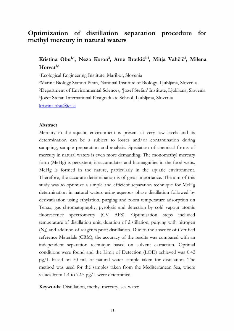
Optimization of distillation separation procedure for methyl mercury in natural waters
Kristina Obu1,4, Neža Koron2, Arne Bratkič3,4, Mitja Vahčič3, Milena
Horvat3,4
1Ecological Engineering Institute, Maribor, Slovenia
2Marine Biology Station Piran, National Institute of Biology, Ljubljana, Slovenia
3Department of Environmental Sciences, ‘Jozef Stefan’ Institute, Ljubljana, Slovenia
4Jožef Stefan International Postgraduate School, Ljubljana, Slovenia
Abstract
Mercury in the aquatic environment is present at very low levels and its
determination can be a subject to losses and/or contamination during
sampling, sample preparation and analysis. Speciation of chemical forms of
mercury in natural waters is even more demanding. The monomethyl mercury
form (MeHg) is persistent, it accumulates and biomagnifies in the food webs.
MeHg is formed in the nature, particularly in the aquatic environment.
Therefore, the accurate determination is of great importance. The aim of this
study was to optimize a simple and efficient separation technique for MeHg
determination in natural waters using aqueous phase distillation followed by
derivatisation using ethylation, purging and room temperature adsorption on
Tenax, gas chromatography, pyrolysis and detection by cold vapour atomic
fluorescence spectrometry (CV AFS). Optimisation steps included
temperature of distillation unit, duration of distillation, purging with nitrogen
(N2) and addition of reagents prior distillation. Due to the absence of Certified
reference Materials (CRM), the accuracy of the results was compared with an
independent separation technique based on solvent extraction. Optimal
conditions were found and the Limit of Detection (LOD) achieved was 0.42
pg/L based on 50 mL of natural water sample taken for distillation. The
method was used for the samples taken from the Mediterranean Sea, where
values from 1.4 to 72.5 pg/L were determined.
Keywords: Distillation, methyl mercury, sea water
71
1 Introduction
Mercury (Hg) is a toxic metal for humans and the ecosystem. It is a natural
element, but during the last century of human activities increased its presence in the
global atmosphere for about a factor of three [1, 2]. The main anthropogenic
activities include burning of fossils fuels, high temperature processes (ore, metal
industry, cement kilns) and the use of mercury in industrial processes and products
[3]. In the environment different forms of mercury (elementary Hg0, inorganic Hg2+
and Hg22+, organic MeHg) are present, of which elemental Hg is volatile at room
temperature. Transformation of these forms under natural conditions form the
basis for the local, regional and global biogeochemical cycle. Due to its volatile
nature it can travel long distances and can be deposited far from its source and it is
therefore characterized as a global pollutant. Oceans play very important role in
the global mercury cycle. Due to reduction/oxidation processes oceans can be a
source and/or sink of mercury from the global atmosphere. In the water and
sediments mercury can be transformed to MeHg, which is one of the most toxic
Hg compound and accumulates and biomagnifies in the aquatic food webs.
Therefore, it is of paramount importance to obtain accurate information about the
presence and formation of this compound in the aquatic environment [3].
The concentrations of mercury in natural waters are low, and range from 0.2 to a
few ng/L. In natural waters, especially in sea water, MeHg occurs in very low
concentrations; typically, less than 10 % of total Hg in water exists as MeHg [3].
The analysis is therefore demanding and can be a subject to losses and/or
contamination during sampling, sample handling and analysis. For the purpose of
MeHg isolation from the matrix, two methods are commonly used. The first is
based on extraction procedure using organic solvents (methylene chloride) and the
second is based on aqueous phase distillation [1]. Both methods are followed by a
derivatisation procedure and CV AFS detection [1] which is sensitive enough to
measure sub picogram levels of MeHg. Although the distillation technique has been
in use for a long time [1], it is very important to optimize the procedure to achieve
required precision, good recoveries and contamination-free conditions. In order to
achieve suitable LOD, the procedure should be simple, involving limited number
of steps, and reagents. The aim of this work was to optimize the distillation
72
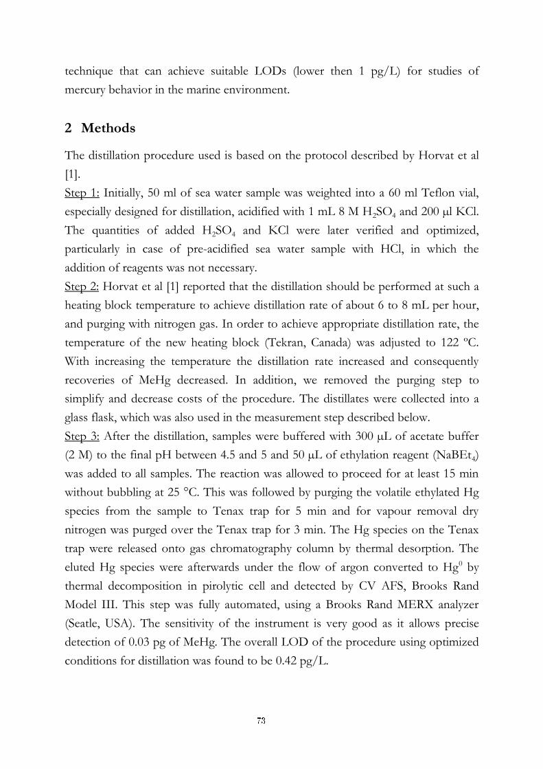
technique that can achieve suitable LODs (lower then 1 pg/L) for studies of
mercury behavior in the marine environment.
2 Methods
The distillation procedure used is based on the protocol described by Horvat et al
[1].
Step 1: Initially, 50 ml of sea water sample was weighted into a 60 ml Teflon vial,
especially designed for distillation, acidified with 1 mL 8 M H2SO4 and 200 µl KCl.
The quantities of added H2SO4 and KCl were later verified and optimized,
particularly in case of pre-acidified sea water sample with HCl, in which the
addition of reagents was not necessary.
Step 2: Horvat et al [1] reported that the distillation should be performed at such a
heating block temperature to achieve distillation rate of about 6 to 8 mL per hour,
and purging with nitrogen gas. In order to achieve appropriate distillation rate, the
temperature of the new heating block (Tekran, Canada) was adjusted to 122 ºC.
With increasing the temperature the distillation rate increased and consequently
recoveries of MeHg decreased. In addition, we removed the purging step to
simplify and decrease costs of the procedure. The distillates were collected into a
glass flask, which was also used in the measurement step described below.
Step 3: After the distillation, samples were buffered with 300 µL of acetate buffer
(2 M) to the final pH between 4.5 and 5 and 50 µL of ethylation reagent (NaBEt4)
was added to all samples. The reaction was allowed to proceed for at least 15 min
without bubbling at 25 °C. This was followed by purging the volatile ethylated Hg
species from the sample to Tenax trap for 5 min and for vapour removal dry
nitrogen was purged over the Tenax trap for 3 min. The Hg species on the Tenax
trap were released onto gas chromatography column by thermal desorption. The
eluted Hg species were afterwards under the flow of argon converted to Hg0 by
thermal decomposition in pirolytic cell and detected by CV AFS, Brooks Rand
Model III. This step was fully automated, using a Brooks Rand MERX analyzer
(Seatle, USA). The sensitivity of the instrument is very good as it allows precise
detection of 0.03 pg of MeHg. The overall LOD of the procedure using optimized
conditions for distillation was found to be 0.42 pg/L.
73
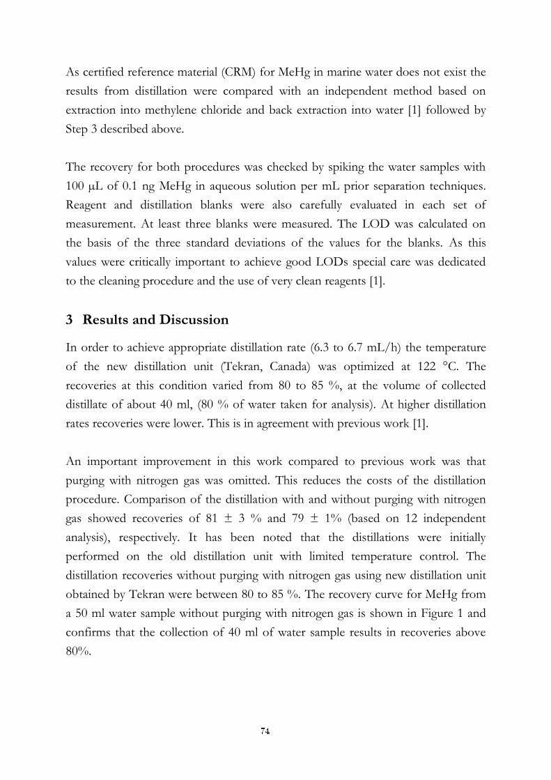
As certified reference material (CRM) for MeHg in marine water does not exist the
results from distillation were compared with an independent method based on
extraction into methylene chloride and back extraction into water [1] followed by
Step 3 described above.
The recovery for both procedures was checked by spiking the water samples with
100 µL of 0.1 ng MeHg in aqueous solution per mL prior separation techniques.
Reagent and distillation blanks were also carefully evaluated in each set of
measurement. At least three blanks were measured. The LOD was calculated on
the basis of the three standard deviations of the values for the blanks. As this
values were critically important to achieve good LODs special care was dedicated
to the cleaning procedure and the use of very clean reagents [1].
3 Results and Discussion
In order to achieve appropriate distillation rate (6.3 to 6.7 mL/h) the temperature
of the new distillation unit (Tekran, Canada) was optimized at 122 °C. The
recoveries at this condition varied from 80 to 85 %, at the volume of collected
distillate of about 40 ml, (80 % of water taken for analysis). At higher distillation
rates recoveries were lower. This is in agreement with previous work [1].
An important improvement in this work compared to previous work was that
purging with nitrogen gas was omitted. This reduces the costs of the distillation
procedure. Comparison of the distillation with and without purging with nitrogen
gas showed recoveries of 81 ± 3 % and 79 ± 1% (based on 12 independent
analysis), respectively. It has been noted that the distillations were initially
performed on the old distillation unit with limited temperature control. The
distillation recoveries without purging with nitrogen gas using new distillation unit
obtained by Tekran were between 80 to 85 %. The recovery curve for MeHg from
a 50 ml water sample without purging with nitrogen gas is shown in Figure 1 and
confirms that the collection of 40 ml of water sample results in recoveries above
80%.
74
Figure 1: Distillation recovery curve for MeHg from 50 ml of sea water
As the pH of the distillate is critically dependent on the reagents added to the
sample prior distillation, the addition of acids was also re-checked. It was found
that the quantity of H2SO4 needs to be lowered as compared to previous protocol
(1 mL of 8 M H2SO4). The optimal recovery (above 80 %) was obtained by the
addition of 0.2 ml 4M H2SO4. In case of the seawater samples that are acidified by
HCl (1% v/v) in the field, it was found that no additional reagents were needed
prior distillation to obtain recoveries above 80%.
Comparison of the results obtained by distillation and extraction is shown in Table
1. Each measurement was done in duplicates. Overall the comparison is good.
However, the precision and sensitivity of the distillation is far better than the
solvent extraction technique. The LOD of the extraction procedure was 1.5 pg/L
and for the distillation 0.42 pg/L.
Table 1: Comparison of the results for MeHg obtained by distillation and solvent extraction
Sample
Extraction [pg/L]
Distillation [pg/L]
Average Average
1 18,8
17,8 13,6
16,7 16,9 19,7
2 41,3
28,5 15,6
15,6 15,6 15,6
3 3,87
7,20 9,40
12,5 10,5 15,7
4 16,1
17,2 21,3
21,0 18,4 20,7
5 58,7
39,5 17,3
16,9 20,3 16,4
6 28,5
23,0 26,8
25,6 17,5 24,5
75

The distillation was also used in real samples from the Mediterranean Sea where expected low concentrations of MeHg were. Results show that concentrations of MeHg in sea water are very low and increase with the depth (1.4 to 72.5 pg/L).
References
[1] M. Horvat, L. Liang, N.S. Bloom. Comparison of distillation with other current isolation methods for the determination of methyl mercury compounds in low level environmental samples: Part II. Water. Analytical Chemical Acta, 282: 153-168, 1993.
[2] J. Kotnik, M. Horvat, E. Tessier, N. Ogrinc, M. Monperrus, D. Amouroux, V. Fajon, D. Gibičar, S. Žižek, F. Sprovieri, N. Pirrone. Mercury speciation in surface and deep waters of the Mediterranean Sea. Marine Chemistry,107: 13-30, 2007
[3] UNEP Chemicals, Global mercury Assessment, Geneva, Switzerland, 2002.
76
For wider interest
The aim of the research is to understand better the chemistry of mercury in
aqueous media. Speciation of chemical species of mercury in water is of ultimate
importance to understand its distribution, partitioning and fate in the environment.
The work presented is focused on the accurate determination of very low
concentrations of a chemical form of mercury – monomethylmercury (MeHg),
which is one of the most toxic compound that accumulates and biomagnifies in
biosphere. Due to very low concentrations found in the environment, especially in
water, the first step was to optimize the procedure and to improve the limit of
detection, so that environmentally consistent data can be obtained. The method
optimized has shown to be fit for purpose as demonstrated on real samples taken
from the Mediterranean Sea. Concentrations in sea water are very low and are
increasing with depth (from 1.4 to 72.5 pg/L). Because of low concentrations it is
necessary to take all the precautions not to contaminate the samples and to use
methods which are the most reliable. That is why the distillation is our method of
choice.
Next steps will include further refinement of the distillation procedure form solid
samples, such as sediments, where the proportion of inorganic mercury can
interfere the analysis by artificial formation of MeHg.
77
Photodegradation of Benzophenones
Kristina Pestotnik1,2, Tina Kosjek1, Uroš Krajnc3, Ester Heath1,2
1 Department of Environmental Sciences, Jožef Stefan Institute, Ljubljana, Slovenia
2 Jožef Stefan International Postgraduate School, Ljubljana, Slovenia
3 Ecological Engineering Institute Ltd, Maribor, Slovenia
Abstract. Over the last decade there has been increasing concern regarding
the presence and possible toxic effects of pharmaceuticals and personal care
products (PPCPs) in the environment. The studied benzophenones include
UV filters, a pharmaceutical, its phototransformation products and others.
The aim of this work was to gain a better understanding of the fate of the
selected benzophenones in the aquatic environment under the influence of
ultraviolet irradiation. Compounds were exposed to UV irradiation using low
pressure (LP) monochromatic mercury lamp with a peak emission at 254 nm
and medium pressure (MP) mercury lamp with a pyrex glass filter. Whereas
ketoprofen was prone to UV irradiation (it was completely degraded after 15
minutes of irradiation with MP lamp), other compounds were found to be
highly resistant. Therefore the efficiency of the UV treatment was increased by
combining UV irradiation (LP lamp) and hydrogen peroxide. As a result of
adding 0.1 % hydrogen peroxide, improved removal of 2-hydroxy-4-
methoxybenzophenone (77 %) and 3-i-propylbenzophenone (92 %) was
achieved.
Keywords: Benzophenones, UV irradiation, photodegradation, UV/H2O2
1 Introduction
An increasing amount of pharmaceuticals and personal care products (PPCPs)
enter the environment globally. In the last decade the problem of the potential
adverse effects on human health and environmental organisms has been found to
be an important aspect of public health. Compounds that include benzophenone
structure (Figure 1) are widely used in various fields. The studied benzophenones
include UV filters (benzophenone, 4-hydroxybenzophenone, 2-hydroxy-4-
78
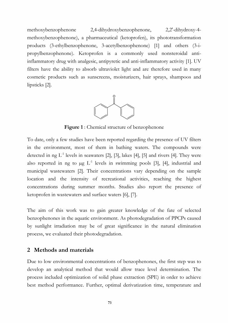
methoxybenzophenone 2,4-dihydroxybenzophenone, 2,2'-dihydroxy-4-
methoxybenzophenone), a pharmaceutical (ketoprofen), its phototransformation
products (3-ethylbenzophenone, 3-acetylbenzophenone) [1] and others (3-i-
propylbenzophenone). Ketoprofen is a commonly used nonsteroidal anti-
inflammatory drug with analgesic, antipyretic and anti-inflammatory activity [1]. UV
filters have the ability to absorb ultraviolet light and are therefore used in many
cosmetic products such as sunscreens, moisturizers, hair sprays, shampoos and
lipsticks [2].
Figure 1 : Chemical structure of benzophenone
To date, only a few studies have been reported regarding the presence of UV filters
in the environment, most of them in bathing waters. The compounds were
detected in ng L-1 levels in seawaters [2], [3], lakes [4], [5] and rivers [4]. They were
also reported in ng to µg L-1 levels in swimming pools [3], [4], industrial and
municipal wastewaters [2]. Their concentrations vary depending on the sample
location and the intensity of recreational activities, reaching the highest
concentrations during summer months. Studies also report the presence of
ketoprofen in wastewaters and surface waters [6], [7].
The aim of this work was to gain greater knowledge of the fate of selected
benzophenones in the aquatic environment. As photodegradation of PPCPs caused
by sunlight irradiation may be of great significance in the natural elimination
process, we evaluated their photodegradation.
2 Methods and materials
Due to low environmental concentrations of benzophenones, the first step was to
develop an analytical method that would allow trace level determination. The
process included optimization of solid phase extraction (SPE) in order to achieve
best method performance. Further, optimal derivatization time, temperature and
79
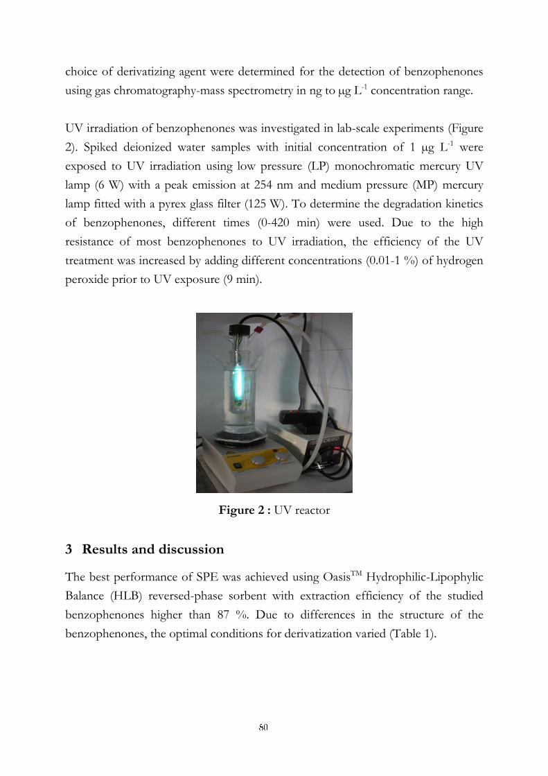
choice of derivatizing agent were determined for the detection of benzophenones
using gas chromatography-mass spectrometry in ng to µg L-1 concentration range.
UV irradiation of benzophenones was investigated in lab-scale experiments (Figure
2). Spiked deionized water samples with initial concentration of 1 µg L-1 were
exposed to UV irradiation using low pressure (LP) monochromatic mercury UV
lamp (6 W) with a peak emission at 254 nm and medium pressure (MP) mercury
lamp fitted with a pyrex glass filter (125 W). To determine the degradation kinetics
of benzophenones, different times (0-420 min) were used. Due to the high
resistance of most benzophenones to UV irradiation, the efficiency of the UV
treatment was increased by adding different concentrations (0.01-1 %) of hydrogen
peroxide prior to UV exposure (9 min).
Figure 2 : UV reactor
3 Results and discussion
The best performance of SPE was achieved using OasisTM Hydrophilic-Lipophylic
Balance (HLB) reversed-phase sorbent with extraction efficiency of the studied
benzophenones higher than 87 %. Due to differences in the structure of the
benzophenones, the optimal conditions for derivatization varied (Table 1).
80
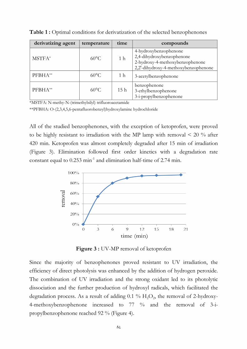
Table 1 : Optimal conditions for derivatization of the selected benzophenones
derivatizing agent temperature time compounds
MSTFA* 60°C 1 h
4-hydroxybenzophenone 2,4-dihydroxybenzophenone 2-hydroxy-4-methoxybenzophenone 2,2'-dihydroxy-4-methoxybenzophenone
PFBHA** 60°C 1 h 3-acetylbenzophenone
PFBHA** 60°C 15 h benzophenone 3-ethylbenzophenone 3-i-propylbenzophenone
*MSTFA: N-methy-N-(trimethylsilyl) trifluoroacetamide
**PFBHA: O-(2,3,4,5,6-pentafluorobenzyl)hydroxylamine hydrochloride
All of the studied benzophenones, with the exception of ketoprofen, were proved
to be highly resistant to irradiation with the MP lamp with removal < 20 % after
420 min. Ketoprofen was almost completely degraded after 15 min of irradiation
(Figure 3). Elimination followed first order kinetics with a degradation rate
constant equal to 0.253 min-1 and elimination half-time of 2.74 min.
Figure 3 : UV-MP removal of ketoprofen
Since the majority of benzophenones proved resistant to UV irradiation, the
efficiency of direct photolysis was enhanced by the addition of hydrogen peroxide.
The combination of UV irradiation and the strong oxidant led to its photolytic
dissociation and the further production of hydroxyl radicals, which facilitated the
degradation process. As a result of adding 0.1 % H2O2, the removal of 2-hydroxy-
4-methoxybenzophenone increased to 77 % and the removal of 3-i-
propylbenzophenone reached 92 % (Figure 4).
81
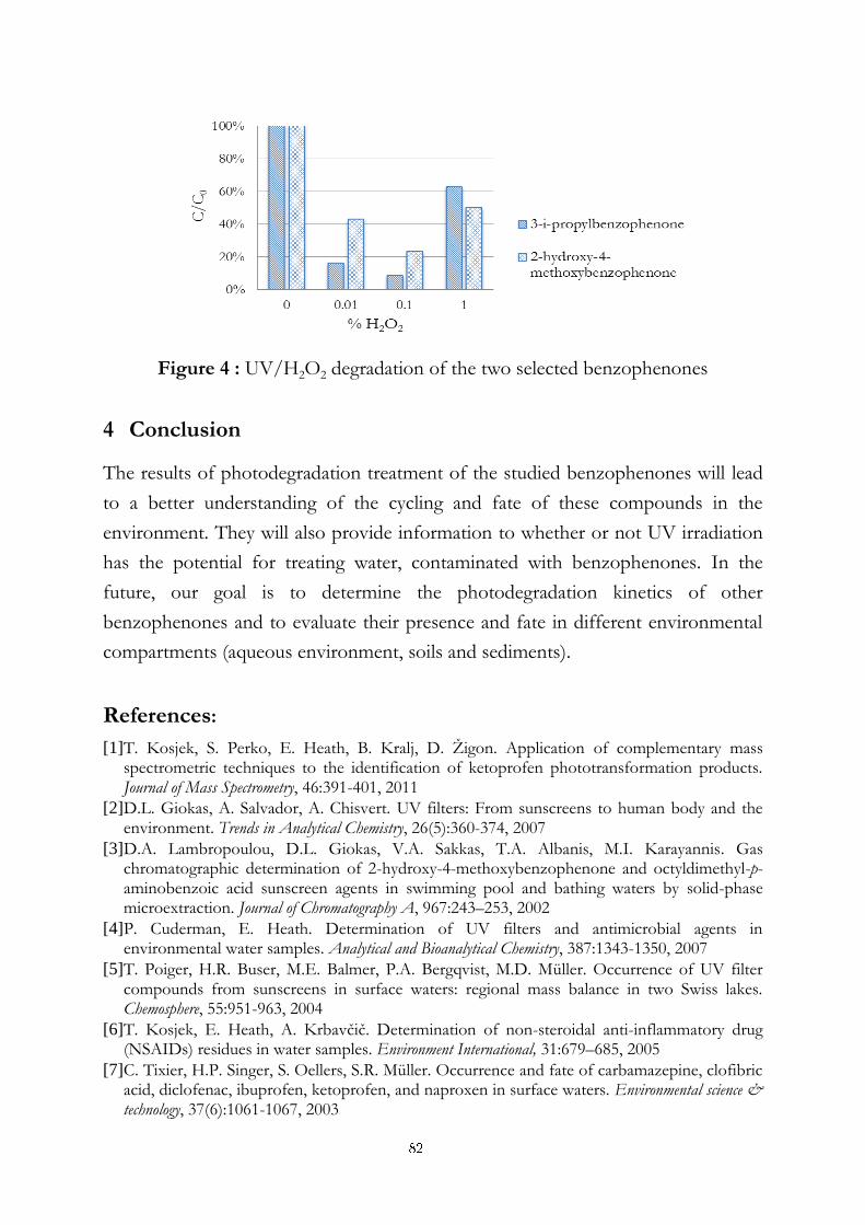
Figure 4 : UV/H2O2 degradation of the two selected benzophenones
4 Conclusion
The results of photodegradation treatment of the studied benzophenones will lead
to a better understanding of the cycling and fate of these compounds in the
environment. They will also provide information to whether or not UV irradiation
has the potential for treating water, contaminated with benzophenones. In the
future, our goal is to determine the photodegradation kinetics of other
benzophenones and to evaluate their presence and fate in different environmental
compartments (aqueous environment, soils and sediments).
References:
[1] T. Kosjek, S. Perko, E. Heath, B. Kralj, D. Žigon. Application of complementary mass spectrometric techniques to the identification of ketoprofen phototransformation products. Journal of Mass Spectrometry, 46:391-401, 2011
[2] D.L. Giokas, A. Salvador, A. Chisvert. UV filters: From sunscreens to human body and the environment. Trends in Analytical Chemistry, 26(5):360-374, 2007
[3] D.A. Lambropoulou, D.L. Giokas, V.A. Sakkas, T.A. Albanis, M.I. Karayannis. Gas chromatographic determination of 2-hydroxy-4-methoxybenzophenone and octyldimethyl-p-aminobenzoic acid sunscreen agents in swimming pool and bathing waters by solid-phase microextraction. Journal of Chromatography A, 967:243–253, 2002
[4] P. Cuderman, E. Heath. Determination of UV filters and antimicrobial agents in environmental water samples. Analytical and Bioanalytical Chemistry, 387:1343-1350, 2007
[5] T. Poiger, H.R. Buser, M.E. Balmer, P.A. Bergqvist, M.D. Müller. Occurrence of UV filter compounds from sunscreens in surface waters: regional mass balance in two Swiss lakes. Chemosphere, 55:951-963, 2004
[6] T. Kosjek, E. Heath, A. Krbavčič. Determination of non-steroidal anti-inflammatory drug (NSAIDs) residues in water samples. Environment International, 31:679–685, 2005
[7] C. Tixier, H.P. Singer, S. Oellers, S.R. Müller. Occurrence and fate of carbamazepine, clofibric acid, diclofenac, ibuprofen, ketoprofen, and naproxen in surface waters. Environmental science & technology, 37(6):1061-1067, 2003
82
For wider interest
The occurrence and fate of pharmaceuticals and personal care products (PPCPs) in
the environment has become one of the emerging issues in environmental
chemistry. This research was conducted to provide a better understanding of the
fate of selected benzophenones in the aquatic environment under the influence of
ultraviolet irradiation. The studied benzophenones include UV filters, a
pharmaceutical (ketoprofen), its phototransformation products and others.
Ketoprofen is a commonly used nonsteroidal anti-inflammatory drug with
analgesic, antipyretic and anti-inflammatory activity. UV filters have the ability to
absorb ultraviolet light and are therefore used in many cosmetic products such as
sunscreen, moisturizer, hair spray, shampoo and lipstick.
As photodegradation of PPCPs caused by sunlight irradiation may be very
important in the natural elimination process, we evaluated the photodegradation of
the selected benzophenones. UV degradation was investigated in lab-scale
experiments using mercury UV lamps. Whereas ketoprofen was prone to UV
irradiation (it was completely degraded after 15 minutes of irradiation), other
compounds were found highly resistant. Therefore the efficiency of the UV
treatment was increased by combining UV irradiation and strong oxidant (hydrogen
peroxide). As a result, the removal of benzophenones increased to up to 92 %.
The results of photodegradation treatment of the studied benzophenones will help
us to get a better understanding of the cycling and fate of these compounds in the
environment. They will also provide information whether UV irradiation has a
potential for treatment of water, contaminated with benzophenones. In the future,
our goal is to evaluate the presence and fate of benzophenones in different
environmental compartments (aqueous environment, soils and sediments).
83
Poly[perfluorotitanate(IV)] Compounds of Alkali Metals, Unexpectedly Complicated Species in the Solid State
Igor Shlyapnikov1,2, Evgeny Goreshnik1, Zoran Mazej1,
1 Department of Inorganic Chemistry and Technology (K1), Jožef Stefan Institute,
Ljubljana, Slovenia
2 Jožef Stefan International Postgraduate School, Ljubljana, Slovenia
Abstract. Experiments carried out between TiF4 and AF (A stands for alkali metals:
Li, Na, K, Rb, Cs) in anhydrous HF (aHF) with different starting molar ratios AF :
TiF4, lead to different compounds. In the case of lithium only one product has been
observed, i.e. Li2TiF6. Reactions between AF (A equals Na, K, Rb) and TiF4 with
starting molar ratios AF : TiF4 = 2 : 1 and 1 : 1 lead to previously known A2TiF6 and
novel ATiF5∙HF salts with infinite polymeric chains ([TiF5]–)n in the crystal
structures. Starting molar ratios AF : TiF4 = 1 : 2 yields novel NaTi2F9∙HF salt with
NaF, meanwhile K4Ti8F36∙8HF and Rb4Ti8F36∙6HF, with previously unknown
octameric anions, have been isolated after reaction with KF and RbF.
Keywords: poly[perfluorotitanate(IV)] compounds, crystal structure,
vibrational spectroscopy
1 Poly[perfluorotitanate(IV)] compounds
A great variety of poly[perfluorotitanate(IV)] compounds with octahedral
coordination of titanium atom can theoretically exist. In all perfluorotitanates Ti4+
ions are in an octahedral coordination of six F atoms, and polymeric ions are
formed by sharing one or two fluorine atoms between two octahedra (shared
apexes or edges – one or two bridging fluorine atoms, respectively). Theoretically,
sharing three fluorine atoms is also possible (two octahedra share face – three
bridging fluorine atoms), but crystal structures of those anions haven’t been
reported yet.
In the solid state polyanions are found as discrete species, chains, double chains,
columns or layers [1,2]. Structures of known poly[perfluorotitanate(IV)] anions are
presented in Figure 1.
84
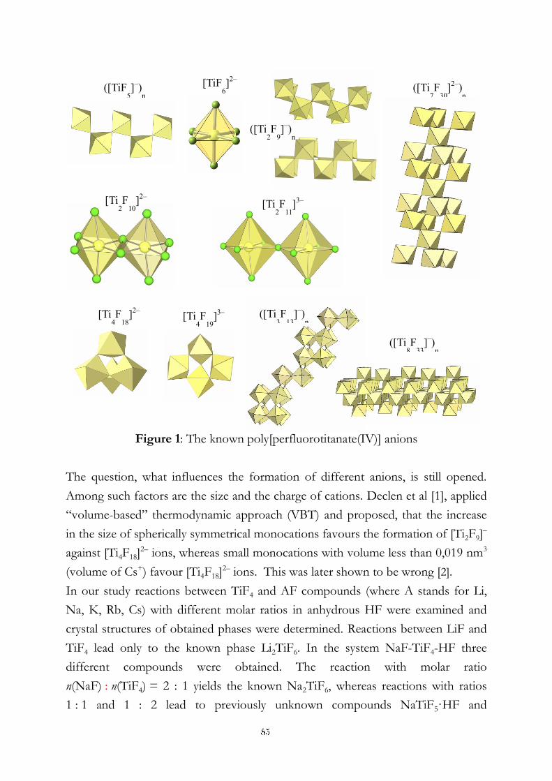
Figure 1: The known poly[perfluorotitanate(IV)] anions
The question, what influences the formation of different anions, is still opened.
Among such factors are the size and the charge of cations. Declen et al [1], applied
“volume-based” thermodynamic approach (VBT) and proposed, that the increase
in the size of spherically symmetrical monocations favours the formation of [Ti2F9]–
against [Ti4F18]2– ions, whereas small monocations with volume less than 0,019 nm3
(volume of Cs+) favour [Ti4F18]2– ions. This was later shown to be wrong [2].
In our study reactions between TiF4 and AF compounds (where A stands for Li,
Na, K, Rb, Cs) with different molar ratios in anhydrous HF were examined and
crystal structures of obtained phases were determined. Reactions between LiF and
TiF4 lead only to the known phase Li2TiF6. In the system NaF-TiF4-HF three
different compounds were obtained. The reaction with molar ratio
n(NaF) : n(TiF4) = 2 : 1 yields the known Na2TiF6, whereas reactions with ratios
1 : 1 and 1 : 2 lead to previously unknown compounds NaTiF5·HF and
([TiF5]–)n [TiF
6]2–
([Ti2F
9]–)n
[Ti2F
10]2–
[Ti2F
11]3–
([Ti7F
30]2–
)n
[Ti4F
18]2–
[Ti4F
19]3– ([Ti
3F
13]–)n
([Ti8F
33]–)n
85
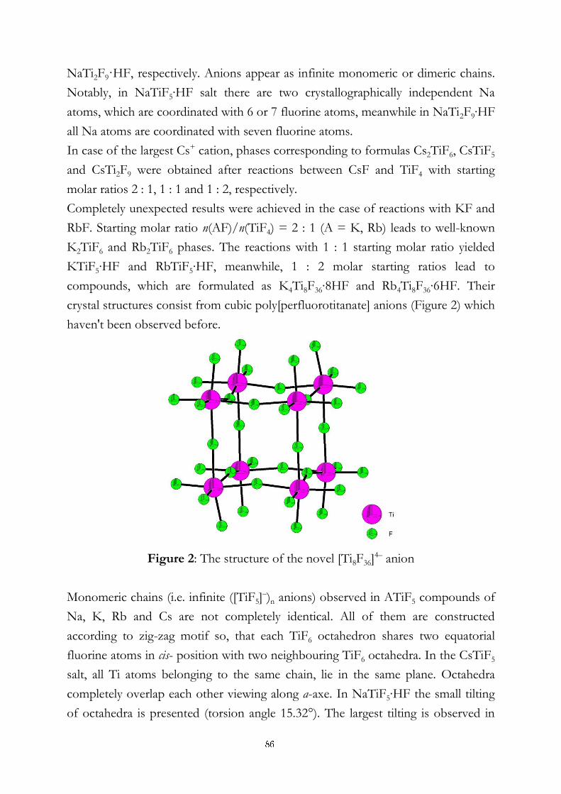
NaTi2F9·HF, respectively. Anions appear as infinite monomeric or dimeric chains.
Notably, in NaTiF5∙HF salt there are two crystallographically independent Na
atoms, which are coordinated with 6 or 7 fluorine atoms, meanwhile in NaTi2F9∙HF
all Na atoms are coordinated with seven fluorine atoms.
In case of the largest Cs+ cation, phases corresponding to formulas Cs2TiF6, CsTiF5
and CsTi2F9 were obtained after reactions between CsF and TiF4 with starting
molar ratios 2 : 1, 1 : 1 and 1 : 2, respectively.
Completely unexpected results were achieved in the case of reactions with KF and
RbF. Starting molar ratio n(AF)/n(TiF4) = 2 : 1 (A = K, Rb) leads to well-known
K2TiF6 and Rb2TiF6 phases. The reactions with 1 : 1 starting molar ratio yielded
KTiF5∙HF and RbTiF5∙HF, meanwhile, 1 : 2 molar starting ratios lead to
compounds, which are formulated as K4Ti8F36∙8HF and Rb4Ti8F36∙6HF. Their
crystal structures consist from cubic poly[perfluorotitanate] anions (Figure 2) which
haven't been observed before.
Figure 2: The structure of the novel [Ti8F36]4– anion
Monomeric chains (i.e. infinite ([TiF5]–)n anions) observed in ATiF5 compounds of
Na, K, Rb and Cs are not completely identical. All of them are constructed
according to zig-zag motif so, that each TiF6 octahedron shares two equatorial
fluorine atoms in cis- position with two neighbouring TiF6 octahedra. In the CsTiF5
salt, all Ti atoms belonging to the same chain, lie in the same plane. Octahedra
completely overlap each other viewing along a-axe. In NaTiF5∙HF the small tilting
of octahedra is presented (torsion angle 15.32°). The largest tilting is observed in
86
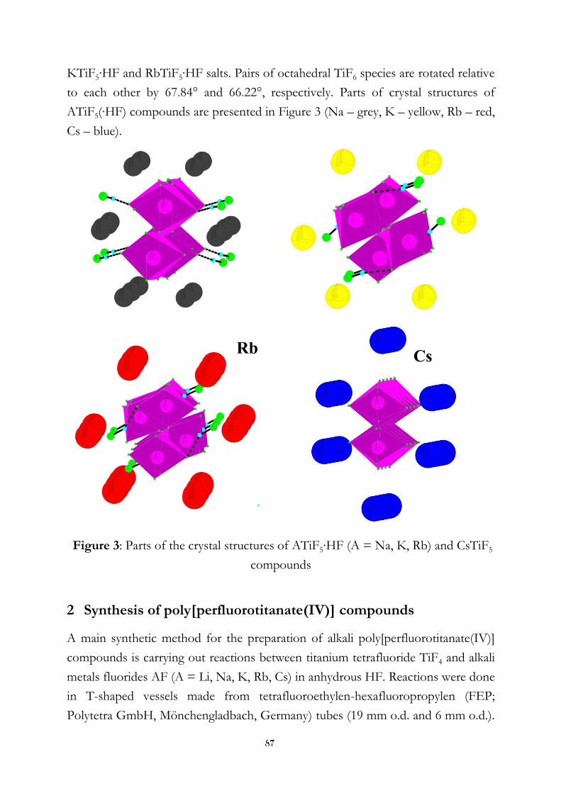
KTiF5∙HF and RbTiF5∙HF salts. Pairs of octahedral TiF6 species are rotated relative
to each other by 67.84° and 66.22°, respectively. Parts of crystal structures of
ATiF5(∙HF) compounds are presented in Figure 3 (Na – grey, K – yellow, Rb – red,
Cs – blue).
Figure 3: Parts of the crystal structures of ATiF5∙HF (A = Na, K, Rb) and CsTiF5
compounds
2 Synthesis of poly[perfluorotitanate(IV)] compounds
A main synthetic method for the preparation of alkali poly[perfluorotitanate(IV)]
compounds is carrying out reactions between titanium tetrafluoride TiF4 and alkali
metals fluorides AF (A = Li, Na, K, Rb, Cs) in anhydrous HF. Reactions were done
in T-shaped vessels made from tetrafluoroethylen-hexafluoropropylen (FEP;
Polytetra GmbH, Mönchengladbach, Germany) tubes (19 mm o.d. and 6 mm o.d.).
Cs Rb
87
The wider tube is sealed from the bottom side and equipped with Teflon T-shaped
cross and Teflon valve from the other side. The narrower tube is connected to the
Teflon T-cross. All manipulations with volatile materials, such as aHF and F2, are
carried out in nickel-Teflon vacuum line and with non-volatile, such as TiF4 – in a
drybox (M. Braun) in an argon atmosphere.
The typical procedure consists from several steps. Firstly, calculated amounts of
reactants (TiF4 and AF, A = Li, Na, K, Rb, Cs) were loaded into the wider arm of a
reaction vessel in the dry box. Argon was pumped away on nickel-Teflon vacuum
line and aHF condensed into the reaction vessel at 77 K. Mixture was warmed to
room temperature and constantly mixed. After one day a solution from the wide
arm of the reactor was decanted into the narrower arm and a temperature gradient
was maintained. When crystals, grown in narrower arm, were still covered with
<1mm of aHF, perfluorinated oil (perfluorodecalin) was injected inside the
narrower tube. The tube was cut and its content transferred to the cooled glass
plate under the microscope. Single crystals were then selected from the
crystallization products under the microscope and then transferred into the cold
nitrogen stream of the diffractometer.
3 Characterisation of poly[perfluorotitanate(IV)] compounds
The synthesised compounds were structurally characterised by means of X-Ray
single crystal structure analysis. Data were collected on a Rigaku AFC7
diffractometer equipped with a Mercury CCD area detector using graphite-
monochromated Mo-Kα radiation (λ = 0,71069 Å) at 200 K. The structures were
solved by direct methods with the use of the SIR-92 program (program package
TeXsan) and refined with the SHELXL-97 software implemented in the program
package WinGX. The figures were prepared using the program DIAMOND 3.1.
References:
[1] A. Decken, H. D. B. Jenkins, C. Knapp, G.B. Nikiforov, J. Passmore, J.M. Rautiainen. The autoionization of [TiF4] by cation complexation with [15]crown-5 to give [TiF2([15]crown-5)][Ti4F18] containing the tetrahedral [Ti4F18]
2– ion. Angew. Chem., Int. Ed., 44:7958-7961, 2005
[2] Z. Mazej, E. Goreshnik. Poly[perfluorotitanate(IV)] salts of [H3O]+, Cs+, [Me4N]+ and [Ph4P]+ and about the existence of an isolated [Ti2F9]
– anion in the solid state. Inorg. Chem., 48:6918-6923, 2009
88
For wider interest
Combining facts, that fluorine is the smallest and the most electronegative
compound in the Periodic Table with the low bond energy in F2 molecule, its
compounds show quite specific properties, which could be very different between
various fluorides (i.e. from great chemical stability to high reactivity, from
resistance to high-temperatures to low temperature decomposition with release of
fluorine). Two typical examples are highly chemically inert polytetrafluoroethylene
(Teflon®) and highly reactive fluorinating agent MnF4. Thus, fluorides could be
successfully applied in various branches of science, technology and everyday life.
Much of the research is usually done due to economic benefits of industrial
processes. But also contributions to fundamental science shouldn’t be missed. They
can’t be precisely evaluated nowadays, but benefit in future. It’s almost impossible
to achieve highest possible results in any branch of human activities without strong
theoretical explanations of processes. And that’s what fundamental science does.
Researches lead to various hypothesis and then to real operating theories and
concepts. Also this work, which is devoted to poly[perfluorotitanate(IV)]
compounds, mostly contributes to fundamental knowledge by collecting
experimental material for understanding mechanisms of synthesis and opens new
ways to selective synthesis of determined perfluorotitanates that then could be used
as selective catalysts in different industrial productions.
89
Vibrational spectra calculation of triphenylene: comparison
of DFT and MP2 methods
Gleb Veryasov1, Dmitry Morozov2, Gašper Tavčar1
1 Department of inorganic chemistry and technology, Jožef Stefan Institute,
Ljubljana, Slovenia
2 Lomonosov Moscow State University, Moscow, Russia
Abstract. The infrared (IR) and Raman spectra of triphenylene with intensities
were calculated using both density functional theory (DFT, B3LYP method)
and Moller-Plesset perturbation method of second order (MP2) with cc-
pVDZ basis set. Spectra were compared with experimentally measured; the
agreement between the observed and calculated spectra is good in case of IR
spectroscopy, MP2 simulated spectra were found have less vibrational band
deviation from the real spectrum. In case of Raman spectroscopy, both
methods gave good band position evaluation, however intensities are hardly
correlated with experimental spectrum.
Keywords: Triphenylene, calculation, vibrational spectra.
1 Introduction
Vibrational spectra of aromatic hydrocarbons were intensively investigated for a
significant period of time [1-7]. Such an investigation is important for developing
trace analyses of these compounds by vibrational spectroscopic techniques, e.g.
surface enchanted spectroscopy [8] and a very useful instrument for band
assignment and detailed investigation of the vibrational spectra.
Detailed triphenylene crystal structure investigation was made by Ahmed and
Trotter [9]. First calculation of vibrational spectra of triphenylene with detailed
band assignments was made by Schettino [10]. Recent works reported were
devoted to density functional theory (DFT) study of vibrational spectra of 1- and 2-
nitrophenylene [8] and theoretical modeling of the influence of structural disorder
on the charge carrier mobility was investigated by Mikolajczyk et. al. [11].
90
Current work provides comparison of applicability of methods – density functional
theory, DFT and Moller-Plesset perturbation theory of the second order, MP2 for
geometry optimization and vibrational spectra calculation of triphenylene by
comparison of calculated spectra and bond distances to experimentally obtained.
2 Experimental part
2.1 Chemicals and instrumentation
Triphenylene was bought from Alfa Aesar.
Raman spectra was measured on triphenylene crystals on Horiba Jobin-Yvon
LabRAM HR High Resolution Raman Spectrometer with internal laser 633 nm and
power of 1,7 mW with total 100 scans.
IR spectrum was measured on PerkinElmer GX spectrometer in KBr cell using
Nujol mull with resolution 1 cm-1.
2.2 Computational details
All calculations were performed using DFT with B3LYP functionals [12-13] and
MP2. All computations were performed carried out using GAMESS(US) program
package [14]. We used cc-pVDZ basis set as well known for correlated methods.
We also used D3h space symmetry group to reduce Hessian evaluation procedure
time. First initial geometry of triphenylene was optimized with both methods, this
gived us minimum energy points from which vibration spectra should be
calculated. Then Forces Constants matrix (also known as Hessian matrix), which is
matrix of the second derivatives of Energy by all coordinates, were calculated.
Normal modes frequencies and corresponding IR intensities were evaluated by
diagonalization of Force Constants matrix. For Raman spectra intensities
polarizability tensor was calculated and then resulting Raman activities (Si) were
converted to Raman intensities (Ii) using following relationship from the intensity
theory of Raman scattering [15-17]:
(1)
Where ν0 – is the exciting frequency (cm-1) and νi – is the vibrational wave number
of the i-th normal mode (cm-1).
91
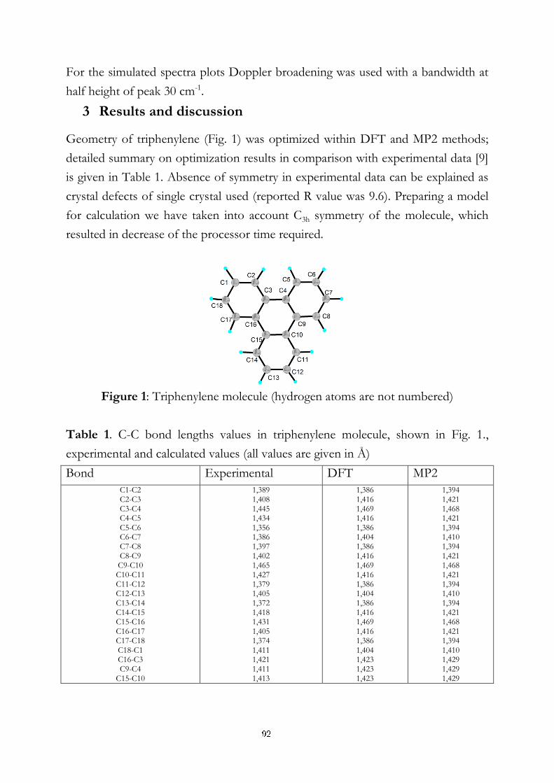
For the simulated spectra plots Doppler broadening was used with a bandwidth at
half height of peak 30 cm-1.
3 Results and discussion
Geometry of triphenylene (Fig. 1) was optimized within DFT and MP2 methods;
detailed summary on optimization results in comparison with experimental data [9]
is given in Table 1. Absence of symmetry in experimental data can be explained as
crystal defects of single crystal used (reported R value was 9.6). Preparing a model
for calculation we have taken into account C3h symmetry of the molecule, which
resulted in decrease of the processor time required.
Figure 1: Triphenylene molecule (hydrogen atoms are not numbered)
Table 1. C-C bond lengths values in triphenylene molecule, shown in Fig. 1.,
experimental and calculated values (all values are given in Å)
Bond Experimental DFT MP2
C1-C2 C2-C3 C3-C4 C4-C5 C5-C6 C6-C7 C7-C8 C8-C9 C9-C10 C10-C11 C11-C12 C12-C13 C13-C14 C14-C15 C15-C16 C16-C17 C17-C18 C18-C1 C16-C3 C9-C4
C15-C10
1,389 1,408 1,445 1,434 1,356 1,386 1,397 1,402 1,465 1,427 1,379 1,405 1,372 1,418 1,431 1,405 1,374 1,411 1,421 1,411 1,413
1,386 1,416 1,469 1,416 1,386 1,404 1,386 1,416 1,469 1,416 1,386 1,404 1,386 1,416 1,469 1,416 1,386 1,404 1,423 1,423 1,423
1,394 1,421 1,468 1,421 1,394 1,410 1,394 1,421 1,468 1,421 1,394 1,410 1,394 1,421 1,468 1,421 1,394 1,410 1,429 1,429 1,429
92
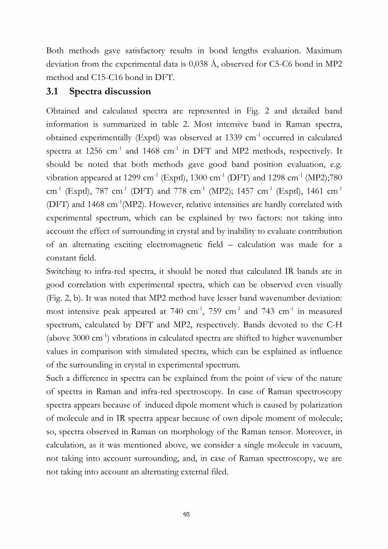
Both methods gave satisfactory results in bond lengths evaluation. Maximum
deviation from the experimental data is 0,038 Å, observed for C5-C6 bond in MP2
method and C15-C16 bond in DFT.
3.1 Spectra discussion
Obtained and calculated spectra are represented in Fig. 2 and detailed band
information is summarized in table 2. Most intensive band in Raman spectra,
obtained experimentally (Exptl) was observed at 1339 cm-1 occurred in calculated
spectra at 1256 cm-1 and 1468 cm-1 in DFT and MP2 methods, respectively. It
should be noted that both methods gave good band position evaluation, e.g.
vibration appeared at 1299 cm-1 (Exptl), 1300 cm-1 (DFT) and 1298 cm-1 (MP2);780
cm-1 (Exptl), 787 cm-1 (DFT) and 778 cm-1 (MP2); 1457 cm-1 (Exptl), 1461 cm-1
(DFT) and 1468 cm-1(MP2). However, relative intensities are hardly correlated with
experimental spectrum, which can be explained by two factors: not taking into
account the effect of surrounding in crystal and by inability to evaluate contribution
of an alternating exciting electromagnetic field – calculation was made for a
constant field.
Switching to infra-red spectra, it should be noted that calculated IR bands are in
good correlation with experimental spectra, which can be observed even visually
(Fig. 2, b). It was noted that MP2 method have lesser band wavenumber deviation:
most intensive peak appeared at 740 cm-1, 759 cm-1 and 743 cm-1 in measured
spectrum, calculated by DFT and MP2, respectively. Bands devoted to the C-H
(above 3000 cm-1) vibrations in calculated spectra are shifted to higher wavenumber
values in comparison with simulated spectra, which can be explained as influence
of the surrounding in crystal in experimental spectrum.
Such a difference in spectra can be explained from the point of view of the nature
of spectra in Raman and infra-red spectroscopy. In case of Raman spectroscopy
spectra appears because of induced dipole moment which is caused by polarization
of molecule and in IR spectra appear because of own dipole moment of molecule;
so, spectra observed in Raman on morphology of the Raman tensor. Moreover, in
calculation, as it was mentioned above, we consider a single molecule in vacuum,
not taking into account surrounding, and, in case of Raman spectroscopy, we are
not taking into account an alternating external filed.
93
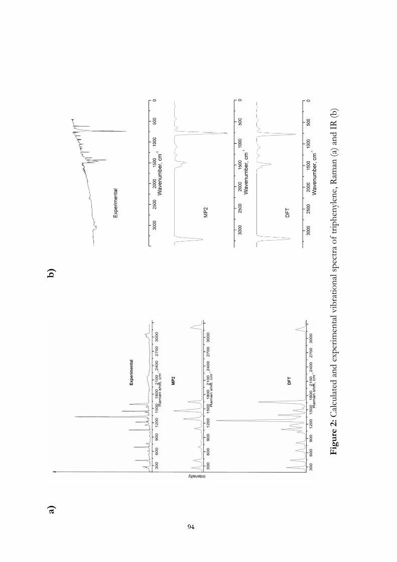
a)
b)
Fig
ure
2:
Cal
cula
ted
an
d e
xp
erim
enta
l vib
rati
on
al s
pec
tra
of
trip
hen
ylen
e, R
aman
(a)
an
d I
R (
b)
94
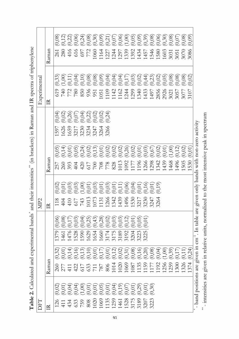
Tab
le 2
. C
alcu
late
d a
nd
exp
erim
enta
l b
ands* a
nd
th
eir
inte
nsi
ties
** (
in b
rack
ets)
in
Ram
an a
nd
IR
sp
ectr
a o
f tr
iph
enyl
ene
DF
T
MP
2
Exp
erim
enta
l
IR
Ram
an
IR
Ram
an
IR
Ram
an
126
(0,0
2)
411
(0,0
1)
434
(0,0
4)
633
(0,0
4)
759
(1,0
0)
808
(0,0
1)
1020 (0
,01)
1069 (0
,05)
1135 (0
,01)
1259 (0
,04)
1461 (0
,19)
1528 (0
,07)
3175 (0
,01)
3189 (0
,29)
3207 (0
,01)
3223 (0
,30)
260
(0,3
2)
1379 (0
,06)
277
(0,0
1)
1461 (0
,08)
411
(0,1
4)
1476 (0
,17)
422
(0,1
6)
1528 (0
,03)
617
(0,1
3)
1590 (0
,04)
633
(0,1
0)
1629 (0
,25)
711
(0,0
1)
1654 (0
,43)
787
(0,1
7)
1660 (0
,28)
806
(0,0
1)
3174 (0
,02)
1014 (0
,12)
3175 (0
,03)
1020 (0
,02)
3189 (0
,03)
1069 (0
,31)
3192 (0
,12)
1087 (0
,08)
3204 (0
,01)
1135 (0
,16)
3223 (0
,05)
1159 (0
,20)
3225 (0
,01)
1177 (0
,08)
1192 (0
,04)
1256 (1
,00)
1259 (0
,39)
1300 (0
,17)
1326 (0
,11)
1374 (0
,24)
118
(0,0
2)
404
(0,0
1)
410
(0,0
3)
617
(0,0
3)
743
(1,0
0)
1013 (0
,01)
1073 (0
,03)
1131 (0
,01)
1266 (0
,03)
1342 (0
,01)
1439 (0
,11)
1496 (0
,06)
1530 (0
,04)
3217 (0
,01)
3230 (0
,16)
3247 (0
,01)
3264 (0
,19)
257
(0,0
5)
1597 (0
,04)
260
(0,1
4)
1626 (0
,02)
393
(0,0
1)
1659 (0
,26)
404
(0,0
5)
3217 (0
,07)
420
(0,2
4)
3230 (0
,04)
617
(0,0
2)
3234 (0
,22)
700
(0,1
3)
3247 (0
,02)
708
(0,0
1)
3264 (0
,02)
778
(0,0
2)
3266 (0
,24)
828
(0,0
2)
1013 (0
,02)
1092 (0
,26)
1177 (0
,02)
1196 (0
,01)
1266 (0
,03)
1298 (0
,67)
1342 (0
,02)
1439 (0
,01)
1468 (1
,00)
1496 (0
,12)
1505 (0
,02)
1530 (0
,01)
619 (0
,33)
740 (1
,00)
772 (0
,11)
780 (0
,04)
850 (0
,10)
936 (0
,08)
951 (0
,08)
1051 (0
,09)
1109 (0
,04)
1142 (0
,04)
1162 (0
,04)
1244 (0
,17)
1299 (0
,03)
1340 (0
,02)
1433 (0
,44)
1497 (0
,23)
2856 (0
,02)
2926 (0
,05)
3021 (0
,08)
3057 (0
,08)
3077 (0
,08)
3107 (0
,02)
261 (0
,08)
280 (0
,12)
416 (0
,22)
616 (0
,06)
697 (0
,24)
772 (0
,08)
1060 (0
,30)
1164 (0
,09)
1227 (0
,21)
1244 (0
,07)
1297 (0
,06)
1339 (1
,00)
1392 (0
,05)
1434 (0
,09)
1457 (0
,39)
1546 (0
,08)
1580 (0
,06)
1603 (0
,30)
3031 (0
,08)
3051 (0
,07)
3070 (0
,08)
3086 (0
,09)
* -
ban
d p
osi
tio
ns
are
given
in
cm
-1. In
tab
le a
re g
iven
on
ly b
and
s w
ith
no
n-z
ero
act
ivit
y **
- in
ten
siti
es a
re g
iven
in
rel
ativ
e un
its,
no
rmal
ized
to
th
e m
ost
in
ten
sive
pea
k in
sp
ectr
um
95
3 Conclusions
Geometry optimization and vibrational spectra calculation within density functional
method, DFT and Moller-Plesset perturbation of second order, MP2 were made in
GAMESS(US) program package. Comparison of data obtained with experimentally
measured spectra and bond distances, available in literature showed that both
method give good evaluation of the atom bond distances and normal frequencies
for the IR spectra, except C-H vibrations region, which appear at lower
wavenumber values in experimentally obtained spectrum, what can be explained as
influence of the surrounding in solid phase. For Raman spectroscopy both
methods gave good evaluation of band positions, however intensities are hardly
correlated to the real spectrum because of absence of opportunity to take into
account effect of the surrounding and of an alternating exciting electromagnetic
field. It shows that IR spectra calculation for the moment is more promising for
qualitative correlation of calculated and experimental spectra.
To summarize, both methods are suitable for spectra calculation; MP2 method
showed lesser band position deviation from the both experimentally obtained
spectra – Raman and IR.
References:
[1] V. Schettino, N. Neto, and S. Califano, J. Chem. Phys. 44, 2724, 1966
[2] V. Schettino, J. Chem. Phys. 46, 302, 1967
[3] R. Mecke and K. Witt, Z. Naturforsch. A 21, 1899, 1966
[4] R. Mecke and K. Witt, Z. Naturforsch. A 21, 1247, 1967
[5] J. Semmler, P. W. Yang, G. E. Crawford, Vibr. Spectrosc. 2, 189, 1991
[6] K. Meerkel, A. Kocot, R. Wrzalik, B. Orgasinsak, Acta. Phys. Pol. A 98, 525, 2000
[7] D. M. Hugins, S. A. Sandford, J. Phys. Chem. A 102, 329, 1198
[8] K. K. Onchoke, M. E. Parks, A. H. Nolan, Spectrochim. Acta A 74, 579, 2009
[9] F. R. Ahmed and J. Trotter, Acta. Cryst. 16, 503, 1963
[10]V. Schettino, J. Mol. Spectrosc.24, 78, 1970
[11]M. M Mikolajczyk, P. Toman, W. Bartkowiak, Chem. Phys. Lett. 485, 253, 2010
[12]A. D. Becke, J. Chem. Phys.98, 5648, 1993
[13]C. Lee, W. Yang, R. G. Parr, Phys. Rew. B 37, 785, 1998
[14] M. W. Schmidt, K. K. Baldridge, J. A. Boatz, S. T. Elbert, M. S. Gordon, J. J. Jensen, S. Koseki, N. Matsunaga, K. A. Nguyen, S. Su, T. L. Windus, M. Dupuis, J. A. Montgomery, J. Comput. Chem. 14, 1347, 1993
[15] P. L. Polavarapu, J. Phys. Chem. 94, 8106, 1990 (RAMAN)
[16]G. Keresztury, Raman spectroscopy: theory, in: J. M. Chalmers, P. R. Griffiths (Eds.), Handbook of Vibrational Spectroscopy, vol. 1., Wiley, 2002, 71-87
[17]G. Keresztury, S. Holly, J. Varga, G. Besenyei, A. Y. Wang, J. R. Durig, Spectrochim. Acta 49 A, 2007, 1993
96

For wider interest
Computational methods in chemistry, or just “calculations” is a powerful
instrument for revealing mechanisms of reactions, theoretical modeling of different
processes and molecules. Modern supercomputers allow to model and even predict
reactions even in such complicated tasks in biological systems as fermentative
reactions, where geometry of an active center in molecule play fundamental role.
This research is devoted to spectroscopy of aromatic hydrocarbons; we focused on
two vibrational spectroscopy methods – Raman spectroscopy and infra-red
spectroscopy (IR). Current work provides investigation of applicability of two
calculation methods – density functional theory (DFT) and Moller-Plesset
perturbation theory of second order (MP2). Applicability of methods was evaluated
by comparison of calculated atomic coordinates and spectra with in literature
available coordinates and experimentally obtained spectra. This investigation
contributes to the building of the model for further calculations of more
complicated structures, containing polycyclic aromatic hydrocarbons (PAH), e.g.
complex compounds, which can include PAH molecules as a π- donor ligands or
different PAH nitro- derivatives, which were proved to be mutagenic . Opportunity
to predict and calculate spectra can help in understanding and detailed investigation
of spectra of these compounds and, moreover, help to invent more precise
methods for trace analysis of pollutants by sensitive spectroscopic methods.
97
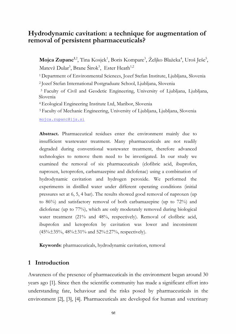
Hydrodynamic cavitation: a technique for augmentation of removal of persistent pharmaceuticals?
Mojca Zupanc1,2, Tina Kosjek1, Boris Kompare3, Željko Blažeka4, Uroš Ješe5,
Matevž Dular5, Brane Širok5, Ester Heath1,2
1 Department of Environmental Sciences, Jozef Stefan Institute, Ljubljana, Slovenia
2 Jozef Stefan International Postgraduate School, Ljubljana, Slovenia
3 Faculty of Civil and Geodetic Engineering, University of Ljubljana, Ljubljana, Slovenia
4 Ecological Engineering Institute Ltd, Maribor, Slovenia 5 Faculty of Mechanic Engineering, University of Ljubljana, Ljubljana, Slovenia
Abstract. Pharmaceutical residues enter the environment mainly due to
insufficient wastewater treatment. Many pharmaceuticals are not readily
degraded during conventional wastewater treatment, therefore advanced
technologies to remove them need to be investigated. In our study we
examined the removal of six pharmaceuticals (clofibric acid, ibuprofen,
naproxen, ketoprofen, carbamazepine and diclofenac) using a combination of
hydrodynamic cavitation and hydrogen peroxide. We performed the
experiments in distilled water under different operating conditions (initial
pressures set at 6, 5, 4 bar). The results showed good removal of naproxen (up
to 86%) and satisfactory removal of both carbamazepine (up to 72%) and
diclofenac (up to 77%), which are only moderately removed during biological
water treatment (21% and 48%, respectively). Removal of clofibric acid,
ibuprofen and ketoprofen by cavitation was lower and inconsistent
(45%±35%, 48%±31% and 52%±27%, respectively).
Keywords: pharmaceuticals, hydrodynamic cavitation, removal
1 Introduction
Awareness of the presence of pharmaceuticals in the environment began around 30
years ago [1]. Since then the scientific community has made a significant effort into
understanding fate, behaviour and the risks posed by pharmaceuticals in the
environment [2], [3], [4]. Pharmaceuticals are developed for human and veterinary
98
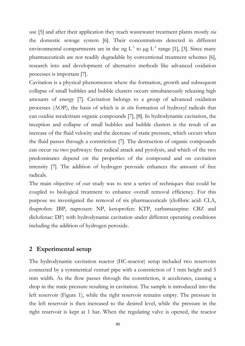
use [5] and after their application they reach wastewater treatment plants mostly via
the domestic sewage system [6]. Their concentrations detected in different
environmental compartments are in the ng L-1 to µg L-1 range [1], [3]. Since many
pharmaceuticals are not readily degradable by conventional treatment schemes [6],
research into and development of alternative methods like advanced oxidation
processes is important [7].
Cavitation is a physical phenomenon where the formation, growth and subsequent
collapse of small bubbles and bubble clusters occurs simultaneously releasing high
amounts of energy [7]. Cavitation belongs to a group of advanced oxidation
processes (AOP), the basis of which is in situ formation of hydroxyl radicals that
can oxidise recalcitrant organic compounds [7], [8]. In hydrodynamic cavitation, the
inception and collapse of small bubbles and bubble clusters is the result of an
increase of the fluid velocity and the decrease of static pressure, which occurs when
the fluid passes through a constriction [7]. The destruction of organic compounds
can occur via two pathways: free radical attack and pyrolysis, and which of the two
predominates depend on the properties of the compound and on cavitation
intensity [7]. The addition of hydrogen peroxide enhances the amount of free
radicals.
The main objective of our study was to test a series of techniques that could be
coupled to biological treatment to enhance overall removal efficiency. For this
purpose we investigated the removal of six pharmaceuticals (clofibric acid: CLA,
ibuprofen: IBP, naproxen: NP, ketoprofen: KTP, carbamazepine: CBZ and
diclofenac: DF) with hydrodynamic cavitation under different operating conditions
including the addition of hydrogen peroxide.
2 Experimental setup
The hydrodynamic cavitation reactor (HC-reactor) setup included two reservoirs
connected by a symmetrical venturi pipe with a constriction of 1 mm height and 5
mm width. As the flow passes through the constriction, it accelerates, causing a
drop in the static pressure resulting in cavitation. The sample is introduced into the
left reservoir (Figure 1), while the right reservoir remains empty. The pressure in
the left reservoir is then increased to the desired level, while the pressure in the
right reservoir is kept at 1 bar. When the regulating valve is opened, the reactor
99
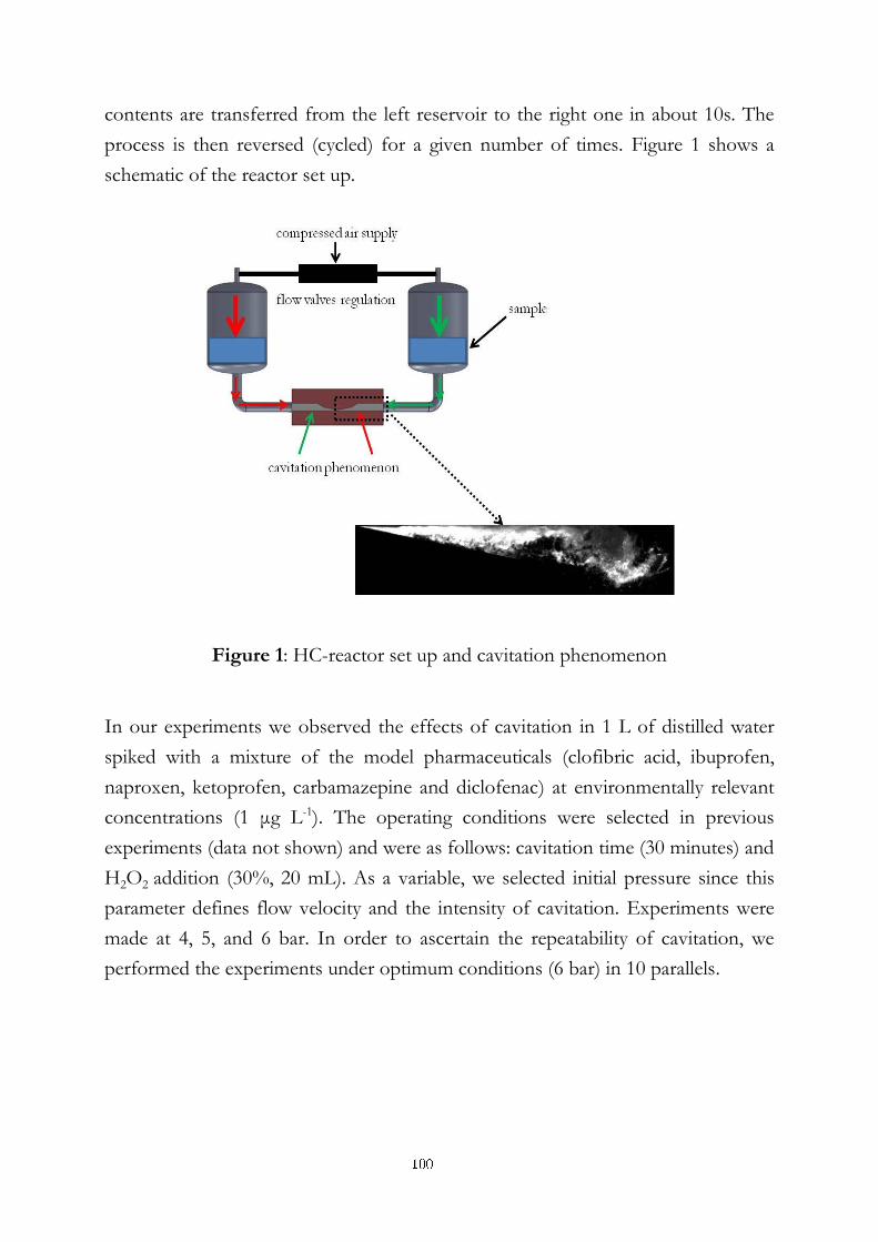
contents are transferred from the left reservoir to the right one in about 10s. The
process is then reversed (cycled) for a given number of times. Figure 1 shows a
schematic of the reactor set up.
Figure 1: HC-reactor set up and cavitation phenomenon
In our experiments we observed the effects of cavitation in 1 L of distilled water
spiked with a mixture of the model pharmaceuticals (clofibric acid, ibuprofen,
naproxen, ketoprofen, carbamazepine and diclofenac) at environmentally relevant
concentrations (1 μg L-1). The operating conditions were selected in previous
experiments (data not shown) and were as follows: cavitation time (30 minutes) and
H2O2 addition (30%, 20 mL). As a variable, we selected initial pressure since this
parameter defines flow velocity and the intensity of cavitation. Experiments were
made at 4, 5, and 6 bar. In order to ascertain the repeatability of cavitation, we
performed the experiments under optimum conditions (6 bar) in 10 parallels.
100
3 Results and discussion
The results show that highest removal of all six pharmaceuticals was achieved at 6
bar (Figure 2). This was in agreement with the presumption that a higher initial
pressure results in an increase in cavitation intensity. The removal of
pharmaceuticals at 5 bar was slightly better than at 4 bar.
Figure 2: Removals (%) of pharmaceuticals with hydrodynamic cavitation under
different initial pressures (6, 5 and 4 bars)
At 6 bar we achieved 86%±8% removal of naproxen and 72%±14% and
77%±12% of carbamazepine and diclofenac, respectively. The removal efficiencies
of clofibric acid, ibuprofen and ketoprofen were lower and inconsistent compared
to naproxen. As mentioned before the destruction of organic compounds with
hydrodynamic cavitation is dependent on their structure and chemical properties
and the different chemical structure of the selected pharmaceuticals may be the
reason for different removal efficiencies.
Since carbamazepine and diclofenac are not readily and consistently removed
during biological waste water treatment (21% and 48%, respectively), which we
established in our previous work and is in accordance with the literature [8], [9],
hydrodynamic cavitation could be a viable technique for augmenting their removal.
To authors knowledge few data exist regarding the removal of pharmaceuticals
using hydrodynamic cavitation. Since cavitation is a technique that is relatively easy
to scale up [10], it should be given more attention.
101
In the future we will combine hydrodynamic cavitation and Fenton process to
achieve better removal of recalcitrant pharmaceuticals (clofibric acid, ibuprofen and
ketoprofen) and further augment the removal of naproxen, carbamazepine and
diclofenac. After the determination of removal efficiencies and optimal operational
conditions for this combination in distilled water, we will transfer the technology to
more complex matrices (effluents of biological wastewater treatment plants). Last
but not least, our aim is to determine the best combination of different processes
considering removal of pharmaceuticals, feasibility and cost effectiveness, possibly
coupling AOP sequentially to biological treatment.
References:
[1] J. P. Bound, K. Kitsou, N. Voulvoulis. Household disposal of pharmaceuticals and perception of risk to the environment. Environmental Toxicology and Pharmacology, 21: 301–307, 2006
[2] Halling-Sørensen B., Nors Nielsen S., Lanzky P.F:, Ingerslev F., Holten Lützhøft, Jørgensen. Occurence, Fate and Effects of Pharmaceutical Substances in the Environment – A Review. Chemosphere, 36 : 357-393, 1998
[3] Ternes T.A., Giger W., Joss A. Introduction. In: Human Pharmaceuticals, Hormones and Fragrances: The challenge of micropollutants in urban water management. Ternes T.A., Joss A., 2006.
[4] Farre M., Perez S., Kantiani L., Barcelo D. Fate and toxicity of emerging pollutants, their metabolites and transformation products in the aquatic environment. Trends in Analytical Chemistry, 27 : 991-1007, 2008
[5] O.V. Enick, M.M. Moore. Assessing the assessments: Pharmaceuticals in the environment. Environmental Impact Assessment Review , 27: 707–729, 2007
[6] A. Joss, S. Zabczynski, A. Göbel, B. Hoffmann, D. Löffler, C. S. McArdell, T. A. Ternes, A. Thomsea, H. Siegrist. Biological degradation of pharmaceuticals in municipal wastewater treatment: Proposing a classification scheme. Water Research, 40: 1686 – 1696, 2006
[7] P.R. Gogate, A.B. Pandit. A review of imperative technologies for wastewater treatment I:oxidation technologies at ambient conditions. Advances in Environmental Research, 8: 501-551, 2004
[8] P. Braeutigam , M. Franke, R. J. Schneider , A. Lehmann , A. Stolle, B. Ondruschka. Degradation of carbamazepine in environmentally relevant concentrations in water by Hydrodynamic-Acoustic-Cavitation (HAC). Water Research, 46: 2469-2477, 2012
[9] M. Ravina, L. Campanella, J. Kiwi. Accelerated mineralization of the drug Diclofenac via Fenton reactions in a concentric photo-reactor. Water research, 36: 3553-3560, 2002
[10] A.G. Chakinala, P.R. Gogate, A.E. Burgess, D.H. Bremner. Treatment of industrial wastewater effluents using hydrodynamic cavitation and the advanced Fenton process. Ultrasonics Sonochemistry, 15: 49-54, 2008
102
For wider interest
To meet the ever growing demand for improved healthcare, pharmaceuticals are
being produced in increasing amounts. As a consequence, pharmaceutical residues
in the environment are becoming a concern. This is because many of these
compounds have been proven to be resistant to conventional microbiological
wastewater treatment. In response, new technologies are necessary to reach
increasingly stringent regulation on water quality.
In this study we investigated hydrodynamic cavitation which is a potent advanced
oxidation process (AOP) and is relatively cost-effective and easy for scale up.
Caviation is the term given to the formation and subsequent implosion of bubbles
that result when the partial local pressure in a fluid drops below vapour pressure.
The collapse of the bubbles can generate a significant increase in local pressures
and temperatures, called “hot spots”. Such extreme conditions can result in the
formation of free radicals, which are potent oxidising species capable of breaking
down organic compounds. Our intention is to make use of these free radicals by
deliberately cavitating the effluent flow from a wastewater plant. Additionally, our
idea is to increase the amount of free radicals formed by adding hydrogen peroxide.
Initial experiments have been carried out using a two reservoir system in which the
fluid can be transferred from one to the other by varying the pressures in each. As
the fluid passes from one reservoir to the other, it must pass through a
constriction, which creates a pressure drop in the fluid resulting in cavitation. We
tested the apparatus using six common pharmaceuticals: clofibric acid, ibuprofen,
naproxen, ketoprofen, carbamazepine and diclofenac at various pressures 4, 5 and 6
bar. A pressure of six bars was optimum. In the case of carbamazepine and
diclofenac, the results have been positive, improving the removal efficiency by 50%
and 30 %, respectively, compared to conventional water treatment. In the case of
clofibric acid, ibuprofen and ketoprofen the results are less conclusive. Further
study will involve optimisation of cavitation process and its combination with
biological water treatment in order to improve overall removal of resistant
contaminants.
103


Informacijske in komunikacijske tehnologije
(Information and Communication Technologies)
105

Reducing costs with computer power management
Lucas Benedičič1, Peter Korošec
2
1 Jožef Stefan International Postgraduate School, Ljubljana, Slovenia
2 Computer Systems Department, Jožef Stefan Institute, Ljubljana, Slovenia
Abstract. In this work, we present a software-based solution to automate the
power control of desktop computers. The deployment of the proposed
software system is simply done over the existing infrastructure of the
organization, thus minimizing the required investment. Our initial analysis
shows a cost reduction of more than 52% by reducing the power
consumption of computers and their monitors.
Keywords: energy, efficiency, automatic control, computer.
1 Introduction
Information technology (IT) has an enormous potential for implementing
environmentally-friendly practices. As Sheehan explains in [1], IT is a major
consumer of energy and a net contributor of greenhouse gas emissions and other
forms of waste. In a report by Gartner Inc., cited in [1], it is estimated that the IT
industry is responsible for 2% of global CO2 emissions. This a priori relatively small
percentage is actually equivalent to the impact the airline industry has in the
environment [2].
Different works have been published confirming the ineffective use of energy in IT
[3], [4], but only some of them implement solutions to tackle this problem [5].
Unfortunately, most of these systems impose significant obstacles to practical
deployment, by either requiring modifications to network interface hardware or, in
some cases, the host operating system software.
We propose a software-based solution to save power by automatically turning
personal computers (PCs) off (without user's intervention) when they are not being
107
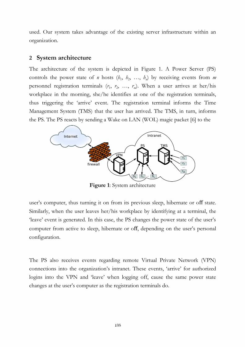
used. Our system takes advantage of the existing server infrastructure within an
organization.
2 System architecture
The architecture of the system is depicted in Figure 1. A Power Server (PS)
controls the power state of n hosts (h1, h2, …, hn) by receiving events from m
personnel registration terminals (r1, r2, …, rm). When a user arrives at her/his
workplace in the morning, she/he identifies at one of the registration terminals,
thus triggering the ‘arrive’ event. The registration terminal informs the Time
Management System (TMS) that the user has arrived. The TMS, in turn, informs
the PS. The PS reacts by sending a Wake on LAN (WOL) magic packet [6] to the
Figure 1: System architecture
user’s computer, thus turning it on from its previous sleep, hibernate or off state.
Similarly, when the user leaves her/his workplace by identifying at a terminal, the
‘leave’ event is generated. In this case, the PS changes the power state of the user’s
computer from active to sleep, hibernate or off, depending on the user’s personal
configuration.
The PS also receives events regarding remote Virtual Private Network (VPN)
connections into the organization’s intranet. These events, ‘arrive’ for authorized
logins into the VPN and ‘leave’ when logging off, cause the same power state
changes at the user’s computer as the registration terminals do.
108
3 Implementation
3.1 Server side
The PS is entirely implemented as a web application. Hypertext transfer protocol
secure (HTTPS) is used to transfer common HTML pages, which are used for the
administration tasks and adjusting the users’ configuration. Each of the ‘arrive’ and
‘leave’ events are accessed through their own uniform resource identifier (URI)
over HTTPS, enforcing additional authentication to avoid misuse and emphasize
the security aspect, e.g. https://ps.example.si/usr_id/wakeup, where usr_id is a key
that uniquely identifies the user that generated the event, either by arriving at
her/his workplace or by connecting to the organization’s VPN. On the other hand,
https://ps.example.si/usr_id/sleep, handles the event triggered by the user leaving
office or disconnecting from the VPN.
3.2 Host side
A Service Application (SA) runs on every host (h1, h2, …, hn as marked in Figure 1)
that is controlled by the PS. The main objective of the SA is to make sure that the
centrally-controlled power schema, imposed by the PS, does not conflict with the
user’s activities. Such situations appear, for example, when the user starts a long-
running process that finishes after the user has left, or when dealing with software
updates, or even with long file transfers like backup operations. The SA makes sure
that the host changes its power state only after the on-going execution has finished.
To achieve this, it is constantly monitoring processor usage and network activity on
the host after the ‘sleep’ message has been received from the PS. Once both
monitored measures fall below the configured threshold for a given amount of
time, the previously queued power-state change is executed.
4 Analysis
Power consumption measurements were taken using a Voltcraft Energy Check
3000 power meter. A total of 30 computers were measured, including different
hardware, software and operating systems. The power consumption of each
computer was continuously measured for 24 hours, separating between active (the
109
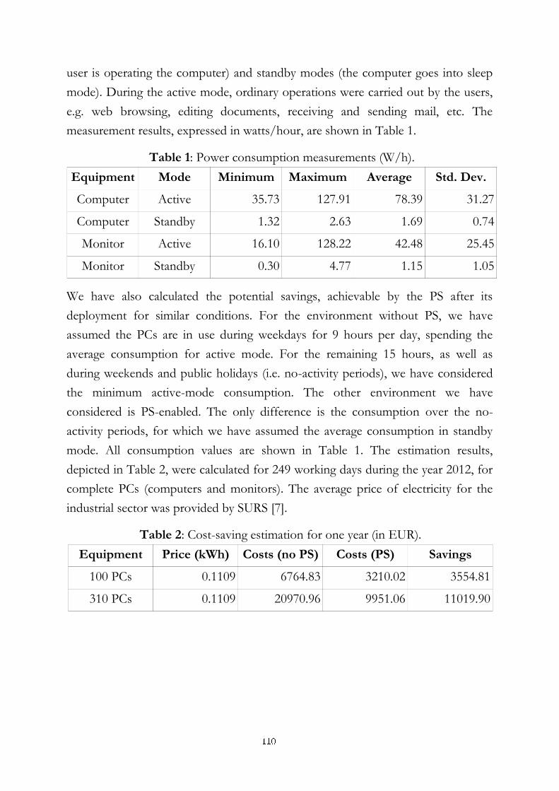
user is operating the computer) and standby modes (the computer goes into sleep
mode). During the active mode, ordinary operations were carried out by the users,
e.g. web browsing, editing documents, receiving and sending mail, etc. The
measurement results, expressed in watts/hour, are shown in Table 1.
We have also calculated the potential savings, achievable by the PS after its
deployment for similar conditions. For the environment without PS, we have
assumed the PCs are in use during weekdays for 9 hours per day, spending the
average consumption for active mode. For the remaining 15 hours, as well as
during weekends and public holidays (i.e. no-activity periods), we have considered
the minimum active-mode consumption. The other environment we have
considered is PS-enabled. The only difference is the consumption over the no-
activity periods, for which we have assumed the average consumption in standby
mode. All consumption values are shown in Table 1. The estimation results,
depicted in Table 2, were calculated for 249 working days during the year 2012, for
complete PCs (computers and monitors). The average price of electricity for the
industrial sector was provided by SURS [7].
Table 1: Power consumption measurements (W/h).
Equipment Mode Minimum Maximum Average Std. Dev.
Computer Active 35.73 127.91 78.39 31.27
Computer Standby 1.32 2.63 1.69 0.74
Monitor Active 16.10 128.22 42.48 25.45
Monitor Standby 0.30 4.77 1.15 1.05
Table 2: Cost-saving estimation for one year (in EUR).
Equipment Price (kWh) Costs (no PS) Costs (PS) Savings
100 PCs 0.1109 6764.83 3210.02 3554.81
310 PCs 0.1109 20970.96 9951.06 11019.90
110
5 Conclusion
We have presented an innovative solution for computer power management that
automatically turns PCs off when they are not in use. The solution installation
requires a minimal initial investment, since it is completely software-based and
takes advantage of the existing infrastructure. The initial results of our analysis
show a cost reduction of more than 52%, saving more than 10,000 EUR a year
from of a group of 300 PCs.
References
[1] M.C. Sheehan, S.D. Smith, and EDUCAUSE Centre for Applied Research. Powering Down: Green IT in Higher Education. EDUCAUSE, 2010.
[2] C. Pettey. Gartner estimates ICT industry accounts for 2 percent of global CO2 emissions. http://www.gartner.com/it/page.jsp, 2007.
[3] M. Chetty, AJ Brush, B.R. Meyers, and P. Johns. It’s not easy being green: understanding home computer power management. In Proceedings of the 27th international conference on Human factors in computing systems, pages 1033–1042. ACM, 2009.
[4] E. Reinhard, B. Champion, N.N. Schulz, R. Gould, E. Perez, and N. Brown. Computer power consumption and management: earth, wind, and fire: Sustainable energy for the 21st century. In Power Systems Conference and Exposition (PSCE), 2011 IEEE/PES, pages 1–8. IEEE, 2011.
[5] Y. Agarwal, S. Hodges, R. Chandra, J. Scott, P. Bahl, and R. Gupta. Somniloquy: augmenting network interfaces to reduce PC energy usage. In Proceedings of the 6th USENIX symposium on Networked systems design and implementation, pages 365–380. USENIX Association, 2009.
[6] S.T. Bui. Wake on LAN power management, 2006, US Patent. 11/403, 452. [7] M. Suvorov and J. Zalar. Statistični urad RS - Cene energentov, Slovenija, 1. polletje 2011,
http://www.stat.si/novica_prikazi.aspx?id=4151, 2012.
111
For wider interest
Many organizations are increasingly leaving their networked computers turned on
24 hours a day, 7 days a week, to allow for out-of-hours access by employees. Some
administrators may say they want to do a backup, or the user may want to be able
to remotely connect into her/his computer. But most of the time these personal
computers (PCs) remain idle, wasting significant amounts of energy.
In this work, we present a software-based solution to automate the power control
of desktop PCs. The deployment of the proposed system is simply done over the
existing infrastructure (i.e. hardware) of the organization, thus minimizing the
required investment. The controlling software, named Power Server, reads events
from the personnel registration terminals. These events generate the power-state
changes of the owner's PC, turning it on when arriving to office, and off when
leaving home. Power Server also reacts to remote VPN connections in a similar
way. The user may also modify the configuration and select, for example, to put the
PC into a low-energy sleep or hibernation mode instead of turning it off.
The energy savings come from the fact that each PC is kept running strictly for the
time it is being used, neither more nor less. Since even the latest low-power
desktop PCs consume around 40 watts of power when idle, the potential savings of
a Power Server installation are very promising: more than 52% of energy-
consumption reduction, which means more than 10,000 EUR a year for an
organization hosting just 300 desktop PCs.
There is other software that can be used to wake up sleeping PCs, such as Apple's
Wake-on Demand and Microsoft's Sleep Proxy, but none of them provides the
needed level of flexibility to maximize energy savings. Moreover, Power Server
works without user's intervention, since the power-state changes are automatically
performed, based on external events.
112
Risk Assessment Using Local Outlier Factor Algorithm
Božidara Cvetković1,2, Mitja Luštrek1,2
1 Department of Intelligent Systems, Jožef Stefan Institute, Ljubljana, Slovenia
2 Jožef Stefan International Postgraduate School, Ljubljana, Slovenia
Abstract. In this paper we introduce the unsupervised machine-learning
algorithm named Local Outlier Factor (LOF), for health risk assessment. In
general the LOF algorithm is used with numerical attributes and the outcome
of the algorithm is parting the patterns into normal and abnormal events. In
this paper we introduce the extended LOF algorithm with three experimental
contributions: (i) utilization of complex nominal attributes, (ii) the developed
methodology for detecting the level of event anomaly (low risk, medium risk
and high risk) and (iii) providing the information about the risk status for each
analysed parameter.
Keywords: anomaly detection, unsupervised machine-learning, LOF, nominal
attributes, health risk assessment
1 Introduction
The purpose of the medical expert systems is to disburden the workload of
physicians and ease the detection of abnormal events. Research in this field is quite
mature. However, modules that assemble the expert system are based on
predefined rules created by an expert or models trained on the labelled data. For
example, when a patient’s health is normal, the parameters characterizing it usually
follow some recurrent patterns. When the patient’s health is not normal certain
parameters move from the normal state and influence others. The rules and models
created to detect the risk are highly correlated with the disease they were created
for. This means that in case we would like to analyse a different disease, new
domain rules have to be created and models re-trained. For that we would need a
relatively large amount of labelled data.
113

There are four problems we are focused on in this research (i) can we use
unlabelled data, (ii) is it possible to consider the individuality of the patient
regarding the pattern of vital signs and their influence to each other, (iii) can we
detect the level of the abnormality and (iv) is it possible to detect how much do the
analysed parameters contribute to the risk?
In this research we have adopted the Local Outlier Factor (LOF) algorithm, since it
seems the most appropriate method to detect the abnormal events using unlabelled
data and by that keep the individuality of the person. The algorithm was extended
with the procedure for abnormality level detection per monitored parameter. The
developed algorithm enables the doctor to see which of the monitored parameters
contribute to the overall risk at most.
2 The Anomaly Detection for Risk Assessment
When a patient’s health is normal, the parameters characterizing it usually follow
some recurrent patterns. Such patterns can be learned and when a new pattern – an
anomaly – is detected, the doctor is notified. If the doctor judges the new pattern
to be normal, he can indicate this to the anomaly detection sub-component, and
the sub-component will not consider such a pattern anomalous in the future.
2.1 Local Outlier Factor Algorithm
We use the Local Outlier Factor (LOF) algorithm [1] to detect anomalies. The
algorithm compares the density of data instances around a given instance A with
the density around A's neighbors. If the former is low compared to the latter, it
means that A is relatively isolated – that it is an outlier. Such outliers are considered
anomalous. The LOF algorithm computes the so-called LOF value for each
instance, which is a measure of how anomalous the instance is.
To use the LOF algorithm for risk assessment, it must be trained on a number of
instances consisting of the parameters of a patient when his/her risk is normal. For
the purpose of the anomaly detection sub-component, such risk is considered low,
even though it may be high in absolute terms. After the training data is processed,
the parameters of the algorithm must be set: (1) the number of neighbors to
consider, (2) the low threshold, which separates the LOF values corresponding to
low risk (green) from those corresponding to medium risk (yellow), and (3) the
114
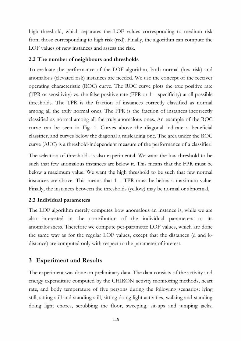
high threshold, which separates the LOF values corresponding to medium risk
from those corresponding to high risk (red). Finally, the algorithm can compute the
LOF values of new instances and assess the risk.
2.2 The number of neighbours and thresholds
To evaluate the performance of the LOF algorithm, both normal (low risk) and
anomalous (elevated risk) instances are needed. We use the concept of the receiver
operating characteristic (ROC) curve. The ROC curve plots the true positive rate
(TPR or sensitivity) vs. the false positive rate (FPR or 1 – specificity) at all possible
thresholds. The TPR is the fraction of instances correctly classified as normal
among all the truly normal ones. The FPR is the fraction of instances incorrectly
classified as normal among all the truly anomalous ones. An example of the ROC
curve can be seen in Fig. 1. Curves above the diagonal indicate a beneficial
classifier, and curves below the diagonal a misleading one. The area under the ROC
curve (AUC) is a threshold-independent measure of the performance of a classifier.
The selection of thresholds is also experimental. We want the low threshold to be
such that few anomalous instances are below it. This means that the FPR must be
below a maximum value. We want the high threshold to be such that few normal
instances are above. This means that 1 – TPR must be below a maximum value.
Finally, the instances between the thresholds (yellow) may be normal or abnormal.
2.3 Individual parameters
The LOF algorithm merely computes how anomalous an instance is, while we are
also interested in the contribution of the individual parameters to its
anomalousness. Therefore we compute per-parameter LOF values, which are done
the same way as for the regular LOF values, except that the distances (d and k-
distance) are computed only with respect to the parameter of interest.
3 Experiment and Results
The experiment was done on preliminary data. The data consists of the activity and
energy expenditure computed by the CHIRON activity monitoring methods, heart
rate, and body temperature of five persons during the following scenarios: lying
still, sitting still and standing still, sitting doing light activities, walking and standing
doing light chores, scrubbing the floor, sweeping, sit-ups and jumping jacks,
115
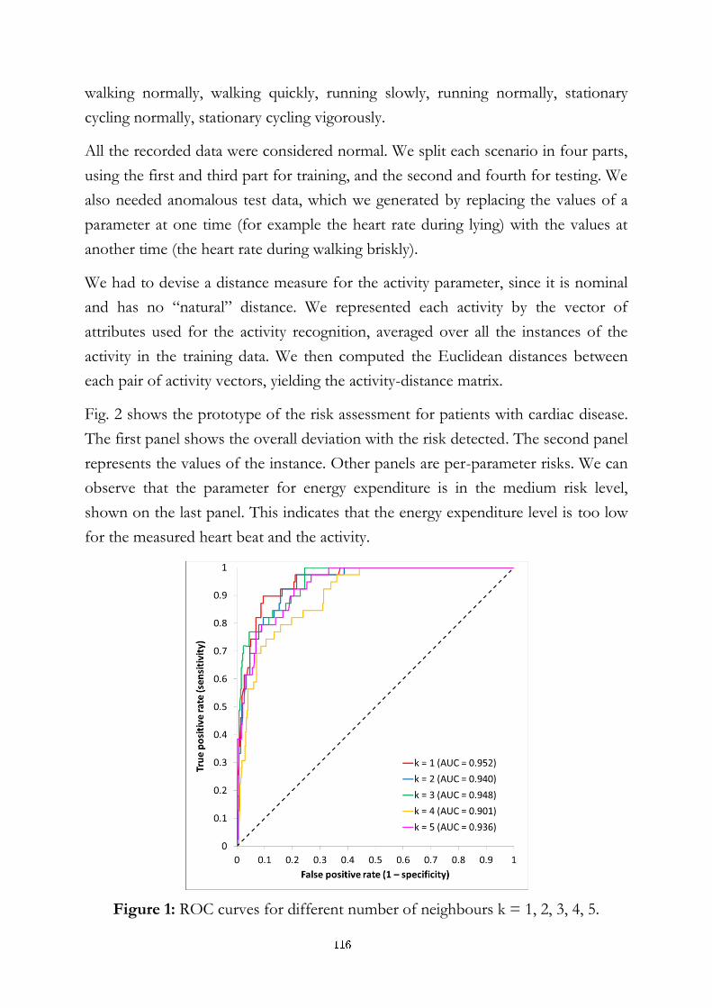
walking normally, walking quickly, running slowly, running normally, stationary
cycling normally, stationary cycling vigorously.
All the recorded data were considered normal. We split each scenario in four parts,
using the first and third part for training, and the second and fourth for testing. We
also needed anomalous test data, which we generated by replacing the values of a
parameter at one time (for example the heart rate during lying) with the values at
another time (the heart rate during walking briskly).
We had to devise a distance measure for the activity parameter, since it is nominal
and has no “natural” distance. We represented each activity by the vector of
attributes used for the activity recognition, averaged over all the instances of the
activity in the training data. We then computed the Euclidean distances between
each pair of activity vectors, yielding the activity-distance matrix.
Fig. 2 shows the prototype of the risk assessment for patients with cardiac disease.
The first panel shows the overall deviation with the risk detected. The second panel
represents the values of the instance. Other panels are per-parameter risks. We can
observe that the parameter for energy expenditure is in the medium risk level,
shown on the last panel. This indicates that the energy expenditure level is too low
for the measured heart beat and the activity.
Figure 1: ROC curves for different number of neighbours k = 1, 2, 3, 4, 5.
116
4 Conclusion
In this paper we have shown that LOF can be used for health risk assessment. We
have extended the general LOF to use nominal values in our case activity and to
show the level of abnormality.
The disadvantage of LOF as a risk assessment method is that a new pattern is not
necessarily a sign of increased risk. However, the advantage is that it can detect any
kind of anomaly – there is no need for an expert to describe the possible anomalies
and no need for examples of the anomalies (labelled data).
Figure 2: The prototype showing the anomaly detection due to the MET value.
References:
[1] M. M. Breunig,, H.-P. Kriegel, R. T. Ng & J. Sander. LOF: Identifying density-based local outliers. In Proc. of ACM SIGMOD International Conference on Management of Data, 2000.
117
For wider interest
The purpose of the medical expert systems is to disburden the workload of
physicians and ease the detection of abnormal events. Research in this field is quite
mature. However, modules that assemble the expert system are based on
predefined rules created by the expert or models trained on the labelled data. For
example, when a patient’s health is normal, the parameters characterizing it usually
follow some recurrent patterns. When the patient’s health is not normal certain
parameters move from the normal state and influence others. The rules and models
created to detect the risk are highly correlated with the disease they were created
for. This means that in case we would like to analyse a different disease, domain
new rules have to be created and models trained. For that we would need relatively
large amount of relevant labelled data.
There are four problems we are focused on in this research (i) can we use
unlabelled data, (ii) is it possible to consider individuality of the patient regarding
the pattern of vital signs and their influence to each other, (iii) can we detect the
level of the abnormality and (iv) is it possible to detect how much do the analysed
parameters contribute to the risk?
In this research we have adopted the Local Outlier Factor (LOF) algorithm, since it
seems the most appropriate method to detect the abnormal events using unlabelled
data and by that keep the individuality of the person. The algorithm was extended
with the procedure for abnormality level detection per monitored parameter. The
developed algorithm enables the doctor to see which of the monitored parameters
contribute to the overall risk at most.
The disadvantage of LOF as a risk assessment method is that a new pattern is not
necessarily a sign of increased risk. However, the advantage is that it can detect any
kind of anomaly – there is no need for an expert to describe the possible anomalies
and no need for examples of the anomalies (labelled data).
118
Diagnostika sistemov z gorivnimi celicami in izboljšanje njihovega delovanja
Andrej Debenjak1,2
1 Odsek za sisteme in vodenje, Institut »Jožef Stefan«, Ljubljana, Slovenija
2 Mednarodna podiplomska šola Jožefa Stefana, Ljubljana, Slovenija
Povzetek. Dejavniki, kot so omejene zaloge fosilnih goriv, vse večja svetovna
poraba energije in vse ostrejši okoljevarstveni predpisi, spodbujajo iskanje
novih rešitev na področju okolju prijaznega pridobivanja energije. PEM
gorivne celice so se izkazale za obetajočo tehnologijo, ki predstavlja alternativo
današnjim virom energije tako v stacionarnih kot transportnih aplikacijah
manjših moči. Največji potencial kažejo na področjih osebnega prevoza,
logistične opreme za ravnanje s transportnim blagom, zasilnih in
brezprekinitvenih napajalnih sistemih ter porazdeljene proizvodnje energije.
Kljub vsemu je za uspešen prodor tehnologije na trg potrebno rešiti še
nekatere težave, ki so povezane z zanesljivostjo delovanja PEM gorivnih celic.
Največjo še ne rešeno težavo predstavljata poplavljanje celic in izsuševanje
membran med delovanjem, ki negativno vplivajo na delovanje in v skrajnih
primerih lahko vodijo v okvare. Te napake v delovanju je mogoče učinkovito
odpravljati s pomočjo naprednih sistemov vodenja, pri čemer je odločilnega
pomena diagnostika napak, saj tako poplavljanja kot tudi izsuševanja ni
mogoče zaznati z neposrednimi meritvami.
Ključne besede: PEM gorivne celice, zanesljivost delovanja, diagnostika.
1 Uvod
Gorivne celice (GC) so elektrokemične naprave, ki kemično energijo vodika
neposredno pretvarjajo v električno in toplotno energijo. Pri delovanju se
porabljata vodik in kisik, kot edini stranski produkt pa nastaja voda, zato so GC
popolnoma čist vir energije.
V transportnih in stacionarnih aplikacijah, kjer so potrebni viri električne energije
moči do 100 kW, so se kot najprimernejše izkazale GC s protonsko prevodno
119
membrano (ang. Proton Exchange Membrane – PEM) [1]. PEM GC poleg že
opisanih lastnosti odlikujejo še nizka obratovalna temperatura, tiho delovanje in
velika gostota moči. Področja, kjer so PEM GC primerne za vgradnjo, so:
avtomobili in manjša prevozna sredstva za osebni prevoz, manjši delovni in
transportni stroji, zasilni in brezprekinitveni napajalni sistemi, porazdeljeno
sopridobivanje električne in toplotne energije ter vojaške aplikacije.
Trenutno največjo oviro masovni uporabi PEM GC predstavljajo težave povezane
z zagotavljanjem zanesljivosti delovanja [2]. Nezanesljivost je večinoma posledica
neželenih pojavov znotraj celic, ki se dogodijo med samim delovanjem. To sta
poplavljanje celic in izsuševanje PEM membran. Ti dve napaki sta nemerljivi s
standardnimi postopki, zato je za njihovo zaznavanje potrebno uporabiti
diagnostične metode. Povečanje zanesljivosti delovanja pa se doseže tako, da se
informacija, pridobljena z diagnostiko, uporabi v sklopu sistema vodenja, ki izvede
ustrezno regulacijsko akcijo z namenom odpraviti napako.
V prispevku je predstavljena elektrokemična impedančna spektroskopija (EIS), ki je
že dokazano učinkovita metoda za diagnosticiranje poplavljanja in izsuševanja
samostojnih GC ob uporabi laboratorijske merilne opreme [3, 4]. Ker pa so realni
sistemi sestavljeni iz več deset GC povezanih v serijo, ki tvorijo sklad GC, je
potrebno metodo prilagoditi, saj v tem primeru posamezne GC niso neposredno
dostopne in je potrebno metodo izvajati na celotnem skladu. Največjo s tem
povezano težavo predstavlja izredno zakrita iskana informacija, saj se napake
navadno dogodijo le znotraj nekaj celic sklada, diagnostika pa se opravlja nad
celotnim skladom.
2 Predstavitev problema
PEM gorivna celica med delovanje proizvaja vodo, ki jo je potrebno odvajati, hkrati
pa je nekaj vode potrebne za vzdrževanje ustrezne vlažnosti PEM membrane. Tako
se celica tekom delovanja neprestano nahaja med preveč prisotne vode in
pomanjkanjem vode, pri čemer je intenzivnost odvajanje vode regulirana s pomočjo
temperature in pretoka zraka [1].
V primeru, ko je odvajanje vode nezadostno, se le-ta začne kondenzirati v zračnih
kanalčkih in povzroči poplavljanje celice. Nastale kapljice vode v kanalčkih
onemogočajo dostop zraka do mesta, kjer poteka kemijska reakcija, kar povzroči
primanjkljaj reaktantov in posledično nezmožnost zagotavljanja zahtevane izhodne
120
električne moči. Navzven je to vidno kot padec izhodne napetosti in izkoristka
celice.
Protonska prevodnost PEM membrane je odvisna od vsebnosti vode v njej, zato je
potrebno neprestano zagotavljati zadostno vsebnost le-te znotraj membrane. V
primeru preobsežnega odvajanja nastale vode začne izhlapevati tudi voda iz
membrane, kar vpliva na znižanje protonske prevodnosti. To pa hkrati pomeni, da
se notranja upornost gorivne celice poveča in izhodna napetost pade. Ob tem
lahko ob dolgotrajnem in močnem izsuševanju pride tudi do fizičnih okvar PEM
membrane.
3 Uporaba EIS na sistemih s skladom gorivnih celic
EIS je elektrokemična diagnostična metoda, ki omogoča zaznavanje napak
poplavljanja in izsuševanja PEM GC. Bistvo metode predstavlja ideja, da se
posamezne napake različno manifestirajo v impedančni karakteristiki GC. To
pomeni, da je potrebno GC med delovanjem vzbujati z vsiljenim tokovnim
signalom, posneti njen napetostni odziv in izračunati njeno impedančno
karakteristiko, na podlagi katere je nato mogoče določiti, kaj se znotraj celice
dogaja.
Meritve po metodi EIS se izvedejo tako, da v določeni delovni točki (ki je določena
z bremenskim tokom) enosmerni komponenti toka superponiramo sinusni
vzbujalni signal manjše amplitude in znane frekvence [5]. Ob predpostavki, da je
sistem gorivne celice v okolici delovne točke linearen, se le-ta na sinusno vzbujanje
odzove s sinusnim napetostnim odzivom. Tokovni in napetostni signal lahko
zapišemo s pomočjo kompleksorjev.
)(
0
0
0
0
tj
tj
eUU
eII (1)
Kjer je ω0 krožna frekvenca signalov, I0 in U0 amplitudi signalov in φ fazni zamik
napetostnega odziva. Vrednost impedance Z gorivne celice pri vzbujeni krožni
frekvenci ω0 je po Ohmovem zakonu:
j
tj
tj
eZeI
eU
I
UZ 0
0
)(
0
0
0
, (2)
kjer je Z0 amplituda impedance in Φ fazni kot impedance gorivne celice pri izbrani
krožni frekvenci ω0.
121
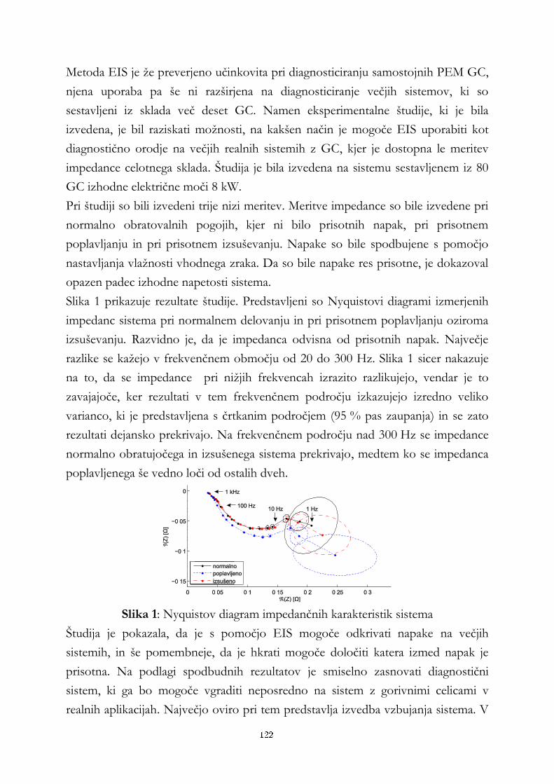
Metoda EIS je že preverjeno učinkovita pri diagnosticiranju samostojnih PEM GC,
njena uporaba pa še ni razširjena na diagnosticiranje večjih sistemov, ki so
sestavljeni iz sklada več deset GC. Namen eksperimentalne študije, ki je bila
izvedena, je bil raziskati možnosti, na kakšen način je mogoče EIS uporabiti kot
diagnostično orodje na večjih realnih sistemih z GC, kjer je dostopna le meritev
impedance celotnega sklada. Študija je bila izvedena na sistemu sestavljenem iz 80
GC izhodne električne moči 8 kW.
Pri študiji so bili izvedeni trije nizi meritev. Meritve impedance so bile izvedene pri
normalno obratovalnih pogojih, kjer ni bilo prisotnih napak, pri prisotnem
poplavljanju in pri prisotnem izsuševanju. Napake so bile spodbujene s pomočjo
nastavljanja vlažnosti vhodnega zraka. Da so bile napake res prisotne, je dokazoval
opazen padec izhodne napetosti sistema.
Slika 1 prikazuje rezultate študije. Predstavljeni so Nyquistovi diagrami izmerjenih
impedanc sistema pri normalnem delovanju in pri prisotnem poplavljanju oziroma
izsuševanju. Razvidno je, da je impedanca odvisna od prisotnih napak. Največje
razlike se kažejo v frekvenčnem območju od 20 do 300 Hz. Slika 1 sicer nakazuje
na to, da se impedance pri nižjih frekvencah izrazito razlikujejo, vendar je to
zavajajoče, ker rezultati v tem frekvenčnem področju izkazujejo izredno veliko
varianco, ki je predstavljena s črtkanim področjem (95 % pas zaupanja) in se zato
rezultati dejansko prekrivajo. Na frekvenčnem področju nad 300 Hz se impedance
normalno obratujočega in izsušenega sistema prekrivajo, medtem ko se impedanca
poplavljenega še vedno loči od ostalih dveh.
Slika 1: Nyquistov diagram impedančnih karakteristik sistema
Študija je pokazala, da je s pomočjo EIS mogoče odkrivati napake na večjih
sistemih, in še pomembneje, da je hkrati mogoče določiti katera izmed napak je
prisotna. Na podlagi spodbudnih rezultatov je smiselno zasnovati diagnostični
sistem, ki ga bo mogoče vgraditi neposredno na sistem z gorivnimi celicami v
realnih aplikacijah. Največjo oviro pri tem predstavlja izvedba vzbujanja sistema. V
122
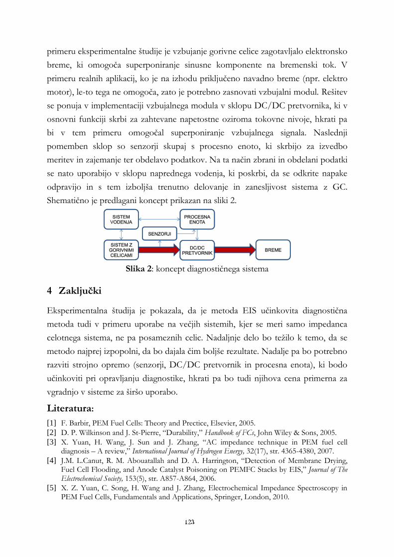
primeru eksperimentalne študije je vzbujanje gorivne celice zagotavljalo elektronsko
breme, ki omogoča superponiranje sinusne komponente na bremenski tok. V
primeru realnih aplikacij, ko je na izhodu priključeno navadno breme (npr. elektro
motor), le-to tega ne omogoča, zato je potrebno zasnovati vzbujalni modul. Rešitev
se ponuja v implementaciji vzbujalnega modula v sklopu DC/DC pretvornika, ki v
osnovni funkciji skrbi za zahtevane napetostne oziroma tokovne nivoje, hkrati pa
bi v tem primeru omogočal superponiranje vzbujalnega signala. Naslednji
pomemben sklop so senzorji skupaj s procesno enoto, ki skrbijo za izvedbo
meritev in zajemanje ter obdelavo podatkov. Na ta način zbrani in obdelani podatki
se nato uporabijo v sklopu naprednega vodenja, ki poskrbi, da se odkrite napake
odpravijo in s tem izboljša trenutno delovanje in zanesljivost sistema z GC.
Shematično je predlagani koncept prikazan na sliki 2.
Slika 2: koncept diagnostičnega sistema
4 Zaključki
Eksperimentalna študija je pokazala, da je metoda EIS učinkovita diagnostična
metoda tudi v primeru uporabe na večjih sistemih, kjer se meri samo impedanca
celotnega sistema, ne pa posameznih celic. Nadaljnje delo bo težilo k temo, da se
metodo najprej izpopolni, da bo dajala čim boljše rezultate. Nadalje pa bo potrebno
razviti strojno opremo (senzorji, DC/DC pretvornik in procesna enota), ki bodo
učinkoviti pri opravljanju diagnostike, hkrati pa bo tudi njihova cena primerna za
vgradnjo v sisteme za širšo uporabo.
Literatura:
[1] F. Barbir, PEM Fuel Cells: Theory and Prectice, Elsevier, 2005.
[2] D. P. Wilkinson and J. St-Pierre, “Durability,” Handbook of FCs, John Wiley & Sons, 2005.
[3] X. Yuan, H. Wang, J. Sun and J. Zhang, “AC impedance technique in PEM fuel cell diagnosis – A review,” International Journal of Hydrogen Energy, 32(17), str. 4365-4380, 2007.
[4] J.M. L.Canut, R. M. Abouatallah and D. A. Harrington, “Detection of Membrane Drying, Fuel Cell Flooding, and Anode Catalyst Poisoning on PEMFC Stacks by EIS,” Journal of The Electrochemical Society, 153(5), str. A857-A864, 2006.
[5] X. Z. Yuan, C. Song, H. Wang and J. Zhang, Electrochemical Impedance Spectroscopy in PEM Fuel Cells, Fundamentals and Applications, Springer, London, 2010.
123
Za širši interes
Gorivne celice so naprave, ki kemično energijo goriva (največkrat je to vodik)
neposredno pretvarjajo v električno energijo. Energija se pretvarja s pomočjo
elektrokemične reakcije, pri kateri se vodik spaja s kisikom, pri tem pa kot edini
produkt nastaja voda. Zaradi tega so gorivne celice izredno čista tehnologija za
pridobivanje električne energije.
Ob tem, da so gorivne celice okolju prijazne, jih odlikujejo tudi nekatere druge
lastnosti: ne vsebujejo nobenih premičnih ali vrtečih se delov, tihost delovanja in
visoki izkoristki. Te njihove dobre lastnosti jih delajo primerne za vgradnjo v
raznorazne aplikacije, kjer lahko nadomestijo trenutne okolju neprijazne vire
energije.
Pri aplikacijah, kjer so potrebni viri električne energije manjših moči, so se kot
najprimernejše izkazale gorivne celice s protonsko prevodno membrano (ang.
Proton Exchange Membrane – PEM). PEM gorivne celice, poleg že predstavljenih
lastnosti, dodatno odlikujejo tudi nizka obratovalna temperatura in velika gostota
moči. Področja, kjer so PEM gorivne celice primerne za uporabo, so: avtomobili in
manjša prevozna sredstva za osebni prevoz, manjši delovni in transportni stroji,
zasilni in brezprekinitveni napajalni sistemi, porazdeljeno sopridobivanje električne
in toplotne energije ter vojaške aplikacije.
Še ne odpravljene težave, ki ovirajo prodor PEM gorivnih celic na širši trg, so
povezane z zagotavljanjem zanesljivosti delovanja celic. Nezanesljivost je v največji
meri posledica napak povezanih z nastalo vodo med delovanjem in njenim
odvajanjem iz celic. Ti dve napaki sta tako imenovani poplavljanje celic in
izsuševanje PEM membran. Napaki sta nemerljivi s standardnimi postopki, zato je
za njihovo zaznavanje potrebno uporabiti diagnostične metode. Povečanje
zanesljivosti delovanja pa se doseže tako, da se informacija, pridobljena z
diagnostiko, uporabi v sklopu sistema vodenja, ki izvede ustrezno regulacijsko
akcijo z namenom odpraviti napake.
V prispevku je predstavljena elektrokemična impedančna spektroskopija, ki je bila
uporabljena za diagnosticiranje napak tekom delovanja. Hkrati pa je podan tudi
koncept za implementacijo metode znotraj sistema vodenja gorivnih celic, ki
poskrbi za odpravo napak in ustreznost delovanja.
124
Risk Assessment Model for Congestive Heart Failure
Hristijan Gjoreski1,2
1 Department of Intelligent Systems, Jožef Stefan Institute, Ljubljana, Slovenia
2 Jožef Stefan International Postgraduate School, Ljubljana, Slovenia
Abstract. Congestive heart failure is a common, chronic and debilitating
condition with an extremely poor prognosis. This paper presents an approach
to creation of risk assessment model for congestive heart failure. Two types of
hierarchical multi-attribute models are developed and compared: qualitative
and quantitative. The results for both models showed that the models can
successfully assist and help the experts in their decision for estimation of the
patient's risk. Also, the models analysis techniques can assist additionally by
giving advices for future improvement of patient's health.
Keywords: Congestive heart failure, Risk assessment model, Decision
support, Expert system.
1 Introduction
Congestive heart failure (CHF) is a common, chronic and debilitating condition. It
is an issue when the heart cannot pump enough blood to the rest of the body. It is
more common than most cancers, including breast, testicular, cervical and bowel
cancers. Approximately 14 million people suffer from CHF in Europe [1].
The CHF issue is addressed in the CHIRON project [2]. The CHIRON is a
European project whose final goal is the development of a reference architecture
for personal elderly healthcare. One of the modules of the project is the creation of
CHF Risk Assessment Model (RAM), which should assist the doctors in assessing
the CHF risk of a patient. The aim of the RAM is to provide to the doctors the
information needed to make clinical decisions regarding the patient’s health.
In this paper we describe the development of a long-term RAM for CHF. Two
approaches were used: qualitative and quantitative. Additionally, for both RAMs a
125
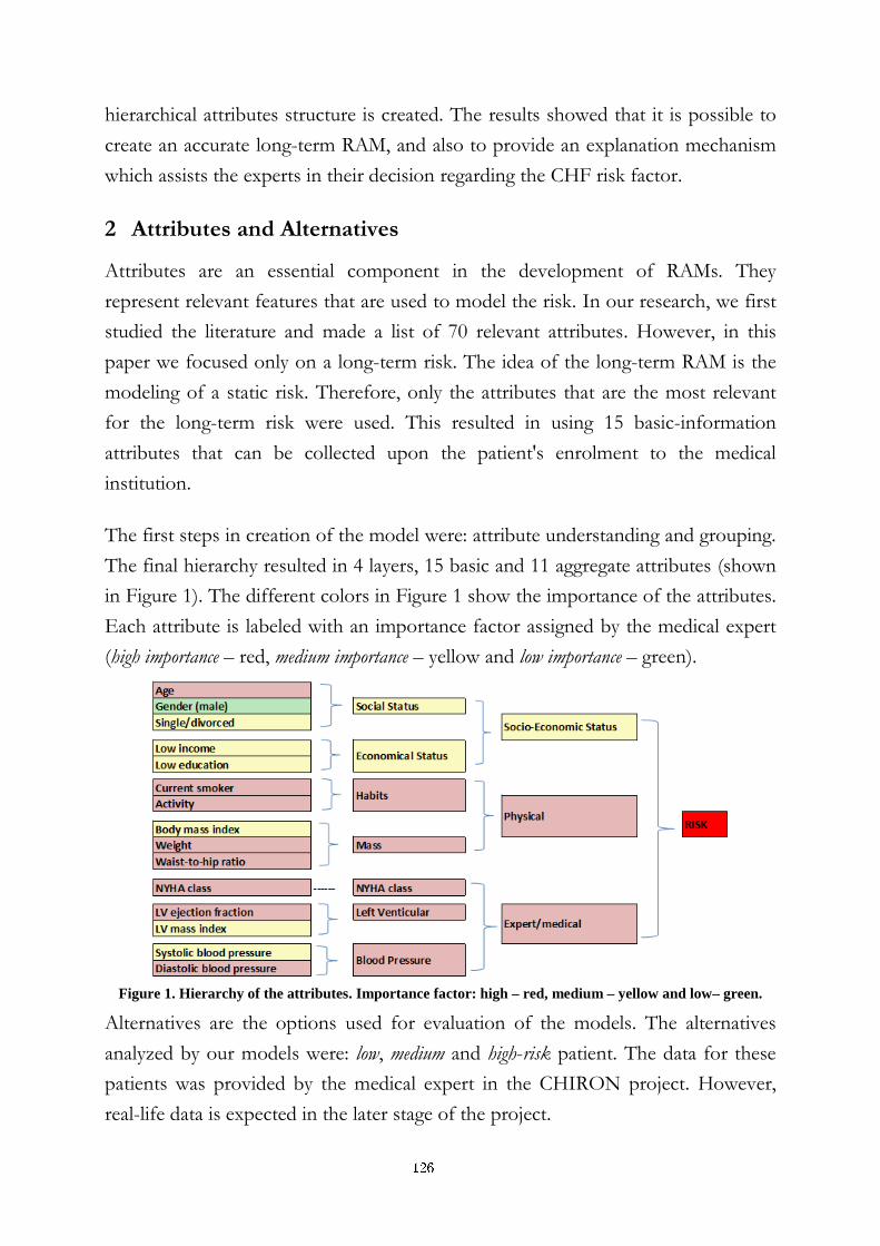
hierarchical attributes structure is created. The results showed that it is possible to
create an accurate long-term RAM, and also to provide an explanation mechanism
which assists the experts in their decision regarding the CHF risk factor.
2 Attributes and Alternatives
Attributes are an essential component in the development of RAMs. They
represent relevant features that are used to model the risk. In our research, we first
studied the literature and made a list of 70 relevant attributes. However, in this
paper we focused only on a long-term risk. The idea of the long-term RAM is the
modeling of a static risk. Therefore, only the attributes that are the most relevant
for the long-term risk were used. This resulted in using 15 basic-information
attributes that can be collected upon the patient's enrolment to the medical
institution.
The first steps in creation of the model were: attribute understanding and grouping.
The final hierarchy resulted in 4 layers, 15 basic and 11 aggregate attributes (shown
in Figure 1). The different colors in Figure 1 show the importance of the attributes.
Each attribute is labeled with an importance factor assigned by the medical expert
(high importance – red, medium importance – yellow and low importance – green).
Figure 1. Hierarchy of the attributes. Importance factor: high – red, medium – yellow and low– green.
Alternatives are the options used for evaluation of the models. The alternatives
analyzed by our models were: low, medium and high-risk patient. The data for these
patients was provided by the medical expert in the CHIRON project. However,
real-life data is expected in the later stage of the project.
126
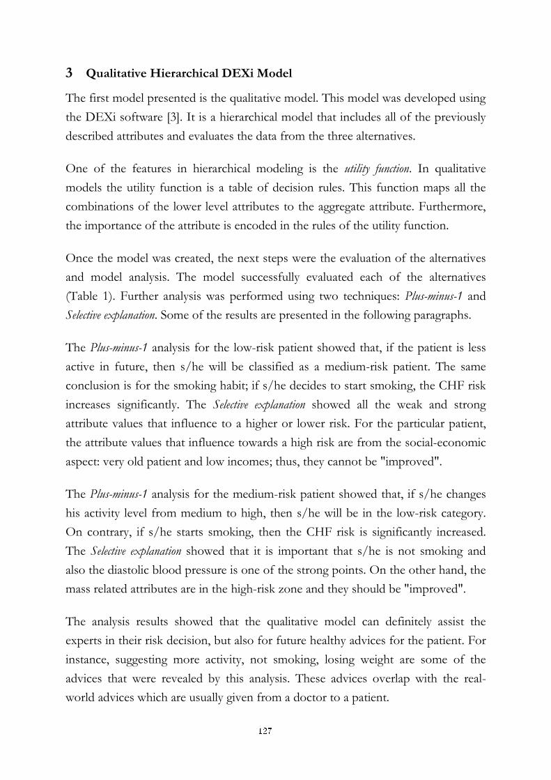
3 Qualitative Hierarchical DEXi Model
The first model presented is the qualitative model. This model was developed using
the DEXi software [3]. It is a hierarchical model that includes all of the previously
described attributes and evaluates the data from the three alternatives.
One of the features in hierarchical modeling is the utility function. In qualitative
models the utility function is a table of decision rules. This function maps all the
combinations of the lower level attributes to the aggregate attribute. Furthermore,
the importance of the attribute is encoded in the rules of the utility function.
Once the model was created, the next steps were the evaluation of the alternatives
and model analysis. The model successfully evaluated each of the alternatives
(Table 1). Further analysis was performed using two techniques: Plus-minus-1 and
Selective explanation. Some of the results are presented in the following paragraphs.
The Plus-minus-1 analysis for the low-risk patient showed that, if the patient is less
active in future, then s/he will be classified as a medium-risk patient. The same
conclusion is for the smoking habit; if s/he decides to start smoking, the CHF risk
increases significantly. The Selective explanation showed all the weak and strong
attribute values that influence to a higher or lower risk. For the particular patient,
the attribute values that influence towards a high risk are from the social-economic
aspect: very old patient and low incomes; thus, they cannot be "improved".
The Plus-minus-1 analysis for the medium-risk patient showed that, if s/he changes
his activity level from medium to high, then s/he will be in the low-risk category.
On contrary, if s/he starts smoking, then the CHF risk is significantly increased.
The Selective explanation showed that it is important that s/he is not smoking and
also the diastolic blood pressure is one of the strong points. On the other hand, the
mass related attributes are in the high-risk zone and they should be "improved".
The analysis results showed that the qualitative model can definitely assist the
experts in their risk decision, but also for future healthy advices for the patient. For
instance, suggesting more activity, not smoking, losing weight are some of the
advices that were revealed by this analysis. These advices overlap with the real-
world advices which are usually given from a doctor to a patient.
127
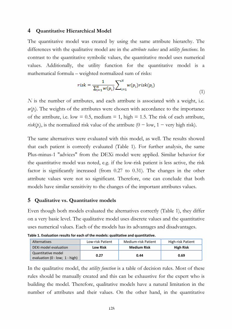
4 Quantitative Hierarchical Model
The quantitative model was created by using the same attribute hierarchy. The
differences with the qualitative model are in the attribute values and utility functions. In
contrast to the quantitative symbolic values, the quantitative model uses numerical
values. Additionally, the utility function for the quantitative model is a
mathematical formula – weighted normalized sum of risks:
(1)
N is the number of attributes, and each attribute is associated with a weight, i.e.
w(pi). The weights of the attributes were chosen with accordance to the importance
of the attribute, i.e. low = 0.5, medium = 1, high = 1.5. The risk of each attribute,
risk(pi), is the normalized risk value of the attribute (0 − low, 1 − very high risk).
The same alternatives were evaluated with this model, as well. The results showed
that each patient is correctly evaluated (Table 1). For further analysis, the same
Plus-minus-1 "advices" from the DEXi model were applied. Similar behavior for
the quantitative model was noted, e.g. if the low-risk patient is less active, the risk
factor is significantly increased (from 0.27 to 0.31). The changes in the other
attribute values were not so significant. Therefore, one can conclude that both
models have similar sensitivity to the changes of the important attributes values.
5 Qualitative vs. Quantitative models
Even though both models evaluated the alternatives correctly (Table 1), they differ
on a very basic level. The qualitative model uses discrete values and the quantitative
uses numerical values. Each of the models has its advantages and disadvantages.
Table 1. Evaluation results for each of the models: qualitative and quantitative.
Alternatives Low-risk Patient Medium-risk Patient High-risk Patient
DEXi model evaluation Low Risk Medium Risk High Risk
Quantitative model evaluation (0 - low; 1 - high)
0.27 0.44 0.69
In the qualitative model, the utility function is a table of decision rules. Most of these
rules should be manually created and this can be exhaustive for the expert who is
building the model. Therefore, qualitative models have a natural limitation in the
number of attributes and their values. On the other hand, in the quantitative
128
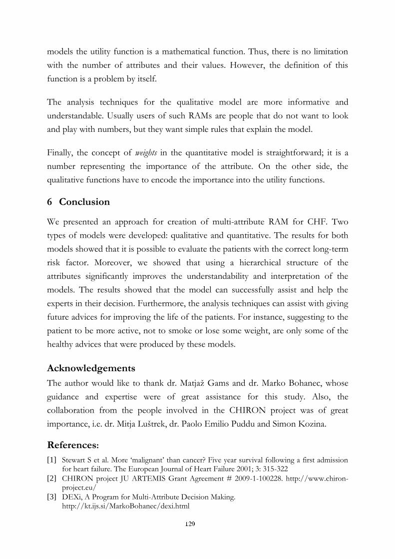
models the utility function is a mathematical function. Thus, there is no limitation
with the number of attributes and their values. However, the definition of this
function is a problem by itself.
The analysis techniques for the qualitative model are more informative and
understandable. Usually users of such RAMs are people that do not want to look
and play with numbers, but they want simple rules that explain the model.
Finally, the concept of weights in the quantitative model is straightforward; it is a
number representing the importance of the attribute. On the other side, the
qualitative functions have to encode the importance into the utility functions.
6 Conclusion
We presented an approach for creation of multi-attribute RAM for CHF. Two
types of models were developed: qualitative and quantitative. The results for both
models showed that it is possible to evaluate the patients with the correct long-term
risk factor. Moreover, we showed that using a hierarchical structure of the
attributes significantly improves the understandability and interpretation of the
models. The results showed that the model can successfully assist and help the
experts in their decision. Furthermore, the analysis techniques can assist with giving
future advices for improving the life of the patients. For instance, suggesting to the
patient to be more active, not to smoke or lose some weight, are only some of the
healthy advices that were produced by these models.
Acknowledgements
The author would like to thank dr. Matjaž Gams and dr. Marko Bohanec, whose
guidance and expertise were of great assistance for this study. Also, the
collaboration from the people involved in the CHIRON project was of great
importance, i.e. dr. Mitja Luštrek, dr. Paolo Emilio Puddu and Simon Kozina.
References:
[1] Stewart S et al. More ‘malignant’ than cancer? Five year survival following a first admission for heart failure. The European Journal of Heart Failure 2001; 3: 315-322
[2] CHIRON project JU ARTEMIS Grant Agreement # 2009-1-100228. http://www.chiron-project.eu/
[3] DEXi, A Program for Multi-Attribute Decision Making. http://kt.ijs.si/MarkoBohanec/dexi.html
129
For wider interest
Congestive heart failure (CHF) is a common and chronic condition with an
extremely poor prognosis. It is an issue when the heart cannot pump enough blood
to the rest of the body. It is more common than most cancers, including breast,
testicular, cervical and bowel cancers. Approximately 14 million people suffer from
CHF in Europe.
In this paper we presented models that can predict the CHF risk of a patient. We
were focused on predicting the long-term, static, risk that can be assessed upon
patient's enrolment in the medical institution. The aim of the model was to predict
the CHF risk, but also to provide additional explanation for the decision: the
reason why the predicted risk is such as it is (low, medium or high).
To achieve this goal, we developed two types of hierarchical models: qualitative and
quantitative. The first one is more user-friendly because it is using symbolic values
for the data, e.g. low activity, high blood pressure, medium risk, etc. The other one
is more mathematical and is using numbers instead of symbolic values.
We tested these models on a data created by a medical expert. First, the data is used
as input to the models. Then, the models analyze the data and make the final
decision (prognosis) for the risk. Additionally, both models have visualization
mechanism, which shows the attributes that are extremes: the most and the least
risky. Finally, the analysis techniques reveal healthy advices for the patient, such as:
suggesting being more active, not to smoke and lose weight.
The results showed that the models successfully predict the correct risk factor, and
also provide explanation mechanism which could assist the experts in their decision
regarding the CHF risk factor.
130
Prototip sistema za sprotni nadzor stanja industrijske opreme
Matic Ivanovič1,2, Đani Juričić1,2,3,4
1 Odsek za sisteme in vodenje, Institut "Jožef Stefan, Ljubljana", Slovenija
2 Mednarodna podiplomska šola Jožefa Stefana, Ljubljana, Slovenija
3 Univerza v Novi Gorici, Nova Gorica, Slovenija
4 Univerza v Mariboru, Maribor, Slovenija
Povzetek. V prispevku je predstavljen konceptualno nov sistem za sprotni
nadzor stanja industrijske opreme, ki ga odlikujejo nizka cena, enostavna
namestitev ter prilagodljivost različnim področjem uporabe. Ključna
komponenta sistema je pametno senzorsko vozlišče, ki je sposobno zbirati
signale iz lokalnih senzorjev, lokalno shranjevati poteke, le-te tudi lokalno
obdelati s sodobnimi postopki ter rezultate brezžično poslati na oddaljen
strežnik. Posebnost sistema je, da lahko lokalne postopke obdelave signalov
poljubno spreminjamo kar na daljavo preko brezžičnega omrežja. Celotna
aplikacija se razvije v Simulinku, ki predstavlja standardno orodje za
načrtovanje, in se nato s posebno izdelanim programom avtomatsko prevede v
obliko, primerno za ciljni procesor v vozlišču. Delovanje prototipa pametnega
senzorskega vozlišča ter okolja za konfiguracijo smo preizkusili tudi na
preprosti aplikaciji in pokazali, da je možno izdelati cenovno ugoden in
zmogljiv sistem za sprotni nadzor stanja opreme.
Ključne besede: diagnostika, sprotni nadzor stanja, senzorsko vozlišče
1 Uvod
Sprotni avtomatiziran nadzor stanja opreme predstavlja pomemben trend v novih
generacijah sistemov za avtomatsko vodenje procesov. Današnji postopki
vzdrževanja procesne opreme so žal večinoma reaktivni (post-mortem), v
najboljšem primeru pa preventivni. Napredno in ekonomsko bolj učinkovito
prediktivno vzdrževanje pa se uporablja le v novejših in razmeroma kompleksnih
aplikacijah. Prediktivno vzdrževanje temelji na naprednih postopkih diagnostike,
131

prognostike in upravljanja vzdrževanja (angl. prognostics and health management,
PHM), ki se nanašajo na napovedovanje preostale življenjske dobe komponent ter
odločanje o vzdrževalnih posegih za zagotavljanje normalnega obratovanja naprav.
Razlogi za majhno prisotnost prediktivnega vzdrževanja v industriji so predvsem
visoka cena, zahtevna namestitev [1], pri tem pa so obstoječi nadzorni sistemi
narejeni le za specifične aplikacije in jih ni možno enostavno prenesti na druge,
podobne sisteme. Zato smo se odločili, da zgradimo dovolj splošno platformo s
katero bi se izognili omenjenim slabostim.
Zgradbo nadzornega sistema lahko razdelimo na več nivojev. Na najnižjem nivoju
so na posameznih mehanskih sklopih nameščeni različni senzorji. Povezani so na
eno ali več manjših naprav, t. i. senzorska vozlišča, ki vršijo osnovno obdelavo
izmerjenih podatkov in rezultate s pomočjo brezžičnih tehnologij pošiljajo na
strežnik. Tu se vrši nadaljnja obdelava prejetih podatkov in shranjevanje v
podatkovno bazo. Prav tako lahko preko strežnika razvijalec določa lastnosti
senzorskega omrežja in nastavlja delovanje posameznih naprav v omrežju. Na
najvišjem nivoju je zgrajen uporabniški vmesnik, ki upravljavcem omogoča vpogled
v podatke o posameznih nadzorovanih napravah. Uporabniku je na voljo ocena
trenutnega stanja naprave ter napoved preostale življenjske dobe naprave [2], [3].
Na podlagi teh podatkov se lahko upravljavci odločijo o morebitnih vzdrževalnih
posegih.
V prispevku smo se omejili na predstavitev senzorskega vozlišča ter okolja za
načrtovanje postopkov za obdelavo signalov na posameznih vozliščih. Opisan je
tudi preizkus delovanja na preprostem eksperimentalnem sistemu.
2 Pametno senzorsko vozlišče
Pametno senzorsko vozlišče je osnovni gradnik nadzornega sistema. Gre za
samostojno napravo, ki je sestavljena iz mikrokrmilnika, različnih senzorjev,
komunikacijskega vmesnika ter napajalnega modula in po potrebi tudi dodatnega
spomina. Slika 1 prikazuje blokovno shemo vozlišča z dejanskimi komponentami,
ki smo jih uporabili pri izgradnji prototipa senzorskega vozlišča. Uporabili smo
Atmelov mikrokrmilnik ATXMEGA32A4. Za analogno-digitalno pretvorbo signala
iz senzorjev smo uporabili kar analogno-digitalni pretvornik (angl. analog-to-digital
132
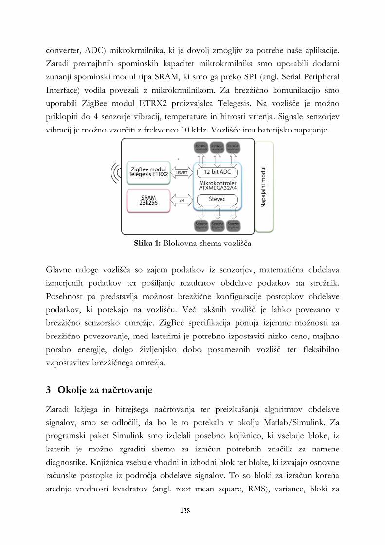
converter, ADC) mikrokrmilnika, ki je dovolj zmogljiv za potrebe naše aplikacije.
Zaradi premajhnih spominskih kapacitet mikrokrmilnika smo uporabili dodatni
zunanji spominski modul tipa SRAM, ki smo ga preko SPI (angl. Serial Peripheral
Interface) vodila povezali z mikrokrmilnikom. Za brezžično komunikacijo smo
uporabili ZigBee modul ETRX2 proizvajalca Telegesis. Na vozlišče je možno
priklopiti do 4 senzorje vibracij, temperature in hitrosti vrtenja. Signale senzorjev
vibracij je možno vzorčiti z frekvenco 10 kHz. Vozlišče ima baterijsko napajanje.
Slika 1: Blokovna shema vozlišča
Glavne naloge vozlišča so zajem podatkov iz senzorjev, matematična obdelava
izmerjenih podatkov ter pošiljanje rezultatov obdelave podatkov na strežnik.
Posebnost pa predstavlja možnost brezžične konfiguracije postopkov obdelave
podatkov, ki potekajo na vozlišču. Več takšnih vozlišč je lahko povezano v
brezžično senzorsko omrežje. ZigBee specifikacija ponuja izjemne možnosti za
brezžično povezovanje, med katerimi je potrebno izpostaviti nizko ceno, majhno
porabo energije, dolgo življenjsko dobo posameznih vozlišč ter fleksibilno
vzpostavitev brezžičnega omrežja.
3 Okolje za načrtovanje
Zaradi lažjega in hitrejšega načrtovanja ter preizkušanja algoritmov obdelave
signalov, smo se odločili, da bo le to potekalo v okolju Matlab/Simulink. Za
programski paket Simulink smo izdelali posebno knjižnico, ki vsebuje bloke, iz
katerih je možno zgraditi shemo za izračun potrebnih značilk za namene
diagnostike. Knjižnica vsebuje vhodni in izhodni blok ter bloke, ki izvajajo osnovne
računske postopke iz področja obdelave signalov. To so bloki za izračun korena
srednje vrednosti kvadratov (angl. root mean square, RMS), variance, bloki za
133

detekcijo ovojnice, za filtriranje ter za izračun hitre Fourierjeve transformacije
signala.
Vsaka shema je lahko sestavljena iz vhodnih blokov, ki predstavljajo vhode za
podatke iz senzorjev. Izhodni bloki predstavljajo značilke. Z vmesnimi bloki pa so
definirani postopki za izračun želenih značilk. Skupno število vseh blokov je
pogojeno s količino pomnilnika na mikrokrmilniku, ki pa ga je možno nadgraditi.
Pri povezavi posameznih blokov v verigo je potrebno paziti na to, ali je vhod
oziroma izhod bloka vektor ali skalar. Na sliki 2 je prikazana zelo preprosta shema.
Slika 2: Primer sheme, zgrajene v programu Simulink
Funkcionalnost kakršnekoli delujoče sheme je potrebno prenesti na senzorsko
vozlišče. Za ta namen smo v Matlabu napisali posebno funkcijo, ki vse potrebne
podatke iz Simulink sheme zapiše v datoteko, katero lahko pošljemo na senzorsko
vozlišče. Seveda smo morali temu primerno prilagoditi tudi program za senzorsko
vozlišče, tako da podpira vse bloke iz Simulink knjižnice in omogoča izračun
značilk, kot je definirano v izvorni Simulink shemi. Karakteristični podatki sheme
so vrsta posameznih blokov, ki določa katero opravilo opravlja blok, in povezave
med posameznimi bloki, ki določajo vrstni red izvajanja. Nekaterim blokom je
potrebno definirati tudi parametre, ki narekujejo njihovo delovanje. Blokom za
filtriranje je potrebno podati koeficiente prenosne funkcije izbranega filtra, blokom
za izračun Fourierjeve transformacije pa število vzorcev za izračun. Ostali bloki za
svoje delovanje ne potrebujejo posebnih parametrov.
4 Preizkus delovanja
Delovanje smo preizkusili na eksperimentalnem sistemu (Slika 3) in prikazali
osnovni princip delovanja, na katerem lahko temelji nadzorni sistem za mehanske
pogone. Na vozlišče smo priključili senzor vibracij, le-ta pa je bil fiksiran na izvor
134
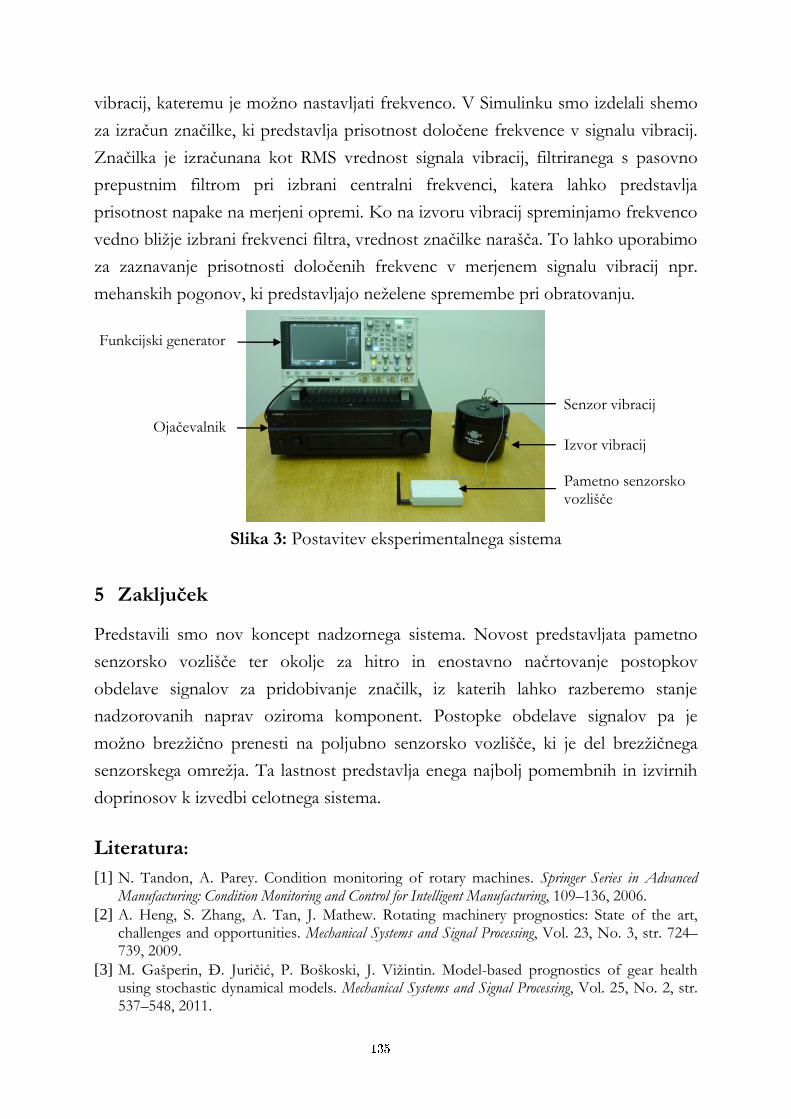
vibracij, kateremu je možno nastavljati frekvenco. V Simulinku smo izdelali shemo
za izračun značilke, ki predstavlja prisotnost določene frekvence v signalu vibracij.
Značilka je izračunana kot RMS vrednost signala vibracij, filtriranega s pasovno
prepustnim filtrom pri izbrani centralni frekvenci, katera lahko predstavlja
prisotnost napake na merjeni opremi. Ko na izvoru vibracij spreminjamo frekvenco
vedno bližje izbrani frekvenci filtra, vrednost značilke narašča. To lahko uporabimo
za zaznavanje prisotnosti določenih frekvenc v merjenem signalu vibracij npr.
mehanskih pogonov, ki predstavljajo neželene spremembe pri obratovanju.
Slika 3: Postavitev eksperimentalnega sistema
5 Zaključek
Predstavili smo nov koncept nadzornega sistema. Novost predstavljata pametno
senzorsko vozlišče ter okolje za hitro in enostavno načrtovanje postopkov
obdelave signalov za pridobivanje značilk, iz katerih lahko razberemo stanje
nadzorovanih naprav oziroma komponent. Postopke obdelave signalov pa je
možno brezžično prenesti na poljubno senzorsko vozlišče, ki je del brezžičnega
senzorskega omrežja. Ta lastnost predstavlja enega najbolj pomembnih in izvirnih
doprinosov k izvedbi celotnega sistema.
Literatura:
[1] N. Tandon, A. Parey. Condition monitoring of rotary machines. Springer Series in Advanced Manufacturing: Condition Monitoring and Control for Intelligent Manufacturing, 109–136, 2006.
[2] A. Heng, S. Zhang, A. Tan, J. Mathew. Rotating machinery prognostics: State of the art, challenges and opportunities. Mechanical Systems and Signal Processing, Vol. 23, No. 3, str. 724–739, 2009.
[3] M. Gašperin, Đ. Juričić, P. Boškoski, J. Vižintin. Model-based prognostics of gear health using stochastic dynamical models. Mechanical Systems and Signal Processing, Vol. 25, No. 2, str. 537–548, 2011.
Funkcijski generator
Ojačevalnik
Senzor vibracij
Pametno senzorsko vozlišče
Izvor vibracij
135

Za širši interes
Sprotni avtomatiziran nadzor stanja opreme predstavlja pomemben trend v novih
generacijah sistemov za avtomatsko vodenje procesov. Današnji postopki
vzdrževanja procesne opreme so žal večinoma reaktivni (post-mortem), v
najboljšem primeru pa preventivni. Napredno in ekonomsko bolj učinkovito
prediktivno vzdrževanje pa se uporablja le v novejših in razmeroma kompleksnih
aplikacijah. Prediktivno vzdrževanje temelji na naprednih postopkih diagnostike,
prognostike in upravljanja vzdrževanja (angl. prognostics and health management,
PHM), ki se nanašajo na napovedovanje preostale življenjske dobe komponent ter
odločanje o vzdrževalnih posegih za zagotavljanje normalnega obratovanja naprav.
Razlogi za majhno prisotnost prediktivnega vzdrževanja v industriji so predvsem
visoka cena, zahtevna namestitev, pri tem pa so obstoječi nadzorni sistemi narejeni
le za specifične aplikacije in jih ni možno enostavno prenesti na druge, podobne
sisteme. Naš cilj je izdelati dovolj splošno platformo za sprotni nadzor stanja
opreme s katero bi se izognili omenjenim slabostim.
136
IPSSC: Integration of structured expert knowledge
Vladimir Kuzmanovski1, 2, Sašo Džeroski1, 2, Marko Debeljak1, 2
1 Department of Knowledge Technologies, Jožef Stefan Institute, Ljubljana,
Slovenia
2 Jožef Stefan International Postgraduate School, Ljubljana, Slovenia
Abstract. This paper presents an effective implementation of data pre-
processing methodology and data mining referring to integrate decision rules
as part of manually written expert system (expert knowledge) with models
inducted from data. The methods we have used are standard methods for data
pre-processing, including techniques for handling missing data, feature
construction, transformation and aggregation, and J48 machine learning
algorithm, implemented in WEKA data mining tool set for the process of
integration of the manually created expert rules given in decision tables.
Keywords: Data Pre-processing, Data mining, Decision trees, Expert systems
1 Background & Objectives
Decades ago, scientists started with some initial algorithms for knowledge
discovery in market data that in the course of time were upgraded to satisfy new
amount of data, new types of data and to be able to be implemented in various
disciplines, such as environmental sciences, biology, medicine, etc. So, it was not
enough only to find some kind of way to discover knowledge from data, but it is
also important to update and upgrade the discipline for new type of problems.
Having this in mind, we will integrate existing expert knowledge in a form of
manually written rules which are given in decision tables with data mining. Such
integrated models will present the base unites (modules) from which the decision
support system will be structured.
The expert knowledge is already structured into manually built expert system
owned by ARVALIS Institute. It is implemented to assess the risk of pesticide
leaching from crop production. In fact, the expert system is a composition of
137
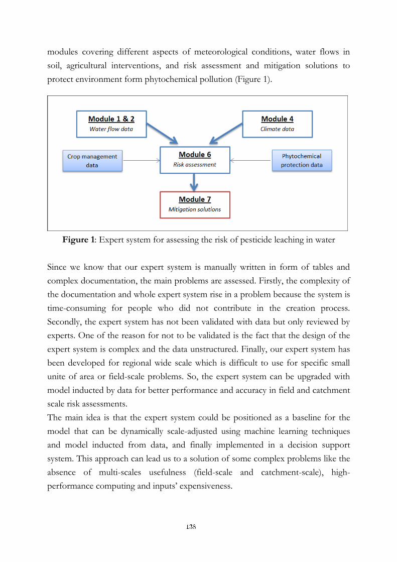
modules covering different aspects of meteorological conditions, water flows in
soil, agricultural interventions, and risk assessment and mitigation solutions to
protect environment form phytochemical pollution (Figure 1).
Figure 1: Expert system for assessing the risk of pesticide leaching in water
Since we know that our expert system is manually written in form of tables and
complex documentation, the main problems are assessed. Firstly, the complexity of
the documentation and whole expert system rise in a problem because the system is
time-consuming for people who did not contribute in the creation process.
Secondly, the expert system has not been validated with data but only reviewed by
experts. One of the reason for not to be validated is the fact that the design of the
expert system is complex and the data unstructured. Finally, our expert system has
been developed for regional wide scale which is difficult to use for specific small
unite of area or field-scale problems. So, the expert system can be upgraded with
model inducted by data for better performance and accuracy in field and catchment
scale risk assessments.
The main idea is that the expert system could be positioned as a baseline for the
model that can be dynamically scale-adjusted using machine learning techniques
and model inducted from data, and finally implemented in a decision support
system. This approach can lead us to a solution of some complex problems like the
absence of multi-scales usefulness (field-scale and catchment-scale), high-
performance computing and inputs’ expensiveness.
138
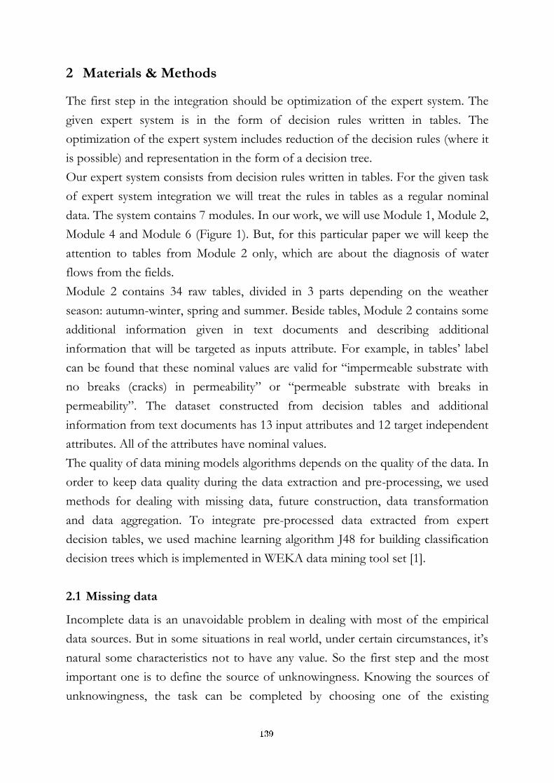
2 Materials & Methods
The first step in the integration should be optimization of the expert system. The
given expert system is in the form of decision rules written in tables. The
optimization of the expert system includes reduction of the decision rules (where it
is possible) and representation in the form of a decision tree.
Our expert system consists from decision rules written in tables. For the given task
of expert system integration we will treat the rules in tables as a regular nominal
data. The system contains 7 modules. In our work, we will use Module 1, Module 2,
Module 4 and Module 6 (Figure 1). But, for this particular paper we will keep the
attention to tables from Module 2 only, which are about the diagnosis of water
flows from the fields.
Module 2 contains 34 raw tables, divided in 3 parts depending on the weather
season: autumn-winter, spring and summer. Beside tables, Module 2 contains some
additional information given in text documents and describing additional
information that will be targeted as inputs attribute. For example, in tables’ label
can be found that these nominal values are valid for “impermeable substrate with
no breaks (cracks) in permeability” or “permeable substrate with breaks in
permeability”. The dataset constructed from decision tables and additional
information from text documents has 13 input attributes and 12 target independent
attributes. All of the attributes have nominal values.
The quality of data mining models algorithms depends on the quality of the data. In
order to keep data quality during the data extraction and pre-processing, we used
methods for dealing with missing data, future construction, data transformation
and data aggregation. To integrate pre-processed data extracted from expert
decision tables, we used machine learning algorithm J48 for building classification
decision trees which is implemented in WEKA data mining tool set [1].
2.1 Missing data
Incomplete data is an unavoidable problem in dealing with most of the empirical
data sources. But in some situations in real world, under certain circumstances, it’s
natural some characteristics not to have any value. So the first step and the most
important one is to define the source of unknowingness. Knowing the sources of
unknowingness, the task can be completed by choosing one of the existing
139

methods for handling missing data [2], [3]. We used the method for ignoring
instances with unknown feature values because we need to build a model that will
satisfy the threshold of 100% correctly classified instances over the training data.
Our task is not to make a classification model for unknown cases, but to make a
model which will cover all combinations of rules from the expert decision tables.
2.2 Feature construction, transformation and aggregation
Future subset selection, construction and transformation are the process of
identifying and removing as much irrelevant and redundant information as
possible. This may reduce the dimensionality of the data, but may allow learning
algorithms to operate faster and more effectively. Furthermore, the problem of
information mining among the data available can be addressed by constructing new
attributes from the basic future set. Transformed attributes generated by attribute
construction may provide a better discriminative ability than the best subset of
given attributes [3]. In addition, the discovery of meaningful attributes may
contribute in better understanding of the learned concept.
2.3 Classification decision trees
Decision trees are a classic way to represent information from a machine learning
algorithm, and offer a fast and powerful way to express structures in data.
According to the problem at hand and type of a given data, we used J48 algorithm
for inducing classification decision trees. J48 is a version of an earlier algorithm
developed by J. Ross Quinlan, the popular C4.5 [1].
3 Results & Discussion
In the process of integration, the total 12 classification decision trees were built,
one for each target attribute. Here we will describe the decision tree model for
“transfer by drainage” which refers to the water transfer in drainage pipes which
are buried under the fields.
The top most attribute in the drainage model (Figure 2) is “season” which splits the
model according its values “autumn and winter” and “spring and summer”. The
followed attributes “the slope of the soil” and “the presence of shrinkage cracks in
140
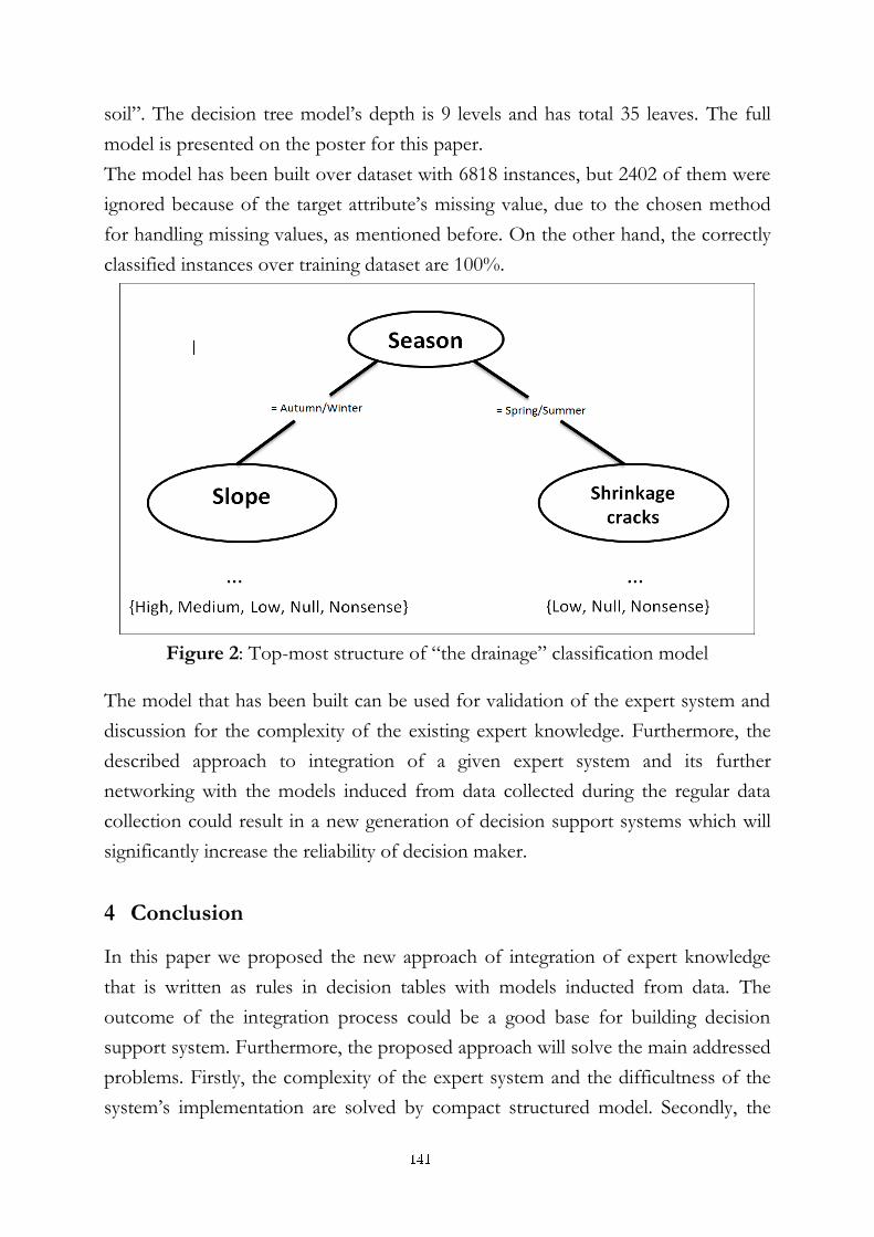
soil”. The decision tree model’s depth is 9 levels and has total 35 leaves. The full
model is presented on the poster for this paper.
The model has been built over dataset with 6818 instances, but 2402 of them were
ignored because of the target attribute’s missing value, due to the chosen method
for handling missing values, as mentioned before. On the other hand, the correctly
classified instances over training dataset are 100%.
Figure 2: Top-most structure of “the drainage” classification model
The model that has been built can be used for validation of the expert system and
discussion for the complexity of the existing expert knowledge. Furthermore, the
described approach to integration of a given expert system and its further
networking with the models induced from data collected during the regular data
collection could result in a new generation of decision support systems which will
significantly increase the reliability of decision maker.
4 Conclusion
In this paper we proposed the new approach of integration of expert knowledge
that is written as rules in decision tables with models inducted from data. The
outcome of the integration process could be a good base for building decision
support system. Furthermore, the proposed approach will solve the main addressed
problems. Firstly, the complexity of the expert system and the difficultness of the
system’s implementation are solved by compact structured model. Secondly, the
141

validation of the expert knowledge with data is done by validating the built model.
Finally, the adjustment to the field and catchment scale diagnosis has been
addressed as further work on the decision support system.
References:
[1] I. H. Witten and E. Frank. Data Mining: Practical machine learning tools and techniques, 2nd Edition. Morgan Kaufmann, 2005.
[2] Arnaud Ragel & Bruno Cremilleux. Treatment of Missing Values for Association Rules, p. 258.
[3] S. B. Kotsianitis, D. Kanellopoulos & P. E. Pintelas. Data Pre-processing for Supervised Leaning, 2006
142

For wider interest
Discovering knowledge in data or data mining becomes a very important discipline
as part of information technologies. It helps people, companies and even whole
businesses to use their own data in very practical way by finding interesting and
sometimes scientifically approved patterns and knowledge. Basically, the value of
information is always proportional to the scale of the problem it addresses.
Learning from the data and especially combine the learned patterns and knowledge
in decision support system will significantly increase the reliability of decision
maker and will produce a better support in decision making process.
The next generation of improvements of decision support systems will cover the
expert knowledge integration. We proposed an approach of integration of expert
knowledge with models inducted from data into final decision support system by
integration of expert knowledge (expert system) with data mining algorithms.
143
VESNA based platform for spectrum sensing in ISM bands
Zoltan Padrah1,2, Tomaž Šolc1, Mihael Mohorčič1,2
1 Department of Communication Systems, Jožef Stefan Institute, Ljubljana, Slovenia
2 Jožef Stefan International Postgraduate School, Ljubljana, Slovenia
Abstract. The radio spectrum used by wireless communication systems is
becoming increasingly crowded. One approach to overcome this problem is to
perform real-time dynamic spectrum assignment. To this end, it is necessary to
collect information about the radio spectrum, also called spectrum sensing. In
this paper a framework is presented which can be used for collecting
information about radio spectrum usage. This framework is based on the low-
cost and versatile VESNA sensor platform. A spectrum sensing experiment
has been performed in the 2.4 GHz to demonstrate the capabilities of the
framework.
Keywords: spectrum sensing, wireless sensor platform
1 Introduction
All radio systems use the same shared resource for communication: the radio
spectrum. This spectrum is managed by regulatory agencies, which allocate
frequency bands to various systems. A notable category of allocated frequency
bands are the Industrial, Scientific and Medical (ISM) bands, which can be used by
any device for communication. In order to develop new technologies that operate
in these frequency bands, or to optimise existing systems, it is necessary to observe
the usage of the ISM bands. For new systems, one of the concepts being
investigated is cognitive radio (CR) [1], in which devices optimize their
communications based on the collected information about the radio spectrum. This
information can be collected by each device independently or collaboratively by
device-internal or external spectrum sensing capabilities. In this paper we present a
low-cost device-external spectrum sensing solution, which can be used in
144
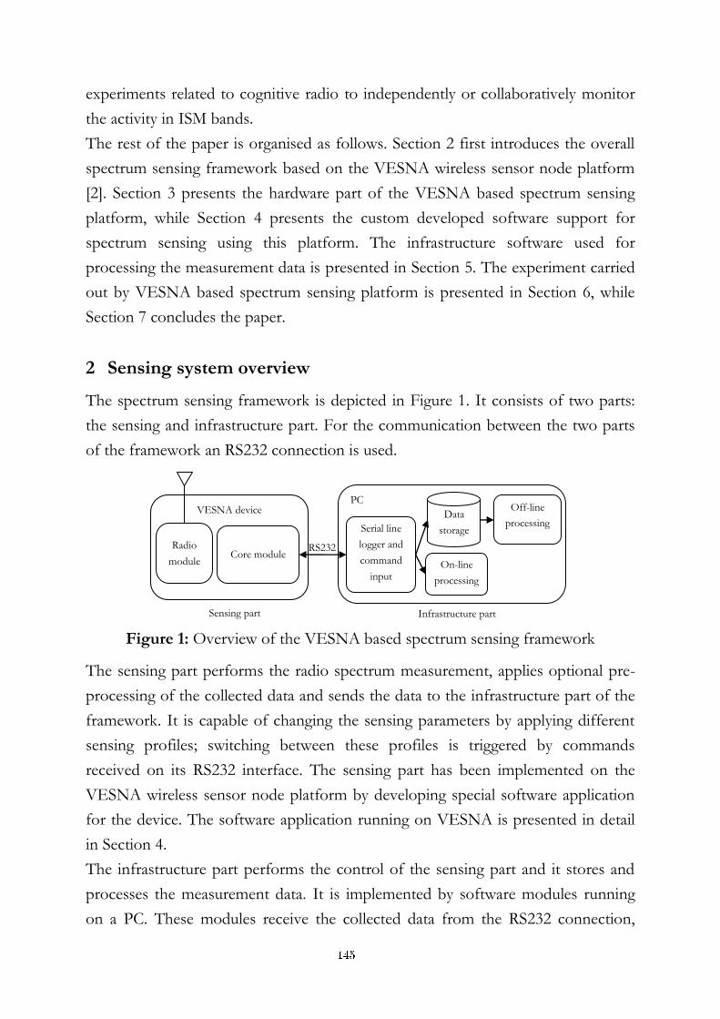
experiments related to cognitive radio to independently or collaboratively monitor
the activity in ISM bands.
The rest of the paper is organised as follows. Section 2 first introduces the overall
spectrum sensing framework based on the VESNA wireless sensor node platform
[2]. Section 3 presents the hardware part of the VESNA based spectrum sensing
platform, while Section 4 presents the custom developed software support for
spectrum sensing using this platform. The infrastructure software used for
processing the measurement data is presented in Section 5. The experiment carried
out by VESNA based spectrum sensing platform is presented in Section 6, while
Section 7 concludes the paper.
2 Sensing system overview
The spectrum sensing framework is depicted in Figure 1. It consists of two parts:
the sensing and infrastructure part. For the communication between the two parts
of the framework an RS232 connection is used.
Figure 1: Overview of the VESNA based spectrum sensing framework
The sensing part performs the radio spectrum measurement, applies optional pre-
processing of the collected data and sends the data to the infrastructure part of the
framework. It is capable of changing the sensing parameters by applying different
sensing profiles; switching between these profiles is triggered by commands
received on its RS232 interface. The sensing part has been implemented on the
VESNA wireless sensor node platform by developing special software application
for the device. The software application running on VESNA is presented in detail
in Section 4.
The infrastructure part performs the control of the sensing part and it stores and
processes the measurement data. It is implemented by software modules running
on a PC. These modules receive the collected data from the RS232 connection,
VESNA device
Radio
module
Core module
PC
Data
storage Serial line
logger and
command
input On-line
processing
Off-line
processing
Sensing part Infrastructure part
RS232
145
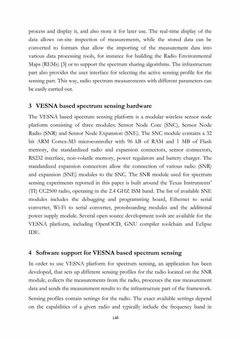
process and display it, and also store it for later use. The real-time display of the
data allows on-site inspection of measurements, while the stored data can be
converted to formats that allow the importing of the measurement data into
various data processing tools, for instance for building the Radio Environmental
Maps (REMs) [3] or to support the spectrum sharing algorithms. The infrastructure
part also provides the user interface for selecting the active sensing profile for the
sensing part. This way, radio spectrum measurements with different parameters can
be easily carried out.
3 VESNA based spectrum sensing hardware
The VESNA based spectrum sensing platform is a modular wireless sensor node
platform consisting of three modules: Sensor Node Core (SNC), Sensor Node
Radio (SNR) and Sensor Node Expansion (SNE). The SNC module contains a 32
bit ARM Cortex-M3 microcontroller with 96 kB of RAM and 1 MB of Flash
memory, the standardized radio and expansion connectors, sensor connectors,
RS232 interface, non-volatile memory, power regulators and battery charger. The
standardized expansion connectors allow the connection of various radio (SNR)
and expansion (SNE) modules to the SNC. The SNR module used for spectrum
sensing experiments reported in this paper is built around the Texas Instruments’
(TI) CC2500 radio, operating in the 2.4 GHZ ISM band. The list of available SNE
modules includes the debugging and programming board, Ethernet to serial
converter, Wi-Fi to serial converter, protoboarding modules and the additional
power supply module. Several open source development tools are available for the
VESNA platform, including OpenOCD, GNU compiler toolchain and Eclipse
IDE.
4 Software support for VESNA based spectrum sensing
In order to use VESNA platform for spectrum sensing, an application has been
developed, that sets up different sensing profiles for the radio located on the SNR
module, collects the measurements from the radio, processes the raw measurement
data and sends the measurement results to the infrastructure part of the framework.
Sensing profiles contain settings for the radio. The exact available settings depend
on the capabilities of a given radio and typically include the frequency band in
146
which the sensing should be performed, the channel bandwidth on which the radio
should operate, the list of frequencies on which the sensing band should be applied
and the number of samples that should be averaged in order to obtain one data
point. By using different sensing profiles, trade-offs can be made between the
parameters of the sensing, such as resolution, accuracy, bandwidth, speed of
sensing and minimal signal level than can be detected. The selection of sensing
profiles is controlled by the infrastructure part of the sensing framework, by
sending commands to the sensing part. These commands are received on the
RS232 interface on the SNC, and processed in software.
The data sent to the infrastructure is organized in lines; each line describes the
power level detected at each of the frequencies specified in the active sensing
profile. Besides measurement data, lines contain a timestamp of the measurement
and markers for line start and line end used for corruption detection at the end of a
sensing activity. If sensing is interrupted, the successfully transmitted lines can be
easily recovered based on the line start and line end markers.
5 Infrastructure software
The infrastructure part of the framework (i) allows the user to select the active
sensing profile, (ii) displays the spectrum measurement data in real time, in order to
allow the monitoring of the measurements and (iii) stores the spectrum data on the
PC, in order to allow off-line processing.
The selection of the current sensing profile is performed by manually typing the
command that selects a given sensing profile. The list of available sensing profiles
and a short description is provided by a “help” command. The real-time data
monitoring interface is shown in Figure 3. It presents the received signal power
versus time, in the frequency band defined by the active sensing profile. The same
data is saved on the PC, in order to be processed offline. The format of the saved
data is identical to the data transmitted on the RS232 connection; however, it is
guaranteed that the saved data contains only valid lines. In order to import the data
into MATLAB or Octave, scripts have been developed, which load the saved files
and stores the available data in data structures specific to the programs mentioned.
After this importing procedure, the data can be freely processed.
147
6 Experiments
The spectrum sensing framework presented in this paper has been used to analyse
the radio spectrum usage in the 2.4 GHz ISM band. Figure 3 presents the
measurement results obtained by the real-time data analyser. The frequency bands
used by Wi-Fi (2400–2483 MHz) have been scanned for several minutes. The
vertical lines on the plot are the result of a known limitation of the CC2500 radio.
The patterns appearing on the left side of the plot indicate the Wi-Fi activity. Based
on the plot, it can be concluded that the Wi-Fi devices have been transmitting on
the center frequency of 2412 MHz, which corresponds to the Wi-Fi channel 1.
Also, a weak signal can be observed around 2431 MHz.
Figure 2: Real-time data monitoring interface for the system
7 Applications and future work
A VESNA platform based spectrum sensing framework has been presented which
is capable of collecting information about radio spectrum usage. This information
could be used in optimization of radio networks, implementation of dynamic
spectrum access or as a sensing component for cognitive radio systems. The future
direction of this work is to integrate multiple sensing devices into one network, and
perform collaborative spectrum sensing and thus provide more comprehensive
measurements.
References:
[1] J. Mitola III and G. Q. Maguire, Jr., Cognitive radio: making software radios more personal, IEEE Personal Communications Magazine, vol. 6, nr. 4, pp. 13-18, Aug. 1999
[2] VESNA hardware platform. SensorLab. http://sensorlab.ijs.si/hardware.html
[3] Atanasovski, V., et. al.. Constructing radio environment maps with heterogeneous spectrum sensors. 2011 IEEE Symposium on New Frontiers in Dynamic Spectrum Access Networks (DySPAN), pp. 660-661, 3-6 May 2011
148

For wider interest
All radio systems, including mobile phone network, Wi-Fi for computer networks,
FM radio, satellite systems, use the same shared resource for communication: the
radio spectrum. This spectrum is managed by regulatory agencies, which allocate
frequency bands to various systems. A notable category of allocated frequency
bands are the Industrial, Scientific and Medical (ISM) bands, which can be freely
used for communication by any device. For example Wi-Fi and Bluetooth systems
use this band. In order to develop new technologies that operate in different
frequency bands, or to optimise existing systems, it is necessary to monitor the
radio activity in a given band.
A low-cost spectrum sensing framework has been developed, which is able to
monitor the signal power in the ISM frequency bands. This system is based on the
VESNA wireless sensor platform. Wireless sensor networks are usually low-power
networks of devices which collect information about their environment, such as
temperature, humidity, pressure. In this case the wireless sensor node hardware has
been used for collecting information about radio spectrum usage. This framework
is being used for collecting experimental data about new, experimental radio
systems, which will be more efficient. It is also planned to integrate the sensing
capabilities of this framework with more advanced radio systems.
149
Improving Performance of Wireless Mesh Networks with
Network Coding
Erik Pertovt1,2, Kemal Alič1,2, Aleš Švigelj1,2, Mihael Mohorčič1,2
1 Department of Communication Systems, Jožef Stefan Institute, Ljubljana, Slovenia
2 Jožef Stefan International Postgraduate School, Ljubljana, Slovenia
Abstract. In Wireless Mesh Networks, various mechanisms are used to
enhance the performance of the network. Network Coding (NC) is a novel
approach for enhancing the network performance as it can significantly
increases the network capacity through broadcasting encoded packets while
maintaining the desired Quality of Service. The effects of NC can be even
better exploited with appropriate support of NC-aware routing algorithms. In
this paper, we present implemented NC algorithms, routing supported
algorithms for NC, and custom designed NC simulation model that allows in
depth study of procedure effects, evaluation and comparison, eventually
leading into better understanding of the problem challenges and its
improvements. The results show that networks with NC included can handle
up to two times more traffic than existing networks where NC is not used.
Keywords: Network coding, coding-aware routing, simulation model.
1 Introduction
Wireless Mesh Networks (WMNs) are typical representatives of wireless access
networks, where nodes are connected to each other through multi-hop wireless
links. In WMNs, several mechanisms can be used to improve the network
performance, such as advanced physical layer techniques (e.g. multi-radio and
multi-channel technology), multi-path routing for load balancing and fault
tolerance, protocols for reliable data transport as for real-time delivery, protocols
for network management (i. e. mobility and power management, and network
monitoring), cross-layer design, scheduling algorithms, etc. The mechanism, which
experiences an increasing attention in the past few years in both, wired and wireless
150
networks, is network coding (NC), mainly due to promising results from the initial
research and testbed deployments.
NC enables encoding multiple packets either from the same or from different
traffic flows into one encoded packet for saving bandwidth and thus increasing the
network capacity while maintaining the desired Quality of Service parameters. In
wireless networks, NC exploits the broadcast nature of the wireless medium, where
nodes can overhear packets which are not destined to them, resulting in new
coding opportunities. These packets are later on needed for decoding process.
In our opinion, the true potential of NC in the network layer can only be used in
strong collaboration with routing, which has to be adopted to fully exploit NC
principles. By applying NC-aware routing [1], paths with more coding opportunities
can be discovered resulting in modified paths where more packets are being coded
together, thus using less bandwidth for transferring the same amount of traffic
from source to destination.
In order to design NC-aware routing algorithms, the understanding of NC and its
influences on other OSI layers has to be acquired, potentially allowing also cross
layer optimization. In this respect, simulation models present an appealing solution
for studying causes and consequences, as well as to evaluate and compare the
performance of different approaches. We have developed a NC simulation model
[2], using the OPNET Modeler [3] simulation tool. Several routing techniques, e.g.
Dijkstra’s, Bellman-Ford, and genetic ants-based routing algorithms and several
routing metrics, such as number of hops, distance, expected transmission count
(ETX), modified ETX, and coding enhanced ETX are being under investigation
[4]. In addition, we are examining the possibilities to improve metrics based on the
response of routing to the number of coding opportunities, packets queue lengths,
etc. Moreover, we are also developing new NC algorithms and NC-aware routing
procedures to better exploit NC principles.
NC simulation model currently supports our own routing-independent method
BON - Bearing opportunistic network coding [5], and the well-known COPE [6]
method. The results show that both BON and COPE significantly improve the
151
network performance in terms of network capacity as compared to reference
scenario (i.e. no-NC) cases where NC algorithms are not used.
In the rest of the paper, we describe the simulation model and present
implemented NC and routing algorithms. Furthermore, we show results comparing
COPE and BON methods, and the no-NC case.
2 Simulation Model
The architecture of the simulation model enables building networks with different
topology and parameter scenarios with little manual work. In such networks, NC
and NC-aware routing algorithms can be tested and evaluated.
2.1 Network Coding Simulation Model
The simulation model consists of several parts. The supporting network topology
generator is developed in MATLAB and is able to generate random wireless
topologies built around the arbitrary number of nodes that can communicate with
arbitrary number of neighbours through wireless links (graphically presented with
dashed lines in Figure 1) selected according to nodes positions and transmission
“range” or other parameters of nodes. The network description program, also
developed in MATLAB, prepares the information of desired topology, nodes, links
and parameters for communication procedures (e.g. throughputs, number of packet
retransmissions, loads, etc.) to import into the OPNET Modeler simulation model
[3], where the main simulation takes place. The latter consists of five functional
layers: (i) traffic generator is responsible for creating the network load, (ii) routing
module takes care of routing the packets through the network, (iii) the wireless
module takes care of successful packet distribution through the wireless channel to
the right address taking into account links conditions, (iv) network topology
module defines network architecture and links conditions, (v) network coding
module enables coding.
2.2 Implemented NC and Routing Algorithms
Two NC algorithms have already been implemented in the model. The first one is
an efficient and routing-independent method BON [5]. It is a novel method, which
152
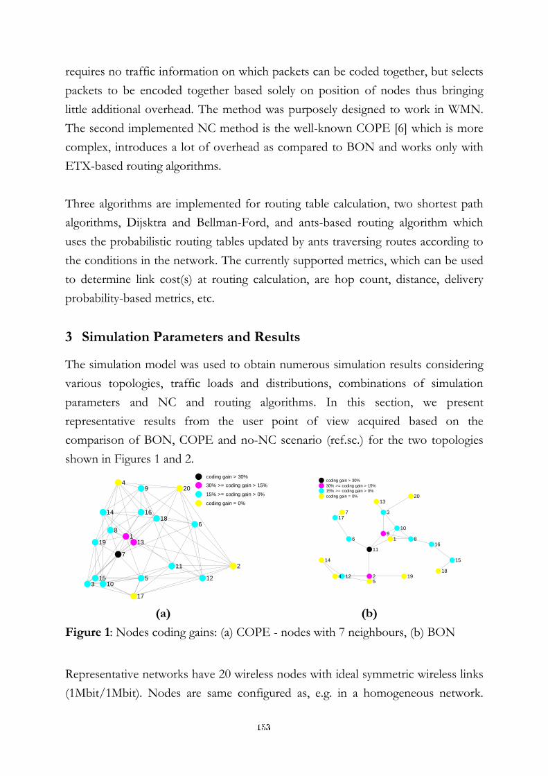
requires no traffic information on which packets can be coded together, but selects
packets to be encoded together based solely on position of nodes thus bringing
little additional overhead. The method was purposely designed to work in WMN.
The second implemented NC method is the well-known COPE [6] which is more
complex, introduces a lot of overhead as compared to BON and works only with
ETX-based routing algorithms.
Three algorithms are implemented for routing table calculation, two shortest path
algorithms, Dijsktra and Bellman-Ford, and ants-based routing algorithm which
uses the probabilistic routing tables updated by ants traversing routes according to
the conditions in the network. The currently supported metrics, which can be used
to determine link cost(s) at routing calculation, are hop count, distance, delivery
probability-based metrics, etc.
3 Simulation Parameters and Results
The simulation model was used to obtain numerous simulation results considering
various topologies, traffic loads and distributions, combinations of simulation
parameters and NC and routing algorithms. In this section, we present
representative results from the user point of view acquired based on the
comparison of BON, COPE and no-NC scenario (ref.sc.) for the two topologies
shown in Figures 1 and 2.
1
2
3
4
5
6
7
8
9
10
11
12
13
14
15
16
17
18
19
20
coding gain > 30%
30% >= coding gain > 15%
15% >= coding gain > 0%
coding gain = 0%
1
2
3
45
6
7
89
10
11
12
13
14 15
16
17
1819
20
coding gain > 30%
30% >= coding gain > 15%
15% >= coding gain > 0%
coding gain = 0%
(a) (b)
Figure 1: Nodes coding gains: (a) COPE - nodes with 7 neighbours, (b) BON
Representative networks have 20 wireless nodes with ideal symmetric wireless links
(1Mbit/1Mbit). Nodes are same configured as, e.g. in a homogeneous network.
153
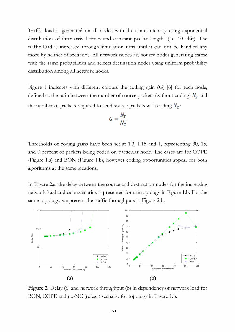
Traffic load is generated on all nodes with the same intensity using exponential
distribution of inter-arrival times and constant packet lengths (i.e. 10 kbit). The
traffic load is increased through simulation runs until it can not be handled any
more by neither of scenarios. All network nodes are source nodes generating traffic
with the same probabilities and selects destination nodes using uniform probability
distribution among all network nodes.
Figure 1 indicates with different colours the coding gain (G) [6] for each node,
defined as the ratio between the number of source packets (without coding) and
the number of packets required to send source packets with coding :
Thresholds of coding gains have been set at 1.3, 1.15 and 1, representing 30, 15,
and 0 percent of packets being coded on particular node. The cases are for COPE
(Figure 1.a) and BON (Figure 1.b), however coding opportunities appear for both
algorithms at the same locations.
In Figure 2.a, the delay between the source and destination nodes for the increasing
network load and case scenarios is presented for the topology in Figure 1.b. For the
same topology, we present the traffic throughputs in Figure 2.b.
0 20 40 60 80 100 120
10
100
1000
Network Load (Mbits/s)
Dela
y (
ms)
ref.sc.
COPE
BON
0 20 40 60 80 100 1200
10
20
30
40
50
60
70
80
90
100
Network Load (Mbits/s)
Netw
ork
Thro
ughput
(Mbits/s
)
ref.sc.
COPE
BON
(a) (b)
Figure 2: Delay (a) and network throughput (b) in dependency of network load for
BON, COPE and no-NC (ref.sc.) scenario for topology in Figure 1.b.
154
From the results, we can see that COPE can handle the highest given load, though
the BON method is not far behind, while the no-NC scenario can handle the
lowest load showing that BON and COPE significantly improve the network
capacity.
COPE only works on networks that use routing based on delivery probability
metric and is more demanding in terms of processing power and storage, since it
needs the information on the packets held by the neighbouring nodes.
Furthermore, it has high overhead, since nodes send out reports on the packets
they have acquired, thus additionally loading the network in its normal operational
conditions. BON, on the other hand, is an efficient method that is not related to
any routing protocol. It needs less processing power and storage capacity than
COPE and introduces less overhead.
4 Conclusion and Further Work
In this paper, we present an overview of our work in NC with representative results
showing that NC supported WMN networks significantly improve the network
capacity. The results were obtained through briefly presented custom-designed NC
simulation model. Our future work is focusing on further investigation of new NC
algorithms and NC-aware routing.
References:
[1] M. A. Iqbal, B. Dai, B. Huang, A. Hassan, S. Yu, "Survey of network coding-aware routing protocols in wireless networks," in Journal of Network and Computer Applications, vol.34, no. 6, pp. 1956-1970, August 2011.
[2] K. Alič, E. Pertovt, A. Švigelj, "Simulation environment for network coding," in Mosharaka International Conference on Communications, Networking and Information Technology (MICCNIT 2011), Dubai, UAE, 2011.
[3] OPNET web page, available at http://www.opnet.com/, accessed May 2010.
[4] E. Pertovt, K. Alič, M. Mohorčič, A. Švigelj, "ETX-based Metrics and Adapted Routing Algorithms for Network Coding," in 20th Electrotechnical and Computer Science Conference (ERK 2011), Portorož, Slovenija, September 2011.
[5] K. Alič, E. Pertovt, A. Švigelj, ‘unpublished’ "Routing-Independent Practical Network Coding Algorithm," 2012 International Symposium on Network Coding (NetCod 2012), Boston, MA, USA, June 2012.
[6] S. Katti, H. Rahul, W. Hu, D. Katabi, M. Médard, and J. Crowcroft, "XORs in the Air: Practical Wireless Network Coding," IEEE/ACM Transactions on networking, vol. 16, June 2008.
155

For wider interest
Wireless Mesh Networks (WMN):
- typical representatives of wireless access networks, where nodes, such as wireless
routers, are highly connected to each other through multi-hop wireless links
enabling various large-scale communications as e.g. Internet connection
Network Coding (NC):
- enables encoding multiple packets either from the same or from different traffic
flows into one encoded packet for saving bandwidth and thus increasing the
network throughput while maintaining the desired Quality of Service
Network simulation model for network coding:
- supports building WMN networks
- support for different NC and routing algorithms
Our work:
- studying, evaluating and comparing causes and consequences on the network
performance of different NC approaches
- investigating several routing techniques for NC
- improving metrics based on the response of routing to the number of coding
opportunities, packets queue lengths, etc.
- developing new NC and NC-aware routing algorithms and protocols for different
environments
Results:
- NC significantly improves the performance of WMN; network throughput is
increased and end-to-end packet delay is decreased
Our goal:
- further improvement of the capacity of WMN and similar networks through
novel NC and routing techniques
156
Mobile terminal as opportunistic sensor network device for
research on cognitive radio networks
Marko Pesko1,3, Luka Vidmar1, Mitja Štular1, Mihael Mohorčič2,3
1 Telekom Slovenije, Cigaletova 15, 1000 Ljubljana, Slovenia
2 Department of Communication Systems, Jožef Stefan Institute, Ljubljana, Slovenia
3 Jožef Stefan International Postgraduate School, Ljubljana, Slovenia
Abstract. The cognitive radio (CR) concept is promising to relax the pressure
on the available radio resources and increase the efficiency of their use by
dynamic spectrum allocation and spectrum sharing. Research focus related to
CR networks is recently moving from simulation-based investigations to actual
testbeds, many of them based on Wireless Sensor Networks (WSN), which
support some CR research scenarios. Advanced mobile terminals can extend
WSN features with mobility, sensing and measurements collection. This paper
presents the concept of using a mobile terminal as an opportunistic sensor
network device, capable of cooperation with dedicated sensor nodes to build
Radio Environment Map to support the operation of CR networks.
Keywords: Mobile terminals, sensor nodes, Wireless Sensor Networks
opportunistic, spectrum sensing, cognitive radio, hidden node.
1 Introduction
There are various wireless devices around us, which share the same frequency
spectrum. In this respect, national and regional regulators recommend, set, and
enforce output power and energy radiation rules for spectrum frequencies divided
to the licenced and non-licenced bands. Due to such regulation, frequency bands
are not fully exploited neither in time nor space. To solve this issue, the cognitive
radio (CR) concept was introduced [1]. Its main advantage in comparison to
traditional radios used today is a cognition cycle, which includes radio environment
observation, learning from previous experiences and planning its own operation.
While majority of initial CR related research relied on computer simulations, more
recent studies started to investigate spectrum sensing, opportunistic spectrum
157
access and spectrum sharing procedures in real testbeds, many of them based on
Wireless Sensor Networks (WSN). Practical experimentations in this field can be
performed in ISM (Industrial Scientific Medical) frequency bands, in which
expensive professional measurement equipment (e.g. spectrum analysers), medium-
cost devices (e.g. USRPs) as well as low-cost devices, such as WSN nodes, can be
used for testing. However, real sensing scenarios’ goal is to have a maximum
number of measuring devices available in order to acquire the most accurate results
in the specific field of interest. To achieve this, sensor nodes seem a suitable choice,
since they offer a good compromise between the price, the number of devices, and
their computing, communication and sensing capabilities. As presented in [2], there
are already several WSN testbeds, which use dedicated WSN gateway(s) to transfer
the sensor measurements to the remote server locations for further analysis and
processing. However, static deployment of dedicated sensor nodes and gateways is
not always an optimal solution, resulting in many initiatives to use advanced mobile
terminals equipped with different embedded sensors and communication interfaces
as opportunistic sensors nodes and/or gateways [3]. In this respect, the aim of this
paper is to present the mobile terminals’ sensing capability and opportunistic
sensor network role in CR research scenario. In the following, Section 2 presents
mobile terminals’ sensing and communication features. Section 3 presents
difficulties and solutions of accessing sensors on the mobile terminals. Section 4
depicts our considered spectrum sensing scenario and in parallel presents a possible
solution for the issues from Section 3. Finally, Section 5 concludes the paper.
2 Sensing and communication features of mobile terminals
Mobile terminals can be treated as a specific type of sensor nodes, however, their
embedded higher processing, storing and communicating capabilities reflect in
larger energy consumption, mostly due to the high resolution displays and relatively
fast communication interfaces. It can be noticed that also low-power WSN adopted
radios, in addition to Bluetooth technology, are slowly gaining the attention of the
mobile terminals developers, whereas they already integrate many different types of
sensors.
158

Table 1 Android most common supported embedded and virtual sensors
Microphone Magnetic field sensor Pressure sensor
Camera Gravity sensor Proximity sensor
Touch screen display Gyroscope sensor Relative humidity sensor
Buttons Light sensor Rotation vector sensor
Global Positioning
Sensor (GPS) Ambient temperature sensor Linear accelerometer sensor
Orientation sensor Radio interfaces sensors for
GSM, CDMA (logical level)
Radio interfaces sensors for
Wi-Fi, Bluetooth (logical level)
Several most common embedded and virtual sensors, supported by increasingly
popular Android-based mobile terminals, are listed in Table 1, however, none of
them is actually appropriate for spectrum sensing on the physical level. A solution
could be implemented through the usage of additional external sensors. Wired
connections with sensors can be established over the serial connectors, USB
connectors or even SD and uSD card sockets, while wireless connections are
mostly available over high-power consuming Wi-Fi, medium-power Bluetooth or
low-power WSN communication interfaces, if available.
3 Challenges related to mobile terminals used as sensor nodes
To efficiently access and retrieve sensor measurements from dedicated sensor
nodes and opportunistic sensor network devices (e.g. mobile terminals) in the
public networks, both device types must communicate and cooperate. However,
access to mobile terminals through the internet over the mobile network cannot be
done in a straightforward manner. In principle, mobile terminals can only post
sensor measurements over self-created data session called Packet Data Protocol
(PDP) context in GSM/UMTS and EPS bearer in LTE to the servers in the public
networks, as depicted in Figure 1. Namely, all measurement retrieval requests
coming in the opposite direction, as depicted by the red line in Figure 1, are not
possible, since the mobile operators normally block all communication session
initiation attempts coming from the public networks.
159

...
WSN
WSN
WSN
WSN
WSN BSCsRNCs
CBC TM IDS/IPS FW
Users security policy
SGSN /MME GGSNs /PGW
ROUTER INTERNET
SERVER 1
SERVER N
USERS
SERVER 2
Figure 1: Typical sensor measurements transport routes over the mobile network
4 Spectrum sensing scenario with opportunistic sensor devices
Our considered sensing scenario for practical demonstration of Radio
Environment Map (REM) [4] creation is depicted in the left side in Figure 2. It
consists of the fixed sensor nodes (F) forming WSN and mobile opportunistic
sensor network device(s) (M). This enables spectrum sensing over the specific area
of interest to build an efficient REM needed for detection of the hidden node or
primary user transmitter (H), as presented on the right side in Figure 2.
Such scenario can be realized with majority of the mobile terminals available
despite the issues presented in Section 3. On the mobile network side a private
access point name (APN) for a connection with its own security policy has to be
prepared to allow the access to measurements from the external networks, as
depicted in Figure 1 with the green line. To prove the concept for the mobile
terminal, we took Android-based Samsung I9100 mobile terminal, which lacks
WSN compatible radios and sensors being capable of spectrum sensing. We
selected VESNA sensor node [5] capable of spectrum sensing to which we
connected Roving Networks XBT RN-41 Bluetooth module. Thus, we enabled
communication among mobile terminal and VESNA node together presenting an
F
F F
F
M
F
REMspectrum sensing
H
Figure 2: Spectrum sensing scenario with sensor nodes and opportunistic sensor
network device capable to cooperate and construct REM
160
opportunistic sensor network device. A test software for managing such a virtual
sensor network device was written as a code in C programming language on the
side of VESNA node and as Java-based Android application communicating with
data frames, presented in [6].
5 Conclusion and future work
In this paper we outlined mobile terminals’ sensing capabilities and their prospects
to become opportunistic sensor network devices capable of cooperating with
WSNs in spectrum sensing scenarios if complemented by appropriate sensors.
Their sensor measurements can be accessed over the mobile network over private
APNs. Our further work includes testing of opportunistic sensor network devices
in real outdoor scenarios with the aim to support development of algorithms for
hidden node detection.
Acknowledgements
This work has been in part funded by the European Community from the
European Social Fund under the Operational Programme Human Resources
Development for the period 2007 – 2013.
References
[1] J. Mitola III and G. Maguire, "Cognitive radio: making software radios more
personal," IEEE Personal Communications, vol. 6, pp. 13-18, 1999.
[2] M. Vučnik, C. Fortuna, M. Porcius, and M. Mohorčič, "WSN Testbeds For Lighting
Control And Environmental Monitoring," in 3rd Jožef Stefan International
Postgraduate School Students Conference, Ljubljana, Slovenia, 2011.
[3] M. Shin, C. Cornelius, D. Peebles, A. Kapadia, and D. Kotz, "AnonySense: A system
for anonymous opportunistic sensing," Pervasive and Mobile Computing, vol. 7, 2011.
[4] V. Atanasovski, J. v. d. Beeky, A. Dejonghe, D. Denkovski, L. Gavrilovska, S.
Grimoudyy, P. Mähönen, M. Pavloski, V. Rakovic, J. Riihijärvi, and B. Sayracyy,
"Constructing Radio Environment Maps with Heterogeneous Spectrum Sensors," in
IEEE International Symposium on Dynamic Spectrum Access Networks, Aachen,
Germany, 2011.
[5] VESNA hardware platform. Available: SensorLab http://sensorlab.ijs.si/hardware.html
[6] M. Pesko, M. Štular, M. Vučnik, M. Smolnikar, and M. Mohorčič, "Bluetooth-based
mobile gateway for wireless sensor network," in The Second International Workshop
on Sensing Technologies in Agriculture, Forestry and Environment, Belgrade, Serbia
2011.
161

For wider interest
Wireless Sensor Networks (WSN):
- are wireless networks build of spatially distributed small and low-power
autonomous devices called sensor nodes, equipped with heterogeneous sensors to
measure various physical phenomena over specific area of interest.
Opportunistic sensor network devices:
- are devices which can be used as sensor nodes,
- can be mobile terminals which can opportunistically cooperate with WSNs in
various scenarios.
Cognitive radio principles:
- include methods for more efficient spectrum usage,
- enable multiple users sharing the same frequency spectrum in a cooperative or
competitive way,
- enable non-licensed secondary users to communicate on the same frequencies as
licenced primary users if and only if they do not cause any harmful interference.
Hidden node problem:
- is a problem in cognitive networks where secondary users in some situations are
not aware of the primary user’s presence in the vicinity.
Our work:
- outlining mobile terminals’ features which enable them becoming opportunistic
sensor network devices,
- pointing out mobile network issues related to sensor measurements access on
mobile terminals and their lack of WSN compatible communication interfaces,
- presenting solutions for these issues.
Future work:
- to test mobile terminals as opportunistic sensor network devices in real testbeds
meant for spectrum sensing and efficient Radio Environment Maps building to
support multiple issues in cognitive networks.
162
Inteligentni sistem za zaznavanje zdravstvenih težav pri starejših
Bogdan Pogorelc1,2,3
1 Institut »Jožef Stefan«, Odsek za inteligentne sisteme, Ljubljana, Slovenija
2 Špica International d.o.o., Ljubljana, Slovenija
3 Mednarodna podiplomska šola Jožefa Stefana, Ljubljana, Slovenija
Povzetek. Članek predlaga semantični in splošni pristop k prepoznavanju
zdravstvenih težav starejših. Gibanje oseb je zajeto s sistemom za zajem
gibanja in izhodne časovne vrste koordinat so modelirane z obema
predlaganima pristopoma. Semantični pristop uporablja atribute na osnovi
medicinskega znanja (semantične atribute) in klasifikacijsko metodo podpornih
vektorjev. Splošni pristop ima za atribute vse izmerljive kote sklepov in
klasificira s kombinacijo algoritma k-najbližjih sosedov in modifikacijo
algoritma dinamičnega ukrivljanja časa (DTW). Kljub temu da je drugi pristop
splošnejši in uporaben tudi za druge klasifikacijske metode, doseže primerljivo
visoko klasifikacijsko točnost kot semantični pristop.
Ključne besede Zdravstvene težave, hoja, podatkovno rudarjenje, dinamično
ukrivljanje časa.
1 Uvod
Razvite države se soočajo s hitro rastjo svojega prebivalstva. Napovedi kažejo, da
naj bi se odstotek populacije nad 65 let v razvitih državah povečal iz 7,5 % v 2009
na 16 % v 2050 [1]. Starejši navadno živijo izolirani od potomcev, zato v primeru
bolezni težko dobijo pravočasno pomoč. Namen te študije je razviti tehnologije, ki
bi olajšale njihovo samostojno življenje.
Dva pristopa podatkovnega rudarjenja k inteligentnemu in vseprisotnemu sistemu
nadzora zdravja z namenom razpoznati nekaj najpogostejših in najpomembnejših
bolezni starejših, ki so lahko razpoznane preko opazovanja in analize karakteristik
njihovega gibanja, sta predlagana v prispevku. Semantični pristop uporablja atribute
na osnovi medicinskega znanja (semantične atribute) in metodo podpornih
163
vektorjev. Splošni pristop ima za atribute vse izmerljive kote sklepov v kombinaciji
z algoritmom k-najbližjih sosedov in dinamičnega ukrivljanja časa (DTW). Naloga
je klasificirati vzorce hoje v pet različnih zdravstvenih stanj, eno zdravo in štiri
bolezenska.
S sistemom za zajem gibanja, ki sestoji iz značk, pritrjenih na telo in senzorjev,
nameščenih v stanovanju, je zajeto gibanje uporabnika. Izhodne časovne vrste
koordinat so obdelane s predlaganima pristopoma, da bi razpoznali specifično
zdravstveno težavo.
V literaturi je zajem gibanja navadno narejen z inercialnimi senzorji [2, 5], s
strojnim vidom, s specifičnim senzorjem za merjenje kota upognjenosti sklepa [3]
ali z elektromiografijo [4]. V naši študiji smo uporabili sistem (infrardečih) IR
senzorjev z značkami pritrjenimi na telo. Ne naslavljamo samo razpoznave
značilnih aktivnosti, kot je hoja, sedenje, ležanje, itd., kot je realizirano npr. v [6, 8],
ampak razpoznavamo tudi zdravstvene težave. Z uporabo podobnega sistema za
zajem podatkov so v [7] ločevali med hemiplegijo in diplegijo.
Pogostejši pristop iz sorodnega dela je zajem podatkov s sistemom za zajem gibanja
in kasnejša ročna analiza podatkov [3, 4, 9]. Tak pristop ima pomanjkljivost v
primerjavi z našim, da zahteva stalno pregledovanje strokovnjakov.
2 Materiali in metode
Zdravstvene težave za detekcijo. Vse zdravstvene težave, ki jih prepoznavamo,
so bile predlagane s strani sodelujočega medicinskega strokovnjaka, na osnovi
pogostosti nad 65 let starosti, medicinske pomembnosti in možnosti razpoznavanja
iz gibanja. Sistem hojo klasificira kot: hemiplegijo (navadno po možganski kapi),
Parkinsonovo bolezen, bolečino v nogi, bolečino v hrbtu in referenčno zdravo
hojo.
Atributi za podatkovno rudarjenje. Meritve sestavljajo pozicije koordinat v x,y,z
za 12 značk nošenih na ramenih, komolcih, zapestjih, kolkih, kolenih in gležnjih,
zajete s sistemom za zajem gibanja Smart z 10 Hz. Primeren prikaz uporabnikovega
gibanja je bil pomemben del naše študije.
164
Semantični pristop smo zasnovali na osnovi dejstva, da zdravnik diagnosticira
obravnavane zdravstvene probleme iz opazovanja hoje [10]. Ker so si vzorci
podobni, mora biti pozoren na veliko detajlov, ki smo jih poskušali zapisati z
merljivimi spremenljivkami. Za nalogo avtomatske prepoznave bolezni smo
predlagali in testirali uporabo 13 značilk, kot npr. : povprečni kot komolcev, razlika
med maksimalno in minimalno višino ramena, razlika hitrosti gležnjev.
Pri splošnem pristopu je gibanje predstavljeno z enostavnimi in splošnimi atributi,
da bo klasifikator s temi atributi delal dobro tudi na drugačnih gibanjih, saj
zajamemo le majhen del vseh možnih gibanj. Upoštevajoč našteto smo zasnovali
atribute kot kote med sosednjimi deli telesa:
• kot levega in desnega ramena glede na zgornji del trupa v trenutku t:
• kot levega in desnega kolka glede na spodnji del trupa
• kot med spodnjim in zgornjim delom trupa:
• levi in desni komolčni ter levi in desni kolenski kot:
Koti med deli telesa, ki rotirajo v več kot eno smer, so izraženi s kvaternioni.
DTW. Dinamično ukrivljanje časa (DTW) poravna 2 časovni vrsti na način, da
minimizira neko mero. Optimalna poravnava je dobljena s preslikavo več
zaporednih vrednosti ene časovne vrste v eno vrednost druge časovne vrste in tako
je lahko DTW računan tudi na časovnih vrstah različnih dolžin. V nasprotju z
Evklidsko razdaljo, DTW lahko najde podobnosti med vzorcema dveh časovnih
vrst, tudi če ta vzorca nista časovno poravnana ali pa sta vzorca različnih dolžin.
Prispevek: multivariantno dinamično ukrivljanje časa. DTW algoritem, ki je
navadno opisan v literaturi, je uporabljen le za poravnavo univariantnih časovnih
vrst. Splošni pristop te študije pa poravnava multivariantne časovne vrste. Najprej
je vsaka točka zajete časovne vrste pretvorjena v prostor kotnih atributov, kjer bo
izvedena klasifikacija.
Imamo testno meritev, ki jo želimo poravnati z učno meritvijo (kjer je bil
klasifikator naučen) in najprej izračunamo matriko lokalnih razdalj d(i,j), v kateri
vsak element (i,j) predstavlja lokalno razdaljo med j-to časovno točko učne in i-to
časovno točko testne meritve. Naj bo Ljf element generičnega atributnega vektorja
glede na učno meritev in Tif naj bo element atributnega vektorja, relativno na novo
165
testno meritev za razpoznavo, kjer je 1<=f<=N upoštevani atribut. Za definicijo
lokalne razdalje je bila uporabljena Evklidska razdalja
Na osnovi matrike lokalnih razdalj je zgrajena matrika globalnih razdalj D. Končni
izhod algoritma je vrednost minimalne globalne razdalje za celotno poravnavo
DTW in je najdena v zadnji vrstici in stolpcu, D(Rl,Cl).
3 Eksperimenti in rezultati
Meritve so obsegale 256 posnetkov zdravih posameznikov in posameznikov z
določenimi zdravstvenimi težavami, pri čemer je bil vsak posameznik 4-5 krat
posnet z različnimi hitrostmi izvajanja aktivnosti.
Pri splošnem pristopu klasifikacijski proces upošteva eno vhodno testno časovno
vrsto, ki jo primerja z vsemi ostalimi, da najde minimalno globalno razdaljo za
vsako poravnavo in sklepa, da je vhodna meritev istega razreda kot učna meritev, ki
ima najmanjšo razdaljo do te vhodne meritve.
Evaluacija "izpusti-enega" je rezultirala v klasifikacijski točnosti 97,9 % oz. 97,6 %
za semantični oz. splošni pristop.
4 Zaključek
Prispevek predstavlja semantični in splošni pristop k detekciji zdravstvenih težav za
namen podaljšanja samostojnega življenja starejših. Metoda "izpusti-enega" da
klasifikacijski točnosti 97,9 % oz. 97,6 % za semantični oz. splošni pristop.
Semantični pristop je zahtevnejši za izvedbo zaradi gradnje specifičnih semantičnih
atributov, ki zahtevajo medicinsko znanje. Kljub temu, da je drugi pristop bolj
splošen in lahko razpozna tudi nove vrste gibanj, dosega visoke klasifikacijske
točnosti, podobne semantičnemu pristopu.
Zahvala
Operacije, ki so pripeljale do tega članka, je delno sofinancirala Evropska Unija,
Evropski socialni sklad. Avtor članka se zahvaljuje mentorju prof dr. Matjažu
Gamsu za pomoč.
166
Literatura:
[1] United Nations (2009) World Population Ageing. Report.
[2] Strle D., Kempe V., “MEMS-based inertial systems”, MIDEM 37(2007)4, 199-209.
[3] Ribarič S., Rozman J., “Sensors for measurement of tremor type joint movements”, MIDEM 37(2007)2, 98-104.
[4] Trontelj J., et al., “Safety margin at mammalian neuromuscular junction – an example of the significance of fine time measurements in neurobiology”, MIDEM 38(2008)3, 155- 160.
[5] Bourke A.K et al., An optimum accelerometer configuration and simple algorithm for accurately detecting falls. In Proc. BioMed 2006 (2006), 156–160.
[6] Confidence Project. http://www.confidence-eu.org.
[7] H. Lakany, Extracting a diagnostic gait signature. Patt. recognition 41(2008), 1627–1637.
[8] Luštrek, M., and Kaluža, B. Fall detection and activity recognition with machine learning. Informatica 33, 2 (2009).
[9] Moore ST, et al., Long-term monitoring of gait in Parkinson’s disease, Gait Posture (2006).
[10] Pogorelc B, Bosnic Z, Gams M (2012) Automatic recognition of gait-related health problems in the elderly using machine learning. Multimed Tools Appl 58:333–354. doi:10.1007/s11042-011-0786-1.
167

Za širši interes
V razvitem svetu je vedno večji delež starejšega prebivalstva. Starejši navadno živijo
izolirani od otrok, zato v primeru bolezni ali poškodbe težko dobijo pravočasno
pomoč. Namen te študije je razviti tehnologije, ki bi olajšale samostojno življenje
starejših. Članek predstavlja dva pristopa k razvoju sistema za detekcijo
zdravstvenih težav pri starejših z namenom podaljševanja njihovega samostojnega
življenja. Če je zaznana zdravstvena težava, sistem avtomatsko obvesti medicinsko
službo. Gibanje starejših je zajeto s sistemom za zajem gibanja in celoten sistem je
naučen, da prepoznava specifične zdravstvene težave. Semantični pristop uporablja
semantične atribute, ki jih uporablja zdravstvena stroka, splošni pa za atribute
uporablja vse izmerljive kote sklepov namesto specifičnih atributov za posamezne
bolezni. Kljub temu dobro prepoznava zdravstvene težave, podobno kot
semantični in pristopi iz literature.
168
Sentiment analysis on tweets in a financial domain
Jasmina Smailović1,2, Miha Grčar1, Martin Žnidaršič1
1 Dept of Knowledge Technologies, Jožef Stefan Institute, Ljubljana, Slovenia
2 Jožef Stefan International Postgraduate School, Ljubljana, Slovenia
Abstract. This paper investigates whether sentiment analysis of public mood
derived from large-scale Twitter feeds can be used to identify important events
and predict movements of stock prices. We used the volume and sentiment
polarity of Apple financial tweets to identify important events and predict
future movements of Apple stock prices. Statistical analysis using the Granger
causality test showed that we were able to predict the rise or fall in closing
price of Apple stocks two days before the change happens.
Keywords: sentiment analysis, classification, Twitter, stock price prediction.
1 Introduction
Sentiment analysis or opinion mining [1] is a research area aimed at detecting the
authors’ attitude, polarity (positive or negative) or opinion about a given topic
expressed in a document collection. In this paper we investigate whether sentiment
analysis of public mood, derived from large-scale collections of daily posts from
online microblogging service Twitter can predict movements of stock prices.
Specifically, we analyse Apple financial tweets to identify important events and
predict the movement of Apple stock prices.
Trying to determine the future revenue or stock value has been attracting great
attention of numerous researches. Early research on this topic claimed that stock
price movements do not follow any patterns or trends and past price movements
cannot be used to predict the future ones [2]. Later studies, however, show the
opposite [3][4]. Recent research indicates that the analysis of online texts such as
blogs, web pages and social networks can predict trends of various economic
phenomena. It was shown [5] that blog posts can be used to predict spikes in actual
169
consumer purchase decisions. Sentiment analysis of weblog data was used to
predict movie success [6]. Twitter posts were also shown to be useful when
predicting box-office revenues of movies in advance of their release [7].
Furthermore, it has been shown [8] that the stock market itself is a direct measure
of social mood. So, it is reasonable to expect that the analysis of public mood can
be used to predict movement of stock market values. Moreover, Bollen et al. [9]
show that changes in a specific public mood state can predict daily changes in the
closing values of the Dow Jones Industrial Average index.
The paper is structured as follows: selection of data preprocessing settings for the
SVM classifier is explained in Section 2, followed by an example in Section 3.
Conclusions are given in Section 4.
2 Selection of data preprocessing settings for the SVM classifier
Here we describe how the most appropriate classifier for sentiment analysis of
financial tweets was chosen. Three common approaches to sentiment analysis are:
machine learning, lexicon-based methods and linguistic analysis. In this work we
use the machine learning approach. In this approach, classification refers to a
procedure for assigning a given piece of input data (instance) into one of a given
number of categories (classes). In our case, input data is a tweet and it can be
classified into one of two categories: positive or negative, which represent attitude
of the tweet`s author. An instance is described by a vector of features (in our case,
words and word pairs), also called attributes, which constitute a description of all
known characteristics of the instance. An algorithm that implements classification
is known as a classifier. Classification usually refers to a supervised procedure, i.e., a
procedure that learns to classify new instances based on a model learnt from a
training set of instances that have been properly labelled. For our training set we
used a collection of 1,600,000 (800,000 positive and 800,000 negative) tweets
collected by the Stanford University [10], where positive and negative emoticons
were used as labels. For testing we used a set of manually labelled 177 negative and
182 positive tweets from the same source [10]. The SVMperf classifier [11] was used
for training and testing. It is an implementation of the Support Vector Machine
machine learning algorithm. As attribute weights, we used TFIDF (term frequency–
170
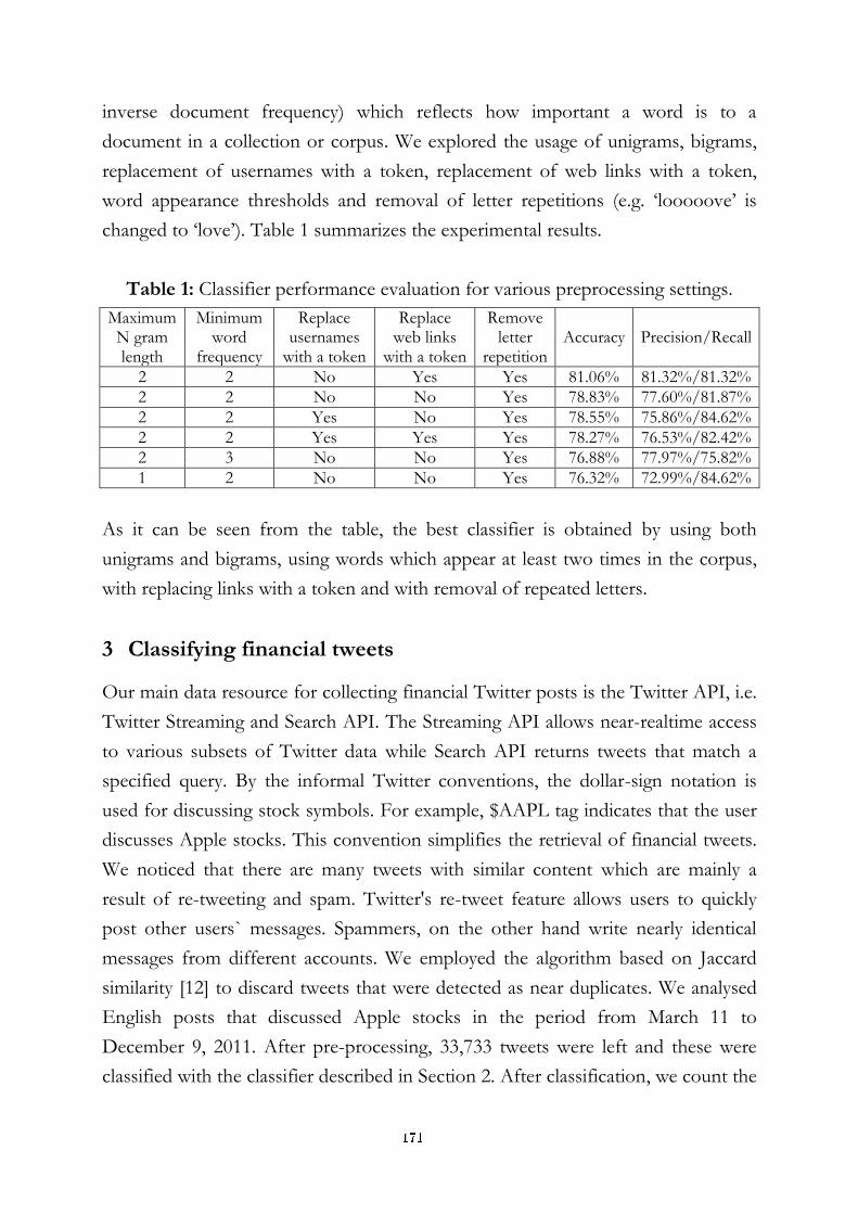
inverse document frequency) which reflects how important a word is to a
document in a collection or corpus. We explored the usage of unigrams, bigrams,
replacement of usernames with a token, replacement of web links with a token,
word appearance thresholds and removal of letter repetitions (e.g. ‘looooove’ is
changed to ‘love’). Table 1 summarizes the experimental results.
Table 1: Classifier performance evaluation for various preprocessing settings.
Maximum N gram length
Minimum word
frequency
Replace usernames
with a token
Replace web links
with a token
Remove letter
repetition Accuracy Precision/Recall
2 2 No Yes Yes 81.06% 81.32%/81.32%
2 2 No No Yes 78.83% 77.60%/81.87%
2 2 Yes No Yes 78.55% 75.86%/84.62%
2 2 Yes Yes Yes 78.27% 76.53%/82.42%
2 3 No No Yes 76.88% 77.97%/75.82%
1 2 No No Yes 76.32% 72.99%/84.62%
As it can be seen from the table, the best classifier is obtained by using both
unigrams and bigrams, using words which appear at least two times in the corpus,
with replacing links with a token and with removal of repeated letters.
3 Classifying financial tweets
Our main data resource for collecting financial Twitter posts is the Twitter API, i.e.
Twitter Streaming and Search API. The Streaming API allows near-realtime access
to various subsets of Twitter data while Search API returns tweets that match a
specified query. By the informal Twitter conventions, the dollar-sign notation is
used for discussing stock symbols. For example, $AAPL tag indicates that the user
discusses Apple stocks. This convention simplifies the retrieval of financial tweets.
We noticed that there are many tweets with similar content which are mainly a
result of re-tweeting and spam. Twitter's re-tweet feature allows users to quickly
post other users` messages. Spammers, on the other hand write nearly identical
messages from different accounts. We employed the algorithm based on Jaccard
similarity [12] to discard tweets that were detected as near duplicates. We analysed
English posts that discussed Apple stocks in the period from March 11 to
December 9, 2011. After pre-processing, 33,733 tweets were left and these were
classified with the classifier described in Section 2. After classification, we count the
171
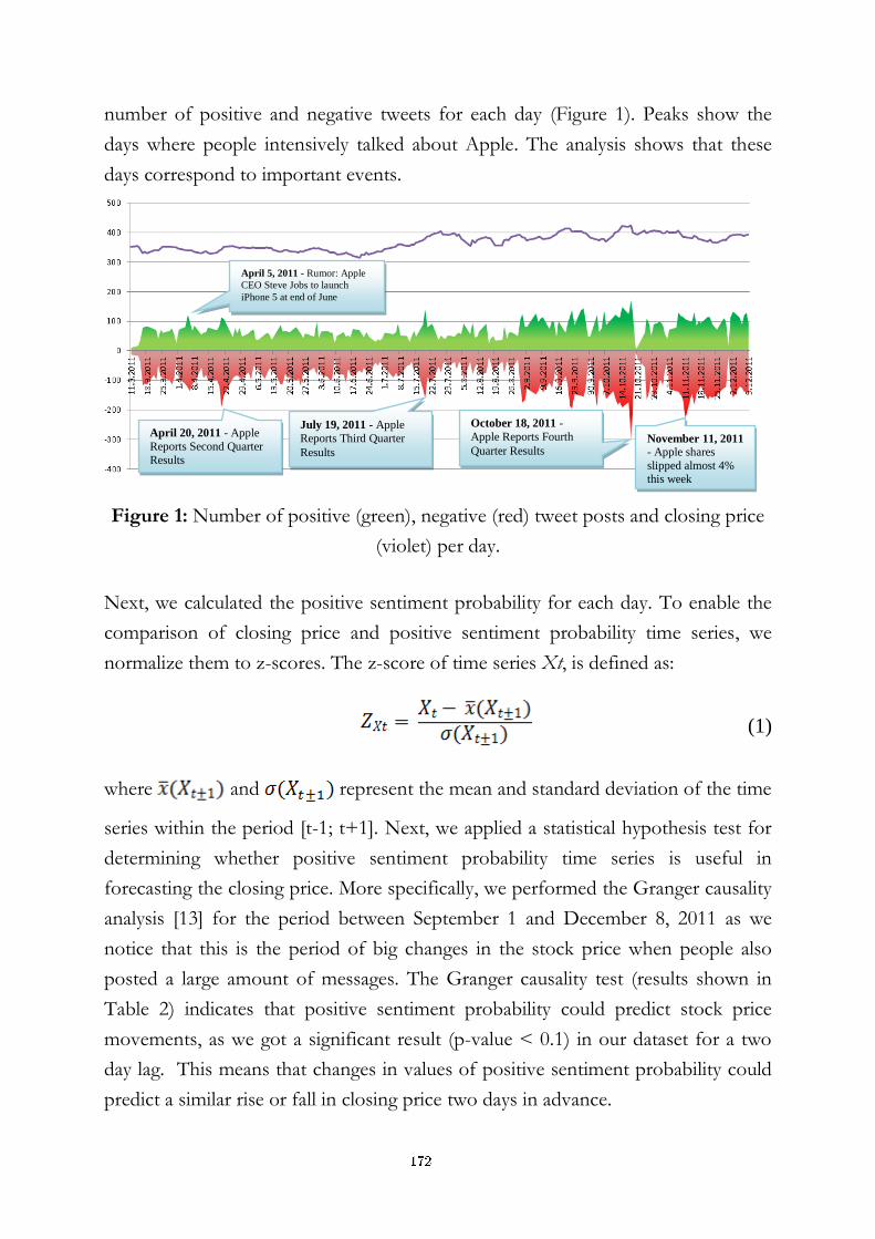
number of positive and negative tweets for each day (Figure 1). Peaks show the
days where people intensively talked about Apple. The analysis shows that these
days correspond to important events.
Figure 1: Number of positive (green), negative (red) tweet posts and closing price
(violet) per day.
Next, we calculated the positive sentiment probability for each day. To enable the
comparison of closing price and positive sentiment probability time series, we
normalize them to z-scores. The z-score of time series Xt, is defined as:
(1)
where and represent the mean and standard deviation of the time
series within the period [t-1; t+1]. Next, we applied a statistical hypothesis test for
determining whether positive sentiment probability time series is useful in
forecasting the closing price. More specifically, we performed the Granger causality
analysis [13] for the period between September 1 and December 8, 2011 as we
notice that this is the period of big changes in the stock price when people also
posted a large amount of messages. The Granger causality test (results shown in
Table 2) indicates that positive sentiment probability could predict stock price
movements, as we got a significant result (p-value < 0.1) in our dataset for a two
day lag. This means that changes in values of positive sentiment probability could
predict a similar rise or fall in closing price two days in advance.
April 20, 2011 - Apple
Reports Second Quarter
Results
July 19, 2011 - Apple
Reports Third Quarter
Results
October 18, 2011 -
Apple Reports Fourth
Quarter Results November 11, 2011 - Apple shares
slipped almost 4% this week
April 5, 2011 - Rumor: Apple
CEO Steve Jobs to launch
iPhone 5 at end of June
172
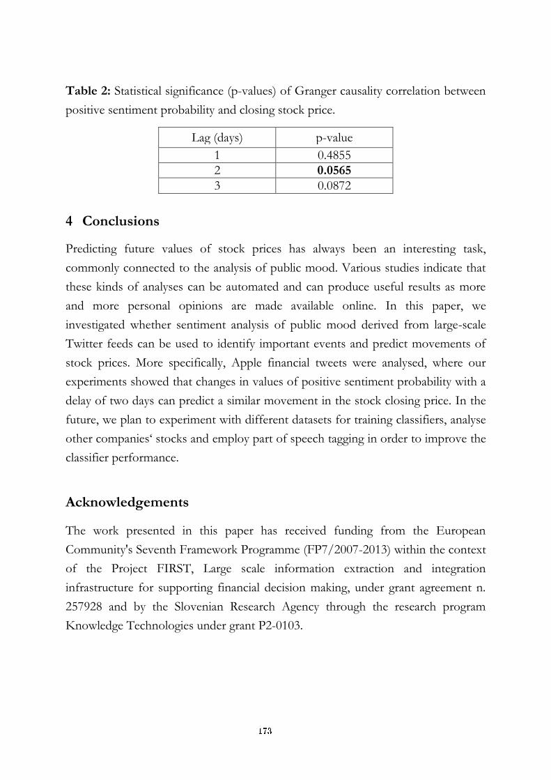
Table 2: Statistical significance (p-values) of Granger causality correlation between
positive sentiment probability and closing stock price.
Lag (days) p-value
1 0.4855
2 0.0565
3 0.0872
4 Conclusions
Predicting future values of stock prices has always been an interesting task,
commonly connected to the analysis of public mood. Various studies indicate that
these kinds of analyses can be automated and can produce useful results as more
and more personal opinions are made available online. In this paper, we
investigated whether sentiment analysis of public mood derived from large-scale
Twitter feeds can be used to identify important events and predict movements of
stock prices. More specifically, Apple financial tweets were analysed, where our
experiments showed that changes in values of positive sentiment probability with a
delay of two days can predict a similar movement in the stock closing price. In the
future, we plan to experiment with different datasets for training classifiers, analyse
other companies‘ stocks and employ part of speech tagging in order to improve the
classifier performance.
Acknowledgements
The work presented in this paper has received funding from the European
Community's Seventh Framework Programme (FP7/2007-2013) within the context
of the Project FIRST, Large scale information extraction and integration
infrastructure for supporting financial decision making, under grant agreement n.
257928 and by the Slovenian Research Agency through the research program
Knowledge Technologies under grant P2-0103.
173
References:
[1] P. Turney. Thumbs Up or Thumbs Down? Semantic Orientation Applied to Unsupervised Classification of Reviews. In Proceedings of the Association for Computational Linguistics, p. 417–424, 2002.
[2] E. Fama. Random Walks in Stock Market Prices. Financial Analysts Journal, 21(5): 55–59, 1965.
[3] K. C. Butler, S.J. Malaikah. Efficiency and inefficiency in thinly traded stock markets: Kuwait and Saudi Arabia. Journal of Banking and Finance 16, 197–210, 1992.
[4] M. Kavussanos, E. Dockery. A Multivariate test for stock market efficiency: The case of ASE. Applied Financial Economics, 11(5): 573-579, 2001.
[5] D. Gruhl, R. Guha, R. Kumar, J. Novak and A. Tomkins. The predictive power of online chatter. In Proceedings of the eleventh ACM SIGKDD international conference on Knowledge discovery in data mining, p. 78-87, New York, USA, 2005.
[6] G. Mishne and N. Glance. Predicting Movie Sales from Blogger Sentiment. In AAAI Symposium on Computational Approaches to Analysing Weblogs AAAI-CAAW, p. 155-158, 2006.
[7] S. Asur and B. A. Huberman. Predicting the Future with Social Media. In Proceedings of the ACM International Conference on Web Intelligence, arXiv:1003.5699v1, 2010.
[8] J. R. Nofsinger. Social Mood and Financial Economics. Journal of Behavioral Finance, 6(3): 144-160, 2005.
[9] J. Bollen, H. Mao, X. Zeng. Twitter mood predicts the stock market. Journal of Computational Science, 2(1): 1-8, 2011.
[10] A. Go, R. Bhayani, L. Huang. Twitter Sentiment Classification using Distant Supervision. Association for Computational Linguistics, p.30-38, 2009.
[11] T. Joachims. Training Linear SVMs in Linear Time. In Proceedings of the ACM Conference on Knowledge Discovery and Data Mining (KDD), 2006.
[12] A. Broder, S. Glassman, M. Manasse and G. Zweig. Syntactic Clustering of the Web. In Proceedings of WWW6 and Computer Networks 29:8-13, 1997.
[13] P. Wessa. Bivariate Granger Causality (v1.0.0) in Free Statistics Software (v1.1.23-r7), Office for Research Development and Education, http://www.wessa.net/rwasp_grangercausality.wasp/
174

For wider interest
From psychological research it is known that emotions are essential to rational
thinking. Also, it has been shown that the stock market is a direct reflection of the
social mood. On the other hand, more and more people make their opinions
available publicly online, making it available for analysis. Can we expect that the
analysis of public mood can identify important events and predict the movement of
stock market values? Our preliminary studies indicate that the answer is – yes. We
analysed the Apple financial Twitter posts that were collected in a 10 months
period. We identified days when people intensively talked about Apple and
consequently identified important events for this company. Next, we performed
statistical analysis for the period of specific 3 months, which is the period of the
main changes in the stock price, to determine whether we can predict future
movement of Apple`s closing price. The test showed that we are able to predict the
rise or fall in closing price two days before it occurs. This kind of analysis can also
be applied to other domains. For example, it can be used for the assessment of
products, prediction of purchase decisions, earnings and other similar phenomena.
175
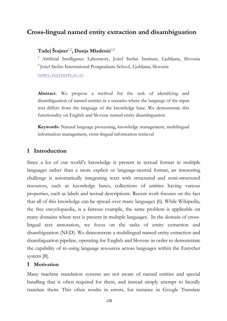
Cross-lingual named entity extraction and disambiguation
Tadej Štajner1,2, Dunja Mladenić1,2 1 Artificial Intelligence Laboratory, Jožef Stefan Institute, Ljubljana, Slovenia
2 Jožef Stefan International Postgraduate School, Ljubljana, Slovenia
Abstract. We propose a method for the task of identifying and
disambiguation of named entities in a scenario where the language of the input
text differs from the language of the knowledge base. We demonstrate this
functionality on English and Slovene named entity disambiguation
Keywords: Natural language processing, knowledge management, multilingual
information management, cross-lingual information retrieval
1 Introduction
Since a lot of our world’s knowledge is present in textual format in multiple
languages rather than a more explicit or language-neutral format, an interesting
challenge is automatically integrating texts with structured and semi-structured
resources, such as knowledge bases, collections of entities having various
properties, such as labels and textual descriptions. Recent work focuses on the fact
that all of this knowledge can be spread over many languages [6]. While Wikipedia,
the free encyclopaedia, is a famous example, the same problem is applicable on
many domains where text is present in multiple languages. In the domain of cross-
lingual text annotation, we focus on the tasks of entity extraction and
disambiguation (NED). We demonstrate a multilingual named entity extraction and
disambiguation pipeline, operating for English and Slovene in order to demonstrate
the capability of re-using language resources across languages within the Enrycher
system [8].
1 Motivation
Many machine translation systems are not aware of named entities and special
handling that is often required for them, and instead simply attempt to literally
translate them. This often results in errors, for instance in Google Translate
176

changing the name of the music band “Foo Fighters” into “Sigur Ros”, an
Icelandic music band, when translating from English to Icelandic. This illustrates
the need for special handling of proper names when doing machine translation. By
performing named entity extraction and disambiguation before translation, we are
able to use a knowledge base to find a correct translation for that named entity.
The second problem comes up in performing NED in a language that has poor
domain coverage in the knowledge base. Consequently, entities that are extracted
are not correctly disambiguated, since they don’t exist in that particular language.
However, the entity that we are looking for can exist in the knowledge base in a
different language. However, directly using that language introduces new problems,
since many of the components assume that the language of the input text
corresponds to the language of the knowledge base labels and descriptions.
2 Related work
The simplest solution for cross-lingual entity disambiguation is the one that simply
disregards the language mismatch and tries to use the full textual content to
perform the context similarity without any additional processing [1]. The authors
have shown that using a merged bilingual knowledge base performed significantly
better than using just the document language knowledge base, mainly due to better
domain coverage, but it performed much worse than a monolingual scenario.
Another simple baseline uses the equivalent of just using the context-independent
‘mention popularity’ measure, backed by a dictionary [2]. The dictionary can be
constructed from looking at anchor texts from non-English to English Wikipedia
pages. An ideal system would be the one that would simply translate the document
in the desired language and do the disambiguation on the translation. While doing
so manually is not feasible for our task, one may use machine translation to do this
[6]. While they achieve up to 94% performance of a monolingual baseline, machine
translation greatly complicates and slows down the processing, opening an window
for more efficient approaches.
3 Problem description
We state the problem as identifying and disambiguating concepts that appear as
mentions within a fragment of text. Disambiguation is important because phrases
may have many distinct meanings. While human readers are able to infer the
177

meaning from context, this task is difficult for computers. For instance, the phrase
“Washington” can be either a person, location or an organization, and even
constraining its type to a location yields over sixty possible different location that
are named that way.
3.1 Named entity extraction
Named entity extraction is the task of using the surrounding context to isolate the
part of text which represents an entity, referred to by a proper name. It is often
coupled with entity classification, determining to what class it belongs to, for
instance a person or an organization. In general, these are implemented as
supervised sequence classifiers.
3.2 Named entity disambiguation
Ambiguities, which are inherently present in natural languages represent a challenge
of determining the actual identities of entities mentioned in a document (e.g., Paris
can refer to a city in France but it can also refer to a small city in Texas, USA or to
a 1984 film directed by Wim Wenders having title Paris, Texas).
Well-defined entities and relationships are a property of the knowledge model
which asserts that a single term has only a single meaning. In that case, we refer to
terms as entities. We achieve this property by performing entity resolution. In
general, state of the art entity disambiguation systems use three main heuristics:
Mention popularity captures the overall most likely meanings of entity
phrases. It is typically modelled by the conditional probability of the named
entity given a mention.
Context similarity: This heuristic captures the entity that best fits the
topical context around the mention. It is modelled by the similarity of the
mention’s context and the entity’s context, using a similarity measure
operating on a bag-of-words model. The mention’s context is a window of
words around the mention in the input text, and the entity’s context is its
description.
Coherence: This heuristic collectively captures the entities that make sense
appearing together because they are somehow related to one another. While
context similarity operates on a single mention-entity pair, the coherence
heuristic is collective, operating on the whole input document. It is typically
solved by a greedy graph pruning algorithm.
178
3.3 Cross-lingual named entity disambiguation
When extending this pipeline into a scenario where the input and the knowledge
base are represented in multiple languages, the biggest impact of this change is on
the context similarity heuristic. Because it operates on the level of lexical similarity,
its output has little meaning when the assumption of a single language is removed.
4 Proposed method
We propose a method that incorporates a cross-lingual similarity measure into the
framework. Instead of just computing literal context similarity between two
contexts of different languages, we use an additional linear mapping that is able to
map one vector of bag-of-words features into another such vector in another
language. This enables us to perform meaningful similarity computation on the
same vector space.
The method used in this approach is Regression Canonical Correlation Analysis
(rCCA), a dimensionality reduction technique operation on two views that finds a
linear combination of vectors from both views (languages) that are maximally
correlated. The first vector corresponds to the input document, while the second
one corresponds to the optimal mapping of it. However, instead of calculating this
mapping in advance, we solve the optimization problem for each input document
separately around the input document as the initial projection vector.
Figure 1: The setup of obtaining similarity in cross-lingual NED
Figure 1 represents the two ways of obtaining a context similarity measure between
an input document and one of the candidate entities. When the languages of the
input and the knowledge base are the same, we use direct similarity. When they
differ, we first try to map the cross-lingual mapping (green triangle) into a vector
Input text
Knowledge base Mapped
text
Entity Direct similarity
Cross similarity
Cross-
lingual
mapping
179
space, compatible with the knowledge base. However, using a cross-lingual
mapping exposes us to the risk of poor domain coverage. Initial experiments show
that because the cross-lingual mapping was not able to map some of the words
from the input document, it will have poor performance. Therefore, we interpolate
the cross-similarity with the direct similarity with the proportion of the words that
the cross-lingual mapping was able to recognize. In pre-processing, we use the
Stanford Named Entity Recognizer [9] for English named entity recognition. For
Slovene, we have developed a Slovene named entity recognizer using a CRF
(Conditional random fields) model trained on the SSJ-500k corpus [9].
5 Discussion and conclusions
Current preliminary experiments show that obtaining a cross-lingual mapping does
improve on the context-similarity based NED when the training corpus and the
input text share a common topic. However, it is not yet certain whether it
compares favourably to a machine translation based system. Current work
demonstrates that the interpolation between direct and cross-lingual similarity help
the robustness of the systems. Future work will involve evaluating different cross-
lingual similarity models, as well as transliteration models and data integration
issues that arise when dealing with multilingual knowledge bases.
References:
[1] A. Lommatzsch et al, Named Entity Disambiguation for German News Articles, WIR 2010
[2] Spitkovsky, V.I. and Chang, A.X., Strong baselines for cross-lingual entity linking, TAC 2011
[3] T. Štajner and D. Mladenić: Entity resolution in texts using statistical learning and ontologies, ASWC 2009
[4] J. Rupnik, B. Fortuna. Regression Canonical Correlation Analysis. Learning from Multiple Sources, NIPS Workshop, 2008
[5] Hoffart, J., Yosef, M.A., Bordino, I., Fürstenau, H, Pinkal, M., Spaniol, M., Taneva, B., Thater, S., Weikum, G. (2011). Robust Disambiguation of Named Entities in Text. Proceedings of the 2011 Conference on Empirical Methods in Natural Language Processing, 782-792.
[6] McNamee, P., Mayfield, J., Oard, D. W., Lawrie, D., & Doermann, D. (2011). Cross-Language Entity Linking. IJCNLP 2001, 255-263.
[7] Učni korpus “Sporazumevanje v Slovenskem Jeziku”, http://www.xn--slovenina-qfb73g.eu/Vsebine/Sl/Aktivnosti/UcniKorpus.aspx, April 2012
[8] Štajner, T., Rusu, D., Dali, L., Fortuna, B., Mladenić, D., Grobelnik, M. A service oriented framework for natural language text enrichment. Informatica (Ljublj.), 2010, vol. 34, no. 3, 307-313. http://enrycher.ijs.si
[9] Jenny Rose Finkel, Trond Grenager, and Christopher Manning. 2005. Incorporating Non-local Information into Information Extraction Systems by Gibbs Sampling. Proceedings of the 43nd Annual Meeting of the ACL (ACL 2005), pp. 363-370.
180

For wider interest
When attempting to understand text, one of the tasks that need to be solved is
named entity disambiguation: for instance, Paris can refer to a city in France but it
can also refer to a small city in Texas, USA or to a 1984 film directed by Wim
Wenders having title Paris, Texas. Knowing the correct answer to that depends on
the context. However, context is difficult to interpret if the input text is expressed
in a different language than the knowledge base that these entities belong to.
This is a very common scenario in processing Slovene text. While using the Slovene
Wikipedia for this purpose is easy, it does not contain many entities that we may be
interested in. While the English one is over thirty times bigger, it introduces a
language barrier. We overcome this by applying techniques from cross-lingual
information retrieval to the problem of identifying proper names in text and linking
them to concrete knowledge base concepts.
Another goal was to re-use language resources from languages with more resource
in languages with less available resources. The work presented has resulted in a
usable named entity extraction and disambiguation service that is able to work on
Slovene text even while having a knowledge base in English.
The demonstration is available at http://enrycher.ijs.si
181
Extending the Multi-Criteria Decision Making Method DEX
Nejc Trdin 1,2, Marko Bohanec 1
1 Jožef Stefan Institute, Department of Knowledge Technologies, Ljubljana,
Slovenia
2 Jožef Stefan International Postgraduate School, Ljubljana, Slovenia
{nejc.trdin, marko.bohanec}@ijs.si
Abstract. The purpose of this work is to propose a plan for future research
and development of the qualitative decision support method DEX. DEX is a
qualitative multi-attribute modelling method used to evaluate and analyse
multiple decision alternatives in order to select the best alternative. We
propose six extensions to DEX: supporting full hierarchies, using numeric
attributes, probabilistic and fuzzy evaluations, general aggregation functions,
modularization and using relational models. These will be implemented in a
new decision support platform.
Keywords: Decision making, decision support, DEX, probability, fuzzy logic,
aggregation functions, modularization, relational models.
1 Introduction
People are able to make simple decisions very quickly, but are prone to making
sub-optimal decisions when facing a complex decision. Decision making can be
supported by appropriate techniques [1, 2]. One of such techniques is DEX [3, 4], a
qualitative decision modelling method. DEX was successfully used in many applications
such as ecology, industry and health care [5, 6, 7].
The motivation for this work follows from the observed needs for new
functionalities in practical applications. We propose six possible extensions of
DEX that will be further investigated and implemented in the future. In the
following, we first describe the DEX methodology (section 2) and then propose
the extensions (section 3). Section 4 concludes the work.
182
2 The DEX methodology
Decision making is a process which involves evaluating multiple alternatives, in order
to select the best alternative. The selected alternative should satisfy the goals of the
decision maker [1, 2, 4].
DEX is a representative of qualitative multi-attribute decision support methods [2, 3, 4]. Its
main property is that the observed attributes are represented with qualitative
attributes. The model developed using DEX methodology is described as a hierarchy
of attributes. The input attributes are at the lowest level, all other (aggregated)
attributes are concepts that logically depend on lower level attributes. Each
hierarchy has one or more special nodes, the root node(s), that have no parents. The
value given to the root nodes represent the final evaluations of the alternative. The
main difference between DEX and other multi-attribute methods is in the
aggregation functions, which are rules evaluating alternatives - each aggregated attribute
has one function. Aggregation functions in DEX are represented as tables.
A model developed according to these rules can be used to evaluate alternatives.
Alternatives’ values are assigned to the lowest attributes of the hierarchy. The
evaluation is done in a bottom-up fashion, using aggregation functions. The model
is also typically used for the analysis of decision alternatives, such as what-if analysis.
DEX is implemented in the software named DEXi [4, 8]. Also, there are some
other programs that implement extensions to the basic methodology:
proDEX [9]: Motivated by demands in ecological modelling [10], proDEX
implements probabilistic evaluation of alternatives. The final result of evaluation
is a probability distribution over the values of the root attribute.
Model revision [11]: This is a process of creating a new model from an existing
model and newly acquired data. The methodology revises the model by
modifying probabilities of rules in the model, without affecting the structure of
the model.
HINT [12]: This is a method for constructing DEX models from data. The
approach is based on function decomposition. HINT is a representative of concept
machine learning methods.
183
3 Proposed extensions to DEX methodology
DEX methodology is evidently very understandable, easy to use and yet strong
enough to assess complex decisions. However, further improvements are needed
due to practical requirements. In the following, we propose six possible extensions
to DEX methodology.
Supporting full hierarchies. In principle, the structure of the DEX model is a hierarchy,
i.e., directed acyclic graph. So far, hierarchies were only indirectly supported in
DEX [3] and DEXi software [8], using the concepts called “chaining” and
“linking” of nodes. In the extension we wish to fully support hierarchies by
representing them using the native graph form. Hierarchies also natively support
multiple root attributes.
Numeric attributes. Currently, DEX models employ only qualitative (symbolic)
attributes. The goal is to facilitate models that could simultaneously include both
qualitative and quantitative attributes. This means that we have to design principles of
including numeric attributes into DEX models. This extension is useful in
situations where attributes are better described with numeric values, rather than
symbolic; for example experts’ preference, salary, etc. Numeric values should be
used both to describe the properties of decision alternatives and decision makers’
preferences according to those properties. Some advances on introducing numeric
attributes into DEX are considered in [10, 13]. The main problem here is to
introduce mechanisms for conversion and mapping of both types of attributes.
Probabilistic and fuzzy evaluations. The notion of probabilistic computation is needed
for uncertain problem definitions. Actually, we would like to support both
probabilistic and fuzzy computations. Another generalization would be that
alternative input attributes would not only support crisp values, but also
distributions of values. The problem with supporting both probability and fuzzy
logic is combining both in the model, because computations are done differently.
General aggregation functions. With the introduction of numeric attributes, probabilities
and fuzziness, we will also have to adapt aggregation functions. Functions will have
184
to be able to compute with combinations of probabilities, fuzzy, symbolic and
numeric values. Adding numeric attributes will require adding a whole new set of
numeric aggregation functions. One of the main features of the aggregation
function is the ability to extract information from the end-user with as low effort as
possible. Furthermore, representations of aggregation functions must be
comprehensible to the user. Another extension is the capability for functions to
receive arbitrary number of inputs – functions such as sum, min, max, etc. The next
way to generalize functions is using the current tables, by constructing similar tables
with outputs dependant on the non-qualitative attributes. The main problem with
this generalization is that the function must be able to adapt when adding or
removing direct descendant attributes. The implementation must preserve as much
information as possible when doing operations on the model structure.
Modularization. Modularization means to merge a part of the model into one module,
which looks like an aggregated attribute. The newly created attribute would have
the same inputs and outputs as the part of the model before merging. Grouping
can be done in more levels, which leads to a tree-like structure of modules and
attributes. This means that, in addition to the hierarchical model structure, we need
to deal with another structure describing the grouping of attributes and modules.
The modularization technique is useful in managing big models, which are hard to
deal with. When a user completes a big part of some sub hierarchy, he would create
a module from this sub hierarchy and use it in other decision models; this improves
the reusability of developed components.
Relational models. Currently, DEX is capable of evaluating “flat” alternatives, that is,
alternatives described by a vector of values. In reality, however, alternatives may be
more complex. For example, we can have a company that is composed of
departments; in order to assess the company, we have to evaluate each department
separately and the company as a whole. We say that such an alternative is relational.
We also encounter relational alternatives in group decision making, where all the
decision makers have different preferences on the same matter - the matter can be
treated as some part of the sub hierarchy. The top aggregation function, where the
combination of all sub-model evaluations are combined, is the most important - the
aggregation is not constrained just to calculating to simple functions, but it can
185
have more complex structure. Similar technique was already implemented in DEX
software as “groups”, but in a limited fashion.
4 Conclusion
The primary contribution of this work was to propose possible extensions and
generalization of the DEX methodology. Six extensions were proposed, which will
considerably extend the functionality of the approach and facilitate addressing the
most complex decision problems encountered to date in practice. These extensions
will be further developed and implemented in a new software package with large
capabilities.
References:
[1] S. French. Decision Theory: An introduction to the Mathematics of Rationality. Halsted Press, 1986.
[2] D. Bouyssou, T. Marchant, M. Pirlot, A. Tsoukias and P. Vincke. Evaluation and Decision Models with Multiple Criteria. Springer, 2006.
[3] M. Bohanec and V. Rajkovič. DEX: An expert system shell for decision support. Sistemica, 1(1):145-157, 1990.
[4] M. Bohanec. Odločanje in Modeli. DMFA, 2006.
[5] M. Bohanec and V. Rajkovič. Multi-attribute decision modeling: Industrial applications of DEX. Informatica, 23(4):487-491, 1999.
[6] M. Bohanec, B. Zupan and V. Rajkovič. Applications of qualitative multi-attribute decision models in health care. International Journal of Medical Informatics, 58-59:191-205, 2000.
[7] M. Bohanec, S. Džeroski, M. Žnidaršič, A. Messeean, S. Scatasta and J. Wesseler. Multi-attribute modelling of economic and ecological impacts of cropping systems. Informatica, 28(4):387-392, 2004.
[8] DEXi: A program for multi-attribute decision making. http://kt.ijs.si/MarkoBohanec/dexi.html, 2012.
[9] M. Žnidaršič, M. Bohanec. Handling uncertainty in DEX methodology. In URPDM 2010: Proceedings of the 25th Mini-EURO Conference, Coimbra, Portugal, 2010.
[10] M. Žnidaršič, M. Bohanec and B. Zupan. Modelling impacts of cropping systems: Demands and solutions for DEX methodology. European Journal of Operational Research, 189(3):594-608, 2008.
[11] M. Žnidaršič and M. Bohanec. Data-based revision of probability distributions in qualitative multi-attribute decision models. Intelligent Data Analysis, 9(2):159-174, 2005.
[12] B. Zupan, M. Bohanec, J. Demšar and I. Bratko. Learning by discovering concept hierarchies. Articial Intelligence, 109(1-2):211-242, 1999.
[13] M. Žnidaršič, M. Bohanec and I. Bratko. Categorization of numerical values for DEX hierarchical models. Informatica, 27(4):405-409, 2003.
186
For wider interest
The main purpose of this paper is to propose six new extensions to the DEX
methodology. The methodology is a member of multi-attribute decision support
techniques, which are used for supporting people at making better decisions.
Usually such decisions are made in business environments, ecology, industry and
also in personal decisions, e. g., choosing a family vehicle.
A DEX decision model is constructed as a hierarchy of attributes, which are
connected in a logical sense. For example, when choosing a car, one would logically
construct “maintenance price” from “buying price” and “consumption”. The
attributes used in the hierarchy are presented as qualitative (symbolic) values. The
values are not presented as numerical (-1, 0.12, 18, …), but rather as “good”,
“medium” and “bad”. This is particularly useful in decision situations where
judgement prevails over exact formal treatment of criteria.
As written in the paper, the methodology was successfully used in many different
applications, but still lacks some functionality for the decision maker. Three useful
extensions were developed before, but there are still more functionalities needed
from the system.
Our goal is to successfully design, investigate and finally implement six additional
extensions to the DEX methodology in a new powerful decision support system.
The presented extensions are related to the model structure (supporting full
hierarchies), attribute representation (facilitating probabilistic and fuzzy
computations, and numeric attributes), model representation (introducing
modularization), aggregation functions (supporting general aggregation functions)
and support for relational models.
187
Development of Discovery and Identification Protocol for Sensor Networks
Matevž Vučnik1,2, Zoltan Padrah1,2, Carolina Fortuna1,2, Mihael Mohorčič1,2
1 Department of Communication Systems, Jožef Stefan Institute, Ljubljana, Slovenia
2 Jožef Stefan International Postgraduate School, Ljubljana, Slovenia
{matevz.vucnik, zoltan.padrah, carolina.fortuna, miha.mohorcic}@ijs.si
Abstract. This paper describes a new application layer communication
protocol Discovery and Identification Protocol (DIP). The DIP protocol is
designed to be used in low power wireless sensor networks (WSN) for
discovery of the sensor nodes and sensor data collection. We first describe the
design of the protocol and then the implementation of the protocol in the
event based operating system Contiki, which targets extremely low power
devices such as sensor nodes. In the conclusion we give a comparison of DIP
and Constrained Application Protocol (CoAP) which is an application
communication protocol with a more general design enabling the evolution of
the current Web to the “Web of Things”.
Keywords: WSN, communication, discovery, web, measurements, metadata.
1 Introduction
Sensor data collection is one of the most important components in Wireless Sensor
Networks (WSN). With sensor data we refer to (1) sensor measurements which are
typically represented with a simple float number with a changing value, with
exceptions such as cameras, where the output is an image or a video, and (2) the
metadata, which gives the meaning to the measurement and normally does not
change over time. The metadata consists of all the information about the
measurement starting with measurement unit, accuracy, calibration parameters, etc.
to contextual description of environment where the measurements were collected
(e.g. environment characteristics, etc.). The measurements are normally significantly
smaller than the metadata, but they change over time and need to be retrieved more
frequently.
188
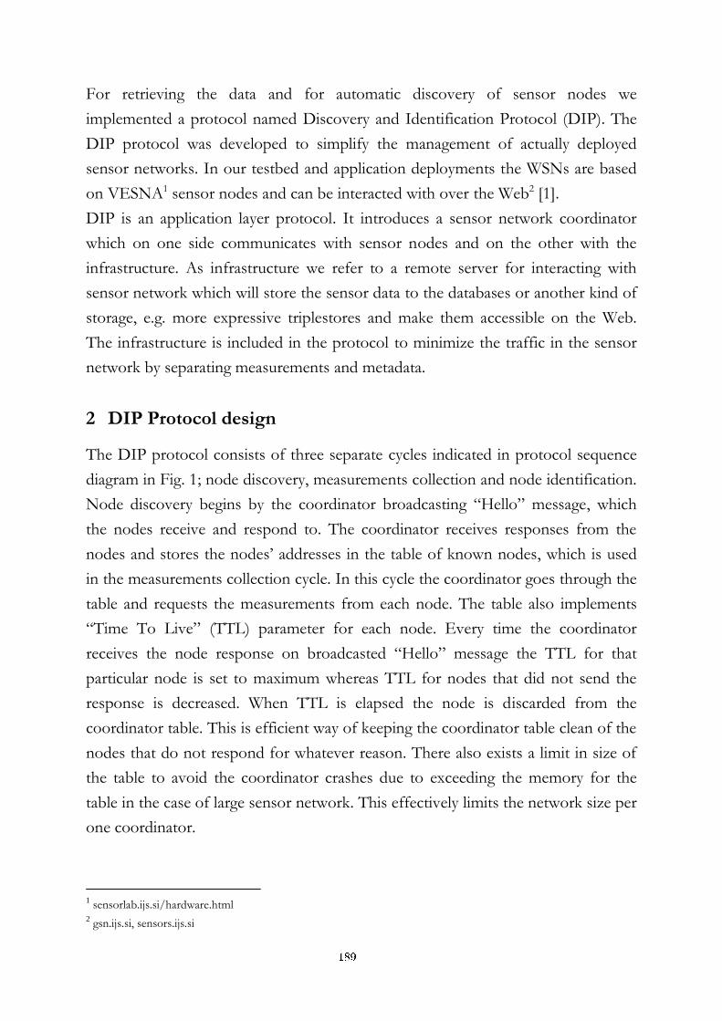
For retrieving the data and for automatic discovery of sensor nodes we
implemented a protocol named Discovery and Identification Protocol (DIP). The
DIP protocol was developed to simplify the management of actually deployed
sensor networks. In our testbed and application deployments the WSNs are based
on VESNA1 sensor nodes and can be interacted with over the Web2 [1].
DIP is an application layer protocol. It introduces a sensor network coordinator
which on one side communicates with sensor nodes and on the other with the
infrastructure. As infrastructure we refer to a remote server for interacting with
sensor network which will store the sensor data to the databases or another kind of
storage, e.g. more expressive triplestores and make them accessible on the Web.
The infrastructure is included in the protocol to minimize the traffic in the sensor
network by separating measurements and metadata.
2 DIP Protocol design
The DIP protocol consists of three separate cycles indicated in protocol sequence
diagram in Fig. 1; node discovery, measurements collection and node identification.
Node discovery begins by the coordinator broadcasting “Hello” message, which
the nodes receive and respond to. The coordinator receives responses from the
nodes and stores the nodes’ addresses in the table of known nodes, which is used
in the measurements collection cycle. In this cycle the coordinator goes through the
table and requests the measurements from each node. The table also implements
“Time To Live” (TTL) parameter for each node. Every time the coordinator
receives the node response on broadcasted “Hello” message the TTL for that
particular node is set to maximum whereas TTL for nodes that did not send the
response is decreased. When TTL is elapsed the node is discarded from the
coordinator table. This is efficient way of keeping the coordinator table clean of the
nodes that do not respond for whatever reason. There also exists a limit in size of
the table to avoid the coordinator crashes due to exceeding the memory for the
table in the case of large sensor network. This effectively limits the network size per
one coordinator.
1 sensorlab.ijs.si/hardware.html
2 gsn.ijs.si, sensors.ijs.si
189
Our measurements collection protocol running on the coordinator node pulls the
measurements from the nodes found in the table and pushes them towards the
infrastructure, unaware if the server knows the measuring nodes. The coordinator
waits for the infrastructure response and in case the infrastructure does not know a
given node it sends a request for identification of that node to the coordinator.
Upon request the coordinator demands the metadata from the node and forwards
it to the infrastructure (see Fig. 1). Metadata gives meaning to the measurements so
they can be used in various applications.
Coordinator Node_1 Node_2Infrastructure
Discovery
Measurements
collection
Identification
U
B
B
B
U
U
S
S
S
U
U
S
S
U
S U
US
U
US
S U
US
“Hi”
“Hi”
“Hi”
“Measurements?”
“Measurements”
“Measurements?”
“Measurements”
“Measurements”
“Identification not needed”
“Identification not needed”
“Measurements?”
“Measurements?”
“Measurements”
“Measurements”“Measurements”
“Identification needed”
“Identification needed”
“Metadata?”
“Metadata”“Metadata”
“Metadata?”
“Metadata”“Metadata”
“Measurements”
B U S- Broadcast - Unicast - Implementation dependent
B “Hi”
Figure 1: The DIP sequence diagram
3 Implementation of DIP in Contiki operating system
For the implementation of DIP we used a VESNA sensor node platform running
the Contiki3 operating system. Contiki has a communication stack called RIME
which offers features like addressing, broadcast, reliable unicast and reliable bulk
3 www.contiki-os.org/
190
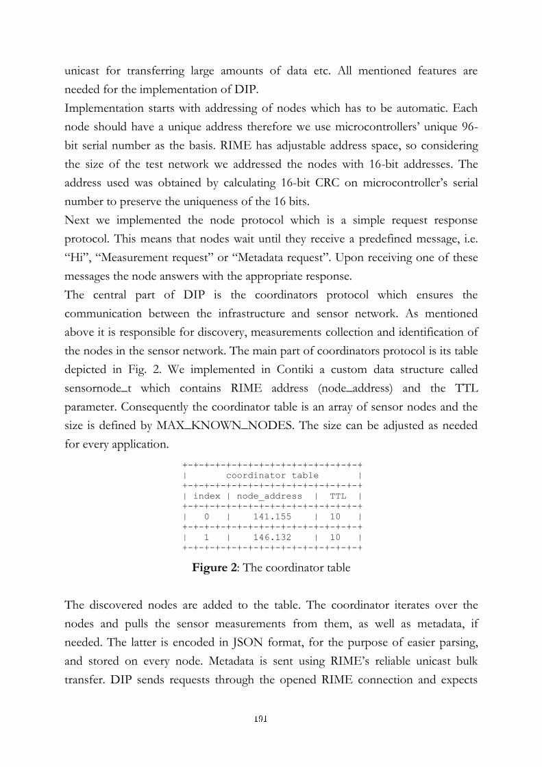
unicast for transferring large amounts of data etc. All mentioned features are
needed for the implementation of DIP.
Implementation starts with addressing of nodes which has to be automatic. Each
node should have a unique address therefore we use microcontrollers’ unique 96-
bit serial number as the basis. RIME has adjustable address space, so considering
the size of the test network we addressed the nodes with 16-bit addresses. The
address used was obtained by calculating 16-bit CRC on microcontroller’s serial
number to preserve the uniqueness of the 16 bits.
Next we implemented the node protocol which is a simple request response
protocol. This means that nodes wait until they receive a predefined message, i.e.
“Hi”, “Measurement request” or “Metadata request”. Upon receiving one of these
messages the node answers with the appropriate response.
The central part of DIP is the coordinators protocol which ensures the
communication between the infrastructure and sensor network. As mentioned
above it is responsible for discovery, measurements collection and identification of
the nodes in the sensor network. The main part of coordinators protocol is its table
depicted in Fig. 2. We implemented in Contiki a custom data structure called
sensornode_t which contains RIME address (node_address) and the TTL
parameter. Consequently the coordinator table is an array of sensor nodes and the
size is defined by MAX_KNOWN_NODES. The size can be adjusted as needed
for every application.
Figure 2: The coordinator table
The discovered nodes are added to the table. The coordinator iterates over the
nodes and pulls the sensor measurements from them, as well as metadata, if
needed. The latter is encoded in JSON format, for the purpose of easier parsing,
and stored on every node. Metadata is sent using RIME’s reliable unicast bulk
transfer. DIP sends requests through the opened RIME connection and expects
+-+-+-+-+-+-+-+-+-+-+-+-+-+-+-+-+
| coordinator table |
+-+-+-+-+-+-+-+-+-+-+-+-+-+-+-+-+
| index | node_address | TTL |
+-+-+-+-+-+-+-+-+-+-+-+-+-+-+-+-+
| 0 | 141.155 | 10 |
+-+-+-+-+-+-+-+-+-+-+-+-+-+-+-+-+
| 1 | 146.132 | 10 |
+-+-+-+-+-+-+-+-+-+-+-+-+-+-+-+-+
191
the response in a callback function which is called directly from the radio driver,
whereas the RIME stack introduces a more cross layer approach for
communication.
4 Conclusion and Future Work
In this paper we described the DIP protocol custom designed for discovery of the
sensor nodes and sensor data collection. The DIP protocol is suitable for narrow
field, special purpose applications requiring light-weight protocol stack
implementation. As an alternative to DIP, and more generally suitable for various
applications, a layered approach can be used assuming implementation of the whole
internet protocol suite from physical layer to application layer on the sensor node.
This includes IEEE 802.15.4 compliant radios used along with the multitasking
operating system Contiki, which implements protocols such as 6LoWPAN, IPv6,
UDP and CoAP, enabling the evolution of the current Web to the “Web of
Things” [2]. The Contiki OS implements all the necessary communication layers
and corresponding protocols to have CoAP working on top of it. The MAC layer is
already implemented inside the IEEE 802.15.4 compliant radio.
The IP protocol stack enables new applications similar to the ones in the current
Web, only running on small low power devices and forming the “Web of Things”.
With the newly developed CoAP framework in Java language called Californium
(Cf)4 new cloud services based on “Things” are possible [3].
References:
[1] M. Vučnik, C. Fortuna, M. Porcius, M. Mohorčič. WSN Testbeds For Lighting Control And Environmental Monitoring. In Proceedings of the 3rd Jožef Stefan International Postgraduate School Student’s Conference. Ljubljana, Slovenia, 2011
[2] M. Kovatsch. Demo abstract: Human-CoAP interaction with Copper. In Distributed Computing in Sensor Systems and Workshops (DCOSS), Barcelona, Spain, 2011.
[3] M. Kovatsch, S. Mayer, B. Ostermaier. Moving Application Logic from the Firmware to the Cloud: Towards the Thin Server Architecture for the Internet of Things. In Proceedings of the 6th International Conference on Innovative Mobile and Internet Services in Ubiquitous Computing (IMIS 2012), Palermo, Italy, 2012.
4 https://github.com/mkovatsc/Californium
192
For wider interest
This paper describes a new protocol which is useful for collecting sensor
measurements and metadata from sensor networks. The protocol is called
Discovery and Identification Protocol (DIP).
Sensor networks are increasingly used to deliver sensor data from the world or real
things and processes. Sensor data includes sensor measurements, which are samples
typically in the form of a number (e.g. temperature), and the metadata, which is
typically static information that gives meaning to the measurements (e.g. accuracy,
calibration parameters, sensor settings etc.).
The DIP protocol was designed as a light-weight protocol to be used on sensor
nodes which consume very little energy and can run on batteries. Sensor nodes are
connected to the network through a wireless interface.
The paper is divided into two parts where the first part describes the design of the
protocol and the second part describes the implementation of the protocol. In the
conclusion we give a comparison of DIP and another more general protocol called
Constrained Application Protocol (CoAP).
The protocols described enable the evolution of the current Web so as to include
also the “Web of Things”.
193


Nanoznanosti in nanotehnologije (Nanosciences and
Nanotechnologies)
195

Spectroscopic THz imaging using organic DSTMS (4-N,N-dimethylamino-4’-N’-methyl-stilbazolium 2,4,6-trimethylbenzenesulfonate) crystals
Andreja Abina1, Uroš Puc1, David Heath1, Aleksander Zidanšek1,2
1 Jožef Stefan International Postgraduate School, Ljubljana, Slovenia
2 Department of Condensed Matter Physics, Jožef Stefan Institute, Ljubljana,
Slovenia
Abstract. Application of terahertz (THz) electromagnetic waves offers several
opportunities for quality inspection in various industries. The THz waves
penetrate many kinds of materials such as pharmaceutical coating, paper,
plastic, ceramic, cardboard, wood, clothing, etc. We investigated possibilities
of applying a THz imaging system in transmission geometry using the organic
DSTMS crystals as a THz generator and detector. We applied different
methods to construct an image from the array of THz pulses. Time-domain
THz imaging has the advantage of the fast sample scanning. It is however
appropriate only for detection of imperfections or impurities inside the
material as well as for the thickness distribution measurement. For
identification of the observed substance multispectral imaging is necessary.
Keywords: Material characterization, Organic DSTMS crystals, THz
spectroscopy, THz imaging.
1 Introduction
Terahertz (THz) region of the electromagnetic spectrum was not well explored
until recently. This THz gap is located between infrared waves and microwaves
with corresponding wavelengths between 3 mm and 30 micro meters [1] as
depicted in Fig. 1. One of the most promising aspects of this new technology is its
high sensitivity to interactions between molecules and THz responses which exhibit
some interesting characteristics. The THz sensor is able to probe not only rotations
as in case of microwaves, but also the various intermolecular bonds such as
197
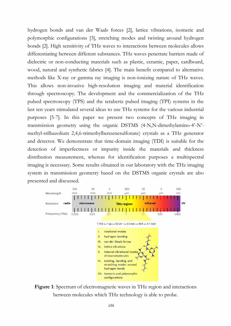
hydrogen bonds and van der Waals forces [2], lattice vibrations, isomeric and
polymorphic configurations [3], stretching modes and twisting around hydrogen
bonds [2]. High sensitivity of THz waves to interactions between molecules allows
differentiating between different substances. THz waves penetrate barriers made of
dielectric or non-conducting materials such as plastic, ceramic, paper, cardboard,
wood, natural and synthetic fabrics [4]. The main benefit compared to alternative
methods like X-ray or gamma ray imaging is non-ionizing nature of THz waves.
This allows non-invasive high-resolution imaging and material identification
through spectroscopy. The development and the commercialization of the THz
pulsed spectroscopy (TPS) and the terahertz pulsed imaging (TPI) systems in the
last ten years stimulated several ideas to use THz systems for the various industrial
purposes [5-7]. In this paper we present two concepts of THz imaging in
transmission geometry using the organic DSTMS (4-N,N-dimethylamino-4’-N’-
methyl-stilbazolium 2,4,6-trimethylbenzenesulfonate) crystals as a THz generator
and detector. We demonstrate that time-domain imaging (TDI) is suitable for the
detection of imperfectness or impurity inside the materials and thickness
distribution measurement, whereas for identification purposes a multispectral
imaging is necessary. Some results obtained in our laboratory with the THz imaging
system in transmission geometry based on the DSTMS organic crystals are also
presented and discussed.
Figure 1: Spectrum of electromagnetic waves in THz region and interactions
between molecules which THz technology is able to probe.
198
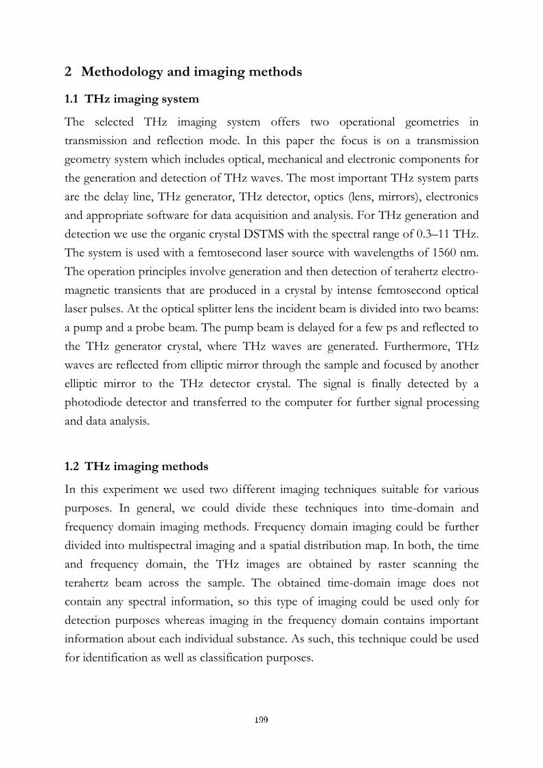
2 Methodology and imaging methods
1.1 THz imaging system
The selected THz imaging system offers two operational geometries in
transmission and reflection mode. In this paper the focus is on a transmission
geometry system which includes optical, mechanical and electronic components for
the generation and detection of THz waves. The most important THz system parts
are the delay line, THz generator, THz detector, optics (lens, mirrors), electronics
and appropriate software for data acquisition and analysis. For THz generation and
detection we use the organic crystal DSTMS with the spectral range of 0.3–11 THz.
The system is used with a femtosecond laser source with wavelengths of 1560 nm.
The operation principles involve generation and then detection of terahertz electro-
magnetic transients that are produced in a crystal by intense femtosecond optical
laser pulses. At the optical splitter lens the incident beam is divided into two beams:
a pump and a probe beam. The pump beam is delayed for a few ps and reflected to
the THz generator crystal, where THz waves are generated. Furthermore, THz
waves are reflected from elliptic mirror through the sample and focused by another
elliptic mirror to the THz detector crystal. The signal is finally detected by a
photodiode detector and transferred to the computer for further signal processing
and data analysis.
1.2 THz imaging methods
In this experiment we used two different imaging techniques suitable for various
purposes. In general, we could divide these techniques into time-domain and
frequency domain imaging methods. Frequency domain imaging could be further
divided into multispectral imaging and a spatial distribution map. In both, the time
and frequency domain, the THz images are obtained by raster scanning the
terahertz beam across the sample. The obtained time-domain image does not
contain any spectral information, so this type of imaging could be used only for
detection purposes whereas imaging in the frequency domain contains important
information about each individual substance. As such, this technique could be used
for identification as well as classification purposes.
199
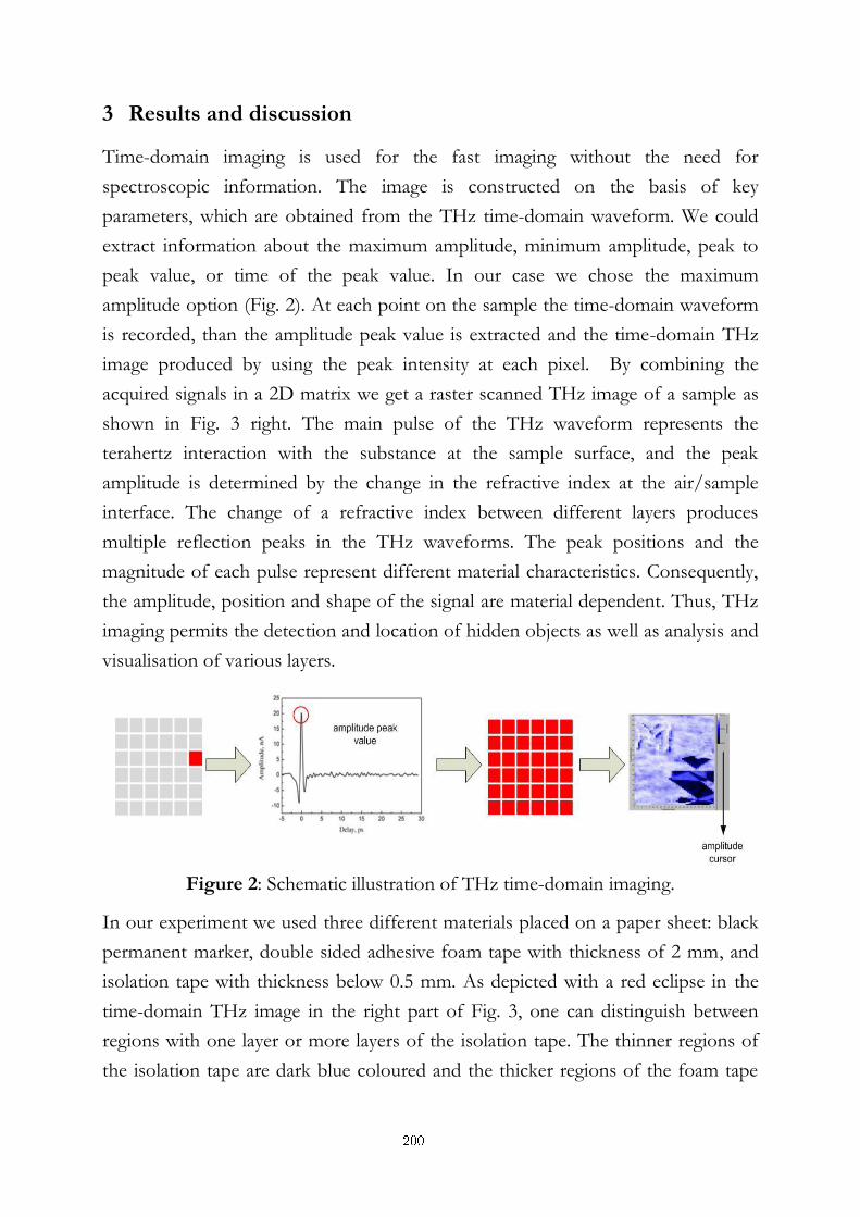
3 Results and discussion
Time-domain imaging is used for the fast imaging without the need for
spectroscopic information. The image is constructed on the basis of key
parameters, which are obtained from the THz time-domain waveform. We could
extract information about the maximum amplitude, minimum amplitude, peak to
peak value, or time of the peak value. In our case we chose the maximum
amplitude option (Fig. 2). At each point on the sample the time-domain waveform
is recorded, than the amplitude peak value is extracted and the time-domain THz
image produced by using the peak intensity at each pixel. By combining the
acquired signals in a 2D matrix we get a raster scanned THz image of a sample as
shown in Fig. 3 right. The main pulse of the THz waveform represents the
terahertz interaction with the substance at the sample surface, and the peak
amplitude is determined by the change in the refractive index at the air/sample
interface. The change of a refractive index between different layers produces
multiple reflection peaks in the THz waveforms. The peak positions and the
magnitude of each pulse represent different material characteristics. Consequently,
the amplitude, position and shape of the signal are material dependent. Thus, THz
imaging permits the detection and location of hidden objects as well as analysis and
visualisation of various layers.
Figure 2: Schematic illustration of THz time-domain imaging.
In our experiment we used three different materials placed on a paper sheet: black
permanent marker, double sided adhesive foam tape with thickness of 2 mm, and
isolation tape with thickness below 0.5 mm. As depicted with a red eclipse in the
time-domain THz image in the right part of Fig. 3, one can distinguish between
regions with one layer or more layers of the isolation tape. The thinner regions of
the isolation tape are dark blue coloured and the thicker regions of the foam tape
200
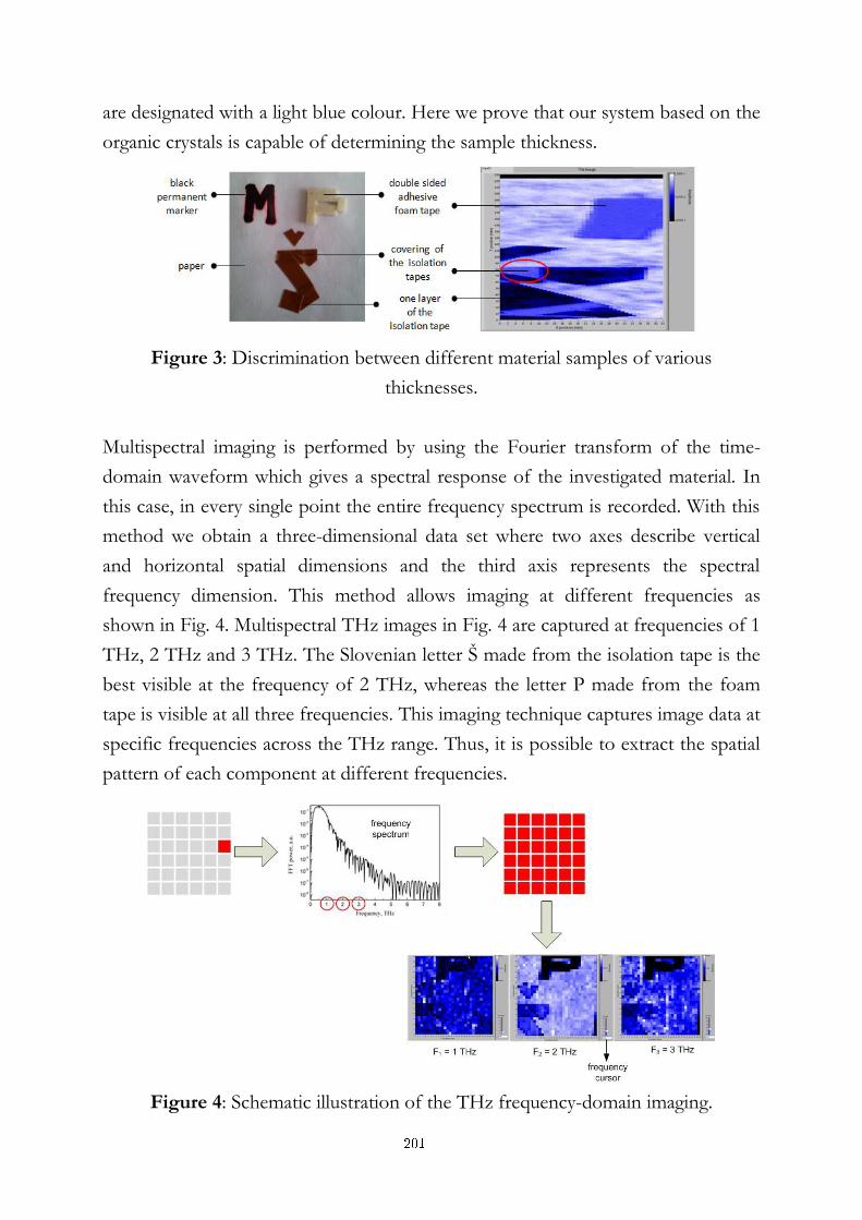
are designated with a light blue colour. Here we prove that our system based on the
organic crystals is capable of determining the sample thickness.
Figure 3: Discrimination between different material samples of various
thicknesses.
Multispectral imaging is performed by using the Fourier transform of the time-
domain waveform which gives a spectral response of the investigated material. In
this case, in every single point the entire frequency spectrum is recorded. With this
method we obtain a three-dimensional data set where two axes describe vertical
and horizontal spatial dimensions and the third axis represents the spectral
frequency dimension. This method allows imaging at different frequencies as
shown in Fig. 4. Multispectral THz images in Fig. 4 are captured at frequencies of 1
THz, 2 THz and 3 THz. The Slovenian letter Š made from the isolation tape is the
best visible at the frequency of 2 THz, whereas the letter P made from the foam
tape is visible at all three frequencies. This imaging technique captures image data at
specific frequencies across the THz range. Thus, it is possible to extract the spatial
pattern of each component at different frequencies.
Figure 4: Schematic illustration of the THz frequency-domain imaging.
201
4 Conclusions
Capability of spectroscopic discrimination is one of the most promising features of
the THz imaging system. On the one hand the acquired THz data contain rich
information about the structure and composition of a given sample. On the other
hand, the characteristic spectral signatures of each individual substance can also be
extracted from the THz data, and this can be used for substance identification. We
applied different methods to construct an image from the array of THz pulses.
Time-domain THz imaging has the advantage of a fast sample scanning at the
expense of lower resolution. Therefore, it is appropriate only for the detection of
some imperfections or impurities inside the investigated material and for the
thickness measurements, whereas for identification purposes the multispectral
imaging method is necessary. The Fourier transform of the measured THz signal
provides additional information about the investigated sample. Therefore, the
frequency characteristics of each point can be viewed and the material properties,
such as distribution of chemical compounds within the material, can be
determined.
References:
[1] Y.-C. Shen, P. F. Taday, D. A. Newnham, M. C. Kemp, and M. Pepper. 3D chemical mapping using terahertz pulsed imaging, In Proceedings of the SPIE 5727, 2005 .
[2] M. Walther, B. Fischer, A. Ortner, A. Bitzer, A. Thoman, and H. Helm. Chemical sensing and imaging with pulsed terahertz radiation, Analytical and Bioanalytical Chemistry, 397(3): 1009–1017, 2010.
[3] J. A. Zeitler, P. F. Taday, D. A. Newnham, M. Pepper, K. C. Gordon, and T. Rades. Terahertz pulsed spectroscopy and imaging in the pharmaceutical setting - a review, Journal of Pharmacy and Pharmacology, 59(2): 209–223, 2007.
[4] M. C. Kemp. Millimetre wave and terahertz technology for the detection of concealed threats: a review, In Proccedings of Joint 32nd International Conference on Infrared and Millimeter Waves, 2007 and the 2007 15th International Conference on Terahertz Electronics. IRMMW-THz, Cardiff, 2006.
[5] S. Yao-Chun and P. F. Taday. Development and Application of Terahertz Pulsed Imaging for Nondestructive Inspection of Pharmaceutical Tablet, IEEE Journal of Selected Topics in Quantum Electronics, 14(2): 407–415, 2008.
[6] E. Brundermann, U. Heugen, R. Schiwon, B. Born, G. W. Schwaab, S. Ebbinghaus, K. Schrock, D. R. Chamberlin, E. E. Haller, and M. Havenith. Terahertz imaging applications in spectroscopy of biomolecules, In IEEE MTT-S International Microwave Symposium Digest 2005, Long Beach, CA, 2005.
[7] C. Jansen, S. Wietzke, O. Peters, M. Scheller, N. Vieweg, M. Salhi, N. Krumbholz, C. Jördens, T. Hochrein, and M. Koch. Terahertz imaging: applications and perspectives, Applied Optics, 49(19): E48-E57, 2010.
202
For wider interest
Terahertz (THz) region of the electromagnetic spectrum was not well explored
until recently. This THz gap is located between infrared waves and microwaves at
corresponding wavelengths between 3 mm and 30 micro meters. One of the most
promising aspects of this new technology is its high sensitivity to interactions
between molecules and some interesting characteristics in THz spectrum. Since
THz waves are very sensitive to interactions between molecules this allows
discrimination between different substances. Moreover, the THz waves penetrate
barriers made of dielectric or non-conducting materials such as plastic, ceramic,
paper, cardboard, wood, natural and synthetic fabrics. Thus, the THz technology
presents an alternative method to X-ray or gamma ray imaging. The development
and commercialization of the terahertz pulsed spectroscopy (TPS) and terahertz
pulsed imaging (TPI) systems during the last decade put forward several ideas to
use the THz systems for various industrial purposes.
One of the most promising features of a THz imaging system is its capability for
spectroscopic discrimination. The acquired THz data contain rich information
about the structure and composition of a sample. On the other hand, the
characteristic spectral signatures of each individual substance can also be extracted
from the THz data, and this can be used for substance identification. In this work
we applied two concepts of the THz imaging in transmission geometry using
organic DSTMS crystals as a THz generator and detector. We demonstrate that the
time-domain THz imaging has the advantage of fast sample scanning at the
expense of lower resolution. Therefore, it is appropriate only for the detection of
some imperfections or impurities inside the investigated material and for thickness
measurements, whereas for substance identification the multispectral imaging
method is necessary. Fourier transform of the THz signal provides additional
information about the investigated sample. Therefore, the frequency characteristics
of each point can be viewed and the material properties, such as distribution of
chemical compounds within the material, can be determined.
203
Influence of different stress concentration factors in mono-leaf spring on its final fatigue life
Predrag Borković, Borivoj Šuštaršič, Vojteh Leskovšek, Borut Žužek
Institute of Metals and Technology, Ljubljana, Slovenia
Abstract. Fatigue life of a component is a very important information
regarding safety and stability of any dynamically loaded systems. Since the
failure under such loaded parts can occur even at lower stress than static
tensile strength, the fatigue life has to be assessed by simulations or by
performing tests on real components. Among many influencing factors on the
fatigue life, the influence of irregular stress flow expressed by the stress
concentration factor within the component is presented in this paper. Finite
Element Method (FEM) based simulations have showed a clear difference in
the fatigue life results by changing the transition radius of the mono-leaf
spring following the change of a stress concentration factor as well. These
FEM simulations are performed taking into account dynamic properties of the
spring steel obtained by tests on specimens.
Keywords: fatigue life, stress concentration factor, mono-leaf spring, FEM
simulation
1 Introduction
The estimation of the fatigue life by calculation is based on the global loading of
the components, the knowledge about the stresses in the component and the
behaviour of the material under dynamic loading [1]. For the stress determination,
numerical methods are used, e.g. the finite element method, while load spectra are
established by tests. The information about the strength behaviour of the material
is the third group of input data for the calculation of the fatigue life. Also,
influences of a different segregation orientation of alloying elements, a different
tempering temperature and a notch effect on fatigue life were examined. The input
data of the FEM based simulations are S/N curves, obtained by the fatigue tests on
specimens made of the same material as a mono leaf spring.
204
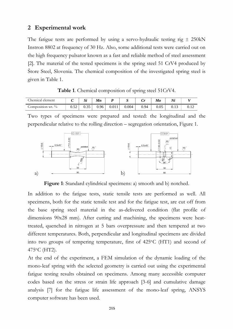
2 Experimental work
The fatigue tests are performed by using a servo-hydraulic testing rig ± 250kN
Instron 8802 at frequency of 30 Hz. Also, some additional tests were carried out on
the high frequency pulsator known as a fast and reliable method of steel assessment
[2]. The material of the tested specimens is the spring steel 51 CrV4 produced by
Štore Steel, Slovenia. The chemical composition of the investigated spring steel is
given in Table 1.
Table 1. Chemical composition of spring steel 51CrV4.
Two types of specimens were prepared and tested: the longitudinal and the
perpendicular relative to the rolling direction – segregation orientation, Figure 1.
a) b)
Figure 1: Standard cylindrical specimens: a) smooth and b) notched.
In addition to the fatigue tests, static tensile tests are performed as well. All
specimens, both for the static tensile test and for the fatigue test, are cut off from
the base spring steel material in the as-delivered condition (flat profile of
dimensions 90x28 mm). After cutting and machining, the specimens were heat-
treated, quenched in nitrogen at 5 bars overpressure and then tempered at two
different temperatures. Both, perpendicular and longitudinal specimens are divided
into two groups of tempering temperature, first of 425C (HT1) and second of
475C (HT2).
At the end of the experiment, a FEM simulation of the dynamic loading of the
mono-leaf spring with the selected geometry is carried out using the experimental
fatigue testing results obtained on specimens. Among many accessible computer
codes based on the stress or strain life approach [3-6] and cumulative damage
analysis [7] for the fatigue life assessment of the mono-leaf spring, ANSYS
computer software has been used.
Chemical element C Si Mn P S Cr Mo Ni V
Composition wt. % 0.52 0.35 0.96 0.011 0.004 0.94 0.05 0.13 0.12
205
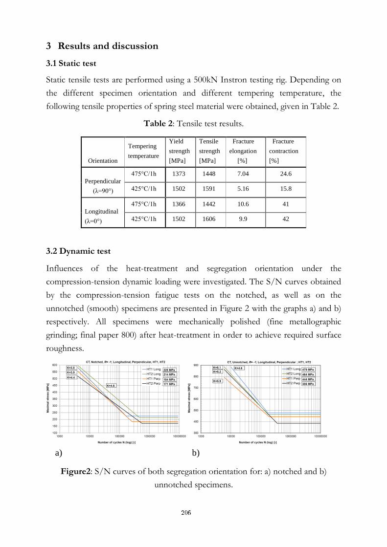
3 Results and discussion
3.1 Static test
Static tensile tests are performed using a 500kN Instron testing rig. Depending on
the different specimen orientation and different tempering temperature, the
following tensile properties of spring steel material were obtained, given in Table 2.
Table 2: Tensile test results.
3.2 Dynamic test
Influences of the heat-treatment and segregation orientation under the
compression-tension dynamic loading were investigated. The S/N curves obtained
by the compression-tension fatigue tests on the notched, as well as on the
unnotched (smooth) specimens are presented in Figure 2 with the graphs a) and b)
respectively. All specimens were mechanically polished (fine metallographic
grinding; final paper 800) after heat-treatment in order to achieve required surface
roughness.
a) b)
Figure2: S/N curves of both segregation orientation for: a) notched and b)
unnotched specimens.
Orientation
Tempering
temperature
Yield
strength
[MPa]
Tensile
strength
[MPa]
Fracture
elongation
[%]
Fracture
contraction
[%]
Perpendicular
(λ=90°)
475°C/1h 1373 1448 7.04 24.6
425°C/1h 1502 1591 5.16 15.8
Longitudinal
(λ=0°)
475°C/1h 1366 1442 10.6 41
425°C/1h 1502 1606 9.9 42
206
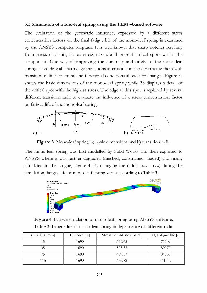
3.3 Simulation of mono-leaf spring using the FEM –based software
The evaluation of the geometric influence, expressed by a different stress
concentration factors on the final fatigue life of the mono-leaf spring is examined
by the ANSYS computer program. It is well known that sharp notches resulting
from stress gradients, act as stress raisers and present critical spots within the
component. One way of improving the durability and safety of the mono-leaf
spring is avoiding all sharp edge transitions at critical spots and replacing them with
transition radii if structural and functional conditions allow such changes. Figure 3a
shows the basic dimensions of the mono-leaf spring while 3b displays a detail of
the critical spot with the highest stress. The edge at this spot is replaced by several
different transition radii to evaluate the influence of a stress concentration factor
on fatigue life of the mono-leaf spring.
a) b)
Figure 3: Mono-leaf spring: a) basic dimensions and b) transition radii.
The mono-leaf spring was first modelled by Solid Works and then exported to
ANSYS where it was further upgraded (meshed, constrained, loaded) and finally
simulated to the fatigue, Figure 4. By changing the radius (rmin - rmax) during the
simulation, fatigue life of mono-leaf spring varies according to Table 3.
Figure 4: Fatigue simulation of mono-leaf spring using ANSYS software.
Table 3: Fatigue life of mono-leaf spring in dependence of different radii.
r, Radius [mm] F, Force [N] Stress von-Misses [MPa] N, Fatigue life [-]
15 1690 539.65 71609
35 1690 503.32 80979
75 1690 489.57 84837
115 1690 476.82 5*10^7
207
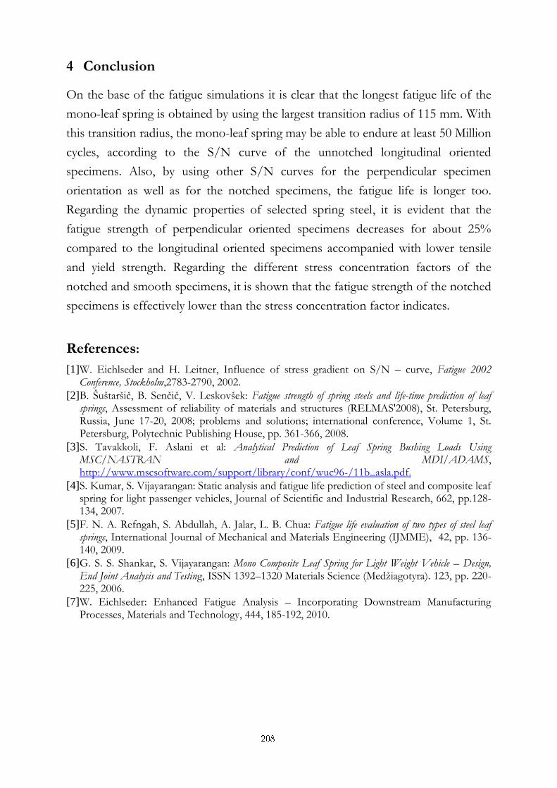
4 Conclusion
On the base of the fatigue simulations it is clear that the longest fatigue life of the
mono-leaf spring is obtained by using the largest transition radius of 115 mm. With
this transition radius, the mono-leaf spring may be able to endure at least 50 Million
cycles, according to the S/N curve of the unnotched longitudinal oriented
specimens. Also, by using other S/N curves for the perpendicular specimen
orientation as well as for the notched specimens, the fatigue life is longer too.
Regarding the dynamic properties of selected spring steel, it is evident that the
fatigue strength of perpendicular oriented specimens decreases for about 25%
compared to the longitudinal oriented specimens accompanied with lower tensile
and yield strength. Regarding the different stress concentration factors of the
notched and smooth specimens, it is shown that the fatigue strength of the notched
specimens is effectively lower than the stress concentration factor indicates.
References:
[1] W. Eichlseder and H. Leitner, Influence of stress gradient on S/N – curve, Fatigue 2002 Conference, Stockholm,2783-2790, 2002.
[2] B. Šuštaršič, B. Senčič, V. Leskovšek: Fatigue strength of spring steels and life-time prediction of leaf springs, Assessment of reliability of materials and structures (RELMAS'2008), St. Petersburg, Russia, June 17-20, 2008; problems and solutions; international conference, Volume 1, St. Petersburg, Polytechnic Publishing House, pp. 361-366, 2008.
[3] S. Tavakkoli, F. Aslani et al: Analytical Prediction of Leaf Spring Bushing Loads Using MSC/NASTRAN and MDI/ADAMS, http://www.mscsoftware.com/support/library/conf/wuc96-/11b_asla.pdf.
[4] S. Kumar, S. Vijayarangan: Static analysis and fatigue life prediction of steel and composite leaf spring for light passenger vehicles, Journal of Scientific and Industrial Research, 662, pp.128-134, 2007.
[5] F. N. A. Refngah, S. Abdullah, A. Jalar, L. B. Chua: Fatigue life evaluation of two types of steel leaf springs, International Journal of Mechanical and Materials Engineering (IJMME), 42, pp. 136-140, 2009.
[6] G. S. S. Shankar, S. Vijayarangan: Mono Composite Leaf Spring for Light Weight Vehicle – Design, End Joint Analysis and Testing, ISSN 1392–1320 Materials Science (Medžiagotyra). 123, pp. 220-225, 2006.
[7] W. Eichlseder: Enhanced Fatigue Analysis – Incorporating Downstream Manufacturing Processes, Materials and Technology, 444, 185-192, 2010.
208

For wider interest
One of the largest European producers of the spring steel material is Štore Steel
Plant, which produces material for truck springs and the other springs for
automotive applications. Generally, spring manufacturers produce springs from
steel in the as-delivered condition. The springs are then heat-treated and tested.
However, the fatigue testing of springs after manufacturing is a time-consuming
and an expensive task. It is also too late to provide information to the steel
producer, who needs in-time and appropriate information about the quality of the
steel in the production from batch to batch. The aim of this research work is to
develop a model which will enable the assessment of the fatigue life of mono and
double leaf-spring based on information of material properties in the as-delivered
condition. The idea is to model both mono and double-leaf spring and then run the
simulations and determine the lifetime of the leaf springs. For our project, we use
their spring steel in the as-delivered condition to perform dynamic tests on
specimens, in order to obtain the material properties, which are the base for the
leaf spring simulation. Since the spring steel manufacturer, as well as the spring
producer, need fast data about the quality of their products, the idea is to use a
faster testing machine for evaluating base material properties.
209
Tailoring electrically-induced properties by stretching relaxor polymer films
G. Casar1,2, A. Eršte1,2, S. Glinšek1,2, X. Li3, X. Qian3, Q. M. Zhang3 and
V. Bobnar1,2
1 Jožef Stefan Institute, Ljubljana, Slovenia
2 Jožef Stefan International Postgraduate School, Ljubljana, Slovenia
3 Department of Electrical Engineering and Materials Research Institute, The Pennsylvania State University, University Park, Pennsylvania 16802, USA
Abstract. Electrically-induced behaviuor was compared in the non-stretched
and uniaxially stretched poly(vinylidene fluoride-trifluoroethylene-
chlorofluoroethylene) terpolymer - a member of the relaxor polymer family
that exhibits fast response speeds, a giant electrostriction, high electric energy
density and a large electrocaloric effect. Although the temperature dependence
of the low-field dielectric constant is almost identical, the dc bias electric field
via a higher nonlinear contribution more heavily alters the dielectric response
of the less-oriented non-stretched samples. Substantial differences in the
polarization, electrocaloric response and induced electrostrictive strain of the
non-stretched and stretched terpolymer suggest that electrically-induced
properties of relaxor polymer films can be tailored by controlling the
preparation conditions.
Keywords: relaxor, polymer, dielectric spectroscopy
Relaxor polymers are of great interest for various advanced applications because of
their giant dielectric, electromechanical and electrocaloric response. We have
investigated and compared these electrically-induced responses in the non-stretched
and uniaxially stretched poly(vinylidene fluoride-trifluoroethylene-chloro-
fluoroethylene), P(VDF-TrFE-CFE), relaxor terpolymer. It is namely known that
stretching of polymer films strongly affects their microstructure, i.e., the
conformation of polymer chains for example, a ferroelectric poly(vinylidene
fluoride) spontaneously crystallizes into a nonpolar trans-gauche chain
conformation, which is transformed into a ferroelectric all-trans conformation only
210
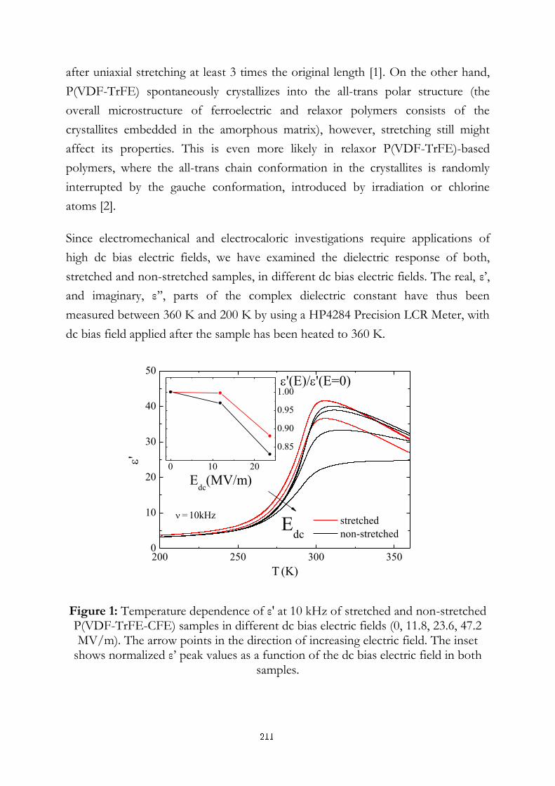
after uniaxial stretching at least 3 times the original length [1]. On the other hand,
P(VDF-TrFE) spontaneously crystallizes into the all-trans polar structure (the
overall microstructure of ferroelectric and relaxor polymers consists of the
crystallites embedded in the amorphous matrix), however, stretching still might
affect its properties. This is even more likely in relaxor P(VDF-TrFE)-based
polymers, where the all-trans chain conformation in the crystallites is randomly
interrupted by the gauche conformation, introduced by irradiation or chlorine
atoms [2].
Since electromechanical and electrocaloric investigations require applications of
high dc bias electric fields, we have examined the dielectric response of both,
stretched and non-stretched samples, in different dc bias electric fields. The real, ε’,
and imaginary, ε’’, parts of the complex dielectric constant have thus been
measured between 360 K and 200 K by using a HP4284 Precision LCR Meter, with
dc bias field applied after the sample has been heated to 360 K.
0 10 20
0.85
0.90
0.95
1.00'(E)/'(E=0)
Edc
(MV/m)
200 250 300 3500
10
20
30
40
50
stretched
non-stretchedE
dc
'
T (K)
=
10kHz
Figure 1: Temperature dependence of ε' at 10 kHz of stretched and non-stretched P(VDF-TrFE-CFE) samples in different dc bias electric fields (0, 11.8, 23.6, 47.2 MV/m). The arrow points in the direction of increasing electric field. The inset
shows normalized ε’ peak values as a function of the dc bias electric field in both samples.
211
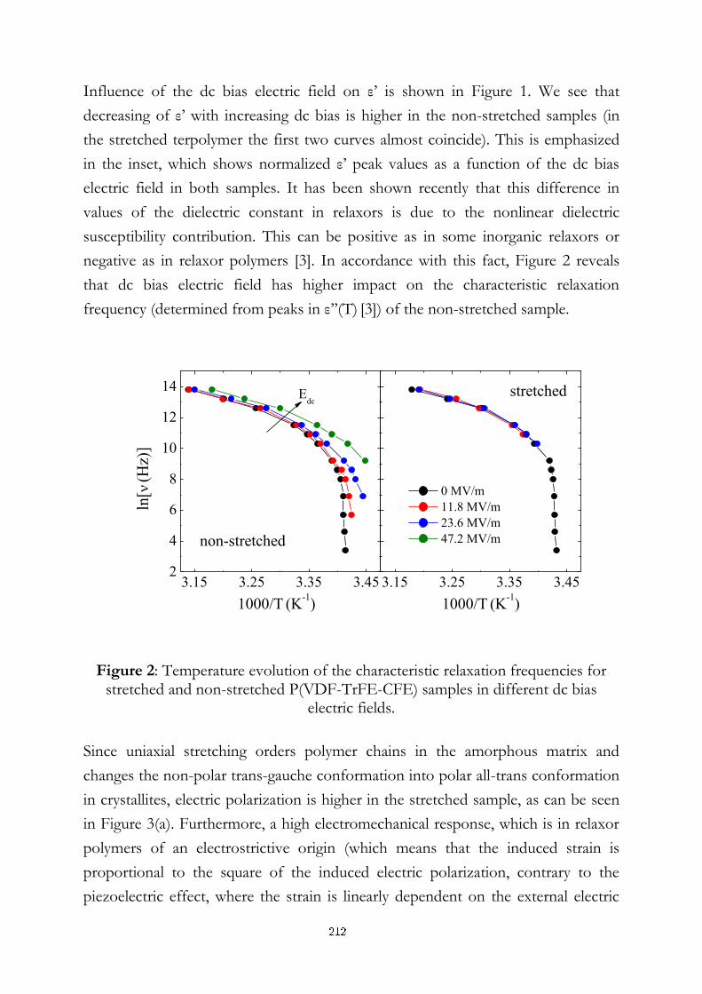
Influence of the dc bias electric field on ε’ is shown in Figure 1. We see that
decreasing of ε’ with increasing dc bias is higher in the non-stretched samples (in
the stretched terpolymer the first two curves almost coincide). This is emphasized
in the inset, which shows normalized ε’ peak values as a function of the dc bias
electric field in both samples. It has been shown recently that this difference in
values of the dielectric constant in relaxors is due to the nonlinear dielectric
susceptibility contribution. This can be positive as in some inorganic relaxors or
negative as in relaxor polymers [3]. In accordance with this fact, Figure 2 reveals
that dc bias electric field has higher impact on the characteristic relaxation
frequency (determined from peaks in ε’’(T) [3]) of the non-stretched sample.
3.15 3.25 3.35 3.452
4
6
8
10
12
14
3.15 3.25 3.35 3.45
Edc
0 MV/m
11.8 MV/m
23.6 MV/m
47.2 MV/m
1000/T (K
-1)
ln[
(Hz)
]
non-stretched
stretched
1000/T (K
-1)
Figure 2: Temperature evolution of the characteristic relaxation frequencies for stretched and non-stretched P(VDF-TrFE-CFE) samples in different dc bias
electric fields.
Since uniaxial stretching orders polymer chains in the amorphous matrix and
changes the non-polar trans-gauche conformation into polar all-trans conformation
in crystallites, electric polarization is higher in the stretched sample, as can be seen
in Figure 3(a). Furthermore, a high electromechanical response, which is in relaxor
polymers of an electrostrictive origin (which means that the induced strain is
proportional to the square of the induced electric polarization, contrary to the
piezoelectric effect, where the strain is linearly dependent on the external electric
212
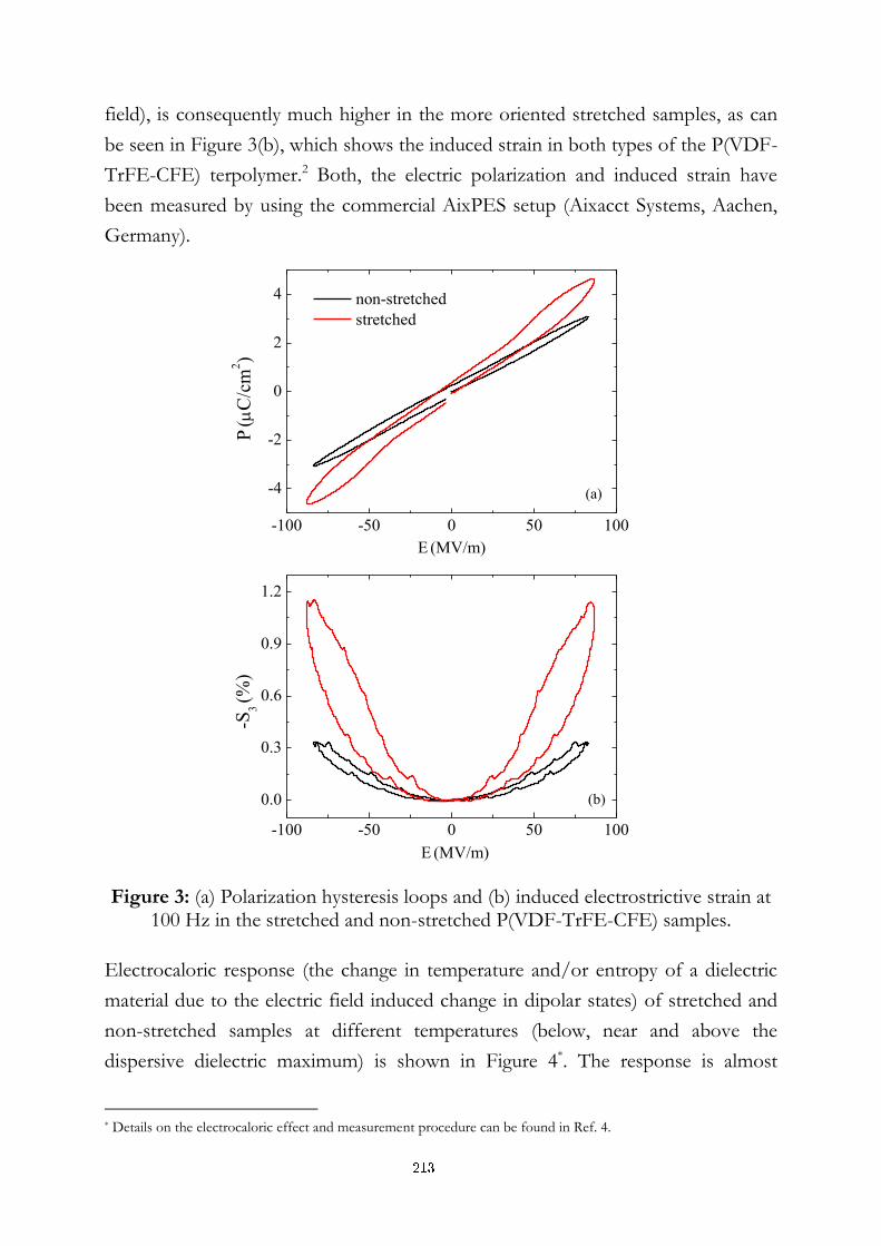
field), is consequently much higher in the more oriented stretched samples, as can
be seen in Figure 3(b), which shows the induced strain in both types of the P(VDF-
TrFE-CFE) terpolymer.2 Both, the electric polarization and induced strain have
been measured by using the commercial AixPES setup (Aixacct Systems, Aachen,
Germany).
-100 -50 0 50 100
-4
-2
0
2
4
-100 -50 0 50 100
0.0
0.3
0.6
0.9
1.2
non-stretched
stretched
P
(C
/cm
2)
E (MV/m)
(a)
(b)
-S3
(%)
E (MV/m)
Figure 3: (a) Polarization hysteresis loops and (b) induced electrostrictive strain at 100 Hz in the stretched and non-stretched P(VDF-TrFE-CFE) samples.
Electrocaloric response (the change in temperature and/or entropy of a dielectric
material due to the electric field induced change in dipolar states) of stretched and
non-stretched samples at different temperatures (below, near and above the
dispersive dielectric maximum) is shown in Figure 4*. The response is almost
* Details on the electrocaloric effect and measurement procedure can be found in Ref. 4.
213
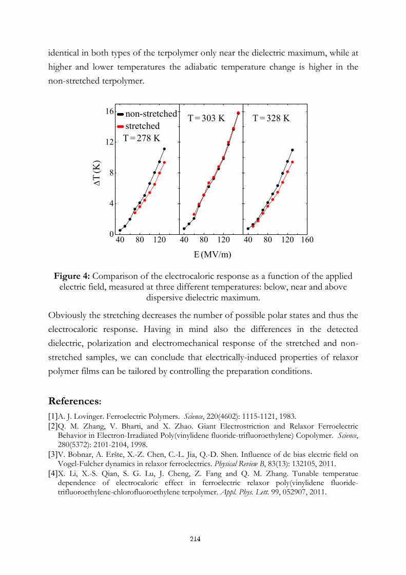
identical in both types of the terpolymer only near the dielectric maximum, while at
higher and lower temperatures the adiabatic temperature change is higher in the
non-stretched terpolymer.
40 80 1200
4
8
12
16
40 80 120 40 80 120 160
T (K
)
E (MV/m)
non-stretched
stretched
T =
278 K
T =
303 K
T =
328 K
Figure 4: Comparison of the electrocaloric response as a function of the applied electric field, measured at three different temperatures: below, near and above
dispersive dielectric maximum.
Obviously the stretching decreases the number of possible polar states and thus the
electrocaloric response. Having in mind also the differences in the detected
dielectric, polarization and electromechanical response of the stretched and non-
stretched samples, we can conclude that electrically-induced properties of relaxor
polymer films can be tailored by controlling the preparation conditions.
References:
[1] A. J. Lovinger. Ferroelectric Polymers. Science, 220(4602): 1115-1121, 1983.
[2] Q. M. Zhang, V. Bharti, and X. Zhao. Giant Electrostriction and Relaxor Ferroelectric Behavior in Electron-Irradiated Poly(vinylidene fluoride-trifluoroethylene) Copolymer. Science, 280(5372): 2101-2104, 1998.
[3] V. Bobnar, A. Eršte, X.-Z. Chen, C.-L. Jia, Q.-D. Shen. Influence of dc bias electric field on Vogel-Fulcher dynamics in relaxor ferroelectrics. Physical Review B, 83(13): 132105, 2011.
[4] X. Li, X.-S. Qian, S. G. Lu, J. Cheng, Z. Fang and Q. M. Zhang. Tunable temperatue dependence of electrocaloric effect in ferroelectric relaxor poly(vinylidene fluoride-trifluoroethylene-chlorofluoroethylene terpolymer. Appl. Phys. Lett. 99, 052907, 2011.
214
For wider interest
Dielectric spectroscopy investigates electrically-induced properties of a material as a
function of frequency and/or temperature. Dielectric properties are related to
polarizability and thus depend on the structure and molecular properties of a
material. That is why dielectric spectroscopy is a useful tool for material
characterization and it is used in pharmacy, biotechnology and material science.
The basic quantity in dielectric spectroscopy is complex dielectric constant ε*,
which consists of the real, ε’, and imaginary, ε’’, part. The real part is related to the
stored energy within the medium, whereas the imaginary part describes the losses.
That is why the dielectric constant is very important in devices for storing electrical
energy (capacitors).
Besides storing electrical energy, there are also materials that are able to convert it
into mechanical work (electromechanical effect) or into heat (electrocaloric effect)
note that electrical energy converted into heat in electrocalorics is not due to the
electrical current running through them. Such properties of a material can be
utilized in many devices such as actuators, sonars, integrated
microelectromechanical systems or artificial muscles, which use the
electromechanical effect, or in heating/cooling devices of new generation, which
use the electrocaloric effect.
Example of materials that possess giant electromechanical and electrocaloric effect
are relaxors and ferroelectrics. Our subject of study was special class of relaxors –
relaxor polymers. Relaxor polymers in comparison to the other inorganic relaxors
have some advantages: they have greater electromechanical response, exhibit fast
response speeds and can also be prepared in a variety of shapes. Their disadvantage
would be that they are stable only at relatively low temperatures (below 100 °C).
Dielectric constant is important for the electromechanical application of relaxor
polymers, since the input electrical energy that can be converted into the strain
energy, is directly proportional to the values of the dielectric constant of the
material. Thus, in order to achieve better efficiency, systems with high values of the
dielectric constant must be developed.
215
Terpolymer/copolymer blends on aluminum surface: Structural, caloric, and dielectric properties
Andreja Eršte1,2, Vid Bobnar1,2, Xian-Zhong Chen3, Cheng-Liang Jia3,
Qun-Dong Shen3
1 Condensed Matter Physics Department, Jožef Stefan Institute, Ljubljana, Slovenia
2 Jožef Stefan International Postgraduate School, Ljubljana, Slovenia
3 Department of Polymer Science and Engineering and Key Laboratory of
Mesoscopic Chemistry of MOE, School of Chemistry and Chemical Engineering,
Nanjing University, Nanjing, China
[email protected] (email of corresponding author)
Abstract. We report structural, caloric, and dielectric properties of polymer
blends of poly(vinylidenefluoride–trifluoroethylene–chlorofluoroethylene)
terpolymer (a member of the relaxor polymers family that exhibits fast
response speeds, giant electrostriction, high electric energy density, and large
electrocaloric effect) and poly(vinylidenefluoride–chlorotrifluoroethylene)
copolymer, developed on aluminium surface. Terpolymer films exhibit for a
relaxor polymer very high values of the dielectric constant of ≈80 around
room temperature, which decreases in terpolymer/copolymer blends to ≈60.
This arises not only from the interference effect but also from the fact that
copolymer additive disturbs the crystallizing process, as being revealed by X–
ray diffraction and differential scanning calorimetry experiments. We show
that addition of the copolymer enables us to govern the value of the dielectric
constant of the films without influencing the relaxor dielectric dynamics.
Keywords: relaxor, polymer, blend, film on surface, dielectric spectroscopy
Relaxor polymers are very promising for a broad range of energy storage capacitor
applications due to their unique physical properties. One of the advantages for use
of polymers in such applications arises from the possibility of polymer film
formation directly on a surface. Active metals such as aluminum can be used for
substrates, as they are less expensive than noble metals and mechanically more
stable than glassy carbon.
216
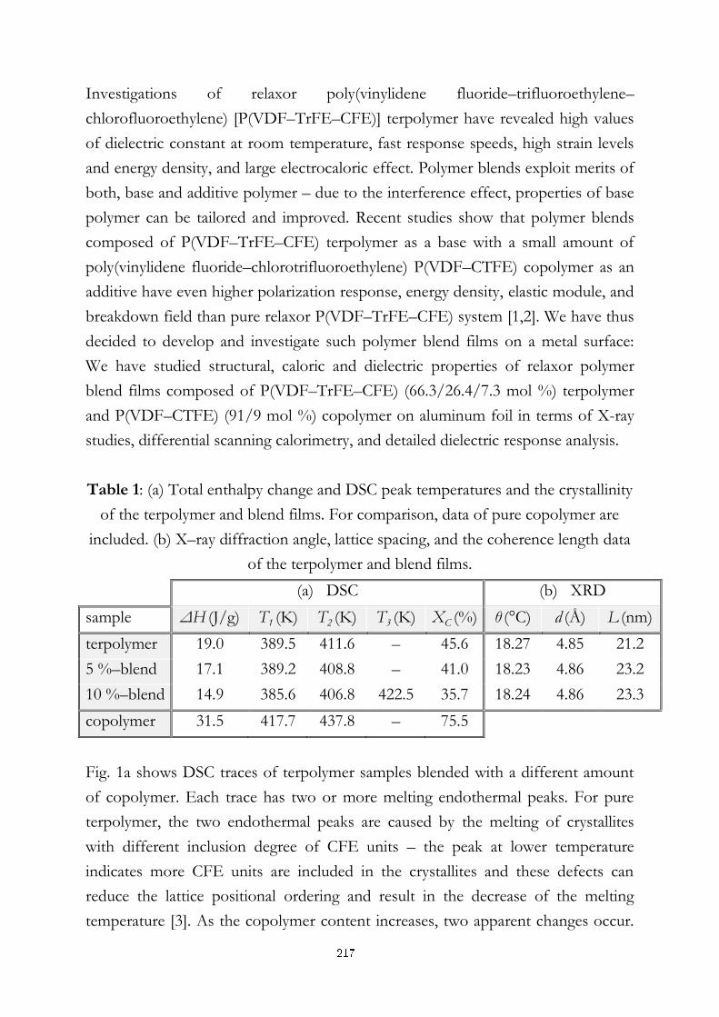
Investigations of relaxor poly(vinylidene fluoride–trifluoroethylene–
chlorofluoroethylene) [P(VDF–TrFE–CFE)] terpolymer have revealed high values
of dielectric constant at room temperature, fast response speeds, high strain levels
and energy density, and large electrocaloric effect. Polymer blends exploit merits of
both, base and additive polymer – due to the interference effect, properties of base
polymer can be tailored and improved. Recent studies show that polymer blends
composed of P(VDF–TrFE–CFE) terpolymer as a base with a small amount of
poly(vinylidene fluoride–chlorotrifluoroethylene) P(VDF–CTFE) copolymer as an
additive have even higher polarization response, energy density, elastic module, and
breakdown field than pure relaxor P(VDF–TrFE–CFE) system [1,2]. We have thus
decided to develop and investigate such polymer blend films on a metal surface:
We have studied structural, caloric and dielectric properties of relaxor polymer
blend films composed of P(VDF–TrFE–CFE) (66.3/26.4/7.3 mol %) terpolymer
and P(VDF–CTFE) (91/9 mol %) copolymer on aluminum foil in terms of X-ray
studies, differential scanning calorimetry, and detailed dielectric response analysis.
Table 1: (a) Total enthalpy change and DSC peak temperatures and the crystallinity
of the terpolymer and blend films. For comparison, data of pure copolymer are
included. (b) X–ray diffraction angle, lattice spacing, and the coherence length data
of the terpolymer and blend films.
(a) DSC (b) XRD
sample ΔH (J/g) T1 (K) T2 (K) T3 (K) XC (%) θ (°C) d (Å) L (nm)
terpolymer 19.0 389.5 411.6 – 45.6 18.27 4.85 21.2
5 %–blend 17.1 389.2 408.8 – 41.0 18.23 4.86 23.2
10 %–blend 14.9 385.6 406.8 422.5 35.7 18.24 4.86 23.3
copolymer 31.5 417.7 437.8 – 75.5
Fig. 1a shows DSC traces of terpolymer samples blended with a different amount
of copolymer. Each trace has two or more melting endothermal peaks. For pure
terpolymer, the two endothermal peaks are caused by the melting of crystallites
with different inclusion degree of CFE units – the peak at lower temperature
indicates more CFE units are included in the crystallites and these defects can
reduce the lattice positional ordering and result in the decrease of the melting
temperature [3]. As the copolymer content increases, two apparent changes occur.
217
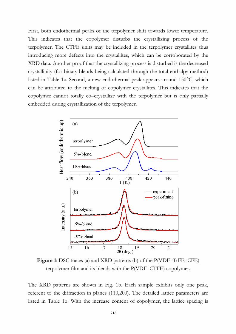
First, both endothermal peaks of the terpolymer shift towards lower temperature.
This indicates that the copolymer disturbs the crystallizing process of the
terpolymer. The CTFE units may be included in the terpolymer crystallites thus
introducing more defects into the crystallites, which can be corroborated by the
XRD data. Another proof that the crystallizing process is disturbed is the decreased
crystallinity (for binary blends being calculated through the total enthalpy method)
listed in Table 1a. Second, a new endothermal peak appears around 150°C, which
can be attributed to the melting of copolymer crystallites. This indicates that the
copolymer cannot totally co–crystallize with the terpolymer but is only partially
embedded during crystallization of the terpolymer.
Figure 1: DSC traces (a) and XRD patterns (b) of the P(VDF–TrFE–CFE)
terpolymer film and its blends with the P(VDF–CTFE) copolymer.
The XRD patterns are shown in Fig. 1b. Each sample exhibits only one peak,
referent to the diffraction in planes (110,200). The detailed lattice parameters are
listed in Table 1b. With the increase content of copolymer, the lattice spacing is
(a)
(b)
218
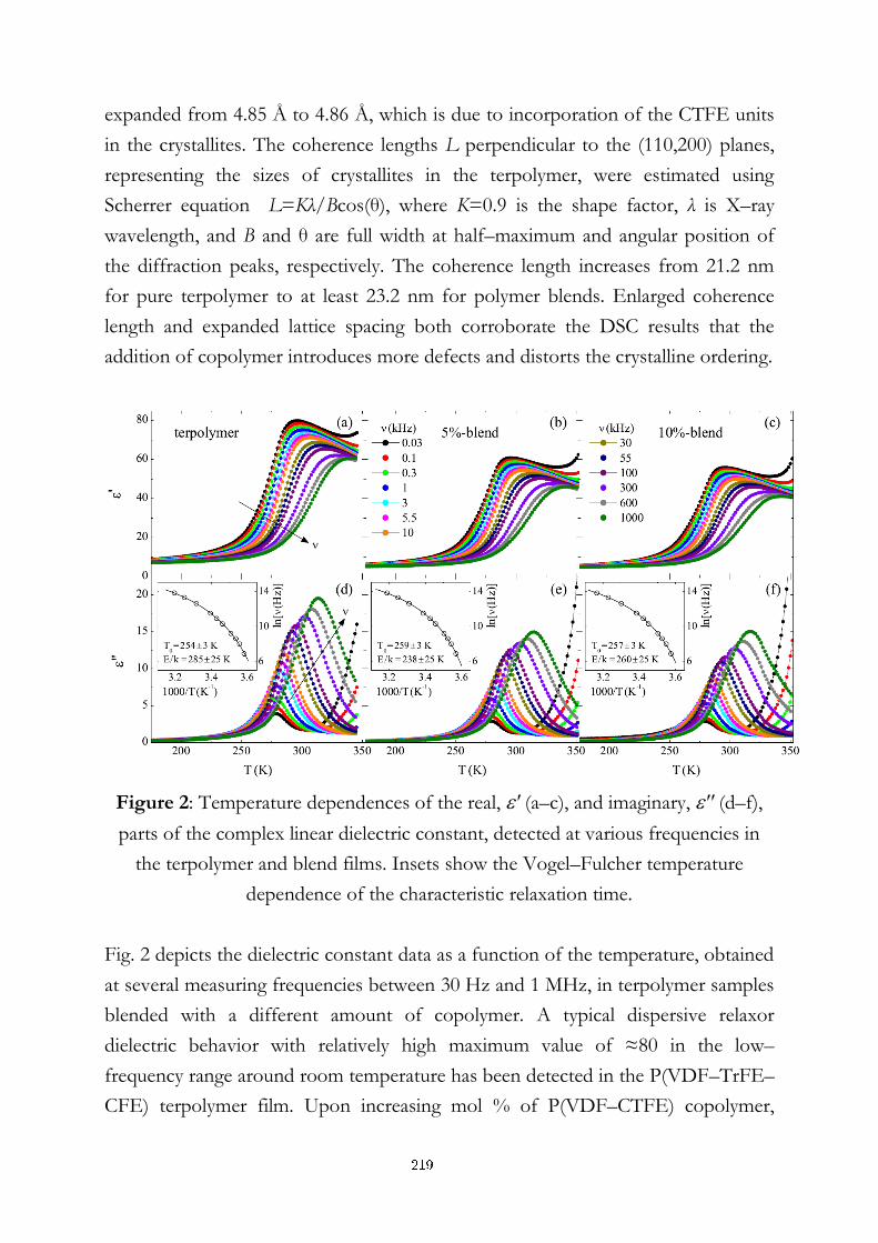
expanded from 4.85 Å to 4.86 Å, which is due to incorporation of the CTFE units
in the crystallites. The coherence lengths L perpendicular to the (110,200) planes,
representing the sizes of crystallites in the terpolymer, were estimated using
Scherrer equation L=Kλ/Bcos(θ), where K=0.9 is the shape factor, λ is X–ray
wavelength, and B and θ are full width at half–maximum and angular position of
the diffraction peaks, respectively. The coherence length increases from 21.2 nm
for pure terpolymer to at least 23.2 nm for polymer blends. Enlarged coherence
length and expanded lattice spacing both corroborate the DSC results that the
addition of copolymer introduces more defects and distorts the crystalline ordering.
Figure 2: Temperature dependences of the real, ' (a–c), and imaginary, '' (d–f),
parts of the complex linear dielectric constant, detected at various frequencies in
the terpolymer and blend films. Insets show the Vogel–Fulcher temperature
dependence of the characteristic relaxation time.
Fig. 2 depicts the dielectric constant data as a function of the temperature, obtained
at several measuring frequencies between 30 Hz and 1 MHz, in terpolymer samples
blended with a different amount of copolymer. A typical dispersive relaxor
dielectric behavior with relatively high maximum value of ≈80 in the low–
frequency range around room temperature has been detected in the P(VDF–TrFE–
CFE) terpolymer film. Upon increasing mol % of P(VDF–CTFE) copolymer,
219
values of both, ' and '', decrease. This is in concurrence with interference effect
because the values of dielectric constant are lower in copolymer with respect to
terpolymer [1]. Insets to Figs. 2d–f show that characteristic relaxation frequencies,
determined from peaks in ''(T), follow the Vogel–Fulcher law (as being typical for
relaxor systems [4]) =0 exp[-E/k(T–T0)], where 0 is the inverse attempt
frequency, E/k is the activation energy (in which k is the Boltzmann constant), and
T0 is the Vogel–Fulcher freezing temperature. No notable differences within
statistical error in Vogel–Fulcher temperature and activation energy between
terpolymer and terpolymer/copolymer blends have been detected, indicating that
the level of crystallization has no influence on the relaxor dielectric dynamics of the
terpolymer film.
In summary, we have investigated structural, caloric, and dielectric properties of
relaxor polymer blend films composed of P(VDF–TrFE–CFE) (66.3/26.4/7.3 mol
%) terpolymer and P(VDF–CTFE) (91/9 mol %) copolymer on aluminum foil.
DSC and XRD results indicate that in this system, the copolymer additive disturbs
the crystallizing process of the terpolymer. Measurements of temperature–
dependent dielectric response revealed that upon increasing mol % of the
copolymer, values of both, ' and '', decrease in comparison to pure terpolymer,
which is in concurrence with interference effect (as values of dielectric constant are
lower in pure copolymer). Analysis of temperature–dependent dielectric response
has revealed that the addition of the copolymer does not influence the relaxor
dynamics of the system: There are no notable differences within statistical error
between Vogel–Fulcher temperatures and activation energies of terpolymer and
blends with 5 or 10 mol % of copolymer.
References:
[1] B. Chu, B, Neese, M, Lin, S-G Lu, and Q. M. Zhang. Enhancement of dielectric energy density in the poly(vinylidene fluoride)-based terpolymer/copolymer blends. Applied Physics Letters, 93(15): 152903, 2008.
[2] B. Neese, B. Chu, S-G Lu, Y. Wang, E. Furman, and Q. M. Zhang. Large electrocaloric effect in ferroelectric polymers near room temperature. Science, 321(5890): 821-823, 2008.
[3] R. J. Klein, J. Runt, and Q. M. Zhang. Influence of crystallization conditions on the microstructure and electromechanical properties of poly(vinylidene fluoride-trifluoroethylene-chlorofluoroethylene) terpolymers. Macromolecules, 36(19): 7220-7226, 2003.
[4] V. Bobnar, B. Vodopivec, A. Levstik, M. Kosec, B. Hilczer, and Q. M. Zhang. Dielectric properties of relaxor-like vinylidene fluoride−trifluoroethylene-based electroactive polymers. Macromolecules, 36(12): 4436-4442, 2003.
220
For wider interest
Relaxor polymers are very promising for a broad range of energy storage capacitor
applications due to their unique physical properties. One of the advantages for use
of polymers in such applications arises from the possibility of polymer film
formation directly on a surface. Active metals such as aluminum can be used for
substrates, as they are less expensive than noble metals and mechanically more
stable than glassy carbon. .
Investigations of relaxor poly(vinylidene fluoride–trifluoroethylene–
chlorofluoroethylene) [P(VDF–TrFE–CFE)] terpolymer have revealed high values
of dielectric constant at room temperature, fast response speeds, high strain levels
and energy density, and large electrocaloric effect. Polymer blends exploit merits of
both, base and additive polymer – due to interference effect, properties of base
polymer can be tailored and improved. Recent studies show that polymer blends
composed of P(VDF–TrFE–CFE) terpolymer as a base with a small amount of
poly(vinylidene fluoride–chlorotrifluoroethylene) P(VDF–CTFE) copolymer (e.g. 5
or 10 mol %) as an additive have even higher polarization response, energy density,
elastic module, and breakdown field than pure relaxor P(VDF–TrFE–CFE) system.
We have thus decided to develop and investigate such polymer blend films on a
metal surface. .
We report structural, caloric, and dielectric properties of polymer blends of
poly(vinylidenefluoride–trifluoroethylene–chlorofluoroethylene) terpolymer (a
member of the relaxor polymers family that exhibits fast response speeds, giant
electrostriction, high electric energy density, and large electrocaloric effect) and
poly(vinylidenefluoride–chlorotrifluoroethylene) copolymer, developed on
aluminum surface. Terpolymer films exhibit for a relaxor polymer material very
high values of the dielectric constant of ≈80 around room temperature, which
decreases in terpolymer/copolymer blends to ≈60. We show that addition of the
copolymer enables us to govern the dielectric constant of the films without
influencing the relaxor dielectric dynamics.
221
The adhesion of bacteria to austenitic stainless steel (AISI 316L) with different surface finishes
Matej Hočevar1,2, Monika Jenko1, Damjana Drobne3, Sara Novak3
1 Institute of Metals and Technology, Ljubljana, Slovenia
2 Jožef Stefan International Postgraduate School, Ljubljana, Slovenia
3 Department of Biology, Biotechnical Faculty, University of Ljubljana, Ljubljana,
Slovenia
Abstract. Adhesion of bacteria and a biofilm formation on stainless steel is
enhancing the material corrosion and presents a chronic source of the
microbial contamination in food and medical industries. The aim of our
research is to examine the effect of the surface roughness and topography of
austenitic stainless steel (AISI 316L) on the adhesion of bacteria. The surface
morphology of the samples was analysed by the atomic force microscope
(AFM), the contact profilometer, the scanning electron microscope (SEM) and
the contact angle goniometer. Different surface finishes of stainless steel
correspond to different roughness (Ra) values. Escherichia coli (Exb-V1) was
exposed to different surfaces. Based on the literature data, we hypothesized
that the surface roughness and furrows of the similar size as bacteria or
smaller, will affect the bacterial adhesion. So far, it was shown that the
bacteria, for their attachment, prefer cracks and scratches over smooth
surfaces.
Keywords: surface roughness, adhesion, bacteria, stainless steel
1 Introduction
In nature on exposed surfaces microorganisms usually adhere, grow and form
aggregations known as biofilms [1]. The adhesion of bacteria to stainless steel
presents a chronic source of the microbial contamination in food and medical
industries [2], [3]. It also enhances the material corrosion, as well as decreases the
performance of plants, heat exchangers and cooling towers [4], [5], [6].
222
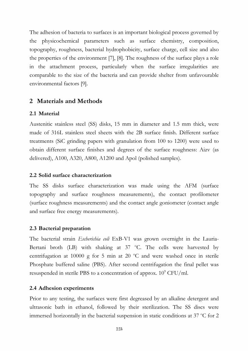
The adhesion of bacteria to surfaces is an important biological process governed by
the physicochemical parameters such as surface chemistry, composition,
topography, roughness, bacterial hydrophobicity, surface charge, cell size and also
the properties of the environment [7], [8]. The roughness of the surface plays a role
in the attachment process, particularly when the surface irregularities are
comparable to the size of the bacteria and can provide shelter from unfavourable
environmental factors [9].
2 Materials and Methods
2.1 Material
Austenitic stainless steel (SS) disks, 15 mm in diameter and 1.5 mm thick, were
made of 316L stainless steel sheets with the 2B surface finish. Different surface
treatments (SiC grinding papers with granulation from 100 to 1200) were used to
obtain different surface finishes and degrees of the surface roughness: Aizv (as
delivered), A100, A320, A800, A1200 and Apol (polished samples).
2.2 Solid surface characterization
The SS disks surface characterization was made using the AFM (surface
topography and surface roughness measurements), the contact profilometer
(surface roughness measurements) and the contact angle goniometer (contact angle
and surface free energy measurements).
2.3 Bacterial preparation
The bacterial strain Escherichia coli ExB-V1 was grown overnight in the Lauria-
Bertani broth (LB) with shaking at 37 oC. The cells were harvested by
centrifugation at 10000 g for 5 min at 20 oC and were washed once in sterile
Phosphate buffered saline (PBS). After second centrifugation the final pellet was
resuspended in sterile PBS to a concentration of approx. 109 CFU/ml.
2.4 Adhesion experiments
Prior to any testing, the surfaces were first degreased by an alkaline detergent and
ultrasonic bath in ethanol, followed by their sterilization. The SS discs were
immersed horizontally in the bacterial suspension in static conditions at 37 oC for 2
223
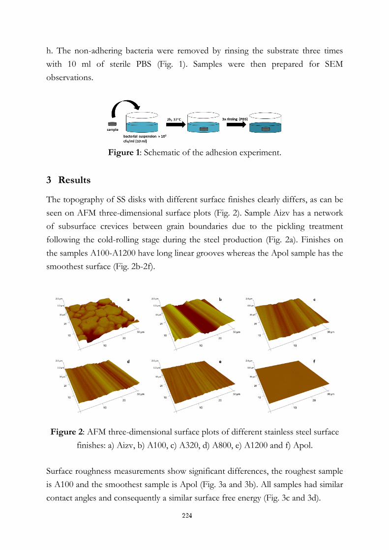
h. The non-adhering bacteria were removed by rinsing the substrate three times
with 10 ml of sterile PBS (Fig. 1). Samples were then prepared for SEM
observations.
Figure 1: Schematic of the adhesion experiment.
3 Results
The topography of SS disks with different surface finishes clearly differs, as can be
seen on AFM three-dimensional surface plots (Fig. 2). Sample Aizv has a network
of subsurface crevices between grain boundaries due to the pickling treatment
following the cold-rolling stage during the steel production (Fig. 2a). Finishes on
the samples A100-A1200 have long linear grooves whereas the Apol sample has the
smoothest surface (Fig. 2b-2f).
Figure 2: AFM three-dimensional surface plots of different stainless steel surface
finishes: a) Aizv, b) A100, c) A320, d) A800, e) A1200 and f) Apol.
Surface roughness measurements show significant differences, the roughest sample
is A100 and the smoothest sample is Apol (Fig. 3a and 3b). All samples had similar
contact angles and consequently a similar surface free energy (Fig. 3c and 3d).
224
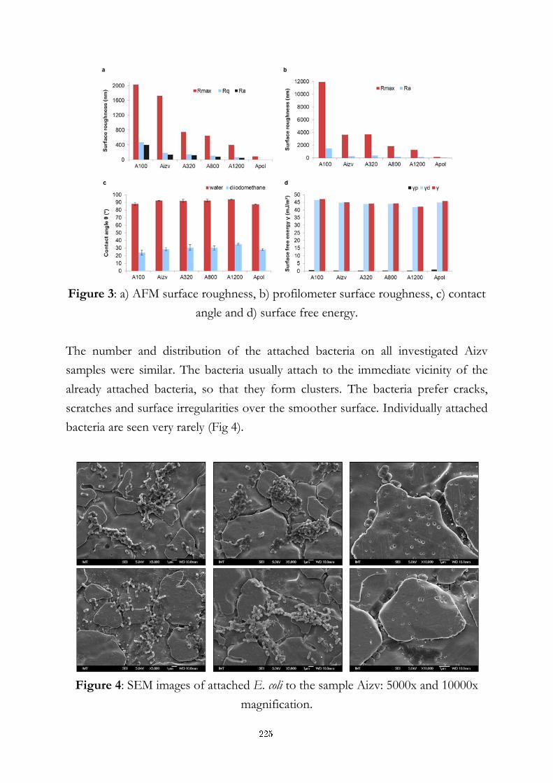
Figure 3: a) AFM surface roughness, b) profilometer surface roughness, c) contact
angle and d) surface free energy.
The number and distribution of the attached bacteria on all investigated Aizv
samples were similar. The bacteria usually attach to the immediate vicinity of the
already attached bacteria, so that they form clusters. The bacteria prefer cracks,
scratches and surface irregularities over the smoother surface. Individually attached
bacteria are seen very rarely (Fig 4).
Figure 4: SEM images of attached E. coli to the sample Aizv: 5000x and 10000x
magnification.
225
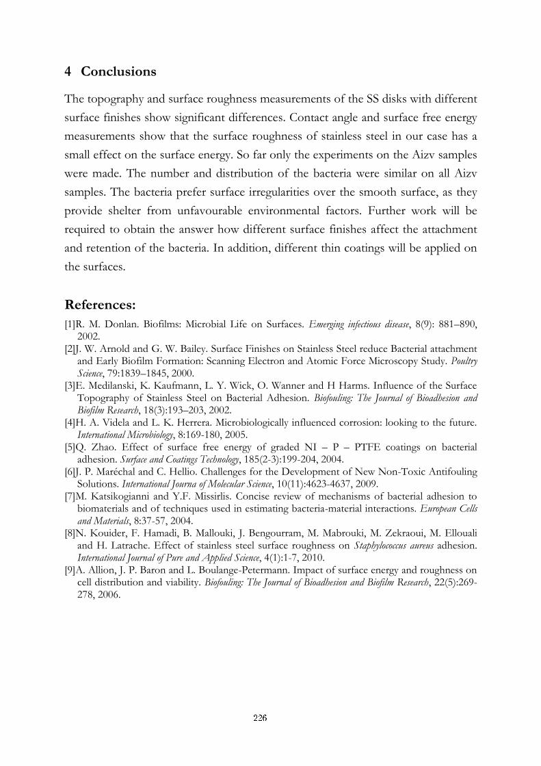
4 Conclusions
The topography and surface roughness measurements of the SS disks with different
surface finishes show significant differences. Contact angle and surface free energy
measurements show that the surface roughness of stainless steel in our case has a
small effect on the surface energy. So far only the experiments on the Aizv samples
were made. The number and distribution of the bacteria were similar on all Aizv
samples. The bacteria prefer surface irregularities over the smooth surface, as they
provide shelter from unfavourable environmental factors. Further work will be
required to obtain the answer how different surface finishes affect the attachment
and retention of the bacteria. In addition, different thin coatings will be applied on
the surfaces.
References:
[1]R. M. Donlan. Biofilms: Microbial Life on Surfaces. Emerging infectious disease, 8(9): 881–890, 2002.
[2]J. W. Arnold and G. W. Bailey. Surface Finishes on Stainless Steel reduce Bacterial attachment and Early Biofilm Formation: Scanning Electron and Atomic Force Microscopy Study. Poultry Science, 79:1839–1845, 2000.
[3]E. Medilanski, K. Kaufmann, L. Y. Wick, O. Wanner and H Harms. Influence of the Surface Topography of Stainless Steel on Bacterial Adhesion. Biofouling: The Journal of Bioadhesion and Biofilm Research, 18(3):193–203, 2002.
[4]H. A. Videla and L. K. Herrera. Microbiologically influenced corrosion: looking to the future. International Microbiology, 8:169-180, 2005.
[5]Q. Zhao. Effect of surface free energy of graded NI – P – PTFE coatings on bacterial adhesion. Surface and Coatings Technology, 185(2-3):199-204, 2004.
[6]J. P. Maréchal and C. Hellio. Challenges for the Development of New Non-Toxic Antifouling Solutions. International Journa of Molecular Science, 10(11):4623-4637, 2009.
[7]M. Katsikogianni and Y.F. Missirlis. Concise review of mechanisms of bacterial adhesion to biomaterials and of techniques used in estimating bacteria-material interactions. European Cells and Materials, 8:37-57, 2004.
[8]N. Kouider, F. Hamadi, B. Mallouki, J. Bengourram, M. Mabrouki, M. Zekraoui, M. Ellouali and H. Latrache. Effect of stainless steel surface roughness on Staphylococcus aureus adhesion. International Journal of Pure and Applied Science, 4(1):1-7, 2010.
[9]A. Allion, J. P. Baron and L. Boulange-Petermann. Impact of surface energy and roughness on cell distribution and viability. Biofouling: The Journal of Bioadhesion and Biofilm Research, 22(5):269-278, 2006.
226
Za širši interes
V naravi mikroorganizmi na izpostavljenih površinah pogosto tvorijo skupke, ki jih
imenujemo biofilmi. Adhezija bakterij na površino in tvorba biofilmov na
nerjavnem jeklu predstavlja kronično vir kontaminacije z mikrobi v medicini in
živilski industriji. Prisotnost bakterij povzroča tudi korozijo materiala ter zmanjšuje
učinkovitost naprav, kot so toplotni izmenjevalci, hladilni stolpi in filtri. Adhezija
bakterij na površino je kompleksen proces na katerega vplivajo lastnosti površine
materiala (hrapavost, topografija, kemija), lastnosti bakterije in okoljski dejavniki.
Namen naše raziskave je preučiti vpliv hrapavosti in topografije nerjavnega jekla na
adhezijo bakterij s pomočjo vrstičnega elektronskega mikroskopa (SEM) in
mikroskopa na atomsko silo (AFM). Za namen naše raziskave smo iz nerjavnega
jekla izdelali vzorce v obliki diskov s premerom 15 mm in debeline 1,5 mm.
Površine vzorcev smo obdelali s pomočjo brusnega papirja različne granulacije
(100-1200), da smo dobili različno topografijo in hrapavost naših vzorcev.
V raziskavi smo uporabili bakterijo Escherichia coli, ki smo jo čez noč gojili v Lauria-
Bertani gojišču s stresanjem pri 37 oC. Nato smo bakterije centrifugirali 5 minut pri
10000 g in dobljeno bakterijsko usedlino resuspendirali v pufru (PBS). Pred
pričetkom adhezijskih poskusov smo vzorce očistili z detergentom, ultrazvočno
kopeljo v absolutnem etanolu in sterilizacijo. Vzorce smo vodoravno potopili v 10
ml bakterijske suspenzije v statičnih pogojih pri 37 °C za 2 h. Nepritrjene oziroma
slabo pritrjene bakterije smo odstranili s tremi zaporednimi spiranji s PBS. Po
adhezijskih poskusih smo vzorce z bakterijami pripravili za mikroskopiranje s SEM.
Do sedaj so bili narejeni poskusi le na vzorcih Aizv. Število in razporeditev bakterij
je pri vseh vzorcih podobna. Bakterije se pritrjajo v neposredno bližino že
pritrjenih bakterij in tvorijo skupke, redkeje je opaziti posamezne bakterije.
Bakterije se pogosteje pritrjujejo v razpoke, praske in druge nepravilnosti na
površini, saj jih ščitijo pred neugodnimi dejavniki okolja. V nadaljevanju naše
raziskave bomo poleg hrapavosti preučevali tudi vpliv tankih plasti na nerjavnem
jeklu na adhezijo bakterij.
227
Influence of the suspension stability on the deposition of
cobalt ferrite particles under an applied magnetic field
Petra Jenuš1,2 , Darja Lisjak1 , Darko Makovec1, Miha Drofenik1,3
1 Department for Materials Synthesis, Jožef Stefan Institute, Ljubljana, Slovenia
2 Jozef Stefan International Postgraduate School, Ljubljana, Slovenia
3 Faculty for Chemistry and Chemical Engineering, Maribor, Slovenia
Abstract. Cobalt ferrite nanoparticles were synthesized with coprecipitation or
with the hydrothermal method. Stable water suspensions were prepared from
the as-synthesized nanoparticles, with the addition of citric acid as a surfactant,
and then used for the preparation of deposits under an applied magnetic field.
The morphology of the cobalt ferrite nanoparticles was investigated with a
transmission electron microscope, and their magnetic properties were
measured with a vibrating-sample magnetometer. The particle sizes and their
magnetic properties influenced the stability of the suspensions, which were
evaluated in terms of their zeta-potentials and the sedimentation time.
Furthermore, the same parameters significantly influenced the morphology of
the deposits, which were observed with a scanning electron microscope.
Keywords: cobalt ferrite, coprecipitation, hydrothermal method,
magneto(di)electric composites
1 Introduction
Cobalt ferrite (CoF), with the chemical formula CoFe2O4, is a spinel ferrite. In
comparison with the other spinel ferrites, CoF has a high cubic magnetocrystalline
anisotropy, a high coercivity and a moderate saturation magnetization [1]. These
interesting magnetic properties, along with a good mechanical hardness, make
cobalt ferrite a promising material for a large number of applications. In addition to
this, CoF is also a magnetostrictive material suitable for magneto(di)electric (ME)
composites [2, 3]. These ME composites are interesting for a variety of
applications, such as tunable microwave devices based on the electric control of the
spin-wave propagation, or new magnetic memories, in which the magnetic
228
response is controlled by an electric field. The magnetostrictive phase in ME
composites can be distributed in a ferroelectric matrix in the form of particles, as
alternating layers or as vertical columnar structures. The latter is denoted as a 1-3
type structure (see also Figure 1d in the following) [4]. It has been shown that the
largest magnetoelectric (ME) effect (the appearance of polarization/magnetization
upon applying a magnetic/electric field) can be produced in the ME composites
with 1-3 structure [5].
Columnar structures can be prepared using a variety of techniques, such as a
pulsed-laser deposition - PLD [6] or a rf sputtering [7]. All these techniques are
quite expensive and complicated. In the search for a simple and inexpensive
method for the preparation of columnar structures, we decided to use the
deposition of CoF nanoparticles under an applied magnetic field. In this work we
investigated how the suspension stability influences the formation of columnar
structures of CoF under an applied magnetic field.
2 Experimental work
Cobalt ferrite nanoparticles were prepared from aqueous solutions of Fe3+ and
Co2+ ions by the coprecipitation (CC) method, where tetramethyl ammonium
hydroxide (TMAH) was used as the precipitating agent and the temperature of the
synthesis was 70°C. CoF nanoparticles were also synthesized by the hydrothermal
(HT) method, where the precipitating agent was sodium hydroxide (NaOH), and
different synthesis temperatures were applied (120°C, 150°C or 200°C). The CoF
nanoparticles were stabilized with citric acid in water, at a pH of approximately 10.
Ten drops of suspension were deposited on an Al2O3 substrate under an applied
magnetic field (B = 0, 5 T) and then dried in the air at room temperature. The
organic phase was removed by heating at 460°C for 2h. The deposition and the
heating procedure were repeated three times.
The CoF nanoparticles were investigated with transmission electron microscopy
(TEM) and with energy-dispersive X-ray spectroscopy (EDXS). The stability of
the suspensions was evaluated from their zeta (potential and the sedimentation
time. This time was determined as the time, before the first sediment of particles
was observed in the suspension. The magnetic properties of the CoF nanopowders
229
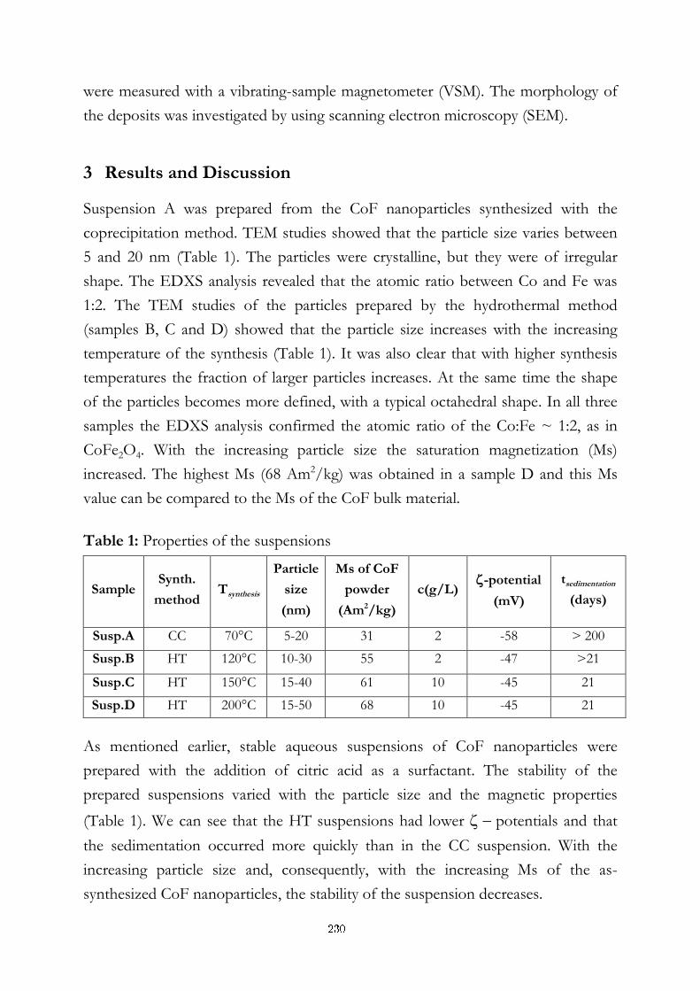
were measured with a vibrating-sample magnetometer (VSM). The morphology of
the deposits was investigated by using scanning electron microscopy (SEM).
3 Results and Discussion
Suspension A was prepared from the CoF nanoparticles synthesized with the
coprecipitation method. TEM studies showed that the particle size varies between
5 and 20 nm (Table 1). The particles were crystalline, but they were of irregular
shape. The EDXS analysis revealed that the atomic ratio between Co and Fe was
1:2. The TEM studies of the particles prepared by the hydrothermal method
(samples B, C and D) showed that the particle size increases with the increasing
temperature of the synthesis (Table 1). It was also clear that with higher synthesis
temperatures the fraction of larger particles increases. At the same time the shape
of the particles becomes more defined, with a typical octahedral shape. In all three
samples the EDXS analysis confirmed the atomic ratio of the Co:Fe ~ 1:2, as in
CoFe2O4. With the increasing particle size the saturation magnetization (Ms)
increased. The highest Ms (68 Am2/kg) was obtained in a sample D and this Ms
value can be compared to the Ms of the CoF bulk material.
Table 1: Properties of the suspensions
Sample Synth.
method Tsynthesis
Particle
size
(nm)
Ms of CoF
powder
(Am2/kg)
c(g/L) -potential
(mV)
tsedimentation
(days)
Susp.A CC 70°C 5-20 31 2 -58 > 200
Susp.B HT 120°C 10-30 55 2 -47 >21
Susp.C HT 150°C 15-40 61 10 -45 21
Susp.D HT 200°C 15-50 68 10 -45 21
As mentioned earlier, stable aqueous suspensions of CoF nanoparticles were
prepared with the addition of citric acid as a surfactant. The stability of the
prepared suspensions varied with the particle size and the magnetic properties
(Table 1). We can see that the HT suspensions had lower potentials and that
the sedimentation occurred more quickly than in the CC suspension. With the
increasing particle size and, consequently, with the increasing Ms of the as-
synthesized CoF nanoparticles, the stability of the suspension decreases.
230
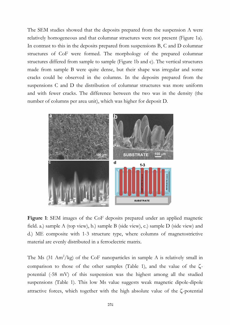
The SEM studies showed that the deposits prepared from the suspension A were
relatively homogeneous and that columnar structures were not present (Figure 1a).
In contrast to this in the deposits prepared from suspensions B, C and D columnar
structures of CoF were formed. The morphology of the prepared columnar
structures differed from sample to sample (Figure 1b and c). The vertical structures
made from sample B were quite dense, but their shape was irregular and some
cracks could be observed in the columns. In the deposits prepared from the
suspensions C and D the distribution of columnar structures was more uniform
and with fewer cracks. The difference between the two was in the density (the
number of columns per area unit), which was higher for deposit D.
Figure 1: SEM images of the CoF deposits prepared under an applied magnetic
field. a.) sample A (top view), b.) sample B (side view), c.) sample D (side view) and
d.) ME composite with 1-3 structure type, where columns of magnetostrictive
material are evenly distributed in a ferroelectric matrix.
The Ms (31 Am2/kg) of the CoF nanoparticles in sample A is relatively small in
comparison to those of the other samples (Table 1), and the value of the -
potential (-58 mV) of this suspension was the highest among all the studied
suspensions (Table 1). This low Ms value suggests weak magnetic dipole-dipole
attractive forces, which together with the high absolute value of the -potential
231
resulted in a very stable suspension. The high degree of stability could also be seen
from the time of the onset of sedimentation, which was longer than 6 months in
case of sample A (Table 1). The CoF nanopowders prepared by the hydrothermal
method had higher values of Ms and, therefore, the attractive magnetic forces
between these CoF particles in the suspension were stronger than in suspension A.
The increasing attractive energy between the particles coincides with the smaller
absolute value of the -potential and, consequently, with the less stable suspension
(see also the sedimentation time in Table 1). All this suggest the suspension stability
affected the deposits’ morphology and that the destabilization of a suspension was
crucial for the formation of the columns.
4 Conclusions
In this work we investigated the influence of the suspension stability on the
deposition of CoF particles under an applied magnetic field. It was shown that the
deposits prepared from a stable suspension were relatively homogenous. From the
suspensions with the lower zeta potential and shorter sedimentation time the
deposits with columnar structures were formed. The columns were distributed
uniformly on a substrate and had smooth surfaces when the deposits were prepared
from the least stable suspensions.
References:
[1] J. Smit, H. P. J. Wijn, Smit, J., Wijn, H. P. J., Ferrites. Eindhoven; Philips' Technical Library, 1959.
[2] H. Zheng, J. Wang, S. E. Lofland, Z. Ma, L. Mohaddes-Ardabili, T. Zhao, L. Salamanca-Riba, S. R. Shinde, S. B. Ogale, F. Bai, D. Viehland, Y. Jia, D. G. Schlom, M. Wuttig, A. Rotyburd, R. Ramesh, Multiferroic BaTiO3 - CoFe2O4 Nanostructures, Science, 303, 661-663, 2004.
[3] J. X. Zhang, J. Y. Dai, W. Lu, H. L. W. Chan, Room Temperature Magnetic Exchange Coupling in Multiferroic BaTiO3 /CoFe2O4 Magnetoelectric Superlattice, J. Mater.Sci, 44, 5142-5148, 2009.
[4] Y. Wang, J. Hu, Y. Lin, C.-W. Nan, Multiferroic Magnetoelectric Composite Nanostructures, NGP Asia Mater., 2(2), 61-68, 2010.
[5] C.-W. Nan, G. Liu, Y. Lin, H. Chen, Magnetic-Field-Induced Electric Polarization in Multiferroic Nanostructures, Phys. Rew. Lett, 94, 197203, 2005.
[6] H. Zheng, J. Wang, L. Mohaddes-Ardabili, M. Wuttig, L. Salamanca-Riba, D. G. Schlom, R. Ramesh, Three-Dimensional Heteroepitaxy in Self-Assembled BaTiO3–CoFe2O4 Nanostructures, Appl. Phys. Lett., 85, 2035-2037, 2004.
[7] I. Fina, N.Dix, V.Laukhin , L.Fabrega , F.Sanchez, J.Fontcuberta, Dielectric Properties of BaTiO3–CoFe2O4 Nanocomposite Thin Films, J. Magn. Magn. Mater., 321, 1795-1798, 2009.
232
For wider interest
Magnetic nanoparticles (magnetic fluids, nanocomposites)
New methods for the controlled synthesis of iron oxide based nanoparticles are
being developed. Additionally, we are focused on the functionalization of magnetic
nanoparticles, primarily for biomedical applications. The surface properties of
nanopowders, which determine their applicability, are tuned with inorganic coatings
(i.e., a thin film of amorphous silica), with polymer coatings or with single-molecule
layers. The coating prevents the agglomeration of nanoparticles, which further
enables their dispersion in various liquids, i.e., magnetic fluids or the homogeneous
incorporation of nanoparticles in various matrices.
Multifunctional materials
Nanocomposites combining the various properties of the constituent materials can
be prepared by mastering the surface properties of nanoparticles. Examples of our
studies include combinations of ferrimagnetics and dielectrics (magnetodielectrics)
and ferrimagnetic and ferroelectric (composite multiferroics) materials. Current
studies are also related to the development of new, magneto-optic materials for
sensors and magneto-catalytic materials for environmental applications.
Magnetic materials for micro- and mm-waves
Magnetic materials suitable for the absorbers of electromagnetic waves and for the
non-reciprocal ferrite devices are being developed. Ceramics and composites based
on ferrites are studied for the microwave applications, and a new method for the
preparation of magnetically oriented thick hexaferrite films for self-biased mm-
wave applications has been developed.
233
Synthesis of cobalt ferrite nanoparticles using a combination of the co-precipitation and hydrothermal methods
Sonja Jovanović1,2, Matjaž Spreitzer1, Mojca Otoničar1,2, Danilo Suvorov1,2
1 Department of Advanced Materials, Jožef Stefan Institute, Ljubljana, Slovenia
2 Jožef Stefan International Postgraduate School, Ljubljana, Slovenia
Abstract. In this work we have examined the influence of the pH on the
structural and magnetic properties of cobalt ferrite (CoFe2O4) nanoparticles
obtained by a combination of the co-precipitation and hydrothermal methods.
The crystal structures and the particle sizes of the prepared powders were
analyzed by the X-ray diffraction and transmission electron microscopy, while
the magnetic properties of the cobalt ferrite nanoparticles were measured at
room temperature using a vibrating-sample magnetometer. The results showed
that an increase of the pH improves both the crystallinity of the CoFe2O4
nanoparticles and their average size. At the same time the pH affects the
magnetic properties of the nanoparticles, since the saturation magnetization
(MS), remanent magnetization (Mr) and coercivity (HC) increase with the
increase of the pH.
Keywords: Cobalt ferrite; Nanoparticles; Hydrothermal synthesis; Magnetic
properties
1 Introduction
The spinel ferrites are a large group of oxides that were first studied by Nishikawa
(1915) and Bragg (1915); they have the structure of the natural spinel MgAl2O4
[1].In recent years, spinel ferrite nanoparticles have been actively investigated
because of their magnetic and electrical properties. The general formula of spinel
ferrites is MFe2O4, where M is a divalent ion such as Co2+, Ni2+, Zn2+, Mn2+, etc.
Cobalt ferrite is a material that possesses an inverse spinel structure. It has a
moderate saturation magnetization, a large magnetic anisotropy, a remarkable
chemical stability and a mechanical hardness, and because of these properties it can
234
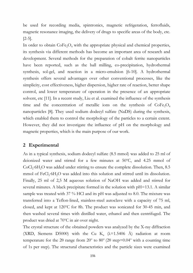
be used for recording media, spintronics, magnetic refrigeration, ferrofluids,
magnetic resonance imaging, the delivery of drugs to specific areas of the body, etc.
[2-5].
In order to obtain CoFe2O4 with the appropriate physical and chemical properties,
its synthesis via different methods has become an important area of research and
development. Several methods for the preparation of cobalt ferrite nanoparticles
have been reported, such as the ball milling, co-precipitation, hydrothermal
synthesis, sol-gel, and reaction in a micro-emulsion [6-10]. A hydrothermal
synthesis offers several advantages over other conventional processes, like the
simplicity, cost effectiveness, higher dispersion, higher rate of reaction, better shape
control, and lower temperature of operation in the presence of an appropriate
solvent, etc [11]. In a recent study, Liu et al. examined the influence of the synthesis
time and the concentration of metallic ions on the synthesis of CoFe2O4
nanoparticles [8]. They used sodium dodecyl sulfate (NaDS) during the synthesis,
which enabled them to control the morphology of the particles to a certain extent.
However, they did not investigate the influence of pH on the morphology and
magnetic properties, which is the main purpose of our work.
2 Experimental
As in a typical synthesis, sodium dodecyl sulfate (8.5 mmol) was added to 25 ml of
deionized water and stirred for a few minutes at 50oC, and 4.25 mmol of
CoCl2∙6H2O was added under stirring to ensure the complete dissolution. Then, 8.5
mmol of FeCl3∙6H2O was added into this solution and stirred until its dissolution.
Finally, 25 ml of 2,5 M aqueous solution of NaOH was added and stirred for
several minutes. A black precipitate formed in the solution with pH=13.1. A similar
sample was treated with 37 % HCl and its pH was adjusted to 8.0. The mixture was
transferred into a Teflon-lined, stainless-steel autoclave with a capacity of 75 ml,
closed, and kept at 120oC for 8h. The product was sonicated for 30-45 min, and
then washed several times with distilled water, ethanol and then centrifuged. The
product was dried at 70oC in air over night.
The crystal structure of the obtained powders was analyzed by the X-ray diffraction
(XRD, Siemens D5000) with the Cu Kα (λ=1.5406 Å) radiation at room
temperature for the 2θ range from 20o to 80o (2θ step=0.04o with a counting time
of 1s per step). The structural characteristics and the particle sizes were examined
235
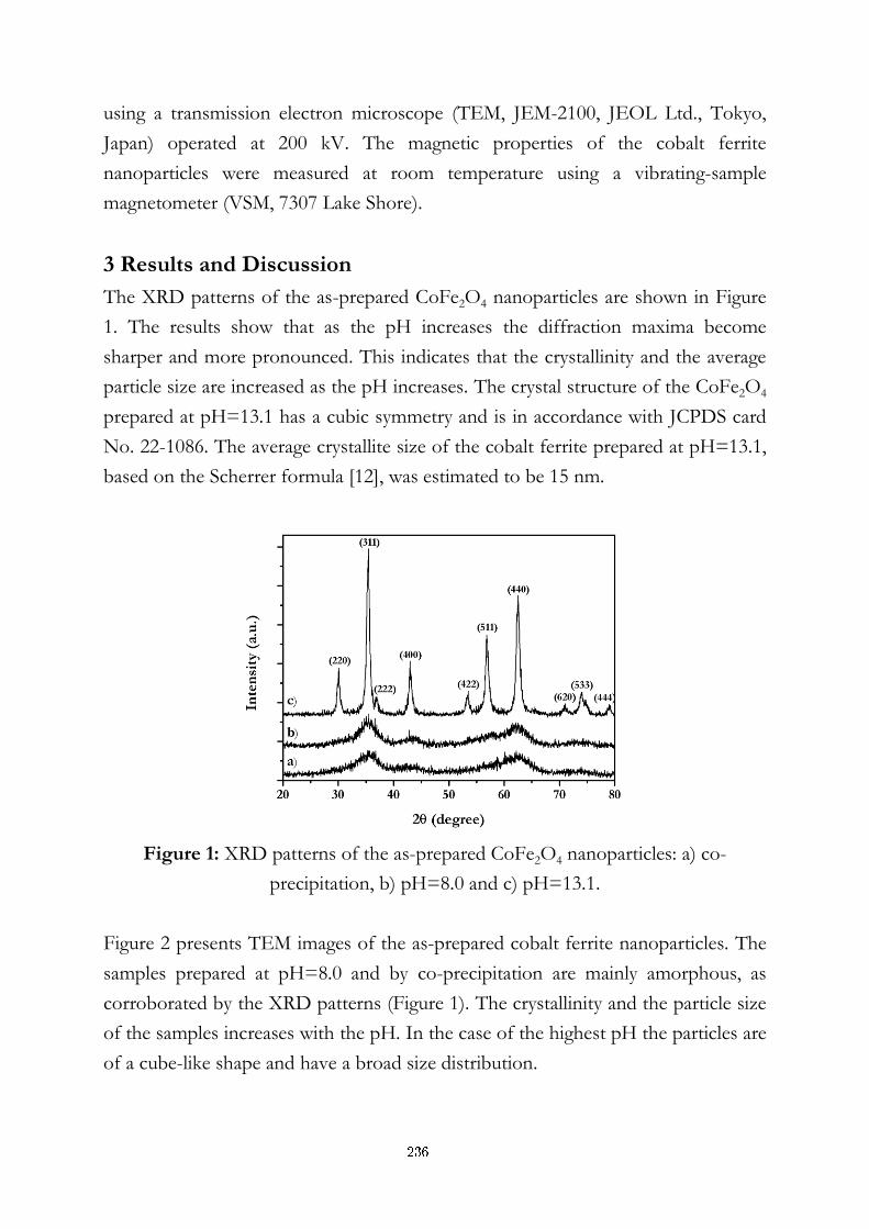
using a transmission electron microscope (TEM, JEM-2100, JEOL Ltd., Tokyo,
Japan) operated at 200 kV. The magnetic properties of the cobalt ferrite
nanoparticles were measured at room temperature using a vibrating-sample
magnetometer (VSM, 7307 Lake Shore).
3 Results and Discussion
The XRD patterns of the as-prepared CoFe2O4 nanoparticles are shown in Figure
1. The results show that as the pH increases the diffraction maxima become
sharper and more pronounced. This indicates that the crystallinity and the average
particle size are increased as the pH increases. The crystal structure of the CoFe2O4
prepared at pH=13.1 has a cubic symmetry and is in accordance with JCPDS card
No. 22-1086. The average crystallite size of the cobalt ferrite prepared at pH=13.1,
based on the Scherrer formula [12], was estimated to be 15 nm.
Figure 1: XRD patterns of the as-prepared CoFe2O4 nanoparticles: a) co-
precipitation, b) pH=8.0 and c) pH=13.1.
Figure 2 presents TEM images of the as-prepared cobalt ferrite nanoparticles. The
samples prepared at pH=8.0 and by co-precipitation are mainly amorphous, as
corroborated by the XRD patterns (Figure 1). The crystallinity and the particle size
of the samples increases with the pH. In the case of the highest pH the particles are
of a cube-like shape and have a broad size distribution.
236
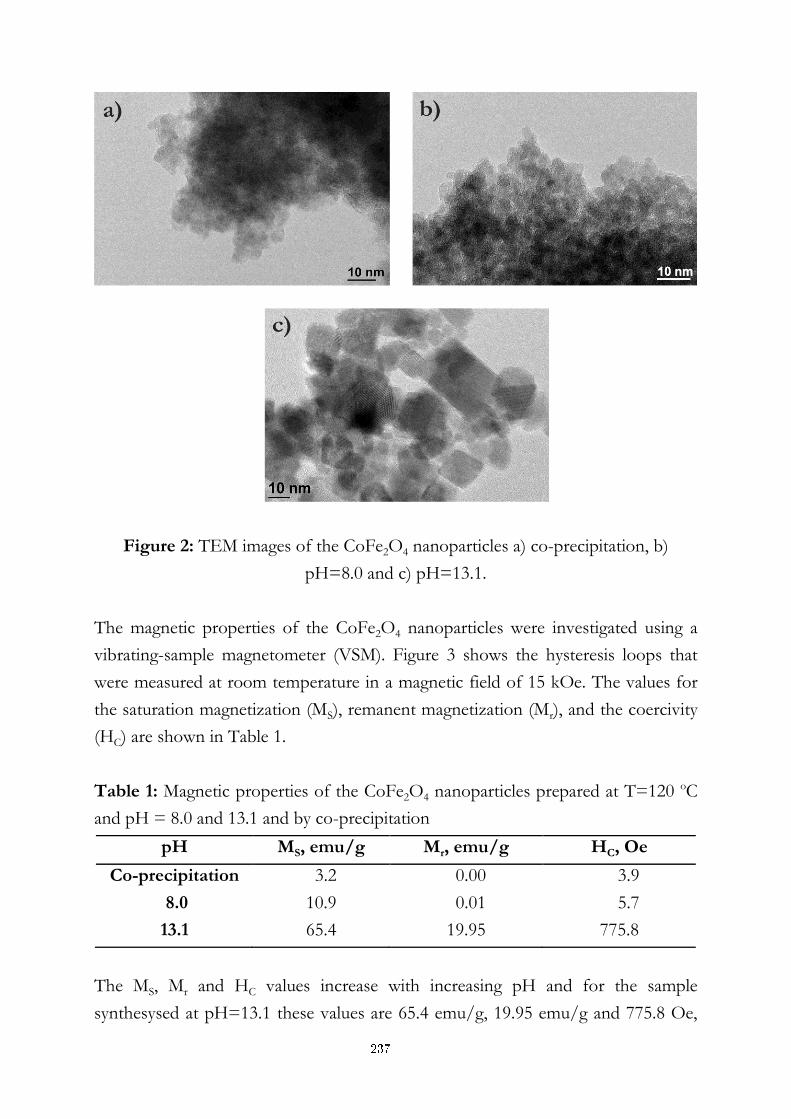
Figure 2: TEM images of the CoFe2O4 nanoparticles a) co-precipitation, b)
pH=8.0 and c) pH=13.1.
The magnetic properties of the CoFe2O4 nanoparticles were investigated using a
vibrating-sample magnetometer (VSM). Figure 3 shows the hysteresis loops that
were measured at room temperature in a magnetic field of 15 kOe. The values for
the saturation magnetization (MS), remanent magnetization (Mr), and the coercivity
(HC) are shown in Table 1.
Table 1: Magnetic properties of the CoFe2O4 nanoparticles prepared at T=120 oC
and pH = 8.0 and 13.1 and by co-precipitation
pH MS, emu/g Mr, emu/g HC, Oe
Co-precipitation 3.2 0.00 3.9
8.0 10.9 0.01 5.7
13.1 65.4 19.95 775.8
The MS, Mr and HC values increase with increasing pH and for the sample
synthesysed at pH=13.1 these values are 65.4 emu/g, 19.95 emu/g and 775.8 Oe,
237
respectively. As is clear from Figure 3, with the increase of the pH the samples
change their magnetic behaviour: they go from paramagnetic to ferromagnetic. We
anticipated that an increase in the magnetic properties is related to the higher
crystallinity of the sample obtained at pH=13.1. Furthermore, we observed that the
values of MS, Mr and HC obtained here (Table 1) are higher than the corresponding
values (60.27 emu/g, 15.63 emu/g and 465 Oe, respectively) reported by Liu at al.
[8].
Figure 3: Hysteresis loops of the CoFe2O4 nanoparticles
4 Conclusion
The effect of pH on the structural and magnetic properties of the CoFe2O4
nanoparticles prepared by a combination of the co-precipitation and hydrothermal
methods was investigated. The results show that the crystallinity and average
particle size increase with the increase of the pH. Also, the values of MS, Mr and HC
follow this trend. The sample prepared at pH=13.1 has the highest values of MS,
Mr and HC (65.4 emu/g, 19.95 emu/g and 775.8 Oe, respectively) and, according to
Scherrer’s equation, the average crystallite size for the sample with pH=13.1 was
estimated to be 15 nm.
References:
[1] Raul Valenzuela. Magnetnic ceramics. Cambridge University Press, 1994.
[2] E. S. Murdock, R. F. Simmons, R. Davidson. Roadmap for 10 Gbit/in2 Media: Challenges. IEEE Transactions on Magnetics, 28 (5): 3078-3083, 1992.
[3] S. N. Okuno, S. Hashimoto, K. lnomata. Preferred crystal orientation of cobalt ferrite thin films induced by ion bombardment during deposition. Journal of Applied Physics, 71 (12): 5926-5929, 1992.
[4] P. C. Rajath Varma, R. S. Manna, D. Banerjee, M. Raama Varma, K. G. Suresh, A. K. Nigam. Magnetic properties of CoFe2O4 synthesized by solid state, citrate precursor and polymerized complex methods: A comparative study. Journal of Alloys and Compounds, 453(1-2): 298-303, 2008.
238

[5] M. Kishimoto, Y. Sakurai, T. Ajima. Magneto‐optical properties of Ba‐ferrite particulate media. Journal of Applied Physics, 76 (11): 7506-7509, 1994.
[6] E. Manova, D. Paneva, B. Kunev, Cl. Estournès, E. Rivière, K. Tenchev, A. Léaustic, I. Mitov. Mechanochemical synthesis and characterization of nanodimnsional iron-cobalt spinel oxides. Journal of Alloys and Compounds, 485 (1-2): 356-361, 2009.
[7] I. Sharifi, H. Shokrollahi, M. M. Doroodmand, R. Safi, Magnetic and structural studies on CoFe2O4 nanoparticles synthesized by co-precipitation, normal micelles and reverse micelles methods, Journal of Magnetism and Magnetic Materials, 324 (10): 1854-1861, 2012.
[8] Q. Liu, J. Sun, H. Long, X. Sun, X. Zhong, Z. Xu. Hydrothermal synthesis of CoFe2O4 nanoplatelets and nanoparticles. Materials Chemistry and Physics, 108 (2-3): 269-273, 2008.
[9] I. H. Gul, A.Maqsood. Structural, magnetic and electrical properties of cobalt ferrites prepared by the sol-gel route. Journal of Alloys and Compounds, 465 (1-2): 227-231, 2008.
[10] V. Pillai, D. O. Shah. Synthesis of high-coercivity cobalt ferrite particles using water-in-oil microemulsions. Journal of Magnetism and Magnetic Materials, 163 (1-2): 243-248, 1996.
[11] M. Yoshimura, K. Burappa. Hydrothermal processing of materials: past, present and future. Journal of Materials Science, 43 (7): 2085-2103, 2008.
[12] Z. Zi, Y. Sun, X. Zhu, Z. Yang, J. Dai, W. Song. Synthesis and magnetic properties of CoFe2O4 ferrite nanoparticles. Journal of Magnetism and Magnetic Materials, 321 (9): 1251-1255, 2009.
239

For wider interest
Because of its magnetic and electrical properties, cobalt ferrite is an interesting
material. It has a moderate saturation magnetization, a large magnetic anisotropy, a
remarkable chemical stability and a mechanical hardness. Because of these
properties it can be used for recording media, spintronics, magnetic refrigeration,
ferrofluids, magnetic resonance imaging, the delivery of drugs to specific areas of
the body, etc. The presented results are part of the project aimed to improve the
magnetic properties of cobalt ferrite particles along with the control of particle
sizes and their stability, which would enhance the applicability of cobalt ferrite.
240
Tempering Effects on the Microstructure, Mechanical Properties and Creep Rate of X20CrMoV121 and P91 Steels
Fevzi Kafexhiu1,2, Franc Vodopivec1, Jelena Vojvodič – Tuma2
1 Department of Surface Engineering and Applied Surface Science, Institute of
Metals and Technology, Ljubljana, Slovenia
2 Jožef Stefan International Postgraduate School, Ljubljana, Slovenia
Abstract. The effect of tempering on the microstructure and room-
temperature yield stress of the two creep-resistant steels, X20CrMoV121 and
P91, was investigated. The samples were tempered for 17520 h at 650 °C and
8760 h at 750 °C. After tempering, the room-temperature yield stress was
determined. In addition, the SEM (Scanning Electron Microscopy) imaging on
the tempered samples was carried out.
It was found that the effect of tempering at 750 °C on the microstructure and
room-temperature yield stress was greater for both steels than the effect of
tempering at 650 °C. Changes of yield stress for both steels were found to be
mutually very similar; hence a general mathematical expression with specific
parameters for both steels and tempering temperatures was deduced. For the
samples tempered at 750 °C only, a fairly good correlation between the inter-
particle spacing, yield stress and creep rate was observed.
Keywords: tempering, microstructure, yield stress, creep rate.
1 Introduction
In recent years there has been an increased demand to raise the efficiency of steam
power plants for economic and environmental reasons. A straight-forward way to
achieve it is to raise the inlet temperature and pressure of the steam that passes the
turbines. This directly saves fuel and reduces CO2 emissions [1].
Issues that arise with higher steam temperatures and pressures are largely material
related, because at such conditions the microstructure changes with time, and as a
result, materials properties change as well. Materials usually employed for power
plants with enhanced steam parameters are the 9-12 % Cr steels [2].
241
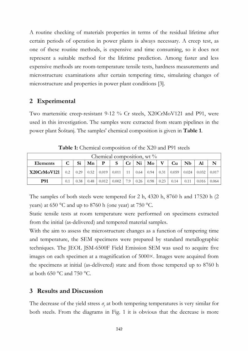
A routine checking of materials properties in terms of the residual lifetime after
certain periods of operation in power plants is always necessary. A creep test, as
one of these routine methods, is expensive and time consuming, so it does not
represent a suitable method for the lifetime prediction. Among faster and less
expensive methods are room-temperature tensile tests, hardness measurements and
microstructure examinations after certain tempering time, simulating changes of
microstructure and properties in power plant conditions [3].
2 Experimental
Two martensitic creep-resistant 9-12 % Cr steels, X20CrMoV121 and P91, were
used in this investigation. The samples were extracted from steam pipelines in the
power plant Šoštanj. The samples' chemical composition is given in Table 1.
Table 1: Chemical composition of the X20 and P91 steels
Chemical composition, wt % Elements C Si Mn P S Cr Ni Mo V Cu Nb Al N
X20CrMoV121 0.2 0.29 0.52 0.019 0.011 11 0.64 0.94 0.31 0.059 0.024 0.032 0.017
P91 0.1 0.38 0.48 0.012 0.002 7.9 0.26 0.98 0.23 0.14 0.11 0.016 0.064
The samples of both steels were tempered for 2 h, 4320 h, 8760 h and 17520 h (2
years) at 650 °C and up to 8760 h (one year) at 750 °C.
Static tensile tests at room temperature were performed on specimens extracted
from the initial (as-delivered) and tempered material samples.
With the aim to assess the microstructure changes as a function of tempering time
and temperature, the SEM specimens were prepared by standard metallographic
techniques. The JEOL JSM-6500F Field Emission SEM was used to acquire five
images on each specimen at a magnification of 5000×. Images were acquired from
the specimens at initial (as-delivered) state and from those tempered up to 8760 h
at both 650 °C and 750 °C.
3 Results and Discussion
The decrease of the yield stress σy at both tempering temperatures is very similar for
both steels. From the diagrams in Fig. 1 it is obvious that the decrease is more
242
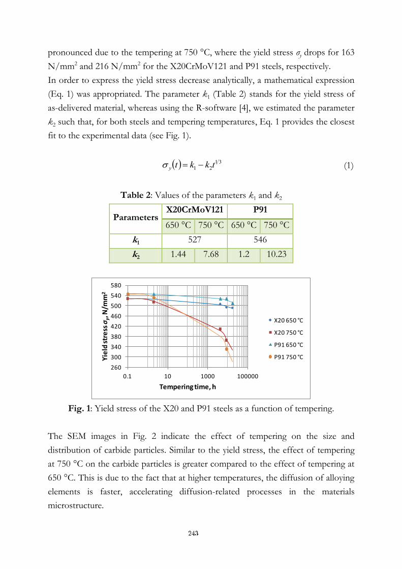
pronounced due to the tempering at 750 °C, where the yield stress σy drops for 163
N/mm2 and 216 N/mm2 for the X20CrMoV121 and P91 steels, respectively.
In order to express the yield stress decrease analytically, a mathematical expression
(Eq. 1) was appropriated. The parameter k1 (Table 2) stands for the yield stress of
as-delivered material, whereas using the R-software [4], we estimated the parameter
k2 such that, for both steels and tempering temperatures, Eq. 1 provides the closest
fit to the experimental data (see Fig. 1).
31
21 tkkty (1)
Table 2: Values of the parameters k1 and k2
Parameters X20CrMoV121 P91
650 °C 750 °C 650 °C 750 °C
k1 527 546
k2 1.44 7.68 1.2 10.23
260
300
340
380
420
460
500
540
580
0.1 10 1000 100000
Yie
ld s
tre
ss σy, N
/mm
2
Tempering time, h
X20 650 °C
X20 750 °C
P91 650 °C
P91 750 °C
Fig. 1: Yield stress of the X20 and P91 steels as a function of tempering.
The SEM images in Fig. 2 indicate the effect of tempering on the size and
distribution of carbide particles. Similar to the yield stress, the effect of tempering
at 750 °C on the carbide particles is greater compared to the effect of tempering at
650 °C. This is due to the fact that at higher temperatures, the diffusion of alloying
elements is faster, accelerating diffusion-related processes in the materials
microstructure.
243
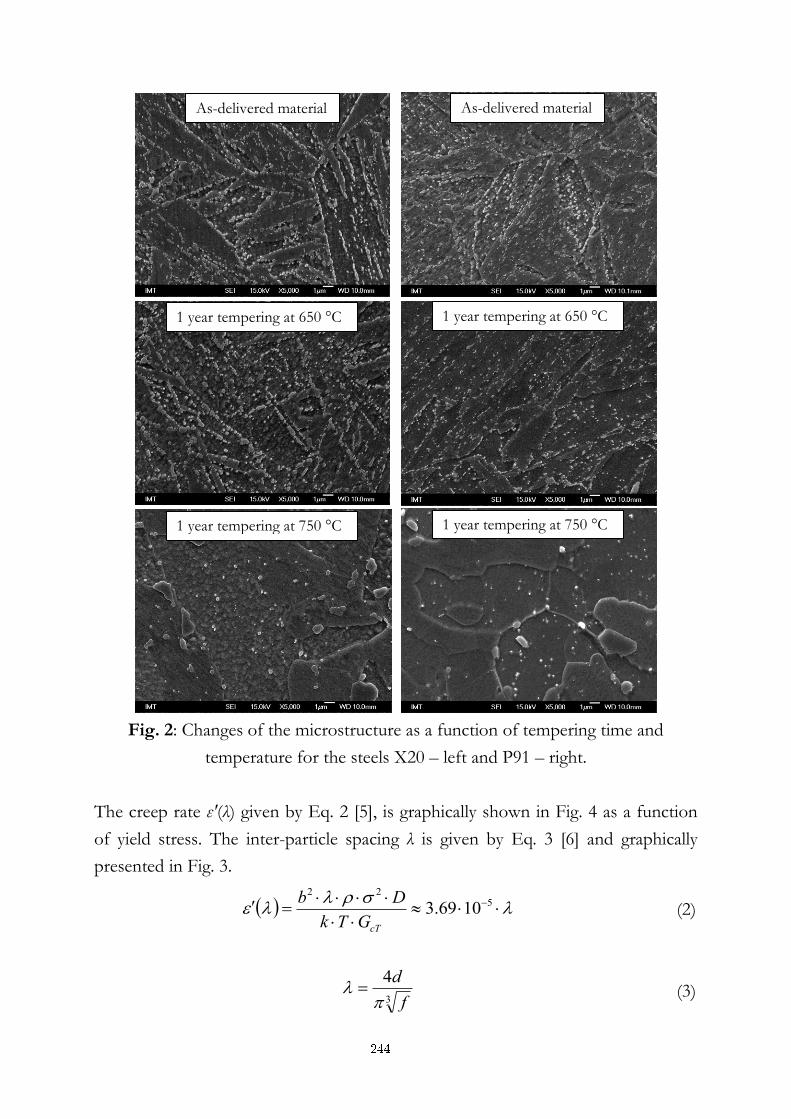
Fig. 2: Changes of the microstructure as a function of tempering time and
temperature for the steels X20 – left and P91 – right.
The creep rate ε'(λ) given by Eq. 2 [5], is graphically shown in Fig. 4 as a function
of yield stress. The inter-particle spacing λ is given by Eq. 3 [6] and graphically
presented in Fig. 3.
5
22
1069.3cTGTk
Db (2)
3
4
f
d
(3)
As-delivered material
1 year tempering at 650 °C
As-delivered material
1 year tempering at 650 °C
1 year tempering at 750 °C 1 year tempering at 750 °C
244
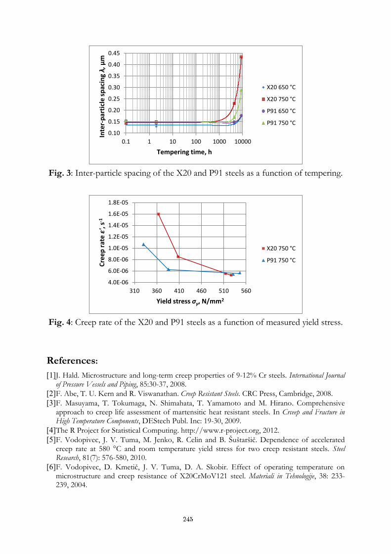
0.10
0.15
0.20
0.25
0.30
0.35
0.40
0.45
0.1 1 10 100 1000 10000
Inte
r-p
arti
cle
spac
ing λ,
μm
Tempering time, h
X20 650 °C
X20 750 °C
P91 650 °C
P91 750 °C
Fig. 3: Inter-particle spacing of the X20 and P91 steels as a function of tempering.
4.0E-06
6.0E-06
8.0E-06
1.0E-05
1.2E-05
1.4E-05
1.6E-05
1.8E-05
310 360 410 460 510 560
Cre
ep r
ate
ε',
s-1
Yield stress σy, N/mm2
X20 750 °C
P91 750 °C
Fig. 4: Creep rate of the X20 and P91 steels as a function of measured yield stress.
References:
[1] J. Hald. Microstructure and long-term creep properties of 9-12% Cr steels. International Journal of Pressure Vessels and Piping, 85:30-37, 2008.
[2] F. Abe, T. U. Kern and R. Viswanathan. Creep Resistant Steels. CRC Press, Cambridge, 2008.
[3] F. Masuyama, T. Tokumaga, N. Shimahata, T. Yamamoto and M. Hirano. Comprehensive approach to creep life assessment of martensitic heat resistant steels. In Crceep and Fracture in High Temperature Components, DEStech Publ. Inc: 19-30, 2009.
[4] The R Project for Statistical Computing. http://www.r-project.org, 2012.
[5] F. Vodopivec, J. V. Tuma, M. Jenko, R. Celin and B. Šuštaršič. Dependence of accelerated creep rate at 580 °C and room temperature yield stress for two creep resistant steels. Steel Research, 81(7): 576-580, 2010.
[6] F. Vodopivec, D. Kmetič, J. V. Tuma, D. A. Skobir. Effect of operating temperature on microstructure and creep resistance of X20CrMoV121 steel. Materiali in Tehnologije, 38: 233-239, 2004.
245
For wider interest
An increased efficiency of the fossil-fired power plants is obtained with higher
operating temperatures and pressures of the steam that enters the turbine. The
standard operating temperatures are 540-565 °C, but during the last 20 years large
efforts have been made to reach the so-called ultra-supercritical (USC) conditions
with the steam parameters up to 300 bars and 620 °C. These conditions require
materials with the high creep-resistance, i.e., the ability to withstand a long-term
loading at high temperatures. This requires a careful material selection and a
periodical checking of its properties and remaining residual lifetime after the
determined period of operation in power plants. The checking of the creep rate and
creep strength is expensive and time-consuming. For this reason, simpler methods
are being developed, which use less expensive and faster tests that enable the
establishment of the state of the built-in steel. One among these methods is to
check the room-temperature mechanical properties and microstructure after
tempering, which simulates the changes in the microstructure and properties that
occur after a longer operation in the power plant (in real conditions) by correlating
the measured properties with the creep rate. The latter is measured using the
standard creep test.
246
Phase transitions of the NaNbO3 submicron-sized powder
between room temperature and 700 °C
Jurij Koruza1,2, Jenny Tellier1,3, Barbara Malič1,2, Marija Kosec1,2
1 Electronic Ceramics Department, Jožef Stefan Institute, Ljubljana, Slovenia
2 Jožef Stefan International Postgraduate School, Ljubljana, Slovenia
3 SPCTS-UMR CNRS 6638, Centre Européen de la Céramique, Limoges, France
[email protected] (email of corresponding author)
Abstract. Phase transition behaviour of the Q polymorph, which was found in
the submicron-sized NaNbO3 powder, was investigated in the temperature
range between room temperature and 700°C. The differential scanning
calorimetry revealed three phase transitions upon heating: Q→R (326.5°C),
T(1)→T(2) (571°C), and T(2)→U (636.8°C). A detailed X-Ray diffraction
measurement combined with the Rietveld analysis was used to determine the
structural changes during the Q→R phase transition. The observed
symmetrisation of the unit cell was related to the increased regularity of the
cuboctahedral cavities and the position of the Na cation.
Keywords: sodium niobate, antiferroelectrics, phase transition, polymorphism.
1 Introduction
Antiferroelectric ceramics have gained increased attention due to their large energy
storage capacity, required for high-performance capacitors [1], and a large volume
change accompanying the field-induced phase transition, which may be used in
high-strain actuator and transducer applications [2]. Sodium niobate (NaNbO3) is a
prototype antiferroelectric. Furthermore, NaNbO3 also exhibits the largest number
of polymorphs* among all oxygen perovskites (Figure 1). The phase transitions in
* The term polymorphism describes the relations among different crystalline modifications
(polymorphs) of the same chemical substance, which typically possess different physical
properties. This phenomenon was observed in many technologically important ceramic materials,
such as ZrO2, Al2O3, SiO2.
247
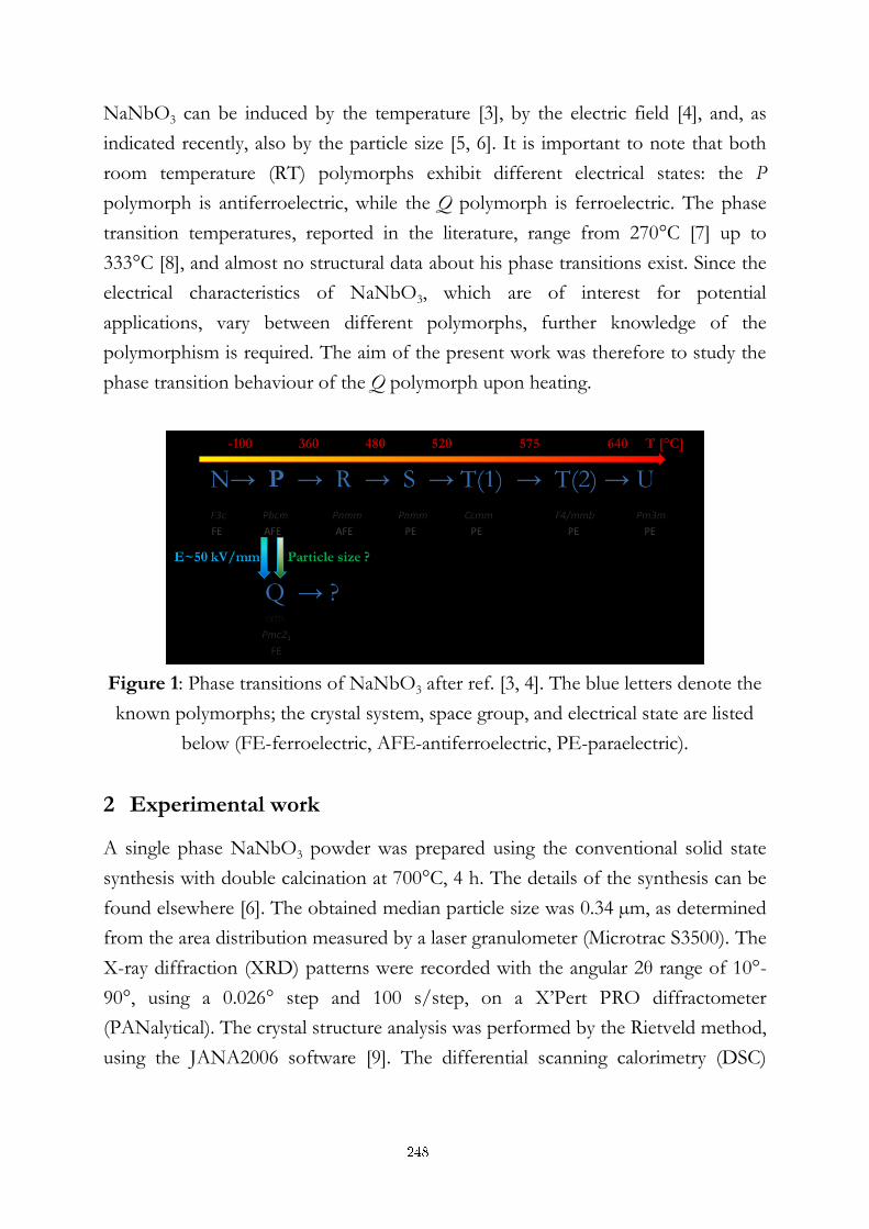
NaNbO3 can be induced by the temperature [3], by the electric field [4], and, as
indicated recently, also by the particle size [5, 6]. It is important to note that both
room temperature (RT) polymorphs exhibit different electrical states: the P
polymorph is antiferroelectric, while the Q polymorph is ferroelectric. The phase
transition temperatures, reported in the literature, range from 270°C [7] up to
333°C [8], and almost no structural data about his phase transitions exist. Since the
electrical characteristics of NaNbO3, which are of interest for potential
applications, vary between different polymorphs, further knowledge of the
polymorphism is required. The aim of the present work was therefore to study the
phase transition behaviour of the Q polymorph upon heating.
Figure 1: Phase transitions of NaNbO3 after ref. [3, 4]. The blue letters denote the
known polymorphs; the crystal system, space group, and electrical state are listed
below (FE-ferroelectric, AFE-antiferroelectric, PE-paraelectric).
2 Experimental work
A single phase NaNbO3 powder was prepared using the conventional solid state
synthesis with double calcination at 700°C, 4 h. The details of the synthesis can be
found elsewhere [6]. The obtained median particle size was 0.34 µm, as determined
from the area distribution measured by a laser granulometer (Microtrac S3500). The
X-ray diffraction (XRD) patterns were recorded with the angular 2θ range of 10°-
90°, using a 0.026° step and 100 s/step, on a X’Pert PRO diffractometer
(PANalytical). The crystal structure analysis was performed by the Rietveld method,
using the JANA2006 software [9]. The differential scanning calorimetry (DSC)
248
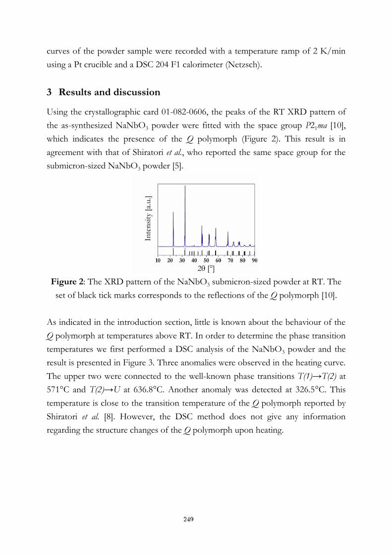
curves of the powder sample were recorded with a temperature ramp of 2 K/min
using a Pt crucible and a DSC 204 F1 calorimeter (Netzsch).
3 Results and discussion
Using the crystallographic card 01-082-0606, the peaks of the RT XRD pattern of
the as-synthesized NaNbO3 powder were fitted with the space group P21ma [10],
which indicates the presence of the Q polymorph (Figure 2). This result is in
agreement with that of Shiratori et al., who reported the same space group for the
submicron-sized NaNbO3 powder [5].
Figure 2: The XRD pattern of the NaNbO3 submicron-sized powder at RT. The
set of black tick marks corresponds to the reflections of the Q polymorph [10].
As indicated in the introduction section, little is known about the behaviour of the
Q polymorph at temperatures above RT. In order to determine the phase transition
temperatures we first performed a DSC analysis of the NaNbO3 powder and the
result is presented in Figure 3. Three anomalies were observed in the heating curve.
The upper two were connected to the well-known phase transitions T(1)→T(2) at
571°C and T(2)→U at 636.8°C. Another anomaly was detected at 326.5°C. This
temperature is close to the transition temperature of the Q polymorph reported by
Shiratori et al. [8]. However, the DSC method does not give any information
regarding the structure changes of the Q polymorph upon heating.
249
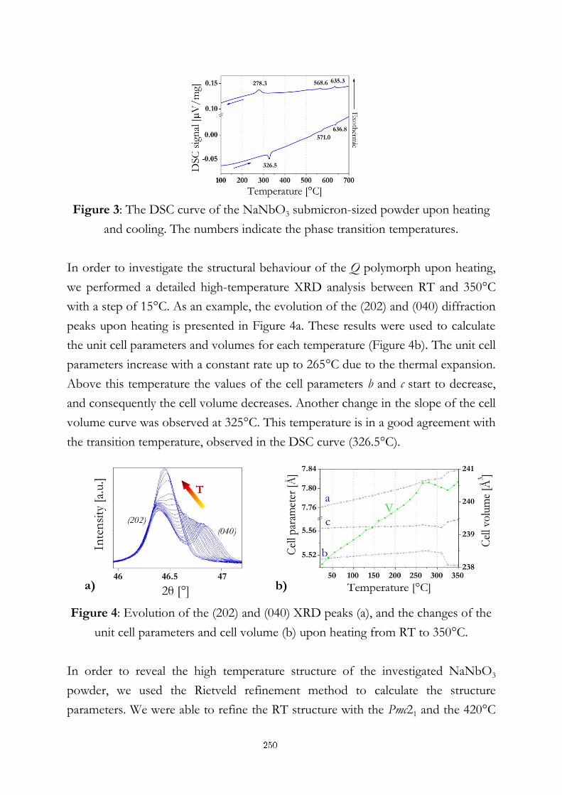
Figure 3: The DSC curve of the NaNbO3 submicron-sized powder upon heating
and cooling. The numbers indicate the phase transition temperatures.
In order to investigate the structural behaviour of the Q polymorph upon heating,
we performed a detailed high-temperature XRD analysis between RT and 350°C
with a step of 15°C. As an example, the evolution of the (202) and (040) diffraction
peaks upon heating is presented in Figure 4a. These results were used to calculate
the unit cell parameters and volumes for each temperature (Figure 4b). The unit cell
parameters increase with a constant rate up to 265°C due to the thermal expansion.
Above this temperature the values of the cell parameters b and c start to decrease,
and consequently the cell volume decreases. Another change in the slope of the cell
volume curve was observed at 325°C. This temperature is in a good agreement with
the transition temperature, observed in the DSC curve (326.5°C).
Figure 4: Evolution of the (202) and (040) XRD peaks (a), and the changes of the
unit cell parameters and cell volume (b) upon heating from RT to 350°C.
In order to reveal the high temperature structure of the investigated NaNbO3
powder, we used the Rietveld refinement method to calculate the structure
parameters. We were able to refine the RT structure with the Pmc21 and the 420°C
250
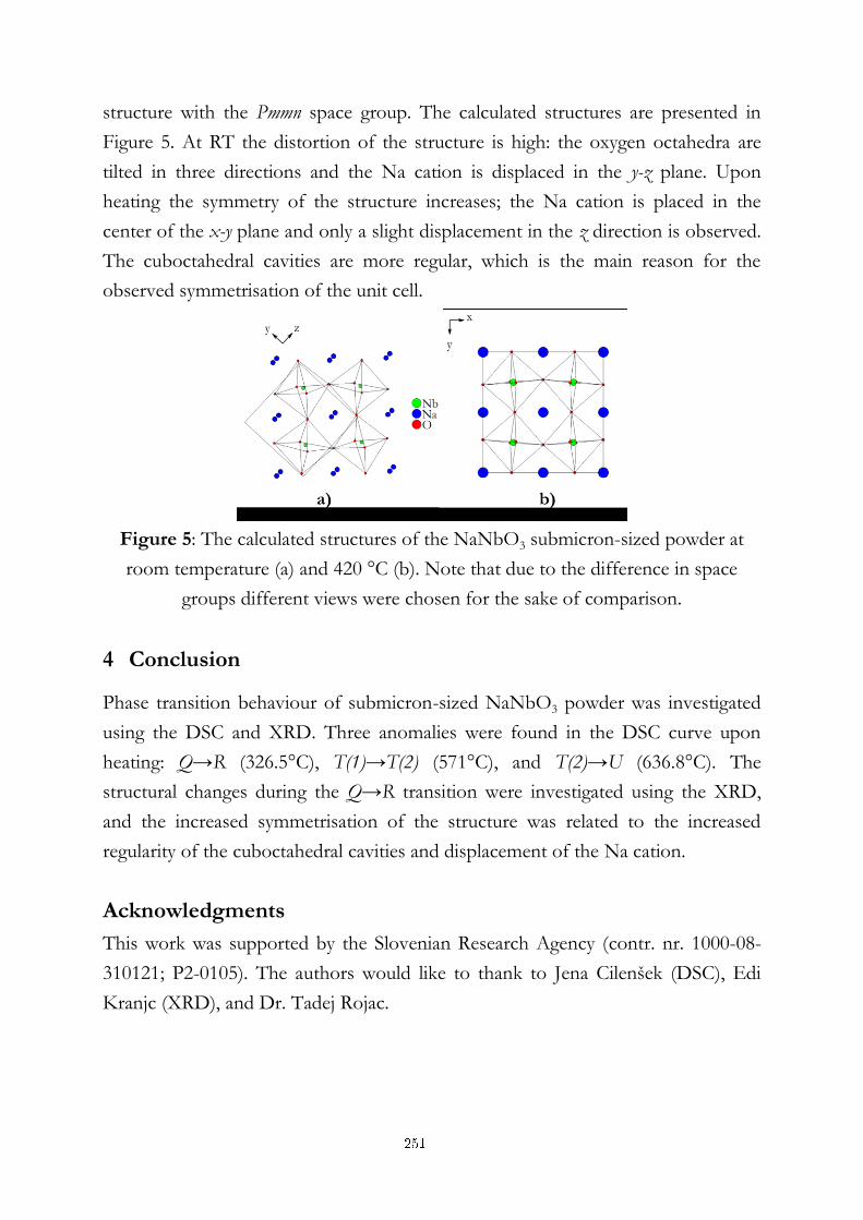
structure with the Pmmn space group. The calculated structures are presented in
Figure 5. At RT the distortion of the structure is high: the oxygen octahedra are
tilted in three directions and the Na cation is displaced in the y-z plane. Upon
heating the symmetry of the structure increases; the Na cation is placed in the
center of the x-y plane and only a slight displacement in the z direction is observed.
The cuboctahedral cavities are more regular, which is the main reason for the
observed symmetrisation of the unit cell.
Figure 5: The calculated structures of the NaNbO3 submicron-sized powder at
room temperature (a) and 420 °C (b). Note that due to the difference in space
groups different views were chosen for the sake of comparison.
4 Conclusion
Phase transition behaviour of submicron-sized NaNbO3 powder was investigated
using the DSC and XRD. Three anomalies were found in the DSC curve upon
heating: Q→R (326.5°C), T(1)→T(2) (571°C), and T(2)→U (636.8°C). The
structural changes during the Q→R transition were investigated using the XRD,
and the increased symmetrisation of the structure was related to the increased
regularity of the cuboctahedral cavities and displacement of the Na cation.
Acknowledgments
This work was supported by the Slovenian Research Agency (contr. nr. 1000-08-
310121; P2-0105). The authors would like to thank to Jena Cilenšek (DSC), Edi
Kranjc (XRD), and Dr. Tadej Rojac.
251
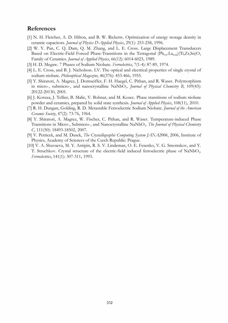
References
[1] N. H. Fletcher, A. D. Hilton, and B. W. Ricketts. Optimization of energy storage density in
ceramic capacitors. Journal of Physics D-Applied Physics, 29(1): 253-258, 1996.
[2] W. Y. Pan, C. Q. Dam, Q. M. Zhang, and L. E. Cross. Large Displacement Transducers Based on Electric-Field Forced Phase-Transitions in the Tetragonal (Pb0.97La0.02)(Ti,Zr,Sn)O3
Family of Ceramics. Journal of Applied Physics, 66(12): 6014-6023, 1989.
[3] H. D. Megaw. 7 Phases of Sodium Niobate. Ferroelectrics, 7(1-4): 87-89, 1974.
[4] L. E. Cross, and B. J. Nicholson. LV. The optical and electrical properties of single crystal of
sodium niobate. Philosophical Magazine, 46(376): 453-466, 1955.
[5] Y. Shiratori, A. Magrez, J. Dornseiffer, F. H. Haegel, C. Pithan, and R. Waser. Polymorphism in micro-, submicro-, and nanocrystalline NaNbO3. Journal of Physical Chemistry B, 109(43):
20122-20130, 2005.
[6] J. Koruza, J. Tellier, B. Malic, V. Bobnar, and M. Kosec. Phase transitions of sodium niobate
powder and ceramics, prepared by solid state synthesis. Journal of Applied Physics, 108(11), 2010. [7] R. H. Dungan, Golding, R. D. Metastable Ferroelectric Sodium Niobate. Journal of the American
Ceramic Society, 47(2): 73-76, 1964.
[8] Y. Shiratori, A. Magrez, W. Fischer, C. Pithan, and R. Waser. Temperature-induced Phase Transitions in Micro-, Submicro-, and Nanocrystalline NaNbO3. The Journal of Physical Chemistry
C, 111(50): 18493-18502, 2007. [9] V. Petricek, and M. Dusek, The Crystallographic Computing System JANA2006, 2006, Institute of
Physics, Academy of Scienecs of the Czech Republic: Prague. [10] V. A. Shuvaeva, M. Y. Antipin, R. S. V. Lindeman, O. E. Fesenko, V. G. Smotrakov, and Y.
T. Struchkov. Crystal structure of the electric-field induced ferroelectric phase of NaNbO3.
Ferroelectrics, 141(1): 307-311, 1993.
252

For wider interest
The functional properties of ceramic materials directly depend on their crystal
structure, which changes upon changing the temperature. Therefore the
understanding of the crystal structure and the phase transitions is of great
importance when the materials are to be used in devices for various applications.
In the present work we demonstrate the implementation of the two complementary
analytical techniques for investigation of phase transitions and crystal structure of
materials: the differential scanning calorimetry (DSC) and the X-Ray diffraction
(XRD) combined with the Rietveld analysis. The first one was used to determine
the transition temperatures, while the second one enabled the insight into the
crystal structure of the material.
253
Environmental Friendly Potassium Sodium Niobate Based Thin Films from Solutions
Alja Kupec1,2,3 Barbara Malič1,3,4,5 and Marija Kosec1,2,3
1 Electronic Ceramics Department, Jožef Stefan Institute, Ljubljana, Slovenia
2 Centre of Excellence NAMASTE, Ljubljana, Slovenia
3Jožef Stefan International Postgraduate School, Ljubljana, Slovenia
4Centre of Excellence on Nanoscience and Nanotechnology, Ljubljana, Slovenia.
5Centre of Excellence SPACE-SI, Ljubljana, Slovenia.
Abstract. We present the synthesis of ~250 nm thick K0.5Na0.5NbO3 thin
films on platinized silicon substrates from alkoxide-based solutions with the
stoichiometric composition and with the 5 or 10 mole % potassium acetate
excess. The films crystallized into a pure perovskite phase, but depending on
the amount of the alkali excess in solutions, they consisted of ~50 nm or of
~200 nm large grains. The fine-grained film from the solution with the 5 mole
% alkali excess had the dielectric permittivity and losses of 610 and 1.5 %,
respectively, and exhibited a ferroelectric polarisation–electric field
dependence at room temperature.
Keywords: Chemical Solution Deposition, Thin film, Lead-free, Ferroelectric
1 Introduction
In the field of piezoelectric materials, lead-based complex perovskite systems are
widely used due to their good functional response. The main drawback of these
materials is the toxicity of lead compounds and, as a consequence, the research of
environmentally friendly ceramic materials has been intensified in the last years.
Potassium sodium niobate (KxNa1-x)NbO3 has been considered as one of the
candidates that could replace lead based perovskites. It is a solid solution of
ferroelectric KNbO3 and antiferroelectric NaNbO3 with the best dielectric and
piezoelectric properties near x = 0.5 (KNN).[1] The major problems related to this
material are the humidity, sensitivity and volatilization of alkali compounds, which
254
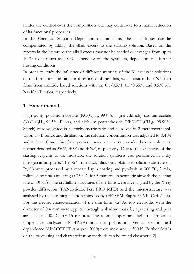
hinder the control over the composition and may contribute to a major reduction
of its functional properties.
In the Chemical Solution Deposition of thin films, the alkali losses can be
compensated by adding the alkali excess to the starting solution. Based on the
reports in the literature, the alkali excess may not be needed or it ranges from up to
10 % to as much as 20 %, depending on the synthesis, deposition and further
heating conditions.
In order to study the influence of different amounts of the K- excess in solutions
on the formation and functional response of the films, we deposited the KNN thin
films from alkoxide based solutions with the 0.5/0.5/1, 0.5/0.55/1 and 0.5/0.6/1
Na/K/Nb ratios, respectively.
1 Experimental
High purity potassium acetate (KO2C2H3, 99+%, Sigma Aldrich), sodium acetate
(NaO2C2H3, 99.5%, Fluka), and niobium pentaethoxide (Nb(OCH2CH3)5, 99.99%,
Starck) were weighted in a stoichiometric ratio and dissolved in 2-methoxyethanol.
Upon a 4 h reflux and distillation, the solution concentration was adjusted to 0.4 M
and 0, 5 or 10 mole % of the potassium-acetate excess was added to the solutions,
further denoted as Stoich, +5K and +10K, respectively. Due to the sensitivity of the
starting reagents to the moisture, the solution synthesis was performed in a dry
nitrogen atmosphere. The ~240 nm thick films on a platinized silicon substrate (or
Pt/Si) were processed by a repeated spin coating and pyrolysis at 300 °C, 2 min,
followed by final annealing at 750 °C for 5 minutes, in synthetic air with the heating
rate of 10 K/s. The crystalline structures of the films were investigated by the X-ray
powder diffraction (PANalyticalX`Pert PRO MPD) and the microstructure was
analysed by the scanning electron microscopy (FE-SEM: Supra 35 VP, Carl Zeiss).
For the electric characterization of the thin films, Cr/Au top electrodes with the
diameter of 0.4 mm were applied through a shadow mask by sputtering and post
annealed at 400 °C, for 15 minutes. The room temperature dielectric properties
(impedance analyzer HP 4192A) and the polarisation versus electric field
dependence (AixACCT TF Analyzer 2000) were measured at 300 K. Further details
on the processing and characterization methods can be found elsewhere.[2]
255
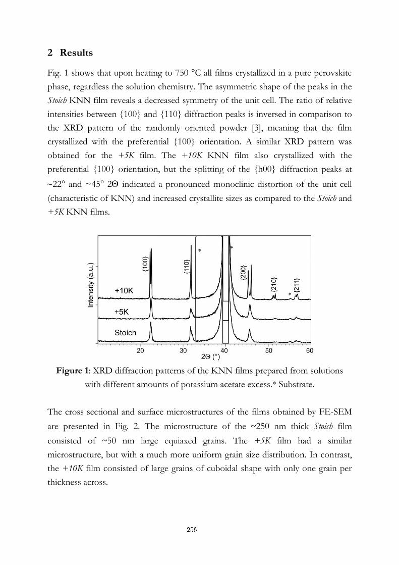
2 Results
Fig. 1 shows that upon heating to 750 °C all films crystallized in a pure perovskite
phase, regardless the solution chemistry. The asymmetric shape of the peaks in the
Stoich KNN film reveals a decreased symmetry of the unit cell. The ratio of relative
intensities between {100} and {110} diffraction peaks is inversed in comparison to
the XRD pattern of the randomly oriented powder [3], meaning that the film
crystallized with the preferential {100} orientation. A similar XRD pattern was
obtained for the +5K film. The +10K KNN film also crystallized with the
preferential {100} orientation, but the splitting of the {h00} diffraction peaks at
22° and ~45° 2 indicated a pronounced monoclinic distortion of the unit cell
(characteristic of KNN) and increased crystallite sizes as compared to the Stoich and
+5K KNN films.
Figure 1: XRD diffraction patterns of the KNN films prepared from solutions
with different amounts of potassium acetate excess.* Substrate.
The cross sectional and surface microstructures of the films obtained by FE-SEM
are presented in Fig. 2. The microstructure of the ~250 nm thick Stoich film
consisted of ~50 nm large equiaxed grains. The +5K film had a similar
microstructure, but with a much more uniform grain size distribution. In contrast,
the +10K film consisted of large grains of cuboidal shape with only one grain per
thickness across.
256
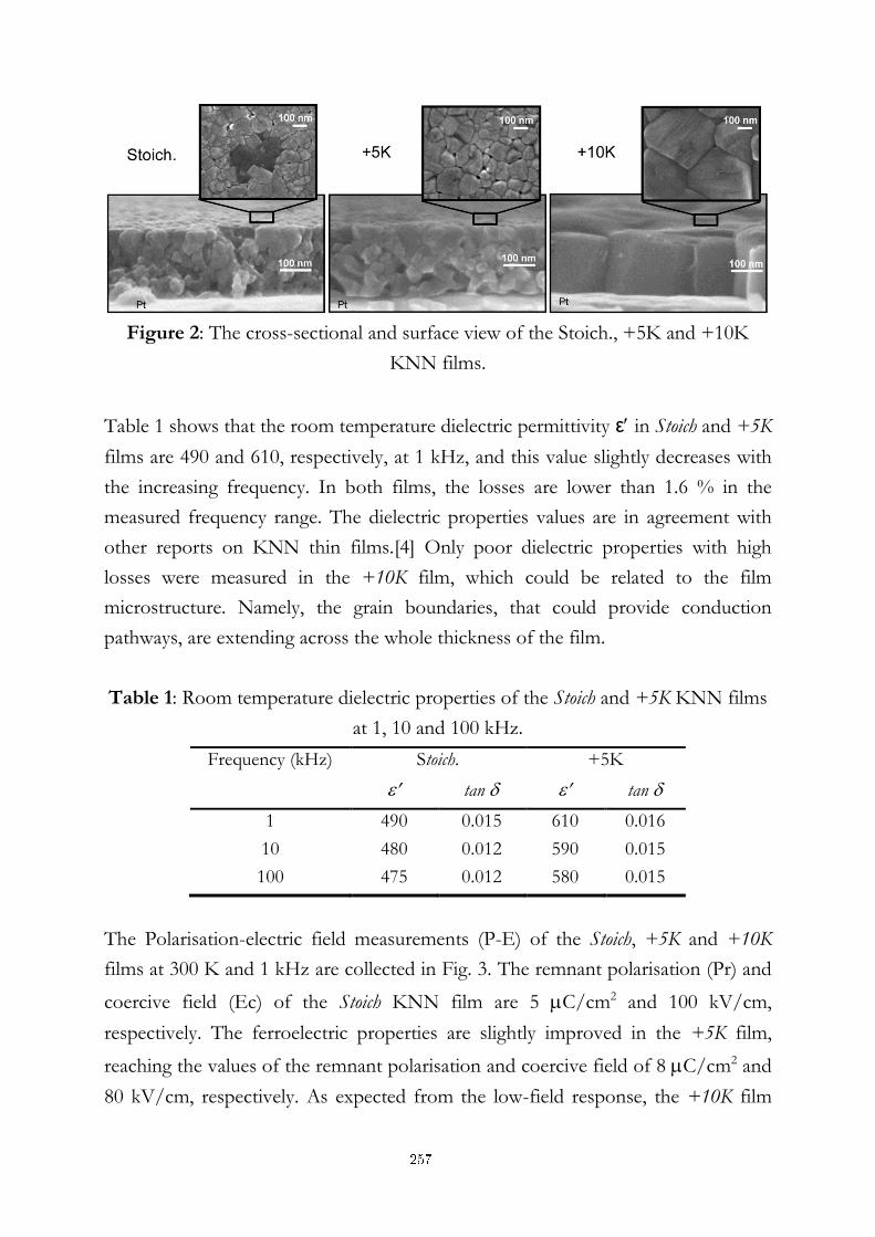
Figure 2: The cross-sectional and surface view of the Stoich., +5K and +10K
KNN films.
Table 1 shows that the room temperature dielectric permittivity ε in Stoich and +5K
films are 490 and 610, respectively, at 1 kHz, and this value slightly decreases with
the increasing frequency. In both films, the losses are lower than 1.6 % in the
measured frequency range. The dielectric properties values are in agreement with
other reports on KNN thin films.[4] Only poor dielectric properties with high
losses were measured in the +10K film, which could be related to the film
microstructure. Namely, the grain boundaries, that could provide conduction
pathways, are extending across the whole thickness of the film.
Table 1: Room temperature dielectric properties of the Stoich and +5K KNN films
at 1, 10 and 100 kHz.
Frequency (kHz) Stoich. +5K
tan tan
1 490 0.015 610 0.016
10 480 0.012 590 0.015
100 475 0.012 580 0.015
The Polarisation-electric field measurements (P-E) of the Stoich, +5K and +10K
films at 300 K and 1 kHz are collected in Fig. 3. The remnant polarisation (Pr) and
coercive field (Ec) of the Stoich KNN film are 5 C/cm2 and 100 kV/cm,
respectively. The ferroelectric properties are slightly improved in the +5K film,
reaching the values of the remnant polarisation and coercive field of 8 C/cm2 and
80 kV/cm, respectively. As expected from the low-field response, the +10K film
257
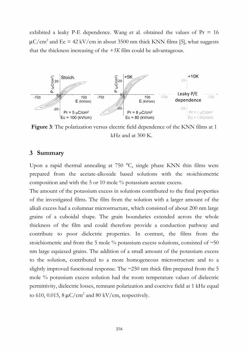
exhibited a leaky P-E dependence. Wang et al. obtained the values of Pr = 16
C/cm2 and Ec = 42 kV/cm in about 3500 nm thick KNN films [5], what suggests
that the thickness increasing of the +5K film could be advantageous.
Figure 3: The polarization versus electric field dependence of the KNN films at 1
kHz and at 300 K.
3 Summary
Upon a rapid thermal annealing at 750 °C, single phase KNN thin films were
prepared from the acetate-alkoxide based solutions with the stoichiometric
composition and with the 5 or 10 mole % potassium acetate excess.
The amount of the potassium excess in solutions contributed to the final properties
of the investigated films. The film from the solution with a larger amount of the
alkali excess had a columnar microstructure, which consisted of about 200 nm large
grains of a cuboidal shape. The grain boundaries extended across the whole
thickness of the film and could therefore provide a conduction pathway and
contribute to poor dielectric properties. In contrast, the films from the
stoichiometric and from the 5 mole % potassium excess solutions, consisted of ~50
nm large equiaxed grains. The addition of a small amount of the potassium excess
to the solution, contributed to a more homogeneous microstructure and to a
slightly improved functional response. The ~250 nm thick film prepared from the 5
mole % potassium excess solution had the room temperature values of dielectric
permittivity, dielectric losses, remnant polarization and coercive field at 1 kHz equal
to 610, 0.015, 8 C/cm2 and 80 kV/cm, respectively.
258

References:
[1] Y. Saito; H. Takao; T. Tani, et al. Lead-free Piezoceramics. Nature, 432: 84-87, 2004. [2] A. Kupec; B. Malič; J. Tellier, et al. Lead-free Ferroelectric Potassium Sodium Niobate Thin Films from Solution: Composition and Structure. Journal of the American Ceramic Society, 95: 515-523, 2012. [3] J. Tellier; B. Malič; B. Dkhil, et al. Crystal Structure and Phase Transitions of Sodium Potassium Niobate Perovskites. Solid State Sciences, 11: 320-324, 2009. [4] K. Tanaka; H. Hayashi; K. I. Kakimoto, et al. Effect of (Na,K)-excess Precursor Solutions on Alkoxy-derived (Na,K)NbO3 Powders and Thin Films. Japanese Journal of Applied Physics, 46: 6964-6970, 2007. [5] L. Wang; K. Yao; P. C. Goh, et al. Volatilization of Alkali Ions and Effects of Molecular Weight of Polyvinylpyrrolidone Introduced in Solution-derived Ferroelectric K0.5Na0.5NbO3 Films. Journal of Materials Research, 24: 3516-3522, 2009.
259
For wider interest
Piezoelectric ceramic materials are used as sensors, actuators and micro-electro
mechanical devices (MEMS). The continuous trend in miniaturization of
micromechanic and microelectronic components has provided applications for thin
films: the nanomaterials with thicknesses of less than 1 m.
The properties of thin film-structures often differ from those of bulk ceramics and
need to be understood in order to produce new devices. Thin films can be prepared
by dry (physical) and wet (chemical) techniques. The former enable the preparation
of high quality thin films but with an expensive equipment, while the latter are
relatively quick, inexpensive and offer a good variety of possibilities for an easy
modification of the composition for improvements in structure properties of
functional thin films.
The basic steps of Chemical Solution Deposition (CSD) of thin films include the
synthesis of the precursor solution, the deposition of the solution on the substrate,
and the heat treatment of the deposited film. Among CSD, the alkoxide based sol-
gel route enables the synthesis of different heterometallic solutions and gives the
possibility to tailor the reactivity of the starting compounds. The detailed
investigations of impacts of precursor solutions, nucleation and growth of the
microstructure have led to increase the variety of materials systems that can be
prepared and to tremendous improvements in the quality of the films.
The lead zirconate titanate based solid solutions (Pb(Zr,Ti)O3, PZT) are among the
most widely studied materials for piezoelectric thin films. However, in the past
years the research of lead-free ceramic materials intensified as a consequence of the
increased awareness of the society towards the protection of the environment and
human health from a hazardous substance, lead.
260
The Effect of the Firing Temperature on the Properties of LTCC
Kostja Makarovič1,3,*, Anton Meden2,3, Marko Hrovat1,3, Janez Holc1,3,
Andreja Benčan1,3, Aleš Dakskobler1,3, Darko Belavič1,3,4, Marija Kosec1,3
1 Jožef Stefan Institute, Jamova 39, SI-1000 Ljubljana, Slovenia
2 University of Ljubljana, Faculty of Chemistry and Chemical Technology, Aškerčeva
cesta 5, SI-1000 Ljubljana, Slovenia
3 CoE NAMASTE, Jamova 39, SI-1000 Ljubljana, Slovenia
4 HIPOT-RR, Šentpeter 18, 8222 Otočec, Slovenia
Abstract. The influence of the firing temperature on the phase composition,
microstructure and biaxial flexural strength of the DuPont 951 low temperature
cofired ceramics (LTCC) material is presented. During the firing at temperatures
around 700 °C, Al2O3 starts to partially dissolve in a low viscosity glass phase and
the dissolution continues up to 800 °C. The anorthite phase starts to crystallize at
875 °C from the glass phase on the surface of the Al2O3 particles. The mass
fraction of the anorthite increases with increasing temperature until it reaches a
plateau value of around 22 w.% at 950 °C or higher temperatures. The biaxial
flexural strength of the LTCC increases with increasing firing temperature from
135 MPa (at 800 °C) to around 214 MPa (at 850 °C). In this temperature range
the major effect on the biaxial flexural strength of the LTCC is that of porosity.
Further, increase of the biaxial flexural strength of the LTCC up to around 300
MPa is correlated with the crystallization of the anorthite.
Keywords: LTCC, firing temperatures, phase composition, biaxial flexural
strength, anorthite.
1 Introduction
The low temperature cofired ceramics (LTCCs) technology is used for substrates in
multilayer ceramic circuits, mainly for telecommunications, automotive, and medical
applications. In recent times LTCCs were also recognized as useful materials for
producing complex 3D structures with buried cavities and channels or so-called
micro-electro-mechanical systems (MEMS).[1]
261
The majority of LTCCs are glass-ceramics composites. These glass-ceramic
composites are usually designed to yield partial glass crystallization during the firing,
which then minimizes the amount of glass the phase in the composite and influences
the mechanical and electrical properties of the glass-ceramic material. Driven by the
needs of the target application, the interactions of different glasses with ceramic fillers
during firing as well as the phases, which crystallize from the glasses, were extensively
studied.[1-3]
The main physical properties of commercially available LTCCs processed, using the
parameters, which are specified by the producer, are available in datasheets and other
open literature. However, the production of large or complex 3D LTCC structures
requires a different, rather longer, firing procedure [4]. Unconventional firing
processes affect the final functional properties of the LTCC material. To the best of
our knowledge there is not much data available in the open literature about the
influence of different firing conditions, such as a firing temperature, on the
microstructure, phase composition, and, consequently, on the functional properties of
the LTCC.
2 Experimental
For the investigation the mostly used commercial LTCC DuPont® Green Tape™
951[5] was chosen. The green thickness of the used tape was 254 µm. Thicker samples
were prepared by laminating the tapes at a pressure of 20 MPa at 80 °C for 15
minutes and cutting with a blade cutter.
The samples were heated at a heating rate of 7 K/minute to 450 °C and held there for
60 minutes at 450 °C to burn out the organic binder. Further, heating to the
maximum temperature and cooling to room temperature was performed at a rate of
10 K/minute. The maximum temperatures were 600 °C, 700 °C, 750 °C, 800 °C, 850
°C, 875 °C, 900 °C, 950 °C and 1000 °C with a dwell time of 15 minutes.
To determine the phase composition, the fired samples were ground and analysed
with a PANalytical X'Pert PRO MPD X-ray diffractometer (Almelo, Netherland). The
XRD diffractometer was operated with a Cu Kα1 configuration using a wavelength of
1.54060 Å in the angle 2θ range between 10 ° and 70 °, a step of 0.034 ° and an
integration time of 100 s. The ground samples were analyzed in a Φ = 27 mm holder
with a powder depth of 2.5 mm. The analyses of the diffraction patterns and the
262
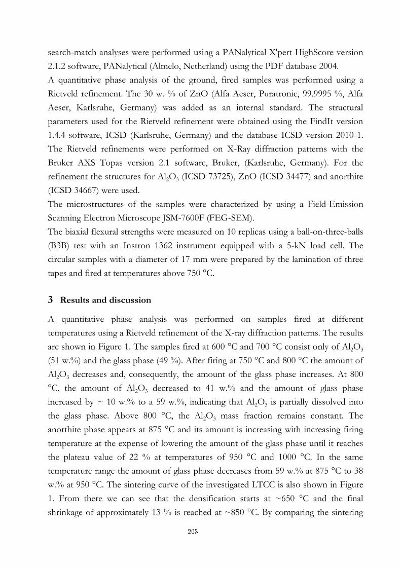
search-match analyses were performed using a PANalytical X'pert HighScore version
2.1.2 software, PANalytical (Almelo, Netherland) using the PDF database 2004.
A quantitative phase analysis of the ground, fired samples was performed using a
Rietveld refinement. The 30 w. % of ZnO (Alfa Aeser, Puratronic, 99.9995 %, Alfa
Aeser, Karlsruhe, Germany) was added as an internal standard. The structural
parameters used for the Rietveld refinement were obtained using the FindIt version
1.4.4 software, ICSD (Karlsruhe, Germany) and the database ICSD version 2010-1.
The Rietveld refinements were performed on X-Ray diffraction patterns with the
Bruker AXS Topas version 2.1 software, Bruker, (Karlsruhe, Germany). For the
refinement the structures for Al2O3 (ICSD 73725), ZnO (ICSD 34477) and anorthite
(ICSD 34667) were used.
The microstructures of the samples were characterized by using a Field-Emission
Scanning Electron Microscope JSM-7600F (FEG-SEM).
The biaxial flexural strengths were measured on 10 replicas using a ball-on-three-balls
(B3B) test with an Instron 1362 instrument equipped with a 5-kN load cell. The
circular samples with a diameter of 17 mm were prepared by the lamination of three
tapes and fired at temperatures above 750 °C.
3 Results and discussion
A quantitative phase analysis was performed on samples fired at different
temperatures using a Rietveld refinement of the X-ray diffraction patterns. The results
are shown in Figure 1. The samples fired at 600 °C and 700 °C consist only of Al2O3
(51 w.%) and the glass phase (49 %). After firing at 750 °C and 800 °C the amount of
Al2O3 decreases and, consequently, the amount of the glass phase increases. At 800
°C, the amount of Al2O3 decreased to 41 w.% and the amount of glass phase
increased by ~ 10 w.% to a 59 w.%, indicating that Al2O3 is partially dissolved into
the glass phase. Above 800 °C, the Al2O3 mass fraction remains constant. The
anorthite phase appears at 875 °C and its amount is increasing with increasing firing
temperature at the expense of lowering the amount of the glass phase until it reaches
the plateau value of 22 % at temperatures of 950 °C and 1000 °C. In the same
temperature range the amount of glass phase decreases from 59 w.% at 875 °C to 38
w.% at 950 °C. The sintering curve of the investigated LTCC is also shown in Figure
1. From there we can see that the densification starts at ~650 °C and the final
shrinkage of approximately 13 % is reached at ~850 °C. By comparing the sintering
263
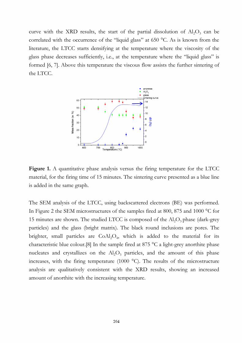
curve with the XRD results, the start of the partial dissolution of Al2O3 can be
correlated with the occurrence of the “liquid glass” at 650 °C. As is known from the
literature, the LTCC starts densifying at the temperature where the viscosity of the
glass phase decreases sufficiently, i.e., at the temperature where the “liquid glass” is
formed [6, 7]. Above this temperature the viscous flow assists the further sintering of
the LTCC.
Figure 1. A quantitative phase analysis versus the firing temperature for the LTCC
material, for the firing time of 15 minutes. The sintering curve presented as a blue line
is added in the same graph.
The SEM analysis of the LTCC, using backscattered electrons (BE) was performed.
In Figure 2 the SEM microstructures of the samples fired at 800, 875 and 1000 °C for
15 minutes are shown. The studied LTCC is composed of the Al2O3 phase (dark-grey
particles) and the glass (bright matrix). The black round inclusions are pores. The
brighter, small particles are CoAl2O4, which is added to the material for its
characteristic blue colour.[8] In the sample fired at 875 °C a light-grey anorthite phase
nucleates and crystallizes on the Al2O3 particles, and the amount of this phase
increases, with the firing temperature (1000 °C). The results of the microstructure
analysis are qualitatively consistent with the XRD results, showing an increased
amount of anorthite with the increasing temperature.
264
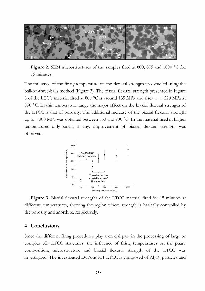
Figure 2. SEM microstructures of the samples fired at 800, 875 and 1000 °C for
15 minutes.
The influence of the firing temperature on the flexural strength was studied using the
ball-on-three-balls method (Figure 3). The biaxial flexural strength presented in Figure
3 of the LTCC material fired at 800 °C is around 135 MPa and rises to ~ 220 MPa at
850 °C. In this temperature range the major effect on the biaxial flexural strength of
the LTCC is that of porosity. The additional increase of the biaxial flexural strength
up to ~300 MPa was obtained between 850 and 900 °C. In the material fired at higher
temperatures only small, if any, improvement of biaxial flexural strength was
observed.
Figure 3. Biaxial flexural strengths of the LTCC material fired for 15 minutes at
different temperatures, showing the region where strength is basically controlled by
the porosity and anorthite, respectively.
4 Conclusions
Since the different firing procedures play a crucial part in the processing of large or
complex 3D LTCC structures, the influence of firing temperatures on the phase
composition, microstructure and biaxial flexural strength of the LTCC was
investigated. The investigated DuPont 951 LTCC is composed of Al2O3 particles and
1 m 1 m 1 m
800 °C 875 °C 1000 °C
Al2O3
glass
anorthite
CoAl2O4
Al2O3
pore
glass anorthite
265
glass. At 675 °C the LTCC starts to densify after the “liquid glass” is formed. Close to
this temperature the particles of Al2O3 start to dissolve and the amount of glassy
phase increases up to 800 °C. From 675 °C to ~875 °C the sintering of the LTCC
takes place and the material is fully sintered at 875 °C. The anorthite crystallizes on
the surface of the Al2O3 particles. The amount increases with the increasing firing
temperature or time, until it reaches the plateau value at around 22 w.%. The amount
of the glass is reduced accordingly. The biaxial flexural strength of the LTCC material
fired at 800 °C is around 135 MPa and rises to ~ 220 MPa at 850 °C. The additional
improvement of the biaxial flexural strength up to ~300 MPa was obtained between
850 and 900 °C when the anorthite crystallizes around the alumina particles. In the
material fired at higher temperatures only small, if any, improvement of biaxial
flexural strength can be observed.
Acknowledgments
The Slovenian Research Agency is acknowledged for its financial support of the
projects “Ceramic materials for 3D structures and study of functional properties” (L2-
2343), the Young Researcher project 100-009-310145. The financial support of the
CoE NAMASTE is gratefully acknowledged.
References
[1] Imanaka, Y., Multilayered low temperature cofired ceramics (LTCC) technology, Springer: 2005. [2] Müller, R., Meszaros, R., Peplinski, B., Reinsch, S., Eberstein, M., Schiller, W. A., Deubener, J., "Dissolution of Alumina, Sintering, and Crystallization in Glass Ceramic Composites for LTCC", Journal of the American Ceramic Society, 92 (8): 1703-1708, 2009. [3] Imanaka, Y., Yamazaki, K., Aoki, S., Kamehara, N., Niwa, K., "Effects of alumina addition on crystallization of borosilicate glass", Journal of the Ceramic Society of Japan, 97 (3): 309-313, 1989. [4] Khoong, L. E., Tan, Y. M., Lam, Y. C., "Overview on fabrication of three-dimensional structures in multi-layer ceramic substrate", Journal of the European Ceramic Society, 30 (10): 1973-1987, 2010 [5] DuPont® "951 Green Tape™" Datasheet, In DuPont Microcircuit Materials, 1-2, 2001. [6] Kemethmüller, S., Hagymasi, M., Stiegelschmitt, A., Roosen, A., "Viscous Flow as the Driving Force for the Densification of Low-Temperature Co-Fired Ceramics", Journal of the American Ceramic Society, 90 (1): 64-70, 2007. [7] Cole, S., Wellfair, G., High temperature viscosity control in multi-layer glasses - a new concept, Proceedings of the ISHM Symposium, Boston, Massachusetts: 25-34, 1974. [8] Jones, W. K., Liu, Y., Larsen, B., Wang, P., Zampino, M., Chemical, Structural, and Mechanical Properties of the LTCC Tapes, Proceedings of the IMAPS International Symposium on Microelectronics, Boston, Massachusetts: 469-473, 2000.
266
For wider interest
The low-temperature co-fired ceramic (LTCC) is an important composite glass-
ceramic material in the production of ceramic multilayer structures mainly for the
telecommunications, automotive, and medical applications. In recent times the
LTCCs were also recognized as useful materials for producing complex 3D structures
with buried cavities and channels or so-called micro-electro-mechanical systems
(MEMS). For MEMS structures are very important their chemical, thermal and
mechanical properties, while in electronic circuits of the main importance are
electrical properties.
The characteristics of the commercially available LTCC tapes processed under
prescribed procedures are available in the datasheets and other open literature;
however, the large and complex multilayer structures are usually fired for longer firing
times and/or, higher firing temperatures, than the relatively thin LTCC tapes. The
firing procedures determine the phase composition and the microstructure, which
both influence the physical properties, such as the mechanical and thermal properties
of the material.
Our research is focused on the study of the effects of the firing temperature and firing
time on the phase composition, microstructure, mechanical properties and coefficient
of thermal expansion of the material in order to understand the processes during the
firing and their effect on the final properties of the material. In order to reach the
desired final properties of devices, the mechanisms of the sintering and the
crystallization of glass material and their influences on the physical properties must be
known. With this knowledge the new material with designed properties can be
developed.
267
Conformational preferences of alanine tripeptide in water, trifluoroethanol and dimethyl sulfoxide studied by vibrational spectroscopy
Andreja Mirtič1, Jože Grdadolnik1,2
1 National Institute of Chemistry, Ljubljana, Slovenia
2 EN-FIST Centre of Excellence, Ljubljana, Slovenia
Abstract. Alanine tripeptide is a good model molecule to analyze a
conformational distribution of an unstructured peptide backbone, to study a
competition between the intra- and intermolecular hydrogen-bonding, as well
as the favourable solvation conditions. In our work, we used three different
spectroscopic techniques, the Raman and infrared (IR) spectroscopy, and the
vibrational circular dichroism (VCD) that are conformation-sensitive and
provide information about hydrogen bonded carbonyl groups (amide I region)
and amino groups (amide II and III regions in the spectrum) of a peptide
backbone. Alanine tripeptide in water exhibits low-frequency bands in the
amide I region at 1618 cm-1 and in the amide III region at 1260 cm-1,
suggesting a strong intramolecular hydrogen bond indicative of a C7
conformation. This bond is disrupted in dimethyl sulfoxide (DMSO) where
the solvent molecules interact with amino groups of alanine tripeptide forming
intermolecular hydrogen bonds. A similar situation is found in trifluoroethanol
(TFE) where alanine tripeptide forms mainly intermolecular hydrogen bonds
with a hydrogen donor from solvent molecules.
Keywords: alanine tripeptide, Raman, infrared spectroscopy, vibrational
circular dichroism, conformation, hydrogen bond, C7 conformation
Introduction
Each amino acid has its intrinsic backbone preferences (,) that determine the
local structure in unfolded peptide chains and may guide the folding process at
268
early stages of the folding. Alanine amino acid is a good model system due to its
simpler vibrational spectra and thus an easier comparison of experimental data with
the theory. A preliminary study of the amide III region in IR and Raman spectra of
dipeptides showed that the population of alanine dipeptide in water is around 60%
of polyproline II (PII), 11% of the right handed helix (R) and 29% of the beta ()
conformation [1]. The two main factors determine the conformational preferences
of dipeptides: the competition between the intra- and intermolecular H-bonding,
and the favourable solvation conditions [2]. In this work, we report the study of a
conformational equilibrium of alanine tripeptide by characterizing the preferred
conformations of the peptide backbone in water, proton donor solvent (TFE) and
proton acceptor solvent (DMSO), respectively.
Materials and Methods
We used alanine tripeptide with N-terminal blocking group acetyl (Ac) and C-
terminal blocking group methylamine (NH-Me), at concentrations 0.2 M
throughout. The Raman spectra were obtained with the 1064 nm excitation from a
NdYAG Laser after 20000 scans. The infrared spectra were measured using the
Bruker Vertex infrared spectrometer. For the IR and VCD spectroscopies the
sample was placed into the CaF2 cell with a path length of 25 μm. The spectral
resolution was 4 cm-1 for all measurements recorded in the range between 7000 and
450 cm-1.
Results and discussion
The analysis of the amide I and III bands of alanine tripeptide in water shows the
presence of characteristic bands for conformations already found in alanine
dipeptide. These band components belong to PII (1304 cm-1), (1269 cm-1) and R
(1292 cm-1) conformations, i.e., conformations that all form the intermolecular
hydrogen bonding with solvent molecules. In contrast to alanine dipeptide several
bands can be found in the amide I region of the Raman spectrum of alanine
tripeptide in water. The band at 1680 cm-1 was assigned to nearly free amide
carbonyls, i.e., amide groups which are not involved with inter- or intramolecular
269
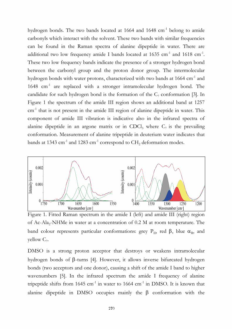
hydrogen bonds. The two bands located at 1664 and 1648 cm-1 belong to amide
carbonyls which interact with the solvent. These two bands with similar frequencies
can be found in the Raman spectra of alanine dipeptide in water. There are
additional two low frequency amide I bands located at 1635 cm-1 and 1618 cm-1.
These two low frequency bands indicate the presence of a stronger hydrogen bond
between the carbonyl group and the proton donor group. The intermolecular
hydrogen bonds with water protons, characterized with two bands at 1664 cm-1 and
1648 cm-1 are replaced with a stronger intramolecular hydrogen bond. The
candidate for such hydrogen bond is the formation of the C7 conformation [3]. In
Figure 1 the spectrum of the amide III region shows an additional band at 1257
cm-1 that is not present in the amide III region of alanine dipeptide in water. This
component of amide III vibration is indicative also in the infrared spectra of
alanine dipeptide in an argone matrix or in CDCl3 where C7 is the prevailing
conformation. Measurement of alanine tripeptide in deuterium water indicates that
bands at 1343 cm-1 and 1283 cm-1 correspond to CH2 deformation modes.
Figure 1. Fitted Raman spectrum in the amide I (left) and amide III (right) region
of Ac-Ala2-NHMe in water at a concentration of 0.2 M at room temperature. The
band colour represents particular conformations: grey PII, red , blue R, and
yellow C7.
DMSO is a strong proton acceptor that destroys or weakens intramolecular
hydrogen bonds of -turns [4]. However, it allows inverse bifurcated hydrogen
bonds (two acceptors and one donor), causing a shift of the amide I band to higher
wavenumbers [5]. In the infrared spectrum the amide I frequency of alanine
tripeptide shifts from 1645 cm-1 in water to 1664 cm-1 in DMSO. It is known that
alanine dipeptide in DMSO occupies mainly the conformation with the
270
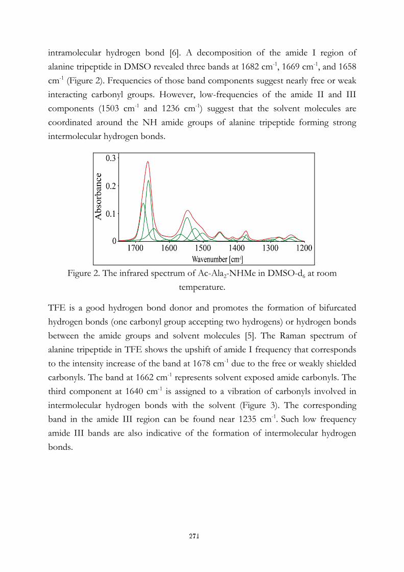
intramolecular hydrogen bond [6]. A decomposition of the amide I region of
alanine tripeptide in DMSO revealed three bands at 1682 cm-1, 1669 cm-1, and 1658
cm-1 (Figure 2). Frequencies of those band components suggest nearly free or weak
interacting carbonyl groups. However, low-frequencies of the amide II and III
components (1503 cm-1 and 1236 cm-1) suggest that the solvent molecules are
coordinated around the NH amide groups of alanine tripeptide forming strong
intermolecular hydrogen bonds.
Figure 2. The infrared spectrum of Ac-Ala2-NHMe in DMSO-d6 at room
temperature.
TFE is a good hydrogen bond donor and promotes the formation of bifurcated
hydrogen bonds (one carbonyl group accepting two hydrogens) or hydrogen bonds
between the amide groups and solvent molecules [5]. The Raman spectrum of
alanine tripeptide in TFE shows the upshift of amide I frequency that corresponds
to the intensity increase of the band at 1678 cm-1 due to the free or weakly shielded
carbonyls. The band at 1662 cm-1 represents solvent exposed amide carbonyls. The
third component at 1640 cm-1 is assigned to a vibration of carbonyls involved in
intermolecular hydrogen bonds with the solvent (Figure 3). The corresponding
band in the amide III region can be found near 1235 cm-1. Such low frequency
amide III bands are also indicative of the formation of intermolecular hydrogen
bonds.
271
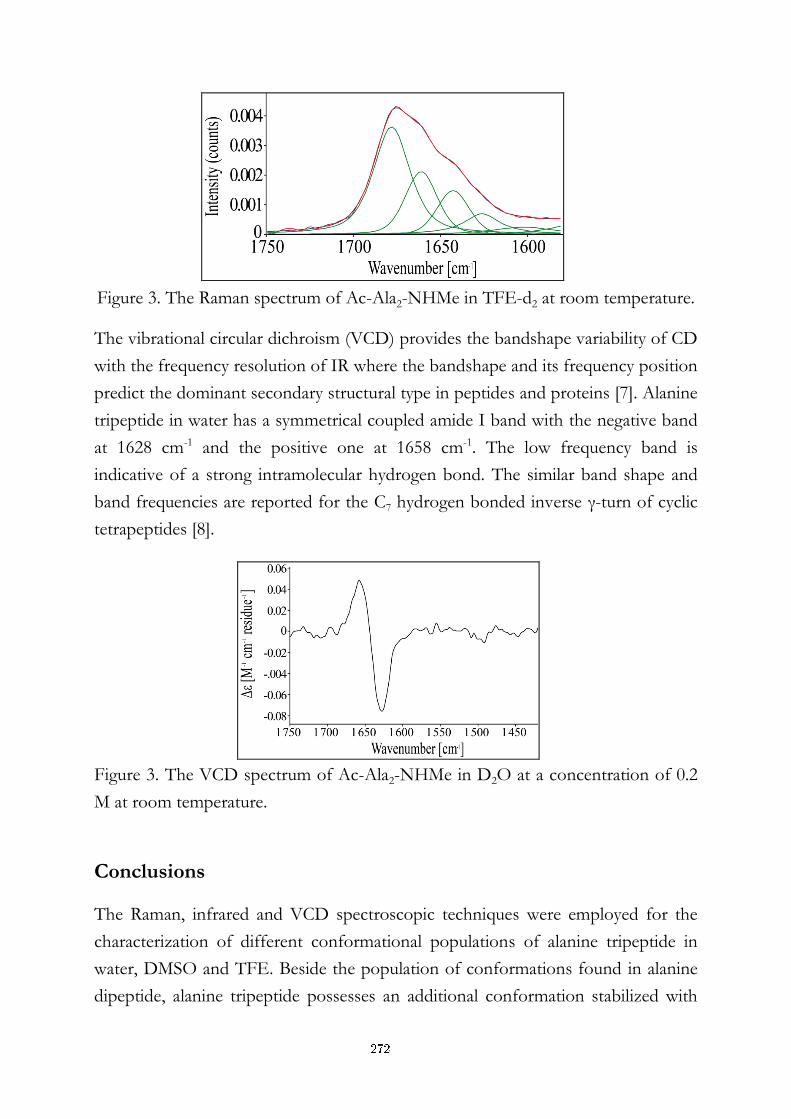
Figure 3. The Raman spectrum of Ac-Ala2-NHMe in TFE-d2 at room temperature.
The vibrational circular dichroism (VCD) provides the bandshape variability of CD
with the frequency resolution of IR where the bandshape and its frequency position
predict the dominant secondary structural type in peptides and proteins [7]. Alanine
tripeptide in water has a symmetrical coupled amide I band with the negative band
at 1628 cm-1 and the positive one at 1658 cm-1. The low frequency band is
indicative of a strong intramolecular hydrogen bond. The similar band shape and
band frequencies are reported for the C7 hydrogen bonded inverse γ-turn of cyclic
tetrapeptides [8].
Figure 3. The VCD spectrum of Ac-Ala2-NHMe in D2O at a concentration of 0.2
M at room temperature.
Conclusions
The Raman, infrared and VCD spectroscopic techniques were employed for the
characterization of different conformational populations of alanine tripeptide in
water, DMSO and TFE. Beside the population of conformations found in alanine
dipeptide, alanine tripeptide possesses an additional conformation stabilized with
272
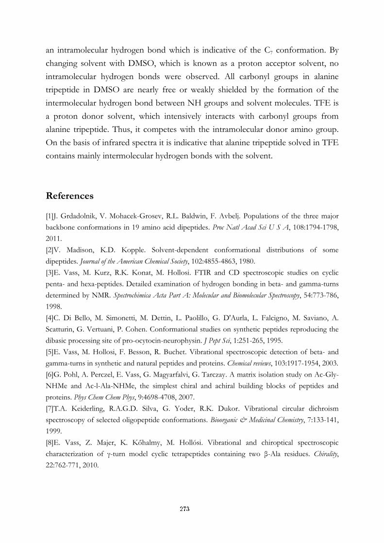
an intramolecular hydrogen bond which is indicative of the C7 conformation. By
changing solvent with DMSO, which is known as a proton acceptor solvent, no
intramolecular hydrogen bonds were observed. All carbonyl groups in alanine
tripeptide in DMSO are nearly free or weakly shielded by the formation of the
intermolecular hydrogen bond between NH groups and solvent molecules. TFE is
a proton donor solvent, which intensively interacts with carbonyl groups from
alanine tripeptide. Thus, it competes with the intramolecular donor amino group.
On the basis of infrared spectra it is indicative that alanine tripeptide solved in TFE
contains mainly intermolecular hydrogen bonds with the solvent.
References
[1]J. Grdadolnik, V. Mohacek-Grosev, R.L. Baldwin, F. Avbelj. Populations of the three major
backbone conformations in 19 amino acid dipeptides. Proc Natl Acad Sci U S A, 108:1794-1798,
2011.
[2]V. Madison, K.D. Kopple. Solvent-dependent conformational distributions of some
dipeptides. Journal of the American Chemical Society, 102:4855-4863, 1980.
[3]E. Vass, M. Kurz, R.K. Konat, M. Hollosi. FTIR and CD spectroscopic studies on cyclic
penta- and hexa-peptides. Detailed examination of hydrogen bonding in beta- and gamma-turns
determined by NMR. Spectrochimica Acta Part A: Molecular and Biomolecular Spectroscopy, 54:773-786,
1998.
[4]C. Di Bello, M. Simonetti, M. Dettin, L. Paolillo, G. D'Aurla, L. Falcigno, M. Saviano, A.
Scatturin, G. Vertuani, P. Cohen. Conformational studies on synthetic peptides reproducing the
dibasic processing site of pro-ocytocin-neurophysin. J Pept Sci, 1:251-265, 1995.
[5]E. Vass, M. Hollosi, F. Besson, R. Buchet. Vibrational spectroscopic detection of beta- and
gamma-turns in synthetic and natural peptides and proteins. Chemical reviews, 103:1917-1954, 2003.
[6]G. Pohl, A. Perczel, E. Vass, G. Magyarfalvi, G. Tarczay. A matrix isolation study on Ac-Gly-
NHMe and Ac-l-Ala-NHMe, the simplest chiral and achiral building blocks of peptides and
proteins. Phys Chem Chem Phys, 9:4698-4708, 2007.
[7]T.A. Keiderling, R.A.G.D. Silva, G. Yoder, R.K. Dukor. Vibrational circular dichroism
spectroscopy of selected oligopeptide conformations. Bioorganic & Medicinal Chemistry, 7:133-141,
1999.
[8]E. Vass, Z. Majer, K. Kőhalmy, M. Hollósi. Vibrational and chiroptical spectroscopic
characterization of γ-turn model cyclic tetrapeptides containing two β-Ala residues. Chirality,
22:762-771, 2010.
273

Za širši interes
Naše raziskovalno delo vključuje konformacijske analize kratkih peptidov, katerih
namen je razumevanje vseh sil in interakcij znotraj peptida, ki bi pomagale razumeti
začetno stopnjo proteinskega zvitja in vlogo konformacijskih preferenc aminokislin.
Ramanska in infrardeča vibracijska spektroskopija ter vibracijski cirkularni
dihroizem omogočajo natančno analizo konformacij posameznega proteina in
peptida z razčlenitvijo posameznih konformacijsko odvisnih regij v spektru.
Primerjali smo porazdelitev konformacij alanin dipeptida in alanin tripeptida v vodi.
vsebuje še znaten delež C7 konformacije, ki je stabilizirana z intramolekularno
vodikovo vezjo. Z zamenjavo topila smo pokazali, da se lahko ta vez prekine, pri
čemer molekula zavzame bolj odprto, topilu dostopnejšo strukturo.
274
Basic study of relaxors: Materials for high technological devices
Nikola Novak1,2 and Zdravko Kutnjak1,2
1 Department of Condensed Matter, Jožef Stefan Institute, Ljubljana, Slovenia
2 Jožef Stefan International Postgraduate School, Ljubljana, Slovenia
Abstract. Ferroelectric relaxors belong to a subgroup of ferroelectric
materials. Relaxors are characterised by unique dielectric, polarization,
electromechanical and electro-optical properties. These extraordinary
properties make them suitable for high technological electronic devices such as
sensors, actuators, electro or elasto-optic and photorefractive elements.
Understanding the origin of these properties and physical background is a key
for useful applications. In this paper we show the investigation of the nature
of the relaxor ground state which is one of the unresolved enigmas of relaxors.
We will interpret the high-resolution calorimetric measurements of the electric
field induced ferroelectric phase transition of the ferroelectric relaxor
Pb(Mg1/3Nb2/3)O3 single crystal oriented in the [110] direction.
Keywords: critical point, relaxor ferroelectric, latent heat.
1 Introduction
Relaxor ferroelectric materials or relaxors offer a wide range of useful properties
which make them attractive for various high technological applications. These
include ferroelectric hysteresis (used in non-volatile memories), high permittivity
(used in capacitors), high piezoelectric effects (used in sensors, actuators and
resonant wave devices such as radio-frequency filters), high pyroelectric coefficients
(used in infra-red detectors), strong electro-optic effects (used in optical switches)
and anomalous temperature coefficients of the resistivity (used in electric-motor
overload protection circuits). The largest and most important relaxor ferroelectric
family is a perovskite structured group. It was shown that the origin of relaxor
properties is due to the charge and site disorder of the perovskite structure caused
275
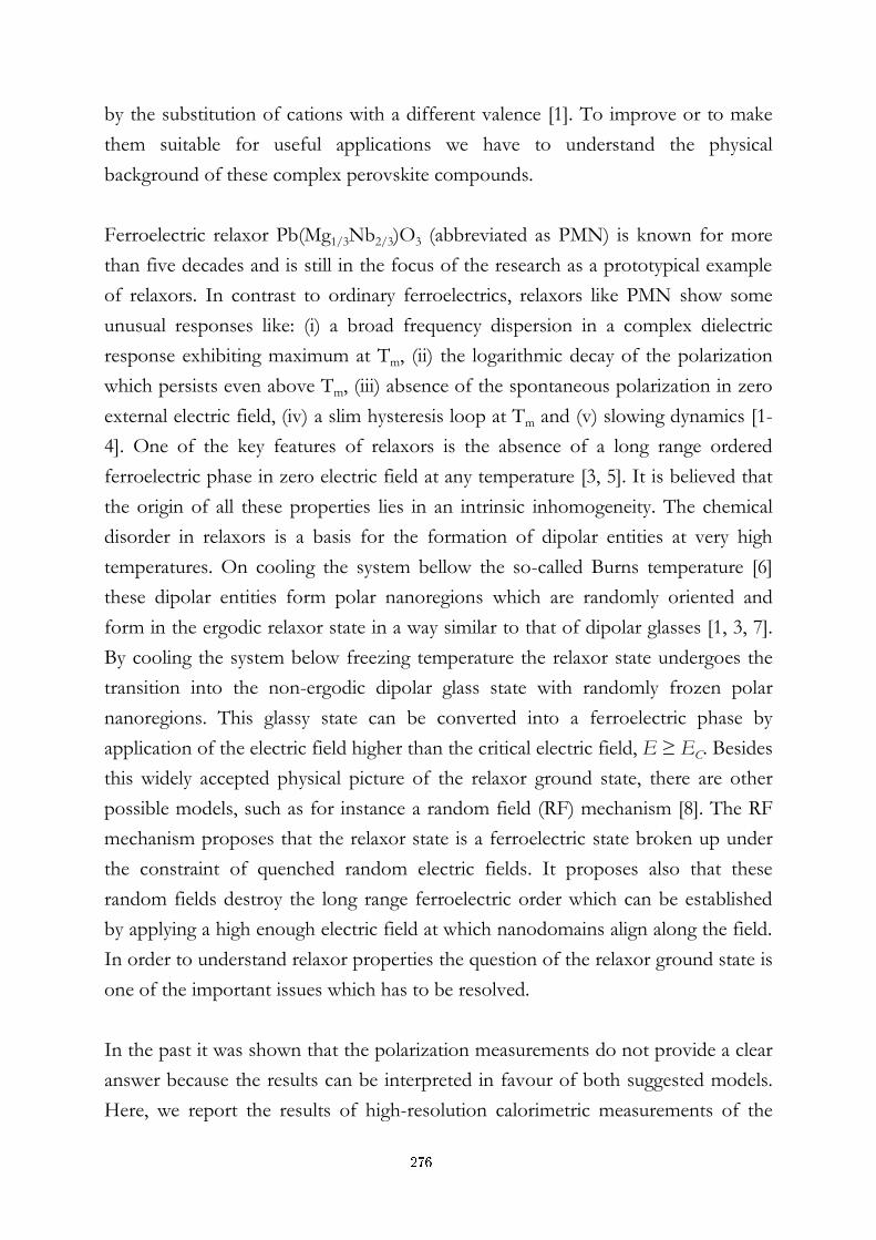
by the substitution of cations with a different valence [1]. To improve or to make
them suitable for useful applications we have to understand the physical
background of these complex perovskite compounds.
Ferroelectric relaxor Pb(Mg1/3Nb2/3)O3 (abbreviated as PMN) is known for more
than five decades and is still in the focus of the research as a prototypical example
of relaxors. In contrast to ordinary ferroelectrics, relaxors like PMN show some
unusual responses like: (i) a broad frequency dispersion in a complex dielectric
response exhibiting maximum at Tm, (ii) the logarithmic decay of the polarization
which persists even above Tm, (iii) absence of the spontaneous polarization in zero
external electric field, (iv) a slim hysteresis loop at Tm and (v) slowing dynamics [1-
4]. One of the key features of relaxors is the absence of a long range ordered
ferroelectric phase in zero electric field at any temperature [3, 5]. It is believed that
the origin of all these properties lies in an intrinsic inhomogeneity. The chemical
disorder in relaxors is a basis for the formation of dipolar entities at very high
temperatures. On cooling the system bellow the so-called Burns temperature [6]
these dipolar entities form polar nanoregions which are randomly oriented and
form in the ergodic relaxor state in a way similar to that of dipolar glasses [1, 3, 7].
By cooling the system below freezing temperature the relaxor state undergoes the
transition into the non-ergodic dipolar glass state with randomly frozen polar
nanoregions. This glassy state can be converted into a ferroelectric phase by
application of the electric field higher than the critical electric field, E ≥ EC. Besides
this widely accepted physical picture of the relaxor ground state, there are other
possible models, such as for instance a random field (RF) mechanism [8]. The RF
mechanism proposes that the relaxor state is a ferroelectric state broken up under
the constraint of quenched random electric fields. It proposes also that these
random fields destroy the long range ferroelectric order which can be established
by applying a high enough electric field at which nanodomains align along the field.
In order to understand relaxor properties the question of the relaxor ground state is
one of the important issues which has to be resolved.
In the past it was shown that the polarization measurements do not provide a clear
answer because the results can be interpreted in favour of both suggested models.
Here, we report the results of high-resolution calorimetric measurements of the
276
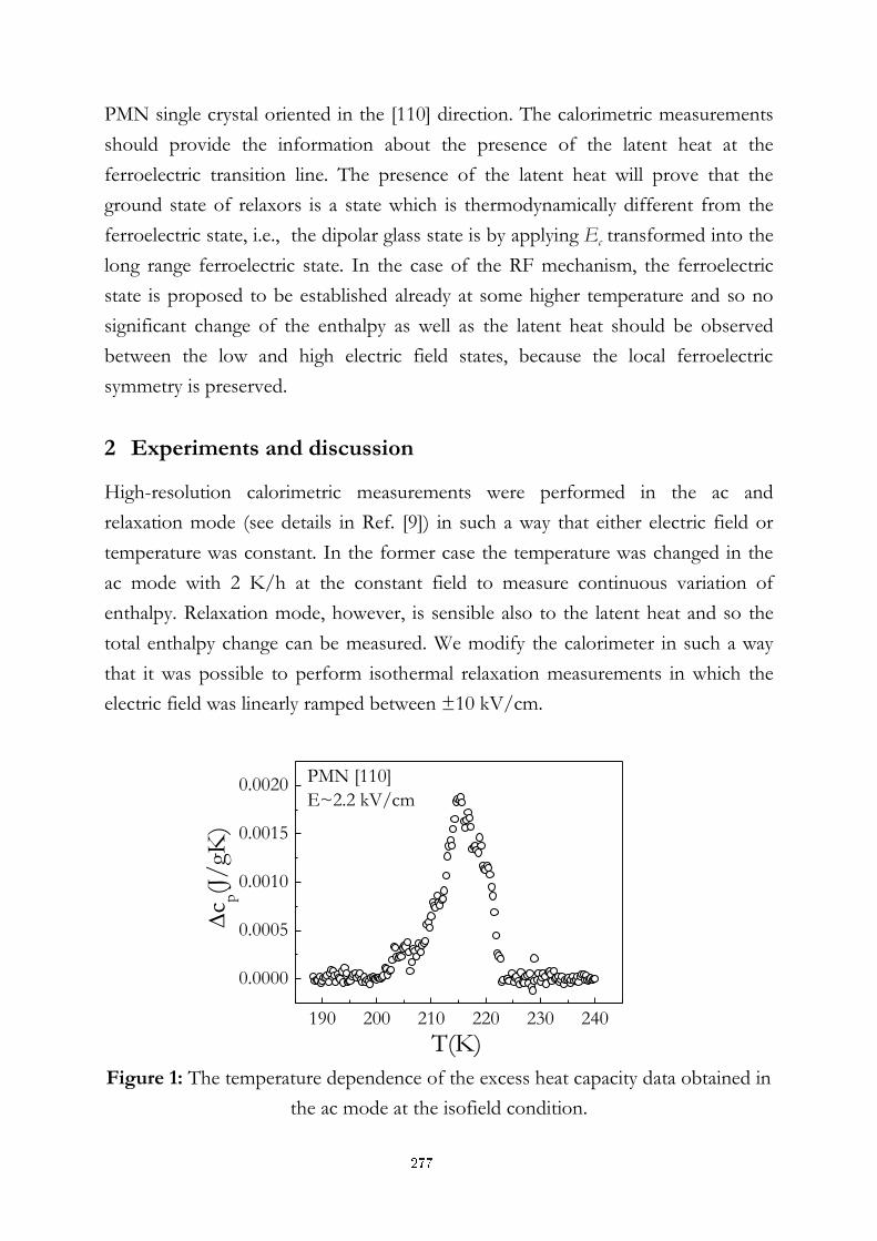
PMN single crystal oriented in the [110] direction. The calorimetric measurements
should provide the information about the presence of the latent heat at the
ferroelectric transition line. The presence of the latent heat will prove that the
ground state of relaxors is a state which is thermodynamically different from the
ferroelectric state, i.e., the dipolar glass state is by applying Ec transformed into the
long range ferroelectric state. In the case of the RF mechanism, the ferroelectric
state is proposed to be established already at some higher temperature and so no
significant change of the enthalpy as well as the latent heat should be observed
between the low and high electric field states, because the local ferroelectric
symmetry is preserved.
2 Experiments and discussion
High-resolution calorimetric measurements were performed in the ac and
relaxation mode (see details in Ref. [9]) in such a way that either electric field or
temperature was constant. In the former case the temperature was changed in the
ac mode with 2 K/h at the constant field to measure continuous variation of
enthalpy. Relaxation mode, however, is sensible also to the latent heat and so the
total enthalpy change can be measured. We modify the calorimeter in such a way
that it was possible to perform isothermal relaxation measurements in which the
electric field was linearly ramped between ±10 kV/cm.
190 200 210 220 230 240
0.0000
0.0005
0.0010
0.0015
0.0020
T(K)
c p
(J/
gK)
PMN [110]
E~2.2 kV/cm
Figure 1: The temperature dependence of the excess heat capacity data obtained in
the ac mode at the isofield condition.
277
In order to detect enthalpy changes at the ferroelectric transition the ac and
relaxation measurements of the heat capacity were conducted. The temperature
dependence of the excess heat capacity obtained from the ac measurement in PMN
[110] single crystal is displayed in Figure 1. The excess of the heat capacity can be
observed only if E ≥ EC. By increasing the electric field above 8 kV/cm, the excess
heat capacity got suppressed and smeared out. Similar behaviour of the excess heat
capacity was observed at the cubic to tetragonal (C-T) phase transition in PMN-PT
system where the first order transition line separates paraelectric cubic and
ferroelectric tetragonal phases and terminates in the critical point [10, 11].
To get a clear answer about the transition between the relaxor and ferroelectric
state in PMN we utilized modified relaxation measurements. In the isothermal
experiment we monitor the sample temperature when linearly ramped electric field
was applied. At E = EC, a sharp increase of the sample temperature was clearly
visible (see Fig. 2). The increase of the sample temperature is directly related to the
released latent heat at the electric field induced ferroelectric transition.
0 50 100 150 200 250
179.2
179.3
179.4
179.5
179.6
T(K
)
t(s)
PMN [110]
T~180 K
0 30 60 90 1200.00
0.05
0.10
0.15
0.20 T(t)=TSexp(-t/)
TS=0.2157 K
=18.423 s
T
(K)
t(s)
Figure 2: The change of the sample temperature for the PMN [110] single crystal
as a consequence of the released latent heat at the field induced ferroelectric
transition, at 180 K. The inset shows a fit to the simple exponential decay ansatz
which reveals the amplitude of the sample temperature change and thus the latent
heat.
278
To determinate the released latent heat in the first approximation we fit the
dissipated latent heat into the surrounding by the simple exponential decay ansatz
as shown in the inset of Fig. 2. The obtained amplitude of the sample temperature
change, ΔTS=0.2157 K, can be used to calculate corresponding latent heat. With
further measurements it was shown that the amplitude of the sample temperature
change decreases with increasing temperature and electric field. The presence and
diminishing of the latent heat prove the existence of the first order transition line
between the relaxor and ferroelectric phases which terminates at the critical point.
3 Conclusion
High-resolution heat capacity measurements were employed to investigate the
nature of the electric field induced ferroelectric transition of the ferroelectric
relaxor PMN single crystal oriented in [110]. The ac measurements display an
excess of the heat capacity at E ≥ EC. At a much higher electric field the heat
capacity anomaly is suppressed indicating the supercritical behaviour. The detected
latent heat confirms the existence of a real phase transition line between the zero-
field ground state and ferroelectric long range order. The calorimetric
measurements reveal a similar behaviour as observed at the C-T phase transition in
the PMN-PT system. The presence of the latent heat supports the idea of the
dipolar glass like ground state of relaxors rather than the RF frozen ferroelectric
state broken up into nanodomains.
References:
[1] L. E. Cross. Relaxor ferroelectrics. Ferroelectrics, 76:241-267, 1987. [2] D. Viehland, S. J. Jang, L. E. Cross, M. Wuttig. Deviation from Curie-Weiss behaviour in
relaxor ferroelectrics. Physical Review B, 46:8003, 1992. [3] V. E. Colla, E. Y. Koroleva, N. M. Okuneva, S. B. Vakhrushev. Long-Time Relaxation of the
Dielectric Response in Lead Magnoniobate. Physiscal Review Letters, 74:1681, 1995. [4] A. Levstik, Z. Kutnjak, C. Filipič, R. Pirc. Glassy freezing in relaxor ferroelectric lead
magnesium niobate. Physical Review B, 57:11204, 1998. [5] G. Schmidt, H. Arndt, G. Borchhardt, J. von Cieminski, T. Petzsche, K. Borman, A.
Sternberg, A. Zirnite, V. A. Isupov. Induced Phase Transitions in Ferroelectrics with Diffuse Phase Transition. Physica Status Solid, 63:501, 1981.
[6] G. Burns, F. H. Dacol. Crystalline ferroelectrics with glassy polarization behavior. Physical Review B 28:2527, 1983.
[7] R. Pirc, R. Blinc. Spherical random-bond-random-field model of relaxor ferroelectrics. Physical Review B, 60:13470, 1999.
279

[8] V. Westphal, W. Kleemann, M. D. Glinchuk. Diffuse Phase Transition and Random-Field-Induced Domain States of the “Relaxor” Ferroelectric PbMg1/3Nb2/3O3. Physical Review Letters, 68:847, 1992.
[9] H. Yao, K. Ema, C.W. Garland. Nonadiabatic scanning calorimeter. Review of Scientific Instruments, 69:172, 1998.
[10] Z. Kutnjak, J. Petzelt, R. Blinc. The giant electromechanical response in ferroelectric relaxors as a critical phenomenon. Nature, 441:956-959, 2006.
[11] Z. Kutnjak, R. Blinc, Y. Ishibashi. Electric field induced critical points and polarization rotations in relaxor ferroelectrics. Physical Review B, 76:104102,2007.
280
For wider interest
Relaxor ferroelectric materials represent a subgroup of ferroelectrics.
Pb(Mg1/3Nb2/3)O3 is one of the most famous and widely studied relaxor. Relaxor
materials are known for their unusual properties which are useful for various
applications in high technological devices. Relaxors exhibit high permittivity
(used in capacitors), ferroelectric hysteresis (used in non-volatile memories), high
piezoelectric effects (used in sensors, actuators and resonant wave devices such
as the radio-frequency filters, scanning probe microscopy, ink jet printer,
adaptive optics, micromotors, vibration sensors/attenuators, Hubble telescope
correction), high pyroelectric coefficients (used in infra-red detectors), strong
electro-optic effects (used in optical switches, segmented displays, modulators,
image storage, holographic data storage) and anomalous temperature coefficients
of the resistivity (used in electric-motor overload protection circuits). Our work
is dedicated to understanding the ordering process in this material which is of a
fundamental importance for the further application progress as well as
engineering new materials with enhanced properties.
In this work we represent the study of the glass-ferroelectric phase transition
that addresses also the long standing question about the ground state of relaxors
in zero electric field. The isofield and isothermal measurements of the heat
capacity reveal an excess of the heat capacity as well as released latent heat at the
field induced ferroelectric transition. The detected latent heat confirms the
existence of the real ferroelectric phase transition and support the physical
picture of the dipolar glass like ground state of relaxors.
281
Morfotropna fazna meja v (Na1-xKx)0,5Bi0,5TiO3 piezoelektrični keramiki
Mojca Otoničar1,2
1 Odsek za raziskave sodobnih materialov, Institut Jožef Stefan, Ljubljana, Slovenija 2 Mednarodna podiplomska šola Jožefa Stefana, Ljubljana, Slovenija
Mentor: doc. dr. Srečo D. Škapin
Razvoj piezoelektrikov je pretežno usmerjen v optimizacijo strukture materialov, saj so v območju morfotropne fazne meje (MPB) piezoelektrični odzivi občutno povišani. Keramikam na osnovi sistema (Na1-xKx)0,5Bi0,5TiO3, kjer se tvori trdna topnost v območju sestav 0 ≤ x ≤ 1, sem določila strukturne značilnosti in izvedla meritve elektromehanskih lastnosti. Določila sem sestave z MPB (pri x = 0,2 in 0,22), kjer soobstojata romboedrična in tetragonalna struktura. Prisotnost MPB potrjujejo tudi rezultati električnih meritev; vzorec s sestavo x = 0,2 izkazuje najvišje vrednosti dielektrične konstante, remanentne polarizacije in piezoelektričnega koeficienta. Analiza s presevnim elektronskim mikroskopom (TEM) je pokazala, da v MPB prevladuje tetragonalna domenska zgradba, superstrukturni ukloni v elektronskih difrakcijah pa potrjujejo obstoj P4bm tetragonalne strukture. Rezultati TEM analize ne sovpadajo z rezultati rentgenske praškovne difrakcije (RTG), ki pri sestavi x = 0,2 kažejo pretežno romboedrično strukturo. In-situ TEM meritve s segrevanjem do 500°C so potrdile, da se po ohlajanju tetragonalna domenska zgradba ne vzpostavi ponovno. Tako lahko sklepamo, da je tetragonalna struktura sprožena z mehanskim obremenjevanjem med pripravo vzorcev za TEM, kar ustreza visoki polarizabilnosti ter strukturni 'prilagodljivosti' MPB materialov.
Ključne besede: piezoelektrik, morfotropna fazna meja, presevna elektronska
mikroskopija (TEM)
1 Uvod
Piezoelektrični materiali se uporabljajo kot sestavne komponente predvsem v
elektronski industriji kot senzorji, pretvorniki ali aktuatorji. Tako različne naprave
izkoriščajo piezoelektrično lastnost materialov, da se polarizirajo oziroma
deformirajo pod vplivom električnega polja, ali da generirajo električno napetost
kot posledico mehanske obremenitve. Težnja pri razvoju novih piezoelektričnih
materialov je v izboljšanju piezoelektričnega odziva, kar prispeva k izboljšavi
učinkovitosti komponent in k miniaturizaciji elektronskih naprav. Zato je študij
poteka sprememb v materialu, kot na primer spremembe strukture zaradi sestave ali 282
zaradi sekundarno vnesenih napetosti pri obremenitvah materiala, ali pa premikanje
domenskih sten pod vplivom polja, izrednega pomena za nadaljnji razvoj
piezomaterialov.
Najpogosteje uporabljeni piezoelektrični materiali vsebujejo svinec (PbZrxTi1-xO3),
ki je strupen tako za človeka kot za okolje. Zato je cilj razvoja novih
piezomaterialov priprava materialov brez ali z manj vsebnosti svinca. Med
najprimernejše piezomateriale, ki bi potencialno lahko zamenjali materiale na
osnovi svinca, sodijo sistemi trdnih raztopin s perovskitno strukturo v območju
morfotropne fazne meje (MPB), kjer soobstojata dve različni strukturi. [1-6] V tem
območju namreč piezoelektrični materiali izkazujejo močnejšo elektromehansko
sklopitev in s tem povišane vrednosti piezoelektričnega odziva. [1,2]
Na podlagi predhodnih študij smo se odločili za raziskave keramik iz sistema
Na0,5Bi0,5TiO3-K0,5Bi0,5TiO3 (NBT-KBT), ki v določenem razmerju kationov tvorijo
MPB med tetragonalno in romboedrično strukturo. Tako sem določila sestavo, pri
kateri se pojavlja MPB, ovrednotila elektromehanske lastnosti trdnih raztopin in
podrobno analizirala kristalno in domensko strukturo keramik.
2 Eksperimentalni del
Keramične vzorce v obliki trdnih raztopin z različnimi deleži NBT in KBT sem
pripravila po postopku sinteze v trdnem. Fazno sestavo in kristaliničnost vzorcev
sem preverila z rentgensko praškovno difrakcijo (RTG) s pomočjo difraktometra
Bruker AXS D4 Endeavor. Za detajlne raziskave lokalne kristalne in domenske
strukture sem vzorce v obliki tanke folije analizirala s presevnim elektronskim
mikroskopom (TEM; JEM-2100, Jeol Ltd., Tokyo, Japan).
3 Rezultati in diskusija
3.1 Rentgenska praškovna difrakcija (RTG)
Z rentgensko praškovno difrakcijo sem določila kristalno strukturo trdnih raztopin
NBT-KBT. Iz difraktogramov je razvidno, da se lege posameznih uklonov zvezno
zamaknejo s spreminjajočo se sestavo, kar sovpada z večanjem osnovne celice od
NBT proti KBT. Natančni RTG posnetki sestav x = 0,2 in 0,22 v (Na1-
283
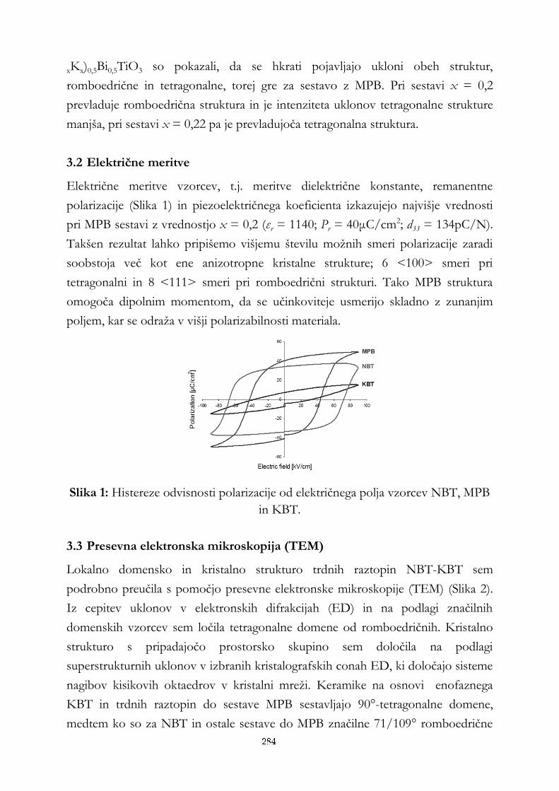
xKx)0,5Bi0,5TiO3 so pokazali, da se hkrati pojavljajo ukloni obeh struktur,
romboedrične in tetragonalne, torej gre za sestavo z MPB. Pri sestavi x = 0,2
prevladuje romboedrična struktura in je intenziteta uklonov tetragonalne strukture
manjša, pri sestavi x = 0,22 pa je prevladujoča tetragonalna struktura.
3.2 Električne meritve
Električne meritve vzorcev, t.j. meritve dielektrične konstante, remanentne
polarizacije (Slika 1) in piezoelektričnega koeficienta izkazujejo najvišje vrednosti
pri MPB sestavi z vrednostjo x = 0,2 (εr = 1140; Pr = 40μC/cm2; d33 = 134pC/N).
Takšen rezultat lahko pripišemo višjemu številu možnih smeri polarizacije zaradi
soobstoja več kot ene anizotropne kristalne strukture; 6 <100> smeri pri
tetragonalni in 8 <111> smeri pri romboedrični strukturi. Tako MPB struktura
omogoča dipolnim momentom, da se učinkoviteje usmerijo skladno z zunanjim
poljem, kar se odraža v višji polarizabilnosti materiala.
Slika 1: Histereze odvisnosti polarizacije od električnega polja vzorcev NBT, MPB
in KBT.
3.3 Presevna elektronska mikroskopija (TEM)
Lokalno domensko in kristalno strukturo trdnih raztopin NBT-KBT sem
podrobno preučila s pomočjo presevne elektronske mikroskopije (TEM) (Slika 2).
Iz cepitev uklonov v elektronskih difrakcijah (ED) in na podlagi značilnih
domenskih vzorcev sem ločila tetragonalne domene od romboedričnih. Kristalno
strukturo s pripadajočo prostorsko skupino sem določila na podlagi
superstrukturnih uklonov v izbranih kristalografskih conah ED, ki določajo sisteme
nagibov kisikovih oktaedrov v kristalni mreži. Keramike na osnovi enofaznega
KBT in trdnih raztopin do sestave MPB sestavljajo 90°-tetragonalne domene,
medtem ko so za NBT in ostale sestave do MPB značilne 71/109° romboedrične
284
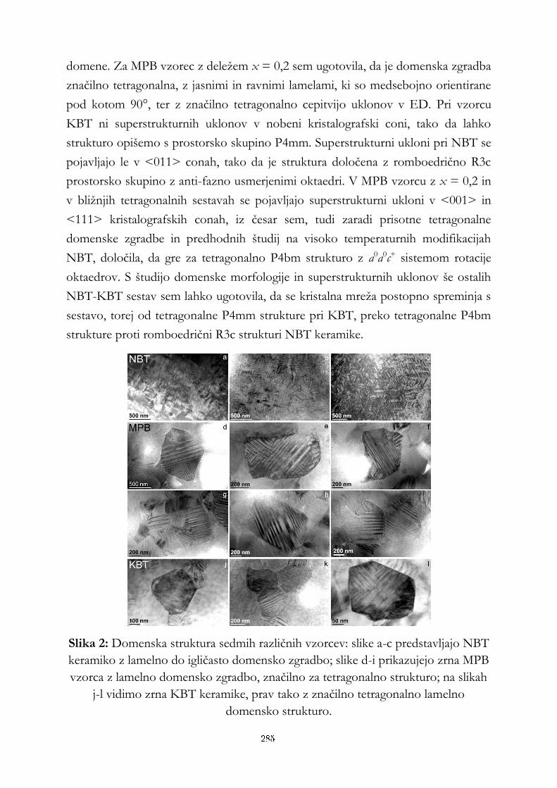
domene. Za MPB vzorec z deležem x = 0,2 sem ugotovila, da je domenska zgradba
značilno tetragonalna, z jasnimi in ravnimi lamelami, ki so medsebojno orientirane
pod kotom 90°, ter z značilno tetragonalno cepitvijo uklonov v ED. Pri vzorcu
KBT ni superstrukturnih uklonov v nobeni kristalografski coni, tako da lahko
strukturo opišemo s prostorsko skupino P4mm. Superstrukturni ukloni pri NBT se
pojavljajo le v <011> conah, tako da je struktura določena z romboedrično R3c
prostorsko skupino z anti-fazno usmerjenimi oktaedri. V MPB vzorcu z x = 0,2 in
v bližnjih tetragonalnih sestavah se pojavljajo superstrukturni ukloni v <001> in
<111> kristalografskih conah, iz česar sem, tudi zaradi prisotne tetragonalne
domenske zgradbe in predhodnih študij na visoko temperaturnih modifikacijah
NBT, določila, da gre za tetragonalno P4bm strukturo z a0a0c+ sistemom rotacije
oktaedrov. S študijo domenske morfologije in superstrukturnih uklonov še ostalih
NBT-KBT sestav sem lahko ugotovila, da se kristalna mreža postopno spreminja s
sestavo, torej od tetragonalne P4mm strukture pri KBT, preko tetragonalne P4bm
strukture proti romboedrični R3c strukturi NBT keramike.
Slika 2: Domenska struktura sedmih različnih vzorcev: slike a-c predstavljajo NBT
keramiko z lamelno do igličasto domensko zgradbo; slike d-i prikazujejo zrna MPB
vzorca z lamelno domensko zgradbo, značilno za tetragonalno strukturo; na slikah
j-l vidimo zrna KBT keramike, prav tako z značilno tetragonalno lamelno
domensko strukturo.
285
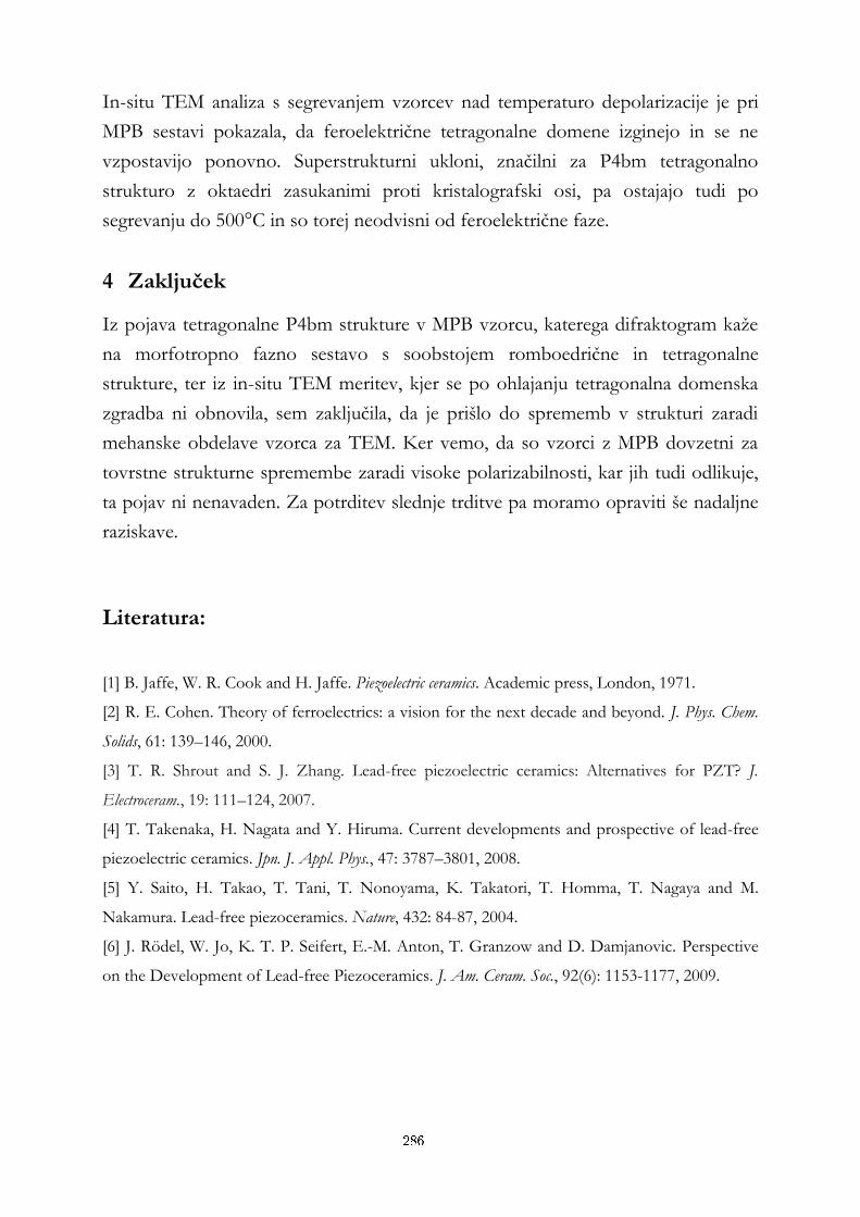
In-situ TEM analiza s segrevanjem vzorcev nad temperaturo depolarizacije je pri
MPB sestavi pokazala, da feroelektrične tetragonalne domene izginejo in se ne
vzpostavijo ponovno. Superstrukturni ukloni, značilni za P4bm tetragonalno
strukturo z oktaedri zasukanimi proti kristalografski osi, pa ostajajo tudi po
segrevanju do 500°C in so torej neodvisni od feroelektrične faze.
4 Zaključek
Iz pojava tetragonalne P4bm strukture v MPB vzorcu, katerega difraktogram kaže
na morfotropno fazno sestavo s soobstojem romboedrične in tetragonalne
strukture, ter iz in-situ TEM meritev, kjer se po ohlajanju tetragonalna domenska
zgradba ni obnovila, sem zaključila, da je prišlo do sprememb v strukturi zaradi
mehanske obdelave vzorca za TEM. Ker vemo, da so vzorci z MPB dovzetni za
tovrstne strukturne spremembe zaradi visoke polarizabilnosti, kar jih tudi odlikuje,
ta pojav ni nenavaden. Za potrditev slednje trditve pa moramo opraviti še nadaljne
raziskave.
Literatura:
[1] B. Jaffe, W. R. Cook and H. Jaffe. Piezoelectric ceramics. Academic press, London, 1971.
[2] R. E. Cohen. Theory of ferroelectrics: a vision for the next decade and beyond. J. Phys. Chem.
Solids, 61: 139–146, 2000.
[3] T. R. Shrout and S. J. Zhang. Lead-free piezoelectric ceramics: Alternatives for PZT? J.
Electroceram., 19: 111–124, 2007.
[4] T. Takenaka, H. Nagata and Y. Hiruma. Current developments and prospective of lead-free
piezoelectric ceramics. Jpn. J. Appl. Phys., 47: 3787–3801, 2008.
[5] Y. Saito, H. Takao, T. Tani, T. Nonoyama, K. Takatori, T. Homma, T. Nagaya and M.
Nakamura. Lead-free piezoceramics. Nature, 432: 84-87, 2004.
[6] J. Rödel, W. Jo, K. T. P. Seifert, E.-M. Anton, T. Granzow and D. Damjanovic. Perspective
on the Development of Lead-free Piezoceramics. J. Am. Ceram. Soc., 92(6): 1153-1177, 2009.
286

Za širši interes
Novi piezoelektrični materiali brez vsebnosti svinca, ki v določenem območju
sestav izkazujejo močno povišane vrednosti elektromehanske sklopitve, se
raziskujejo zaradi njihove potencialne uporabe v elektroniki. Pri trdnih raztopinah s
povišanimi piezoelektričnimi lastnostmi se namreč pojavi soobstoj dveh kristalnih
struktur – območje imenujemo morfotropna fazna meja - zaradi česar se material
enostavneje polarizira. Dejansko stanje kristalne strukture MPB je težko
ovrednotiti, saj so metode ugotavljanja strukture posredne, povprečne ali invazivne,
kar botruje številnim nesoglasjem stroke o realnem stanju strukture materiala. Naše
raziskave so potekale na sistemu trdnih raztopin (Na1-xKx)0,5Bi0,5TiO3, za katere smo
določili strukturne in električne lastnosti piezokeramik. Detajlne analize kristalne in
domenske zgradbe so potekale s pomočjo presevne elektronske mikroskopije v
kombinaciji z rentgensko praškovno difrakcijo.
287

The peak base as a characteristic feature of the Auger electron spectra
Besnik Poniku1,2, Igor Belič1, Monika Jenko1
1 Institute of Metals and Technology, Ljubljana, Slovenia
2 Jožef Stefan International Postgraduate School, Ljubljana, Slovenia
Abstract. The background in Auger spectra has always been regarded as
nuisance. Its removal presents a real challenge when processing data from
Auger spectra in order to extract from them the required information. This
task becomes even more immediate and unavoidable when one thinks of
automating the retrieval of qualitative and quantitative information from the
Auger spectra. For this reason different approaches have been developed from
various researchers to overcome this problem. On the other hand we should
not disregard the fact that the background also carries information. For this
reason the removed background should be saved for reference when
necessary.
Keywords: Auger spectra, automation, background, peak base.
1 Introduction
Ideally, when recording Auger spectra, we should see on the plot only the
characteristic peaks coming from the elements present in the sample. In such a case
the intensity represented by the area under the peaks would be strictly defined. But
when obtaining real spectra from samples the characteristic peaks are always
situated on a top of the background [1].
2 Contributors to the background
The signal that forms the background of the Auger spectra is generated from three
principal sources: the backscattered electrons, the secondary electrons, and the
inelastically scattered Auger electrons [2]. The backscattered electrons are electrons
of the primary beam which come back at the surface of the sample and reach the
288

detector after having penetrated the sample. Authors like Jousset and Langeron [3]
worked on defining the inelastically scattered primary electron spectrum. They
proposed a model which predicts in a wide energy range, from about 0.2 to 0.75 Ep
(energy of the primary beam), an exponential law for the contribution of
backscattered primary electrons to the spectrum in the integral form [the N(E)
spectrum]. Equation (1) [2] gives the relationship in a simplified form:
)/exp()( 1EEEnB , (1)
where nB represents the number of backscattered primary electrons leaving the
surface at energies E, whereas E1 corresponds to a minimum loss which is a fixed
value for a certain energy of the primary beam.
Secondary electrons are considered in general as those electrons which are created
as a result of the primary beam electrons interaction with the sample. Sickafus’
work describes the contribution of the secondary electrons to the spectrum [4, 5].
The contribution of the secondary electrons could be written as [6]:
,)( mAEEB (2)
where B(E) is the number distribution of secondary electrons emitted with the
kinetic energy E from a solid sample, A and m are constants characteristic of the
material, but A also depends upon the energy of the primary beam.
Sickafus also studied the Auger emission from the sample, describing it in two
parts, namely as the elastic Auger emission coming from the surface, and the
scattered Auger emission coming from the subsurface of the sample (Fig. 1) [4, 5].
Figure 1: Emissions from the surface and subsurface and their effect on the
spectrum.[5]
289
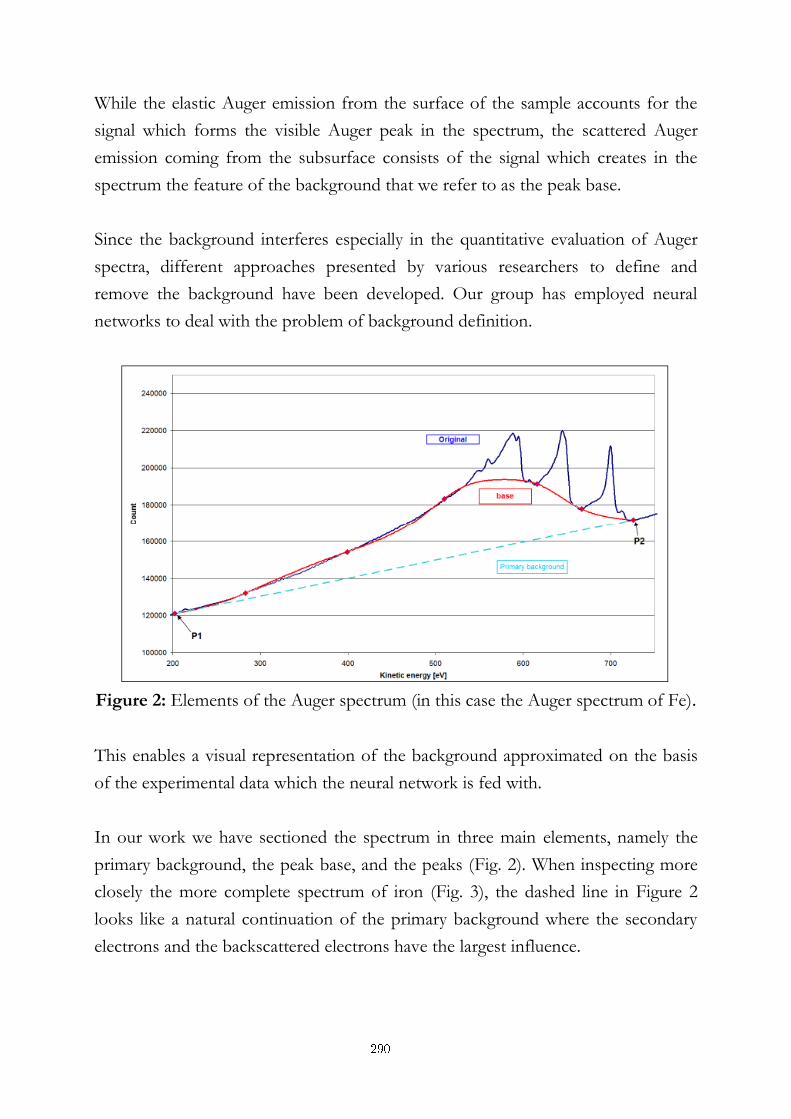
While the elastic Auger emission from the surface of the sample accounts for the
signal which forms the visible Auger peak in the spectrum, the scattered Auger
emission coming from the subsurface consists of the signal which creates in the
spectrum the feature of the background that we refer to as the peak base.
Since the background interferes especially in the quantitative evaluation of Auger
spectra, different approaches presented by various researchers to define and
remove the background have been developed. Our group has employed neural
networks to deal with the problem of background definition.
Figure 2: Elements of the Auger spectrum (in this case the Auger spectrum of Fe).
This enables a visual representation of the background approximated on the basis
of the experimental data which the neural network is fed with.
In our work we have sectioned the spectrum in three main elements, namely the
primary background, the peak base, and the peaks (Fig. 2). When inspecting more
closely the more complete spectrum of iron (Fig. 3), the dashed line in Figure 2
looks like a natural continuation of the primary background where the secondary
electrons and the backscattered electrons have the largest influence.
290
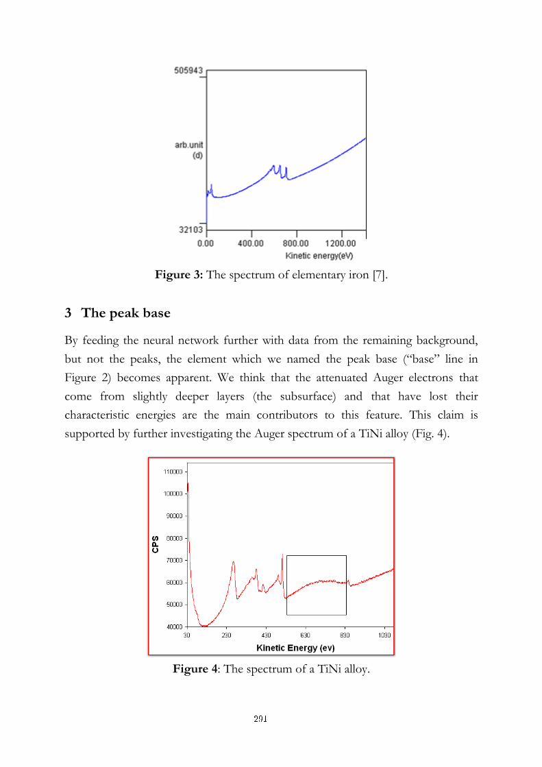
Figure 3: The spectrum of elementary iron [7].
3 The peak base
By feeding the neural network further with data from the remaining background,
but not the peaks, the element which we named the peak base (“base” line in
Figure 2) becomes apparent. We think that the attenuated Auger electrons that
come from slightly deeper layers (the subsurface) and that have lost their
characteristic energies are the main contributors to this feature. This claim is
supported by further investigating the Auger spectrum of a TiNi alloy (Fig. 4).
Figure 4: The spectrum of a TiNi alloy.
291
In this case the Ni was slightly buried under the Ti oxide that was formed on the
surface and the contaminating carbon, whose peaks (Ti, O, and C) are clearly
observable in the spectrum. Therefore, the signal coming from Ni was slightly
attenuated, and instead of clear peaks in the area encompassed by the square in
Figure 4 we observe a “bump”. From the knowledge of the sample used in this
case, and the energy interval where this feature appears, we come to the conclusion
that it is largely influenced by the Auger signal of Ni present in the subsurface.
Since it is very obvious that this feature very much resembles the peak base
described in Figure 2, we also come to the conclusion that the part of the
background under the respective peaks comes as a result of the attenuation of the
Auger electrons which are generated in the subsurface.
In instances like the one presented in Figure 4, where the signal is not strong
enough to form clear peaks, the peak base feature of the background may be used
to detect the presence of the element in question. This fact that the background
may contain information regarding the investigated sample should be kept in mind
during the background removal operations, and the removed background should
be saved for reference if necessary.
References:
[1] Auger Electron Spectroscopy. Queen Mary, University of London.
http://www.chem.qmul.ac.uk/surfaces/scc/scat5_2.htm, 2012.
[2] M.P. Seah, I. S. Glimore. High Resolution Digital Auger Database of true spectra for Auger
elenctron spectroscopy intensities. Journal of Vacuum Science and Technology A, 14(3): 1401-1407,
1996.
[3] D. Jousset, J. P. Langeron. Energy distribution of primary backscattered electrons in Auger
electron spectroscopy. Journal of Vacuum Science and Technology A, 5(4): 989-995, 1987.
[4] E. N. Sickafus. Linearized secondary – electron cascades from the surfaces of metals. I. Clean
surfaces of homogeneous specimens. Physical Review B, 16(4): 1436-1447, 1977.
[5] E. N. Sickafus. Linearized secondary – electron cascades from the surfaces of metals. II.
Surface and subsurface sources. Physical Review B, 16(4): 1448-1458, 1977.
[6] J. C. Greenwood, M. Prutton, and R. H. Roberts. Atomic – number dependence of the
secondary – electron cascade from solids. Physical Review B, 49(18):12485-12495, 1994.
[7] COMPRO 10 - Common Data Processing System Version 10.
http://www.sasj.jp/COMPRO/, 2012.
292
For wider interest
The long term goal of our group is to automate the interpretation of spectra in
Auger Electron Spectroscopy. To automate the interpretation of the quantitative
and qualitative results obtained from the Auger spectra, in other words to enable
the software to automatically tell us which elements are present in the surface of
the sample and how much of each element is there, among other things, we must
prepare the data by removing the background. The background interferes when we
attempt to analyze how much of a specific element is presented in the sample.
Even though the idea is straightforward, simply just to remove the background, the
actual work of its removal is quite a challenge. Different researchers have taken
different approaches to overcome the problem of how to define the background
for its later proper removal. Our group has used neural networks for this purpose,
modelling the background by feeding the neural network with the data that were
obtained experimentally.
By visually inspecting the different approximated (modelled) parts of the
background, a feature which we termed “the peak base” became apparent. We
investigated further and found out that most of the researchers in the previous
work on the topic of background definition and its later removal had treated this as
an integral part of the feature that we termed “the primary background”. But unlike
the primary background, the peak base is actually formed from characteristic Auger
electrons which normally would form the main peak, but are slowed down and lose
slightly their characteristic energy since the electrons forming the peak base are
generated deeper in the sample surface (the subsurface) and thus travel further and
overcome additional obstacles on their way to the detector. Thus, the background
that would normally be removed and hence its signal would be lost, actually carries
information about our sample and can be used to detect elements when clear peaks
are absent.
Through this work we attempt to bring the automation of Auger spectra
interpretation one step closer. This on the one hand will make the analysis much
easier for anyone involved in the study of metals and other materials through
Auger spectroscopy, and on the other hand the proposed advanced treatment of
the background part of Auger spectra will contribute to more reliable results about
the elements present in the samples studied.
293
Underwater electromagnetic remote sensing
Uroš Puc1, Andreja Abina1, Anton Jeglič3, Pavel Cevc2, Aleksander
Zidanšek1,2
1 Jožef Stefan International Postgraduate School, Ljubljana, Slovenia
2 Department of Condensed Matter Physics, Jožef Stefan Institute, Ljubljana,
Slovenia
3 Faculty of Electical Engineering, University of Ljubljana, Tržaška 14, Ljubljana,
Slovenia
Abstract
Utilization of non-destructive and non-invasive methods for the real-time underwater
remote sensing is one of the challenging and desired tasks in the maritime security
and safety as well as the harbour surveillance. Our aim was to develop and verify
advanced electromagnetic sensors for a seabed objects detection and inspection. The
seabed is a complex environment often covered with the sand, dense aquatic
vegetation and rocks. Hence, it is difficult to investigate the seabed by only one
conventional method. Usually a combination of the sonar and video system is used
for the detection and classification of underwater targets. In this paper, we verified
the operation and efficiency of two EM imaging sensors, a ground penetrating radar
(GPR) and an electromagnetic continuous wave sensor (CWEMS).
Keywords: electromagnetic sensors, GPR, remote sensing, underwater
detection.
1 Introduction
The underwater remote sensing technology plays a key role in investigations of the
underwater environment and detection of unknown objects. Nowadays, several
techniques (Fig. 1) exist in this field; the most important among them are acoustic,
electromagnetic and optical devices [1-6]. Electromagnetic (EM) sensors have long
been recognized as a useful tool for the geophysical exploration and remote
sensing. However, no system currently available on the market is capable to
accurately survey and map the location of objects buried under the bottom
294
sediments or vegetation. The technology that we selected includes an adapted
version of the ground penetrating radar (GPR) and the continuous wave
electromagnetic sensor (CWEMS) which are competing tools against the SONAR
(sound navigation and ranging) and metal detector. The preliminary results
achieved by these two EM sensing methods are presented in this paper.
2 EM sensing methods
The EM propagation in water is very different from the propagation through air
due to the high permittivity and electrical conductivity of water. In freshwater the
conductivity is 0.1 - 10 mS/m, whereas in sea water this value is around 4 S/m.
Another difference is a greater attenuation loss of the propagation pulses in water.
It depends on the selected frequency and salinity of water. Hence, for the
freshwater and sea water the attenuation loss at 100 MHz is 0.1 dBm-1 and 100
dBm-1, respectively, whereas at 1 GHz it increases to 1 dBm-1 and 1000 dBm-1,
respectively. Furthermore, the propagation velocity and corresponding wavelength
in water decrease by a factor of about 10 in comparison to the velocity and
wavelength in air [1-3].
1.1 Ground penetrating radar
The ground penetrating radar or GPR is a non-destructive geophysical method
based on the propagation of high frequency electromagnetic waves. The GPR
method images structures in the ground that are related to changes in the dielectric
properties [1]. If a very short EM pulse is transmitted by an electric dipole into the
medium, it propagates in the subsurface with a velocity depending on the electrical
properties of the medium. For a layered subsurface with contrasting electrical
properties, a part of the EM energy is reflected back to the surface where it is
detected by a receiver dipole and recorded. Synchronization between the
transmitter and the receiver systems allows the determination of the time taken for
the EM pulse to be reflected back. In our case, several candidate sites were
surveyed to find out a test area with the desired water depth for the underwater
GPR investigation. We selected the lake Podpeč, a location near the city of
Ljubljana. The lake is located in the Karst region and it is the deepest lake in
Slovenia with a depth of 47 m. The experimental work was conducted using a
commercial GPR system equipped with a 250 MHz and 50 MHz antenna. The
295
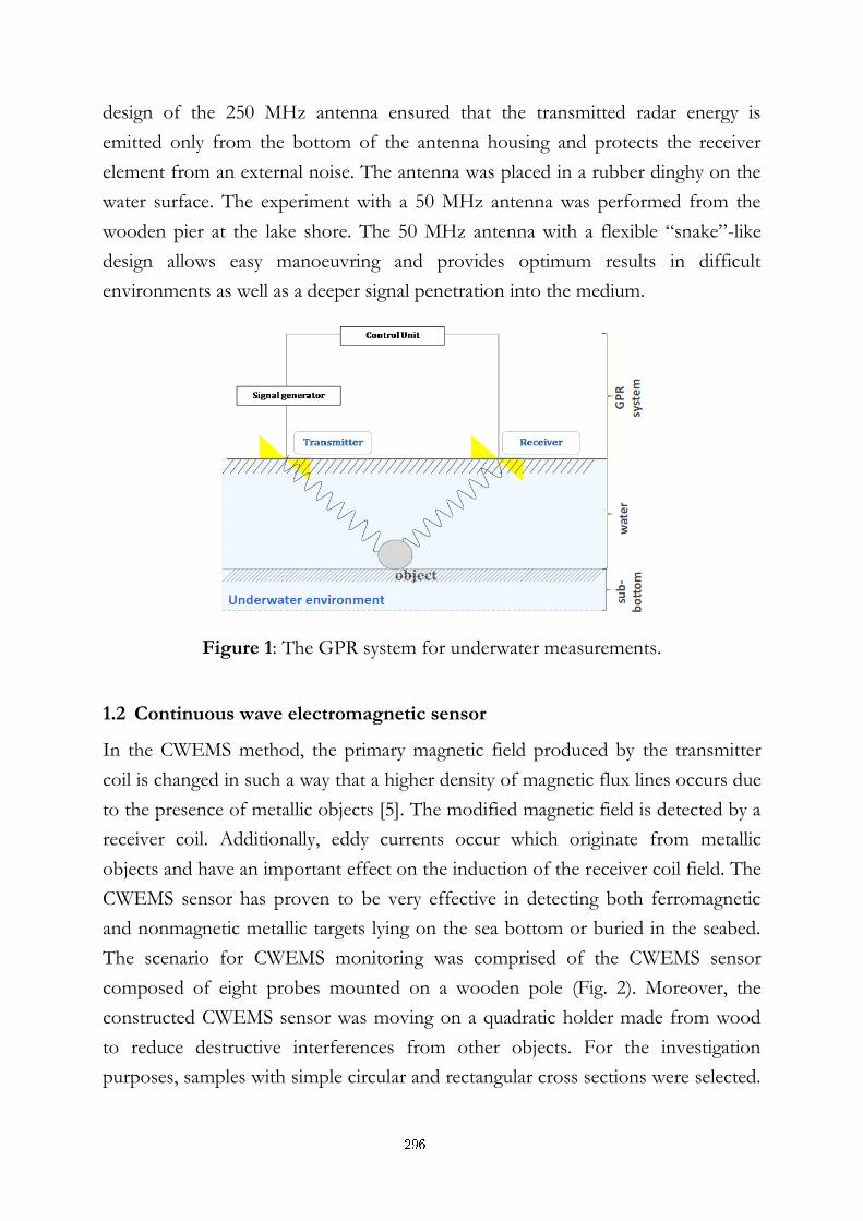
design of the 250 MHz antenna ensured that the transmitted radar energy is
emitted only from the bottom of the antenna housing and protects the receiver
element from an external noise. The antenna was placed in a rubber dinghy on the
water surface. The experiment with a 50 MHz antenna was performed from the
wooden pier at the lake shore. The 50 MHz antenna with a flexible “snake”-like
design allows easy manoeuvring and provides optimum results in difficult
environments as well as a deeper signal penetration into the medium.
Figure 1: The GPR system for underwater measurements.
1.2 Continuous wave electromagnetic sensor
In the CWEMS method, the primary magnetic field produced by the transmitter
coil is changed in such a way that a higher density of magnetic flux lines occurs due
to the presence of metallic objects [5]. The modified magnetic field is detected by a
receiver coil. Additionally, eddy currents occur which originate from metallic
objects and have an important effect on the induction of the receiver coil field. The
CWEMS sensor has proven to be very effective in detecting both ferromagnetic
and nonmagnetic metallic targets lying on the sea bottom or buried in the seabed.
The scenario for CWEMS monitoring was comprised of the CWEMS sensor
composed of eight probes mounted on a wooden pole (Fig. 2). Moreover, the
constructed CWEMS sensor was moving on a quadratic holder made from wood
to reduce destructive interferences from other objects. For the investigation
purposes, samples with simple circular and rectangular cross sections were selected.
296
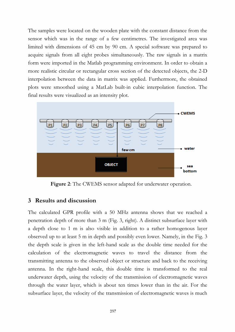
The samples were located on the wooden plate with the constant distance from the
sensor which was in the range of a few centimetres. The investigated area was
limited with dimensions of 45 cm by 90 cm. A special software was prepared to
acquire signals from all eight probes simultaneously. The raw signals in a matrix
form were imported in the Matlab programming environment. In order to obtain a
more realistic circular or rectangular cross section of the detected objects, the 2-D
interpolation between the data in matrix was applied. Furthermore, the obtained
plots were smoothed using a MatLab built-in cubic interpolation function. The
final results were visualized as an intensity plot.
Figure 2: The CWEMS sensor adapted for underwater operation.
3 Results and discussion
The calculated GPR profile with a 50 MHz antenna shows that we reached a
penetration depth of more than 3 m (Fig. 3, right). A distinct subsurface layer with
a depth close to 1 m is also visible in addition to a rather homogenous layer
observed up to at least 5 m in depth and possibly even lower. Namely, in the Fig. 3
the depth scale is given in the left-hand scale as the double time needed for the
calculation of the electromagnetic waves to travel the distance from the
transmitting antenna to the observed object or structure and back to the receiving
antenna. In the right-hand scale, this double time is transformed to the real
underwater depth, using the velocity of the transmission of electromagnetic waves
through the water layer, which is about ten times lower than in the air. For the
subsurface layer, the velocity of the transmission of electromagnetic waves is much
297
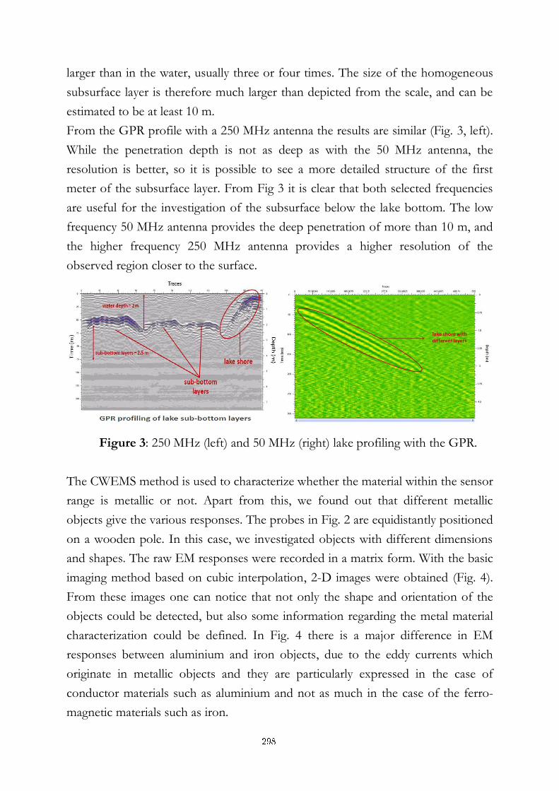
larger than in the water, usually three or four times. The size of the homogeneous
subsurface layer is therefore much larger than depicted from the scale, and can be
estimated to be at least 10 m.
From the GPR profile with a 250 MHz antenna the results are similar (Fig. 3, left).
While the penetration depth is not as deep as with the 50 MHz antenna, the
resolution is better, so it is possible to see a more detailed structure of the first
meter of the subsurface layer. From Fig 3 it is clear that both selected frequencies
are useful for the investigation of the subsurface below the lake bottom. The low
frequency 50 MHz antenna provides the deep penetration of more than 10 m, and
the higher frequency 250 MHz antenna provides a higher resolution of the
observed region closer to the surface.
Figure 3: 250 MHz (left) and 50 MHz (right) lake profiling with the GPR.
The CWEMS method is used to characterize whether the material within the sensor
range is metallic or not. Apart from this, we found out that different metallic
objects give the various responses. The probes in Fig. 2 are equidistantly positioned
on a wooden pole. In this case, we investigated objects with different dimensions
and shapes. The raw EM responses were recorded in a matrix form. With the basic
imaging method based on cubic interpolation, 2-D images were obtained (Fig. 4).
From these images one can notice that not only the shape and orientation of the
objects could be detected, but also some information regarding the metal material
characterization could be defined. In Fig. 4 there is a major difference in EM
responses between aluminium and iron objects, due to the eddy currents which
originate in metallic objects and they are particularly expressed in the case of
conductor materials such as aluminium and not as much in the case of the ferro-
magnetic materials such as iron.
298
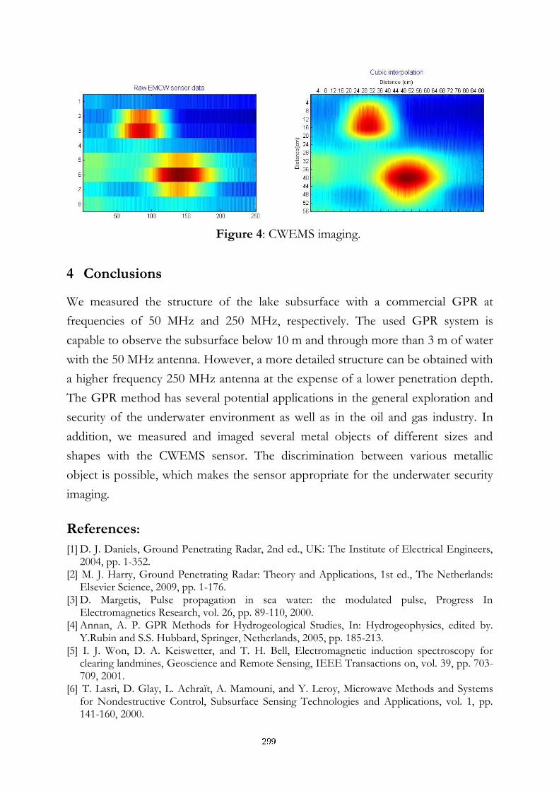
Figure 4: CWEMS imaging.
4 Conclusions
We measured the structure of the lake subsurface with a commercial GPR at
frequencies of 50 MHz and 250 MHz, respectively. The used GPR system is
capable to observe the subsurface below 10 m and through more than 3 m of water
with the 50 MHz antenna. However, a more detailed structure can be obtained with
a higher frequency 250 MHz antenna at the expense of a lower penetration depth.
The GPR method has several potential applications in the general exploration and
security of the underwater environment as well as in the oil and gas industry. In
addition, we measured and imaged several metal objects of different sizes and
shapes with the CWEMS sensor. The discrimination between various metallic
object is possible, which makes the sensor appropriate for the underwater security
imaging.
References:
[1] D. J. Daniels, Ground Penetrating Radar, 2nd ed., UK: The Institute of Electrical Engineers, 2004, pp. 1-352.
[2] M. J. Harry, Ground Penetrating Radar: Theory and Applications, 1st ed., The Netherlands: Elsevier Science, 2009, pp. 1-176.
[3] D. Margetis, Pulse propagation in sea water: the modulated pulse, Progress In Electromagnetics Research, vol. 26, pp. 89-110, 2000.
[4] Annan, A. P. GPR Methods for Hydrogeological Studies, In: Hydrogeophysics, edited by. Y.Rubin and S.S. Hubbard, Springer, Netherlands, 2005, pp. 185-213.
[5] I. J. Won, D. A. Keiswetter, and T. H. Bell, Electromagnetic induction spectroscopy for clearing landmines, Geoscience and Remote Sensing, IEEE Transactions on, vol. 39, pp. 703-709, 2001.
[6] T. Lasri, D. Glay, L. Achraït, A. Mamouni, and Y. Leroy, Microwave Methods and Systems for Nondestructive Control, Subsurface Sensing Technologies and Applications, vol. 1, pp. 141-160, 2000.
299
For wider interest
The underwater remote sensing technology plays a key role in underwater
investigation and unknown objects detection. Electromagnetic (EM) principles
have long been recognized as a useful tool for the geophysical exploration and
remote sensing. The technology that we selected includes an adapted version of the
ground penetrating radar (GPR) and the continuous wave electromagnetic sensor
(CWEMS), which are competing methods against the SONAR (sound navigation
and ranging) and metal detector. The ground penetrating radar or GPR is a non-
destructive geophysical method, which is based on the propagation of high
frequency electromagnetic waves. The GPR method images structures in the
ground that are related to changes in the dielectric properties. In addition, the
CWEMS sensor has proven to be very effective in detecting both, ferromagnetic
and nonmagnetic metallic targets, lying on the sea bottom or buried in the seabed.
We measured the structure of the lake subsurface with a commercial GPR at
frequencies of 50 MHz and 250 MHz, respectively. The used GPR system is
capable to observe the subsurface below 10 m and through more than 3 m of the
water layer with the 50 MHz antenna. However, a more detailed structure can be
obtained with a higher frequency 250 MHz antenna at the expense of a lower
penetration depth. The GPR method has several potential applications in the
general exploration and security of the underwater environment as well as in the oil
and gas industry. In addition, we measured and imaged several metal objects of
different sizes and shapes with the CWEMS sensor. The discrimination between
various metallic objects is possible, which makes the sensor appropriate for the
underwater security imaging.
300
Estimating the size of the maximum inclusion in a large sample area of steel
Nuša Pukšič1,2, Monika Jenko1
1 Institute of Metals and Technology, Ljubljana, Slovenia
2 Jožef Stefan International Postgraduate School, Ljubljana, Slovenia
Abstract. Non-metallic inclusions influence the properties of steel and
finished steel products. The methods relating to statistics of extremes are
effective for the purpose of predicting the size of the maximum inclusion,
which is an important parameter in the quality control and lifetime estimation.
A steel sample with two types of inclusions is used to demonstrate the use of
the extreme value theory in practice. The results of the general extreme value
method are compared to the results of the mixture and the competing risk
models. The competing risk model gives the best fit to data, and predicts the
largest inclusions.
Keywords: steel; inclusions; statistics of extremes; GEV; mixture; competing
risk; model
1 Introduction
Non-metallic inclusions, formed during the steel production process, have a great
impact on the properties of steel and finished steel products. The detection and
estimation of the size of the largest inclusions is an important consideration in
quality control and lifetime estimation of steel and steel products.
The size distribution of inclusions in steels is found to have a log-normal form
[1,2,3]. The standard method of fitting the log-normal distribution requires a
quantitative measurement of inclusion sizes right across the size range to obtain a
good fit. Measurements of small inclusions with sizes smaller than 3 µm are
unreliable. On the other hand, the statistic of large inclusions is affected by their
low occurrence rate.
301
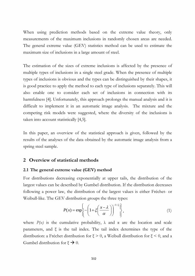
When using prediction methods based on the extreme value theory, only
measurements of the maximum inclusions in randomly chosen areas are needed.
The general extreme value (GEV) statistics method can be used to estimate the
maximum size of inclusions in a large amount of steel.
The estimation of the sizes of extreme inclusions is affected by the presence of
multiple types of inclusions in a single steel grade. When the presence of multiple
types of inclusions is obvious and the types can be distinguished by their shapes, it
is good practice to apply the method to each type of inclusions separately. This will
also enable one to consider each set of inclusions in connection with its
harmfulness [4]. Unfortunately, this approach prolongs the manual analysis and it is
difficult to implement it in an automatic image analysis. The mixture and the
competing risk models were suggested, where the diversity of the inclusions is
taken into account statistically [4,5].
In this paper, an overview of the statistical approach is given, followed by the
results of the analyses of the data obtained by the automatic image analysis from a
spring steel sample.
2 Overview of statistical methods
2.1 The general extreme value (GEV) method
For distributions decreasing exponentially at upper tails, the distribution of the
largest values can be described by Gumbel distribution. If the distribution decreases
following a power law, the distribution of the largest values is either Fréchet- or
Weibull-like. The GEV distribution groups the three types:
/1
1exp)(x
xP , (1)
where P(x) is the cumulative probability, λ and α are the location and scale
parameters, and ξ is the tail index. The tail index determines the type of the
distribution: a Fréchet distribution for ξ > 0, a Weibull distribution for ξ < 0, and a
Gumbel distribution for ξ 0.
302
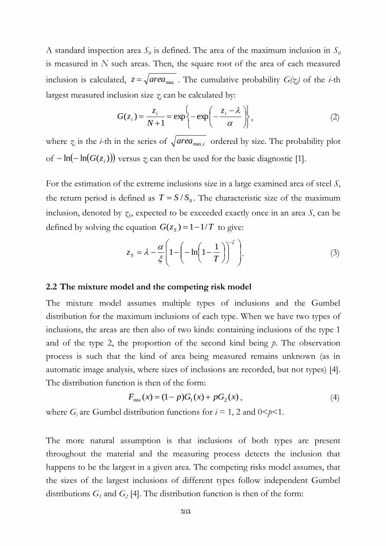
A standard inspection area S0 is defined. The area of the maximum inclusion in S0
is measured in N such areas. Then, the square root of the area of each measured
inclusion is calculated, maxareaz . The cumulative probability G(zi) of the i-th
largest measured inclusion size zi can be calculated by:
ii
i
z
N
zzG expexp
1)( , (2)
where zi is the i-th in the series of iareamax, ordered by size. The probability plot
of )(lnln izG versus zi can then be used for the basic diagnostic [1].
For the estimation of the extreme inclusions size in a large examined area of steel S,
the return period is defined as 0/ SST . The characteristic size of the maximum
inclusion, denoted by zS, expected to be exceeded exactly once in an area S, can be
defined by solving the equation TzG S /11)( to give:
TzS
11ln1 . (3)
2.2 The mixture model and the competing risk model
The mixture model assumes multiple types of inclusions and the Gumbel
distribution for the maximum inclusions of each type. When we have two types of
inclusions, the areas are then also of two kinds: containing inclusions of the type 1
and of the type 2, the proportion of the second kind being p. The observation
process is such that the kind of area being measured remains unknown (as in
automatic image analysis, where sizes of inclusions are recorded, but not types) [4].
The distribution function is then of the form:
)()()1()( 21 xpGxGpxFmix , (4)
where Gi are Gumbel distribution functions for i = 1, 2 and 0<p<1.
The more natural assumption is that inclusions of both types are present
throughout the material and the measuring process detects the inclusion that
happens to be the largest in a given area. The competing risks model assumes, that
the sizes of the largest inclusions of different types follow independent Gumbel
distributions G1 and G2 [4]. The distribution function is then of the form:
303
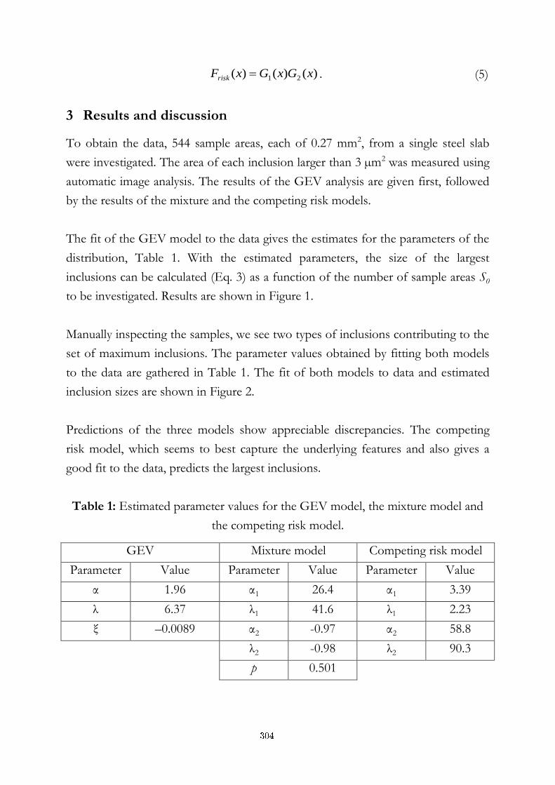
)()()( 21 xGxGxFrisk . (5)
3 Results and discussion
To obtain the data, 544 sample areas, each of 0.27 mm2, from a single steel slab
were investigated. The area of each inclusion larger than 3 µm2 was measured using
automatic image analysis. The results of the GEV analysis are given first, followed
by the results of the mixture and the competing risk models.
The fit of the GEV model to the data gives the estimates for the parameters of the
distribution, Table 1. With the estimated parameters, the size of the largest
inclusions can be calculated (Eq. 3) as a function of the number of sample areas S0
to be investigated. Results are shown in Figure 1.
Manually inspecting the samples, we see two types of inclusions contributing to the
set of maximum inclusions. The parameter values obtained by fitting both models
to the data are gathered in Table 1. The fit of both models to data and estimated
inclusion sizes are shown in Figure 2.
Predictions of the three models show appreciable discrepancies. The competing
risk model, which seems to best capture the underlying features and also gives a
good fit to the data, predicts the largest inclusions.
Table 1: Estimated parameter values for the GEV model, the mixture model and
the competing risk model.
GEV Mixture model Competing risk model
Parameter Value Parameter Value Parameter Value
α 1.96 α1 26.4 α1 3.39
λ 6.37 λ1 41.6 λ1 2.23
ξ –0.0089 α2 -0.97 α2 58.8
λ2 -0.98 λ2 90.3
p 0.501
304
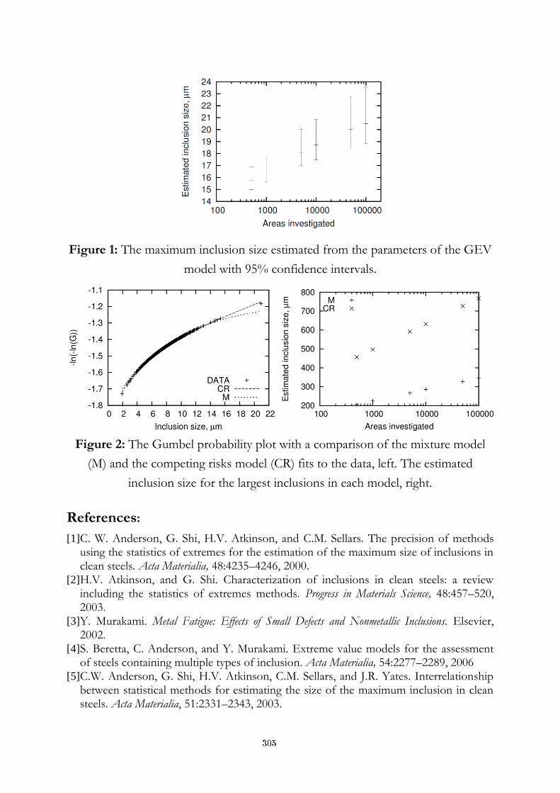
Figure 1: The maximum inclusion size estimated from the parameters of the GEV
model with 95% confidence intervals.
Figure 2: The Gumbel probability plot with a comparison of the mixture model
(M) and the competing risks model (CR) fits to the data, left. The estimated
inclusion size for the largest inclusions in each model, right.
References:
[1] C. W. Anderson, G. Shi, H.V. Atkinson, and C.M. Sellars. The precision of methods using the statistics of extremes for the estimation of the maximum size of inclusions in clean steels. Acta Materialia, 48:4235–4246, 2000.
[2] H.V. Atkinson, and G. Shi. Characterization of inclusions in clean steels: a review including the statistics of extremes methods. Progress in Materials Science, 48:457–520, 2003.
[3] Y. Murakami. Metal Fatigue: Effects of Small Defects and Nonmetallic Inclusions. Elsevier, 2002.
[4] S. Beretta, C. Anderson, and Y. Murakami. Extreme value models for the assessment of steels containing multiple types of inclusion. Acta Materialia, 54:2277–2289, 2006
[5] C.W. Anderson, G. Shi, H.V. Atkinson, C.M. Sellars, and J.R. Yates. Interrelationship between statistical methods for estimating the size of the maximum inclusion in clean steels. Acta Materialia, 51:2331–2343, 2003.
305

For wider interest
The properties of steel and finished steel products are affected by non-metallic
inclusions, formed during the steel production process. The detection and
estimation of the size of the largest inclusions can be an important parameter in the
quality control and lifetime estimation of steel and steel products. Statistical
methods can be helpful, since they can provide an additional insight not necessarily
apparent from the raw data. There are a few options that allow us to estimate the
size of the largest inclusion to be expected. Unfortunately, there can be great
discrepancies in the predictions from different models. Care should be taken when
choosing a method and a model to investigate and analyse your product. Any of the
models presented in this paper, on the other hand, can be used as a means of
comparing different grades of steels or to define bounds, within which the quality
of a given grade of steel is still acceptable.
306
Solvent capabilities of liquid and supercritical xenon
Kristian Radan, Boris Žemva
Department of Inorganic Chemistry and Technology, Jamova 39, Jožef Stefan
Institute, Ljubljana, Slovenia
Jožef Stefan International Postgraduate School, Ljubljana, Slovenia
Abstract. A great majority of “interesting” compounds in fluorine and noble
gas chemistry are thermodynamically unstable, highly oxidative and thus hard
to isolate and characterize materials. Since the ultimate characterization -
structural determination is very often related to a route to crystalline products,
the aforementioned unique properties severely restrict the choice of a solvent
for these compounds to a few inorganic (BrF5, IF5, SF6, anhydrous HF,
SOClF, etc.) and in some cases organic solvents (CH3CN,
fluorotrichloromethane, etc.). However, several coordination complexes with
noble gas fluorides for example, especially those with large polyionic units [1],
remain insoluble in solvents mentioned above. In this work we report some
preliminary results of three experiments made in order to investigate the
solvent potential of liquid and near-supercritical xenon on these systems.
Keywords: inorganic fluorides, compounds of noble gases, liquid xenon,
supercritical xenon.
1 Introduction
The idea of using liquid xenon as a solvent is not new. The experimental evidence
was presented by Rentzepis and Douglass in 1981 in the form of UV, visible, IR
and NMR spectra which showed that liquid Xe can be used as a fluid solvent for
several biological and organic molecules at temperatures ranging from near room
temperature to about –100 °C [2].
Xenon is particularly useful among the noble gases because its liquid phase occurs
in the fairly convenient conditions of ~16 °C and 58 atm, so that solution studies
can be carried out near room temperature (Fig. 1). Xenon also possesses a
307
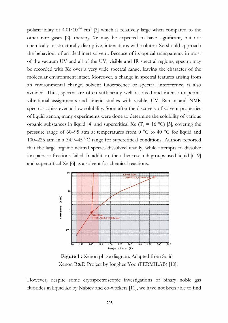
polarizability of 4.01·10-24 cm3 [3] which is relatively large when compared to the
other rare gases [2], thereby Xe may be expected to have significant, but not
chemically or structurally disruptive, interactions with solutes: Xe should approach
the behaviour of an ideal inert solvent. Because of its optical transparency in most
of the vacuum UV and all of the UV, visible and IR spectral regions, spectra may
be recorded with Xe over a very wide spectral range, leaving the character of the
molecular environment intact. Moreover, a change in spectral features arising from
an environmental change, solvent fluorescence or spectral interference, is also
avoided. Thus, spectra are often sufficiently well resolved and intense to permit
vibrational assignments and kinetic studies with visible, UV, Raman and NMR
spectroscopies even at low solubility. Soon after the discovery of solvent properties
of liquid xenon, many experiments were done to determine the solubility of various
organic substances in liquid [4] and supercritical Xe (Tc = 16 °C) [5], covering the
pressure range of 60–95 atm at temperatures from 0 °C to 40 °C for liquid and
100–225 atm in a 34.9–45 °C range for supercritical conditions. Authors reported
that the large organic neutral species dissolved readily, while attempts to dissolve
ion pairs or free ions failed. In addition, the other research groups used liquid [6–9]
and supercritical Xe [6] as a solvent for chemical reactions.
Figure 1 : Xenon phase diagram. Adapted from Solid
Xenon R&D Project by Jonghee Yoo (FERMILAB) [10].
However, despite some cryospectroscopic investigations of binary noble gas
fluorides in liquid Xe by Nabiev and co-workers [11], we have not been able to find
308
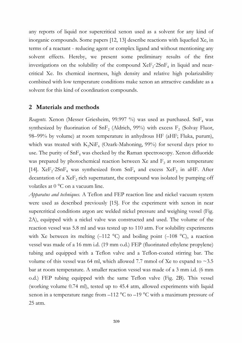
any reports of liquid nor supercritical xenon used as a solvent for any kind of
inorganic compounds. Some papers [12, 13] describe reactions with liquefied Xe, in
terms of a reactant - reducing agent or complex ligand and without mentioning any
solvent effects. Hereby, we present some preliminary results of the first
investigations on the solubility of the compound XeF2·2SnF4 in liquid and near-
critical Xe. Its chemical inertness, high density and relative high polarizability
combined with low temperature conditions make xenon an attractive candidate as a
solvent for this kind of coordination compounds.
2 Materials and methods
Reagents. Xenon (Messer Griesheim, 99.997 %) was used as purchased. SnF4 was
synthesized by fluorination of SnF2 (Aldrich, 99%) with excess F2 (Solvay Fluor,
98–99% by volume) at room temperature in anhydrous HF (aHF; Fluka, purum),
which was treated with K2NiF6 (Ozark-Mahoning, 99%) for several days prior to
use. The purity of SnF4 was checked by the Raman spectroscopy. Xenon difluoride
was prepared by photochemical reaction between Xe and F2 at room temperature
[14]. XeF2·2SnF4 was synthesized from SnF4 and excess XeF2 in aHF. After
decantation of a XeF2 rich supernatant, the compound was isolated by pumping off
volatiles at 0 °C on a vacuum line.
Apparatus and techniques. A Teflon and FEP reaction line and nickel vacuum system
were used as described previously [15]. For the experiment with xenon in near
supercritical conditions argon arc welded nickel pressure and weighing vessel (Fig.
2A), equipped with a nickel valve was constructed and used. The volume of the
reaction vessel was 5.8 ml and was tested up to 110 atm. For solubility experiments
with Xe between its melting (–112 °C) and boiling point (–108 °C), a reaction
vessel was made of a 16 mm i.d. (19 mm o.d.) FEP (fluorinated ethylene propylene)
tubing and equipped with a Teflon valve and a Teflon-coated stirring bar. The
volume of this vessel was 64 ml, which allowed 7.7 mmol of Xe to expand to ~3.5
bar at room temperature. A smaller reaction vessel was made of a 3 mm i.d. (6 mm
o.d.) FEP tubing equipped with the same Teflon valve (Fig. 2B). This vessel
(working volume 0.74 ml), tested up to 45.4 atm, allowed experiments with liquid
xenon in a temperature range from –112 °C to –19 °C with a maximum pressure of
25 atm.
309
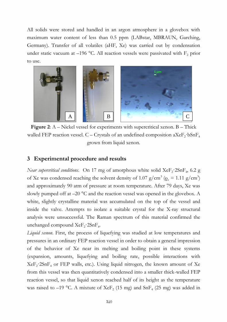
All solids were stored and handled in an argon atmosphere in a glovebox with
maximum water content of less than 0.5 ppm (LABstar, MBRAUN, Garching,
Germany). Transfer of all volatiles (aHF, Xe) was carried out by condensation
under static vacuum at –196 °C. All reaction vessels were passivated with F2 prior
to use.
Figure 2: A – Nickel vessel for experiments with supercritical xenon. B – Thick
walled FEP reaction vessel. C – Crystals of an undefined composition aXeF2·bSnF4
grown from liquid xenon.
3 Experimental procedure and results
Near supercritical conditions. On 17 mg of amorphous white solid XeF2·2SnF4, 6.2 g
of Xe was condensed reaching the solvent density of 1.07 g/cm3 (ρc = 1.11 g/cm3)
and approximately 90 atm of pressure at room temperature. After 79 days, Xe was
slowly pumped off at –20 °C and the reaction vessel was opened in the glovebox. A
white, slightly crystalline material was accumulated on the top of the vessel and
inside the valve. Attempts to isolate a suitable crystal for the X-ray structural
analysis were unsuccessful. The Raman spectrum of this material confirmed the
unchanged compound XeF2·2SnF4.
Liquid xenon. First, the process of liquefying was studied at low temperatures and
pressures in an ordinary FEP reaction vessel in order to obtain a general impression
of the behavior of Xe near its melting and boiling point in these systems
(expansion, amounts, liquefying and boiling rate, possible interactions with
XeF2·2SnF4 or FEP walls, etc.). Using liquid nitrogen, the known amount of Xe
from this vessel was then quantitatively condensed into a smaller thick-walled FEP
reaction vessel, so that liquid xenon reached half of its height as the temperature
was raised to –19 °C. A mixture of XeF2 (15 mg) and SnF4 (25 mg) was added in
A B C
310
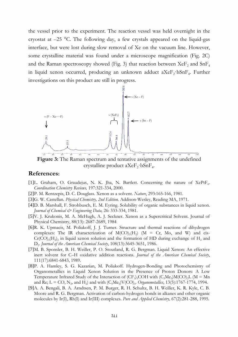
the vessel prior to the experiment. The reaction vessel was held overnight in the
cryostat at –25 °C. The following day, a few crystals appeared on the liquid-gas
interface, but were lost during slow removal of Xe on the vacuum line. However,
some crystalline material was found under a microscope magnification (Fig. 2C)
and the Raman spectroscopy showed (Fig. 3) that reaction between XeF2 and SnF4
in liquid xenon occurred, producing an unknown adduct aXeF2·bSnF4. Further
investigations on this product are still in progress.
Figure 3: The Raman spectrum and tentative assignments of the undefined crystalline product aXeF2·bSnF4.
References:
[1] L. Graham, O. Graudejus, N. K. Jha, N. Bartlett. Concerning the nature of XePtF6. Coordination Chemistry Reviews, 197:321-334, 2000.
[2] P. M. Rentzepis, D. C. Douglass. Xenon as a solvent. Nature, 293:165-166, 1981.
[3] G. W. Castellan. Physical Chemistry, 2nd Edition. Addison-Wesley, Reading MA, 1971.
[4] D. B. Marshall, F. Strohbusch, E. M. Eyring. Solubility of organic substances in liquid xenon. Journal of Chemical & Engineering Data, 26: 333-334, 1981.
[5] V. J. Krukonis, M. A. McHugh, A. J. Seckner. Xenon as a Supercritical Solvent. Journal of Physical Chemistry, 88(13): 2687-2689, 1984
[6] R. K. Upmacis, M. Poliakoff, J. J. Turner. Structure and thermal reactions of dihydrogen complexes: The IR characterization of M(CO)5(H2) (M = Cr, Mo, and W) and cis-Cr(CO)4(H2)2 in liquid xenon solution and the formation of HD during exchange of H2 and D2. Journal of the American Chemical Society, 108(13):3645-3651, 1986.
[7] M. B. Sponsler, B. H. Weiller, P. O. Stoutland, R. G. Bergman. Liquid Xenon: An effective inert solvent for C–H oxidative addition reactions. Journal of the American Chemical Society, 111(17):6841-6843, 1989.
[8] P. A. Hamley, S. G. Kazarian, M. Poliakoff. Hydrogen-Bonding and Photochemistry of Organometallics in Liquid Xenon Solution in the Presence of Proton Donors: A Low Temperature Infrared Study of the Interaction of (CF3)3COH with (C5Me5)M(CO)2L (M = Mn and Re; L = CO, N2, and H2) and with (C5Me5)V(CO)4. Organometallics, 13(5):1767-1774, 1994.
[9] A. A. Bengali, B. A. Arndtsen, P. M. Burger, R. H. Schultz, B. H. Weiller, K. R. Kyle, C. B. Moore and R. G. Bergman. Activation of carbon-hydrogen bonds in alkanes and other organic molecules by Ir(I), Rh(I) and Ir(III) complexes. Pure and Applied Chemistry, 67(2):281-288, 1995.
ν (F – Xe····F) ν (XeF2)
ν (Xe – F)
ν (Sn – F)
311

[10] Jonghee Yoo. Solid Xenon project at Fermilab. In Dark Matter 2010 Presentations, Ninth UCLA Symposium on Sources and Detection of Dark Matter and Dark Energy in the Universe, Marina del Rey, California, USA, 2010.
[11] Sh.Sh. Nablev, V.D. Klimov, B.S. Khodiev. Cryospectroscopic analysis of individual xenon fluorides. Journal of Fluorine Chemistry, 58(2-3):293, 1992.
[12] C. T. Goetschel, K. R. Loos. Reaction of xenon with dioxygenyl tetrafluoroborate. Preparation of FXe-BF2. Journal of the American Chemical Society, 94(9):3018-3021, 1972.
[13] S. Seidel, K. Seppelt, C. van Wüllen, X. Y. Sun. The Blue Xe4+ Cation: Experimental
Detection and Theoretical Characterization. Angewandte Chemie International Edition, 46(35):6717-6720, 2007.
[14] A. Šmalc, K. Lutar. Inorganic Syntheses, Vol. 29. R. N. Grimes, 1992.
[15] H. Borrmann, K. Lutar, B. Žemva. Manganese(II) Hexafluoroarsenate: Unusually High Coordination of Manganese(II) in a Fluorine Environment. Inorganic Chemistry, 36(5):880–882, 1997.
312
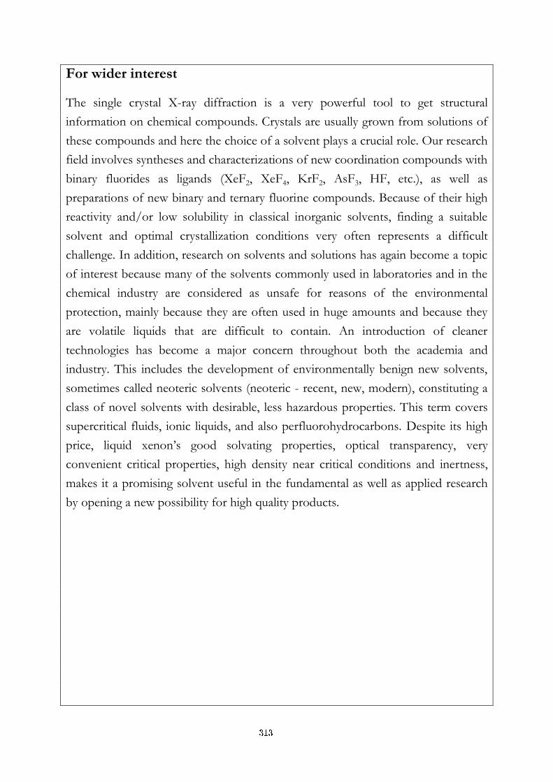
For wider interest
The single crystal X-ray diffraction is a very powerful tool to get structural
information on chemical compounds. Crystals are usually grown from solutions of
these compounds and here the choice of a solvent plays a crucial role. Our research
field involves syntheses and characterizations of new coordination compounds with
binary fluorides as ligands (XeF2, XeF4, KrF2, AsF3, HF, etc.), as well as
preparations of new binary and ternary fluorine compounds. Because of their high
reactivity and/or low solubility in classical inorganic solvents, finding a suitable
solvent and optimal crystallization conditions very often represents a difficult
challenge. In addition, research on solvents and solutions has again become a topic
of interest because many of the solvents commonly used in laboratories and in the
chemical industry are considered as unsafe for reasons of the environmental
protection, mainly because they are often used in huge amounts and because they
are volatile liquids that are difficult to contain. An introduction of cleaner
technologies has become a major concern throughout both the academia and
industry. This includes the development of environmentally benign new solvents,
sometimes called neoteric solvents (neoteric - recent, new, modern), constituting a
class of novel solvents with desirable, less hazardous properties. This term covers
supercritical fluids, ionic liquids, and also perfluorohydrocarbons. Despite its high
price, liquid xenon’s good solvating properties, optical transparency, very
convenient critical properties, high density near critical conditions and inertness,
makes it a promising solvent useful in the fundamental as well as applied research
by opening a new possibility for high quality products.
313
A chemometric approach towards transmembrane region prediction of protein sequences
Amrita Roy Choudhury1,2, Marjana Novič1
1 Laboratory of Chemometrics, National Institute of Chemistry, Ljubljana, Slovenia
2 Jožef Stefan International Postgraduate School, Ljubljana, Slovenia
Abstract. Transmembrane proteins play vital roles in maintaining the normal
cell physiology. They are also important as potential drug targets. Therefore,
there is an immense academic and pharmaceutical interest in these proteins. In
our lab, we have tried to use chemometric approach along with other
computational and experimental methods towards elucidation of
transmembrane protein structures and functional mechanisms. Here we
present a data-driven chemometric classification model based on mathematical
descriptors to discriminate between transmembrane and non-transmembrane
regions of protein sequences. The model is then utilized to predict the
transmembrane regions of specific proteins, and also to differentiate between
transmembrane and globular proteins.
Keywords: chemometric model, transmembrane region prediction tool, amino
acid adjacency matrix, mathematical descriptors.
1 Introduction
Transmembrane proteins play crucial roles acting as transporters, receptors, helping
in cell signalling etc., and thus help to maintain the normal cell functioning. They
are also of interest for the pharmaceutical industry with more than a half of the
drugs currently available on the market targeting the transmembrane proteins [1].
However, the structures and functional mechanisms of a very few of these proteins
are known down to date owing to experimental difficulties. Although, around 25%
of the Open Reading Frames code for transmembrane proteins, they account for
only ~2% of the Protein Data Bank (PDB) structures [2]. A vast majority of these
proteins, therefore, remain unexplored and present challenges to both
computational and experimental procedures. Our aim is to utilize different
314
chemometric approaches in coordination with experimental and other
computational methods towards working in this direction.
The first step towards the elucidation of structures and functional mechanisms of
transmembrane proteins is to know the exact number and position of their
transmembrane regions. For this purpose, we have developed a transmembrane
region prediction algorithm, based on mathematical descriptors and neural
networks. The advantage of our algorithm over other existing ones is that it uses
mathematical descriptors derived from the sequence information alone, and is
independent of physiochemical property indices and evolutionary information. The
algorithm is able to well discriminate between the transmembrane and the non-
transmembrane regions of the α-transmembrane proteins. The developed model is
then used to predict the transmembrane regions of unknown protein sequences [3].
2 Methodology
2.1 Dataset used
We collect α-transmembrane protein sequences and information from databases
PDB and Protein Data Bank of Transmembrane Proteins (PDBTM) [2], [4]. The
sequences are checked for redundancy and low-resolution data. Each sequence is
then segmented into its transmembrane and non-transmembrane regions. The final
dataset contains 552 protein chains, divided into 2545 transmembrane and 3255
non-transmembrane segments.
2.2 Amino acid adjacency matrix
In building the chemometric classification model, we have used mathematical
descriptors derived from amino acid adjacency matrices to characterize the protein
segments. The amino acid adjacency matrix is a 20×20 matrix with the rows and
columns labelled with the 20 amino acids [5]. Each position in the matrix denotes
the number of times the corresponding amino acids occur as neighbours in the
sequence (Fig. 1). The 20-element rowsum vector of the amino acid adjacency
matrix is used as the descriptor set to represent the protein segments in our model.
All the transmembrane and non-transmembrane regions of the protein sequences
are encoded accordingly into the mathematical descriptors. The advantage of the
descriptors is that they are dependent only on the sequence information.
315

Figure 1: The amino acid adjacency matrix and 20-element rowsum vector of the
given protein sequence.
2.3 Classification model
The mathematically encoded transmembrane and non-transmembrane segments
are divided into training, test and external validation sets using the Kohonnen
network. We use the non-linear modelling method the Counter Propagation Neural
network (CPNN) to build the classification model [6]. The model is trained and
optimized using the training and test sets with varying network parameters. The
optimized network, i.e., the one with a minimum error in recall and prediction
abilities, is then challenged with the external validation set that is not used in any of
the previous model optimization steps.
2.4 Transmembrane region prediction tool
The developed classification model is used for the transmembrane region
prediction of unknown protein sequences [3]. For this purpose, a sliding window
approach is used with the window size of 20 residues for the α-transmembrane
proteins. Each window segment is then fed into the classification model for its
prediction as transmembrane or non-transmembrane. As the segments are
overlapping, the central residues covered by 10 or more consecutive overlapping
316
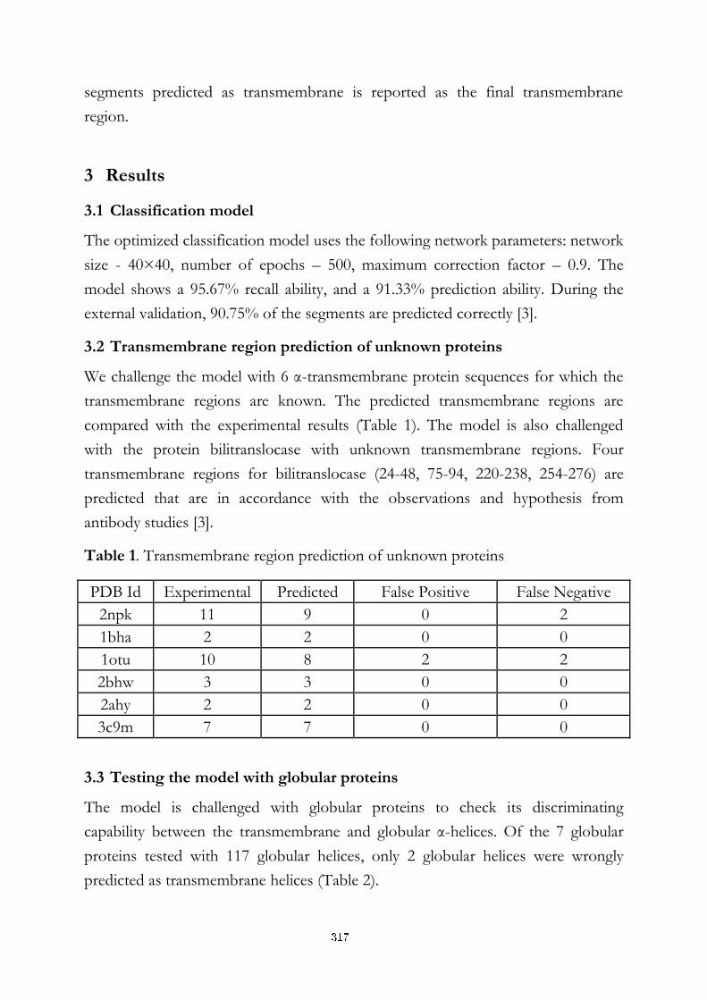
segments predicted as transmembrane is reported as the final transmembrane
region.
3 Results
3.1 Classification model
The optimized classification model uses the following network parameters: network
size - 40×40, number of epochs – 500, maximum correction factor – 0.9. The
model shows a 95.67% recall ability, and a 91.33% prediction ability. During the
external validation, 90.75% of the segments are predicted correctly [3].
3.2 Transmembrane region prediction of unknown proteins
We challenge the model with 6 α-transmembrane protein sequences for which the
transmembrane regions are known. The predicted transmembrane regions are
compared with the experimental results (Table 1). The model is also challenged
with the protein bilitranslocase with unknown transmembrane regions. Four
transmembrane regions for bilitranslocase (24-48, 75-94, 220-238, 254-276) are
predicted that are in accordance with the observations and hypothesis from
antibody studies [3].
Table 1. Transmembrane region prediction of unknown proteins
PDB Id Experimental Predicted False Positive False Negative
2npk 11 9 0 2
1bha 2 2 0 0
1otu 10 8 2 2
2bhw 3 3 0 0
2ahy 2 2 0 0
3c9m 7 7 0 0
3.3 Testing the model with globular proteins
The model is challenged with globular proteins to check its discriminating
capability between the transmembrane and globular α-helices. Of the 7 globular
proteins tested with 117 globular helices, only 2 globular helices were wrongly
predicted as transmembrane helices (Table 2).
317
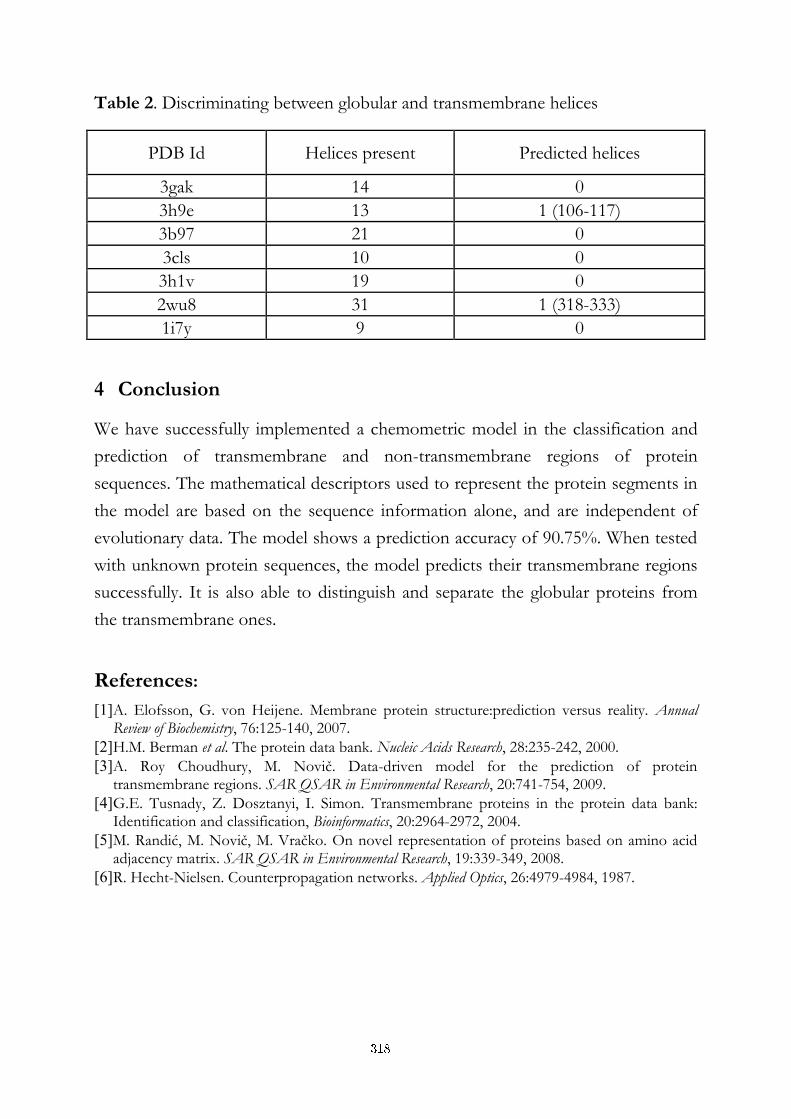
Table 2. Discriminating between globular and transmembrane helices
PDB Id Helices present Predicted helices
3gak 14 0
3h9e 13 1 (106-117)
3b97 21 0
3cls 10 0
3h1v 19 0
2wu8 31 1 (318-333)
1i7y 9 0
4 Conclusion
We have successfully implemented a chemometric model in the classification and
prediction of transmembrane and non-transmembrane regions of protein
sequences. The mathematical descriptors used to represent the protein segments in
the model are based on the sequence information alone, and are independent of
evolutionary data. The model shows a prediction accuracy of 90.75%. When tested
with unknown protein sequences, the model predicts their transmembrane regions
successfully. It is also able to distinguish and separate the globular proteins from
the transmembrane ones.
References:
[1] A. Elofsson, G. von Heijene. Membrane protein structure:prediction versus reality. Annual Review of Biochemistry, 76:125-140, 2007.
[2] H.M. Berman et al. The protein data bank. Nucleic Acids Research, 28:235-242, 2000.
[3] A. Roy Choudhury, M. Novič. Data-driven model for the prediction of protein transmembrane regions. SAR QSAR in Environmental Research, 20:741-754, 2009.
[4] G.E. Tusnady, Z. Dosztanyi, I. Simon. Transmembrane proteins in the protein data bank: Identification and classification, Bioinformatics, 20:2964-2972, 2004.
[5] M. Randić, M. Novič, M. Vračko. On novel representation of proteins based on amino acid adjacency matrix. SAR QSAR in Environmental Research, 19:339-349, 2008.
[6] R. Hecht-Nielsen. Counterpropagation networks. Applied Optics, 26:4979-4984, 1987.
318
For wider interest
Transmembrane proteins are membrane proteins spanning the whole biological
membrane, acting both as barriers and communication channels between the
intracellular and the extracellular spaces. They play crucial roles in the cell
functioning acting as the transporters and receptors of various ligands, helping in
the cell signalling etc. In addition, they are important as drug targets. However, the
transmembrane proteins remain vastly unexplored due to experimental difficulties.
Most of these proteins have unknown structures, and those with known structures
often remain poorly annotated. Several interdisciplinary computational approaches
along with experimental ones are therefore used to gain insights into the
transmembrane proteins. Our lab expertizes: (i) the development and applications
of standard and modern chemometrics techniques (clustering, classification,
modelling, neural networks, genetic algorithms); (ii) handling of large amounts of
multivariate data: transformations, projections, reductions, selection of variables
and optimization of the data-representation for different modelling approaches; (iii)
modelling using linear or non-linear methods – case studies in (Quantitative
Structure-Activity Relationship) QSAR (modelling of biological properties), in
analytical chemistry, determination of 3D molecular structures, calculation of
descriptors and structure representations; validation of QSAR models. Our aim is
to utilize this expertise for the characterization of transmembrane proteins using
different chemometric methods for their structural elucidation. In the first step
reported here, we have successfully developed a novel transmembrane region
prediction algorithm. It is based on mathematical descriptors and neural networks.
The prediction method, based on the sequence information, is independent of
evolutionary data and physiochemical properties. The model is able to both predict
successfully the transmembrane regions of unknown protein sequences and
distinguish them from globular proteins. In the future, our aim is to utilize the data
obtained from the inhibition studies applying chemometric tools, along with other
computational and experimental methods, to study and predict the transport
function of specific transmembrane proteins; and we are currently already working
on these items. The chemometric methods along with other computational and
experimental procedures, can be a very powerful aid to elucidate the structures and
functional mechanisms of various transmembrane proteins.
319
Vpliv legirnih elementov na lomno žilavost vzmetnega jekla
51CrV4
Bojan Senčič1,2
Vojteh Leskovšek3
1 ŠTORE STEEL d.o.o., Železarska cesta 3, Štore, Slovenija
2 Mednarodna podiplomska šola Jožefa Stefana, Jamova 39, Ljubljana, Slovenija
3 Inštitut za kovinske materiale in tehnologije, Lepi pot 11, Ljubljana, Slovenija
Povzetek. Za izdelavo listnatih vzmeti se večinoma uporablja vzmetno jeklo
51CrV4. Ker je v avtomobilski industriji prisoten stalen trend po zmanjševanju
mase komponent, potrebujejo proizvajalci vzmeti jekla z izrednimi
mehanskimi lastnostmi, med katerimi je zaradi želene visoke trajne dinamične
trdnosti še posebej pomembna lomna žilavost KIc. Izdelano je bilo več jekel z
različnimi dodatki Nb, Mo, C, Al in Ca. Z nestandardnim postopkom
preizkušanja lomne žilavosti s cilindričnim nateznim preizkušancem z zarezo
po obodu in utrujenostno razpoko v dnu zareze smo raziskali vpliv legirnih
elementov na lomno žilavost pri enaki trdoti Rockwell-C vakuumsko toplotno
obdelanega vzmetnega jekla.
Ugotovili smo, da določen dodatek legiranih elementov pozitivno vpliva na
lomno žilavost KIc.
Ključne besede: lomna žilavost, vzmetno jeklo, legirni elementi, diagram
popuščanja.
1 Uvod
V avtomobilski industriji se za izdelavo listnatih vzmeti uporablja predvsem
vzmetno jeklo 51CrV4. Zaradi stalnega trenda po zmanjševanju mase vozil tudi
proizvajalci vzmeti težijo k zmanjševanju mase vzmeti. Zato potrebujejo jekla z
boljšimi mehanskimi lastnostmi, med katerimi pa je še posebej pomembna lomna
žilavost KIc. Namen raziskovalne naloge je bil, da raziščemo vpliv dodatka različnih
legirnih elementov na lomno žilavost, ki smo jo merili z nestandardnim postopkom
320
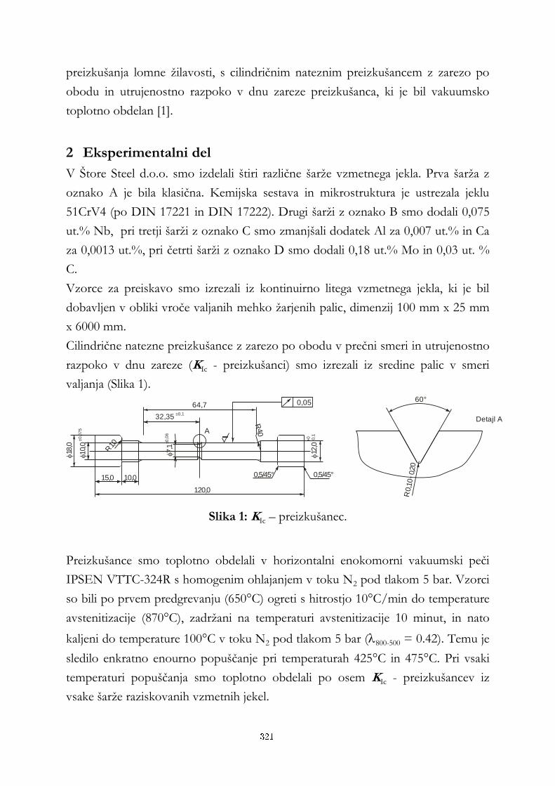
preizkušanja lomne žilavosti, s cilindričnim nateznim preizkušancem z zarezo po
obodu in utrujenostno razpoko v dnu zareze preizkušanca, ki je bil vakuumsko
toplotno obdelan [1].
2 Eksperimentalni del
V Štore Steel d.o.o. smo izdelali štiri različne šarže vzmetnega jekla. Prva šarža z
oznako A je bila klasična. Kemijska sestava in mikrostruktura je ustrezala jeklu
51CrV4 (po DIN 17221 in DIN 17222). Drugi šarži z oznako B smo dodali 0,075
ut.% Nb, pri tretji šarži z oznako C smo zmanjšali dodatek Al za 0,007 ut.% in Ca
za 0,0013 ut.%, pri četrti šarži z oznako D smo dodali 0,18 ut.% Mo in 0,03 ut. %
C.
Vzorce za preiskavo smo izrezali iz kontinuirno litega vzmetnega jekla, ki je bil
dobavljen v obliki vroče valjanih mehko žarjenih palic, dimenzij 100 mm x 25 mm
x 6000 mm.
Cilindrične natezne preizkušance z zarezo po obodu v prečni smeri in utrujenostno
razpoko v dnu zareze (KIc - preizkušanci) smo izrezali iz sredine palic v smeri
valjanja (Slika 1).
Detajl A
A
60°R
0,1
0 - 0,
20
R 1,0
f18
,0
f10,
0
f7,1
f12
,0
R 4,0
15,0 10,0
120,0
64,7
±0
,07
5
+0
-0,1
±0,0
6
0,5/45° 0,5/45°
32,35±0,1
0,05
Slika 1: KIc – preizkušanec.
Preizkušance smo toplotno obdelali v horizontalni enokomorni vakuumski peči
IPSEN VTTC-324R s homogenim ohlajanjem v toku N2 pod tlakom 5 bar. Vzorci
so bili po prvem predgrevanju (650°C) ogreti s hitrostjo 10°C/min do temperature
avstenitizacije (870°C), zadržani na temperaturi avstenitizacije 10 minut, in nato
kaljeni do temperature 100°C v toku N2 pod tlakom 5 bar (800-500 = 0.42). Temu je
sledilo enkratno enourno popuščanje pri temperaturah 425°C in 475°C. Pri vsaki
temperaturi popuščanja smo toplotno obdelali po osem KIc - preizkušancev iz
vsake šarže raziskovanih vzmetnih jekel.
321
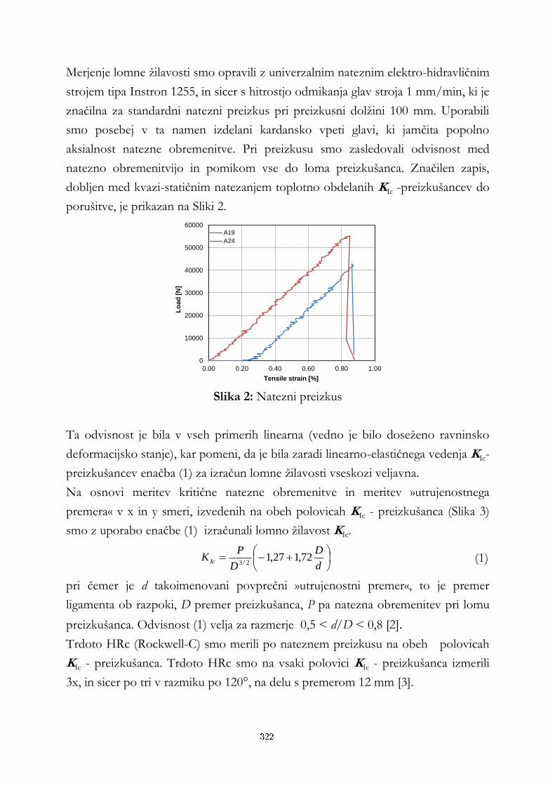
Merjenje lomne žilavosti smo opravili z univerzalnim nateznim elektro-hidravličnim
strojem tipa Instron 1255, in sicer s hitrostjo odmikanja glav stroja 1 mm/min, ki je
značilna za standardni natezni preizkus pri preizkusni dolžini 100 mm. Uporabili
smo posebej v ta namen izdelani kardansko vpeti glavi, ki jamčita popolno
aksialnost natezne obremenitve. Pri preizkusu smo zasledovali odvisnost med
natezno obremenitvijo in pomikom vse do loma preizkušanca. Značilen zapis,
dobljen med kvazi-statičnim natezanjem toplotno obdelanih KIc -preizkušancev do
porušitve, je prikazan na Sliki 2.
0
10000
20000
30000
40000
50000
60000
0.00 0.20 0.40 0.60 0.80 1.00
Lo
ad
[N
]
Tensile strain [%]
A19
A24
Slika 2: Natezni preizkus
Ta odvisnost je bila v vseh primerih linearna (vedno je bilo doseženo ravninsko
deformacijsko stanje), kar pomeni, da je bila zaradi linearno-elastičnega vedenja KIc-
preizkušancev enačba (1) za izračun lomne žilavosti vseskozi veljavna.
Na osnovi meritev kritične natezne obremenitve in meritev »utrujenostnega
premera« v x in y smeri, izvedenih na obeh polovicah KIc - preizkušanca (Slika 3)
smo z uporabo enačbe (1) izračunali lomno žilavost KIc.
d
D
D
PK Ic 72,127,1
2/3 (1)
pri čemer je d takoimenovani povprečni »utrujenostni premer«, to je premer
ligamenta ob razpoki, D premer preizkušanca, P pa natezna obremenitev pri lomu
preizkušanca. Odvisnost (1) velja za razmerje 0,5 < d/D < 0,8 [2].
Trdoto HRc (Rockwell-C) smo merili po nateznem preizkusu na obeh polovicah
KIc - preizkušanca. Trdoto HRc smo na vsaki polovici KIc - preizkušanca izmerili
3x, in sicer po tri v razmiku po 120°, na delu s premerom 12 mm [3].
322
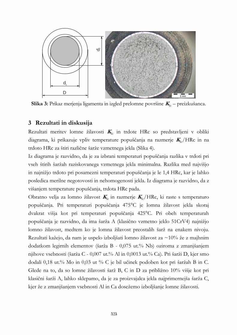
d1
d2
D
Slika 3: Prikaz merjenja ligamenta in izgled prelomne površine KIc – preizkušanca.
3 Rezultati in diskusija
Rezultati meritev lomne žilavosti KIc in trdote HRc so predstavljeni v obliki
diagrama, ki prikazuje vpliv temperature popuščanja na razmerje KIc/HRc in na
trdoto HRc za štiri različne šarže vzmetnega jekla (Slika 4).
Iz diagrama je razvidno, da je za izbrani temperaturi popuščanja razlika v trdoti pri
vseh štirih šaržah raziskovanega vzmetnega jekla minimalna. Razlika med najvišjo
in najnižjo trdoto pri posamezni temperaturi popuščanja je le 1,4 HRc, kar je lahko
posledica merilne negotovosti in nehomogenosti jekla. Iz diagrama je razvidno, da z
višanjem temperature popuščanja, trdota HRc pada.
Obratno velja za lomno žilavost KIc in razmerje KIc/HRc, ki raste s temperaturo
popuščanja. Pri temperaturi popuščanja 475°C je lomna žilavost jekla skoraj
dvakrat višja kot pri temperaturi popuščanja 425°C. Pri obeh temperaturah
popuščanja je razvidno, da ima šarža A (klasično vzmetno jeklo 51CrV4) najnižjo
lomno žilavost, medtem ko je lomna žilavost preostalih šarž na enakem nivoju.
Rezultati kažejo, da nam je uspelo izboljšati lomno žilavost za ~10% že z majhnim
dodatkom legirnih elementov (šarža B - 0,075 ut.% Nb) oziroma z zmanjšanjem
njihove vsebnosti (šarža C - 0,007 ut.% Al in 0,0013 ut.% Ca). Pri šarži D, kjer smo
dodali 0,18 ut.% Mo in 0,03 ut % C je bil učinek podoben kot pri šaržah B in C.
Glede na to, da so lomne žilavosti šarž B, C in D za približno 10% višje kot pri
klasični šarži A, lahko sklepamo, da je za proizvajalca jekla najprimernejša šarža C,
kjer že z zmanjšanjem vsebnosti Al in Ca dosežemo izboljšanje lomne žilavosti.
323
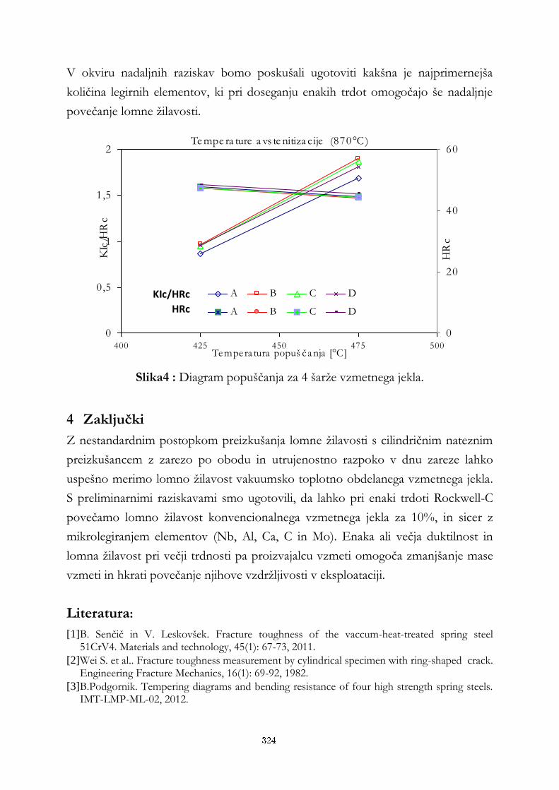
V okviru nadaljnih raziskav bomo poskušali ugotoviti kakšna je najprimernejša
količina legirnih elementov, ki pri doseganju enakih trdot omogočajo še nadaljnje
povečanje lomne žilavosti.
Te mpe ra ture a vs te nitiza cije (870°C)
0
0,5
1
1,5
2
400 425 450 475 500Tempera tura popuš čanja [°C]
KIc
/HR
c
0
20
40
60
HR
c
A B C D
A B C D
KIc/HRc
HRc
Slika4 : Diagram popuščanja za 4 šarže vzmetnega jekla.
4 Zaključki
Z nestandardnim postopkom preizkušanja lomne žilavosti s cilindričnim nateznim
preizkušancem z zarezo po obodu in utrujenostno razpoko v dnu zareze lahko
uspešno merimo lomno žilavost vakuumsko toplotno obdelanega vzmetnega jekla.
S preliminarnimi raziskavami smo ugotovili, da lahko pri enaki trdoti Rockwell-C
povečamo lomno žilavost konvencionalnega vzmetnega jekla za 10%, in sicer z
mikrolegiranjem elementov (Nb, Al, Ca, C in Mo). Enaka ali večja duktilnost in
lomna žilavost pri večji trdnosti pa proizvajalcu vzmeti omogoča zmanjšanje mase
vzmeti in hkrati povečanje njihove vzdržljivosti v eksploataciji.
Literatura:
[1] B. Senčič in V. Leskovšek. Fracture toughness of the vaccum-heat-treated spring steel 51CrV4. Materials and technology, 45(1): 67-73, 2011.
[2] Wei S. et al.. Fracture toughness measurement by cylindrical specimen with ring-shaped crack. Engineering Fracture Mechanics, 16(1): 69-92, 1982.
[3] B.Podgornik. Tempering diagrams and bending resistance of four high strength spring steels. IMT-LMP-ML-02, 2012.
324
Za širši interes
V avtomobilski industriji se za izdelavo listnatih vzmeti uporablja predvsem
vzmetno jeklo 51CrV4. Zaradi stalnega trenda po zmanjševanju mase komponent
potrebujejo proizvajalci vzmeti jekla z izrednimi mehanskimi lastnostmi, med
katerimi je zaradi želene dolge življenjske dobe vzmeti še posebej pomembna
lomna žilavost.
Namen raziskovalne naloge je bil, da raziščemo vpliv vsebnosti različnih legirnih
elementov na lomno žilavost vzmetnega jekla 51CrV, ki smo jo merili z
nestandardnim postopkom preizkušanja lomne žilavosti s cilindričnim nateznim
preizkušancem z zarezo po obodu in utrujenostno razpoko v dnu zareze
preizkušanca, ki je bil vakuumsko toplotno obdelan.
Izdelano je bilo več vzmetnih jekel z različnimi dodatki Nb, Mo, C, Al in Ca.
Na osnovi meritev lomne žilavosti in izdelanega diagrama popuščanja smo
ugotovili, da lahko izboljšamo lomno žilavost klasičnega vzmetnega jekla za 10% že
z majhnimi spremembami vsebnosti legirnih elementov (dodatek 0,075 ut.% Nb ali
zmanjšanje vsebnosti Al za 0,007 ut.% in Ca za 0,0013 ut.%).
325
Dielectric and ferroelectric properties of sol-gel-derived Na0.5Bi0.5TiO3 thin films
Tina Šetinc1,2, Matjaž Spreitzer1, Špela Kunej
1, Danilo Suvorov
1,2
1 Advanced Materials Department, Jožef Stefan Institute, Ljubljana, Slovenia
2 Jožef Stefan International Postgraduate School, Ljubljana, Slovenia
Abstract. Na0.5Bi0.5TiO3 thin films were fabricated on Pt/Ti/SiO2/Si
substrates using a chemical solution deposition (CSD). The decomposition
behaviour of the precursors, the phase formation and the film morphologies
were investigated by means of the thermogravimetric and differential thermal
analysis (TG/DTA) coupled with an online evolved-gas analysis (EGA), X-ray
powder diffraction (XRD), field-emission scanning electron microscopy
(FEG-SEM) and atomic force microscopy (AFM), respectively. The prepared
thin films were single phase with a polycrystalline structure. The measured
room-temperature dielectric constant at 100 kHz was 680, with a
corresponding dielectric loss of 0.06. The temperature dependence of the
dielectric properties showed a steady increase of the permittivity with
increasing temperature, reaching a value of 940 at 200°C.
Keywords: sodium bismuth titanate, chemical solution deposition, thin films,
dielectric properties
1. Introduction
In recent decades much attention has been given to perovskite materials, from both
the theoretical and application points of view, because of their interesting electrical
properties. The dielectric, ferroelectric, piezoelectric, and pyroelectric properties of
these materials were investigated for the corresponding electronic applications,
such as electromechanical devices, transducers, capacitors, actuators, high-k
dielectrics, dynamic random-access memories, field-effect transistors, and logic
circuitry. Ferroelectric thin films, in particular, received a considerable interest due
to their potential integration with microelectronic circuits, offering low operating
voltages, high switching speeds and a possible integration with the existing
semiconductor technology [1-8].
326
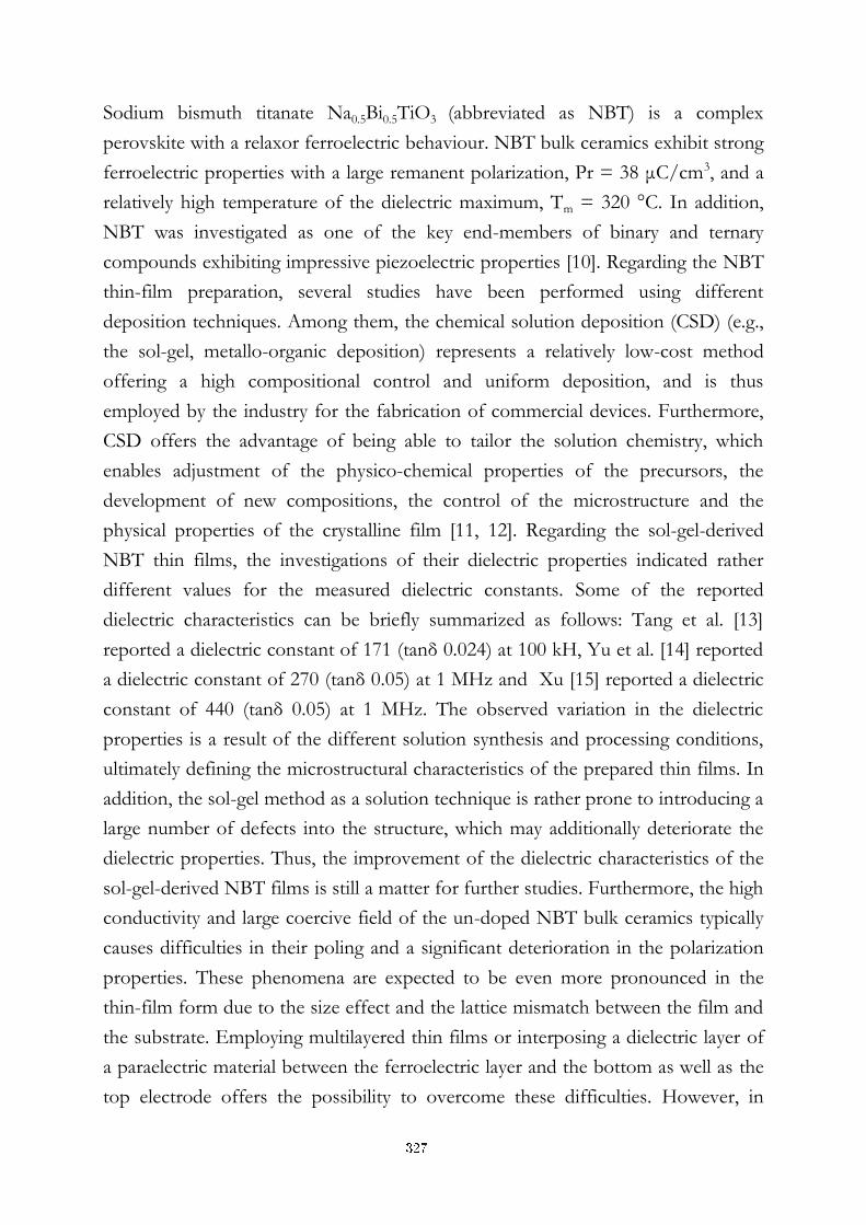
Sodium bismuth titanate Na0.5Bi0.5TiO3 (abbreviated as NBT) is a complex
perovskite with a relaxor ferroelectric behaviour. NBT bulk ceramics exhibit strong
ferroelectric properties with a large remanent polarization, Pr = 38 μC/cm3, and a
relatively high temperature of the dielectric maximum, Tm = 320 °C. In addition,
NBT was investigated as one of the key end-members of binary and ternary
compounds exhibiting impressive piezoelectric properties [10]. Regarding the NBT
thin-film preparation, several studies have been performed using different
deposition techniques. Among them, the chemical solution deposition (CSD) (e.g.,
the sol-gel, metallo-organic deposition) represents a relatively low-cost method
offering a high compositional control and uniform deposition, and is thus
employed by the industry for the fabrication of commercial devices. Furthermore,
CSD offers the advantage of being able to tailor the solution chemistry, which
enables adjustment of the physico-chemical properties of the precursors, the
development of new compositions, the control of the microstructure and the
physical properties of the crystalline film [11, 12]. Regarding the sol-gel-derived
NBT thin films, the investigations of their dielectric properties indicated rather
different values for the measured dielectric constants. Some of the reported
dielectric characteristics can be briefly summarized as follows: Tang et al. [13]
reported a dielectric constant of 171 (tanδ 0.024) at 100 kH, Yu et al. [14] reported
a dielectric constant of 270 (tanδ 0.05) at 1 MHz and Xu [15] reported a dielectric
constant of 440 (tanδ 0.05) at 1 MHz. The observed variation in the dielectric
properties is a result of the different solution synthesis and processing conditions,
ultimately defining the microstructural characteristics of the prepared thin films. In
addition, the sol-gel method as a solution technique is rather prone to introducing a
large number of defects into the structure, which may additionally deteriorate the
dielectric properties. Thus, the improvement of the dielectric characteristics of the
sol-gel-derived NBT films is still a matter for further studies. Furthermore, the high
conductivity and large coercive field of the un-doped NBT bulk ceramics typically
causes difficulties in their poling and a significant deterioration in the polarization
properties. These phenomena are expected to be even more pronounced in the
thin-film form due to the size effect and the lattice mismatch between the film and
the substrate. Employing multilayered thin films or interposing a dielectric layer of
a paraelectric material between the ferroelectric layer and the bottom as well as the
top electrode offers the possibility to overcome these difficulties. However, in
327
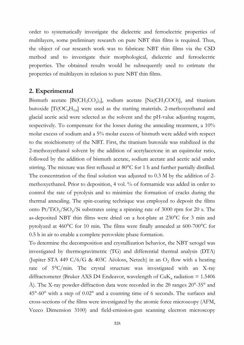
order to systematically investigate the dielectric and ferroelectric properties of
multilayers, some preliminary research on pure NBT thin films is required. Thus,
the object of our research work was to fabricate NBT thin films via the CSD
method and to investigate their morphological, dielectric and ferroelectric
properties. The obtained results would be subsequently used to estimate the
properties of multilayers in relation to pure NBT thin films.
2. Experimental
Bismuth acetate [Bi(CH3CO2)3], sodium acetate [Na(CH3COO)], and titanium
butoxide [Ti(OC4H9)4] were used as the starting materials. 2-methoxyethanol and
glacial acetic acid were selected as the solvent and the pH-value adjusting reagent,
respectively. To compensate for the losses during the annealing treatment, a 10%
molar excess of sodium and a 5% molar excess of bismuth were added with respect
to the stoichiometry of the NBT. First, the titanium butoxide was stabilized in the
2-methoxyethanol solvent by the addition of acetylacetone in an equimolar ratio,
followed by the addition of bismuth acetate, sodium acetate and acetic acid under
stirring. The mixture was first refluxed at 80°C for 1 h and further partially distilled.
The concentration of the final solution was adjusted to 0.3 M by the addition of 2-
methoxyethanol. Prior to deposition, 4 vol. % of formamide was added in order to
control the rate of pyrolysis and to minimize the formation of cracks during the
thermal annealing. The spin-coating technique was employed to deposit the films
onto Pt/TiO2/SiO2/Si substrates using a spinning rate of 3000 rpm for 20 s. The
as-deposited NBT thin films were dried on a hot-plate at 230°C for 3 min and
pyrolyzed at 460°C for 10 min. The films were finally annealed at 600-700°C for
0.5 h in air to enable a complete perovskite phase formation.
To determine the decomposition and crystallization behavior, the NBT xerogel was
investigated by thermogravimetric (TG) and differential thermal analysis (DTA)
(Jupiter STA 449 C/6/G & 403C Aëoloss, Netzch) in an O2 flow with a heating
rate of 5°C/min. The crystal structure was investigated with an X-ray
diffractometer (Bruker AXS D4 Endeavor, wavelength of CuKα radiation = 1.5406
Å). The X-ray powder-diffraction data were recorded in the 2θ ranges 20°-35° and
45°-60° with a step of 0.02° and a counting time of 6 seconds. The surfaces and
cross-sections of the films were investigated by the atomic force microscopy (AFM,
Veeco Dimension 3100) and field-emission-gun scanning electron microscopy
328
(FEG-SEM, Jeol F7600). The electrical measurements were carried out using the
metal-insulator-metal, parallel-plate, capacitor configuration. For the dielectric
characterization, Au electrodes (diameter of 200 μm) were sputtered onto the film
surface through a designed mask. The dielectric properties were characterized in
the frequency range from 1 kHz to 1 MHz using an ac voltage of 1V and an LCR
meter (Agilent 4284A) connected to a Probe Station Cascade Summit 1200 AP.
The out-of-plane dielectric constant was calculated from the capacitance,
C=ε0εrA/d, where d is the film thickness estimated from the cross-section FEG-
SEM images. The polarization-electric field (P-E) hysteresis curves were measured
at room temperature using a radiant precision workstation based on a standard
Sawyer-Tower circuit at 10 Hz.
3. Results and discussion
The thermal decomposition of the NBT xerogel was studied in order to roughly
determine the appropriate temperatures for the thermal treatment of the wet films.
From the corresponding TG/DTA curves, shown in Figure 1, a strong exothermic
peak was observed at a temperature of 329°C, which is related to the formation of
the carboxylate-alkoxide network. The second, relatively weak, exothermic peak at
472°C was ascribed to the crystallization of the NBT. The low temperature of the
decomposition and nucleation was previously observed for NBT films prepared via
the 2-methoxyethanol route. According to the results of the thermal analysis, the
temperature of the drying and the thermolysis were set to 230°C and 460°C,
respectively.
For a complete crystallization to the perovskite phase the films were further
annealed at 600°C and 700°C for 0.5 h and the corresponding diffraction patterns
are shown in Figure 2. Within the measurement precision of the XRD, a single
NBT perovskite phase was determined. The rhombohedral structure of the NBT
can be represented as a pseudo-cubic lattice for simplicity and in such a way it was
possible to index the XRD patterns. The diffraction patterns indicate the
polycrystalline nature of the prepared films with a slight (100) preferential
orientation observed with respect to the reference PDF card (No. 89-3109) [27].
The comparable intensity of the films annealed at different temperatures indicates
that the NBT films are already well crystallized at 600°C.
329
Figure 1: DTA/TG curve of the NBT xerogel.
Figure 2: XRD patterns of the NBT thin films annealed at 600°C and 700°C for
0.5 h.
330
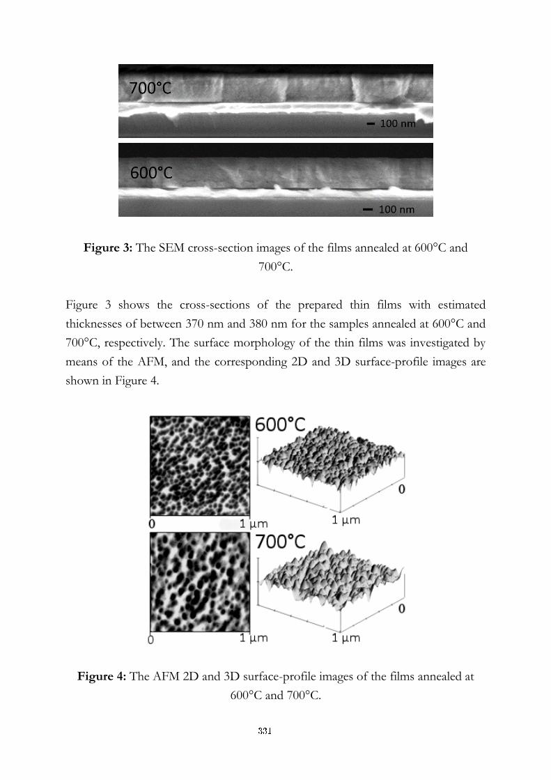
Figure 3: The SEM cross-section images of the films annealed at 600°C and
700°C.
Figure 3 shows the cross-sections of the prepared thin films with estimated
thicknesses of between 370 nm and 380 nm for the samples annealed at 600°C and
700°C, respectively. The surface morphology of the thin films was investigated by
means of the AFM, and the corresponding 2D and 3D surface-profile images are
shown in Figure 4.
Figure 4: The AFM 2D and 3D surface-profile images of the films annealed at
600°C and 700°C.
331
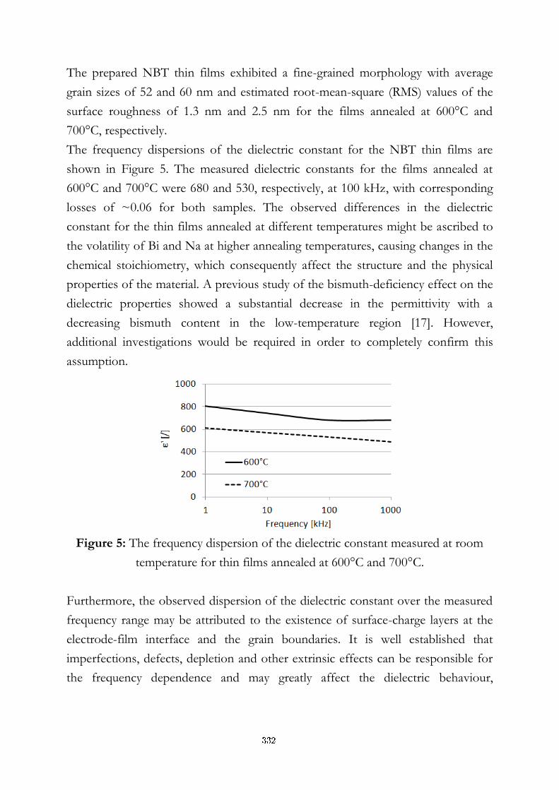
The prepared NBT thin films exhibited a fine-grained morphology with average
grain sizes of 52 and 60 nm and estimated root-mean-square (RMS) values of the
surface roughness of 1.3 nm and 2.5 nm for the films annealed at 600°C and
700°C, respectively.
The frequency dispersions of the dielectric constant for the NBT thin films are
shown in Figure 5. The measured dielectric constants for the films annealed at
600°C and 700°C were 680 and 530, respectively, at 100 kHz, with corresponding
losses of ~0.06 for both samples. The observed differences in the dielectric
constant for the thin films annealed at different temperatures might be ascribed to
the volatility of Bi and Na at higher annealing temperatures, causing changes in the
chemical stoichiometry, which consequently affect the structure and the physical
properties of the material. A previous study of the bismuth-deficiency effect on the
dielectric properties showed a substantial decrease in the permittivity with a
decreasing bismuth content in the low-temperature region [17]. However,
additional investigations would be required in order to completely confirm this
assumption.
Figure 5: The frequency dispersion of the dielectric constant measured at room
temperature for thin films annealed at 600°C and 700°C.
Furthermore, the observed dispersion of the dielectric constant over the measured
frequency range may be attributed to the existence of surface-charge layers at the
electrode-film interface and the grain boundaries. It is well established that
imperfections, defects, depletion and other extrinsic effects can be responsible for
the frequency dependence and may greatly affect the dielectric behaviour,
332
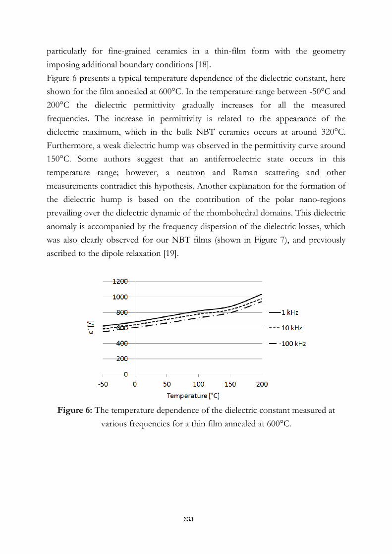
particularly for fine-grained ceramics in a thin-film form with the geometry
imposing additional boundary conditions [18].
Figure 6 presents a typical temperature dependence of the dielectric constant, here
shown for the film annealed at 600°C. In the temperature range between -50°C and
200°C the dielectric permittivity gradually increases for all the measured
frequencies. The increase in permittivity is related to the appearance of the
dielectric maximum, which in the bulk NBT ceramics occurs at around 320°C.
Furthermore, a weak dielectric hump was observed in the permittivity curve around
150°C. Some authors suggest that an antiferroelectric state occurs in this
temperature range; however, a neutron and Raman scattering and other
measurements contradict this hypothesis. Another explanation for the formation of
the dielectric hump is based on the contribution of the polar nano-regions
prevailing over the dielectric dynamic of the rhombohedral domains. This dielectric
anomaly is accompanied by the frequency dispersion of the dielectric losses, which
was also clearly observed for our NBT films (shown in Figure 7), and previously
ascribed to the dipole relaxation [19].
Figure 6: The temperature dependence of the dielectric constant measured at
various frequencies for a thin film annealed at 600°C.
333
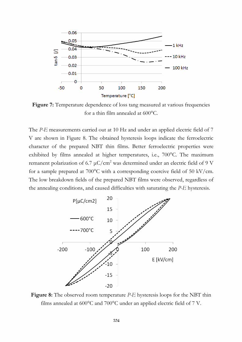
Figure 7: Temperature dependence of loss tang measured at various frequencies
for a thin film annealed at 600°C.
The P-E measurements carried out at 10 Hz and under an applied electric field of 7
V are shown in Figure 8. The obtained hysteresis loops indicate the ferroelectric
character of the prepared NBT thin films. Better ferroelectric properties were
exhibited by films annealed at higher temperatures, i.e., 700°C. The maximum
remanent polarization of 6.7 μC/cm2 was determined under an electric field of 9 V
for a sample prepared at 700°C with a corresponding coercive field of 50 kV/cm.
The low breakdown fields of the prepared NBT films were observed, regardless of
the annealing conditions, and caused difficulties with saturating the P-E hysteresis.
Figure 8: The observed room temperature P-E hysteresis loops for the NBT thin
films annealed at 600°C and 700°C under an applied electric field of 7 V.
334
4. Conclusions
Polycrystalline NBT thin films were prepared on Pt/Ti/SiO2/Si substrates using
the sol-gel method. The NBT thin films exhibited a fine-grained microstructure
with average grain sizes of 52 and 60 nm, and a surface roughness of 1.3 nm and
2.5 nm, for the films annealed at 600°C and 700°C, respectively. In the measured
frequency range from 1 kHz to 1 MHz, the dielectric permittivity ranged from 800
to 630 for the film annealed at 600°C and from 610 to 490 when annealing at
700°C. In the temperature range between -50°C and 200°C the dielectric
permittivity gradually increases for all the measured frequencies, reaching a value of
940 at 200°C for a film annealed at 600°C. Better ferroelectric properties were
measured for the NBT films annealed at 700°C, with a measured remanent
polarization and coercive field of 6.7 μC/cm2 and 50 kV/cm, respectively. The low
breakdown field caused difficulties with obtaining a well-saturated P-E hysteresis
for the prepared NBT thin films, which might be improved by employing
multilayered thin films. This issue will be addressed in our future studies.
References [1] Hill, N. A. J. Phys. Chem. B 2000, 104, 6694. [2] Scott, J. F. Ferroelectr. Rev. 1998, 1, 1. [3] Millis, A. J. Nature 1998, 392, 147. [4] Chandler, C. D.; Roger, C.; Hampden-Smith, M. J. Chem. Rev. 1993, 93, 1205. [5] Schrott, A. G.; Misewich, J. A.; Nagarajan, V.; Ramesh, R. Appl. Phys. Lett. 2003, 82, 4770. [6] Tao, S.; Irvine, J. T. S. Nat. Mater. 2003, 2, 320. [7] G.V. Belokopytov, Ferroelectrics, 168,69 (1995). [8] S. Gevorgian and E. Kollberg, IEEE Trans. Microwave Theory Tech. 49, 2117 (2001). [9] A. Safari and M. Abazari, ‘Lead-free Piezoceramic ceramics and Thin Films,’ IEEE Trans.
Ultrason. Ferroelectr. Freq. Control, 57 [10], 2165-2176 (2010). [14] S.B. Krupanidhi, H. Hu and V. Kumar, J. Appl. Phys. 71 (1992) 376. [15] L.H. Parker and A.F. Tasch, IEEE Circ. Dev. Mag. 1 (1990) 17. [16] A. Mansingh, Ferroelectrics 102 (1990) 69. [17] R. W. Schwartz, T. Schneller, and R. Waser, “Chemical Solution Deposition of Electronic
Oxide Films,” Chimie 7 [5] 433–61 (2004). [18] L. G. Hubert-Pfalzgraf, “Some Trends in the Design of Homo- and Heterometallic
Molecular Precursors of High-Tech Oxides,” Inorg. Chem. Com., 6, 102–20 (2003). [19] K. Kato, K. Suzuki, D. S. Fu, K. Nishizawa, and T. Miki, “Chemical Approach Using
Tailored Liquid Sources for Traditional and Novel Ferroelectric Thin Films,” Jpn. J. Appl. Phys., Part 1, 41 [11B] 6829–35 (2002).
[20] M. L. Calzada, I. Bretos, R. Jiménez, H. Guillon, and L. Pardo, “Low-Temperature Processing of Ferroelectric Thin Films Compatible with Silicon Integrated Circuit Technology,” Adv. Mater., 18 [16] 1620–4 (2004).
335

[21] I. Bretos, R. Jiménez, J. García-López, L. Pardo, and M. L. Calzada, “Photochemical Solution Deposition of Lead-Based Ferroelectric Films: Avoiding the PbO-Excess Addition at Last,” Chem. Mater., 20, 5731–3 (2008).
[22] Tang et al., Chem. Mater., Vol 16, No. 25, 2004 [23] C.Y. Kim, J. Sol-Gel Sci. Tech. (2010), 55:306-310 [24] T. Yu, Thin Solid Films (2007) Volume: 515, Issue: 7-8, Pages: 3563-3566 [25] J. Xu, J. Appl. Phys. 104, 116101 (2008) [26] Yang CH, Journal of Crystal Growth, Volume 284, Issues 1–2, 15 October 2005, Pages 136–141 [27] A.I. Agranovskaya, Izv. Akad. Nauk SSSR, Ser. Fiz., 24, 1275 (1960) [28] J. Suchanicz, The low-frequency dielectric relaxation Na0.5Bi0.5TiO3 ceramics, Materials
Science and Engineering: B Vol. 55, Issues 1–2, 14 August 1998, Pages 114–118 [29] Q. Xu, Y.H. Huang, M.Chen, B.H. Kim, B.K. Ahn, J. Phys. And Chem. Of Solids 69 (2008)
1996-2003 [30] D. Damjanovic, Ferroelectric, dielectric and piezoelectric properties of ferroelectric thin
films and ceramics, Rep- Prog. Phys. 61 (1998) 1267-1324
336
For wider interest
Perovskite materials have attracted a lot of attention over recent decades owing to
their many interesting properties, especially from the application point of view. The
uses of these materials are based on their intrinsic dielectric, ferroelectric,
piezoelectric, and pyroelectric properties in the corresponding electronic devices,
such as micro-electromechanical systems (MEMS), transducers, capacitors,
actuators, high-k dielectrics, dynamic random-access memories, field-effect
transistors, and logic circuitry. Furthermore, a considerable amount of interest in
ferroelectric thin films has resulted from the possibility of integrating them with
existing semiconductor technology, low operating voltages and high switching.
Among the different film-deposition techniques, chemical solution deposition
(CSD) methods (e.g., sol-gel, metallo-organic deposition) are low-cost techniques
that provide high compositional control and uniform deposition, used in industry
for the fabrication of commercial devices with a planar configuration.
The relaxor ferroelectric Na0.5Bi0.5TiO3 (abbreviated as NBT) has attracted
increasing interest as a member of the dielectric perovskites with intriguing
piezoelectric and ferroelectric properties. The distorted NBT structure exhibits
good ferroelectric properties, with a large remanent polarization, Pr = 38 μC/cm3,
and a relatively high temperature of the dielectric maximum, Tm = 320 °C, and was
widely investigated as one of the key end-member compounds for lead-free
piezoelectric ceramics. The main drawbacks of pure NBT are a large coercive field
and a high conductivity, which causes problems in the process of poling. These
phenomena are expected to be even more pronounced in the thin-film form due to
the size effect and the lattice mismatch between the film and the substrate.
Employing multilayered thin films or interposing a dielectric layer of a para-electric
material between the ferroelectric layer and the bottom as well as top electrode
offers a possibility to overcome these difficulties. However, in order to
systematically investigate the dielectric and ferroelectric properties of multilayers
some preliminary research on pure NBT thin films is required. Thus, the object of
our research work was to fabricate the NBT thin films via the CSD method, and to
investigate their morphological, dielectric and ferroelectric properties. The obtained
results would be subsequently used for critically estimating the properties of
multilayers in relation to pure NBT thin films.
337
Synthesis and characterization of calcium phosphate coatings on ZrO2 ceramics for bone implant applications
Martin Štefanič1, Kristoffer Krnel1, Tomaž Kosmač1,2
1 Engineering Ceramics Department, Jožef Stefan Institute, Ljubljana, Slovenia
2 Center of Excellence Namaste, Ljubljana, Slovenia
Abstract. Calcium phosphate (Ca-P) coatings on zirconia bone implants have
a great potential to improve the osseointegration of already existing ceramic
implants, owing to their bone-bonding ability and high osteoconductive
characteristics. In our study, we have prepared three different kinds of Ca-P
coatings, namely the octacalcium phosphate (OCP), hydroxyapatite (HAp) and
β-tricalcium phosphate (β-TCP) coatings. The OCP coatings were prepared
by utilizing a simple wet-chemical biomimetic procedure, which included
immersion of the implant material in a solution with a similar composition as
the human blood plasma and at physiological conditions. Further heat
treatment of the OCP coatings at 600 ºC and 800 ºC resulted in the formation
of HAp and β-TCP coating, respectively. Beside the changes in the
morphology and crystal structure, the heat treatment also improved the
adhesion of the coating to the ceramic substrate.
Keywords: Zirconia ceramics, bone implant, calcium phosphates, bioactive
coating
Introduction
Zirconia implants are becoming increasingly important in the field of dental
medicine because of their good mechanical properties, biocompatibility, and for
aesthetic reasons [1]. However, zirconia is bioinert and this can lead to a poor
338
fixation of the ceramic implant in the bone [2]. A promising approach to
circumvent this problem is to coat the implants with the thin layers of calcium
phosphates (Ca-P), which are known to be bioactive and osteoconductive, i.e., they
show a good bone-bonding ability and support the bone-tissue ingrowth [2]. A very
promising approach for the preparation of coatings is the so-called biomimetic
method, which includes the immersion of the implant into a supersaturated Ca-P
solution under physiological conditions. This method allows the synthesis of
homogenous coatings with a good surface coverage of materials with complex
shapes. Nevertheless, the drawbacks of the method are the long time of the
synthesis, poor reproducibility and, in particular, poor adhesion of the coating to
the substrate [3]. In this work, we report on the use of a simple wet-chemical
biomimetic process for the deposition of an OCP coating on zirconia ceramics and
on the further thermal processing to produce HAp and b-TCP coatings with an
improved attachment to the substrate.
Materials and Methods
Clean zirconia substrates (Y-TZP) in the form of discs were used as substrates for
the preparation of Ca-P coatings. For the coating process, two different Ca-P
solutions were used: Solution 1 and Solution 2. Their compositions are given in the
Table 1.
Table 1. The ionic composition of the CPS1 and CPS2 in mM
Na+ Ca2+ Cl– PO4
3- pH buffer
Solution-1 7.5 2.5 5.0 2.5 7.4 HCl/TRIS
Solution-2 7.5 2.5 5.0 2.5 7.0 HCl/TRIS
The synthesis procedure included two steps. In the first step, the zirconia substrate
was soaked in a plastic beaker filled with 30 ml of the Solution-1 for 1h at 37 °C. In
the second step, the substrate was transferred from the Solution-1 into the beaker
339
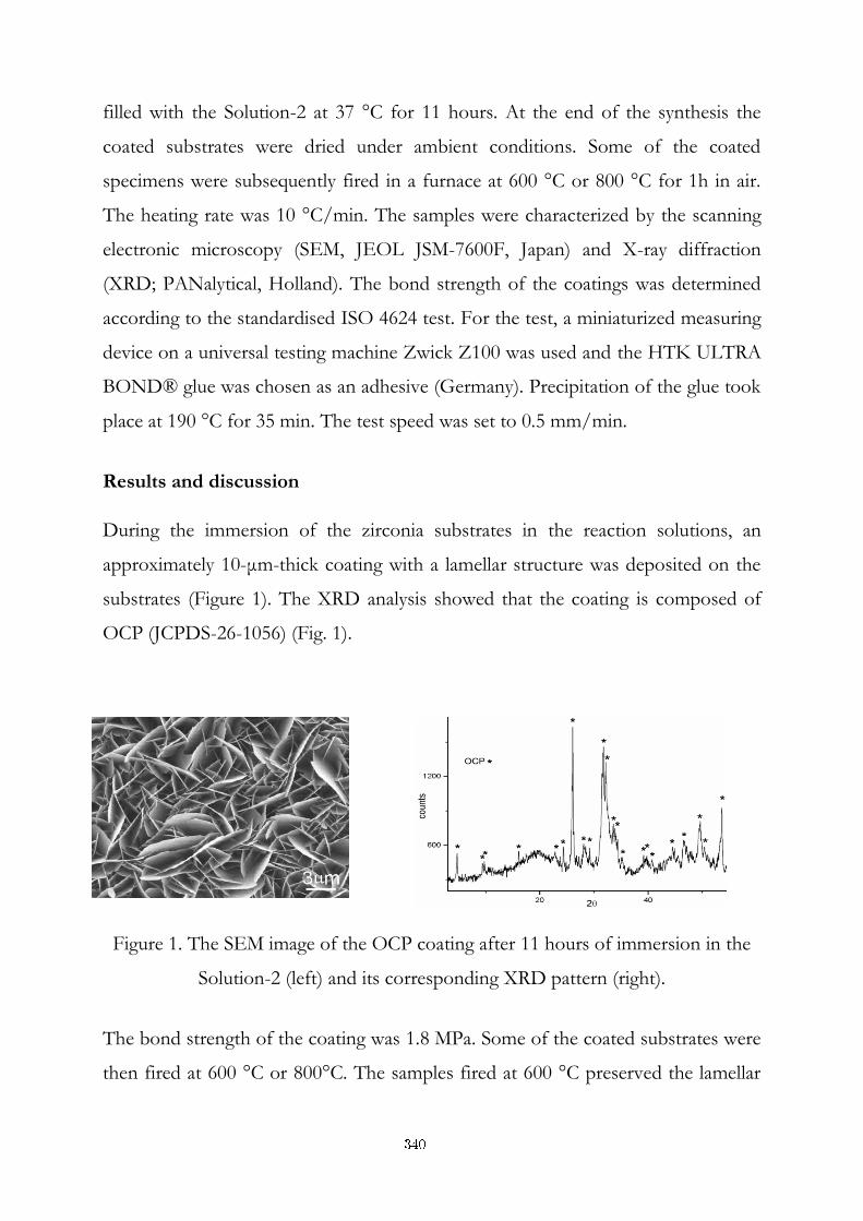
filled with the Solution-2 at 37 °C for 11 hours. At the end of the synthesis the
coated substrates were dried under ambient conditions. Some of the coated
specimens were subsequently fired in a furnace at 600 °C or 800 °C for 1h in air.
The heating rate was 10 °C/min. The samples were characterized by the scanning
electronic microscopy (SEM, JEOL JSM-7600F, Japan) and X-ray diffraction
(XRD; PANalytical, Holland). The bond strength of the coatings was determined
according to the standardised ISO 4624 test. For the test, a miniaturized measuring
device on a universal testing machine Zwick Z100 was used and the HTK ULTRA
BOND® glue was chosen as an adhesive (Germany). Precipitation of the glue took
place at 190 °C for 35 min. The test speed was set to 0.5 mm/min.
Results and discussion
During the immersion of the zirconia substrates in the reaction solutions, an
approximately 10-μm-thick coating with a lamellar structure was deposited on the
substrates (Figure 1). The XRD analysis showed that the coating is composed of
OCP (JCPDS-26-1056) (Fig. 1).
Figure 1. The SEM image of the OCP coating after 11 hours of immersion in the
Solution-2 (left) and its corresponding XRD pattern (right).
The bond strength of the coating was 1.8 MPa. Some of the coated substrates were
then fired at 600 °C or 800°C. The samples fired at 600 °C preserved the lamellar
340
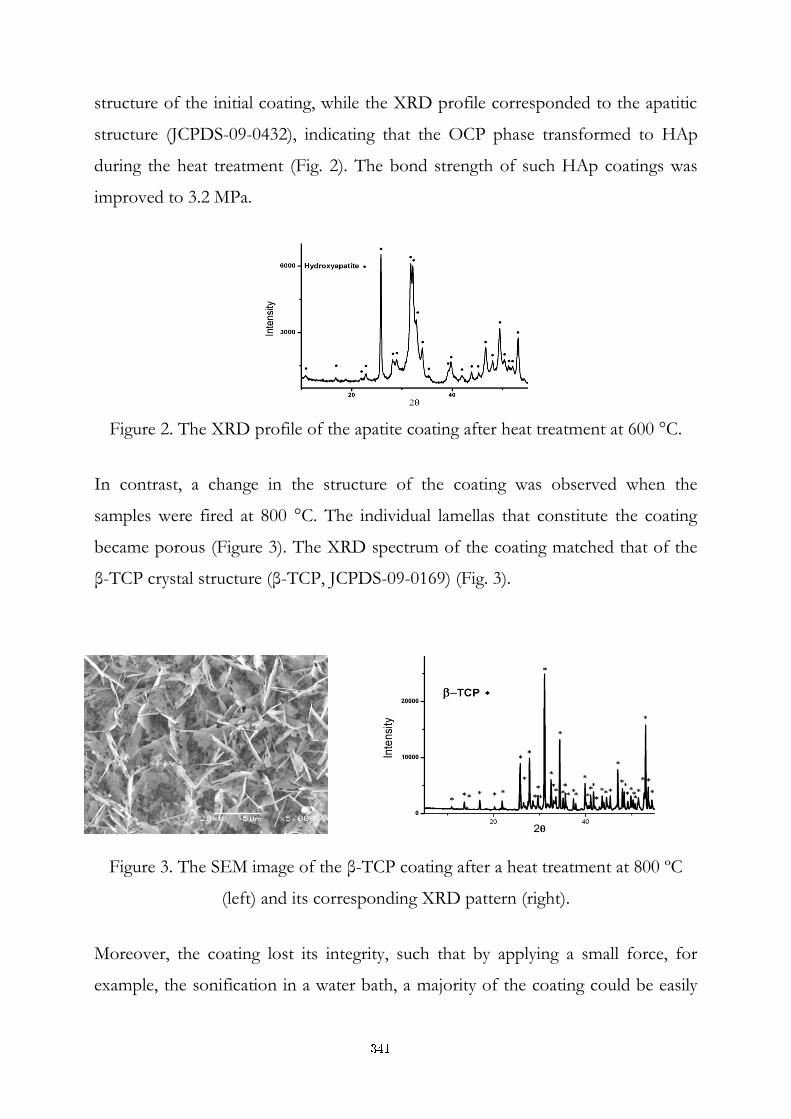
structure of the initial coating, while the XRD profile corresponded to the apatitic
structure (JCPDS-09-0432), indicating that the OCP phase transformed to HAp
during the heat treatment (Fig. 2). The bond strength of such HAp coatings was
improved to 3.2 MPa.
Figure 2. The XRD profile of the apatite coating after heat treatment at 600 °C.
In contrast, a change in the structure of the coating was observed when the
samples were fired at 800 °C. The individual lamellas that constitute the coating
became porous (Figure 3). The XRD spectrum of the coating matched that of the
β-TCP crystal structure (β-TCP, JCPDS-09-0169) (Fig. 3).
Figure 3. The SEM image of the β-TCP coating after a heat treatment at 800 ºC
(left) and its corresponding XRD pattern (right).
Moreover, the coating lost its integrity, such that by applying a small force, for
example, the sonification in a water bath, a majority of the coating could be easily
341
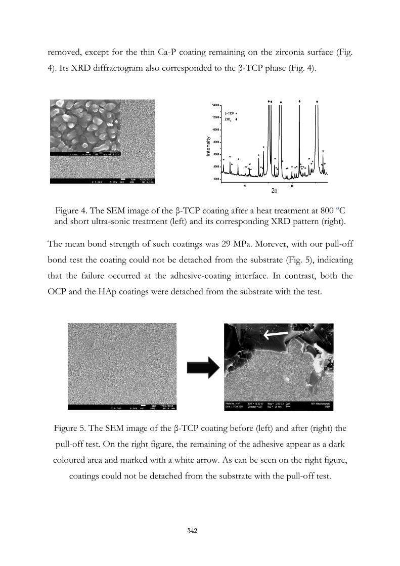
removed, except for the thin Ca-P coating remaining on the zirconia surface (Fig.
4). Its XRD diffractogram also corresponded to the β-TCP phase (Fig. 4).
Figure 4. The SEM image of the β-TCP coating after a heat treatment at 800 ºC and short ultra-sonic treatment (left) and its corresponding XRD pattern (right).
The mean bond strength of such coatings was 29 MPa. Morever, with our pull-off
bond test the coating could not be detached from the substrate (Fig. 5), indicating
that the failure occurred at the adhesive-coating interface. In contrast, both the
OCP and the HAp coatings were detached from the substrate with the test.
Figure 5. The SEM image of the β-TCP coating before (left) and after (right) the
pull-off test. On the right figure, the remaining of the adhesive appear as a dark
coloured area and marked with a white arrow. As can be seen on the right figure,
coatings could not be detached from the substrate with the pull-off test.
342
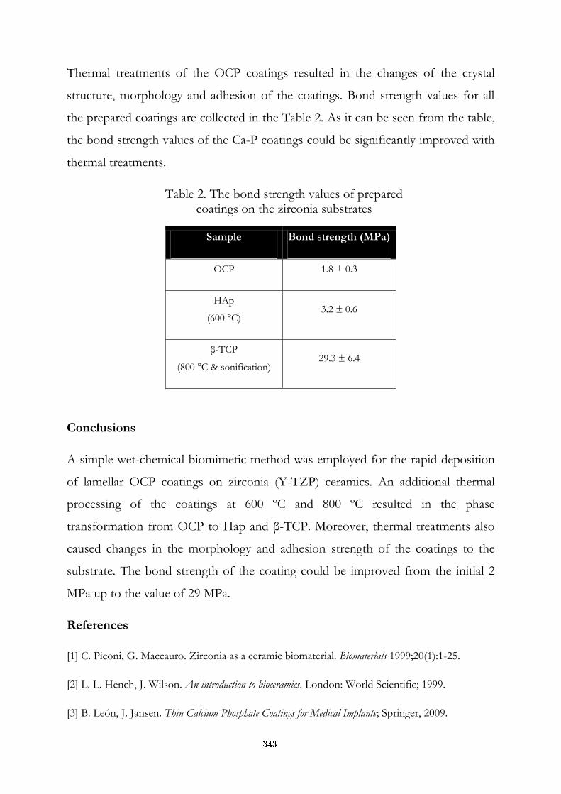
Thermal treatments of the OCP coatings resulted in the changes of the crystal
structure, morphology and adhesion of the coatings. Bond strength values for all
the prepared coatings are collected in the Table 2. As it can be seen from the table,
the bond strength values of the Ca-P coatings could be significantly improved with
thermal treatments.
Table 2. The bond strength values of prepared coatings on the zirconia substrates
Sample Bond strength (MPa)
OCP 1.8 ± 0.3
HAp
(600 °C) 3.2 ± 0.6
β-TCP
(800 °C & sonification) 29.3 ± 6.4
Conclusions
A simple wet-chemical biomimetic method was employed for the rapid deposition
of lamellar OCP coatings on zirconia (Y-TZP) ceramics. An additional thermal
processing of the coatings at 600 ºC and 800 ºC resulted in the phase
transformation from OCP to Hap and β-TCP. Moreover, thermal treatments also
caused changes in the morphology and adhesion strength of the coatings to the
substrate. The bond strength of the coating could be improved from the initial 2
MPa up to the value of 29 MPa.
References
[1] C. Piconi, G. Maccauro. Zirconia as a ceramic biomaterial. Biomaterials 1999;20(1):1-25.
[2] L. L. Hench, J. Wilson. An introduction to bioceramics. London: World Scientific; 1999.
[3] B. León, J. Jansen. Thin Calcium Phosphate Coatings for Medical Implants; Springer, 2009.
343
Za širši interes
Naše raziskovalno delo obsega razvoj metod za pripravo bioaktivnih kalcijevih
fosfatnih (Ca-P) prevlek na keramičnih kostnih implantatih, kot so npr. dentalni,
kolčni in kolenski implantati. Intrinzična lastnost obstoječih implantoloških
materialov je, da se slabo vežejo s kostjo, kar lahko posledično vodi do slabe
fiksacije implantata v kosti, njegovega majanja in izpada. Ca-P imajo edinstveno
lastnost, da v telesu reagirajo s kostjo in se z njo s kemijskimi vezmi čvrsto
povežejo. Tako lahko z nanosom Ca-P prevleke na površino implantata izboljšamo
njegovo fiksacijo v kosti in osteointegracijo. Naša raziskovalna skupina je razvila
preprosto in poceni metodo za sintezo Ca-P prevlek na implantatih. Prevleke imajo
dobre mehanske lastnosti, poleg tega pa nam metoda daje možnost, da
kontroliramo sestavo in morfologijo prevlek. Dodatna prednost našega sinteznega
postopka je, da lahko poteka pri milih pogojih, ki omogoča vključevanje zdravil v
prevleke. Ker so post-operacijske infekcije pogost vzrok za neuspešnost
implantacij, imajo prevleke z vključenimi antibiotiki potencial za izboljšanje
uspešnosti kostnih implantatov.
344
Photocatalytic discoloration of the azo dye methylene blue
in the presence of irradiated TiO2/Pt nano-composite
Vojka Žunič1,2
1 Advanced Materials Department, Jožef Stefan Institute, Ljubljana, Slovenia
2 Jožef Stefan International Postgraduate School, Ljubljana, Slovenia
Abstract. An efficient photocatalytic material TiO2/Pt was prepared via the
sonochemical synthesis followed by the thermal treatment. The TiO2/Pt nano-
composite was able to photocatalytically degrade the azo dye methylene blue
(MB) under UV (ultraviolet) and Vis (visible) irradiation. The enhanced
photocatalytic activity of Pt/TiO2 for methylene blue degradation is attributed
to the following factors; to the presence of Pt particles which store
photogenerated electron thus contribute to an efficient charge carrier’s
separation and to the adsorption of the dye on the surface of the composite,
which acts as a photosensitizer.
Keywords: TiO2 nano-powders, TiO2/Pt nano-composites, photocatalytic
discoloration, methylene blue
1 Introduction
Waste waters originating from industrial discharges represent a global problem
which demands the development of an effective, economic, and environmental
friendly water treatment technology 1. A high environmental impact has the
textile industry since its discharge waters contain large amounts of non-fixed dyes
among which are also the azo dyes 2. It is well known that some of azo dyes and
their degradation products such as aromatic amines are highly carcinogenic 3.
Chemical methods which are able to mineralize organic pollutants to carbon
dioxide, water and inorganics or, at least, transform them into harmless products
are the “advanced oxidation processes” (AOP) 1, 4. One of the AOP is the
heterogeneous photocatalysis, which is based on the generation of highly reactive
and oxidizing hydroxyl radicals in the presence of an irradiated semiconductor
345
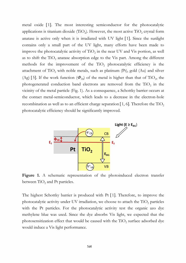
metal oxide 1. The most interesting semiconductor for the photocatalytic
applications is titanium dioxide (TiO2). However, the most active TiO2 crystal form
anatase is active only when it is irradiated with UV light 1. Since the sunlight
contains only a small part of the UV light, many efforts have been made to
improve the photocatalytic activity of TiO2 in the near UV and Vis portion, as well
as to shift the TiO2 anatase absorption edge to the Vis part. Among the different
methods for the improvement of the TiO2 photocatalytic efficiency is the
attachment of TiO2 with noble metals, such as platinum (Pt), gold (Au) and silver
(Ag) 5. If the work function (SB) of the metal is higher than that of TiO2, the
photogenerated conduction band electrons are removed from the TiO2 in the
vicinity of the metal particle (Fig. 1). As a consequence, a Schottky barrier occurs at
the contact metal-semiconductor, which leads to a decrease in the electron-hole
recombination as well as to an efficient charge separation 1, 6. Therefore the TiO2
photocatalytic efficiency should be significantly improved.
Figure 1. A schematic representation of the photoinduced electron transfer
between TiO2 and Pt particles.
The highest Schottky barrier is produced with Pt 1. Therefore, to improve the
photocatalytic activity under UV irradiation, we choose to attach the TiO2 particles
with the Pt particles. For the photocatalytic activity test the organic azo dye
methylene blue was used. Since the dye absorbs Vis light, we expected that the
photosensitization effect that would be caused with the TiO2 surface adsorbed dye
would induce a Vis light performance.
346
2 Experimental
2.1. Synthesis of TiO2/Pt
The TiO2 nano-powders and TiO2/Pt nano-composites were prepared by using an
alkoxide Ti precursor. Titanium(IV) n-butoxide (TNB; TiO4H36C16, 98%) was
dissolved in 1-Bultanol (C4H9OH, 99%) to form a Solution 1. Nitric acid (HNO3,
65%) was diluted in ultrapure water to a form Solution 2. Afterwards a Solution 2
was added dropwise to the Solution 1. A transparent Solution 3 (pH=1) was
formed. The Pt precursor chloroplatinic acid hexahydrate (H2PtCl6·6H2O) was
dissolved in ultrapure water and added to the Solution 3, which was transferred
into a Suslick reactor and heated to the temperature 80°C. Afterwards the
sonication was initiated. The following parameters were used: time of sonication
t=3h, pulse on:off = 02:01 s, amplitude 80%, power P=600W and frequency f=20
kHz. The formed precipitates were separated with centrifugation, dried and
thermally treated in a reducing atmosphere (Ar/H2=96/4) at 400°C for 3h.
2.2. Characterization techniques
The phase composition and the average crystallite size were evaluated utilizing the
X-ray powder diffraction analysis. The specific surface area (sBET) was measured by
the Brunauer-Emmett-Teller method and the morphological characteristics were
analyzed with the transmission electron microscopy (TEM, HRTEM, SAED). UV-
Vis spectra were recorded using a UV-Vis-NIR in which the BaSO4 standard was
used as the reference spectrum. The photocatalytic activity was evaluated in an
aqueous methylene blue solution. A 7.5 ml of the dye solution (2.67 · 10-5 M;
10mg/l) and 15 mg of the TiO2 powder (2g/l) were tested under UV and Vis
irradiation. The change in the absorbance of the dye solution was measured
utilizing the UV-Vis-NIR spectrometer (Shimadzu UV-Vis-NIR 3600).
3 Results and discussion
The phase composition analysis of the TiO2 nano-powder and TiO2/Pt nano-
composite before the thermal treatment revealed that the materials were a semi-
crystalline TiO2 anatase. The following thermal step led to an improvement of
TiO2 crystallinity and to the oxidation state reduction of Pt particles deposited on
the TiO2 surface. The crystallinity and phase composition were also confirmed with
the selected area electron diffraction (SAED) analysis (Fig. 2).
347
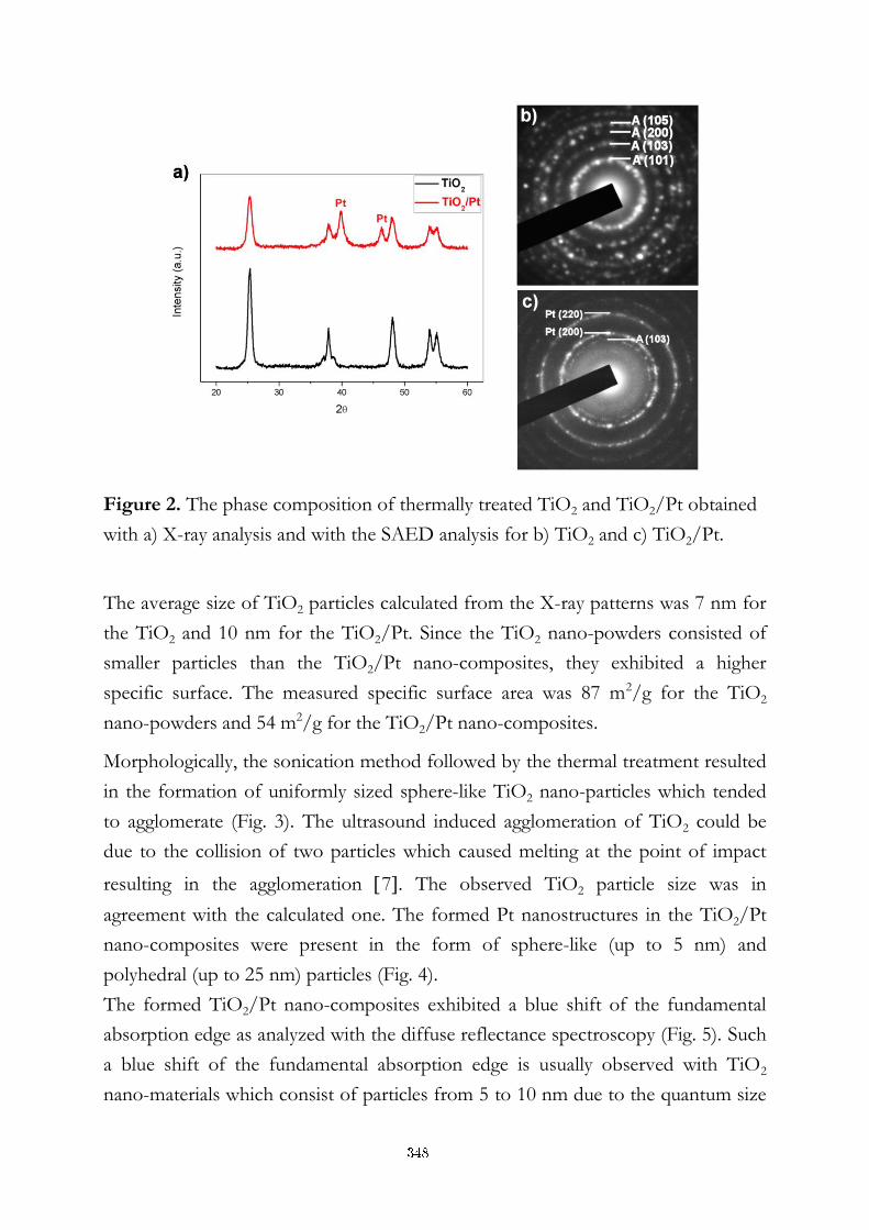
Figure 2. The phase composition of thermally treated TiO2 and TiO2/Pt obtained
with a) X-ray analysis and with the SAED analysis for b) TiO2 and c) TiO2/Pt.
The average size of TiO2 particles calculated from the X-ray patterns was 7 nm for
the TiO2 and 10 nm for the TiO2/Pt. Since the TiO2 nano-powders consisted of
smaller particles than the TiO2/Pt nano-composites, they exhibited a higher
specific surface. The measured specific surface area was 87 m2/g for the TiO2
nano-powders and 54 m2/g for the TiO2/Pt nano-composites.
Morphologically, the sonication method followed by the thermal treatment resulted
in the formation of uniformly sized sphere-like TiO2 nano-particles which tended
to agglomerate (Fig. 3). The ultrasound induced agglomeration of TiO2 could be
due to the collision of two particles which caused melting at the point of impact
resulting in the agglomeration 7. The observed TiO2 particle size was in
agreement with the calculated one. The formed Pt nanostructures in the TiO2/Pt
nano-composites were present in the form of sphere-like (up to 5 nm) and
polyhedral (up to 25 nm) particles (Fig. 4).
The formed TiO2/Pt nano-composites exhibited a blue shift of the fundamental
absorption edge as analyzed with the diffuse reflectance spectroscopy (Fig. 5). Such
a blue shift of the fundamental absorption edge is usually observed with TiO2
nano-materials which consist of particles from 5 to 10 nm due to the quantum size
348
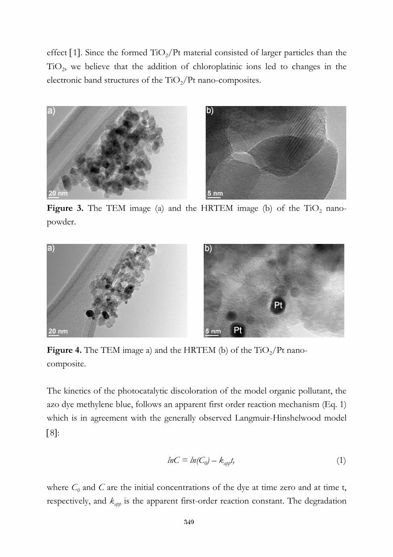
effect 1. Since the formed TiO2/Pt material consisted of larger particles than the
TiO2, we believe that the addition of chloroplatinic ions led to changes in the
electronic band structures of the TiO2/Pt nano-composites.
Figure 3. The TEM image (a) and the HRTEM image (b) of the TiO2 nano-
powder.
Figure 4. The TEM image a) and the HRTEM (b) of the TiO2/Pt nano-
composite.
The kinetics of the photocatalytic discoloration of the model organic pollutant, the
azo dye methylene blue, follows an apparent first order reaction mechanism (Eq. 1)
which is in agreement with the generally observed Langmuir-Hinshelwood model
8:
lnC = ln(C0) – kappt, (1)
where C0 and C are the initial concentrations of the dye at time zero and at time t,
respectively, and kapp is the apparent first-order reaction constant. The degradation
349
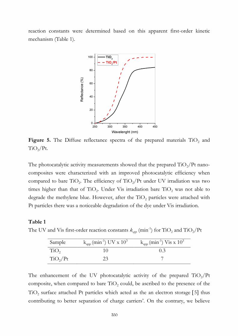
reaction constants were determined based on this apparent first-order kinetic
mechanism (Table 1).
Figure 5. The Diffuse reflectance spectra of the prepared materials TiO2 and
TiO2/Pt.
The photocatalytic activity measurements showed that the prepared TiO2/Pt nano-
composites were characterized with an improved photocatalytic efficiency when
compared to bare TiO2. The efficiency of TiO2/Pt under UV irradiation was two
times higher than that of TiO2. Under Vis irradiation bare TiO2 was not able to
degrade the methylene blue. However, after the TiO2 particles were attached with
Pt particles there was a noticeable degradation of the dye under Vis irradiation.
Table 1
The UV and Vis first-order reaction constants kapp (min-1) for TiO2 and TiO2/Pt
Sample kapp (min-1) UV x 103 kapp (min-1) Vis x 103
TiO2 10 0.3
TiO2/Pt 23 7
The enhancement of the UV photocatalytic activity of the prepared TiO2/Pt
composite, when compared to bare TiO2 could, be ascribed to the presence of the
TiO2 surface attached Pt particles which acted as the an electron storage 5 thus
contributing to better separation of charge carriers’. On the contrary, we believe
350
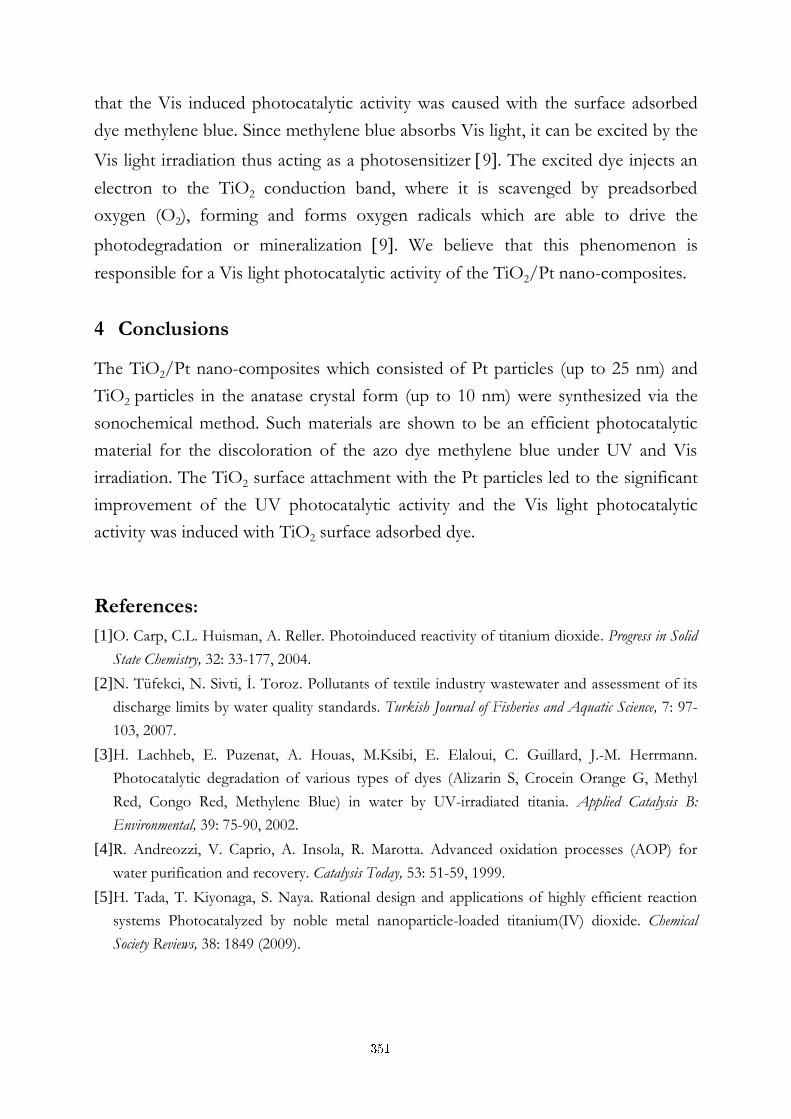
that the Vis induced photocatalytic activity was caused with the surface adsorbed
dye methylene blue. Since methylene blue absorbs Vis light, it can be excited by the
Vis light irradiation thus acting as a photosensitizer 9. The excited dye injects an
electron to the TiO2 conduction band, where it is scavenged by preadsorbed
oxygen (O2), forming and forms oxygen radicals which are able to drive the
photodegradation or mineralization 9. We believe that this phenomenon is
responsible for a Vis light photocatalytic activity of the TiO2/Pt nano-composites.
4 Conclusions
The TiO2/Pt nano-composites which consisted of Pt particles (up to 25 nm) and
TiO2 particles in the anatase crystal form (up to 10 nm) were synthesized via the
sonochemical method. Such materials are shown to be an efficient photocatalytic
material for the discoloration of the azo dye methylene blue under UV and Vis
irradiation. The TiO2 surface attachment with the Pt particles led to the significant
improvement of the UV photocatalytic activity and the Vis light photocatalytic
activity was induced with TiO2 surface adsorbed dye.
References:
[1] O. Carp, C.L. Huisman, A. Reller. Photoinduced reactivity of titanium dioxide. Progress in Solid
State Chemistry, 32: 33-177, 2004.
[2] N. Tüfekci, N. Sivti, İ. Toroz. Pollutants of textile industry wastewater and assessment of its
discharge limits by water quality standards. Turkish Journal of Fisheries and Aquatic Science, 7: 97-
103, 2007.
[3] H. Lachheb, E. Puzenat, A. Houas, M.Ksibi, E. Elaloui, C. Guillard, J.-M. Herrmann.
Photocatalytic degradation of various types of dyes (Alizarin S, Crocein Orange G, Methyl
Red, Congo Red, Methylene Blue) in water by UV-irradiated titania. Applied Catalysis B:
Environmental, 39: 75-90, 2002.
[4] R. Andreozzi, V. Caprio, A. Insola, R. Marotta. Advanced oxidation processes (AOP) for
water purification and recovery. Catalysis Today, 53: 51-59, 1999.
[5] H. Tada, T. Kiyonaga, S. Naya. Rational design and applications of highly efficient reaction
systems Photocatalyzed by noble metal nanoparticle-loaded titanium(IV) dioxide. Chemical
Society Reviews, 38: 1849 (2009).
351

[6] B. Kreaeutler, A.J. Bard. Heterogeneous photocatalytic preparation of supported catalysts.
Photodeposition of platinum on TiO2 powder and other substrates. Journal of the American
chemical society, 100(13): 4317, 1978.
[7] T. Prozorov, R. Prozorov, K.S. Suslick. High velocity interparticle collisions driven by
ultrasound. Journal of American chemical society, 126: 13890 (2004).
[8] R.W. Matthews. Photocatalytic oxidation and adsorption of methylene blue on thin films of
near-ultraviolet-illuminated TiO2. Journal of the Chemical Society, Faraday Transactions, 85(6): 1291
(1989).
[9] T. Wu, T. Lin, J. Zhao, H. Hidaka, N. Serpone. TiO2-assisted photodegradation of dyes. 9.
Photooxidation of a squarylium cyanine dye in aqueous dispersion under visible light
irradiation. Environmental Sciences and Technology, 33: 1379 (1999).
352
For wider interest
It is well know that TiO2 is characterized with photocatalytic properties by utilizing
UV (ultraviolet) light. This phenomena is already been used for commercial
applications such as self-cleaning concrete (Italcement Group) in building facades
(Jubilee Church (also known as the Dives in Misericordia) in Rome) and pavements
(Municipal District of Bergamo, Italy – Borgo Palazzo Street), self-cleaning
windows (Pilkington), ect. Another field, in which the photocatalytic properties of
TiO2 can be of advantage, is the water purification. Water contamination due to the
industrial wastewaters which contain organic dyes has become a global problem.
About 1-20% of organic dyes are lost during the industrial dyeing processes and
released into the environment. The dyes itself and their degradation products
represent toxic substances which cause diverse effects on animal and human health.
Therefore, the purification and remediation of discharged waters generated from
industrial processes is a necessity. Having in mind such problems, the idea of this
work was to prepare TiO2 which could be used for azo dyes degradation in water.
Since the UV light represents only a small part of the sunlight (only 2-3%) the goal
of our work was to synthesize a TiO2 which exhibits improved photocatalytic
properties under UV irradiation and also is active under Vis (visible) light
irradiation. Since such TiO2 is able to degraded organic dyes utilizing solar energy
(UV and Vis) it represents an economic and efficient method for water purification.
We prepared such photocatalyst by forming a TiO2/Pt nano-composite which is
able to effectively photocatalytically degraded the azo dye methylene blue under
UV and Vis irradiation.
353
LIFE TIME ASSESSMENT OF REAL COMPONENTS EXPOSED TO HIGH TEMPERATURES AND PRESURES
Borut Žužek1,2, Bojan Podgornik1, Monika Jenko1
1 Institute of Metals and Technology, Ljubljana, Slovenia
2 Jožef Stefan International Postgraduate School, Ljubljana, Slovenia
Abstract. Components in the industry are often exposed to elevated temperatures
and high pressures. These conditions cause changes in the microstructure and
thermo-mechanical properties of steel components. With the aim to determine the
properties of steels after a certain period of operation, thermo-mechanical
investigations and microstructure characterization can be made and the results of
this investigation can serve for the remaining lifetime assessment of components.
From the economic and technological point of view this is a very important
information.
Creep is one of the major mechanisms which cause the deformation and
degradation of steels at elevated temperatures. The creep can occur in local areas
due to an increased load or due to a microstructural degradation during the
operation at elevated temperatures. The microstructure degradation of the steels can
be defined by microstructural investigations on metallographic samples or replicas.
The aim of this work is to present some methods for the microstructure
characterization of steels used in the Slovenian thermal power plants.
Keywords: lifetime assessment, creep, microstructural degradation, elevated
temperatures
1 Introduction
Elevated temperatures and high pressures are present in a lot of different industrial
applications. High temperatures and pressures accelerate a lot of thermodynamic
processes in steel which cause the degradation of steel. Mechanical properties of
steel are deteriorated trough the thermal degradation of steel with the
microstructural changes, thinning of the wall thickness due to corrosion processes,
354
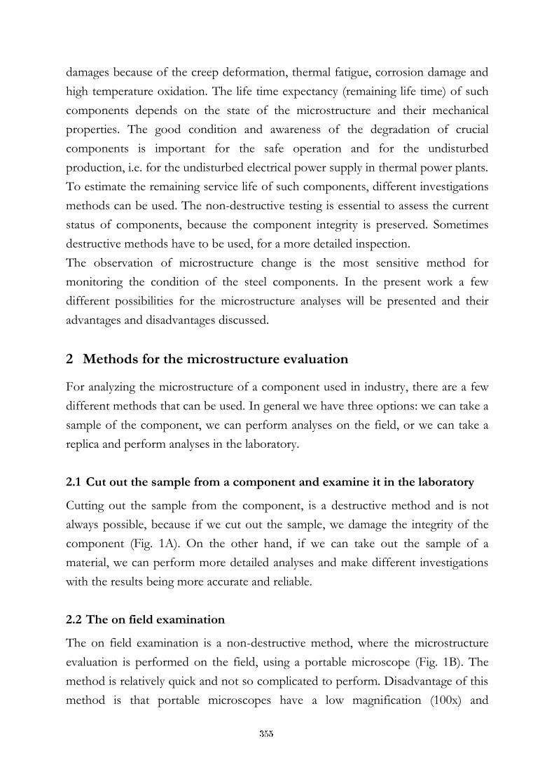
damages because of the creep deformation, thermal fatigue, corrosion damage and
high temperature oxidation. The life time expectancy (remaining life time) of such
components depends on the state of the microstructure and their mechanical
properties. The good condition and awareness of the degradation of crucial
components is important for the safe operation and for the undisturbed
production, i.e. for the undisturbed electrical power supply in thermal power plants.
To estimate the remaining service life of such components, different investigations
methods can be used. The non-destructive testing is essential to assess the current
status of components, because the component integrity is preserved. Sometimes
destructive methods have to be used, for a more detailed inspection.
The observation of microstructure change is the most sensitive method for
monitoring the condition of the steel components. In the present work a few
different possibilities for the microstructure analyses will be presented and their
advantages and disadvantages discussed.
2 Methods for the microstructure evaluation
For analyzing the microstructure of a component used in industry, there are a few
different methods that can be used. In general we have three options: we can take a
sample of the component, we can perform analyses on the field, or we can take a
replica and perform analyses in the laboratory.
2.1 Cut out the sample from a component and examine it in the laboratory
Cutting out the sample from the component, is a destructive method and is not
always possible, because if we cut out the sample, we damage the integrity of the
component (Fig. 1A). On the other hand, if we can take out the sample of a
material, we can perform more detailed analyses and make different investigations
with the results being more accurate and reliable.
2.2 The on field examination
The on field examination is a non-destructive method, where the microstructure
evaluation is performed on the field, using a portable microscope (Fig. 1B). The
method is relatively quick and not so complicated to perform. Disadvantage of this
method is that portable microscopes have a low magnification (100x) and
355
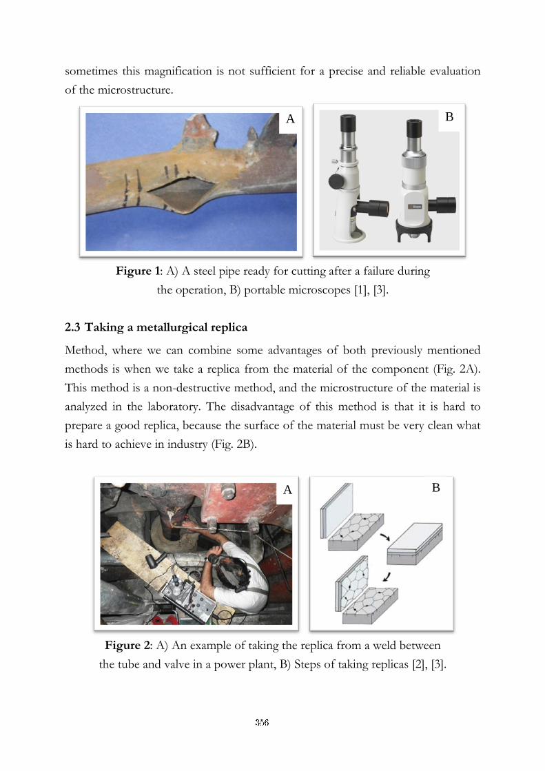
sometimes this magnification is not sufficient for a precise and reliable evaluation
of the microstructure.
Figure 1: A) A steel pipe ready for cutting after a failure during
the operation, B) portable microscopes [1], [3].
2.3 Taking a metallurgical replica
Method, where we can combine some advantages of both previously mentioned
methods is when we take a replica from the material of the component (Fig. 2A).
This method is a non-destructive method, and the microstructure of the material is
analyzed in the laboratory. The disadvantage of this method is that it is hard to
prepare a good replica, because the surface of the material must be very clean what
is hard to achieve in industry (Fig. 2B).
Figure 2: A) An example of taking the replica from a weld between
the tube and valve in a power plant, B) Steps of taking replicas [2], [3].
A B
A B
356
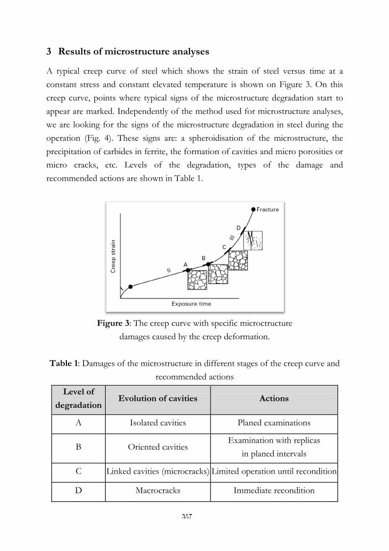
3 Results of microstructure analyses
A typical creep curve of steel which shows the strain of steel versus time at a
constant stress and constant elevated temperature is shown on Figure 3. On this
creep curve, points where typical signs of the microstructure degradation start to
appear are marked. Independently of the method used for microstructure analyses,
we are looking for the signs of the microstructure degradation in steel during the
operation (Fig. 4). These signs are: a spheroidisation of the microstructure, the
precipitation of carbides in ferrite, the formation of cavities and micro porosities or
micro cracks, etc. Levels of the degradation, types of the damage and
recommended actions are shown in Table 1.
Figure 3: The creep curve with specific microctructure
damages caused by the creep deformation.
Table 1: Damages of the microstructure in different stages of the creep curve and
recommended actions
Level of
degradation Evolution of cavities Actions
A Isolated cavities Planed examinations
B Oriented cavities Examination with replicas
in planed intervals
C Linked cavities (microcracks) Limited operation until recondition
D Macrocracks Immediate recondition
357
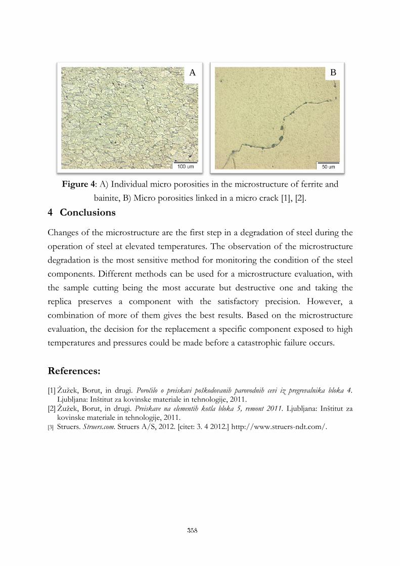
Figure 4: A) Individual micro porosities in the microstructure of ferrite and
bainite, B) Micro porosities linked in a micro crack [1], [2].
4 Conclusions
Changes of the microstructure are the first step in a degradation of steel during the
operation of steel at elevated temperatures. The observation of the microstructure
degradation is the most sensitive method for monitoring the condition of the steel
components. Different methods can be used for a microstructure evaluation, with
the sample cutting being the most accurate but destructive one and taking the
replica preserves a component with the satisfactory precision. However, a
combination of more of them gives the best results. Based on the microstructure
evaluation, the decision for the replacement a specific component exposed to high
temperatures and pressures could be made before a catastrophic failure occurs.
References:
[1] Žužek, Borut, in drugi. Poročilo o preiskavi poškodovanih parovodnih cevi iz pregrevalnika bloka 4. Ljubljana: Inštitut za kovinske materiale in tehnologije, 2011.
[2] Žužek, Borut, in drugi. Preiskave na elementih kotla bloka 5, remont 2011. Ljubljana: Inštitut za kovinske materiale in tehnologije, 2011.
[3] Struers. Struers.com. Struers A/S, 2012. [citet: 3. 4 2012.] http://www.struers-ndt.com/.
A B
358

Za širši interes
V proizvodnih industrijskih obratih je mnogo komponent pogosto izpostavljenih
delu pri visokih temperaturah in delu pod tlakom. Visoka temperatura in povišan
tlak pospešujeta poslabšanje mehanskih lastnosti jekla. Zaradi slabšanja mehanskih
lastnosti jekla med obratovanjem lahko po določenem času pride do nepričakovane
odpovedi kakšne od komponent. Poškodba komponente, ki deluje v okolju visokih
temperatur in tlakov, pa je velikokrat podobna eksploziji bombe.
Zavedanje neprestanega slabšanja mehanskih lastnosti tako izpostavljenih
komponent je iz ekonomskega in tehničnega vidika zelo pomembno. Odpoved
takšne komponente povzroči ustavitev proizvodnje, nedoseganje zastavljenih ciljev
in izpad dohodka, lahko pa tudi nevarnost ogrožanja življenja zaposlenih.
Stanje takšnih komponent lahko preverimo z različnimi metodami metalografske
analize, kjer se pod mikroskopom preveri stanje mikrostrukture jekla.
Metalografske preiskave lahko dopolnimo tudi z drugimi neporušitvenimi
preiskavami, kot so ultrazvočne meritve, preiskave s tekočimi penetranti, meritve
trdote, itd.
Na podlagi teh preiskav lahko ocenimo preostalo življenjsko dobo takšnih
komponent in podamo mnenje o primernosti njihovega nadaljnjega varnega
obratovanja.
359


Organizator
V sodelovanju z
Center odličnosti nanoznanosti
in nanotehnologije
Center odličnosti Napredni nekovinski materiali s tehnologijami prihodnosti
Center odličnosti za integrirane pristope v
kemiji in biotehnologiji proteinov
361

Ustanovitelji in partnerji MPŠ
363


Related Documents


![IV. DOKTORSKA ZNANSTVENORAZISKOVALNA MEDNARODNA … · Zbornik prispevkov [Elektronski vir] = Proceedings / IV. doktorska znanstvenoraziskovalna mednarodna konferenca = IV. Doctoral](https://static.cupdf.com/doc/110x72/60cb72ed1af8e0096c46cf18/iv-doktorska-znanstvenoraziskovalna-mednarodna-zbornik-prispevkov-elektronski.jpg)


