1 Data Mining: Concepts and Techniques — Chapter 3 — Cont. More on Feature Selection: Chi-squared test Principal Component Analysis.

1

Data Mining: Concepts and Techniques

— Chapter 3 —Cont.

More on Feature Selection: Chi-squared test

Principal Component Analysis

2

Attribute Selection

Question: Are attributes A1 and A2 independent? If they are very

dependent, we can remove eitherA1 or A2

If A1 is independent on a class attribute A2, we can remove A1 from our training data

IDOutlo

ok

Temperature

Humidity

Windy

Play

1 100 40 90 0 T

2 100 40 90 1 F

3 50 40 90 0 T

4 10 30 90 0 T

5 10 15 70 0 T

6 10 15 70 1 F

7 50 15 70 1 T

8 100 30 90 0 F

9 100 15 70 0 T

10

10 30 70 0 F

11

100 30 70 1 F

12

50 30 90 1 T

13

50 40 70 0 T

14

10 30 90 1 F

3

Deciding to remove attributes in feature selection

A1

A2=class attribute

A2 = class attribute

Dependent(ChiSq=small)

Independent(Chisq=large

?

?

?

?

Dependent(ChiSq=small)

Independent(Chisq=large

4

Chi-Squared Test (cont.)

Question: Are attributes A1 and A2 independent?

These features are nominal valued (discrete)

Null Hypothesis: we expect independence

Outlook Temperature

Sunny High

Cloudy Low

Sunny High

5

The Weather example: Observed Count

temperature

Outlook

High Low Outlook Subtotal

Sunny 2 0 2

Cloudy 0 1 1

TemperatureSubtotal:

2 1 Total count in table =3

Outlook Temperature

Sunny High

Cloudy Low

Sunny High

6

The Weather example: Expected Count

temperature

Outlook

High Low Subtotal

Sunny 2*2/3=4/3=1.3

2*1/3=2/3=0.6

2

Cloudy 2*1/3=0.6

1*1/3=0.3

1

Subtotal: 2 1 Total count in table =3

If attributes were independent, then the subtotals would be Like this (this table is also known as

Outlook Temperature

Sunny High

Cloudy Low

Sunny High

7

Question: How different between observed and expected?

•If Chi-squared value is very large, then A1 and A2 are not independent that is, they are dependent!

•Degrees of freedom: if table has n*m items, then freedom = (n-1)*(m-1)

•In our example

•Degree = 1

•Chi-Squared=?

8

Chi-Squared Table: what does it mean?

If calculated value is much greater than in the table, then you have reason to reject the independence assumption

When your calculated chi-square value is greater than the chi2 value shown in the 0.05 column (3.84) of this table you are 95% certain that attributes are actually dependent!

i.e. there is only a 5% probability that your calculated X2 value would occur by chance

9

Example Revisited (http://helios.bto.ed.ac.uk/bto/statistics/tress9.html)

We don’t have to have two-dimensional count table (also known as contingency table)

Suppose that the ratio of male to female students in the Science Faculty is exactly 1:1,

But, the Honours class over the past ten years there have been 80 females and 40 males.

Question: Is this a significant departure from the (1:1) expectation?

Observed

Honours

Male Female Total

40 80 120

10

Expected (http://helios.bto.ed.ac.uk/bto/statistics/tress9.html)

Suppose that the ratio of male to female students in the Science Faculty is exactly 1:1,

but in the Honours class over the past ten years there have been 80 females and 40 males.

Question: Is this a significant departure from the (1:1) expectation?

Note: the expected is filled in, from 1:1 expectation, instead of calculated

Expected

Honours

Male Female Total

60 60 120

11

Chi-Squared Calculation

　 Female Male Total

Observed numbers (O)

80 40 120

Expected numbers (E)

60 60 120

O - E 20 -20 0

(O-E)2 400 400 　

(O-E)2 / E 6.67 6.67Sum=13.34 =

X2

12

Chi-Squared Test (Cont.) Then, check the chi-squared table for significance

http://helios.bto.ed.ac.uk/bto/statistics/table2.html#Chi%20squared%20test

Compare our X2 value with a c2 (chi squared) value in a table of c2 with n-1 degrees of freedom

n is the number of categories, i.e. 2 in our case -- males and females).

We have only one degree of freedom (n-1). From the c2 table, we find a "critical value of 3.84 for p = 0.05.

13.34 > 3.84, and the expectation (that the Male:Female in honours major are 1:1) is wrong!

13

Chi-Squared Test in Weka: weather.nominal.arff

@relation weather.symbolic

@attribute outlook {sunny, overcast, rainy}@attribute temperature {hot, mild, cool}@attribute humidity {high, normal}@attribute windy {TRUE, FALSE}@attribute play {yes, no}

@datasunny,hot,high,FALSE,nosunny,hot,high,TRUE,noovercast,hot,high,FALSE,yesrainy,mild,high,FALSE,yesrainy,cool,normal,FALSE,yesrainy,cool,normal,TRUE,noovercast,cool,normal,TRUE,yessunny,mild,high,FALSE,nosunny,cool,normal,FALSE,yesrainy,mild,normal,FALSE,yessunny,mild,normal,TRUE,yesovercast,mild,high,TRUE,yesovercast,hot,normal,FALSE,yesrainy,mild,high,TRUE,no

14

Chi-Squared Test in Weka

15

Chi-Squared Test in Weka

16

Example of Decision Tree Induction

Initial attribute set:{A1, A2, A3, A4, A5, A6}

A4 ?

A1? A6?

Class 1 Class 2 Class 1 Class 2

> Reduced attribute set: {A1, A4, A6}

17

Given N data vectors from k-dimensions, find c <= k orthogonal vectors that can be best used to represent data

The original data set is reduced to one consisting of N data vectors on c principal components (reduced dimensions)

Each data vector Xj is a linear combination of the c principal component vectors Y1, Y2, … Yc

Xj= m+W1*Y1+W2*Y2+…+Wk*Yc, i=1, 2, … N M is the mean of the data set W1, W2, … are the ith components Y1, Y2, … are the ith Eigen vectors

Works for numeric data only Used when the number of dimensions is large

Principal Component Analysis

18

X1

X2

Principal Component AnalysisSee online tutorials such as http://www.cs.otago.ac.nz/cosc453/student_tutorials/principal_components.pdf

Note: Y1 is the first eigen vector, Y2 is the second. Y2 ignorable.

Y1

Y2x

xx x

x

x

xx

x

x

xx

x xx

x

xx

x xx

x

x

x

x

Key observation:variance = largest!

19

Principal Component Analysis: one attribute first

Question: how much spread is in the data along the axis? (distance to the mean)

Variance=Standard deviation^2

Temperature

42

40

24

30

15

18

15

30

15

30

35

30

40

30

)1(

)(1

2

2

n

XXs

n

ii

20

Now consider two dimensions

X=Temperature Y=Humidity

40 90

40 90

40 90

30 90

15 70

15 70

15 70

30 90

15 70

30 70

30 70

30 90

40 70

30 90

)1(

))((

),cov( 1

n

YYXX

YX

n

i

ii

Covariance: measures thecorrelation between X and Y• cov(X,Y)=0: independent•Cov(X,Y)>0: move same dir•Cov(X,Y)<0: move oppo dir

21

More than two attributes: covariance matrix Contains covariance values between all

possible dimensions (=attributes):

Example for three attributes (x,y,z):

)),cov(|( jiijijnxn DimDimccC

),cov(),cov(),cov(

),cov(),cov(),cov(

),cov(),cov(),cov(

zzyzxz

zyyyxy

zxyxxx

C

22

Background: eigenvalues AND eigenvectors

Eigenvectors e : C e = e How to calculate e and :

Calculate det(C-I), yields a polynomial (degree n)

Determine roots to det(C-I)=0, roots are eigenvalues

Check out any math book such as Elementary Linear Algebra by Howard Anton,

Publisher John,Wiley & Sons Or any math packages such as MATLAB

23

Steps of PCA

Let be the mean vector (taking the mean of all rows)

Adjust the original data by the mean X’ = X –

Compute the covariance matrix C of adjusted X

Find the eigenvectors and eigenvalues of C.

X

For matrix C, vectors e (=column vector) having same direction as Ce :

eigenvectors of C is e such that Ce=e,

is called an eigenvalue of C.

Ce=e (C-I)e=0

Most data mining packages do this for you.

X

24

Steps of PCA (cont.)

Calculate eigenvalues and eigenvectors e for covariance matrix:

Eigenvalues j corresponds to variance on each component j

Thus, sort by j Take the first n eigenvectors ei; where n is the number

of top eigenvalues These are the directions with the largest variances

nnnn xx

xx

xx

e

e

e

y

y

y

1

212

111

2

1

1

12

11

.........

25

An Example

X1 X2 X1' X2'

19 63 -5.1 9.25

39 74 14.9 20.25

30 87 5.9 33.25

30 23 5.9 -30.75

15 35 -9.1 -18.75

15 43 -9.1 -10.75

15 32 -9.1 -21.75

30 73 5.9 19.25

0

10

20

30

40

50

60

70

80

90

100

0 10 20 30 40 50

Series1

Mean1=24.1Mean2=53.8

-40

-30

-20

-10

0

10

20

30

40

-15 -10 -5 0 5 10 15 20

Series1

26

Covariance Matrix

C=

Using MATLAB, we find out: Eigenvectors: e1=(-0.98,-0.21), 1=51.8 e2=(0.21,-0.98), 2=560.2 Thus the second eigenvector is more important!

75 106

106 482

27

If we only keep one dimension: e2

We keep the dimension of e2=(0.21,-0.98)

We can obtain the final data as

2121 *98.0*21.098.0

21.0iiiii xxxxy

-0.5

-0.4

-0.3

-0.2

-0.1

0

0.1

0.2

0.3

0.4

0.5

-40 -20 0 20 40

yi

-10.14

-16.72

-31.35

31.374

16.464

8.624

19.404

-17.63

28

Using Matlab to figure it out

29

PCA in Weka

30

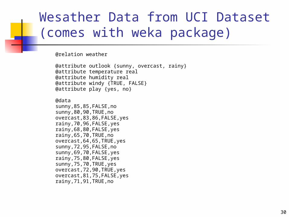
Wesather Data from UCI Dataset (comes with weka package)

@relation weather

@attribute outlook {sunny, overcast, rainy}@attribute temperature real@attribute humidity real@attribute windy {TRUE, FALSE}@attribute play {yes, no}

@datasunny,85,85,FALSE,nosunny,80,90,TRUE,noovercast,83,86,FALSE,yesrainy,70,96,FALSE,yesrainy,68,80,FALSE,yesrainy,65,70,TRUE,noovercast,64,65,TRUE,yessunny,72,95,FALSE,nosunny,69,70,FALSE,yesrainy,75,80,FALSE,yessunny,75,70,TRUE,yesovercast,72,90,TRUE,yesovercast,81,75,FALSE,yesrainy,71,91,TRUE,no

31

PCA in Weka (I)

32

33

Summary of PCA

PCA is used for reducing the number of numerical attributes

The key is in data transformation Adjust data by mean Find eigenvectors for covariance matrix Transform data

Note: only linear combination of data (weighted sum of original data)

34

Missing and Inconsistent values

Linear regression: Data

are modeled to fit a

straight line

least-square method to

fit Y=a+bX Multiple regression: Y = b0

+ b1 X1 + b2 X2. Many nonlinear

functions can be transformed into the above.

XbYa

XX

YYXXb

2)(

))((

35

Regression

Age

Height

y = x + 1

X1

Y1

Y1’

36

Clustering for Outlier detection

Outliers can be incorrect data. Clusters

majority behavior

37

Data Reduction with Sampling

Allow a mining algorithm to run in complexity that is potentially sub-linear to the size of the data

Choose a representative subset of the data Simple random sampling may have very poor

performance in the presence of skew (uneven) classes

Develop adaptive sampling methods Stratified sampling:

Approximate the percentage of each class (or subpopulation of interest) in the overall database

Used in conjunction with skewed data

38

Sampling

SRSWOR

(simple random

sample without

replacement)

SRSWR

Raw Data

39

Sampling Example

Raw Data Cluster/Stratified Sample

40

Summary

Data preparation is a big issue for data mining

Data preparation includes

Data warehousing

Data reduction and feature selection

Discretization

Missing values

Incorrect values

Sampling