1 Conservation Equations. 2 Dynamics We now consider the Dynamics in Computational Fluid Dynamics (CFD). Specifically for WIND: Fluid Dynamics Turbulence.

1

Conservation Equations

2

Dynamics

We now consider the Dynamics in Computational Fluid Dynamics (CFD). Specifically for WIND:

• Fluid Dynamics• Turbulence• Chemical Dynamics• Magneto-Fluid Dynamics

Dynamics involves relating the forces in the system to the properties of the system. Dynamics involves kinematics (geometrical aspects of motion) and kinetics (analysis of forces causing motion).

All of these involve fluid behavior and it is known that conservation principles governs this behavior.

3

Conservation Principles

The dynamics of fluid flow is described by several conservation principles:

• Mass (mass of system and species)• Momentum• Energy (internal, turbulent, chemical)• Magnetism?• Electrical charge?

Fluid motion requires determining the fluid velocity components and additional static properties (p, T, , ci).

v

4

An integral formulation of the conservation statement helps visualize the nature of the conservation:

Q is conserved quantity, scalar or vector (i.e. mass, momentum)

V is the control volume (time-varying)

S is the control surface (time-varying)

is surface normal vector with positive direction out of volume

D is non-convective terms of the flux (vector or tensor)

The control volume can translate and rotate, as well as, change shape and deform. Gauss’ theorem relates control surface and control volume.

Conservation Statement

),(),(),(

ˆtrVtrStrV

dVPdSnQgvdVQdt

d

D

Time-rate of change of Q in the control volume.

Flux of Q leaving the control volume through the control surface.

Production of Q within the control volume.

n̂

5

The dynamics can be expressed in the following equation sets:

Q, D, and P can be scalars or an algebraic vectors with elements as vectors. D can be a vector or dyadic, depending on whether Q is a scalar or vector.

Equations Sets

MFD

chem

turb

NS

Q

Q

Q

Q

Q

MFD

chem

turb

NS

D

D

D

D

D

MFD

chem

turb

NS

P

P

P

P

P

6

Complete Description of Equations

A complete description of the dynamic equations requires:

1. Equations

2. Frame of Reference

3. Control Volume and Control Surface

4. Boundary Conditions

5. Initial Conditions

7

Frames of Reference

Some frames of reference:Inertial Cartesian Frame

Cylindrical Frame

Rotating Frame

6 DOF Frame (generalized translation and rotation)

kzjyxr ˆˆˆ

)ˆ,ˆ,ˆ( kj

kwjvuv ˆˆˆ kzjyxg tttˆˆˆ

)ˆ,ˆ,ˆ( eee rx

rg

y

xz

8

Navier-Stokes Equations

The Navier-Stokes equation govern fluid dynamics. They consist of the statements of conservation of mass, momentum, and internal energy:

The total internal energy is defined as

The gravitational acceleration is defined by

t

NS

e

vQ

qv

σ

σD

0

NS

0

0

GPNS

vveet

2

1

.G

9

Navier-Stokes Equations (continued)

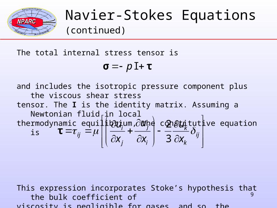
The total internal stress tensor is

and includes the isotropic pressure component plus the viscous shear stress tensor. The I is the identity matrix. Assuming a Newtonian fluid in local thermodynamic equilibrium, the constitutive equation is

This expression incorporates Stoke’s hypothesis that the bulk coefficient of viscosity is negligible for gases, and so, the second coefficient of viscosity is directly related to the coefficient of viscosity .

τσ Ip

ijk

k

i

j

j

iij x

u

x

u

x

u 3

2τ

10

Navier-Stokes Equations (continued)

The non-convective term of the flux can be separated into inviscid and viscous components in the form

The heat flux vector can be expressed as

and includes components of heat transfer due to molecular dissipation, diffusion of species, and radiation.

R

ns

iiii

jj qhU

x

Tkqq

1

VNS

INSNS DDD

I

ID

pv

p-INS

0

qv

VNS

0

D

11

Turbulence

When fluid dynamics exhibits instabilities, it is known as turbulence. Most aerospace flows of interest involve the transition of flow from a laminar condition to turbulent. Turbulence is defined as,

“…an irregular condition of flow in which the various quantities show a random variation with time and space coordinates, so that statistically distinct average values can be discerned” (Hinze, 1975).

Turbulence can be visualized as eddies (local swirling motion):• Size of eddy is turbulent length scale, but smallest still larger than molecular

length scale.

• Length scales vary considerably.

• Eddies overlap in space with large eddies carrying small eddies.

• Cascading process transfers the turbulent kinetic energy from large eddies to smaller eddies where energy is dissipated as heat energy through molecular viscosity.

• Eddies convect with flow, and so, turbulence is not local – depend on history of the eddy.

12

Reynolds-Averaging

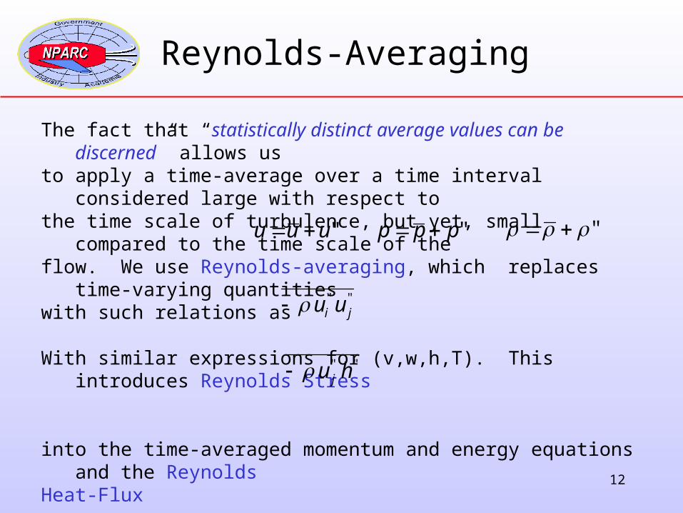
The fact that “statistically distinct average values can be discerned” allows us to apply a time-average over a time interval considered large with respect to the time scale of turbulence, but yet, small compared to the time scale of the flow. We use Reynolds-averaging, which replaces time-varying quantities with such relations as

With similar expressions for (v,w,h,T). This introduces Reynolds Stress

into the time-averaged momentum and energy equations and the Reynolds Heat-Flux

into the time-averaged energy equations.

Task of turbulence modeling is to model these terms.

"uuu "ppp "

""ji uu

"" hu j

13

Simplifications of the RANS Equations

Simplification of the full Reynolds-Averaged Navier-Stokes (RANS) equations

can be employed to allow less computational effort when certain flow physics is not to be simulated:

Thin-Layer Navier-Stokes Equations

In the case of thin boundary layers along a solid surface, one can neglect viscous terms for coordinate directions along the surface, which are generally small.

Parabolized Navier-Stokes (PNS) Equations

In addition to the thin-layer assumption, if the unsteady term is removed from the equation and flow is supersonic in the streamwise direction, then the equations become parabolic in the cross-stream coordinates and a space-marching method can be used, which reduces computational effort significantly.

Euler (Inviscid) Equations

If all viscous and heat conduction terms are removed from the RANS equations, the equations become hyperbolic in time. This assumes viscosity effects are very small (high Reynolds numbers).

14

Boundary and Initial Conditions

The Boundary Conditions for the Navier-Stokes equations will be

discussed a little later.

The type of Initial Conditions for the Navier-Stokes equations

depend on the solution method. Time-marching or iterative

methods require an initial flow field solution throughout the

domain. Space-marching methods require the flow field solution

at the starting marching surface.

15

Turbulent Modeling

Turbulence Modeling is the process of closing the Navier-Stokes equations by providing required turbulence information. Turbulence Modeling has a few fundamental classifications:

1. Models that use the Boussinesq Approximation. These are the eddy-viscosity models, which will be the focus of this presentation.

2. Models that solve directly for the Reynolds Stresses. These become complicated fast by introducing further terms requiring modeling.

3. Models not based on time-averaging. These are the Large-Eddy Simulation (LES) and Direct Numerical Simulation (DNS) methods.

16

Boussinesq Approximation

The Boussinesq Approximation essentially assumes the exchange of turbulent energy in the cascading process of eddies is analogous of that of molecular viscosity. Thus, the approximation is

which is the same form as the laminar viscous tensor. This allows us to write an effective viscosity as

Similarly the Reynolds heat-flux vector is approximated by applying the Reynolds analogy between momentum and heat transfer

with and

Thus, the objective of the turbulence model is to compute T.

k

kijTji x

uSuu

3

12""

TL

jTj x

Tkhu

""T

pTT

ck

Pr

.TL kkk

17

Turbulence Equations

There exist various turbulence models, which may be classified as

1. Algebraic Models– Cebeci-Smith– Baldwin-Lomax– PDT

2. One-Equation Models (1 pde)– Baldwin-Barth– Spalart-Allmaras (S-A)

3. Two-Equation Models (2 pdes)– SST– Chien k-epsilon

• Models mostly assume fully turbulent flow rather than accurately model transition from laminar to turbulence flow.

• One- and two-equation models attempt to model the time history of turbulence.

• Models integrate through boundary layers to the wall, but S-A and SST models allow use of a wall function.

18

Algebraic Models

Algebraic Models consist of algebraic relations to define the local eddy viscosity. The models are based on Prandtl’s Mixing Length Model that was developed through an analogy with the molecular transport of momentum.

The Cebeci-Smith Model is a two-layer model for wall-bounded flows that computes the turbulent eddy viscosity based on the distance from a wall using Prandtl’s model and empirical turbulence correlations.

The Baldwin-Lomax Model improves on the correlations of the Cebeci-Smith model and does not require evaluation of the boundary layer thickness. It is the most popular algebraic model.

The PDT Model improves on the Baldwin-Lomax model for shear layers.

Algebraic models work well for attached boundary layers under mild pressure gradients, but are not very useful when the boundary layer separates.

y

ulmixT

2

19

One-Equation Models

One-Equation Models consist of a single partial differential equation (pde) that

attempts to capture some of the history of the eddy viscosity. The Baldwin-Barth and Spalart-Allmaras turbulence models are two popular models; however, the Baldwin-Barth model has some problems and its use is not recommended.

The Spalart-Allmaras Model can be used when the boundary layer separates and has been shown to be a good, general-purpose model (at least robust to be used for a variety of applications).

20

Two-Equation Models

Two-Equation Models consist of two partial differential equations (pde) that attempts to capture some of the history of the eddy viscosity. The Menter

SST and Chien k- turbulence models are two popular models.

As the number of equations increases, the computational effort increases and one has to balance improvements in modeling with the capture of important turbulence information.

21

Chemistry Equations

The chemistry equations govern multi-species diffusion and chemical reactions

for a finite-rate fluids model. The equations consist of species continuity equations:

Where ji is the mass flux of species i defined by Fick’s first law of diffusion

The rate of formation of species i is

1

1

ns

ichem

c

c

c

Q

1

1

ns

ichem

j

j

j

D

1

1

ns

ichem

r

r

r

P

iimi cD j

dt

dXMr i

ii

22

Chemistry Equations

The net rate of formation of species i is

which is not zero for non-equilibrium flows. For the set of chemical reactions specified for the fluid, the net rate of formation can be determined from

where denotes the product. Again, note that

dt

dXMr i

ii

ss bssb

assfss

b

i

f

ii XKXKabdt

Xd

dt

Xd

dt

Xd

.i

ii M

cX

23

Magneto-Fluid Dynamic Equations

The Magneto-Fluid Dynamics Equations allow the solution of

the magnetic B and electric E fields.

24

Normalization of the Equations

The equations can be normalized (non-dimensionalized) so that non-dimensional parameters (Reynolds and Prandtl number) are explicit in the equations and values are approximately unity. Usual reference quantities are

and

with velocities non-dimensionalized by

To allow when requires

The non-dimensionalized equation of state becomes

Where at reference (freestream) conditions

This results in the relations

TTref ref

.2 TRaref

.2refrefrefref aep

.~~~~ TRp

T~a~

.1~~ Rp

.1~ R

25

Decoding the Conserved Variables

The solutions of the equations yields

for (i = 1, ns-1)

Those variables are then “decoded” to determine other flow properties:

A system of equations are iterated on temperature T to determine p, h, and T

(repeat)

1

1

1ns

iins cc i

ns

ii RcR

1

vvee t

2

1

v

v

tNS evQ ,,

ichem cQ

1 epe

h

T

T

pfi

ref

iidTchh

ns

iii hch

1

R

pT

26

Task From Here

We have defined the fluid relations and the governing

conservation equations. The task from here is to discretize

the equations to allow a computational solution and apply

numerical methods to obtain that solution.

We start with looking at a finite-volume formulation of

these equations.

Next