1 CHAPTER 9 CONVECTION IN TURBULENT CHANNEL FLOW 9.1 Introduction We will begin this subject with the criteria for fully developed velocity and temperature.

1

CHAPTER 9

CONVECTION IN TURBULENT CHANNEL FLOW 9.1 Introduction We will begin this subject with the criteria for fully developed velocity and temperature profiles. Will focus most of our attention on analyzing fully developed flows. As in Chapter 6, our analysis is limited to general boundary conditions: (i) uniform surface temperature, and (ii) uniform heat flux.

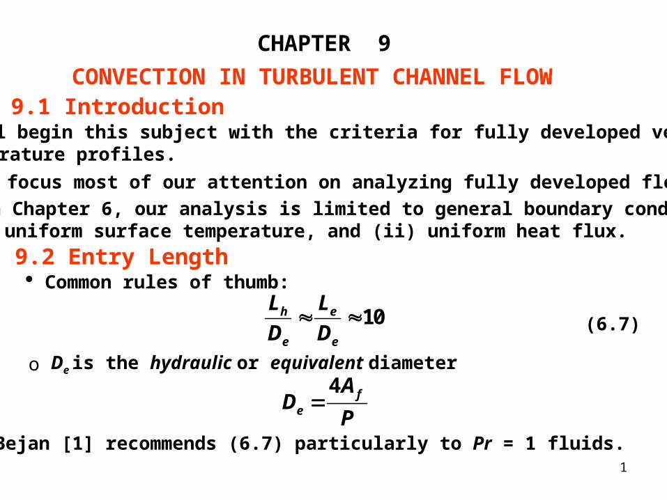
9.2 Entry Length Common rules of thumb:

10h e

e e

L L

D D (6.7)

o De is the hydraulic or equivalent diameter4 f

e

AD

P

o Bejan [1] recommends (6.7) particularly to Pr = 1 fluids.

2

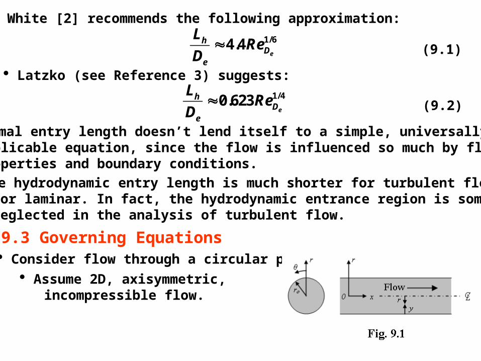
White [2] recommends the following approximation:

Latzko (see Reference 3) suggests:

Consider flow through a circular pipe.

1/64.4e

hD

e

LRe

D (9.1)

1/40.623e

hD

e

LRe

D (9.2)

Thermal entry length doesn’t lend itself to a simple, universally- applicable equation, since the flow is influenced so much by fluid properties and boundary conditions. The hydrodynamic entry length is much shorter for turbulent flow than for laminar. In fact, the hydrodynamic entrance region is sometimes neglected in the analysis of turbulent flow.

9.3 Governing Equations

Assume 2D, axisymmetric, incompressible flow.

3

9.3.1 Conservation Equations Conservation of Mass:

10r

urv

x r r

(9.3)

x-momentum equation reduces to:

1 1rr M

vu dp uu v r

x r dx r r r

(9.4)

Conservation of Energy:

1r H

T T Tu v r

x r r r r

(9.5)

9.3.2 Apparent Shear Stress and Heat Flux Similar to that of the flat plate:

appM

u

r

(9.6)

appH

p

q T

c r

(9.7)

4

9.3.3 Mean Velocity and Temperature

Calculating by evaluating the mass flow rate in the duct:

0

2or

mm u A u r dr Assuming constant density:

2 20 0

1 22

o or r

mo o

u u r dr urdrr r

(9.8)

Evaluating by integrating the total energy of the flow:

0

0

o

o

r

m r

Turdr

T

urdr

Mean Velocity

Bulk Temperature

Can be simplified by substituting the mean velocity, equation (9.8),

5

20

2 or

mm o

T Turdru r

(9.9)

Already seen that the universal velocity profile in a pipe is very similar to that of flow over a flat plate at zero or favorable pressure gradient.

9.4.1 Results from Flat Plate Flow

9.4 Universal Velocity Profile

We even adapted a pipe flow friction factor model to analyze flow over a flat plate using the momentum integral method. It is apparent, then, that the characteristics of the flow near the wall of a pipe are not influenced greatly by the curvature of the wall of the radius of the pipe. Therefore a reasonable start to modeling pipe flow is to invoke the two-layer model that we used to model flow over a flat plate:

u y (8.54) Viscous Sublayer:1

lnu y B

(8.58) Law of the Wall:

We also have continuous wall law models by Spalding (8.63) and Reichardt (8.64) that have been applied to pipe flow.

6

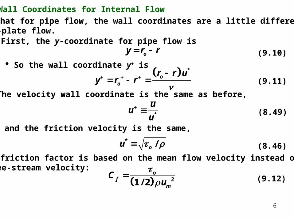
Wall Coordinates for Internal Flow Note that for pipe flow, the wall coordinates are a little different than for flat-plate flow. First, the y-coordinate for pipe flow is

oy r r (9.10) So the wall coordinate y+ is

*o

o

r r uy r r

(9.11)

The velocity wall coordinate is the same as before,

*

uu

u (8.49)

and the friction velocity is the same,

* /ou (8.46) The friction factor is based on the mean flow velocity instead of the free-stream velocity:

21 / 2o

fm

Cu

(9.12)

7

So the friction velocity can be expressed as:* / 2m fu u C

The velocity profile data for pipe flow matches that of flat plate flowo This fact allowed us to develop expressions for universal velocity profiles solely from flat plate (Cartesian) coordinates.

Would we have achieved the same results if we had started from the governing equations for pipe flow (i.e., cylindrical coordinates)?

Assume fully developed flow. x-momentum reduces to

1 1r p

r r x

(9.13)

9.4.2 Development in Cylindrical Coordinates

Rearranging and integrating, we obtain an expression for the shear stress anywhere in the flow:

( )2

r pr C

x

(9.14)

The constant C is zero, since we would expect the velocity gradient (and hence the shear stress) to zero at r = 0.

8

Evaluating (9.14) at r and ro and taking the ratio of the two gives:

This result shows that the local shear is a linear function of radial location.

( )

o o

r r

r

(9.15)

constantoM

u

r

(9.16)

Exp. data suggest that the near-wall behavior is not influenced by the outer flow, or even the curvature of the wall.

But the Couette Flow assumption meant that τ is approximately constant in the direction normal to the wall! How do we reconcile this?

o Remember that the near-wall region over which we make the Couette flow assumption covers a very small distance. o Therefore we could assume that, in that small region vary close to the wall of the pipe, the shear is nearly constant, τ = τo

o Thus the Couette assumption approximates the behavior near the pipe wall as

9

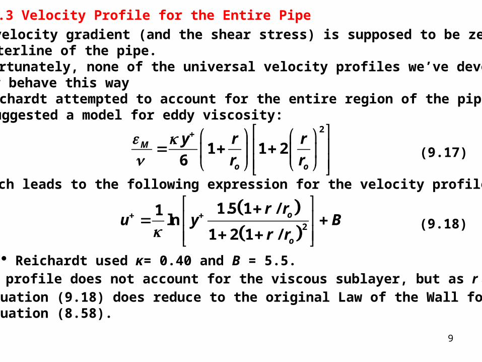
The velocity gradient (and the shear stress) is supposed to be zero at the centerline of the pipe.

2

1 1 26

M

o o

y r r

r r

(9.17)

Reichardt used κ= 0.40 and B = 5.5.

9.4.3 Velocity Profile for the Entire Pipe

Unfortunately, none of the universal velocity profiles we’ve developed so far behave this way Reichardt attempted to account for the entire region of the pipe. He suggested a model for eddy viscosity:

2

1.5 1 /1ln

1 2 1 /

o

o

r ru y B

r r

(9.18)

Which leads to the following expression for the velocity profile:

The profile does not account for the viscous sublayer, but as r →ro, equation (9.18) does reduce to the original Law of the Wall form, equation (8.58).

10

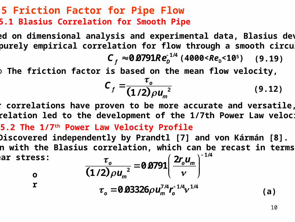
Based on dimensional analysis and experimental data, Blasius developed a purely empirical correlation for flow through a smooth circular pipe:

9.5.1 Blasius Correlation for Smooth Pipe9.5 Friction Factor for Pipe Flow

o The friction factor is based on the mean flow velocity,

Later correlations have proven to be more accurate and versatile, but this correlation led to the development of the 1/7th Power Law velocity profile.

1/40.0791f DC Re (9.19) (4000<ReD<105)

21 / 2o

fm

Cu

(9.12)

9.5.2 The 1/7th Power Law Velocity Profile Discovered independently by Prandtl [7] and von Kármán [8]. Begin with the Blasius correlation, which can be recast in terms of wall shear stress:

1/4

2

20.0791

1 / 2o o m

m

r u

u

or7/4 1/4 1/40.03326o m ou r (a)

11

Assume a power law velocity profile:

Simplifies to:

q

CL o

u y

u r

(b)

Assume that the mean velocity in the flow can be related to the centerline velocity as: constantCLu u (c) Substituting (b) and (c) for the mean velocity in (a) yields :

7/41/

1/4 1/4( )

q

o oo

yconst u r

r

7/4 ( 7/4 ) (7/4 1/4) 1/4( ) q qo oconst u y r (d)

Both Prandtl and von Kármán argued that the wall shear stress is not a function of the size of the pipe. Then the exponent on ro should be equal to zero. Setting the exponent to zero, the value of q must be equal to 1/7, leading to the classic 1/7th power law velocity profile,

12

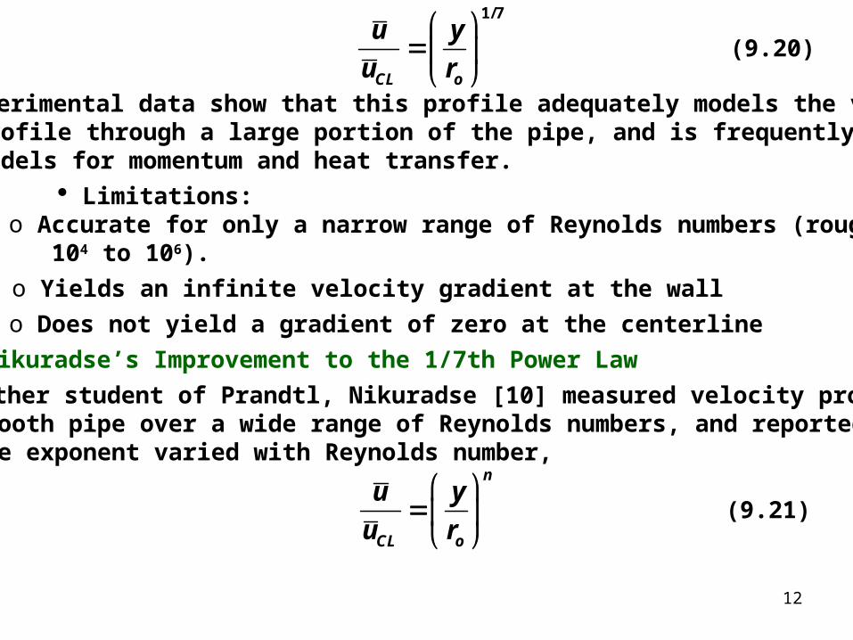
o Accurate for only a narrow range of Reynolds numbers (roughly, 104 to 106).

Experimental data show that this profile adequately models the velocity profile through a large portion of the pipe, and is frequently used in models for momentum and heat transfer.

1/7

CL o

u y

u r

(9.20)

Limitations:

Another student of Prandtl, Nikuradse [10] measured velocity profiles in smooth pipe over a wide range of Reynolds numbers, and reported that the exponent varied with Reynolds number,

o Yields an infinite velocity gradient at the wall

o Does not yield a gradient of zero at the centerline

Nikuradse’s Improvement to the 1/7th Power Law

n

CL o

u y

u r

(9.21)

13

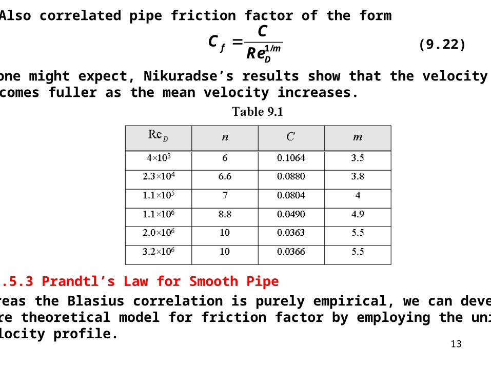
Also correlated pipe friction factor of the form

1/f mD

CC

Re (9.22)

As one might expect, Nikuradse’s results show that the velocity profile becomes fuller as the mean velocity increases.

9.5.3 Prandtl’s Law for Smooth Pipe Whereas the Blasius correlation is purely empirical, we can develop a more theoretical model for friction factor by employing the universal velocity profile.

14

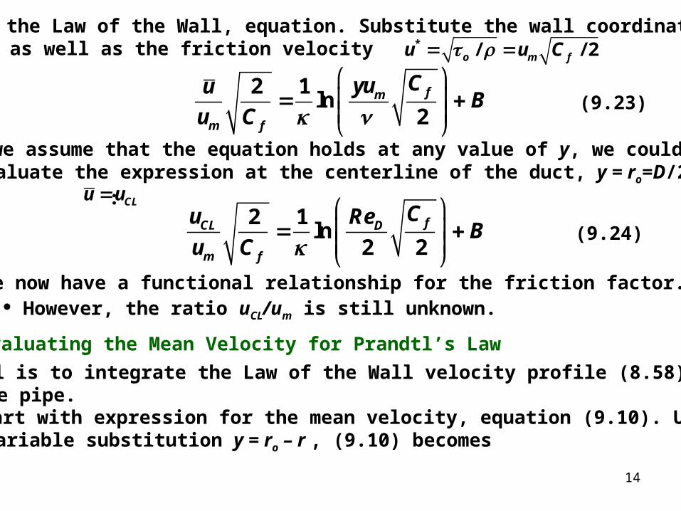
Begin with the Law of the Wall, equation. Substitute the wall coordinates u+ and y+, as well as the friction velocity :* / / 2o m fu u C

We now have a functional relationship for the friction factor.

2 1ln

2fm

m f

CyuuB

u C

(9.23)

If we assume that the equation holds at any value of y, we could evaluate the expression at the centerline of the duct, y = ro=D/2, where :CLu u

2 1ln

2 2fCL D

m f

Cu ReB

u C

(9.24)

However, the ratio uCL/um is still unknown.

Evaluating the Mean Velocity for Prandtl’s Law Goal is to integrate the Law of the Wall velocity profile (8.58) across the pipe. Start with expression for the mean velocity, equation (9.10). Using the variable substitution y = ro – r , (9.10) becomes

15

2 20 0

1 2(2 ) ( )

o or r

m oo o

u u r dr u r y dyr r

(9.25)

Then, substitute the Law of the Wall for .u

** 1 3

ln2

om

r uu u B

(9.26)

Performing the integration, it can be shown that the mean velocity becomes

We can use the above expression directly to find an expression for Cf. Rearranging, and substituting the values κ= 0.41 and B = 5.0 gives

1 3ln

2 2 2 2f fD

m m

C Cu u B

Re(9.27)

Or, making substitutions again for u*

Warning: the term we were trying to evaluate, um, cancels out of the expression! However, uCL doesn’t not appear either.

12.44ln / 2 0.349

/ 2D f

f

CC

Re

16

12.46ln / 2 / 2 0.29 ( 4000)

/ 2f D f D

f

C C ReC

(9.28)

This development ignores the presence of a viscous sublayer or a wake region.

Note that, despite the empiricism of using a curve fit to obtain the constants in (9.28), using a more theoretical basis to develop the function has given the result a wider range of applicability than Blasius’s correlation. Equation (9.28) must be solved iteratively for Cf. A simpler, empirical relation that closely matches Prandtl’s is:

Empirically, a better fit to experimental data is

This is called Prandtl’s universal law of friction for smooth pipes. o Sometimes referred to as the Kármán-Nikuradse equation.

1/5 4 60.023 (3 10 < 10 )2

fD D

CRe Re (9.29)

This correlation is also suitable for non-circular ducts, with the Reynolds number calculated using the hydraulic diameter.

17

From our discussion of turbulent flow over a rough flat plate, we saw that roughness shifts the universal velocity profile downward.

ΔB is the shift in the curve, which increases with wall roughness k+

9.5.4 Effect of Surface Roughness

We could write the velocity profile in the logarithmic layer as:1

lnu y B B

The behavior of the velocity profile also depends on the geometrygeometry of the roughness, like rivets to random structures like sandblasted metal.

The following model is based on equivalent sand grain roughness [2],1/2

101/2 1/2

12.0 log 0.8

1 0.1( / )D

D

f

f k D f

Re

Re(9.30)

where it is common to use the Darcy friction factor,

4 ff C (9.31)

Two Important Points on Surface Roughness:

1. If the relative roughness k/D is low enough, it doesn’t have much of an effect on the equation.

18

o Scaling shows that roughness is not important if / 10Dk D Re

Developed for commercial pipes,

101/2 1/2

1 / 2.512.0 log

3.7 D

k D

f f

Re(9.32)

Colebrook-White Equation

2. On the other hand, if , the roughness term dominates in the denominator, and the Reynolds number cancels; in other words, the friction factor is no longer dependent on the ReD.

/ 1000Dk D Re

This function is what appears in the classic Moody Chart

19

Moody Chart:

20

Strictly speaking, an analogy cannot be made in pipe flow for the case of a constant surface temperature. But resulting models approximately hold for this case as well.

9.6 Momentum-Heat Transfer Analogies

x-momentum equation (9.4) becomes, for hydrodynamically fully developed flow,

Are the left-hand sides analogous?

Development is applied to the case of a constant heat flux boundary condition.

Development

1 1M

dp ur

dx r r r

(9.33a)

1H

T Tu r

x r r r

(9.33b)

Energy equation reduces to,

21

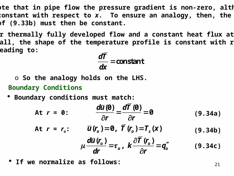
o Note that in pipe flow the pressure gradient is non-zero, although constant with respect to x. To ensure an analogy, then, the left side of (9.33b) must then be constant.

constantdT

dx

Boundary conditions must match:

o For thermally fully developed flow and a constant heat flux at the wall, the shape of the temperature profile is constant with respect to x, leading to:

o So the analogy holds on the LHS.

Boundary Conditions

(0) (0)0

du dT

r r

(9.34a) At r = 0:

( ) 0, ( ) ( )o o su r T r T x (9.34b) At r = ro:

( ) ( ), o o

o o

du r T rk q

dr r

(9.34c)

If we normalize as follows:

22

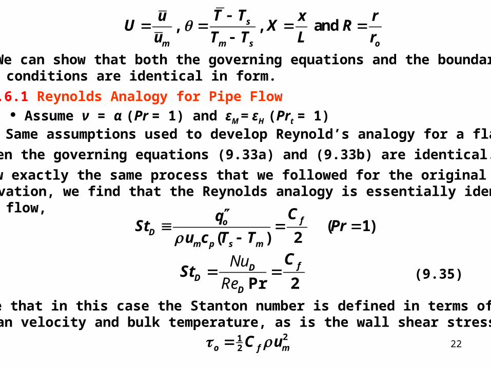
We can show that both the governing equations and the boundary conditions are identical in form.

o Same assumptions used to develop Reynold’s analogy for a flat plate

Pr 2fD

DD

CSt

Nu

Re(9.35)

, , and s

m m s o

T Tu x rU X R

u T T L r

9.6.1 Reynolds Analogy for Pipe Flow Assume ν = α (Pr = 1) and εM = εH (Prt = 1)

Then the governing equations (9.33a) and (9.33b) are identical. Follow exactly the same process that we followed for the original derivation, we find that the Reynolds analogy is essentially identical for pipe flow,

( 1)( ) 2

foD

m p s m

CqSt Pr

u c T T

Note that in this case the Stanton number is defined in terms of the mean velocity and bulk temperature, as is the wall shear stress:

212o f mC u

23

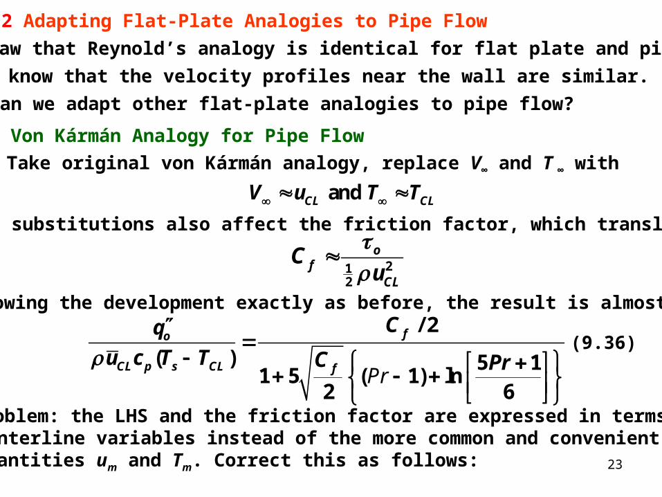
/ 2

( ) 5 11 5 ( 1) ln

2 6

fo

CL p s CL f

Cq

u c T T C Pr

Pr

(9.36)

9.6.2 Adapting Flat-Plate Analogies to Pipe Flow We saw that Reynold’s analogy is identical for flat plate and pipe flows.

Take original von Kármán analogy, replace V∞ and T ∞ with

These substitutions also affect the friction factor, which translates to:

and CL CLV u T T

Problem: the LHS and the friction factor are expressed in terms of centerline variables instead of the more common and convenient mean quantities um and Tm. Correct this as follows:

We know that the velocity profiles near the wall are similar. Can we adapt other flat-plate analogies to pipe flow?

Von Kármán Analogy for Pipe Flow

212

of

CL

Cu

Following the development exactly as before, the result is almost identical:

24

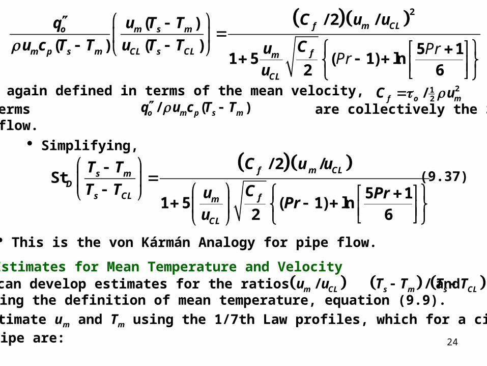
2/ 2 /( )

( ) ( ) 5 11 5 ( 1) ln

2 6

f m CLo m s m

m p s m CL s CL fm

CL

C u uq u T T

u c T T u T T Cu

u

PrPr

This is the von Kármán Analogy for pipe flow.

Simplifying,

Now, Cf is again defined in terms of the mean velocity, and the terms are collectively the Stanton number for pipe flow.

212/f o mC u

/ ( )o m p s mq u c T T

/ 2 /St

5 11 5 ( 1) ln

2 6

f m CLs mD

s CL fm

CL

C u uT T

T T Cu PrPr

u

(9.37)

Estimates for Mean Temperature and Velocity We can develop estimates for the ratios and using the definition of mean temperature, equation (9.9).

/m CLu u /s m s CLT T T T

Estimate um and Tm using the 1/7th Law profiles, which for a circular pipe are:

25

Substituting these models into (9.8) and (9.9), we can show that:

and, similar to (8.111) for a flat plate,

1/7

CL o

u y

u r

(9.20)

A simple correlation for turbulent flow in a duct is based on the Colburn analogy. Beginning with the analogy, equation (8.96), and using equation (9.27) for the friction factor, we obtain

1/7

s

CL s o

T T y

T T r

(9.38)

0.817m

CL

u

u (9.39)

0.833m s

CL s

T T

T T

(9.40)

9.6.3 Other Analogy-Based Correlations

26

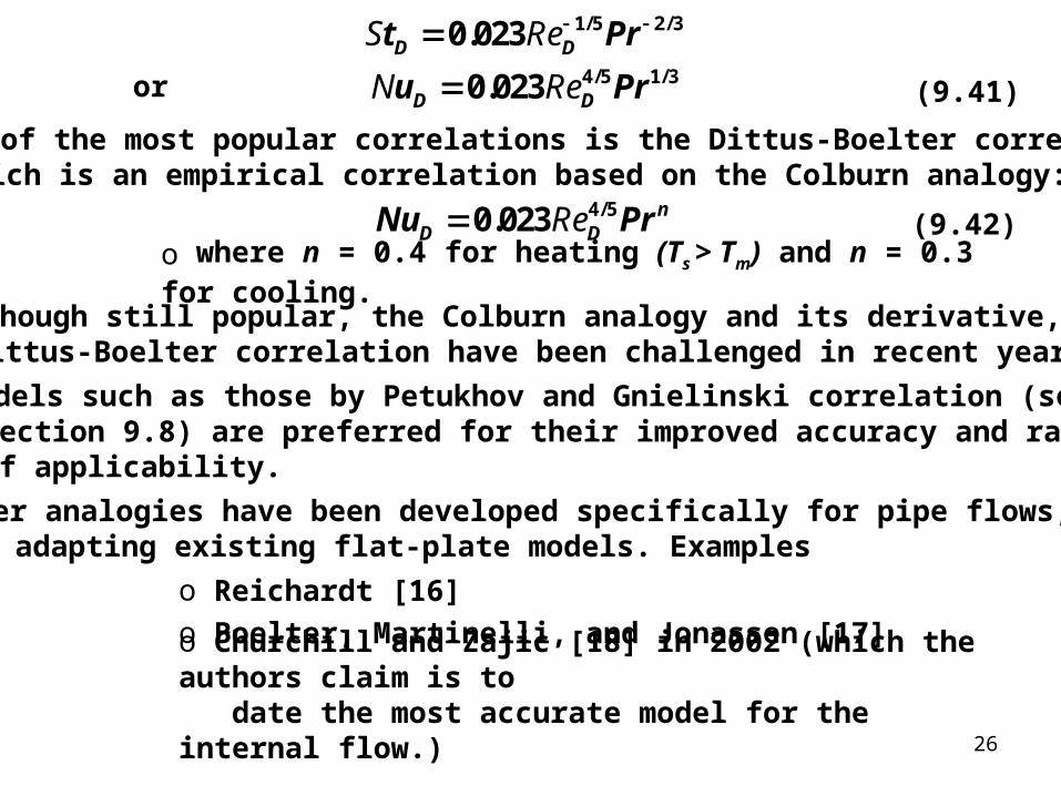
One of the most popular correlations is the Dittus-Boelter correlation, which is an empirical correlation based on the Colburn analogy:

1/5 2/30.023D Dt Pr S Re

o where n = 0.4 for heating (Ts > Tm) and n = 0.3 for cooling.

or 4/5 1/30.023D Du PrN Re (9.41)

4/50.023 nD DNu Pr Re (9.42)

Although still popular, the Colburn analogy and its derivative, the Dittus-Boelter correlation have been challenged in recent years. Models such as those by Petukhov and Gnielinski correlation (see Section 9.8) are preferred for their improved accuracy and range of applicability. Other analogies have been developed specifically for pipe flows, instead of adapting existing flat-plate models. Examples

o Reichardt [16] o Boelter, Martinelli, and Jonassen [17]

o Churchill and Zajic [18] in 2002 (which the authors claim is to date the most accurate model for the internal flow.)

27

Begin again with the definition of the Nusselt number, which for flow in a duct can be expressed as

9.7 Algebraic Method Using Universal Temperature Profile As we did for flow over a flat plate, we can use the universal temperature and velocity profiles to estimate the heat transfer in a circular duct.

( )o

Ds m

q DhDu

k T T k

N (9.43)

* / 2( ) ( )

p m fpm s m s m

o o

c u Cc uT T T T T

q q

(9.44)

To later invoke the universal temperature profile, we use the definition of T+, equation 8.102, to define the mean temperature as

Recall that for duct flow, the friction velocity u* is defined in terms of the mean velocity. Substituting this expression into (9.43) for and invoking the definitions of the Reynolds and Prandtl numbers,

oq

/ 2D f

Dm

Pr C

T Re

Nu (9.45)

28

Several ways to proceed with the analysis. One approach is to evaluate Tm

+ using a dimensionless version of the mean temperature expression (9.33):

20

2( )

or

m om o

T T u r y dyu r

(9.46)

( )

( ) ( )o s CL

Ds m s CL

q D T T

T T k T T

Nu

A simpler, second approach can be taken. First, we rewrite the original Nusselt number relation (9.43) as follows,

Then, substitute the definition of T+ for the centerline temperature in the denominator, we obtain

/ 2 ( )

( )D f s CL

DCL s m

Pr C T Tu

T T T

ReN (9.47)

Theoretically, can simply substitute appropriate universal temperature and velocity profiles into the above and integrate. Practically, this requires numerical integration.

where TCL is the centerline temperature.

29

We can now use the universal temperature profile, equation (8.118), to evaluate TCL

+:2/3ln 13 7t

CL CL

PrT y Pr

(9.48)

Substituting these into the Nusselt number relation,

*

2CL CLCL

m f

u uu

u u C (9.51)

Now, just like in our analysis for flat plate flow, we can substitute the Law of the Wall velocity profile (8.59) for ln yCL

+:

1lnCL CLu y B

(9.49)

2/3

/ 2 ( )

( )( ) 13 7

D f s CLD

s mt CL

Pr C T TNu

T TPr u B Pr

Re(9.50)

We need expressions for and . For the centerline velocity, we can use the definition of u+ for pipe flow:

CLu ( ) / ( )s CL s mT T T T

30

It appears that, if we are to complete the analysis, we will need to evaluate the mean velocity and temperature after all. To avoid the complexity of the logarithmic velocity and temperature profiles, we could estimate these quantities using the much simpler 1/7th Law profiles, which we saw in the last section yields

2/3

/ 2

0.92 10.8 0.89 / 2f

D

f

CSt

Pr C

(9.52)

Finally, using the definition of Stanton number, , selecting Prt = 0.9 and B = 5.0, we can rearrange (9.50) obtain

/ ( )D D DSt Nu Re Pr

0.817m

CL

u

u (9.39)

0.833m s

CL s

T T

T T

(9.40)

Under what conditions is this equation applicable? The ultimate test would be to compare the expression to experimental data. However, since we invoked the 1/7th power law, which is valid around 1×105, it might be reasonable as a first approximation to limit this model to ReD < 1×105.

31

Petukhov followed a more rigorous theoretical development, invoked Reichardt’s model for eddy diffusivity and velocity profile (9.15, 9.16):

9.8 Other Correlations for Smooth Pipes

4 62/3

/ 2 0.5 2000,

10 5 101.07 12.7 1 / 2f

DDf

C PrSt

RePr C

(9.53)

2(2.236ln 4.639)2

fD

CRe (9.54)

Compares well to experimental data over a wide range of Prandtl and Reynolds numbers.

Petukhov’s Model

Petukhov used the following model for friction factor, which he also developed:

Note the similarity between Petukhov’s relation (9.53) and the algebraic result, equation (9.52). It seems as if we have captured the essential functionality even in our modest approach.

Gnielinski’s Model Gnielinski modified Petukhov’s model slightly, extending the model to include lower Reynolds numbers:

32

3 62/3

( 1000) / 2 0.5 2000,

3 10 5 101 12.7 1 / 2D f

DDf

Re PrC Pru

RePr C

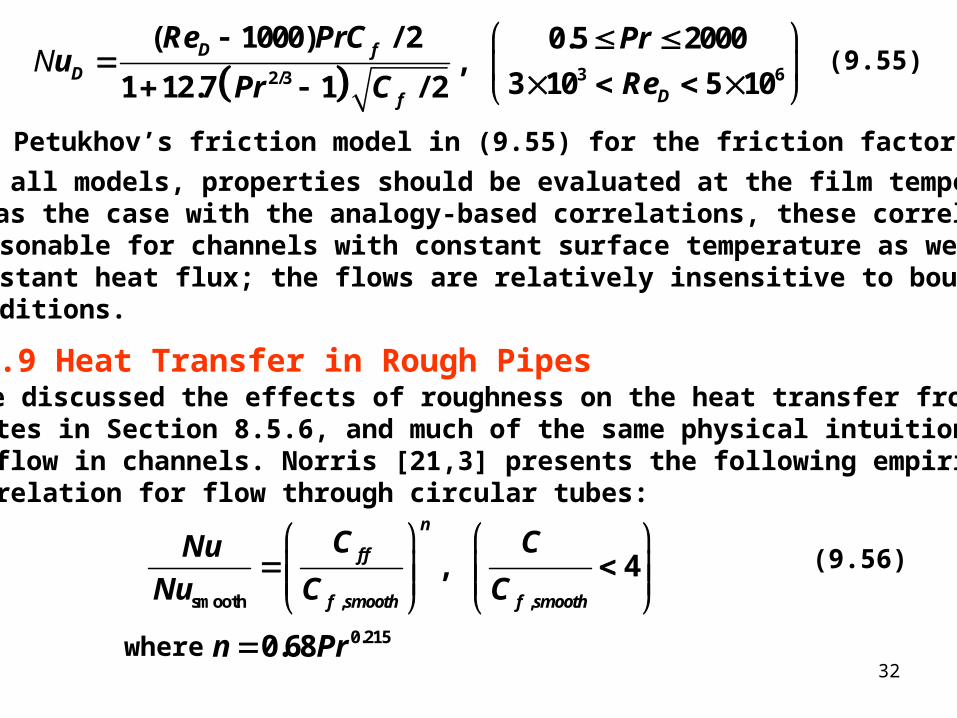
N (9.55)

Use Petukhov’s friction model in (9.55) for the friction factor.

We’ve discussed the effects of roughness on the heat transfer from flat plates in Section 8.5.6, and much of the same physical intuition applies to flow in channels. Norris [21,3] presents the following empirical correlation for flow through circular tubes:

For all models, properties should be evaluated at the film temperature. As was the case with the analogy-based correlations, these correlations are reasonable for channels with constant surface temperature as well as constant heat flux; the flows are relatively insensitive to boundary conditions.

9.9 Heat Transfer in Rough Pipes

smooth , ,

, 4

n

f f

f smooth f smooth

C CNu

Nu C C

(9.56)

where 0.2150.68n Pr

33

A correlation like Colebrook’s (9.30) could be used to determine the rough-pipe friction factor. The behavior of this relation reflects what we expect physically.

o The Prandtl number influences the effect of roughness, and for very low-Pr fluids the roughness plays little role in the heat transfer. o Regardless of Prandtl number, the influence of roughness size is limited: Norris reports that the effect of increasing roughness vanishes beyond , and so the equation reaches a maximum.

,( / ) 4f f smoothC C

Although roughness enhances heat transfer, it also increases the friction. Neither the friction nor the heat transfer increase indefinitely with roughness size – both reach a limiting value.