1 Chapter 5 Two-Way Tables Associations Between Categorical Variables.

1

Chapter 5

Two-Way Tables Associations Between Categorical Variables

2

• Quantitative variables correlation [Ch 3] & regression [Ch 4]

• categorical variables two-way tables of frequency counts [Ch 5]

Associations between variables

3

Two-Way Table of CountsR-by-C tables

Variables

AGE variable = column variable (3 levels)

EDUCATION variable = row variable (4 levels)

This is a 4-by-3 table

4

Marginal Distributions

Variables

Row variablemarginal totals

37,786 81,435 56,008

27,85858,07744,46544,828

Column variablemarginal distribution

5

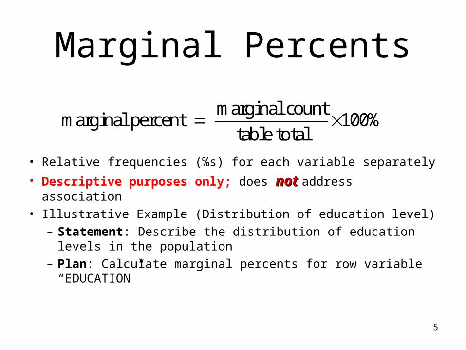
Marginal Percents

• Relative frequencies (%s) for each variable separately

• Descriptive purposes only; does not not address association

• Illustrative Example (Distribution of education level)

– Statement: Describe the distribution of education levels in the population

– Plan: Calculate marginal percents for row variable “EDUCATION”

marginal countmarginal percent 100%

table total

6

Marginal Percents Example

% not completing HS = 27,859 / 175,230 × 100% = 15.9%

% completing HS = 58,077 / 175,230 × 100% = 33.1%

% with 1-3 yrs college = 44,465 / 175,230 × 100% = 25.4%

% with 4+ yrs college = 44,828 / 175,230 × 100% = 25.6%

Step 3: “Solve”

Rowtotals

Tabletotal

7

Marginal Percents (Example)

• 16% did not complete high school

• 33% completed high school

• 25% completed 1 to 3 years of college

• 26% completed 4+ years of college

Step 4: “Conclude”

Merely descriptive statements

8

Association

• If the row variable is the explanatory variable → compare conditional row proportions

• If the column variable is the explanatory variable → compare conditional column proportions

cell countconditional row proportion

row total

cell countconditional column proportion

column total

Use conditional proportions to determine associations

9

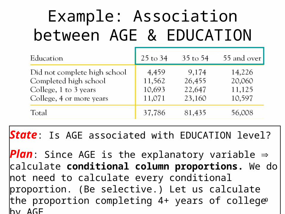
Example: Association between AGE & EDUCATION

State: Is AGE associated with EDUCATION level?

Plan: Since AGE is the explanatory variable calculate conditional column proportions. We do not need to calculate every conditional proportion. (Be selective.) Let us calculate the proportion completing 4+ years of college by AGE

10

Example: “Solve” & “Conclude”

p̂ 25-34

11,071 = .2930 = 29%

37,786

55ˆ =p 10,597

.1892 = 19%56,008

35 54p̂ 23,160

= .2843 = 28%81,435

ˆLet p represent proportion completing 4+ years of college

Conclude: As age goes up, % completing college goes down Negative association between age and college completion

11

• No association: conditional percents nearly equal at all levels of the explanatory variable

• Positive association: as explanatory variable rises conditional percentages increase

• Negative associations: as explanatory variable rises conditional percentages go down

Direction of association

12

State: Is ACCEPTANCE into UC Berkeley graduate school (response variable) associated with GENDER (explanatory variable)?

Example: Gender bias?

Accepted Not accept. TotalMale 198 162 360Female 88 112 200Total 286 274 560

Plan: Since GENDER is the explanatory variable calculate row percents (acceptance “rates” by gender); compare % accepted by GENDER

13

Example: “Gender bias?”

Accepted Not accept TotalMale 198 162 360Female 88 112 200Total 286 274 560

Conclude: positive association between “maleness” and acceptance

Step 3: Solve

14

Simpson’s Paradox

• Lurking variable MAJOR applied to– Business school major (240 applicants) – Art school major (320 applicants)

• State: Does lurking variable explain association between maleness and acceptance?

• Plan: Subdivide (“stratify”) data into subgroups according to lurking variable MAJOR then calculate acceptance rates by gender within subgroups

Simpson’s Paradox ≡ lurking variable reverses direction of the association

15

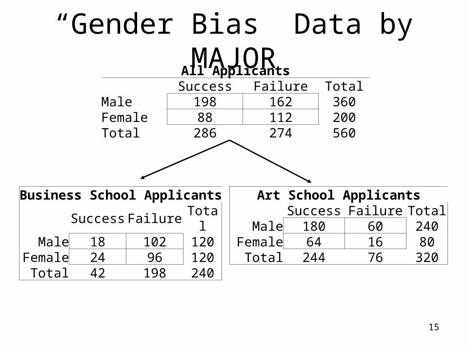
“Gender Bias” Data by MAJOR

Business School ApplicantsSuccess Failure Total

Male 18 102 120Female 24 96 120

Total 42 198 240

All ApplicantsSuccess Failure Total

Male 198 162 360Female 88 112 200Total 286 274 560

Art School ApplicantsSuccess Failure Total

Male 180 60 240Female 64 16 80

Total 244 76 320

16

Business School ApplicantsSuccess Failure Total

Male 18 102 120

Female 24 96 120

Total 42 198 240

Conclude: Negative association with maleness

0.15 18

proportion accepted, males 120

240.20 proportion accepted, females

120

Conclude: Negative association with maleness

0.15 18

proportion accepted, males 120

240.20 proportion accepted, females

120

17

Art School Applicants

Success Failure Total

Male 180 60 240

Female 64 16 80

Total 244 76 320

Conclude: Negative association with maleness

0.75240

180

proportion accepted, males

640.80 proportion accepted, females

80

18

• Overall: higher acceptance rate for men

• Within Business school: higher acceptance rate for women

• Within Art school: higher acceptance rate for women

• Therefore, the lurking variable (MAJOR) reversed the direction of the association (Simpson’s Paradox)

• Acceptance to grad school at UC Berkeley favored women after “controlling for” MAJOR

Gender Bias Example Conclusion

19

HIV vaccine boostHIV vaccine boost (Exercise 5.6)

State: Do data support that vaccine delivered by EP results in a higher proportion responding?Plan = ?Solution = ?Conclusion = ?

Kidney StonesKidney Stones (Exercise 5.7)

Small Stones

Open Surgery

Percutaneous

Success 81 234

Failure 6 36

Large Stones

Open Surgery

Percutaneous

Success 192 55

Failure 71 25

(a) Find % of kidney stones, combining the data for small and large stones, that were successfully removed for each of the two procedures. Which procedure had the higher overall success rate?(b) What % of all small kidney stones were successfully removed? What % of all large kidney stones…? Which type of kidney stone is easier to treat?

22

Helicopter EvacuationHelicopter Evacuation Lurking Variable /SimpsonSimpson’’s Paradoxs Paradox

X

Helicopter or RoadY

Survived or Died

ZAccident Severity