1 Chapter 5 Local Search. 2 Outline Local search basics General local search algorithm Hill-climbing Tabu search Simulated Annealing WSAT Conclusions.

1

Chapter 5

Local Search

2

Outline

Local search basics General local search algorithm Hill-climbing Tabu search Simulated Annealing WSAT Conclusions

3

What is local search? Local search is a family of general-purpose

techniques for search and optimization problems. The application of Local search algorithms to

optimization problems start early 1960s. Since then the interests in this subject has grown in the fields of Operations Research, CS and AI.

Local Search algorithms are non-exhaustive in the sense that they do not guarantee to find an optimal solution, but they search non-systematicaly until a specific stop criterion is satisfied.

These techniques are very appealing because of their effectiveness and their widespread applicability

4

LOCAL SEARCH BASICS Definition 1.1 (Combinatorical Optimization

Problems) We define an instance of a combina-torial optimization problem as a triple <S, F, f>, where S is a finite set of solutions, F S is a set of feasible solutions and f: S denotes an objective function that assesses the quality of each solution in S.

The issue is to find a global optimum ,i.e., an element x* F such that f(x*) f(x) for all x F.

In these settings, the set F is called feasible set and its elements feasible solutions. The relation x F is called constraint.

Example: the min-Graph-Coloring problem

5

Definition 1.2 (Search Problems) Given a pair <S,F> where S is the set of solutions and F S is the set of feasible solutions, a search problem consists of finding a feasible solution, i.e. an element x F.

There are three main entities in Local Search algorithms: (1) the search space, (2) the neighborhood relation and (3) the cost function.

Example: the k-Graph-Coloring problem

Definition 1.3 (Search space) Given a combinatorial optimization problem , we associate to each instance of it a search space S, with the following properties: 1) Each element s S represent an element x S. 2) At least one optimal element of F is represented in S

In general, the search space S and the set of solutions S of a problem are equal, but there are a few cases in which these entities differ.

6

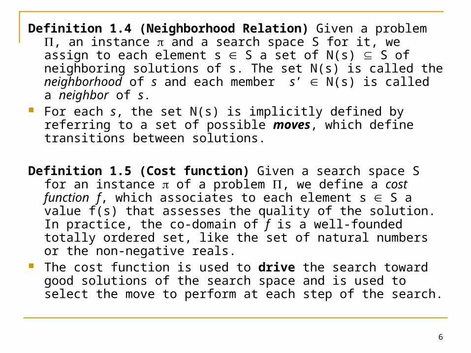
Definition 1.4 (Neighborhood Relation) Given a problem , an instance and a search space S for it, we assign to each element s S a set of N(s) S of neighboring solutions of s. The set N(s) is called the neighborhood of s and each member s’ N(s) is called a neighbor of s.

For each s, the set N(s) is implicitly defined by referring to a set of possible moves, which define transitions between solutions.

Definition 1.5 (Cost function) Given a search space S for an instance of a problem , we define a cost function f, which associates to each element s S a value f(s) that assesses the quality of the solution. In practice, the co-domain of f is a well-founded totally ordered set, like the set of natural numbers or the non-negative reals.

The cost function is used to drive the search toward good solutions of the search space and is used to select the move to perform at each step of the search.

7

General Local Search Algorithm

A local search algorithm starts from an initial solution s0 S, and iterates exploring the search space, using the moves associated with the neighborhood definition. At each step it makes a transition between one solution s to one of its neighbors s’. When the algorithm makes the transition from s to s’, we say that the corresponding move m has been accepted, and we write that s’ is equal to sm.

The selection of moves is based on the values of the cost function.

As for the initial solution s0, for some techniques its construction is part of the algorithm. For other methods, s0 can be freely constructed by some algorithm or generated randomly.

The stop criterion is part of the specific technique, and it is based either on specific qualities of the solution reached or on a maximum number of iterations.

8

procedure LocalSearch(MaxCost, MaxMoves)begin

let s = {(vi, dij)| dij Di for all vi V} be the initial solution while f(s) > MaxCost and TotalMoves < MaxMoves do begin M’ GenerateLocalMoves(s, TotalMoves) if M’ then MakeLocalMoves(s, M’, TotalMoves) endend

M the set of all local moves from the solution s. M’ M. The GenerateLocalMoves procedure returns the set of all best

moves M’ in the neighborhood of s. The GenerateLocalMoves and MakeLocalMoves functions will be

defined with details in specific local search methods.

9

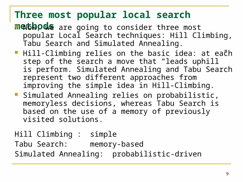
Three most popular local search methods Now, we are going to consider three most popular Local

Search techniques: Hill Climbing, Tabu Search and Simulated Annealing.

Hill-Climbing relies on the basic idea: at each step of the search a move that “leads uphill” is perform. Simulated Annealing and Tabu Search represent two different approaches from improving the simple idea in Hill-Climbing.

Simulated Annealing relies on probabilistic, memoryless decisions, whereas Tabu Search is based on the use of a memory of previously visited solutions.

Hill Climbing : simpleTabu Search: memory-basedSimulated Annealing: probabilistic-driven

10

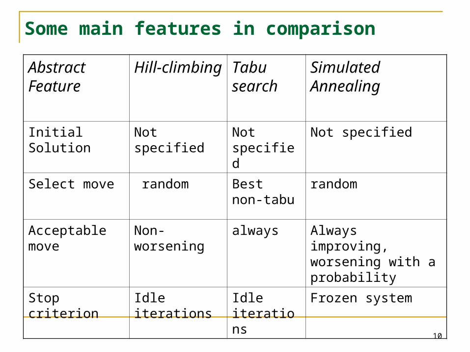
Some main features in comparison

Abstract Feature

Hill-climbing Tabu search

Simulated Annealing

Initial Solution Not specified Not specified

Not specified

Select move random Best non-tabu

random

Acceptable move

Non-worsening always Always improving, worsening with a probability

Stop criterion Idle iterations Idle iterations

Frozen system

11

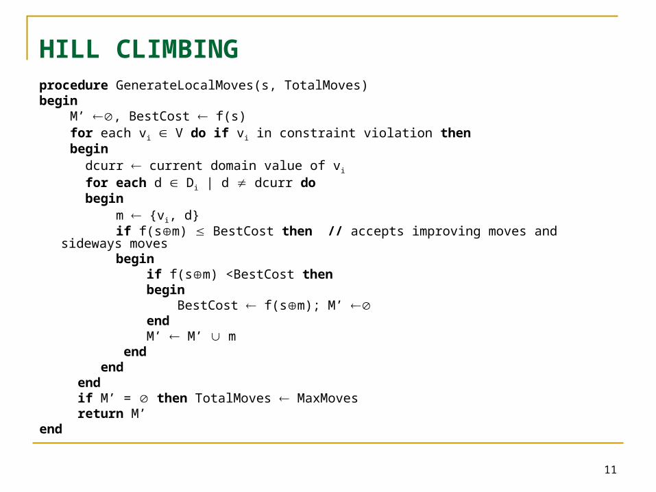
HILL CLIMBING procedure GenerateLocalMoves(s, TotalMoves)begin M’ , BestCost f(s) for each vi V do if vi in constraint violation then begin dcurr current domain value of vi

for each d Di | d dcurr do begin m {vi, d} if f(sm) BestCost then // accepts improving moves and sideways moves begin if f(sm) <BestCost then begin BestCost f(sm); M’ end M’ M’ m end end end if M’ = then TotalMoves MaxMoves return M’end

12

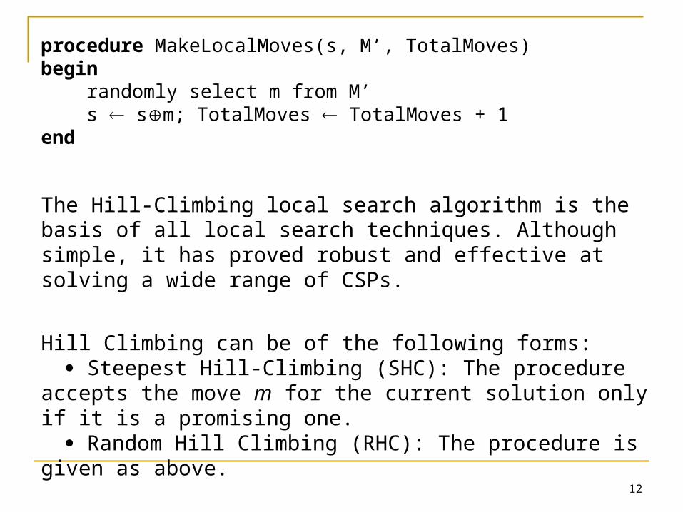
procedure MakeLocalMoves(s, M’, TotalMoves)begin randomly select m from M’ s sm; TotalMoves TotalMoves + 1end

The Hill-Climbing local search algorithm is the basis of all local search techniques. Although simple, it has proved robust and effective at solving a wide range of CSPs.

Hill Climbing can be of the following forms: Steepest Hill-Climbing (SHC): The procedure accepts the move m for the current solution only if it is a promising one. Random Hill Climbing (RHC): The procedure is given as above.

13

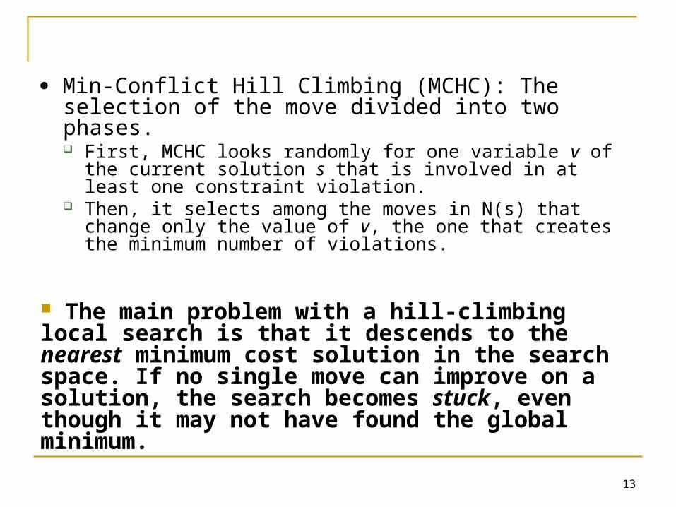
Min-Conflict Hill Climbing (MCHC): The selection of the move divided into two phases. First, MCHC looks randomly for one variable v of the

current solution s that is involved in at least one constraint violation.

Then, it selects among the moves in N(s) that change only the value of v, the one that creates the minimum number of violations.

The main problem with a hill-climbing local search is that it descends to the nearest minimum cost solution in the search space. If no single move can improve on a solution, the search becomes stuck, even though it may not have found the global minimum.

14

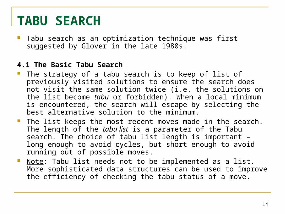
TABU SEARCH Tabu search as an optimization technique was first suggested by

Glover in the late 1980s.

4.1 The Basic Tabu Search The strategy of a tabu search is to keep of list of previously visited

solutions to ensure the search does not visit the same solution twice (i.e. the solutions on the list become tabu or forbidden). When a local minimum is encountered, the search will escape by selecting the best alternative solution to the minimum.

The list keeps the most recent moves made in the search. The length of the tabu list is a parameter of the Tabu search. The choice of tabu list length is important – long enough to avoid cycles, but short enough to avoid running out of possible moves.

Note: Tabu list needs not to be implemented as a list. More sophisticated data structures can be used to improve the efficiency of checking the tabu status of a move.

15

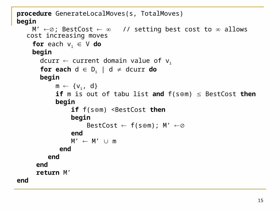
procedure GenerateLocalMoves(s, TotalMoves)begin M’ ; BestCost // setting best cost to allows cost increasing moves for each vi V do begin dcurr current domain value of vi

for each d Di | d dcurr do begin m {vi, d} if m is out of tabu list and f(sm) BestCost then begin if f(sm) <BestCost then begin BestCost f(sm); M’ end M’ M’ m end end end return M’end

16

The basic Tabu search (cont.)procedure MakeLocalMoves(s, M’, TotalMoves)begin randomly select m from M’ s sm; TotalMoves TotalMoves + 1; update tabu listend

One of the key issues of Tabu Search is the tabu tenure mechanism, i.e. the way in which we fix the number of iterations that a move should be considered as tabu.

17

Some Improvements on Tabu search A number of more complex tabu search techniques have been

developed:

Aspiration Level Conditions Notice that moves, not solutions, are asserted to be tabu.

Therefore, a move can be tabu, even if, when applied to the current solution s, it leads to an unvisited solution. In other words, the basic Tabu Search scheme avoids visiting not only previous solutions, but also solutions that share features with the already visited ones.

This mechanism prevents cycling, but in its simple form it can skip good solutions. For this reason, there is a mechanism called aspiration criterion that overrides the tabu status of a move: if in a solution s a move m give a large improvement of the cost function, the solution sm is accepted as the new current one regardless of its tabu status.

18

This mechanism makes use of an aspiration function A. For each value t of the cost function, A computes the cost value that the algorithm aspires to reach starting from t. Given a current solution s, the cost function f, and the best neighbor solution s’, if f(s’) A(f(s)), then s’ becomes the new current solution, even if the move m that leads to s’ has a tabu status.

In short, the main control parameters of the basic tabu Search are: the length of the tabu list the aspiration function A the definition of the set of neighbor solutions tested at each

iteration.

19

Reactive Search

Battiti, 1996 extended the idea of a fixed length tabu list, by proposing the length of the tabu list should vary according to the current state of the search. The search should concentrate in promising areas, but also be

able to diversify once an area no longer appears promising. Hertz et al., 1995, proposed adjusting the cost function

so that solution with similar characteristics are either penalised or rewarded depending on whether concentration (intensification) or diversification is desired.

Both schemes represent a reactive search, that changes behavior through feedback about the current state of the search.

20

Reactive search (cont.)

Reactive Tabu Search by Battiti operates on the principle: “the more a search attempts to re-visit the same solution, the more diversification is required. The fewer repetitions there are, the more concentrated a search has to be in order not to miss a promising solution.”

In Battiti’s method, diversification is controlled by allowing the length of the tabu list to grow as more repetitions are encountered, and to shrink as the number of repetitions decrease.

21

SIMULATED ANNEALING Simulated Annealing (SA) as an optimization technique was first

suggested by S. Kirkpatrick et al. in 1983. It is a variant of local search which allows uphill moves to be accepted in a controlled manner.

This technique simulates the cooling of material in a heat bath. This is a process known as annealing. If you heat a solid past melting point and then cool it, the structural properties of the solid depends on the rate of cooling.

If the liquid is cooled slowly enough, large crystals will be formed. However, if the liquid is cooled quickly the crystals will contain imperfections.

The algorithm simulates the cooling process by gradually lowering the temperature of the system until it converges to a steady, frozen state.

When applying to optimization problems, SA can search for feasible solutions and converges to an optimal solution.

22

Simulated Annealing versus Hill-Climbing Hill Climbing as a local search technique, suffers from problems

in getting stuck at local minima (or maxima) since it always selects the move that improves the cost function.

Unlike hill climbing, SA chooses a random move from the neighborhood. If the move is better than its current position then simulated

annealing always take it. If the move is worse (i.e. lesser quality) then it will be accepted

based on some probability. This will be discussed below.

5.3. Acceptance Criteria The law of thermodynamics state that at temperature, t, the

probability of an increase in energy of magnitude, E, is given by P(E) = exp(-E/kt) (1)

where k is a constant known as Boltzmann’s constant.

23

The simulation is that SA calculates the new energy of the system. If the energy has decreased then the system moves to this state. If the energy has increased then the new state is accepted using the probability returned by the above formula.

A certain number of iterations are carried out at each temperature and then the temperature is decreased. This is repeated until the system freezes into a steady state.

The equation (1) is directly used in SA, although it is usual to drop the Boltzmann constant. Therefore, the probability of accepting a worse state is given by the equation:

P = exp(-c/t) > r where

c = the change in the cost function t = the current temperature

r = a random number between 0 and 1.

24

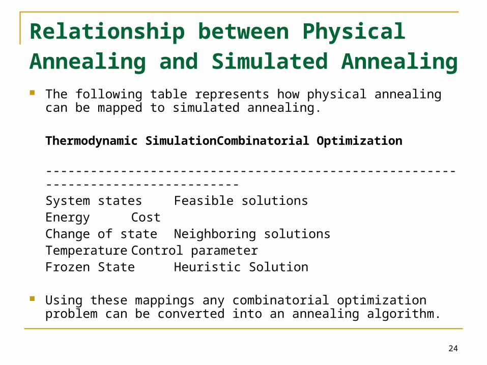
Relationship between Physical Annealing and Simulated Annealing The following table represents how physical annealing can be

mapped to simulated annealing.

Thermodynamic Simulation Combinatorial Optimization

---------------------------------------------------------------------------------System states Feasible solutionsEnergy CostChange of state Neighboring solutionsTemperature Control parameterFrozen State Heuristic Solution

Using these mappings any combinatorial optimization problem can be converted into an annealing algorithm.

25

Simulated Annealing Algorithm

To apply the SA algorithm, we have to represent the problem in the local search framework, by defining a solution space a neighborhood structure a cost function.

This essentially defines a solution landscape which is searched by moving from the current solution to a neighboring solution.

The outline of the basic procedure for SA algorithm is as follows

26

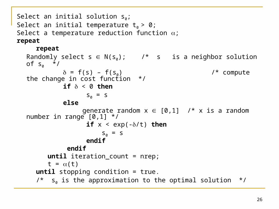
Select an initial solution s0;Select an initial temperature t0 > 0;Select a temperature reduction function ;repeat repeat

Randomly select s N(s0); /* s is a neighbor solution of s0 */ = f(s) – f(s0) /* compute the change in cost function */ if < 0 then s0 = s else generate random x [0,1] /* x is a random number in range [0,1] */ if x < exp(-/t) then s0 = s endif endif until iteration_count = nrep; t = (t) until stopping condition = true. /* s0 is the approximation to the optimal solution */

27

SA algorithm (cont.) Potential moves are sampled randomly and all improving moves

are accepted automatically. Other moves are accepted with probability exp(-/t), where is the change in cost function and t is a control parameter.

The quality of solutions is sensitive to the way in which the temperature parameter is adjusted - the cooling schedule. This is defined by the starting temperature t0, the stopping conditions, the reduction function the number of repetitions at each temperature, nrep.

These values are problem-specific as they must be chosen with respect to the shape of the solution landscape

28

Cooling Schedule The cooling schedule of a simulated annealing algorithm consists

of four components: Starting Temperature, Final Temperature, Temperature Decrement, Iterations at each temperature

Starting Temperature The t0 must be hot enough to allow a move to almost any

neighborhood state. If this is not done then the ending solution will be the same (or very close) to the starting solution. Alternatively, we will simply implement a hill climbing algorithm.

However, if t0 starts at too high a value, then the search can move to any neighbor and thus transform the search (at least in the early stages) into a random search.

Effectively, the search will be random until the temperature is cool enough to start acting as a SA algorithm.

29

Starting temperature (cont.) The problem is finding the correct starting temperature. At

present, there is no known method for finding a suitable starting temperature for a whole range of problems.

If we know the maximum distance (cost function difference) between one neighbor and another then we can use this information to calculate a starting temperature.

Another method is to start with a very high temperature and cool it rapidly until about 60% of worse solutions are being accepted. This forms the real starting temperature and it can now be cooled more slowly.

30

Final temperature

It is usual to let the temperature decrease until it reaches zero. However, this can make the algorithm run for a lot longer, especially when a geometric cooling schedule is being used.

In practice, it is not necessary to let the temperature reach zero because as it approaches zero, the chances of accepting a worse move are almost the same as the temperature being equal to zero.

Therefore, the stopping criteria can either be a suitable low temperature or when the system is “frozen” at the current temperature (i.e. no

better or worse moves are being accepted).

31

Temperature Decrement Theory states that we should allow enough iterations at each

temperature so that the system stabilizes at that temperature. Unfortunately, theory also states that the number of iterations at each temperature to achieve this might be exponential to the problem size. As this is impractical we need to compromise. We can do this by doing either a larger number of iterations at a few temperature, or a small number of iterations at many temperatures, or a balance between them.

One way to decrement the temperature is a simple linear method. An alternative is a geometric decrement where t = t where < 1. Experience has shown that should be between 0.8 and 0.99, with

better results being found in the higher end of the range.

32

Problem Specific Decisions Iterations at each Temperature

A constant number of iterations at each temperature is an obvious scheme.

The cost function In defining this cost function we need to ensure that it

represents the problem we are trying to solve. It’s also important that the cost function can be calculated

as efficiently as possible, as it will be calculated at every iteration of the algorithm. However, the cost function is often a bottleneck and it may sometimes be necessary to use Delta Evaluation: the difference between the current solution

and the neighborhood solution is evaluated. Partial Evaluation: a simplified evaluation function is used that

does not give an exact result but gives a good indication as to the quality of the solution.

33

Neighborhood Structure The problem is how we move from one state to another. This

means that you have to define a neighborhood. That is, when you are in a certain state, what other states are reachable.

In a problem such as a course timetabling problem, the neighborhood function could be defined as swapping a lecture from one room to another.

Some results have shown that the neighborhood structure should be symmetric. That is, if you move from state i to state j then it must be possible to move from state j to state i.

It has been found, however, that a weaker condition can hold in order to ensure convergence. That is, that every state must be reachable from every other. Therefore, it is important, when thinking about your problem to ensure that this condition is met.

34

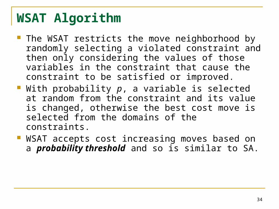
WSAT Algorithm The WSAT restricts the move neighborhood by

randomly selecting a violated constraint and then only considering the values of those variables in the constraint that cause the constraint to be satisfied or improved.

With probability p, a variable is selected at random from the constraint and its value is changed, otherwise the best cost move is selected from the domains of the constraints.

WSAT accepts cost increasing moves based on a probability threshold and so is similar to SA.

35

WSAT vs. SA

However WSAT differs from SA in three areas: In WSAT only variables involved in constraint

violations are considered for changing. The value of probability p is fixed. The WSAT cost function select moves on the basis

of minimizing the number of constraints a move will violate.

36

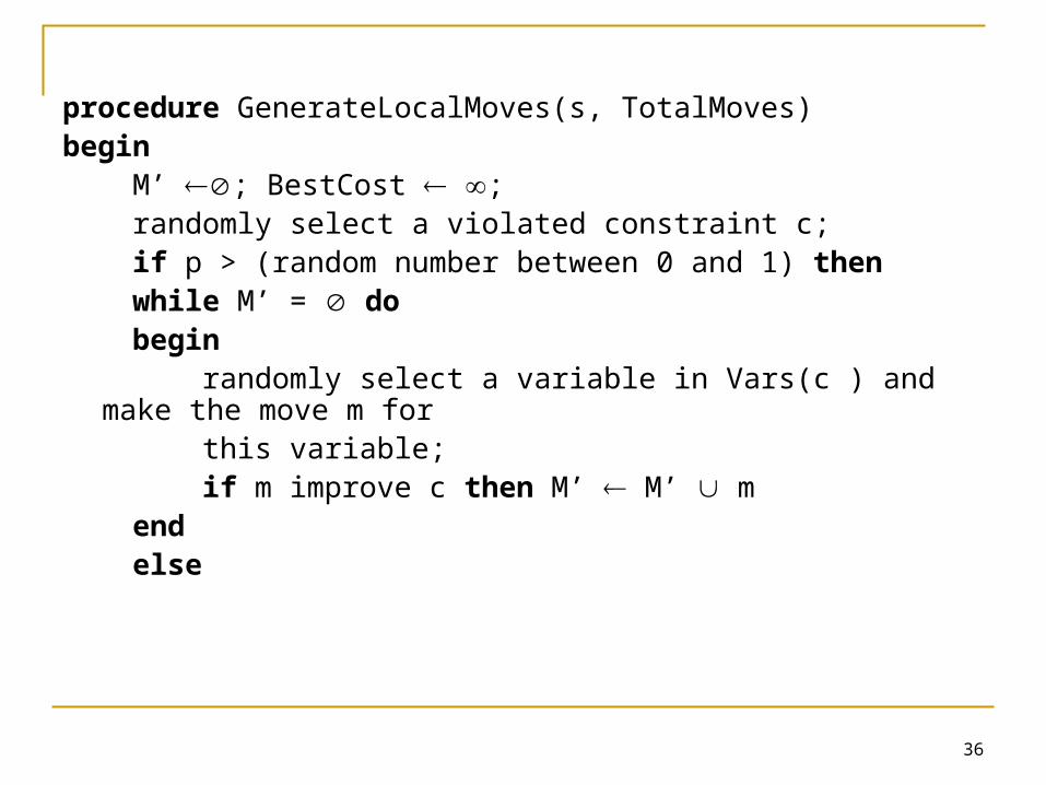
procedure GenerateLocalMoves(s, TotalMoves)begin M’ ; BestCost ; randomly select a violated constraint c; if p > (random number between 0 and 1) then while M’ = do begin randomly select a variable in Vars(c ) and make the move m for this variable; if m improve c then M’ M’ m end else

37

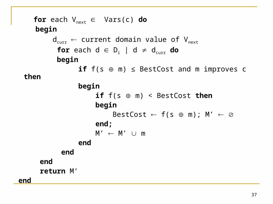
for each Vnext Vars(c) do begin

dcurr current domain value of Vnext

for each d Di | d dcurr do begin if f(s m) ≤ BestCost and m improves c then begin if f(s m) < BestCost then begin BestCost f(s m); M’ end; M’ M’ m end end end return M’ end

38

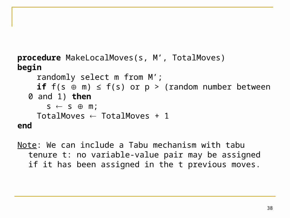
procedure MakeLocalMoves(s, M’, TotalMoves)begin randomly select m from M’; if f(s m) ≤ f(s) or p > (random number between 0 and 1) then s s m; TotalMoves TotalMoves + 1end

Note: We can include a Tabu mechanism with tabu tenure t: no variable-value pair may be assigned if it has been assigned in the t previous moves.

39

CONCLUSIONS Properties of Local Search Techniques The idea of local search is to find a short-cut to an

answer by descending quickly to the nearest minimum cost solution in the search space.

It avoid the expense of a systematic search by exploiting the cost landscape of the search space.

The average-case performance of a local search depends on the particular cost landscape of the problem.

Therefore, local search techniques are evaluated empirically on a problem-by-problem basis rather than using formal analysis.

Local search techniques are also called a kind of metaheuristics.

40

Cooperation of Local Search and Constraint Programming Algorithms for solving CSP fall into one of two main

families: systematic algorithm (BC-FC, BM, BJ, CBJ) local search.

Both families have their advantages. Several research works have studied cooperation

between local search and systematic search. These hybrid approaches have led to good results

on large scale problems.

41

Three hybrid approaches

Three categories of hybrid approaches: performing a local search before or after a systematic

search. (e.g, Constraint Programming and then SA for Exam Timetabling)

performing a systematic search improved with a local search at some point of the search: LS used as a way to improve some of the nodes of the search tree or to explore a set of paths close to the path selected by a

greedy algorithm in the search tree. performing an overall local search, and using systematic

search either to select candidate neighbor or to prune the search space.

42

Metaheuristics “Metaheuristic is an iterative process which guides a

subordinate heuristic by combining intelligently different concepts for exploring and exploiting the search spaces using learning strategies to structure information in order to find efficiently near-optimal solutions.”

Includes: Hill-Climbing SA Tabu Search Variable Neighborhood Search Genetic Algorithm Ant Colony Optimization (ACO) Artificial Immune Systems