1 Chapter 5 Correlation IIntroduction to Correlation and Regression A.Describing the Linear Relationship Between Two Variables, X and Y 1.Pearson product-moment.

1

Chapter 5

Correlation

I Introduction to Correlation and Regression

A. Describing the Linear Relationship Between Two Variables, X and Y

1. Pearson product-moment correlation coefficient (r)

2

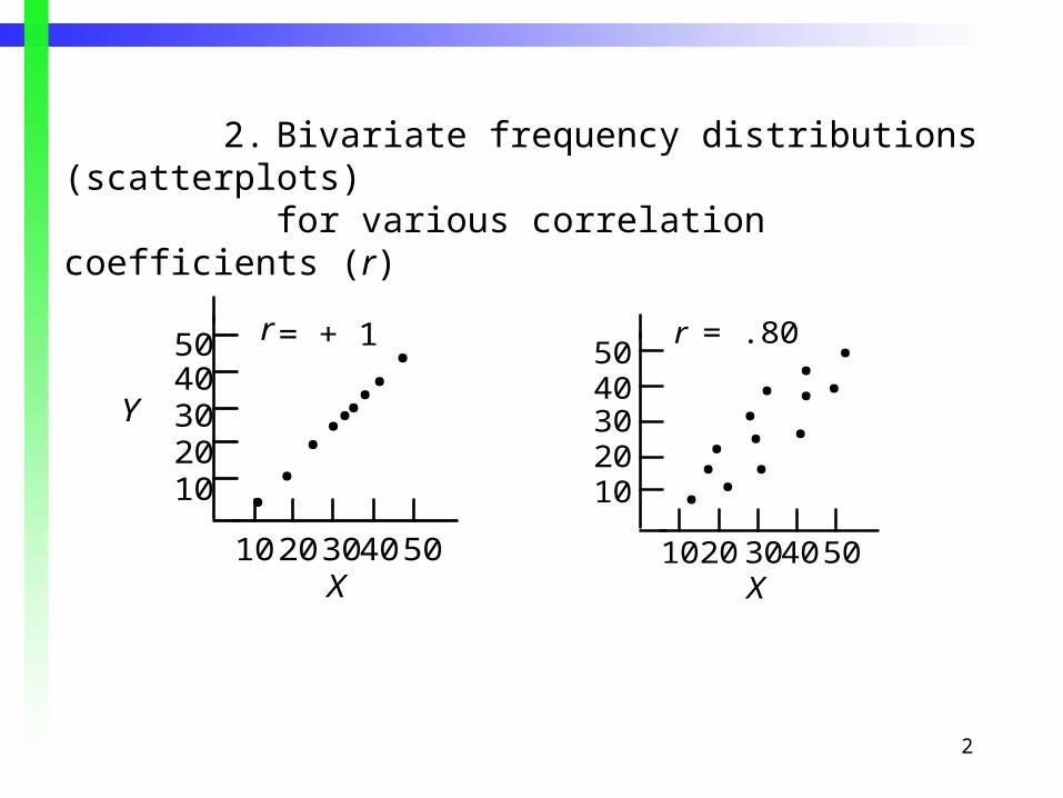
2. Bivariate frequency distributions (scatterplots)for various correlation coefficients (r)

5040302010

5040302010

Y

X

r= + 1

••

••

••

••

•

5040302010

5040302010X

•

••

• •

••

•••

•• •

r = .80

3

5040302010X

Y••••••••

••

•

••

•

•

•

•

•

•

•5040302010

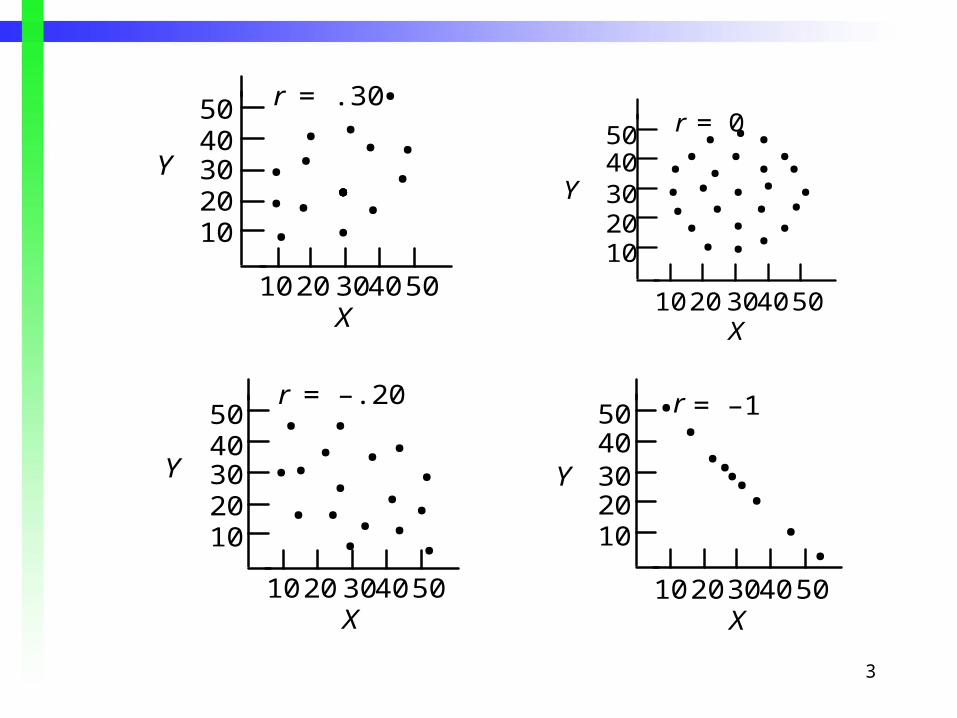
r = .30

= 0

5040302010X

r

•

•••

••

••

•

•

•••

•

•

•

••

••

•

•

••

•

Y

5040302010

5040302010X

Y•

•

•••

•• •

•

•

• •

••

•

••

5040302010

r = –.20

= –1

5040302010X

r

••

•••

••

••Y

5040302010

4

3. Upper and lower limits for r: +1 to –1

B. Correlation and Regression Distinguished

1. Characteristics of regression situations

One dependent variable, Y, and one or more independent variables, X

Levels of independent variables are

selected in advance

The value of the dependent variable for a given level of the independent variable is free

to vary

5

The researcher is primarily interested in predicting Y from a knowledge of X

2. Characteristics of correlation situation

Neither variable is considered the independent variable

The researcher is primarily interested in assessing the strength of the relationship between X and Y

X and Y are both free to vary

6

II Correlation

A. Formula for Pearson Product-Moment Correlation Coefficient

r SXY

SX SY

( X i X )(Yi Y )i1

n

n

( X i X )2

i1

n

n

(Yi Y )2

i1

n

n

7

1. Understanding the formula for r; what the numerator tells you

Covariance

SXY

( X i X )(Yi Y )i1

n

n

Information in the cross products

( X i X )(Yi Y )

i1

n

8

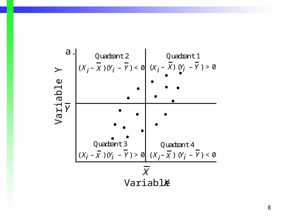
••••••••••••••••••iiQuadrant 1(X – X) (Y – Y) > 0iiQuadrant 3(X – X) (Y – Y) > 0Variable YY Quadrant 2(Xi – X) (Yi – Y) < 0Quadrant 4 (Xi – X) (Yi – Y) < 0XVariable Xa.

•

••

••

•

•

•

••

••• •

••

• •

i i

Quadrant 1

(X – X) (Y – Y ) > 0

i i

Quadrant 3

( X – X ) (Y – Y ) > 0

Var

iabl

e Y

Y

Quadrant 2

( Xi – X ) (Yi – Y ) < 0

Quadrant 4

( Xi – X ) (Yi – Y ) < 0

XVariable X

a.

9

••••

•

•

•

•

••

••

•

•

••••

i i

Quadrant 1

(X – X) (Y – Y ) > 0

i i

Quadrant 3

( X – X ) (Y – Y ) > 0

Var

iabl

e Y

Y

Quadrant 2

(Xi – X ) (Yi – Y ) < 0

Quadrant 4

(Xi – X) (Yi – Y ) < 0

XVariable X

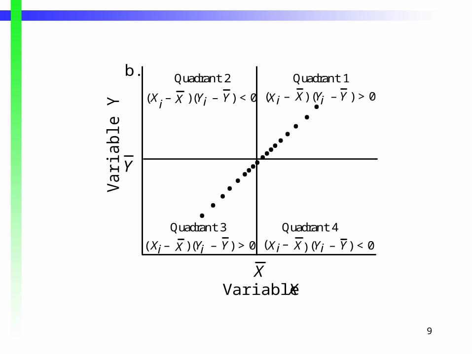
b.

10

2. If the majority of the data points fall in quadrants1 and 3, the cross product is positive and r > 0

3. If the majority of the data points fall in quadrants2 and 4, the cross product is negative and r < 0

4. If the data points are equally dispersed over the four quadrants, the cross product equals zero and r = 0

5. The cross product is largest when the data pointsfall on a straight line

6. The cross product is small when the data pointsfall in an elongated circle (ellipse)

11

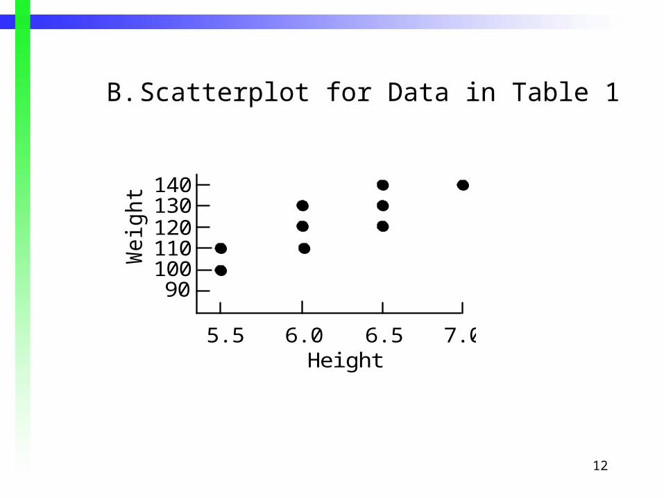
Table 1. Height and Weight of Girl’s Basketball Team

1 7.0 140 .64 289 13.62 6.5 130 .09 49 2.13 6.5 140 .09 289 5.14 6.5 130 .09 49 2.15 6.5 120 .09 9 –0.96 6.0 120 .04 9 0.67 6.0 130 .04 49 –1.48 6.0 110 .04 169 2.69 5.5 100 .49 529 16.1

10 5.5 110 .49 169 9.1

X i

Yi Girl ( X i X )2

(Yi Y )2

( X i X )(Yi Y )

(1) (2) (3) (4) (5)

X 6.2 Y 123 2.10 1610 49.0

(6)

12

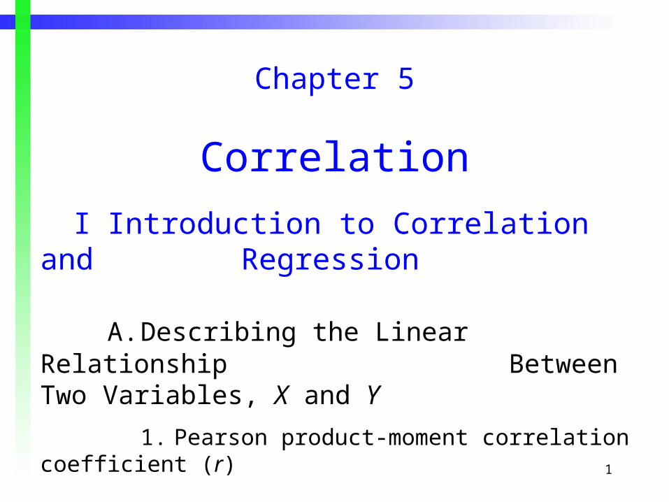
B. Scatterplot for Data in Table 1

5.5 6.0 6.5 7.0

90100110120130140

Height

Wei

ght

13

r

( X i X )(Yi Y )i1

n

n

( X i X )2

i1

n

n

(Yi Y )2

i1

n

n

49.0

10

2.10

10

1610

10

6.30

5.8152.84

C. Computation of r for Data in Table 1

14

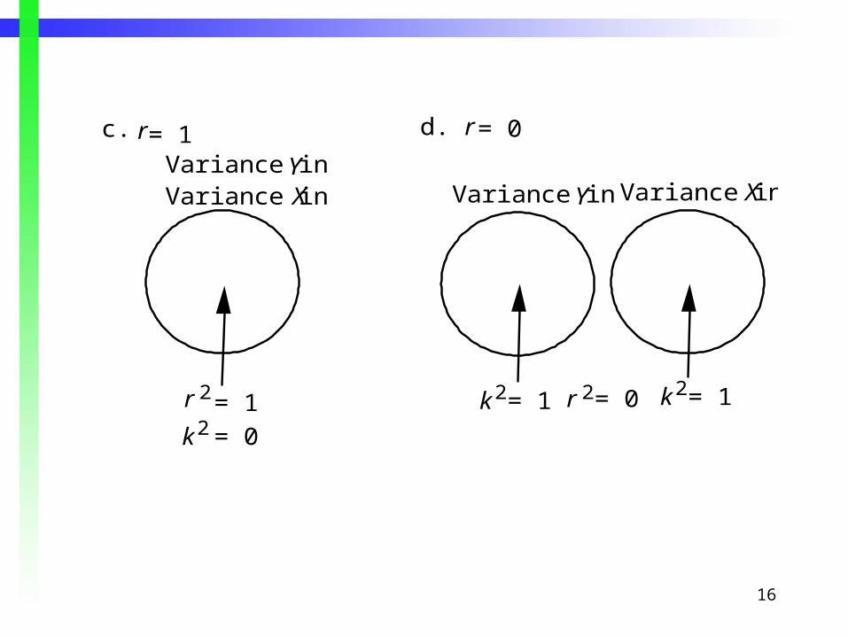
III Interpretation of the Correlation Coefficient

A. Coefficient of Determination, r2 , and

Nondetermination, k2

Total Y variance

expressed as a

proportion

Proportion of Y

variance explained

by X variance

Proportion of Y

variance not explained

by X variance

SY2

SY2 r 2 k 2

15

B. Visual Representation of r2 and k2

b.

Variance in Y Variance in X

k2 = .84 k2 = .84 r2 = .16

r = .40 a.Variance in Y Variance in X

k2 = .29 k2 = .29 r2 = .71

r = .84

16

c. d.= 1r = 0r

= 1k 2

= 0k 2

= 0r 2= 1r 2

Variance in YVariance in Y

Variance in XVariance in X

= 1k 2

17

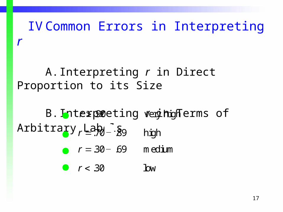
IV Common Errors in Interpreting r

A. Interpreting r in Direct Proportion to its Size

B. Interpreting r in Terms of Arbitrary Labels

r .90 very high

r .70 Š .89 high

r .30 Š .69 medium

r .30 low

18

1. Typical reliability coefficients

2. Typical validity coefficients

C. Inferring Causation from Correlation

V Some Factors That Affect the Correlation Coefficient

19

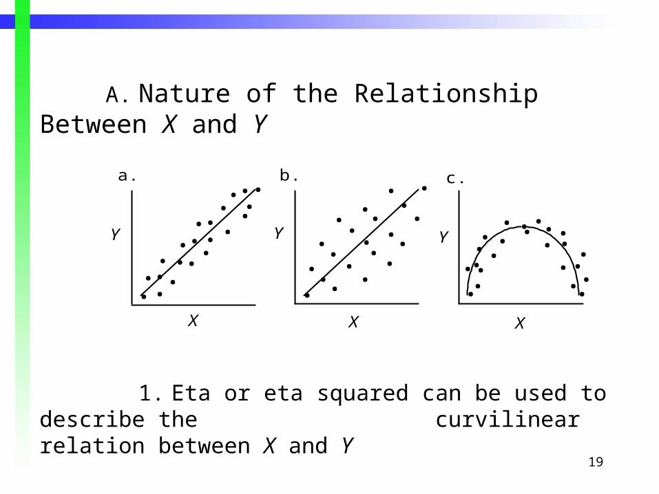
A. Nature of the Relationship Between X and Y

•

•

••

•• •

•

•

•

••

•

•

••

•

•

•••

•• ••

• ••

•

•

•

•

•

•

••

• ••

•

••

•••

•••

•

•

••

•• •

••

•• •

••

•

•

•

a. b. c.

Y Y Y

X X X

1. Eta or eta squared can be used to describe the curvilinear relation between X and Y

20

B. Truncated Range

110

100

90

80

70

60

504030 60 70 80

Aptitude score

Pro

duct

ion

units

per

day

90

•

• •

••

•

•

•

• •

•••

•••

••

•

••

•

••

•

••

••

••

•

••

•

•

•

•

•

Y

X

Prod

ucti

on u

nits

per

day

21

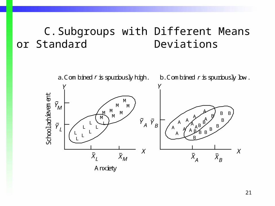
C. Subgroups with Different Means or Standard Deviations

A

A AAA

A

A

A

AA

A B

B

B

BB B

BB

B

BB

B

LL

L

L

LL

L

L

MMM

MMM

MM

Anxiety

Scho

ol a

chie

vem

ent

X

Y Y

YM–

YA

–Y

B–

XB–XM

–X

A–

YL–

XL– X

a. Combined is spuriously high.r b. Combined is spuriously low.r

22

X

Y Y

X

A A

AAB

A

AA

A

ABAAAA

A A

A A

A

AA

AA

A

AA

A

A

AA

ABB

BBB

BB BB

B BB

BBB

B

B

B

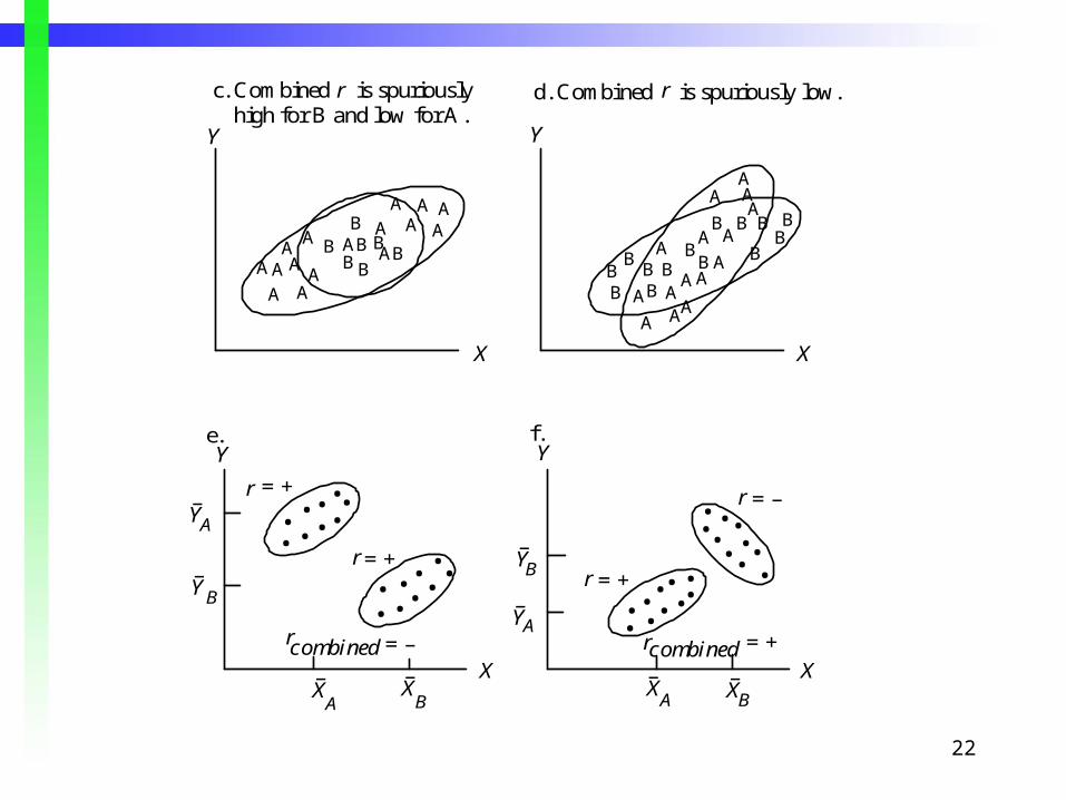
high for B and low for A.c. Combined is spuriouslyr d. Combined is spuriously low.r

AB

X

Y Y

YA–

AY–

BY–

XB–X

B

–X

A–

YB–

XA

– X

•••

••

•

••• •

• • •••

•

• •• • ••••

•••

•• •

•

•• ••

•• •

= – = +

e. f.

= +r= +r

r= +r

rcombined rcombined

= –

23

D. Discontinuous Distribution

16

1618

18

20

20

22

22 24

2426

26

28

28

30

30 32

3234

34 36

3638

38 40

404244

•

••

•

••

•

•

Region of discontinuity

Father's authoritarianism

Son

's a

utho

rita

rian

ism

24

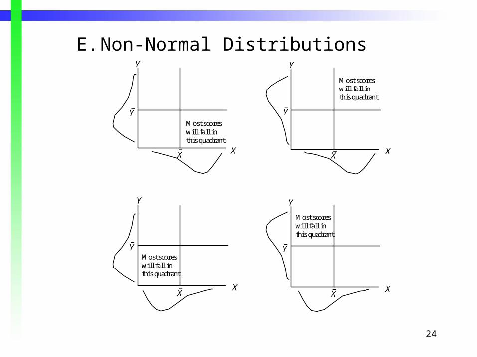
E. Non-Normal Distributions

X

Y Y

Y

XX

X

Y

Most scores will fall in this quadrant

Most scores will fall in this quadrant

Most scores will fall in this quadrant

Most scores will fall in this quadrant

–X

Y–

Y–

Y–Y

–

–X

–X

–X

25

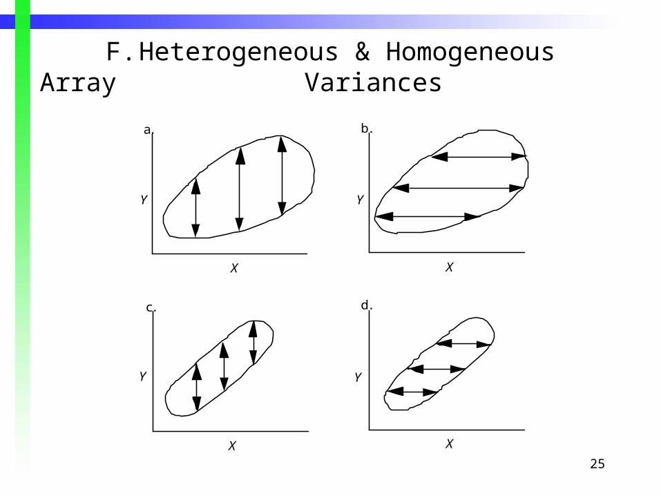
F. Heterogeneous & Homogeneous Array Variances

X X

XX

Y

YY

Y

a. b.

c. d.

26

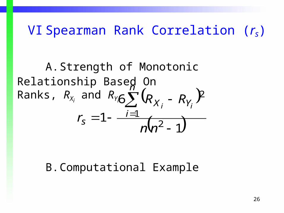
VI Spearman Rank Correlation (rs)

A. Strength of Monotonic Relationship Based On Ranks, RXi

and RYi

B. Computational Example

1

6

12

1

2

nn

RR

r

n

iYX

s

ii

27

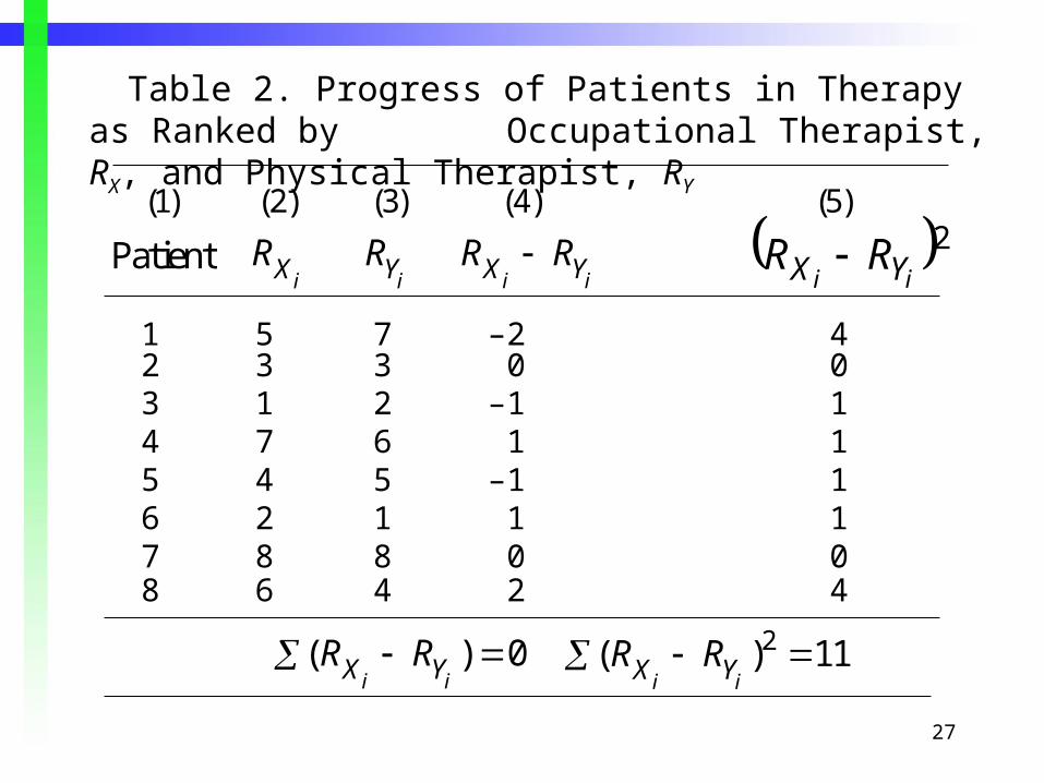
Table 2. Progress of Patients in Therapy as Ranked by Occupational Therapist, RX, and Physical Therapist, RY

1 5 7 –2 42 3 3 0 03 1 2 –1 14 7 6 1 15 4 5 –1 16 2 1 1 17 8 8 0 08 6 4 2 4

Patient RX i

RYi RX i

RYi

(1) (2) (3) (4)

(RX i

RYi) 0

(RX i

RYi)2 11

(5)

2ii YX RR

28

C. Computation of rs

rs 1 6(11)

8 (8)2 1

1 66

504.87

1. Dealing with tied ranks

1

6

12

1

2

nn

RR

r

n

iYX

s

ii

29

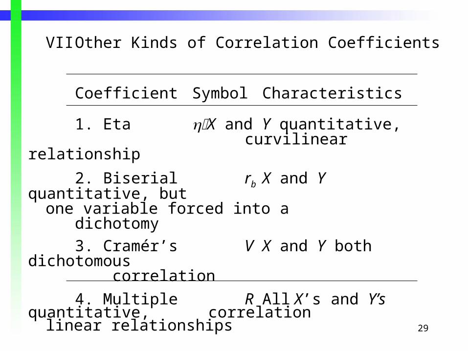
VII Other Kinds of Correlation Coefficients

Coefficient Symbol Characteristics

1. Eta X and Y quantitative,curvilinear relationship

2. Biserial rb X and Y quantitative, but one variable forced into a

dichotomy

3. Cramér’s V X and Y both dichotomous correlation

4. Multiple R All X’s and Y’s quantitative, correlation linear relationships