1 Chapter 1. Introduction Motivation: Why data mining? What is data mining? Data Mining: On what kind of data? Data mining functionality Major issues in.

1

Chapter 1. Introduction

Motivation: Why data mining?

What is data mining?

Data Mining: On what kind of data?

Data mining functionality

Major issues in data mining

2

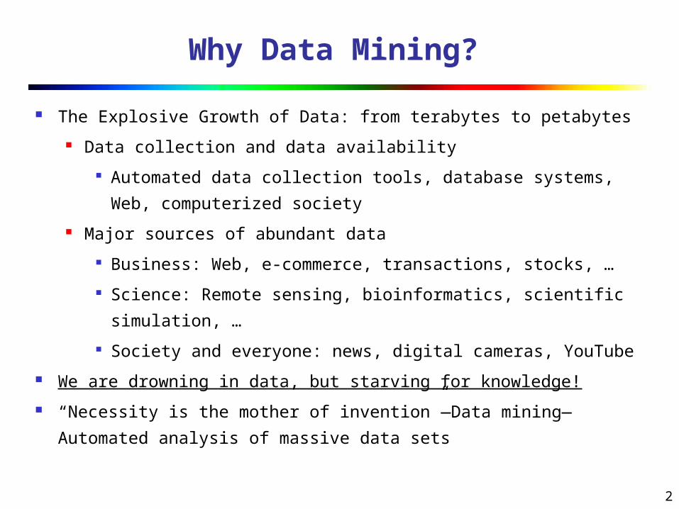
Why Data Mining?

The Explosive Growth of Data: from terabytes to petabytes

Data collection and data availability

Automated data collection tools, database systems, Web,

computerized society

Major sources of abundant data

Business: Web, e-commerce, transactions, stocks, …

Science: Remote sensing, bioinformatics, scientific

simulation, …

Society and everyone: news, digital cameras, YouTube

We are drowning in data, but starving for knowledge!

“Necessity is the mother of invention”—Data mining—

Automated analysis of massive data sets

3

Evolution of Database Technology

1960s: Data collection, database creation, IMS and network DBMS

1970s: Relational data model, relational DBMS implementation

1980s: RDBMS, advanced data models (extended-relational, OO, deductive,

etc.) Application-oriented DBMS (spatial, scientific, engineering, etc.)

1990s: Data mining, data warehousing, multimedia databases, and Web

databases 2000s

Stream data management and mining Data mining and its applications Web technology (XML, data integration) and global information

systems

4

What Is Data Mining?

Data mining (knowledge discovery from data) Extraction of interesting (non-trivial, implicit, previously

unknown and potentially useful) patterns or knowledge from huge amount of data

Data mining: a misnomer?

Alternative names Knowledge discovery (mining) in databases (KDD),

knowledge extraction, data/pattern analysis, data archeology, data dredging, information harvesting, business intelligence, etc.

Watch out: Is everything “data mining”? Simple search and query processing (Deductive) expert systems

5

Knowledge Discovery (KDD) Process

Data mining—core of knowledge discovery process

Data Cleaning

Data Integration

Databases

Data Warehouse

Task-relevant Data

Selection

Data Mining

Pattern Evaluation

6

KDD Process: Several Key Steps

Learning the application domain relevant prior knowledge and goals of application

Creating a target data set: data selection Data cleaning and preprocessing: (may take 60% of effort!) Data reduction and transformation

Find useful features, dimensionality/variable reduction, invariant representation

Choosing functions of data mining summarization, classification, regression, association, clustering

Choosing the mining algorithm(s) Data mining: search for patterns of interest Pattern evaluation and knowledge presentation

visualization, transformation, removing redundant patterns, etc. Use of discovered knowledge

7

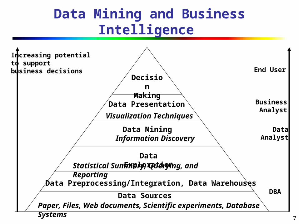
Data Mining and Business Intelligence

Increasing potentialto supportbusiness decisions End User

Business Analyst

DataAnalyst

DBA

Decision

MakingData Presentation

Visualization Techniques

Data MiningInformation Discovery

Data ExplorationStatistical Summary, Querying, and Reporting

Data Preprocessing/Integration, Data Warehouses

Data SourcesPaper, Files, Web documents, Scientific experiments, Database Systems

8

Data Mining: Confluence of Multiple Disciplines

Data Mining

Database Technology Statistics

MachineLearning

PatternRecognition

AlgorithmOther

Disciplines

Visualization

9

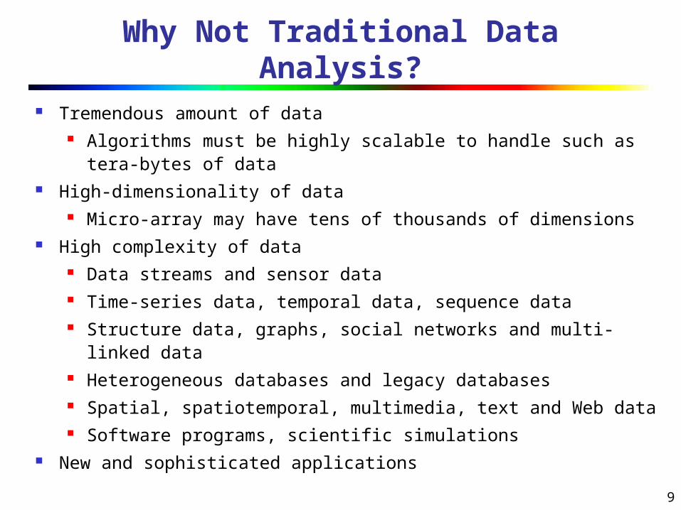
Why Not Traditional Data Analysis?

Tremendous amount of data Algorithms must be highly scalable to handle such as tera-

bytes of data High-dimensionality of data

Micro-array may have tens of thousands of dimensions High complexity of data

Data streams and sensor data Time-series data, temporal data, sequence data Structure data, graphs, social networks and multi-linked data Heterogeneous databases and legacy databases Spatial, spatiotemporal, multimedia, text and Web data Software programs, scientific simulations

New and sophisticated applications

10

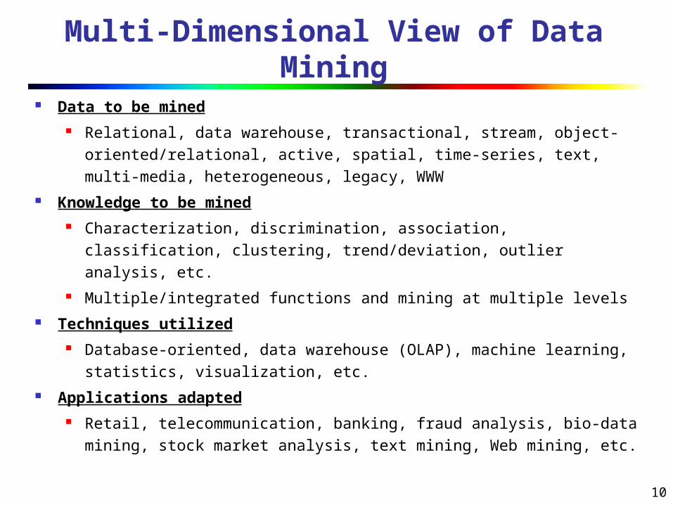
Multi-Dimensional View of Data Mining

Data to be mined Relational, data warehouse, transactional, stream, object-

oriented/relational, active, spatial, time-series, text, multi-media, heterogeneous, legacy, WWW

Knowledge to be mined Characterization, discrimination, association, classification,

clustering, trend/deviation, outlier analysis, etc. Multiple/integrated functions and mining at multiple levels

Techniques utilized Database-oriented, data warehouse (OLAP), machine learning,

statistics, visualization, etc. Applications adapted

Retail, telecommunication, banking, fraud analysis, bio-data mining, stock market analysis, text mining, Web mining, etc.

11

Data Mining: Classification Schemes

General functionality

Descriptive data mining

Predictive data mining

Different views lead to different classifications

Data view: Kinds of data to be mined

Knowledge view: Kinds of knowledge to be

discovered

Method view: Kinds of techniques utilized

Application view: Kinds of applications adapted

12

Data Mining: On What Kinds of Data?

Database-oriented data sets and applications

Relational database, data warehouse, transactional database

Advanced data sets and advanced applications

Data streams and sensor data

Time-series data, temporal data, sequence data (incl. bio-

sequences)

Structure data, graphs, social networks and multi-linked data

Object-relational databases

Heterogeneous databases and legacy databases

Spatial data and spatiotemporal data

Multimedia database

Text databases

The World-Wide Web

13

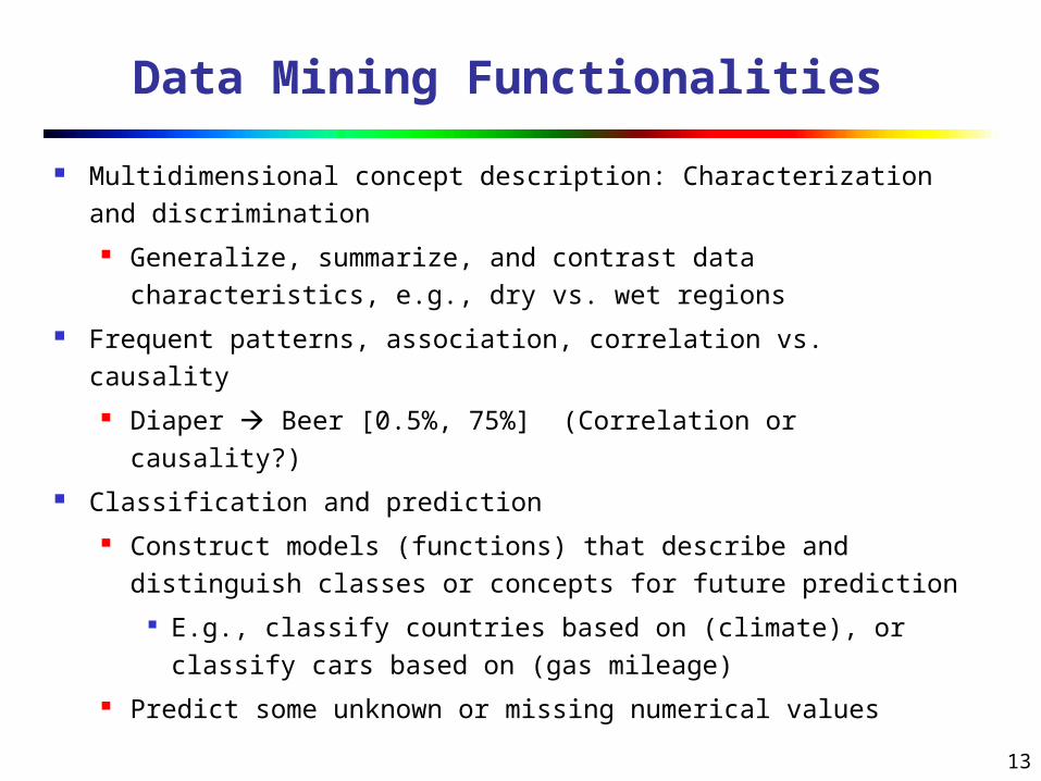
Data Mining Functionalities

Multidimensional concept description: Characterization and discrimination Generalize, summarize, and contrast data

characteristics, e.g., dry vs. wet regions Frequent patterns, association, correlation vs. causality

Diaper Beer [0.5%, 75%] (Correlation or causality?) Classification and prediction

Construct models (functions) that describe and distinguish classes or concepts for future prediction

E.g., classify countries based on (climate), or classify cars based on (gas mileage)

Predict some unknown or missing numerical values

14

Data Mining Functionalities (2)

Cluster analysis Class label is unknown: Group data to form new classes, e.g.,

cluster houses to find distribution patterns Maximizing intra-class similarity & minimizing interclass similarity

Outlier analysis Outlier: Data object that does not comply with the general behavior

of the data Noise or exception? Useful in fraud detection, rare events analysis

Trend and evolution analysis Trend and deviation: e.g., regression analysis Sequential pattern mining: e.g., digital camera large SD memory Periodicity analysis Similarity-based analysis

Other pattern-directed or statistical analyses

15

Major Issues in Data Mining

Mining methodology Mining different kinds of knowledge from diverse data types, e.g., bio,

stream, Web Performance: efficiency, effectiveness, and scalability Pattern evaluation: the interestingness problem Incorporation of background knowledge Handling noise and incomplete data Parallel, distributed and incremental mining methods Integration of the discovered knowledge with existing one: knowledge

fusion User interaction

Data mining query languages and ad-hoc mining Expression and visualization of data mining results Interactive mining of knowledge at multiple levels of abstraction

Applications and social impacts Domain-specific data mining & invisible data mining Protection of data security, integrity, and privacy

16

Are All the “Discovered” Patterns Interesting?

Data mining may generate thousands of patterns: Not all of

them are interesting Suggested approach: Human-centered, query-based, focused

mining

Interestingness measures A pattern is interesting if it is easily understood by humans, valid

on new or test data with some degree of certainty, potentially

useful, novel, or validates some hypothesis that a user seeks to

confirm

Objective vs. subjective interestingness measures Objective: based on statistics and structures of patterns, e.g.,

support, confidence, etc.

Subjective: based on user’s belief in the data, e.g.,

unexpectedness, novelty, actionability, etc.

17

Find All and Only Interesting Patterns?

Find all the interesting patterns: Completeness Can a data mining system find all the interesting patterns?

Do we need to find all of the interesting patterns? Heuristic vs. exhaustive search Association vs. classification vs. clustering

Search for only interesting patterns: An optimization problem Can a data mining system find only the interesting

patterns? Approaches

First general all the patterns and then filter out the uninteresting ones

Generate only the interesting patterns—mining query optimization

18

Why Data Mining Query Language?

Automated vs. query-driven? Finding all the patterns autonomously in a database?—

unrealistic because the patterns could be too many but uninteresting

Data mining should be an interactive process User directs what to be mined

Users must be provided with a set of primitives to be used to communicate with the data mining system

Incorporating these primitives in a data mining query language More flexible user interaction Foundation for design of graphical user interface Standardization of data mining industry and practice

19

Primitives that Define a Data Mining Task

Task-relevant data Database or data warehouse name Database tables or data warehouse cubes Condition for data selection Relevant attributes or dimensions Data grouping criteria

Type of knowledge to be mined Characterization, discrimination, association, classification,

prediction, clustering, outlier analysis, other data mining tasks

Background knowledge Pattern interestingness measurements Visualization/presentation of discovered patterns

20

Primitive 3: Background Knowledge

A typical kind of background knowledge: Concept hierarchies Schema hierarchy

E.g., street < city < province_or_state < country Set-grouping hierarchy

E.g., {20-39} = young, {40-59} = middle_aged Operation-derived hierarchy

email address: [email protected]

login-name < department < university < country Rule-based hierarchy

low_profit_margin (X) <= price(X, P1) and cost (X, P2) and

(P1 - P2) < $50

mailto:[email protected]

21

Primitive 4: Pattern Interestingness

Measure

Simplicity

e.g., (association) rule length, (decision) tree size Certainty

e.g., confidence, P(A|B) = #(A and B)/ #(B), classification reliability or accuracy, certainty factor, rule strength, rule quality, discriminating weight, etc.

Utility

potential usefulness, e.g., support (association), noise threshold (description)

Novelty

not previously known, surprising (used to remove redundant rules, e.g., Illinois vs. Champaign rule implication support ratio)

22

Primitive 5: Presentation of Discovered Patterns

Different backgrounds/usages may require different forms of

representation

E.g., rules, tables, crosstabs, pie/bar chart, etc.

Concept hierarchy is also important

Discovered knowledge might be more understandable

when represented at high level of abstraction

Interactive drill up/down, pivoting, slicing and dicing

provide different perspectives to data

Different kinds of knowledge require different

representation: association, classification, clustering, etc.

23

DMQL—A Data Mining Query Language

Motivation A DMQL can provide the ability to support ad-hoc and

interactive data mining By providing a standardized language like SQL

Hope to achieve a similar effect like that SQL has on relational database

Foundation for system development and evolution Facilitate information exchange, technology

transfer, commercialization and wide acceptance Design

DMQL is designed with the primitives described earlier

24

An Example Query in DMQL

25

Other Data Mining Languages & Standardization Efforts

Association rule language specifications MSQL (Imielinski & Virmani’99)

MineRule (Meo Psaila and Ceri’96)

Query flocks based on Datalog syntax (Tsur et al’98)

OLEDB for DM (Microsoft’2000) and recently DMX (Microsoft

SQLServer 2005) Based on OLE, OLE DB, OLE DB for OLAP, C#

Integrating DBMS, data warehouse and data mining

DMML (Data Mining Mark-up Language) by DMG (www.dmg.org) Providing a platform and process structure for effective data

mining

Emphasizing on deploying data mining technology to solve

business problems

26

Integration of Data Mining and Data Warehousing

Data mining systems, DBMS, Data warehouse systems

coupling

No coupling, loose-coupling, semi-tight-coupling, tight-coupling

On-line analytical mining data

integration of mining and OLAP technologies

Interactive mining multi-level knowledge

Necessity of mining knowledge and patterns at different levels

of abstraction by drilling/rolling, pivoting, slicing/dicing, etc.

Integration of multiple mining functions

Characterized classification, first clustering and then

association

27

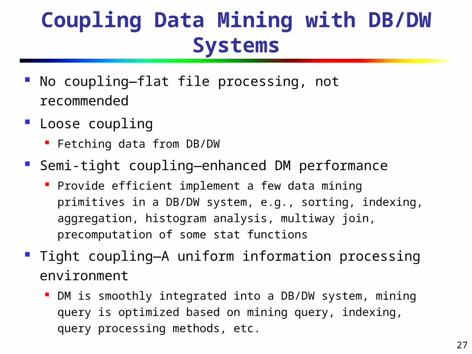
Coupling Data Mining with DB/DW Systems

No coupling—flat file processing, not recommended Loose coupling

Fetching data from DB/DW

Semi-tight coupling—enhanced DM performance Provide efficient implement a few data mining primitives in

a DB/DW system, e.g., sorting, indexing, aggregation, histogram analysis, multiway join, precomputation of some stat functions

Tight coupling—A uniform information processing environment DM is smoothly integrated into a DB/DW system, mining

query is optimized based on mining query, indexing, query processing methods, etc.

28

Architecture: Typical Data Mining System

data cleaning, integration, and selection

Database or Data Warehouse Server

Data Mining Engine

Pattern Evaluation

Graphical User Interface

Knowledge-Base

Database Data Warehouse

World-WideWeb

Other InfoRepositories

29

What is Data Warehouse?

Defined in many different ways, but not rigorously.

A decision support database that is maintained separately from

the organization’s operational database

Support information processing by providing a solid platform of

consolidated, historical data for analysis.

“A data warehouse is a subject-oriented, integrated, time-

variant, and nonvolatile collection of data in support of

management’s decision-making process.”—W. H. Inmon

Data warehousing:

The process of constructing and using data warehouses

30

Data Warehouse—Subject-Oriented

Organized around major subjects, such as

customer, product, sales

Focusing on the modeling and analysis of data for

decision makers, not on daily operations or

transaction processing

Provide a simple and concise view around

particular subject issues by excluding data that

are not useful in the decision support process

31

Data Warehouse—Integrated

Constructed by integrating multiple, heterogeneous data sources relational databases, flat files, on-line transaction records

Data cleaning and data integration techniques are applied. Ensure consistency in naming conventions, encoding

structures, attribute measures, etc. among different data sources

E.g., Hotel price: currency, tax, breakfast covered, etc.

When data is moved to the warehouse, it is converted.

32

Data Warehouse—Time Variant

The time horizon for the data warehouse is significantly longer than that of operational systems Operational database: current value data Data warehouse data: provide information from a

historical perspective (e.g., past 5-10 years)

Every key structure in the data warehouse Contains an element of time, explicitly or implicitly But the key of operational data may or may not contain

“time element”

33

Data Warehouse—Nonvolatile

A physically separate store of data transformed

from the operational environment

Operational update of data does not occur in the

data warehouse environment Does not require transaction processing, recovery, and

concurrency control mechanisms

Requires only two operations in data accessing:

initial loading of data and access of data

34

Data Warehouse vs. Heterogeneous DBMS

Traditional heterogeneous DB integration: A query driven

approach

Build wrappers/mediators on top of heterogeneous databases

When a query is posed to a client site, a meta-dictionary is

used to translate the query into queries appropriate for

individual heterogeneous sites involved, and the results are

integrated into a global answer set

Complex information filtering, compete for resources

Data warehouse: update-driven, high performance

Information from heterogeneous sources is integrated in

advance and stored in warehouses for direct query and analysis

35

Data Warehouse vs. Operational DBMS

OLTP (on-line transaction processing) Major task of traditional relational DBMS Day-to-day operations: purchasing, inventory, banking,

manufacturing, payroll, registration, accounting, etc. OLAP (on-line analytical processing)

Major task of data warehouse system Data analysis and decision making

Distinct features (OLTP vs. OLAP): User and system orientation: customer vs. market Data contents: current, detailed vs. historical, consolidated Database design: ER + application vs. star + subject View: current, local vs. evolutionary, integrated Access patterns: update vs. read-only but complex queries

36

OLTP vs. OLAP

OLTP OLAP

users clerk, IT professional knowledge worker

function day to day operations decision support

DB design application-oriented subject-oriented

data current, up-to-date detailed, flat relational isolated

historical, summarized, multidimensional integrated, consolidated

usage repetitive ad-hoc

access read/write index/hash on prim. key

lots of scans

unit of work short, simple transaction complex query

# records accessed tens millions

#users thousands hundreds

DB size 100MB-GB 100GB-TB

metric transaction throughput query throughput, response

37

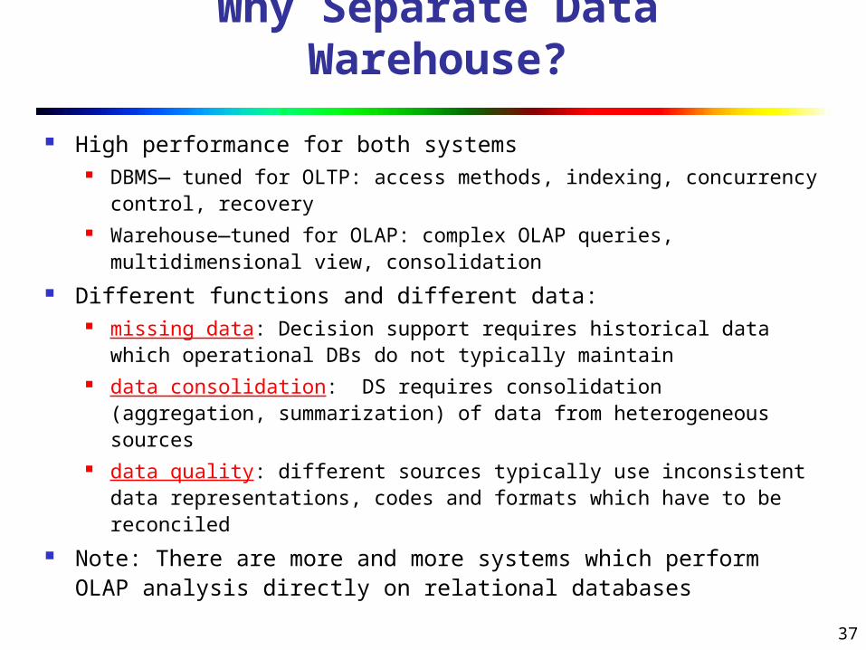
Why Separate Data Warehouse?

High performance for both systems DBMS— tuned for OLTP: access methods, indexing, concurrency

control, recovery Warehouse—tuned for OLAP: complex OLAP queries,

multidimensional view, consolidation Different functions and different data:

missing data: Decision support requires historical data which operational DBs do not typically maintain

data consolidation: DS requires consolidation (aggregation, summarization) of data from heterogeneous sources

data quality: different sources typically use inconsistent data representations, codes and formats which have to be reconciled

Note: There are more and more systems which perform OLAP analysis directly on relational databases

38

From Tables and Spreadsheets to Data Cubes

A data warehouse is based on a multidimensional data

model which views data in the form of a data cube

A data cube, such as sales, allows data to be modeled and

viewed in multiple dimensions Dimension tables, such as item (item_name, brand, type), or

time(day, week, month, quarter, year)

Fact table contains measures (such as dollars_sold) and keys to

each of the related dimension tables

In data warehousing literature, an n-D base cube is called a

base cuboid. The top most 0-D cuboid, which holds the

highest-level of summarization, is called the apex cuboid.

The lattice of cuboids forms a data cube.

39

Chapter 3: Data Generalization, Data Warehousing, and On-line Analytical

Processing

Data generalization and concept description

Data warehouse: Basic concept

Data warehouse modeling: Data cube and OLAP

Data warehouse architecture

Data warehouse implementation

From data warehousing to data mining

40

Cube: A Lattice of Cuboids

time,item

time,item,location

time, item, location, supplier

all

time item location supplier

time,location

time,supplier

item,location

item,supplier

location,supplier

time,item,supplier

time,location,supplier

item,location,supplier

0-D(apex) cuboid

1-D cuboids

2-D cuboids

3-D cuboids

4-D(base) cuboid

41

Conceptual Modeling of Data Warehouses

Modeling data warehouses: dimensions &

measures Star schema: A fact table in the middle connected to a set

of dimension tables Snowflake schema: A refinement of star schema where

some dimensional hierarchy is normalized into a set of

smaller dimension tables, forming a shape similar to

snowflake Fact constellations: Multiple fact tables share dimension

tables, viewed as a collection of stars, therefore called

galaxy schema or fact constellation

42

Example of Star Schema

time_keydayday_of_the_weekmonthquarteryear

time

location_keystreetcitystate_or_provincecountry

location

Sales Fact Table

time_key

item_key

branch_key

location_key

units_sold

dollars_sold

avg_sales

Measures

item_keyitem_namebrandtypesupplier_type

item

branch_keybranch_namebranch_type

branch

43

Example of Snowflake Schema


time

location_keystreetcity_key

location

Sales Fact Table

time_key

item_key

branch_key

location_key

units_sold

dollars_sold

avg_sales

Measures

item_keyitem_namebrandtypesupplier_key

item


branch

supplier_keysupplier_type

supplier

city_keycitystate_or_provincecountry

city

44

Example of Fact Constellation


time

location_keystreetcityprovince_or_statecountry

location

Sales Fact Table

time_key

item_key

branch_key

location_key

units_sold

dollars_sold

avg_sales

Measures

item_keyitem_namebrandtypesupplier_type

item


branch

Shipping Fact Table

time_key

item_key

shipper_key

from_location

to_location

dollars_cost

units_shipped

shipper_keyshipper_namelocation_keyshipper_type

shipper

45

Cube Definition Syntax (BNF) in DMQL

Cube Definition (Fact Table)define cube <cube_name> [<dimension_list>]:

<measure_list> Dimension Definition (Dimension Table)

define dimension <dimension_name> as (<attribute_or_subdimension_list>)

Special Case (Shared Dimension Tables) First time as “cube definition” define dimension <dimension_name> as

<dimension_name_first_time> in cube <cube_name_first_time>

46

Defining Star Schema in DMQL

define cube sales_star [time, item, branch, location]:dollars_sold = sum(sales_in_dollars), avg_sales

= avg(sales_in_dollars), units_sold = count(*)define dimension time as (time_key, day,

day_of_week, month, quarter, year)define dimension item as (item_key, item_name,

brand, type, supplier_type)define dimension branch as (branch_key,

branch_name, branch_type)define dimension location as (location_key, street,

city, province_or_state, country)

47

Defining Snowflake Schema in DMQL

define cube sales_snowflake [time, item, branch, location]:

dollars_sold = sum(sales_in_dollars), avg_sales = avg(sales_in_dollars), units_sold = count(*)

define dimension time as (time_key, day, day_of_week, month, quarter, year)

define dimension item as (item_key, item_name, brand, type, supplier(supplier_key, supplier_type))

define dimension branch as (branch_key, branch_name, branch_type)

define dimension location as (location_key, street, city(city_key, province_or_state, country))

48

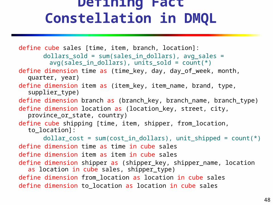
Defining Fact Constellation in DMQL

define cube sales [time, item, branch, location]:dollars_sold = sum(sales_in_dollars), avg_sales =

avg(sales_in_dollars), units_sold = count(*)define dimension time as (time_key, day, day_of_week, month,

quarter, year)define dimension item as (item_key, item_name, brand, type,

supplier_type)define dimension branch as (branch_key, branch_name, branch_type)define dimension location as (location_key, street, city,

province_or_state, country)define cube shipping [time, item, shipper, from_location, to_location]:

dollar_cost = sum(cost_in_dollars), unit_shipped = count(*)define dimension time as time in cube salesdefine dimension item as item in cube salesdefine dimension shipper as (shipper_key, shipper_name, location as

location in cube sales, shipper_type)define dimension from_location as location in cube salesdefine dimension to_location as location in cube sales

49

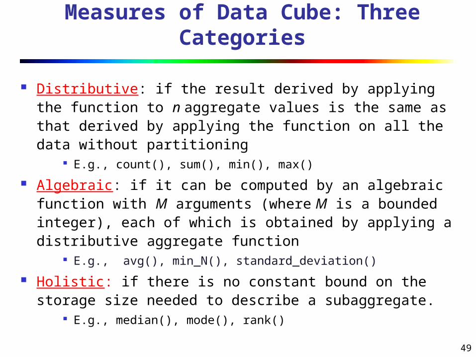
Measures of Data Cube: Three Categories

Distributive: if the result derived by applying the function to n aggregate values is the same as that derived by applying the function on all the data without partitioning

E.g., count(), sum(), min(), max()

Algebraic: if it can be computed by an algebraic function with M arguments (where M is a bounded integer), each of which is obtained by applying a distributive aggregate function

E.g., avg(), min_N(), standard_deviation()

Holistic: if there is no constant bound on the storage size needed to describe a subaggregate.

E.g., median(), mode(), rank()

50

A Concept Hierarchy: Dimension (location)

all

Europe North_America

MexicoCanadaSpainGermany

Vancouver

M. WindL. Chan

...

......

... ...

...

all

region

office

country

TorontoFrankfurtcity

51

Multidimensional Data

Sales volume as a function of product, month, and region

Pro

duct

Regio

n

Month

Dimensions: Product, Location, TimeHierarchical summarization paths

Industry Region Year

Category Country Quarter

Product City Month Week

Office Day

52

A Sample Data Cube

Total annual salesof TV in U.S.A.Date

Produ

ct

Cou

ntr

ysum

sum TV

VCRPC

1Qtr 2Qtr 3Qtr 4Qtr

U.S.A

Canada

Mexico

sum

53

Cuboids Corresponding to the Cube

all

product date country

product,date product,country date, country

product, date, country

0-D(apex) cuboid

1-D cuboids

2-D cuboids

3-D(base) cuboid

54

Typical OLAP Operations

Roll up (drill-up): summarize data by climbing up hierarchy or by dimension reduction

Drill down (roll down): reverse of roll-up from higher level summary to lower level summary or

detailed data, or introducing new dimensions Slice and dice: project and select Pivot (rotate):

reorient the cube, visualization, 3D to series of 2D planes Other operations

drill across: involving (across) more than one fact table drill through: through the bottom level of the cube to its

back-end relational tables (using SQL)

55

Fig. 3.10 Typical OLAP Operations

56

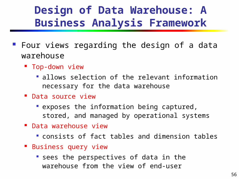
Design of Data Warehouse: A Business Analysis Framework

Four views regarding the design of a data warehouse Top-down view

allows selection of the relevant information necessary for the data warehouse

Data source view exposes the information being captured, stored, and

managed by operational systems Data warehouse view

consists of fact tables and dimension tables Business query view

sees the perspectives of data in the warehouse from the view of end-user

57

Data Warehouse Design Process

Top-down, bottom-up approaches or a combination of both Top-down: Starts with overall design and planning (mature) Bottom-up: Starts with experiments and prototypes (rapid)

From software engineering point of view Waterfall: structured and systematic analysis at each step before

proceeding to the next Spiral: rapid generation of increasingly functional systems, short

turn around time, quick turn around Typical data warehouse design process

Choose a business process to model, e.g., orders, invoices, etc. Choose the grain (atomic level of data) of the business process Choose the dimensions that will apply to each fact table record Choose the measure that will populate each fact table record

58

Data Warehouse: A Multi-Tiered ArchitectureData Warehouse: A Multi-Tiered Architecture

DataWarehouse

ExtractTransformLoadRefresh

OLAP Engine

AnalysisQueryReportsData mining

Monitor&

IntegratorMetadata

Data Sources Front-End Tools

Serve

Data Marts

Operational DBs

Othersources

Data Storage

OLAP Server

59

Three Data Warehouse Models

Enterprise warehouse collects all of the information about subjects spanning the

entire organization Data Mart

a subset of corporate-wide data that is of value to a specific groups of users. Its scope is confined to specific, selected groups, such as marketing data mart

Independent vs. dependent (directly from warehouse) data mart

Virtual warehouse A set of views over operational databases Only some of the possible summary views may be

materialized

60

Data Warehouse Development: A

Recommended Approach

Define a high-level corporate data model

Data Mart

Data Mart

Distributed Data Marts

Multi-Tier Data Warehouse

Enterprise Data Warehouse

Model refinementModel refinement

61

Data Warehouse Back-End Tools and Utilities

Data extraction get data from multiple, heterogeneous, and external

sources Data cleaning

detect errors in the data and rectify them when possible Data transformation

convert data from legacy or host format to warehouse format

Load sort, summarize, consolidate, compute views, check

integrity, and build indicies and partitions Refresh

propagate the updates from the data sources to the warehouse

62

Metadata Repository

Meta data is the data defining warehouse objects. It stores: Description of the structure of the data warehouse

schema, view, dimensions, hierarchies, derived data defn, data mart locations and contents

Operational meta-data data lineage (history of migrated data and transformation path),

currency of data (active, archived, or purged), monitoring information (warehouse usage statistics, error reports, audit trails)

The algorithms used for summarization The mapping from operational environment to the data

warehouse Data related to system performance

warehouse schema, view and derived data definitions Business data

business terms and definitions, ownership of data, charging policies

63

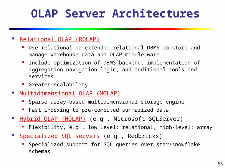
OLAP Server Architectures

Relational OLAP (ROLAP) Use relational or extended-relational DBMS to store and manage

warehouse data and OLAP middle ware Include optimization of DBMS backend, implementation of

aggregation navigation logic, and additional tools and services Greater scalability

Multidimensional OLAP (MOLAP) Sparse array-based multidimensional storage engine Fast indexing to pre-computed summarized data

Hybrid OLAP (HOLAP) (e.g., Microsoft SQLServer) Flexibility, e.g., low level: relational, high-level: array

Specialized SQL servers (e.g., Redbricks) Specialized support for SQL queries over star/snowflake

schemas

64

Efficient Data Cube Computation

Data cube can be viewed as a lattice of cuboids The bottom-most cuboid is the base cuboid The top-most cuboid (apex) contains only one cell How many cuboids in an n-dimensional cube with L

levels?

Materialization of data cube Materialize every (cuboid) (full materialization), none (no

materialization), or some (partial materialization) Selection of which cuboids to materialize

Based on size, sharing, access frequency, etc.

)11(

n

i iLT

65

Data warehouse Implementation

Efficient Cube Computation

Efficient Indexing

Efficient Processing of OLAP Queries

66

Cube Operation

Cube definition and computation in DMQL

define cube sales[item, city, year]: sum(sales_in_dollars)

compute cube sales Transform it into a SQL-like language (with a new

operator cube by, introduced by Gray et al.’96)

SELECT item, city, year, SUM (amount)

FROM SALES

CUBE BY item, city, year Need compute the following Group-Bys

(date, product, customer),(date,product),(date, customer), (product,

customer),(date), (product), (customer)()

(item)(city)

()

(year)

(city, item) (city, year) (item, year)

(city, item, year)

67

Multi-Way Array Multi-Way Array AggregationAggregation

Array-based “bottom-up” algorithm

Using multi-dimensional chunks No direct tuple comparisons Simultaneous aggregation on

multiple dimensions Intermediate aggregate values

are re-used for computing ancestor cuboids

Cannot do Apriori pruning: No iceberg optimization

a ll

A B

A B

A B C

A C B C

C

68

Multi-way Array Aggregation for Cube Computation (MOLAP)

Partition arrays into chunks (a small subcube which fits in memory). Compressed sparse array addressing: (chunk_id, offset) Compute aggregates in “multiway” by visiting cube cells in the order

which minimizes the # of times to visit each cell, and reduces memory access and storage cost.

What is the best traversing order to do multi-way aggregation?

A

B

29 30 31 32

1 2 3 4

5

9

13 14 15 16

6463626148474645

a1a0

c3c2

c1c 0

b3

b2

b1

b0

a2 a3

C

B

4428 56

4024 52

3620

60

69

Multi-way Array Aggregation for Cube

Computation

A

B

29 30 31 32

1 2 3 4

5

9

13 14 15 16

6463626148474645

a1a0

c3c2

c1c 0

b3

b2

b1

b0

a2 a3

C

4428 56

4024 52

3620

60

B

70

Multi-way Array Aggregation for Cube

Computation

A

B

29 30 31 32

1 2 3 4

5

9

13 14 15 16

6463626148474645

a1a0

c3c2

c1c 0

b3

b2

b1

b0

a2 a3

C

4428 56

4024 52

3620

60

B

71

Multi-Way Array Aggregation for Cube Computation (Cont.)

Method: the planes should be sorted and computed according to their size in ascending order Idea: keep the smallest plane in the main memory, fetch

and compute only one chunk at a time for the largest plane

Limitation of the method: computing well only for a small number of dimensions If there are a large number of dimensions, “top-down”

computation and iceberg cube computation methods can be explored

72

Indexing OLAP Data: Bitmap Index

Index on a particular column Each value in the column has a bit vector: bit-op is fast The length of the bit vector: # of records in the base table The i-th bit is set if the i-th row of the base table has the

value for the indexed column not suitable for high cardinality domains

Cust Region TypeC1 Asia RetailC2 Europe DealerC3 Asia DealerC4 America RetailC5 Europe Dealer

RecID Retail Dealer1 1 02 0 13 0 14 1 05 0 1

RecID Asia Europe America1 1 0 02 0 1 03 1 0 04 0 0 15 0 1 0

Base table Index on Region Index on Type

73

Indexing OLAP Data: Join Indices

Join index: JI(R-id, S-id) where R (R-id, …) S (S-id, …)

Traditional indices map the values to a list of record ids It materializes relational join in JI file and

speeds up relational join In data warehouses, join index relates the

values of the dimensions of a start schema to rows in the fact table. E.g. fact table: Sales and two dimensions

city and product A join index on city maintains for

each distinct city a list of R-IDs of the tuples recording the Sales in the city

Join indices can span multiple dimensions

74

Efficient Processing OLAP Queries

Determine which operations should be performed on the available cuboids

Transform drill, roll, etc. into corresponding SQL and/or OLAP operations, e.g.,

dice = selection + projection

Determine which materialized cuboid(s) should be selected for OLAP op.

Let the query to be processed be on {brand, province_or_state} with the

condition “year = 2004”, and there are 4 materialized cuboids available:

1) {year, item_name, city}

2) {year, brand, country}

3) {year, brand, province_or_state}

4) {item_name, province_or_state} where year = 2004

Which should be selected to process the query?

Explore indexing structures and compressed vs. dense array structs in

MOLAP

75

Data Warehouse Usage

Three kinds of data warehouse applications Information processing

supports querying, basic statistical analysis, and reporting using crosstabs, tables, charts and graphs

Analytical processing

multidimensional analysis of data warehouse data supports basic OLAP operations, slice-dice, drilling,

pivoting Data mining

knowledge discovery from hidden patterns supports associations, constructing analytical models,

performing classification and prediction, and presenting the mining results using visualization tools

76

From On-Line Analytical Processing (OLAP)

to On Line Analytical Mining (OLAM) Why online analytical mining?

High quality of data in data warehouses DW contains integrated, consistent, cleaned

data Available information processing structure surrounding

data warehouses ODBC, OLEDB, Web accessing, service

facilities, reporting and OLAP tools OLAP-based exploratory data analysis

Mining with drilling, dicing, pivoting, etc. On-line selection of data mining functions

Integration and swapping of multiple mining functions, algorithms, and tasks

77

An OLAM System Architecture

Data Warehouse

Meta Data

MDDB

OLAMEngine

OLAPEngine

User GUI API

Data Cube API

Database API

Data cleaning

Data integration

Layer3

OLAP/OLAM

Layer2

MDDB

Layer1

Data Repository

Layer4

User Interface

Filtering&Integration Filtering

Databases

Mining query Mining result

78

UNIT II- Data Preprocessing

Data cleaning

Data integration and transformation

Data reduction

Summary

79

Major Tasks in Data Preprocessing

Data cleaning Fill in missing values, smooth noisy data, identify or

remove outliers, and resolve inconsistencies Data integration

Integration of multiple databases, data cubes, or files Data transformation

Normalization and aggregation Data reduction

Obtains reduced representation in volume but produces the same or similar analytical results

Data discretization: part of data reduction, of particular importance for numerical data

80

Data Cleaning

No quality data, no quality mining results! Quality decisions must be based on quality data

e.g., duplicate or missing data may cause incorrect or even misleading statistics

“Data cleaning is the number one problem in data warehousing”—DCI survey

Data extraction, cleaning, and transformation comprises the majority of the work of building a data warehouse

Data cleaning tasks Fill in missing values Identify outliers and smooth out noisy data Correct inconsistent data Resolve redundancy caused by data integration

81

Data in the Real World Is Dirty

incomplete: lacking attribute values, lacking certain attributes of interest, or containing only aggregate data e.g., occupation=“ ” (missing data)

noisy: containing noise, errors, or outliers e.g., Salary=“−10” (an error)

inconsistent: containing discrepancies in codes or names, e.g., Age=“42” Birthday=“03/07/1997” Was rating “1,2,3”, now rating “A, B, C” discrepancy between duplicate records

82

Why Is Data Dirty?

Incomplete data may come from “Not applicable” data value when collected Different considerations between the time when the data was

collected and when it is analyzed. Human/hardware/software problems

Noisy data (incorrect values) may come from Faulty data collection instruments Human or computer error at data entry Errors in data transmission

Inconsistent data may come from Different data sources Functional dependency violation (e.g., modify some linked data)

Duplicate records also need data cleaning

83

Multi-Dimensional Measure of Data Quality

A well-accepted multidimensional view: Accuracy Completeness Consistency Timeliness Believability Value added Interpretability Accessibility

Broad categories: Intrinsic, contextual, representational, and accessibility

84

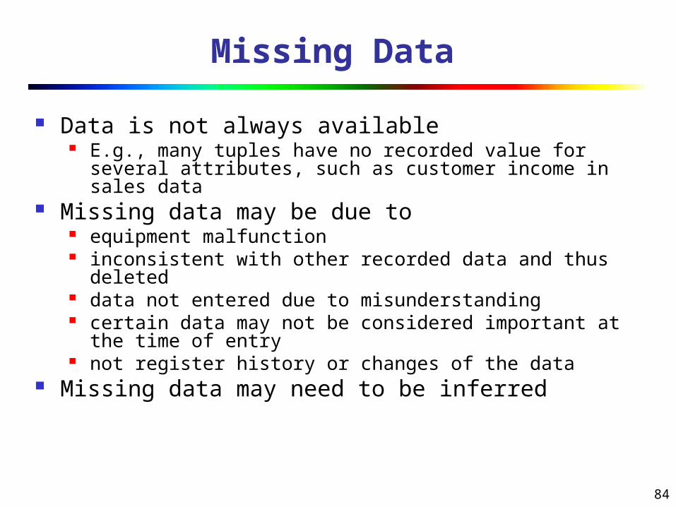
Missing Data

Data is not always available E.g., many tuples have no recorded value for several

attributes, such as customer income in sales data Missing data may be due to

equipment malfunction inconsistent with other recorded data and thus deleted data not entered due to misunderstanding certain data may not be considered important at the time

of entry not register history or changes of the data

Missing data may need to be inferred

85

How to Handle Missing Data?

Ignore the tuple: usually done when class label is missing (when doing classification)—not effective when the % of missing values per attribute varies considerably

Fill in the missing value manually: tedious + infeasible? Fill in it automatically with

a global constant : e.g., “unknown”, a new class?! the attribute mean the attribute mean for all samples belonging to the same class:

smarter the most probable value: inference-based such as Bayesian

formula or decision tree

86

Noisy Data

Noise: random error or variance in a measured variable

Incorrect attribute values may due to faulty data collection instruments data entry problems data transmission problems technology limitation inconsistency in naming convention

Other data problems which requires data cleaning duplicate records incomplete data inconsistent data

87

How to Handle Noisy Data?

Binning first sort data and partition into (equal-frequency) bins then one can smooth by bin means, smooth by bin

median, smooth by bin boundaries, etc. Regression

smooth by fitting the data into regression functions Clustering

detect and remove outliers Combined computer and human inspection

detect suspicious values and check by human (e.g., deal with possible outliers)

88

Simple Discretization Methods: Binning

Equal-width (distance) partitioning Divides the range into N intervals of equal size: uniform grid

if A and B are the lowest and highest values of the attribute, the

width of intervals will be: W = (B –A)/N.

The most straightforward, but outliers may dominate

presentation

Skewed data is not handled well

Equal-depth (frequency) partitioning Divides the range into N intervals, each containing

approximately same number of samples

Good data scaling

Managing categorical attributes can be tricky

89

Binning Methods for Data Smoothing

Sorted data for price (in dollars): 4, 8, 9, 15, 21, 21, 24, 25, 26, 28, 29, 34

* Partition into equal-frequency (equi-depth) bins: - Bin 1: 4, 8, 9, 15 - Bin 2: 21, 21, 24, 25 - Bin 3: 26, 28, 29, 34* Smoothing by bin means: - Bin 1: 9, 9, 9, 9 - Bin 2: 23, 23, 23, 23 - Bin 3: 29, 29, 29, 29* Smoothing by bin boundaries: - Bin 1: 4, 4, 4, 15 - Bin 2: 21, 21, 25, 25 - Bin 3: 26, 26, 26, 34

90

Regression

x

y

y = x + 1

X1

Y1

Y1’

91

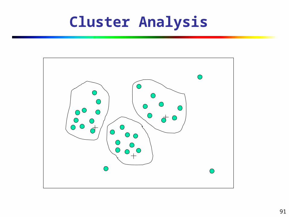
Cluster Analysis

92

Data Cleaning as a Process Data discrepancy detection

Use metadata (e.g., domain, range, dependency, distribution) Check field overloading Check uniqueness rule, consecutive rule and null rule Use commercial tools

Data scrubbing: use simple domain knowledge (e.g., postal code, spell-check) to detect errors and make corrections

Data auditing: by analyzing data to discover rules and relationship to detect violators (e.g., correlation and clustering to find outliers)

Data migration and integration Data migration tools: allow transformations to be specified ETL (Extraction/Transformation/Loading) tools: allow users to

specify transformations through a graphical user interface Integration of the two processes

Iterative and interactive (e.g., Potter’s Wheels)

93

Data Integration

Data integration: Combines data from multiple sources into a coherent store

Schema integration: e.g., A.cust-id B.cust-# Integrate metadata from different sources

Entity identification problem: Identify real world entities from multiple data sources, e.g.,

Bill Clinton = William Clinton Detecting and resolving data value conflicts

For the same real world entity, attribute values from different sources are different

Possible reasons: different representations, different scales, e.g., metric vs. British units

94

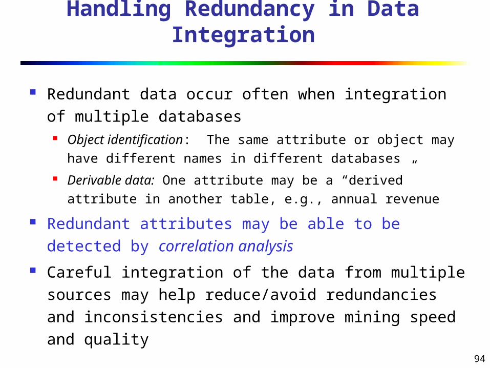
Handling Redundancy in Data Integration

Redundant data occur often when integration of multiple databases Object identification: The same attribute or object may

have different names in different databases Derivable data: One attribute may be a “derived” attribute

in another table, e.g., annual revenue

Redundant attributes may be able to be detected by correlation analysis

Careful integration of the data from multiple sources may help reduce/avoid redundancies and inconsistencies and improve mining speed and quality

95

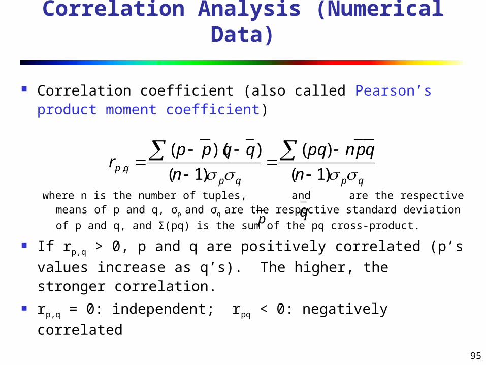
Correlation Analysis (Numerical Data)

Correlation coefficient (also called Pearson’s product moment coefficient)

where n is the number of tuples, and are the respective means of p and q, σp and σq are the respective standard deviation

of p and q, and Σ(pq) is the sum of the pq cross-product.

If rp,q > 0, p and q are positively correlated (p’s

values increase as q’s). The higher, the stronger correlation.

rp,q = 0: independent; rpq < 0: negatively correlated

qpqpqp n

qpnpq

n

qqppr

)1(

)(

)1(

))((,

p q

96

Correlation (viewed as linear relationship)

Correlation measures the linear relationship between objects

To compute correlation, we standardize data objects, p and q, and then take their dot product

)(/))(( pstdpmeanpp kk

)(/))(( qstdqmeanqq kk

qpqpncorrelatio ),(

97

Data Transformation A function that maps the entire set of values of a

given attribute to a new set of replacement values s.t. each old value can be identified with one of the new values

Methods Smoothing: Remove noise from data Aggregation: Summarization, data cube construction Generalization: Concept hierarchy climbing Normalization: Scaled to fall within a small, specified range

min-max normalization z-score normalization normalization by decimal scaling

Attribute/feature construction New attributes constructed from the given

ones

98

Data Transformation: Normalization

Min-max normalization: to [new_minA, new_maxA]

Ex. Let income range $12,000 to $98,000 normalized to [0.0, 1.0]. Then $73,000 is mapped to

Z-score normalization (μ: mean, σ: standard deviation):

Ex. Let μ = 54,000, σ = 16,000. Then

Normalization by decimal scaling

716.00)00.1(000,12000,98

000,12600,73

AAA

AA

A

minnewminnewmaxnewminmax

minvv _)__('

A

Avv

'

j

vv

10' Where j is the smallest integer such that Max(|ν’|) < 1

225.1000,16

000,54600,73

99

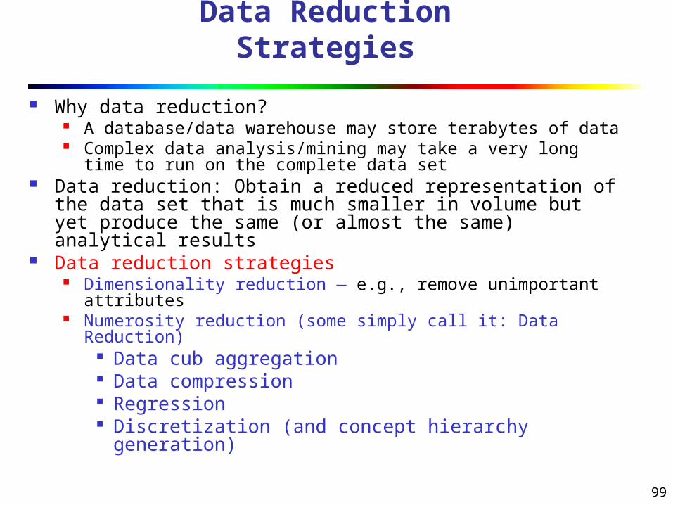
Data Reduction Strategies

Why data reduction? A database/data warehouse may store terabytes of data Complex data analysis/mining may take a very long time to

run on the complete data set Data reduction: Obtain a reduced representation of the

data set that is much smaller in volume but yet produce the same (or almost the same) analytical results

Data reduction strategies Dimensionality reduction — e.g., remove unimportant

attributes Numerosity reduction (some simply call it: Data Reduction)

Data cub aggregation Data compression Regression Discretization (and concept hierarchy generation)

100

Dimensionality Reduction Curse of dimensionality

When dimensionality increases, data becomes increasingly sparse

Density and distance between points, which is critical to clustering, outlier analysis, becomes less meaningful

The possible combinations of subspaces will grow exponentially Dimensionality reduction

Avoid the curse of dimensionality Help eliminate irrelevant features and reduce noise Reduce time and space required in data mining Allow easier visualization

Dimensionality reduction techniques Principal component analysis Singular value decomposition Supervised and nonlinear techniques (e.g., feature selection)

101

x2

x1

e

Dimensionality Reduction: Principal Component Analysis (PCA)

Find a projection that captures the largest amount of variation in data

Find the eigenvectors of the covariance matrix, and these eigenvectors define the new space

102

Given N data vectors from n-dimensions, find k ≤ n orthogonal vectors (principal components) that can be best used to represent data Normalize input data: Each attribute falls within the same range Compute k orthonormal (unit) vectors, i.e., principal components Each input data (vector) is a linear combination of the k principal

component vectors The principal components are sorted in order of decreasing

“significance” or strength Since the components are sorted, the size of the data can be

reduced by eliminating the weak components, i.e., those with low variance (i.e., using the strongest principal components, it is possible to reconstruct a good approximation of the original data)

Works for numeric data only

Principal Component Analysis (Steps)

103

Feature Subset Selection

Another way to reduce dimensionality of data Redundant features

duplicate much or all of the information contained in one or more other attributes

E.g., purchase price of a product and the amount of sales tax paid

Irrelevant features contain no information that is useful for the data mining

task at hand E.g., students' ID is often irrelevant to the task of

predicting students' GPA

104

Heuristic Search in Feature Selection

There are 2d possible feature combinations of d features

Typical heuristic feature selection methods: Best single features under the feature independence

assumption: choose by significance tests Best step-wise feature selection:

The best single-feature is picked first Then next best feature condition to the

first, ... Step-wise feature elimination:

Repeatedly eliminate the worst feature Best combined feature selection and elimination Optimal branch and bound:

Use feature elimination and backtracking

105

Feature Creation

Create new attributes that can capture the important information in a data set much more efficiently than the original attributes

Three general methodologies Feature extraction

domain-specific Mapping data to new space (see: data reduction)

E.g., Fourier transformation, wavelet transformation

Feature construction Combining features Data discretization

106

Mapping Data to a New Space

Two Sine Waves Two Sine Waves + Noise Frequency

Fourier transform Wavelet transform

107

Numerosity (Data) Reduction

Reduce data volume by choosing alternative, smaller forms of data representation

Parametric methods (e.g., regression) Assume the data fits some model, estimate model

parameters, store only the parameters, and discard the data (except possible outliers)

Example: Log-linear models—obtain value at a point in m-D space as the product on appropriate marginal subspaces

Non-parametric methods Do not assume models Major families: histograms, clustering, sampling

108

Parametric Data Reduction: Regression and Log-Linear

Models

Linear regression: Data are modeled to fit a

straight line

Often uses the least-square method to fit the line

Multiple regression: allows a response variable Y

to be modeled as a linear function of

multidimensional feature vector

Log-linear model: approximates discrete

multidimensional probability distributions

109

Linear regression: Y = w X + b Two regression coefficients, w and b, specify the line and

are to be estimated by using the data at hand Using the least squares criterion to the known values of

Y1, Y2, …, X1, X2, …. Multiple regression: Y = b0 + b1 X1 + b2 X2.

Many nonlinear functions can be transformed into the above

Log-linear models: The multi-way table of joint probabilities is approximated

by a product of lower-order tables Probability: p(a, b, c, d) = ab acad bcd

Regress Analysis and Log-Linear Models

110

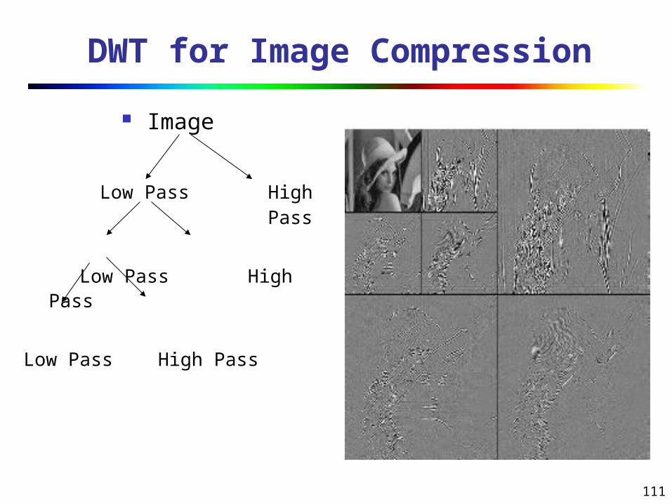
Data Reduction:Wavelet Transformation

Discrete wavelet transform (DWT): linear signal processing, multi-resolutional analysis

Compressed approximation: store only a small fraction of the strongest of the wavelet coefficients

Similar to discrete Fourier transform (DFT), but better lossy compression, localized in space

Method: Length, L, must be an integer power of 2 (padding with 0’s, when

necessary) Each transform has 2 functions: smoothing, difference Applies to pairs of data, resulting in two set of data of length L/2 Applies two functions recursively, until reaches the desired length

Haar2 Daubechie4

111

DWT for Image Compression

Image

Low Pass High Pass

Low Pass High Pass

Low Pass High Pass

112

Data Cube Aggregation

The lowest level of a data cube (base cuboid) The aggregated data for an individual entity of interest E.g., a customer in a phone calling data warehouse

Multiple levels of aggregation in data cubes Further reduce the size of data to deal with

Reference appropriate levels Use the smallest representation which is enough to solve

the task

Queries regarding aggregated information should be answered using data cube, when possible

113

Data Compression

String compression There are extensive theories and well-tuned algorithms Typically lossless But only limited manipulation is possible without expansion

Audio/video compression Typically lossy compression, with progressive refinement Sometimes small fragments of signal can be reconstructed

without reconstructing the whole Time sequence is not audio

Typically short and vary slowly with time

114

Data Compression

Original Data Compressed Data

lossless

Original DataApproximated

lossy

115

Data Reduction: Histograms

Divide data into buckets and store average (sum) for each bucket

Partitioning rules: Equal-width: equal bucket range Equal-frequency (or equal-

depth) V-optimal: with the least

histogram variance (weighted sum of the original values that each bucket represents)

MaxDiff: set bucket boundary between each pair for pairs have the β–1 largest differences

0

5

10

15

20

25

30

35

40

10000 30000 50000 70000 90000

116

Data Reduction Method: Clustering

Partition data set into clusters based on similarity, and store cluster representation (e.g., centroid and diameter) only

Can be very effective if data is clustered but not if data is “smeared”

Can have hierarchical clustering and be stored in multi-dimensional index tree structures

There are many choices of clustering definitions and clustering algorithms

Cluster analysis will be studied in depth in Chapter 7

117

Data Reduction Method: Sampling

Sampling: obtaining a small sample s to represent the whole data set N

Allow a mining algorithm to run in complexity that is potentially sub-linear to the size of the data

Key principle: Choose a representative subset of the data Simple random sampling may have very poor performance

in the presence of skew Develop adaptive sampling methods, e.g., stratified

sampling:

Note: Sampling may not reduce database I/Os (page at a time)

118

Types of Sampling

Simple random sampling There is an equal probability of selecting any particular

item Sampling without replacement

Once an object is selected, it is removed from the population

Sampling with replacement A selected object is not removed from the population

Stratified sampling: Partition the data set, and draw samples from each

partition (proportionally, i.e., approximately the same percentage of the data)

Used in conjunction with skewed data

119

Sampling: With or without Replacement

SRSWOR

(simple random

sample without

replacement)

SRSWR

Raw Data

120

Sampling: Cluster or Stratified Sampling

Raw Data Cluster/Stratified Sample

121

Data Reduction: Discretization

Three types of attributes:

Nominal — values from an unordered set, e.g., color, profession

Ordinal — values from an ordered set, e.g., military or academic

rank

Continuous — real numbers, e.g., integer or real numbers

Discretization:

Divide the range of a continuous attribute into intervals

Some classification algorithms only accept categorical

attributes.

Reduce data size by discretization

Prepare for further analysis

122

Discretization and Concept Hierarchy

Discretization Reduce the number of values for a given continuous attribute by

dividing the range of the attribute into intervals

Interval labels can then be used to replace actual data values

Supervised vs. unsupervised

Split (top-down) vs. merge (bottom-up)

Discretization can be performed recursively on an attribute

Concept hierarchy formation Recursively reduce the data by collecting and replacing low level

concepts (such as numeric values for age) by higher level

concepts (such as young, middle-aged, or senior)

123

Discretization and Concept Hierarchy Generation for Numeric Data

Typical methods: All the methods can be applied recursively

Binning (covered above)

Top-down split, unsupervised,

Histogram analysis (covered above)

Top-down split, unsupervised

Clustering analysis (covered above)

Either top-down split or bottom-up merge, unsupervised

Entropy-based discretization: supervised, top-down split

Interval merging by 2 Analysis: unsupervised, bottom-up merge

Segmentation by natural partitioning: top-down split,

unsupervised

124

Discretization Using Class Labels

Entropy based approach

3 categories for both x and y 5 categories for both x and y

125

Entropy-Based Discretization

Given a set of samples S, if S is partitioned into two intervals S1

and S2 using boundary T, the information gain after partitioning is

Entropy is calculated based on class distribution of the samples in

the set. Given m classes, the entropy of S1 is

where pi is the probability of class i in S1

The boundary that minimizes the entropy function over all possible boundaries is selected as a binary discretization

The process is recursively applied to partitions obtained until some stopping criterion is met

Such a boundary may reduce data size and improve classification accuracy

)(||

||)(

||

||),( 2

21

1SEntropy

SS

SEntropySSTSI

m

iii ppSEntropy

121 )(log)(

126

Discretization Without Using Class Labels

Data Equal interval width

Equal frequency K-means

127

Interval Merge by 2 Analysis

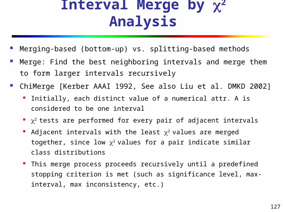
Merging-based (bottom-up) vs. splitting-based methods

Merge: Find the best neighboring intervals and merge them to

form larger intervals recursively

ChiMerge [Kerber AAAI 1992, See also Liu et al. DMKD 2002] Initially, each distinct value of a numerical attr. A is considered to

be one interval

2 tests are performed for every pair of adjacent intervals

Adjacent intervals with the least 2 values are merged together,

since low 2 values for a pair indicate similar class distributions

This merge process proceeds recursively until a predefined

stopping criterion is met (such as significance level, max-interval,

max inconsistency, etc.)

128

Segmentation by Natural Partitioning

A simply 3-4-5 rule can be used to segment

numeric data into relatively uniform, “natural”

intervals. If an interval covers 3, 6, 7 or 9 distinct values at the

most significant digit, partition the range into 3 equi-

width intervals

If it covers 2, 4, or 8 distinct values at the most

significant digit, partition the range into 4 intervals

If it covers 1, 5, or 10 distinct values at the most

significant digit, partition the range into 5 intervals

129

Example of 3-4-5 Rule

(-$400 -$5,000)

(-$400 - 0)

(-$400 - -$300)

(-$300 - -$200)

(-$200 - -$100)

(-$100 - 0)

(0 - $1,000)

(0 - $200)

($200 - $400)

($400 - $600)

($600 - $800) ($800 -

$1,000)

($2,000 - $5, 000)

($2,000 - $3,000)

($3,000 - $4,000)

($4,000 - $5,000)

($1,000 - $2, 000)

($1,000 - $1,200)

($1,200 - $1,400)

($1,400 - $1,600)

($1,600 - $1,800) ($1,800 -

$2,000)

msd=1,000 Low=-$1,000 High=$2,000Step 2:

Step 4:

Step 1: -$351 -$159 profit $1,838 $4,700

Min Low (i.e, 5%-tile) High(i.e, 95%-0 tile) Max

count

(-$1,000 - $2,000)

(-$1,000 - 0) (0 -$ 1,000)

Step 3:

($1,000 - $2,000)

130

Concept Hierarchy Generation for Categorical Data

Specification of a partial/total ordering of attributes explicitly at the schema level by users or experts street < city < state < country

Specification of a hierarchy for a set of values by explicit data grouping {Urbana, Champaign, Chicago} < Illinois

Specification of only a partial set of attributes E.g., only street < city, not others

Automatic generation of hierarchies (or attribute levels) by the analysis of the number of distinct values E.g., for a set of attributes: {street, city, state, country}

131

Automatic Concept Hierarchy Generation

Some hierarchies can be automatically generated based on the analysis of the number of distinct values per attribute in the data set The attribute with the most distinct values is placed at

the lowest level of the hierarchy Exceptions, e.g., weekday, month, quarter, year

country

province_or_ state

city

street

15 distinct values

365 distinct values

3567 distinct values

674,339 distinct values

132

UNIT III: Mining Frequent Patterns, Association and

Correlations

Basic concepts and a road map Efficient and scalable frequent itemset

mining methods Mining various kinds of association rules From association mining to correlation

analysis Constraint-based association mining Summary

133

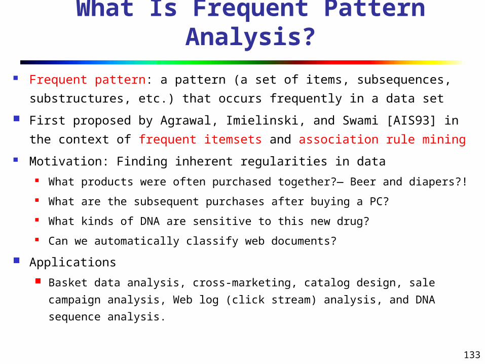
What Is Frequent Pattern Analysis?

Frequent pattern: a pattern (a set of items, subsequences,

substructures, etc.) that occurs frequently in a data set

First proposed by Agrawal, Imielinski, and Swami [AIS93] in the

context of frequent itemsets and association rule mining

Motivation: Finding inherent regularities in data What products were often purchased together?— Beer and diapers?!

What are the subsequent purchases after buying a PC?

What kinds of DNA are sensitive to this new drug?

Can we automatically classify web documents?

Applications

Basket data analysis, cross-marketing, catalog design, sale campaign

analysis, Web log (click stream) analysis, and DNA sequence analysis.

134

Why Is Freq. Pattern Mining Important?

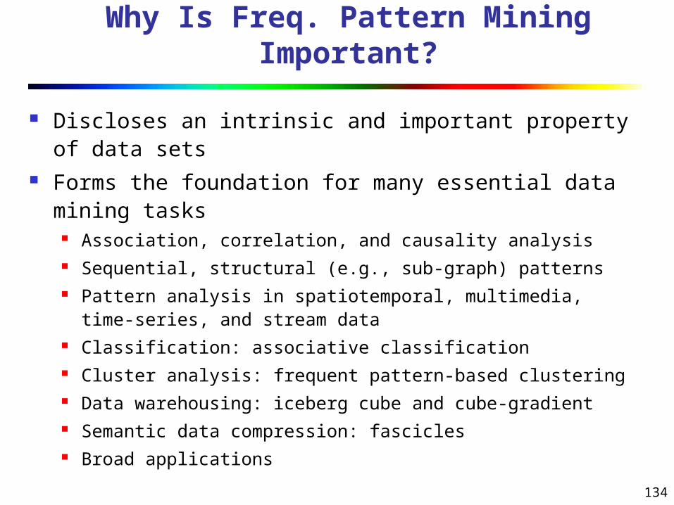
Discloses an intrinsic and important property of data sets

Forms the foundation for many essential data mining tasks Association, correlation, and causality analysis Sequential, structural (e.g., sub-graph) patterns Pattern analysis in spatiotemporal, multimedia, time-

series, and stream data Classification: associative classification Cluster analysis: frequent pattern-based clustering Data warehousing: iceberg cube and cube-gradient Semantic data compression: fascicles Broad applications

135

Basic Concepts: Frequent Patterns and Association Rules

Itemset X = {x1, …, xk} Find all the rules X Y with

minimum support and confidence support, s, probability that a

transaction contains X Y confidence, c, conditional

probability that a transaction having X also contains Y

Let supmin = 50%, confmin = 50%

Freq. Pat.: {A:3, B:3, D:4, E:3, AD:3}Association rules:

A D (60%, 100%)D A (60%, 75%)

Customerbuys diaper

Customerbuys both

Customerbuys beer

Transaction-id Items bought

10 A, B, D

20 A, C, D

30 A, D, E

40 B, E, F

50 B, C, D, E, F

136

Closed Patterns and Max-Patterns

A long pattern contains a combinatorial number of sub-patterns, e.g., {a1, …, a100} contains (100

1) + (1002) + … +

(110000) = 2100 – 1 = 1.27*1030 sub-patterns!

Solution: Mine closed patterns and max-patterns instead An itemset X is closed if X is frequent and there exists no

super-pattern Y כ X, with the same support as X (proposed by Pasquier, et al. @ ICDT’99)

An itemset X is a max-pattern if X is frequent and there exists no frequent super-pattern Y כ X (proposed by Bayardo @ SIGMOD’98)

Closed pattern is a lossless compression of freq. patterns Reducing the # of patterns and rules

137

Closed Patterns and Max-Patterns

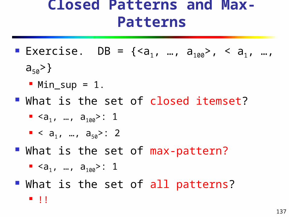
Exercise. DB = {<a1, …, a100>, < a1, …,

a50>} Min_sup = 1.

What is the set of closed itemset? <a1, …, a100>: 1

< a1, …, a50>: 2

What is the set of max-pattern? <a1, …, a100>: 1

What is the set of all patterns? !!

138

Scalable Methods for Mining Frequent Patterns

The downward closure property of frequent patterns Any subset of a frequent itemset must be frequent If {beer, diaper, nuts} is frequent, so is {beer, diaper} i.e., every transaction having {beer, diaper, nuts} also

contains {beer, diaper} Scalable mining methods: Three major approaches

Apriori (Agrawal & Srikant@VLDB’94) Freq. pattern growth (FPgrowth—Han, Pei & Yin

@SIGMOD’00) Vertical data format approach (Charm—Zaki & Hsiao

@SDM’02)

139

Apriori: A Candidate Generation-and-Test Approach

Apriori pruning principle: If there is any itemset which is infrequent, its superset should not be generated/tested! (Agrawal & Srikant @VLDB’94, Mannila, et al. @ KDD’ 94)

Method: Initially, scan DB once to get frequent 1-itemset Generate length (k+1) candidate itemsets from length k

frequent itemsets Test the candidates against DB Terminate when no frequent or candidate set can be

generated

140

The Apriori Algorithm—An Example

Database TDB

1st scan

C1L1

L2

C2 C2

2nd scan

C3 L33rd scan

Tid Items

10 A, C, D

20 B, C, E

30 A, B, C, E

40 B, E

Itemset sup

{A} 2

{B} 3

{C} 3

{D} 1

{E} 3

Itemset sup

{A} 2

{B} 3

{C} 3

{E} 3

Itemset

{A, B}

{A, C}

{A, E}

{B, C}

{B, E}

{C, E}

Itemset sup

{A, B} 1

{A, C} 2

{A, E} 1

{B, C} 2

{B, E} 3

{C, E} 2

Itemset sup

{A, C} 2

{B, C} 2

{B, E} 3

{C, E} 2

Itemset

{B, C, E}

Itemset sup

{B, C, E} 2

Supmin = 2

141

The Apriori Algorithm

Pseudo-code:Ck: Candidate itemset of size kLk : frequent itemset of size k

L1 = {frequent items};for (k = 1; Lk !=; k++) do begin Ck+1 = candidates generated from Lk; for each transaction t in database do

increment the count of all candidates in Ck+1 that are contained in t

Lk+1 = candidates in Ck+1 with min_support endreturn k Lk;

142

Important Details of Apriori

How to generate candidates? Step 1: self-joining Lk

Step 2: pruning How to count supports of candidates? Example of Candidate-generation

L3={abc, abd, acd, ace, bcd}

Self-joining: L3*L3

abcd from abc and abd acde from acd and ace

Pruning: acde is removed because ade is not in L3

C4={abcd}

143

How to Generate Candidates?

Suppose the items in Lk-1 are listed in an order

Step 1: self-joining Lk-1 insert into Ck

select p.item1, p.item2, …, p.itemk-1, q.itemk-1

from Lk-1 p, Lk-1 q

where p.item1=q.item1, …, p.itemk-2=q.itemk-2, p.itemk-1 <

q.itemk-1

Step 2: pruningforall itemsets c in Ck do

forall (k-1)-subsets s of c do

if (s is not in Lk-1) then delete c from Ck

144

How to Count Supports of Candidates?

Why counting supports of candidates a problem? The total number of candidates can be very huge One transaction may contain many candidates

Method: Candidate itemsets are stored in a hash-tree Leaf node of hash-tree contains a list of itemsets and

counts Interior node contains a hash table Subset function: finds all the candidates contained in a

transaction

145

Example: Counting Supports of Candidates

1,4,7

2,5,8

3,6,9Subset function

2 3 45 6 7

1 4 51 3 6

1 2 44 5 7 1 2 5

4 5 81 5 9

3 4 5 3 5 63 5 76 8 9

3 6 73 6 8

Transaction: 1 2 3 5 6

1 + 2 3 5 6

1 2 + 3 5 6

1 3 + 5 6

146

Efficient Implementation of Apriori in SQL

Hard to get good performance out of pure SQL

(SQL-92) based approaches alone

Make use of object-relational extensions like

UDFs, BLOBs, Table functions etc.

Get orders of magnitude improvement

S. Sarawagi, S. Thomas, and R. Agrawal.

Integrating association rule mining with

relational database systems: Alternatives and

implications. In SIGMOD’98

147

Challenges of Frequent Pattern Mining

Challenges Multiple scans of transaction database

Huge number of candidates

Tedious workload of support counting for candidates

Improving Apriori: general ideas Reduce passes of transaction database scans

Shrink number of candidates

Facilitate support counting of candidates

148

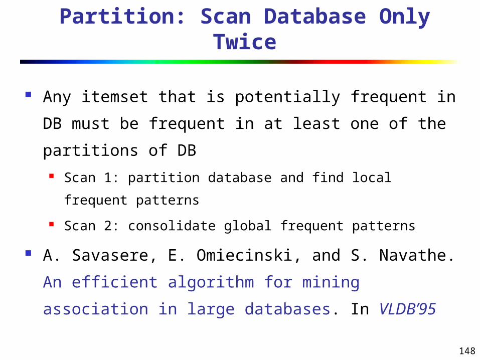
Partition: Scan Database Only Twice

Any itemset that is potentially frequent in DB must

be frequent in at least one of the partitions of DB Scan 1: partition database and find local frequent patterns

Scan 2: consolidate global frequent patterns

A. Savasere, E. Omiecinski, and S. Navathe. An

efficient algorithm for mining association in large

databases. In VLDB’95

149

DHP: Reduce the Number of Candidates

A k-itemset whose corresponding hashing bucket

count is below the threshold cannot be frequent Candidates: a, b, c, d, e

Hash entries: {ab, ad, ae} {bd, be, de} …

Frequent 1-itemset: a, b, d, e

ab is not a candidate 2-itemset if the sum of count of {ab,

ad, ae} is below support threshold

J. Park, M. Chen, and P. Yu. An effective hash-based

algorithm for mining association rules. In

SIGMOD’95

150

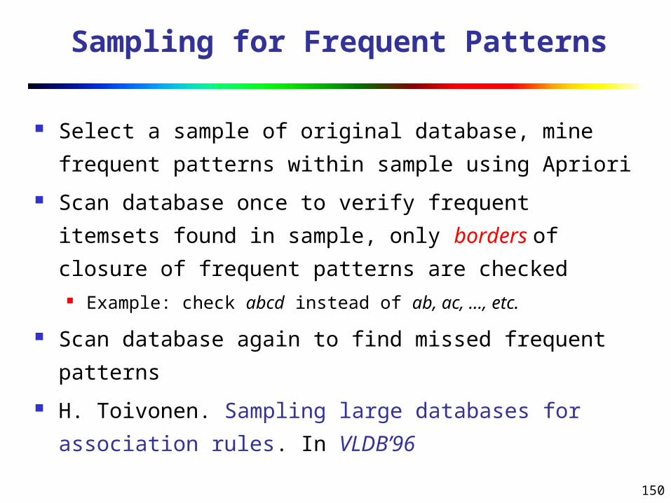
Sampling for Frequent Patterns

Select a sample of original database, mine

frequent patterns within sample using Apriori

Scan database once to verify frequent itemsets

found in sample, only borders of closure of

frequent patterns are checked Example: check abcd instead of ab, ac, …, etc.

Scan database again to find missed frequent

patterns

H. Toivonen. Sampling large databases for

association rules. In VLDB’96

151

DIC: Reduce Number of Scans

ABCD

ABC ABD ACD BCD

AB AC BC AD BD CD

A B C D

{}

Itemset lattice

Once both A and D are determined frequent, the counting of AD begins

Once all length-2 subsets of BCD are determined frequent, the counting of BCD begins

Transactions

1-itemsets2-itemsets

…Apriori

1-itemsets2-items

3-itemsDICS. Brin R. Motwani, J. Ullman, and S. Tsur. Dynamic itemset counting and implication rules for market basket data. In SIGMOD’97

152

Bottleneck of Frequent-pattern Mining

Multiple database scans are costly Mining long patterns needs many passes of

scanning and generates lots of candidates To find frequent itemset i1i2…i100

# of scans: 100 # of Candidates: (100

1) + (1002) + … + (1

10

00

0) =

2100-1 = 1.27*1030 !

Bottleneck: candidate-generation-and-test Can we avoid candidate generation?

153

Mining Frequent Patterns Without Candidate Generation

Grow long patterns from short ones using

local frequent items

“abc” is a frequent pattern

Get all transactions having “abc”: DB|abc

“d” is a local frequent item in DB|abc abcd is a

frequent pattern

154

Construct FP-tree from a Transaction Database

{}

f:4 c:1

b:1

p:1

b:1c:3

a:3

b:1m:2

p:2 m:1

Header Table

Item frequency head f 4c 4a 3b 3m 3p 3

min_support = 3

TID Items bought (ordered) frequent items100 {f, a, c, d, g, i, m, p} {f, c, a, m, p}200 {a, b, c, f, l, m, o} {f, c, a, b, m}300 {b, f, h, j, o, w} {f, b}400 {b, c, k, s, p} {c, b, p}500 {a, f, c, e, l, p, m, n} {f, c, a, m, p}

1. Scan DB once, find frequent 1-itemset (single item pattern)

2. Sort frequent items in frequency descending order, f-list

3. Scan DB again, construct FP-tree F-list=f-c-a-b-m-p

155

Benefits of the FP-tree Structure

Completeness Preserve complete information for frequent pattern mining Never break a long pattern of any transaction

Compactness Reduce irrelevant info—infrequent items are gone Items in frequency descending order: the more frequently

occurring, the more likely to be shared Never be larger than the original database (not count node-

links and the count field) For Connect-4 DB, compression ratio could be over 100

156

Partition Patterns and Databases

Frequent patterns can be partitioned into subsets according to f-list F-list=f-c-a-b-m-p Patterns containing p Patterns having m but no p … Patterns having c but no a nor b, m, p Pattern f

Completeness and non-redundency

157

Find Patterns Having P From P-conditional Database

Starting at the frequent item header table in the FP-tree Traverse the FP-tree by following the link of each frequent

item p Accumulate all of transformed prefix paths of item p to

form p’s conditional pattern base

Conditional pattern bases

item cond. pattern base

c f:3

a fc:3

b fca:1, f:1, c:1

m fca:2, fcab:1

p fcam:2, cb:1

{}

f:4 c:1

b:1

p:1

b:1c:3

a:3

b:1m:2

p:2 m:1

Header Table

Item frequency head f 4c 4a 3b 3m 3p 3

158

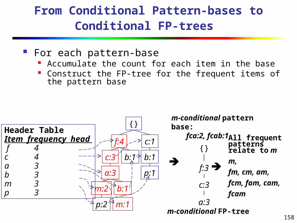
From Conditional Pattern-bases to Conditional FP-trees

For each pattern-base Accumulate the count for each item in the base Construct the FP-tree for the frequent items of the

pattern base

m-conditional pattern base:fca:2, fcab:1

{}

f:3

c:3

a:3m-conditional FP-tree

All frequent patterns relate to m

m,

fm, cm, am,

fcm, fam, cam,

fcam

{}

f:4 c:1

b:1

p:1

b:1c:3

a:3

b:1m:2

p:2 m:1

Header TableItem frequency head f 4c 4a 3b 3m 3p 3

159

Recursion: Mining Each Conditional FP-tree

{}

f:3

c:3

a:3m-conditional FP-tree

Cond. pattern base of “am”: (fc:3)

{}

f:3

c:3am-conditional FP-tree

Cond. pattern base of “cm”: (f:3){}

f:3

cm-conditional FP-tree

Cond. pattern base of “cam”: (f:3)

{}

f:3

cam-conditional FP-tree

160

A Special Case: Single Prefix Path in FP-tree

Suppose a (conditional) FP-tree T has a shared single prefix-path P

Mining can be decomposed into two parts Reduction of the single prefix path into one node Concatenation of the mining results of the two parts

a2:n2

a3:n3

a1:n1

{}

b1:m1C1:k1

C2:k2 C3:k3

b1:m1C1:k1

C2:k2 C3:k3

r1

+a2:n2

a3:n3

a1:n1

{}

r1 =

161

Mining Frequent Patterns With FP-trees

Idea: Frequent pattern growth Recursively grow frequent patterns by pattern and

database partition Method

For each frequent item, construct its conditional pattern-base, and then its conditional FP-tree

Repeat the process on each newly created conditional FP-tree

Until the resulting FP-tree is empty, or it contains only one path—single path will generate all the combinations of its sub-paths, each of which is a frequent pattern

162

Scaling FP-growth by DB Projection

FP-tree cannot fit in memory?—DB projection First partition a database into a set of projected

DBs Then construct and mine FP-tree for each

projected DB Parallel projection vs. Partition projection

techniques Parallel projection is space costly

163

Partition-based Projection

Parallel projection needs a lot of disk space

Partition projection saves it

Tran. DB fcampfcabmfbcbpfcamp

p-proj DB fcamcbfcam

m-proj DB fcabfcafca

b-proj DB fcb…

a-proj DBfc…

c-proj DBf…

f-proj DB …

am-proj DB fcfcfc

cm-proj DB fff

…

164

FP-Growth vs. Apriori: Scalability With the Support Threshold

0

10

20

30

40

50

60

70

80

90

100

0 0.5 1 1.5 2 2.5 3

Support threshold(%)

Ru

n t

ime

(se

c.)

D1 FP-grow th runtime

D1 Apriori runtime

Data set T25I20D10K

165

FP-Growth vs. Tree-Projection: Scalability with the Support Threshold

0

20

40

60

80

100

120

140

0 0.5 1 1.5 2

Support threshold (%)

Ru

nti

me

(sec

.)

D2 FP-growth

D2 TreeProjection

Data set T25I20D100K

166

Why Is FP-Growth the Winner?

Divide-and-conquer: decompose both the mining task and DB according to

the frequent patterns obtained so far leads to focused search of smaller databases

Other factors no candidate generation, no candidate test compressed database: FP-tree structure no repeated scan of entire database basic ops—counting local freq items and building sub FP-

tree, no pattern search and matching

167

Implications of the Methodology

Mining closed frequent itemsets and max-patterns

CLOSET (DMKD’00)

Mining sequential patterns

FreeSpan (KDD’00), PrefixSpan (ICDE’01)

Constraint-based mining of frequent patterns

Convertible constraints (KDD’00, ICDE’01)

Computing iceberg data cubes with complex measures

H-tree and H-cubing algorithm (SIGMOD’01)

168

MaxMiner: Mining Max-patterns

1st scan: find frequent items A, B, C, D, E

2nd scan: find support for AB, AC, AD, AE, ABCDE BC, BD, BE, BCDE CD, CE, CDE, DE,

Since BCDE is a max-pattern, no need to check BCD, BDE, CDE in later scan

R. Bayardo. Efficiently mining long patterns from databases. In SIGMOD’98

Tid Items

10 A,B,C,D,E

20 B,C,D,E,

30 A,C,D,F

Potential max-

patterns

169

Mining Frequent Closed Patterns: CLOSET

Flist: list of all frequent items in support ascending order Flist: d-a-f-e-c

Divide search space Patterns having d Patterns having d but no a, etc.

Find frequent closed pattern recursively Every transaction having d also has cfa cfad is a frequent

closed pattern

J. Pei, J. Han & R. Mao. CLOSET: An Efficient Algorithm for Mining Frequent Closed Itemsets", DMKD'00.

TID Items

10 a, c, d, e, f

20 a, b, e

30 c, e, f

40 a, c, d, f

50 c, e, f

Min_sup=2

170

CLOSET+: Mining Closed Itemsets by Pattern-Growth

Itemset merging: if Y appears in every occurrence of X, then Y is merged with X

Sub-itemset pruning: if Y כ X, and sup(X) = sup(Y), X and all of X’s descendants in the set enumeration tree can be pruned

Hybrid tree projection Bottom-up physical tree-projection Top-down pseudo tree-projection

Item skipping: if a local frequent item has the same support in several header tables at different levels, one can prune it from the header table at higher levels

Efficient subset checking

171

CHARM: Mining by Exploring Vertical Data Format

Vertical format: t(AB) = {T11, T25, …} tid-list: list of trans.-ids containing an itemset

Deriving closed patterns based on vertical intersections t(X) = t(Y): X and Y always happen together t(X) t(Y): transaction having X always has Y

Using diffset to accelerate mining Only keep track of differences of tids t(X) = {T1, T2, T3}, t(XY) = {T1, T3}

Diffset (XY, X) = {T2}

Eclat/MaxEclat (Zaki et al. @KDD’97), VIPER(P. Shenoy et al.@SIGMOD’00), CHARM (Zaki & Hsiao@SDM’02)

172

Further Improvements of Mining Methods

AFOPT (Liu, et al. @ KDD’03) A “push-right” method for mining condensed frequent

pattern (CFP) tree Carpenter (Pan, et al. @ KDD’03)

Mine data sets with small rows but numerous columns Construct a row-enumeration tree for efficient mining

173

Visualization of Association Rules: Plane Graph

174

Visualization of Association Rules: Rule Graph

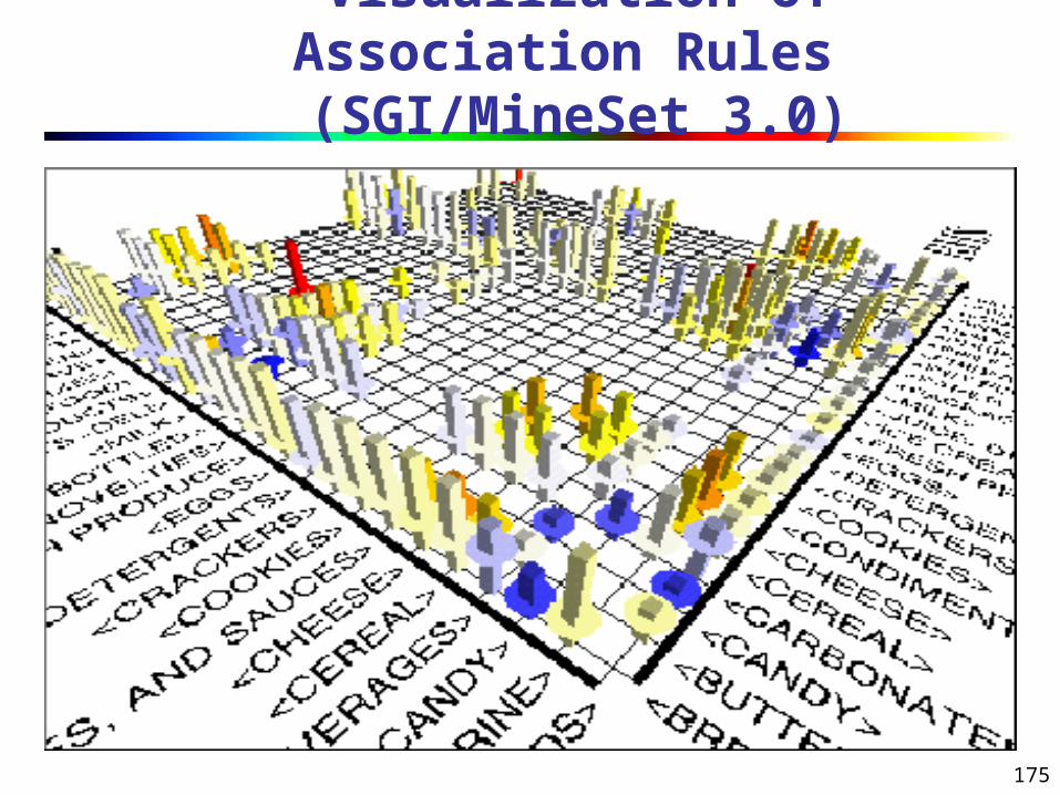
175

Visualization of Association Rules

(SGI/MineSet 3.0)

176

Mining Various Kinds of Association Rules

Mining multilevel association

Miming multidimensional association

Mining quantitative association

Mining interesting correlation patterns

177

Mining Multiple-Level Association Rules

Items often form hierarchies Flexible support settings

Items at the lower level are expected to have lower support

Exploration of shared multi-level mining (Agrawal & Srikant@VLB’95, Han & Fu@VLDB’95)

uniform support

Milk[support = 10%]

2% Milk [support = 6%]

Skim Milk [support = 4%]

Level 1min_sup = 5%

Level 2min_sup = 5%

Level 1min_sup = 5%

Level 2min_sup = 3%

reduced support

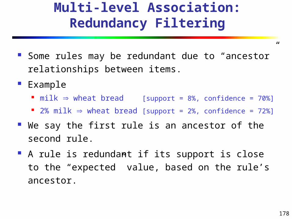
178

Multi-level Association: Redundancy Filtering

Some rules may be redundant due to “ancestor” relationships between items.

Example milk wheat bread [support = 8%, confidence = 70%]

2% milk wheat bread [support = 2%, confidence = 72%]

We say the first rule is an ancestor of the second rule.

A rule is redundant if its support is close to the “expected” value, based on the rule’s ancestor.

179

Mining Multi-Dimensional Association

Single-dimensional rules:buys(X, “milk”) buys(X, “bread”)

Multi-dimensional rules: 2 dimensions or predicates Inter-dimension assoc. rules (no repeated predicates)

age(X,”19-25”) occupation(X,“student”) buys(X, “coke”) hybrid-dimension assoc. rules (repeated predicates)

age(X,”19-25”) buys(X, “popcorn”) buys(X, “coke”)

Categorical Attributes: finite number of possible values, no ordering among values—data cube approach

Quantitative Attributes: numeric, implicit ordering among values—discretization, clustering, and gradient approaches

180

Mining Quantitative Associations

Techniques can be categorized by how numerical attributes, such as age or salary are treated

1. Static discretization based on predefined concept hierarchies (data cube methods)

2. Dynamic discretization based on data distribution (quantitative rules, e.g., Agrawal & Srikant@SIGMOD96)

3. Clustering: Distance-based association (e.g., Yang & Miller@SIGMOD97)

one dimensional clustering then association

4. Deviation: (such as Aumann and Lindell@KDD99)Sex = female => Wage: mean=$7/hr (overall mean = $9)

181

Static Discretization of Quantitative Attributes

Discretized prior to mining using concept hierarchy.

Numeric values are replaced by ranges. In relational database, finding all frequent k-

predicate sets will require k or k+1 table scans. Data cube is well suited for mining. The cells of an n-dimensional

cuboid correspond to the

predicate sets.

Mining from data cubescan be much faster.

(income)(age)

()

(buys)

(age, income) (age,buys) (income,buys)

(age,income,buys)

182

Quantitative Association Rules

age(X,”34-35”) income(X,”30-50K”) buys(X,”high resolution TV”)

Proposed by Lent, Swami and Widom ICDE’97 Numeric attributes are dynamically discretized

Such that the confidence or compactness of the rules mined is maximized

2-D quantitative association rules: Aquan1 Aquan2 Acat

Cluster adjacent association rules to form general rules using a 2-D grid

Example

183

Mining Other Interesting Patterns

Flexible support constraints (Wang et al. @ VLDB’02) Some items (e.g., diamond) may occur rarely but are

valuable Customized supmin specification and application

Top-K closed frequent patterns (Han, et al. @ ICDM’02) Hard to specify supmin, but top-k with lengthmin is more

desirable Dynamically raise supmin in FP-tree construction and

mining, and select most promising path to mine

184

Interestingness Measure: Correlations (Lift)

play basketball eat cereal [40%, 66.7%] is misleading The overall % of students eating cereal is 75% > 66.7%.

play basketball not eat cereal [20%, 33.3%] is more

accurate, although with lower support and confidence

Measure of dependent/correlated events: lift

89.05000/3750*5000/3000

5000/2000),( CBlift

Basketball

Not basketball Sum (row)

Cereal 2000 1750 3750

Not cereal 1000 250 1250

Sum(col.) 3000 2000 5000)()(

)(

BPAP

BAPlift

33.15000/1250*5000/3000

5000/1000),( CBlift

185

Are lift and 2 Good Measures of Correlation?

“Buy walnuts buy milk [1%, 80%]” is misleading if 85% of customers buy milk

Support and confidence are not good to represent correlations

So many interestingness measures? (Tan, Kumar, Sritastava

@KDD’02)

Milk No Milk Sum (row)

Coffee m, c ~m, c c

No Coffee

m, ~c ~m, ~c ~c

Sum(col.)

m ~m

)()(

)(

BPAP

BAPlift

DB m, c ~m, c

m~c ~m~c lift all-conf

coh 2

A1 1000 100 100 10,000 9.26

0.91 0.83 9055

A2 100 1000 1000 100,000

8.44

0.09 0.05 670

A3 1000 100 10000

100,000

9.18

0.09 0.09 8172

A4 1000 1000 1000 1000 1 0.5 0.33 0

)sup(_max_

)sup(_

Xitem

Xconfall

|)(|

)sup(

Xuniverse

Xcoh

186

Which Measures Should Be Used?

lift and 2 are not good measures for correlations in large transactional DBs

all-conf or coherence could be good measures (Omiecinski@TKDE’03)

Both all-conf and coherence have the downward closure property

Efficient algorithms can be derived for mining (Lee et al. @ICDM’03sub)

187

Constraint-based (Query-Directed) Mining

Finding all the patterns in a database autonomously? — unrealistic! The patterns could be too many but not focused!

Data mining should be an interactive process User directs what to be mined using a data mining query

language (or a graphical user interface)

Constraint-based mining User flexibility: provides constraints on what to be mined System optimization: explores such constraints for

efficient mining—constraint-based mining

188

Constraints in Data Mining

Knowledge type constraint: classification, association, etc.

Data constraint — using SQL-like queries find product pairs sold together in stores in Chicago in

Dec.’02 Dimension/level constraint

in relevance to region, price, brand, customer category Rule (or pattern) constraint

small sales (price < $10) triggers big sales (sum > $200) Interestingness constraint

strong rules: min_support 3%, min_confidence 60%

189

Constrained Mining vs. Constraint-Based Search

Constrained mining vs. constraint-based search/reasoning Both are aimed at reducing search space Finding all patterns satisfying constraints vs. finding some

(or one) answer in constraint-based search in AI Constraint-pushing vs. heuristic search It is an interesting research problem on how to integrate

them Constrained mining vs. query processing in DBMS

Database query processing requires to find all Constrained pattern mining shares a similar philosophy as

pushing selections deeply in query processing

190

Anti-Monotonicity in Constraint Pushing

Anti-monotonicity When an intemset S violates the

constraint, so does any of its superset sum(S.Price) v is anti-monotone sum(S.Price) v is not anti-monotone

Example. C: range(S.profit) 15 is anti-monotone Itemset ab violates C So does every superset of ab

TransactionTID

a, b, c, d, f10

b, c, d, f, g, h20

a, c, d, e, f30

c, e, f, g40

TDB (min_sup=2)

Item Profit

a 40

b 0

c -20

d 10

e -30

f 30

g 20

h -10

191

Monotonicity for Constraint Pushing

Monotonicity When an intemset S satisfies the

constraint, so does any of its superset sum(S.Price) v is monotone min(S.Price) v is monotone

Example. C: range(S.profit) 15 Itemset ab satisfies C So does every superset of ab

TransactionTID

a, b, c, d, f10

b, c, d, f, g, h20

a, c, d, e, f30

c, e, f, g40

TDB (min_sup=2)

Item Profit

a 40

b 0

c -20

d 10

e -30

f 30

g 20

h -10

192

Succinctness

Succinctness: Given A1, the set of items satisfying a succinctness

constraint C, then any set S satisfying C is based on A1 ,

i.e., S contains a subset belonging to A1

Idea: Without looking at the transaction database, whether an itemset S satisfies constraint C can be determined based on the selection of items

min(S.Price) v is succinct sum(S.Price) v is not succinct

Optimization: If C is succinct, C is pre-counting pushable

193

The Apriori Algorithm — Example

TID Items100 1 3 4200 2 3 5300 1 2 3 5400 2 5

Database D itemset sup.{1} 2{2} 3{3} 3{4} 1{5} 3

itemset sup.{1} 2{2} 3{3} 3{5} 3

Scan D

C1L1

itemset{1 2}{1 3}{1 5}{2 3}{2 5}{3 5}

itemset sup{1 2} 1{1 3} 2{1 5} 1{2 3} 2{2 5} 3{3 5} 2

itemset sup{1 3} 2{2 3} 2{2 5} 3{3 5} 2

L2

C2 C2

Scan D

C3 L3itemset{2 3 5}

Scan D itemset sup{2 3 5} 2

194

Naïve Algorithm: Apriori + Constraint

TID Items100 1 3 4200 2 3 5300 1 2 3 5400 2 5


itemset sup.{1} 2{2} 3{3} 3{5} 3

Scan D

C1L1

itemset{1 2}{1 3}{1 5}{2 3}{2 5}{3 5}

itemset sup{1 2} 1{1 3} 2{1 5} 1{2 3} 2{2 5} 3{3 5} 2

itemset sup{1 3} 2{2 3} 2{2 5} 3{3 5} 2

L2

C2 C2

Scan D

C3 L3itemset{2 3 5}


Constraint:

Sum{S.price} < 5

195

The Constrained Apriori Algorithm: Push an Anti-

monotone Constraint Deep

TID Items100 1 3 4200 2 3 5300 1 2 3 5400 2 5


itemset sup.{1} 2{2} 3{3} 3{5} 3

Scan D

C1L1

itemset{1 2}{1 3}{1 5}{2 3}{2 5}{3 5}

itemset sup{1 2} 1{1 3} 2{1 5} 1{2 3} 2{2 5} 3{3 5} 2

itemset sup{1 3} 2{2 3} 2{2 5} 3{3 5} 2

L2

C2 C2

Scan D

C3 L3itemset{2 3 5}


Constraint:

Sum{S.price} < 5

196

The Constrained Apriori Algorithm: Push a Succinct

Constraint Deep

TID Items100 1 3 4200 2 3 5300 1 2 3 5400 2 5


itemset sup.{1} 2{2} 3{3} 3{5} 3

Scan D

C1L1

itemset{1 2}{1 3}{1 5}{2 3}{2 5}{3 5}

itemset sup{1 2} 1{1 3} 2{1 5} 1{2 3} 2{2 5} 3{3 5} 2

itemset sup{1 3} 2{2 3} 2{2 5} 3{3 5} 2

L2

C2 C2

Scan D

C3 L3itemset{2 3 5}


Constraint:

min{S.price } <= 1

not immediately to be used

197

Converting “Tough” Constraints

Convert tough constraints into anti-monotone or monotone by properly ordering items

Examine C: avg(S.profit) 25 Order items in value-descending order

<a, f, g, d, b, h, c, e> If an itemset afb violates C

So does afbh, afb* It becomes anti-monotone!

TransactionTID

a, b, c, d, f10

b, c, d, f, g, h20

a, c, d, e, f30

c, e, f, g40

TDB (min_sup=2)

Item Profit

a 40

b 0

c -20

d 10

e -30

f 30

g 20

h -10

198

Strongly Convertible Constraints

avg(X) 25 is convertible anti-monotone w.r.t. item value descending order R: <a, f, g, d, b, h, c, e> If an itemset af violates a constraint C, so does

every itemset with af as prefix, such as afd avg(X) 25 is convertible monotone

w.r.t. item value ascending order R-1: <e, c, h, b, d, g, f, a> If an itemset d satisfies a constraint C, so does

itemsets df and dfa, which having d as a prefix Thus, avg(X) 25 is strongly convertible

Item Profit

a 40

b 0

c -20

d 10

e -30

f 30

g 20

h -10

199

Can Apriori Handle Convertible Constraint?

A convertible, not monotone nor anti-monotone nor succinct constraint cannot be pushed deep into the an Apriori mining algorithm Within the level wise framework, no direct

pruning based on the constraint can be made Itemset df violates constraint C: avg(X)>=25 Since adf satisfies C, Apriori needs df to

assemble adf, df cannot be pruned But it can be pushed into frequent-pattern

growth framework!

Item Value

a 40

b 0

c -20

d 10

e -30

f 30

g 20

h -10

200

Mining With Convertible Constraints

C: avg(X) >= 25, min_sup=2 List items in every transaction in value

descending order R: <a, f, g, d, b, h, c, e> C is convertible anti-monotone w.r.t. R

Scan TDB once remove infrequent items

Item h is dropped Itemsets a and f are good, …

Projection-based mining Imposing an appropriate order on item projection Many tough constraints can be converted into

(anti)-monotone

TransactionTID

a, f, d, b, c10

f, g, d, b, c20

a, f, d, c, e30

f, g, h, c, e40

TDB (min_sup=2)

Item Value

a 40

f 30

g 20

d 10

b 0

h -10

c -20

e -30

201

Handling Multiple Constraints

Different constraints may require different or even conflicting item-ordering

If there exists an order R s.t. both C1 and C2 are

convertible w.r.t. R, then there is no conflict between the two convertible constraints

If there exists conflict on order of items Try to satisfy one constraint first Then using the order for the other constraint to mine

frequent itemsets in the corresponding projected database

202

What Constraints Are Convertible?

Constraint Convertible anti-monotone

Convertible monotone

Strongly convertible

avg(S) , v Yes Yes Yes

median(S) , v Yes Yes Yes

sum(S) v (items could be of any value, v 0) Yes No No

sum(S) v (items could be of any value, v 0) No Yes No

sum(S) v (items could be of any value, v 0) No Yes No

sum(S) v (items could be of any value, v 0) Yes No No

……

203

Constraint-Based Mining—A General Picture

Constraint Antimonotone Monotone Succinct

v S no yes yes

S V no yes yes

S V yes no yes

min(S) v no yes yes

min(S) v yes no yes

max(S) v yes no yes

max(S) v no yes yes

count(S) v yes no weakly

count(S) v no yes weakly

sum(S) v ( a S, a 0 ) yes no no

sum(S) v ( a S, a 0 ) no yes no

range(S) v yes no no

range(S) v no yes no

avg(S) v, { , , } convertible convertible no

support(S) yes no no

support(S) no yes no

204

A Classification of Constraints

Convertibleanti-monotone

Convertiblemonotone

Stronglyconvertible

Inconvertible

Succinct

Antimonotone

Monotone

205

Chapter 6. Classification and Prediction

What is classification? What

is prediction?

Issues regarding

classification and prediction

Classification by decision

tree induction

Bayesian classification

Rule-based classification

Classification by back

propagation

Support Vector Machines

(SVM)

Associative classification

Lazy learners (or learning

from your neighbors)

Other classification methods

Prediction

Accuracy and error measures

Ensemble methods

Model selection

Summary

206

Classification predicts categorical class labels (discrete or nominal) classifies data (constructs a model) based on the training

set and the values (class labels) in a classifying attribute and uses it in classifying new data

Prediction models continuous-valued functions, i.e., predicts

unknown or missing values Typical applications

Credit approval Target marketing Medical diagnosis Fraud detection

Classification vs. Prediction

207

Classification—A Two-Step Process

Model construction: describing a set of predetermined classes Each tuple/sample is assumed to belong to a predefined class,

as determined by the class label attribute The set of tuples used for model construction is training set The model is represented as classification rules, decision

trees, or mathematical formulae Model usage: for classifying future or unknown objects

Estimate accuracy of the model The known label of test sample is compared with the

classified result from the model Accuracy rate is the percentage of test set samples

that are correctly classified by the model Test set is independent of training set, otherwise

over-fitting will occur If the accuracy is acceptable, use the model to classify data

tuples whose class labels are not known

208

Process (1): Model Construction

TrainingData

NAME RANK YEARS TENUREDMike Assistant Prof 3 noMary Assistant Prof 7 yesBill Professor 2 yesJim Associate Prof 7 yesDave Assistant Prof 6 noAnne Associate Prof 3 no

ClassificationAlgorithms

IF rank = ‘professor’OR years > 6THEN tenured = ‘yes’

Classifier(Model)

209

Process (2): Using the Model in Prediction

Classifier

TestingData

NAME RANK YEARS TENUREDTom Assistant Prof 2 noMerlisa Associate Prof 7 noGeorge Professor 5 yesJoseph Assistant Prof 7 yes

Unseen Data

(Jeff, Professor, 4)

Tenured?

210

Supervised vs. Unsupervised Learning

Supervised learning (classification) Supervision: The training data (observations,

measurements, etc.) are accompanied by labels indicating the class of the observations

New data is classified based on the training set

Unsupervised learning (clustering) The class labels of training data is unknown Given a set of measurements, observations, etc. with

the aim of establishing the existence of classes or clusters in the data

211

Issues: Data Preparation

Data cleaning Preprocess data in order to reduce noise and handle

missing values

Relevance analysis (feature selection) Remove the irrelevant or redundant attributes

Data transformation Generalize and/or normalize data

212

Issues: Evaluating Classification Methods

Accuracy classifier accuracy: predicting class label predictor accuracy: guessing value of predicted attributes

Speed time to construct the model (training time) time to use the model (classification/prediction time)

Robustness: handling noise and missing values Scalability: efficiency in disk-resident databases Interpretability

understanding and insight provided by the model Other measures, e.g., goodness of rules, such as

decision tree size or compactness of classification rules

213

Decision Tree Induction: Training Dataset

age income student credit_rating buys_computer<=30 high no fair no<=30 high no excellent no31…40 high no fair yes>40 medium no fair yes>40 low yes fair yes>40 low yes excellent no31…40 low yes excellent yes<=30 medium no fair no<=30 low yes fair yes>40 medium yes fair yes<=30 medium yes excellent yes31…40 medium no excellent yes31…40 high yes fair yes>40 medium no excellent no

This follows an example of Quinlan’s ID3 (Playing Tennis)

214

Output: A Decision Tree for “buys_computer”

age?

overcast

student? credit rating?

<=30 >40

no yes yes

yes

31..40

no

fairexcellentyesno

215

Algorithm for Decision Tree Induction

Basic algorithm (a greedy algorithm) Tree is constructed in a top-down recursive divide-and-conquer

manner At start, all the training examples are at the root Attributes are categorical (if continuous-valued, they are

discretized in advance) Examples are partitioned recursively based on selected

attributes Test attributes are selected on the basis of a heuristic or

statistical measure (e.g., information gain) Conditions for stopping partitioning

All samples for a given node belong to the same class There are no remaining attributes for further partitioning –

majority voting is employed for classifying the leaf There are no samples left

216

Attribute Selection Measure: Information Gain (ID3/C4.5)

Select the attribute with the highest information gain

Let pi be the probability that an arbitrary tuple in D belongs to class Ci, estimated by |Ci, D|/|D|

Expected information (entropy) needed to classify a tuple in D:

Information needed (after using A to split D into v partitions) to classify D:

Information gained by branching on attribute A

)(log)( 21

i

m

ii ppDInfo

)(||

||)(

1j

v

j

jA DI

D

DDInfo

(D)InfoInfo(D)Gain(A) A

217

Attribute Selection: Information Gain

Class P: buys_computer = “yes”

Class N: buys_computer = “no”

means “age <=30” has

5 out of 14 samples, with 2

yes’es and 3 no’s. Hence

Similarly,

age pi ni I(pi, ni)<=30 2 3 0.97131…40 4 0 0>40 3 2 0.971

694.0)2,3(14

5

)0,4(14

4)3,2(

14

5)(

I

IIDInfoage

048.0)_(

151.0)(

029.0)(

ratingcreditGain

studentGain

incomeGain

246.0)()()( DInfoDInfoageGain ageage income student credit_rating buys_computer

<=30 high no fair no<=30 high no excellent no31…40 high no fair yes>40 medium no fair yes>40 low yes fair yes>40 low yes excellent no31…40 low yes excellent yes<=30 medium no fair no<=30 low yes fair yes>40 medium yes fair yes<=30 medium yes excellent yes31…40 medium no excellent yes31…40 high yes fair yes>40 medium no excellent no

)3,2(14

5I

940.0)14

5(log

14

5)

14

9(log

14

9)5,9()( 22 IDInfo

218

Computing Information-Gain for Continuous-Value Attributes

Let attribute A be a continuous-valued attribute Must determine the best split point for A

Sort the value A in increasing order Typically, the midpoint between each pair of adjacent

values is considered as a possible split point

(ai+ai+1)/2 is the midpoint between the values of ai and

ai+1

The point with the minimum expected information requirement for A is selected as the split-point for A

Split: D1 is the set of tuples in D satisfying A ≤ split-point, and D2

is the set of tuples in D satisfying A > split-point

219

Gain Ratio for Attribute Selection (C4.5)

Information gain measure is biased towards attributes with a large number of values

C4.5 (a successor of ID3) uses gain ratio to overcome the problem (normalization to information gain)

GainRatio(A) = Gain(A)/SplitInfo(A)

Ex. gain_ratio(income) = 0.029/0.926 = 0.031

The attribute with the maximum gain ratio is selected as the splitting attribute

)||

||(log

||

||)( 2

1 D

D

D

DDSplitInfo j

v

j

jA

926.0)14

4(log

14

4)

14

6(log

14

6)

14

4(log

14

4)( 222 DSplitInfoA

220

Gini index (CART, IBM IntelligentMiner)

If a data set D contains examples from n classes, gini index, gini(D) is defined as

where pj is the relative frequency of class j in D If a data set D is split on A into two subsets D1 and D2, the

gini index gini(D) is defined as

Reduction in Impurity:

The attribute provides the smallest ginisplit(D) (or the largest

reduction in impurity) is chosen to split the node (need to enumerate all the possible splitting points for each attribute)

n

jp jDgini

1

21)(

)(||||)(

||||)( 2

21

1 DginiDD

DginiDDDginiA

)()()( DginiDginiAginiA

221

Gini index (CART, IBM IntelligentMiner)

Ex. D has 9 tuples in buys_computer = “yes” and 5 in “no”

Suppose the attribute income partitions D into 10 in D1: {low,

medium} and 4 in D2

but gini{medium,high} is 0.30 and thus the best since it is the lowest

All attributes are assumed continuous-valued May need other tools, e.g., clustering, to get the possible split

values Can be modified for categorical attributes

459.014

5

14

91)(

22

Dgini

)(14

4)(

14

10)( 11},{ DGiniDGiniDgini mediumlowincome

222

Comparing Attribute Selection Measures

The three measures, in general, return good results but Information gain:

biased towards multivalued attributes Gain ratio:

tends to prefer unbalanced splits in which one partition is much smaller than the others

Gini index:

biased to multivalued attributes has difficulty when # of classes is large tends to favor tests that result in equal-sized

partitions and purity in both partitions

223

Other Attribute Selection Measures

CHAID: a popular decision tree algorithm, measure based on χ2 test for independence

C-SEP: performs better than info. gain and gini index in certain cases

G-statistics: has a close approximation to χ2 distribution MDL (Minimal Description Length) principle (i.e., the simplest

solution is preferred): The best tree as the one that requires the fewest # of bits to both (1)

encode the tree, and (2) encode the exceptions to the tree

Multivariate splits (partition based on multiple variable combinations) CART: finds multivariate splits based on a linear comb. of attrs.

Which attribute selection measure is the best? Most give good results, none is significantly superior than others

224

Overfitting and Tree Pruning

Overfitting: An induced tree may overfit the training data Too many branches, some may reflect anomalies due to noise or

outliers Poor accuracy for unseen samples

Two approaches to avoid overfitting Prepruning: Halt tree construction early—do not split a node if this

would result in the goodness measure falling below a threshold

Difficult to choose an appropriate threshold Postpruning: Remove branches from a “fully grown” tree—get a

sequence of progressively pruned trees

Use a set of data different from the training data to decide which is the “best pruned tree”

225

Enhancements to Basic Decision Tree Induction

Allow for continuous-valued attributes Dynamically define new discrete-valued attributes that

partition the continuous attribute value into a discrete set of intervals

Handle missing attribute values Assign the most common value of the attribute Assign probability to each of the possible values

Attribute construction Create new attributes based on existing ones that are

sparsely represented This reduces fragmentation, repetition, and replication

226

Classification in Large Databases

Classification—a classical problem extensively studied by statisticians and machine learning researchers

Scalability: Classifying data sets with millions of examples and hundreds of attributes with reasonable speed

Why decision tree induction in data mining? relatively faster learning speed (than other classification

methods) convertible to simple and easy to understand classification

rules can use SQL queries for accessing databases comparable classification accuracy with other methods

227

Scalable Decision Tree Induction Methods

SLIQ (EDBT’96 — Mehta et al.) Builds an index for each attribute and only class list and

the current attribute list reside in memory SPRINT (VLDB’96 — J. Shafer et al.)

Constructs an attribute list data structure PUBLIC (VLDB’98 — Rastogi & Shim)

Integrates tree splitting and tree pruning: stop growing the tree earlier

RainForest (VLDB’98 — Gehrke, Ramakrishnan & Ganti) Builds an AVC-list (attribute, value, class label)

BOAT (PODS’99 — Gehrke, Ganti, Ramakrishnan & Loh) Uses bootstrapping to create several small samples

228

Scalability Framework for RainForest

Separates the scalability aspects from the criteria that

determine the quality of the tree

Builds an AVC-list: AVC (Attribute, Value, Class_label)

AVC-set (of an attribute X ) Projection of training dataset onto the attribute X and class label

where counts of individual class label are aggregated

AVC-group (of a node n ) Set of AVC-sets of all predictor attributes at the node n

229

Rainforest: Training Set and Its AVC Sets

student Buy_Computer

yes no

yes 6 1

no 3 4

Age Buy_Computer

yes no

<=30 3 2

31..40 4 0

>40 3 2

Creditrating

Buy_Computer

yes no

fair 6 2

excellent 3 3

age income studentcredit_ratingbuys_computer<=30 high no fair no<=30 high no excellent no31…40 high no fair yes>40 medium no fair yes>40 low yes fair yes>40 low yes excellent no31…40 low yes excellent yes<=30 medium no fair no<=30 low yes fair yes>40 medium yes fair yes<=30 medium yes excellent yes31…40 medium no excellent yes31…40 high yes fair yes>40 medium no excellent no

AVC-set on incomeAVC-set on Age

AVC-set on Student

Training Examplesincome Buy_Computer

yes no

high 2 2

medium 4 2

low 3 1

AVC-set on credit_rating

230

Data Cube-Based Decision-Tree Induction

Integration of generalization with decision-tree induction (Kamber et al.’97)

Classification at primitive concept levels E.g., precise temperature, humidity, outlook, etc. Low-level concepts, scattered classes, bushy classification-

trees Semantic interpretation problems

Cube-based multi-level classification Relevance analysis at multi-levels Information-gain analysis with dimension + level

231

BOAT (Bootstrapped Optimistic Algorithm for Tree Construction)

Use a statistical technique called bootstrapping to create

several smaller samples (subsets), each fits in memory

Each subset is used to create a tree, resulting in several

trees

These trees are examined and used to construct a new

tree T’ It turns out that T’ is very close to the tree that would be

generated using the whole data set together

Adv: requires only two scans of DB, an incremental alg.

232

Presentation of Classification Results

233

Visualization of a Decision Tree in SGI/MineSet 3.0

234

Interactive Visual Mining by Perception-Based Classification (PBC)

235

Chapter 6. Classification and Prediction

What is classification? What

is prediction?

Issues regarding

classification and prediction

Classification by decision

tree induction

Bayesian classification

Rule-based classification

Classification by back

propagation

Support Vector Machines

(SVM)

Associative classification

Lazy learners (or learning

from your neighbors)

Other classification methods

Prediction

Accuracy and error measures

Ensemble methods

Model selection

Summary

236

Bayesian Classification: Why?

A statistical classifier: performs probabilistic prediction, i.e., predicts class membership probabilities

Foundation: Based on Bayes’ Theorem. Performance: A simple Bayesian classifier, naïve

Bayesian classifier, has comparable performance with decision tree and selected neural network classifiers

Incremental: Each training example can incrementally increase/decrease the probability that a hypothesis is correct — prior knowledge can be combined with observed data

Standard: Even when Bayesian methods are computationally intractable, they can provide a standard of optimal decision making against which other methods can be measured

237

Bayesian Theorem: Basics

Let X be a data sample (“evidence”): class label is unknown

Let H be a hypothesis that X belongs to class C Classification is to determine P(H|X), the probability that

the hypothesis holds given the observed data sample X P(H) (prior probability), the initial probability

E.g., X will buy computer, regardless of age, income, …

P(X): probability that sample data is observed P(X|H) (posteriori probability), the probability of

observing the sample X, given that the hypothesis holds E.g., Given that X will buy computer, the prob. that X is 31..40,

medium income

238

Bayesian Theorem

Given training data X, posteriori probability of a hypothesis H, P(H|X), follows the Bayes theorem

Informally, this can be written as posteriori = likelihood x prior/evidence

Predicts X belongs to C2 iff the probability P(Ci|X) is

the highest among all the P(Ck|X) for all the k classes

Practical difficulty: require initial knowledge of many probabilities, significant computational cost

)()()|()|(

XXX

PHPHPHP

239

Towards Naïve Bayesian Classifier

Let D be a training set of tuples and their associated class labels, and each tuple is represented by an n-D attribute vector X = (x1, x2, …, xn)

Suppose there are m classes C1, C2, …, Cm. Classification is to derive the maximum posteriori,

i.e., the maximal P(Ci|X) This can be derived from Bayes’ theorem

Since P(X) is constant for all classes, only

needs to be maximized

)()()|(

)|(X

XX

PiCPiCP

iCP

)()|()|( iCPiCPiCP XX

240

Derivation of Naïve Bayes Classifier

A simplified assumption: attributes are conditionally independent (i.e., no dependence relation between attributes):

This greatly reduces the computation cost: Only counts the class distribution

If Ak is categorical, P(xk|Ci) is the # of tuples in Ci having value xk for Ak divided by |Ci, D| (# of tuples of Ci in D)

If Ak is continous-valued, P(xk|Ci) is usually computed based on Gaussian distribution with a mean μ and standard deviation σ

and P(xk|Ci) is

)|(...)|()|(1

)|()|(21

CixPCixPCixPn

kCixPCiP

nk

X

2

2

2

)(

2

1),,(

x

exg

),,()|(ii CCkxgCiP X

241

Naïve Bayesian Classifier: Training Dataset

Class:C1:buys_computer = ‘yes’C2:buys_computer = ‘no’

Data sample X = (age <=30,Income = medium,Student = yesCredit_rating = Fair)

age income studentcredit_ratingbuys_computer<=30 high no fair no<=30 high no excellent no31…40 high no fair yes>40 medium no fair yes>40 low yes fair yes>40 low yes excellent no31…40 low yes excellent yes<=30 medium no fair no<=30 low yes fair yes>40 medium yes fair yes<=30 medium yes excellent yes31…40 medium no excellent yes31…40 high yes fair yes>40 medium no excellent no

242

Naïve Bayesian Classifier: An Example

P(Ci): P(buys_computer = “yes”) = 9/14 = 0.643 P(buys_computer = “no”) = 5/14= 0.357

Compute P(X|Ci) for each class P(age = “<=30” | buys_computer = “yes”) = 2/9 = 0.222 P(age = “<= 30” | buys_computer = “no”) = 3/5 = 0.6 P(income = “medium” | buys_computer = “yes”) = 4/9 = 0.444 P(income = “medium” | buys_computer = “no”) = 2/5 = 0.4 P(student = “yes” | buys_computer = “yes) = 6/9 = 0.667 P(student = “yes” | buys_computer = “no”) = 1/5 = 0.2 P(credit_rating = “fair” | buys_computer = “yes”) = 6/9 = 0.667 P(credit_rating = “fair” | buys_computer = “no”) = 2/5 = 0.4

X = (age <= 30 , income = medium, student = yes, credit_rating = fair)

P(X|Ci) : P(X|buys_computer = “yes”) = 0.222 x 0.444 x 0.667 x 0.667 = 0.044 P(X|buys_computer = “no”) = 0.6 x 0.4 x 0.2 x 0.4 = 0.019P(X|Ci)*P(Ci) : P(X|buys_computer = “yes”) * P(buys_computer = “yes”) = 0.028

P(X|buys_computer = “no”) * P(buys_computer = “no”) = 0.007

Therefore, X belongs to class (“buys_computer = yes”)

243

Avoiding the 0-Probability Problem

Naïve Bayesian prediction requires each conditional prob. be non-zero. Otherwise, the predicted prob. will be zero

Ex. Suppose a dataset with 1000 tuples, income=low (0), income= medium (990), and income = high (10),

Use Laplacian correction (or Laplacian estimator) Adding 1 to each case

Prob(income = low) = 1/1003Prob(income = medium) = 991/1003Prob(income = high) = 11/1003

The “corrected” prob. estimates are close to their “uncorrected” counterparts

n

kCixkPCiXP

1)|()|(

244

Naïve Bayesian Classifier: Comments

Advantages Easy to implement Good results obtained in most of the cases

Disadvantages Assumption: class conditional independence, therefore loss

of accuracy Practically, dependencies exist among variables

E.g., hospitals: patients: Profile: age, family history, etc. Symptoms: fever, cough etc., Disease: lung cancer,

diabetes, etc. Dependencies among these cannot be modeled by

Naïve Bayesian Classifier How to deal with these dependencies?

Bayesian Belief Networks

245


Bayesian belief network allows a subset of the

variables conditionally independent

A graphical model of causal relationships Represents dependency among the variables Gives a specification of joint probability distribution

X Y

ZP

Nodes: random variables Links: dependency X and Y are the parents of Z, and

Y is the parent of P No dependency between Z and P Has no loops or cycles

246

Bayesian Belief Network: An Example

FamilyHistory

LungCancer

PositiveXRay

Smoker

Emphysema

Dyspnea

LC

~LC

(FH, S) (FH, ~S) (~FH, S) (~FH, ~S)

0.8

0.2

0.5

0.5

0.7

0.3

0.1

0.9


The conditional probability table (CPT) for variable LungCancer:

n

iYParents ixiPxxP n

1))(|(),...,( 1

CPT shows the conditional probability for each possible combination of its parents

Derivation of the probability of a particular combination of values of X, from CPT:

247

Training Bayesian Networks

Several scenarios: Given both the network structure and all variables

observable: learn only the CPTs Network structure known, some hidden variables:

gradient descent (greedy hill-climbing) method, analogous to neural network learning

Network structure unknown, all variables observable: search through the model space to reconstruct network topology

Unknown structure, all hidden variables: No good algorithms known for this purpose

Ref. D. Heckerman: Bayesian networks for data mining

248

Using IF-THEN Rules for Classification

Represent the knowledge in the form of IF-THEN rules

R: IF age = youth AND student = yes THEN buys_computer = yes Rule antecedent/precondition vs. rule consequent

Assessment of a rule: coverage and accuracy ncovers = # of tuples covered by R

ncorrect = # of tuples correctly classified by R

coverage(R) = ncovers /|D| /* D: training data set */

accuracy(R) = ncorrect / ncovers

If more than one rule is triggered, need conflict resolution Size ordering: assign the highest priority to the triggering rules that has

the “toughest” requirement (i.e., with the most attribute test) Class-based ordering: decreasing order of prevalence or misclassification

cost per class Rule-based ordering (decision list): rules are organized into one long

priority list, according to some measure of rule quality or by experts

249

age?

student? credit rating?

<=30 >40

no yes yes

yes

31..40

no

fairexcellentyesno

Example: Rule extraction from our buys_computer decision-tree

IF age = young AND student = no THEN buys_computer = no

IF age = young AND student = yes THEN buys_computer = yes

IF age = mid-age THEN buys_computer = yes

IF age = old AND credit_rating = excellent THEN buys_computer = yes

IF age = young AND credit_rating = fair THEN buys_computer = no

Rule Extraction from a Decision Tree

Rules are easier to understand than large trees One rule is created for each path from the root

to a leaf Each attribute-value pair along a path forms a

conjunction: the leaf holds the class prediction Rules are mutually exclusive and exhaustive

250

Rule Extraction from the Training Data

Sequential covering algorithm: Extracts rules directly from training data

Typical sequential covering algorithms: FOIL, AQ, CN2, RIPPER

Rules are learned sequentially, each for a given class Ci will cover

many tuples of Ci but none (or few) of the tuples of other classes

Steps: Rules are learned one at a time Each time a rule is learned, the tuples covered by the rules are

removed The process repeats on the remaining tuples unless termination

condition, e.g., when no more training examples or when the quality of a rule returned is below a user-specified threshold

Comp. w. decision-tree induction: learning a set of rules simultaneously

251

How to Learn-One-Rule? Star with the most general rule possible: condition = empty Adding new attributes by adopting a greedy depth-first strategy

Picks the one that most improves the rule quality

Rule-Quality measures: consider both coverage and accuracy Foil-gain (in FOIL & RIPPER): assesses info_gain by extending condition

It favors rules that have high accuracy and cover many positive tuples

Rule pruning based on an independent set of test tuples

Pos/neg are # of positive/negative tuples covered by R.

If FOIL_Prune is higher for the pruned version of R, prune R

)log''

'(log'_ 22 negpos

pos

negpos

posposGainFOIL

negpos

negposRPruneFOIL

)(_

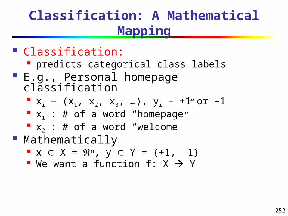
252

Classification: predicts categorical class labels

E.g., Personal homepage classification xi = (x1, x2, x3, …), yi = +1 or –1 x1 : # of a word “homepage” x2 : # of a word “welcome”

Mathematically x X = n, y Y = {+1, –1} We want a function f: X Y

Classification: A Mathematical Mapping

253

Linear Classification

Binary Classification problem

The data above the red line belongs to class ‘x’

The data below red line belongs to class ‘o’

Examples: SVM, Perceptron, Probabilistic Classifiersx

xx

x

xx

x

x

x

x ooo

oo

o

o

o

o o

oo

o

254

Discriminative Classifiers

Advantages prediction accuracy is generally high

As compared to Bayesian methods – in general robust, works when training examples contain errors fast evaluation of the learned target function

Bayesian networks are normally slow Criticism

long training time difficult to understand the learned function (weights)

Bayesian networks can be used easily for pattern discovery

not easy to incorporate domain knowledge Easy in the form of priors on the data or distributions

255

Perceptron & Winnow

• Vector: x, w

• Scalar: x, y, w

Input: {(x1, y1), …}

Output: classification function f(x)

f(xi) > 0 for yi = +1

f(xi) < 0 for yi = -1

f(x) => wx + b = 0

or w1x1+w2x2+b = 0

x1

x2

• Perceptron: update W additively

• Winnow: update W multiplicatively

256

Classification by Backpropagation

Backpropagation: A neural network learning algorithm Started by psychologists and neurobiologists to develop

and test computational analogues of neurons A neural network: A set of connected input/output units

where each connection has a weight associated with it During the learning phase, the network learns by

adjusting the weights so as to be able to predict the correct class label of the input tuples

Also referred to as connectionist learning due to the connections between units

257

Neural Network as a Classifier

Weakness Long training time Require a number of parameters typically best determined

empirically, e.g., the network topology or ``structure." Poor interpretability: Difficult to interpret the symbolic meaning

behind the learned weights and of ``hidden units" in the network Strength

High tolerance to noisy data Ability to classify untrained patterns Well-suited for continuous-valued inputs and outputs Successful on a wide array of real-world data Algorithms are inherently parallel Techniques have recently been developed for the extraction of

rules from trained neural networks

258

A Neuron (= a perceptron)

The n-dimensional input vector x is mapped into variable y by means of the scalar product and a nonlinear function mapping

k-

f

weighted sum

Inputvector x

output y

Activationfunction

weightvector w

w0

w1

wn

x0

x1

xn

)sign(y

ExampleFor n

0ikii xw

259

A Multi-Layer Feed-Forward Neural Network

Output layer

Input layer

Hidden layer

Output vector

Input vector: X

wij

i

jiijj OwI

jIje

O

1

1

))(1( jjjjj OTOOErr

jkk

kjjj wErrOOErr )1(

ijijij OErrlww )(jjj Errl)(

260

How A Multi-Layer Neural Network Works?

The inputs to the network correspond to the attributes measured for each training tuple

Inputs are fed simultaneously into the units making up the input layer

They are then weighted and fed simultaneously to a hidden layer The number of hidden layers is arbitrary, although usually only one The weighted outputs of the last hidden layer are input to units

making up the output layer, which emits the network's prediction The network is feed-forward in that none of the weights cycles back

to an input unit or to an output unit of a previous layer From a statistical point of view, networks perform nonlinear

regression: Given enough hidden units and enough training samples, they can closely approximate any function

261

Defining a Network Topology

First decide the network topology: # of units in the input layer, # of hidden layers (if > 1), # of units in each hidden layer, and # of units in the output layer

Normalizing the input values for each attribute measured in the training tuples to [0.0—1.0]

One input unit per domain value, each initialized to 0 Output, if for classification and more than two

classes, one output unit per class is used Once a network has been trained and its accuracy is

unacceptable, repeat the training process with a different network topology or a different set of initial weights

262

Backpropagation

Iteratively process a set of training tuples & compare the network's prediction with the actual known target value

For each training tuple, the weights are modified to minimize the mean squared error between the network's prediction and the actual target value

Modifications are made in the “backwards” direction: from the output layer, through each hidden layer down to the first hidden layer, hence “backpropagation”

Steps Initialize weights (to small random #s) and biases in the network Propagate the inputs forward (by applying activation function) Backpropagate the error (by updating weights and biases) Terminating condition (when error is very small, etc.)

263

Backpropagation and Interpretability

Efficiency of backpropagation: Each epoch (one interation through the training set) takes O(|D| * w), with |D| tuples and w weights, but # of epochs can be exponential to n, the number of inputs, in the worst case

Rule extraction from networks: network pruning Simplify the network structure by removing weighted links that

have the least effect on the trained network Then perform link, unit, or activation value clustering The set of input and activation values are studied to derive rules

describing the relationship between the input and hidden unit layers

Sensitivity analysis: assess the impact that a given input variable has on a network output. The knowledge gained from this analysis can be represented in rules

264

Associative Classification

Associative classification Association rules are generated and analyzed for use in classification

Search for strong associations between frequent patterns

(conjunctions of attribute-value pairs) and class labels

Classification: Based on evaluating a set of rules in the form of

P1 ^ p2 … ^ pl “Aclass = C” (conf, sup)

Why effective? It explores highly confident associations among multiple attributes

and may overcome some constraints introduced by decision-tree

induction, which considers only one attribute at a time

In many studies, associative classification has been found to be

more accurate than some traditional classification methods, such as

C4.5

265

Typical Associative Classification Methods

CBA (Classification By Association: Liu, Hsu & Ma, KDD’98) Mine association possible rules in the form of

Cond-set (a set of attribute-value pairs) class label Build classifier: Organize rules according to decreasing precedence

based on confidence and then support CMAR (Classification based on Multiple Association Rules: Li, Han, Pei, ICDM’01)

Classification: Statistical analysis on multiple rules CPAR (Classification based on Predictive Association Rules: Yin & Han, SDM’03)

Generation of predictive rules (FOIL-like analysis) High efficiency, accuracy similar to CMAR

RCBT (Mining top-k covering rule groups for gene expression data, Cong et al.

SIGMOD’05) Explore high-dimensional classification, using top-k rule groups Achieve high classification accuracy and high run-time efficiency

266

A Closer Look at CMAR

CMAR (Classification based on Multiple Association Rules: Li, Han, Pei, ICDM’01)

Efficiency: Uses an enhanced FP-tree that maintains the distribution of class labels among tuples satisfying each frequent itemset

Rule pruning whenever a rule is inserted into the tree Given two rules, R1 and R2, if the antecedent of R1 is more general

than that of R2 and conf(R1) ≥ conf(R2), then R2 is pruned Prunes rules for which the rule antecedent and class are not

positively correlated, based on a χ2 test of statistical significance Classification based on generated/pruned rules

If only one rule satisfies tuple X, assign the class label of the rule If a rule set S satisfies X, CMAR

divides S into groups according to class labels uses a weighted χ2 measure to find the strongest group

of rules, based on the statistical correlation of rules within a group

assigns X the class label of the strongest group

267

Associative Classification May Achieve High Accuracy and Efficiency (Cong et al.

SIGMOD05)

268

The k-Nearest Neighbor Algorithm

All instances correspond to points in the n-D space

The nearest neighbor are defined in terms of Euclidean distance, dist(X1, X2)

Target function could be discrete- or real- valued

For discrete-valued, k-NN returns the most common value among the k training examples nearest to xq

Vonoroi diagram: the decision surface induced by 1-NN for a typical set of training examples

.

_+

_ xq

+

_ _+

_

_

+

.

..

. .

269

Discussion on the k-NN Algorithm

k-NN for real-valued prediction for a given unknown tuple Returns the mean values of the k nearest neighbors

Distance-weighted nearest neighbor algorithm Weight the contribution of each of the k neighbors according

to their distance to the query xq

Give greater weight to closer neighbors Robust to noisy data by averaging k-nearest neighbors Curse of dimensionality: distance between neighbors

could be dominated by irrelevant attributes To overcome it, axes stretch or elimination of the least

relevant attributes

2),(1

ixqxdw

270

Case-Based Reasoning (CBR)

CBR: Uses a database of problem solutions to solve new problems Store symbolic description (tuples or cases)—not points in a

Euclidean space Applications: Customer-service (product-related diagnosis), legal

ruling Methodology

Instances represented by rich symbolic descriptions (e.g., function graphs)

Search for similar cases, multiple retrieved cases may be combined Tight coupling between case retrieval, knowledge-based reasoning,

and problem solving Challenges

Find a good similarity metric Indexing based on syntactic similarity measure, and when failure,

backtracking, and adapting to additional cases

271

Genetic Algorithms (GA)

Genetic Algorithm: based on an analogy to biological evolution An initial population is created consisting of randomly

generated rules Each rule is represented by a string of bits E.g., if A1 and ¬A2 then C2 can be encoded as 100

If an attribute has k > 2 values, k bits can be used Based on the notion of survival of the fittest, a new population

is formed to consist of the fittest rules and their offsprings The fitness of a rule is represented by its classification accuracy

on a set of training examples Offsprings are generated by crossover and mutation The process continues until a population P evolves when each

rule in P satisfies a prespecified threshold Slow but easily parallelizable

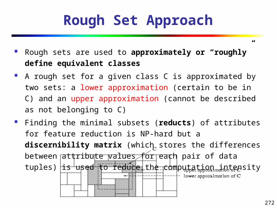
272

Rough Set Approach

Rough sets are used to approximately or “roughly” define equivalent classes

A rough set for a given class C is approximated by two sets: a lower approximation (certain to be in C) and an upper approximation (cannot be described as not belonging to C)

Finding the minimal subsets (reducts) of attributes for feature reduction is NP-hard but a discernibility matrix (which stores the differences between attribute values for each pair of data tuples) is used to reduce the computation intensity

273

Fuzzy Set Approaches

Fuzzy logic uses truth values between 0.0 and 1.0 to represent the degree of membership (such as using fuzzy membership graph)

Attribute values are converted to fuzzy values e.g., income is mapped into the discrete categories {low,

medium, high} with fuzzy values calculated For a given new sample, more than one fuzzy value

may apply Each applicable rule contributes a vote for

membership in the categories Typically, the truth values for each predicted

category are summed, and these sums are combined

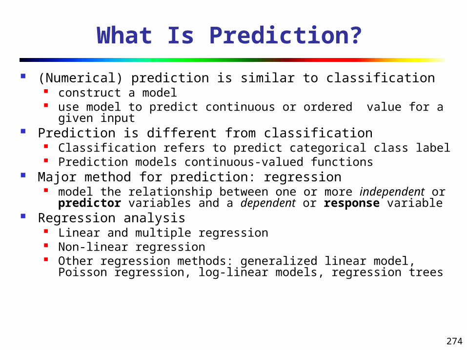
274

What Is Prediction?

(Numerical) prediction is similar to classification construct a model use model to predict continuous or ordered value for a given

input Prediction is different from classification

Classification refers to predict categorical class label Prediction models continuous-valued functions

Major method for prediction: regression model the relationship between one or more independent or

predictor variables and a dependent or response variable Regression analysis

Linear and multiple regression Non-linear regression Other regression methods: generalized linear model, Poisson

regression, log-linear models, regression trees

275

Linear Regression

Linear regression: involves a response variable y and a single predictor variable x

y = w0 + w1 x

where w0 (y-intercept) and w1 (slope) are regression coefficients

Method of least squares: estimates the best-fitting straight line

Multiple linear regression: involves more than one predictor variable Training data is of the form (X1, y1), (X2, y2),…, (X|D|, y|D|)

Ex. For 2-D data, we may have: y = w0 + w1 x1+ w2 x2

Solvable by extension of least square method or using SAS, S-Plus Many nonlinear functions can be transformed into the above

||

1

2

||

1

)(

))((

1 D

ii

D

iii

xx

yyxxw xwyw

10

276

Some nonlinear models can be modeled by a polynomial function

A polynomial regression model can be transformed into linear regression model. For example,

y = w0 + w1 x + w2 x2 + w3 x3

convertible to linear with new variables: x2 = x2, x3= x3

y = w0 + w1 x + w2 x2 + w3 x3 Other functions, such as power function, can also be

transformed to linear model Some models are intractable nonlinear (e.g., sum of

exponential terms) possible to obtain least square estimates through extensive

calculation on more complex formulae

Nonlinear Regression

277

Generalized linear model: Foundation on which linear regression can be applied to modeling

categorical response variables Variance of y is a function of the mean value of y, not a constant Logistic regression: models the prob. of some event occurring as a

linear function of a set of predictor variables Poisson regression: models the data that exhibit a Poisson

distribution Log-linear models: (for categorical data)

Approximate discrete multidimensional prob. distributions Also useful for data compression and smoothing

Regression trees and model trees Trees to predict continuous values rather than class labels

Other Regression-Based Models

278

Regression Trees and Model Trees

Regression tree: proposed in CART system (Breiman et al.

1984) CART: Classification And Regression Trees

Each leaf stores a continuous-valued prediction

It is the average value of the predicted attribute for the training

tuples that reach the leaf

Model tree: proposed by Quinlan (1992) Each leaf holds a regression model—a multivariate linear

equation for the predicted attribute

A more general case than regression tree

Regression and model trees tend to be more accurate than

linear regression when the data are not represented well by a

simple linear model

279

Predictive modeling: Predict data values or construct generalized linear models based on the database data

One can only predict value ranges or category distributions

Method outline: Minimal generalization Attribute relevance analysis Generalized linear model construction Prediction

Determine the major factors which influence the prediction Data relevance analysis: uncertainty measurement,

entropy analysis, expert judgement, etc. Multi-level prediction: drill-down and roll-up analysis

Predictive Modeling in Multidimensional Databases

280

Prediction: Numerical Data

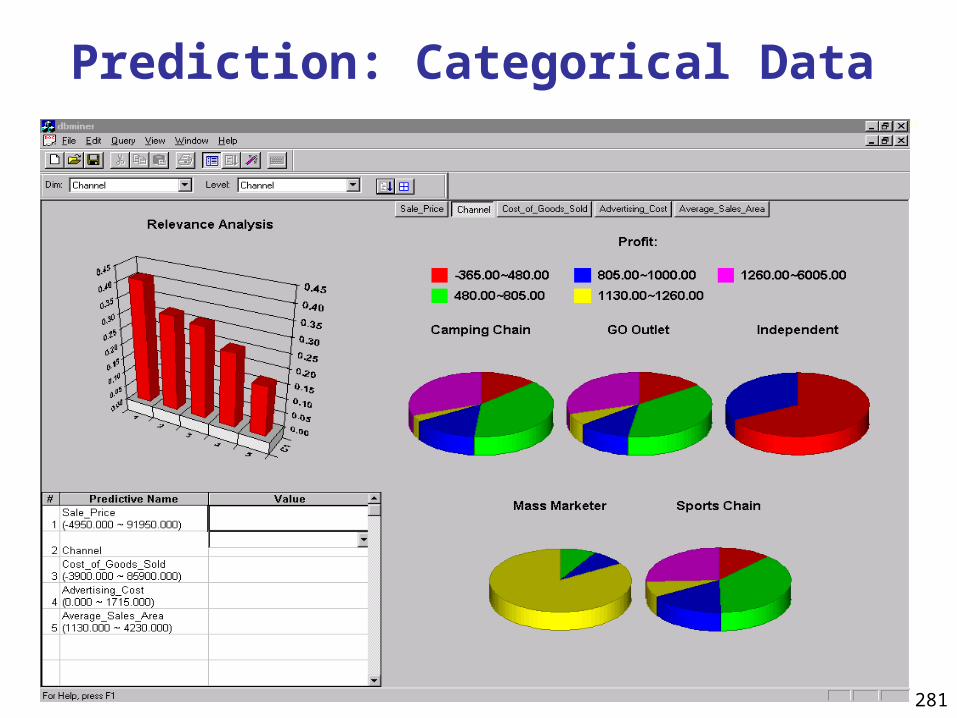
281

Prediction: Categorical Data

282

Classifier Accuracy Measures

Accuracy of a classifier M, acc(M): percentage of test set tuples that are correctly classified by the model M Error rate (misclassification rate) of M = 1 – acc(M) Given m classes, CMi,j, an entry in a confusion matrix, indicates #

of tuples in class i that are labeled by the classifier as class j Alternative accuracy measures (e.g., for cancer diagnosis)

sensitivity = t-pos/pos /* true positive recognition rate */specificity = t-neg/neg /* true negative recognition rate */precision = t-pos/(t-pos + f-pos)accuracy = sensitivity * pos/(pos + neg) + specificity * neg/(pos +

neg) This model can also be used for cost-benefit analysis

classes buy_computer = yes

buy_computer = no

total recognition(%)

buy_computer = yes

6954 46 7000 99.34

buy_computer = no

412 2588 3000 86.27

total 7366 2634 10000

95.52

C1 C2

C1True positive False

negative

C2False

positiveTrue negative

283

UNIT IV- Cluster Analysis

1. What is Cluster Analysis?

2. Types of Data in Cluster Analysis

3. A Categorization of Major Clustering Methods

4. Partitioning Methods

5. Outlier Analysis

284

What is Cluster Analysis?

Cluster: a collection of data objects Similar to one another within the same cluster Dissimilar to the objects in other clusters

Cluster analysis Finding similarities between data according to the

characteristics found in the data and grouping similar data objects into clusters

Unsupervised learning: no predefined classes Typical applications

As a stand-alone tool to get insight into data distribution As a preprocessing step for other algorithms

285

Clustering: Rich Applications and Multidisciplinary Efforts

Pattern Recognition Spatial Data Analysis

Create thematic maps in GIS by clustering feature spaces Detect spatial clusters or for other spatial mining tasks

Image Processing Economic Science (especially market research) WWW

Document classification Cluster Weblog data to discover groups of similar access

patterns

286

Examples of Clustering Applications

Marketing: Help marketers discover distinct groups in their

customer bases, and then use this knowledge to develop

targeted marketing programs

Land use: Identification of areas of similar land use in an

earth observation database

Insurance: Identifying groups of motor insurance policy

holders with a high average claim cost

City-planning: Identifying groups of houses according to their

house type, value, and geographical location

Earth-quake studies: Observed earth quake epicenters

should be clustered along continent faults

287

Quality: What Is Good Clustering?

A good clustering method will produce high quality

clusters with high intra-class similarity

low inter-class similarity

The quality of a clustering result depends on both

the similarity measure used by the method and its

implementation

The quality of a clustering method is also

measured by its ability to discover some or all of

the hidden patterns

288

Measure the Quality of Clustering

Dissimilarity/Similarity metric: Similarity is expressed in terms of a distance function, typically metric: d(i, j)

There is a separate “quality” function that measures the “goodness” of a cluster.

The definitions of distance functions are usually very different for interval-scaled, boolean, categorical, ordinal ratio, and vector variables.

Weights should be associated with different variables based on applications and data semantics.

It is hard to define “similar enough” or “good enough” the answer is typically highly subjective.

289

Requirements of Clustering in Data Mining

Scalability Ability to deal with different types of attributes Ability to handle dynamic data Discovery of clusters with arbitrary shape Minimal requirements for domain knowledge to

determine input parameters Able to deal with noise and outliers Insensitive to order of input records High dimensionality Incorporation of user-specified constraints Interpretability and usability

290

Data Structures

Data matrix (two modes)

Dissimilarity matrix (one mode)

npx...nfx...n1x

...............ipx...ifx...i1x

...............1px...1fx...11x

0...)2,()1,(

:::

)2,3()

...ndnd

0dd(3,1

0d(2,1)

0

291

Type of data in clustering analysis

Interval-scaled variables

Binary variables

Nominal, ordinal, and ratio variables

Variables of mixed types

292

Interval-valued variables

Standardize data Calculate the mean absolute deviation:

where

Calculate the standardized measurement (z-score)

Using mean absolute deviation is more robust than

using standard deviation

.)...21

1nffff

xx(xn m

|)|...|||(|121 fnffffff

mxmxmxns

f

fifif s

mx z

293

Similarity and Dissimilarity Between Objects

Distances are normally used to measure the similarity or dissimilarity between two data objects

Some popular ones include: Minkowski distance:

where i = (xi1, xi2, …, xip) and j = (xj1, xj2, …, xjp) are two p-

dimensional data objects, and q is a positive integer

If q = 1, d is Manhattan distance

qq

pp

qq

jx

ix

jx

ix

jx

ixjid )||...|||(|),(

2211

||...||||),(2211 pp jxixjxixjxixjid

294

Similarity and Dissimilarity Between Objects (Cont.)

If q = 2, d is Euclidean distance:

Properties

d(i,j) 0 d(i,i) = 0 d(i,j) = d(j,i) d(i,j) d(i,k) + d(k,j)

Also, one can use weighted distance, parametric Pearson product moment correlation, or other disimilarity measures

)||...|||(|),( 22

22

2

11 pp jx

ix

jx

ix

jx

ixjid

295

Binary Variables

A contingency table for binary

data

Distance measure for

symmetric binary variables:

Distance measure for

asymmetric binary variables:

Jaccard coefficient (similarity

measure for asymmetric

binary variables):

dcbacb jid

),(

cbacb jid

),(

pdbcasum

dcdc

baba

sum

0

1

01

Object i

Object j

cbaa jisim

Jaccard ),(

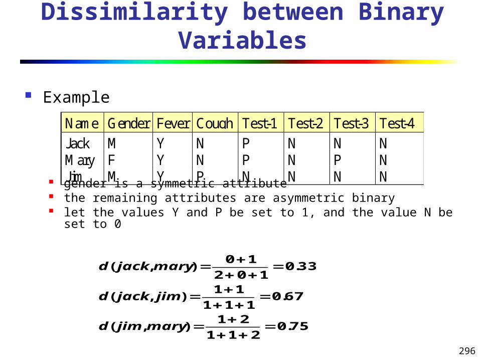
296

Dissimilarity between Binary Variables

Example

gender is a symmetric attribute the remaining attributes are asymmetric binary let the values Y and P be set to 1, and the value N be set to 0

Name Gender Fever Cough Test-1 Test-2 Test-3 Test-4

Jack M Y N P N N NMary F Y N P N P NJim M Y P N N N N

75.0211

21),(

67.0111

11),(

33.0102

10),(

maryjimd

jimjackd

maryjackd

297

Nominal Variables

A generalization of the binary variable in that it can take more than 2 states, e.g., red, yellow, blue, green

Method 1: Simple matching m: # of matches, p: total # of variables

Method 2: use a large number of binary variables creating a new binary variable for each of the M nominal

states

pmpjid ),(

298

Ordinal Variables

An ordinal variable can be discrete or continuous Order is important, e.g., rank Can be treated like interval-scaled

replace xif by their rank

map the range of each variable onto [0, 1] by replacing i-th object in the f-th variable by

compute the dissimilarity using methods for interval-scaled variables

11

f

ifif M

rz

},...,1{fif

Mr

299

Ratio-Scaled Variables

Ratio-scaled variable: a positive measurement on a nonlinear scale, approximately at exponential scale, such as AeBt or Ae-Bt

Methods: treat them like interval-scaled variables—not a good

choice! (why?—the scale can be distorted) apply logarithmic transformation

yif = log(xif) treat them as continuous ordinal data treat their rank as

interval-scaled

300

Variables of Mixed Types

A database may contain all the six types of variables symmetric binary, asymmetric binary, nominal, ordinal,

interval and ratio One may use a weighted formula to combine their

effects

f is binary or nominal:

dij(f) = 0 if xif = xjf , or dij

(f) = 1 otherwise f is interval-based: use the normalized distance f is ordinal or ratio-scaled

compute ranks rif and and treat zif as interval-scaled

)(1

)()(1),(

fij

pf

fij

fij

pf

djid

1

1

f

if

Mrz

if

301

Vector Objects

Vector objects: keywords in documents, gene features in micro-arrays, etc.

Broad applications: information retrieval, biologic taxonomy, etc.

Cosine measure

A variant: Tanimoto coefficient

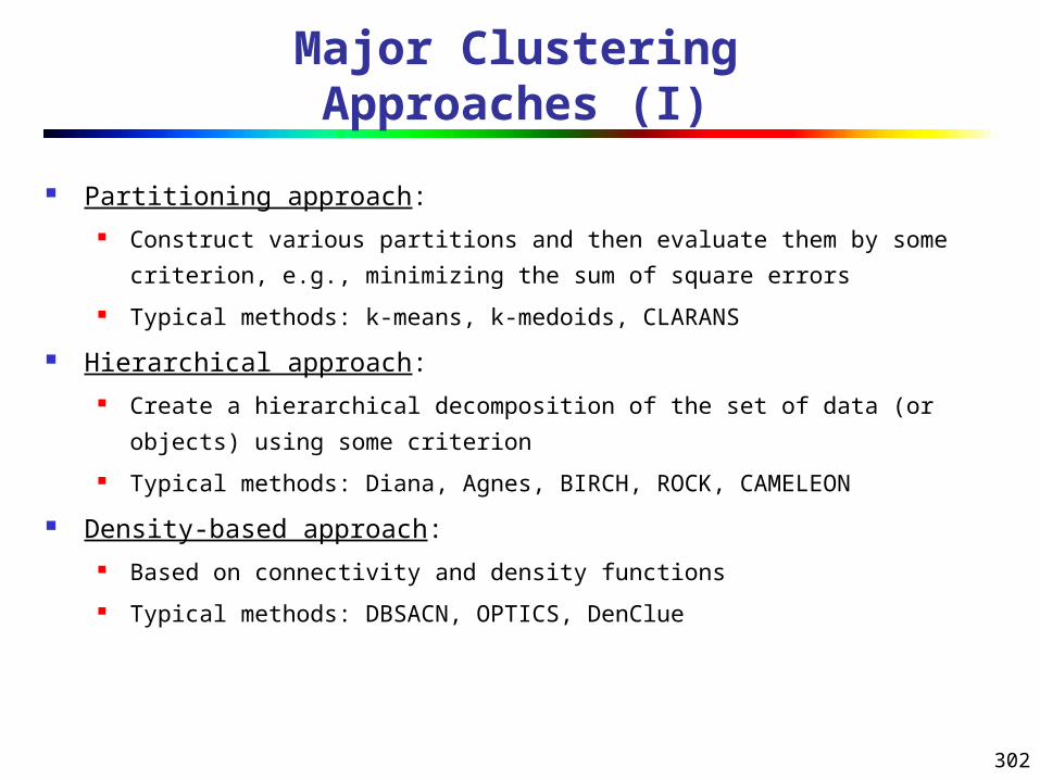
302

Major Clustering Approaches (I)

Partitioning approach: Construct various partitions and then evaluate them by some criterion,

e.g., minimizing the sum of square errors

Typical methods: k-means, k-medoids, CLARANS

Hierarchical approach: Create a hierarchical decomposition of the set of data (or objects) using

some criterion

Typical methods: Diana, Agnes, BIRCH, ROCK, CAMELEON

Density-based approach: Based on connectivity and density functions

Typical methods: DBSACN, OPTICS, DenClue

303

Major Clustering Approaches (II)

Grid-based approach: based on a multiple-level granularity structure

Typical methods: STING, WaveCluster, CLIQUE

Model-based: A model is hypothesized for each of the clusters and tries to find the best

fit of that model to each other

Typical methods: EM, SOM, COBWEB

Frequent pattern-based: Based on the analysis of frequent patterns

Typical methods: pCluster

User-guided or constraint-based: Clustering by considering user-specified or application-specific constraints

Typical methods: COD (obstacles), constrained clustering

304

Typical Alternatives to Calculate the Distance between Clusters

Single link: smallest distance between an element in one

cluster and an element in the other, i.e., dis(Ki, Kj) = min(tip, tjq)

Complete link: largest distance between an element in one

cluster and an element in the other, i.e., dis(Ki, Kj) = max(tip, tjq)

Average: avg distance between an element in one cluster and

an element in the other, i.e., dis(Ki, Kj) = avg(tip, tjq)

Centroid: distance between the centroids of two clusters, i.e.,

dis(Ki, Kj) = dis(Ci, Cj)

Medoid: distance between the medoids of two clusters, i.e.,

dis(Ki, Kj) = dis(Mi, Mj)

Medoid: one chosen, centrally located object in the cluster

305

Centroid, Radius and Diameter of a Cluster (for numerical data

sets) Centroid: the “middle” of a cluster

Radius: square root of average distance from any point of

the cluster to its centroid

Diameter: square root of average mean squared distance

between all pairs of points in the cluster

N

tNi ip

mC)(

1

N

mcip

tNi

mR

2)(1

)1(

2)(11

NNiq

tip

tNi

Ni

mD

306

Partitioning Algorithms: Basic Concept

Partitioning method: Construct a partition of a database D of n objects into a set of k clusters, s.t., min sum of squared distance

Given a k, find a partition of k clusters that optimizes the chosen partitioning criterion Global optimal: exhaustively enumerate all partitions Heuristic methods: k-means and k-medoids algorithms k-means (MacQueen’67): Each cluster is represented by the

center of the cluster k-medoids or PAM (Partition around medoids) (Kaufman &

Rousseeuw’87): Each cluster is represented by one of the objects in the cluster

21 )( mimKmt

km tC

mi

307

The K-Means Clustering Method

Given k, the k-means algorithm is implemented in four steps: Partition objects into k nonempty subsets Compute seed points as the centroids of the clusters

of the current partition (the centroid is the center, i.e., mean point, of the cluster)

Assign each object to the cluster with the nearest seed point

Go back to Step 2, stop when no more new assignment

308

The K-Means Clustering Method

Example

0

1

2

3

4

5

6

7

8

9

10

0 1 2 3 4 5 6 7 8 9 100

1

2

3

4

5

6

7

8

9

10

0 1 2 3 4 5 6 7 8 9 10

0

1

2

3

4

5

6

7

8

9

10

0 1 2 3 4 5 6 7 8 9 10

0

1

2

3

4

5

6

7

8

9

10

0 1 2 3 4 5 6 7 8 9 10

0

1

2

3

4

5

6

7

8

9

10

0 1 2 3 4 5 6 7 8 9 10

K=2

Arbitrarily choose K object as initial cluster center

Assign each objects to most similar center

Update the cluster means

Update the cluster means

reassignreassign

309

Comments on the K-Means Method

Strength: Relatively efficient: O(tkn), where n is # objects, k is # clusters, and t is # iterations. Normally, k, t << n.

Comparing: PAM: O(k(n-k)2 ), CLARA: O(ks2 + k(n-k)) Comment: Often terminates at a local optimum. The global

optimum may be found using techniques such as: deterministic annealing and genetic algorithms

Weakness Applicable only when mean is defined, then what about

categorical data? Need to specify k, the number of clusters, in advance Unable to handle noisy data and outliers Not suitable to discover clusters with non-convex shapes

310

Variations of the K-Means Method

A few variants of the k-means which differ in

Selection of the initial k means

Dissimilarity calculations

Strategies to calculate cluster means

Handling categorical data: k-modes (Huang’98)

Replacing means of clusters with modes

Using new dissimilarity measures to deal with categorical objects

Using a frequency-based method to update modes of clusters

A mixture of categorical and numerical data: k-prototype method

311

What Is the Problem of the K-Means Method?

The k-means algorithm is sensitive to outliers ! Since an object with an extremely large value may substantially

distort the distribution of the data.

K-Medoids: Instead of taking the mean value of the object in

a cluster as a reference point, medoids can be used, which is

the most centrally located object in a cluster.

0

1

2

3

4

5

6

7

8

9

10

0 1 2 3 4 5 6 7 8 9 100

1

2

3

4

5

6

7

8

9

10

0 1 2 3 4 5 6 7 8 9 10

312

The K-Medoids Clustering Method

Find representative objects, called medoids, in clusters

PAM (Partitioning Around Medoids, 1987)

starts from an initial set of medoids and iteratively replaces

one of the medoids by one of the non-medoids if it improves

the total distance of the resulting clustering

PAM works effectively for small data sets, but does not scale

well for large data sets

CLARA (Kaufmann & Rousseeuw, 1990)

CLARANS (Ng & Han, 1994): Randomized sampling

Focusing + spatial data structure (Ester et al., 1995)

313

A Typical K-Medoids Algorithm (PAM)

0

1

2

3

4

5

6

7

8

9

10

0 1 2 3 4 5 6 7 8 9 10

Total Cost = 20

0

1

2

3

4

5

6

7

8

9

10

0 1 2 3 4 5 6 7 8 9 10

K=2

Arbitrary choose k object as initial medoids

0

1

2

3

4

5

6

7

8

9

10

0 1 2 3 4 5 6 7 8 9 10

Assign each remaining object to nearest medoids Randomly select a

nonmedoid object,Oramdom

Compute total cost of swapping

0

1

2

3

4

5

6

7

8

9

10

0 1 2 3 4 5 6 7 8 9 10

Total Cost = 26

Swapping O and Oramdom

If quality is improved.

Do loop

Until no change

0

1

2

3

4

5

6

7

8

9

10

0 1 2 3 4 5 6 7 8 9 10

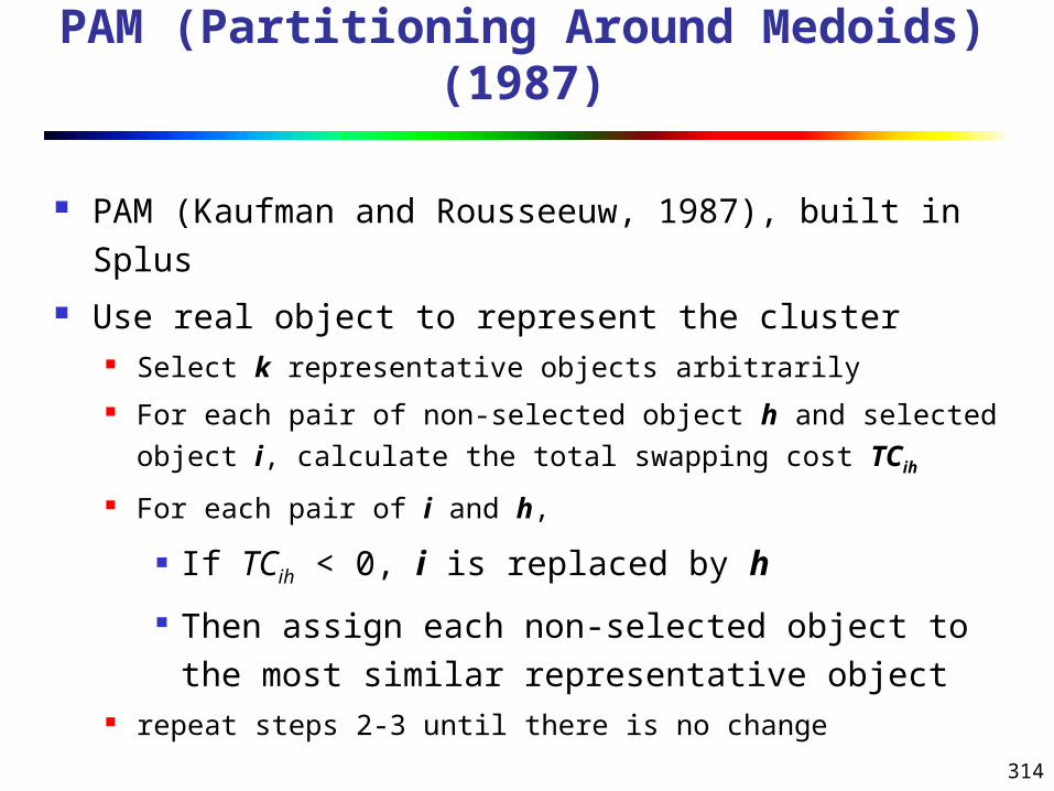
314

PAM (Partitioning Around Medoids) (1987)

PAM (Kaufman and Rousseeuw, 1987), built in Splus

Use real object to represent the cluster Select k representative objects arbitrarily For each pair of non-selected object h and selected object

i, calculate the total swapping cost TCih

For each pair of i and h,

If TCih < 0, i is replaced by h

Then assign each non-selected object to the most similar representative object

repeat steps 2-3 until there is no change

315

PAM Clustering: Total swapping cost TCih=jCjih

0

1

2

3

4

5

6

7

8

9

10

0 1 2 3 4 5 6 7 8 9 10

j

ih

t

Cjih = 0

0

1

2

3

4

5

6

7

8

9

10

0 1 2 3 4 5 6 7 8 9 10

t

i h

j

Cjih = d(j, h) - d(j, i)

0

1

2

3

4

5

6

7

8

9

10

0 1 2 3 4 5 6 7 8 9 10

h

i t

j

Cjih = d(j, t) - d(j, i)

0

1

2

3

4

5

6

7

8

9

10

0 1 2 3 4 5 6 7 8 9 10

t

ih j

Cjih = d(j, h) - d(j, t)

316

What Is the Problem with PAM?

Pam is more robust than k-means in the presence of noise and outliers because a medoid is less influenced by outliers or other extreme values than a mean

Pam works efficiently for small data sets but does not scale well for large data sets. O(k(n-k)2 ) for each iteration

where n is # of data,k is # of clusters Sampling based method,

CLARA(Clustering LARge Applications)

317

CLARA (Clustering Large Applications) (1990)

CLARA (Kaufmann and Rousseeuw in 1990)

Built in statistical analysis packages, such as S+

It draws multiple samples of the data set, applies PAM on each sample, and gives the best clustering as the output

Strength: deals with larger data sets than PAM Weakness:

Efficiency depends on the sample size A good clustering based on samples will not necessarily

represent a good clustering of the whole data set if the sample is biased

318

CLARANS (“Randomized” CLARA) (1994)

CLARANS (A Clustering Algorithm based on Randomized Search) (Ng and Han’94)

CLARANS draws sample of neighbors dynamically The clustering process can be presented as searching a

graph where every node is a potential solution, that is, a set of k medoids

If the local optimum is found, CLARANS starts with new randomly selected node in search for a new local optimum

It is more efficient and scalable than both PAM and CLARA Focusing techniques and spatial access structures may

further improve its performance (Ester et al.’95)

319

What Is Outlier Discovery?

What are outliers? The set of objects are considerably dissimilar from the

remainder of the data Example: Sports: Michael Jordon, Wayne Gretzky, ...

Problem: Define and find outliers in large data sets Applications:

Credit card fraud detection Telecom fraud detection Customer segmentation Medical analysis

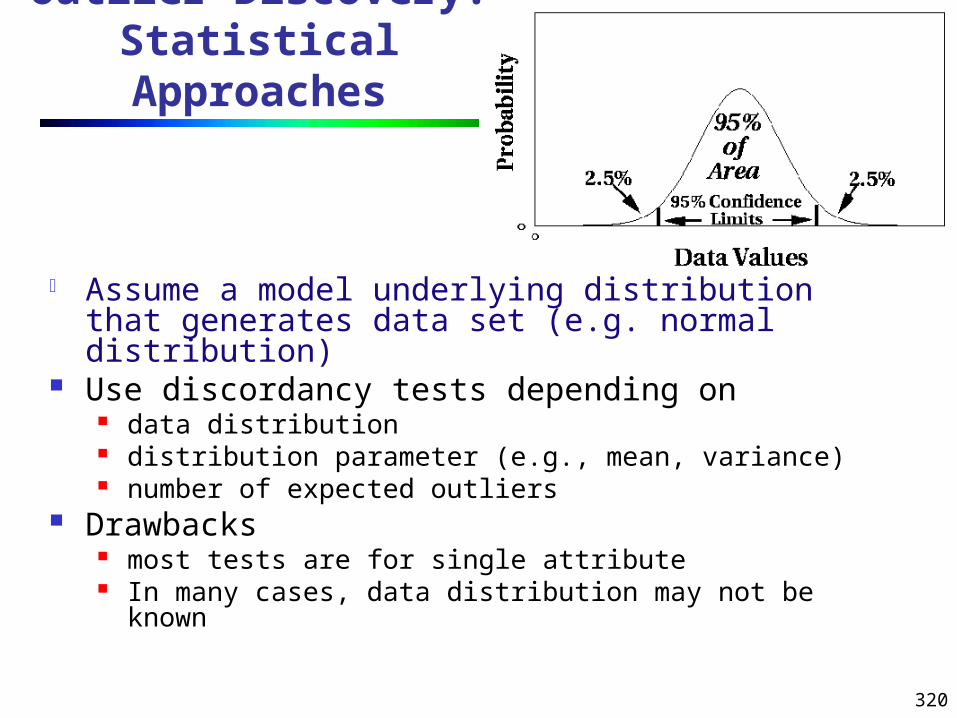
320

Outlier Discovery: Statistical

Approaches

Assume a model underlying distribution that generates data set (e.g. normal distribution)

Use discordancy tests depending on data distribution distribution parameter (e.g., mean, variance) number of expected outliers

Drawbacks most tests are for single attribute In many cases, data distribution may not be known

321

Outlier Discovery: Distance-Based Approach

Introduced to counter the main limitations imposed by statistical methods We need multi-dimensional analysis without knowing data

distribution Distance-based outlier: A DB(p, D)-outlier is an

object O in a dataset T such that at least a fraction p of the objects in T lies at a distance greater than D from O

Algorithms for mining distance-based outliers Index-based algorithm Nested-loop algorithm Cell-based algorithm

322

Density-Based Local Outlier

Detection

Distance-based outlier detection is based on global distance distribution

It encounters difficulties to identify outliers if data is not uniformly distributed

Ex. C1 contains 400 loosely distributed points, C2 has 100 tightly condensed points, 2 outlier points o1, o2

Distance-based method cannot identify o2 as an outlier

Need the concept of local outlier

Local outlier factor (LOF) Assume outlier is not

crisp Each point has a LOF

323

Outlier Discovery: Deviation-Based Approach

Identifies outliers by examining the main characteristics of objects in a group

Objects that “deviate” from this description are considered outliers

Sequential exception technique simulates the way in which humans can distinguish

unusual objects from among a series of supposedly like objects

OLAP data cube technique uses data cubes to identify regions of anomalies in large

multidimensional data

1 Chapter 1. Introduction Motivation: Why data mining? What is data mining? Data Mining: On what kind of data? Data mining functionality Major issues in.

Documents

data miningwhy data

data reduction

data archeology

data dredging

data warehousing

kind of data

relational data model

traditional data analysis