1 A Robust Bayesian Fusion Algorithm for Lane and ...web.eecs.umich.edu/~hero/Preprints/ma_vt03.pdf1 A Robust Bayesian Fusion Algorithm for Lane and Pavement boundary detection Bing

1

A Robust Bayesian Fusion Algorithm for Lane and

Pavement boundary detection

Bing Ma, Sridhar Lakshmanan, Alfred O. Hero

Abstract

In this paper we propose to jointly detect lane and pavement boundaries by fusing information from both optical and radar images acquired with the sensor

system mounted on the top of the host vehicle. The boundaries are described with concentric circular models. The optical and radar imaging processes are

modeled as Gaussian and log-normal probability densities. The multisensor fusion boundary detection problem is posed in a Bayesian framework and a maximum

a posteriori(MAP) estimate is employed to locate the lane and pavement boundaries. Since the circular model parameters possess compatible units and are in the

same order of magnitude, the estimation problem is much better conditioned than using the previous parabolic models, whose parameters are incompatible with

each other. This fusion algorithm achieves analytical integration of two different sensing modalities due to the validation of the likelihoods thatdescribe both optical

and radar imaging processes. Experimental results have shown that the fusion algorithm outperforms single sensor based boundary detection algorithms in a variety

of road scenarios.

I. I NTRODUCTION

Intelligent transportation systems (ITS) have attracted a great number of researchers’ interests in the past years. Among a variety

of ITS missions automated detection of lane and pavement boundaries is primary and essential for the control and maneuver of the

vehicle. It will provide necessary information for road departure warning, lane excursion warning, intelligent cruise control, and

ultimately, autonomous driving.

Lane and pavement boundary detection problems have been broadly studied in the field of intelligent transportation. Due to

the complicated nature of the road scenario, e.g., entry/exit ramps, occlusion from other vehicles, shadows, and varying outdoor

illumination, gradient based algorithms have shown their limitations in this boundary detection application [1]. Many state-of-

the-art systems for detecting and tracking lane and pavement boundaries usea priori shape models to mathematically describe

the appearance of these boundaries [1–6]. The use of prior shape models allows these systems to reject false boundaries (such as

entry/exit ramps) and also overcome image clutter (shadows) and occlusion.

Bing Ma was with the Department of Electrical Engineering and Computer Science at the University of Michigan, Ann Arbor. She is now with M-Vision, Inc.,

Belleville, MI 48111. E-mail: [email protected] .

Sridhar Lakshmanan is with the Department of Electrical and Computer Engineering, the University of Michigan, Dearborn, MI 48128. E-mail: laksh-

[email protected] .

Alfred O. Hero is with the Department of Electrical Engineering and Computer Science, the University of Michigan, Ann Arbor, MI 48109. E-mail:

[email protected] .

2

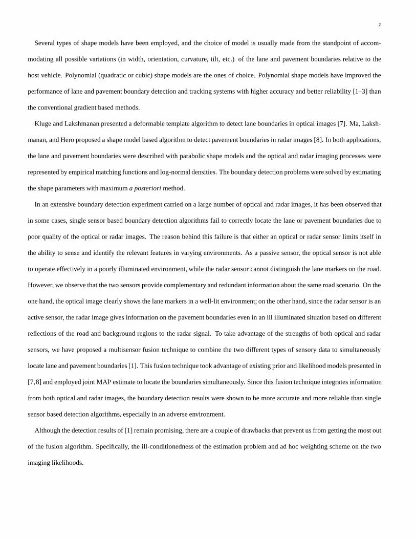
Several types of shape models have been employed, and the choice of model is usually made from the standpoint of accom-

modating all possible variations (in width, orientation, curvature, tilt, etc.) of the lane and pavement boundaries relative to the

host vehicle. Polynomial (quadratic or cubic) shape models are the ones of choice. Polynomial shape models have improved the

performance of lane and pavement boundary detection and tracking systems with higher accuracy and better reliability [1–3] than

the conventional gradient based methods.

Kluge and Lakshmanan presented a deformable template algorithm to detect lane boundaries in optical images [7]. Ma, Laksh-

manan, and Hero proposed a shape model based algorithm to detect pavement boundaries in radar images [8]. In both applications,

the lane and pavement boundaries were described with parabolic shape models and the optical and radar imaging processes were

represented by empirical matching functions and log-normal densities. The boundary detection problems were solved by estimating

the shape parameters with maximuma posteriorimethod.

In an extensive boundary detection experiment carried on a large number of optical and radar images, it has been observed that

in some cases, single sensor based boundary detection algorithms fail to correctly locate the lane or pavement boundaries due to

poor quality of the optical or radar images. The reason behind this failure is that either an optical or radar sensor limits itself in

the ability to sense and identify the relevant features in varying environments. As a passive sensor, the optical sensor is not able

to operate effectively in a poorly illuminated environment, while the radar sensor cannot distinguish the lane markers on the road.

However, we observe that the two sensors provide complementary and redundant information about the same road scenario. On the

one hand, the optical image clearly shows the lane markers in a well-lit environment; on the other hand, since the radar sensor is an

active sensor, the radar image gives information on the pavement boundaries even in an ill illuminated situation based on different

reflections of the road and background regions to the radar signal. To take advantage of the strengths of both optical and radar

sensors, we have proposed a multisensor fusion technique to combine the two different types of sensory data to simultaneously

locate lane and pavement boundaries [1]. This fusion technique took advantage of existing prior and likelihood models presented in

[7,8] and employed joint MAP estimate to locate the boundaries simultaneously. Since this fusion technique integrates information

from both optical and radar images, the boundary detection results were shown to be more accurate and more reliable than single

sensor based detection algorithms, especially in an adverse environment.

Although the detection results of [1] remain promising, there are a couple of drawbacks that prevent us from getting the most out

of the fusion algorithm. Specifically, the ill-conditionedness of the estimation problem and ad hoc weighting scheme on the two

imaging likelihoods.

3

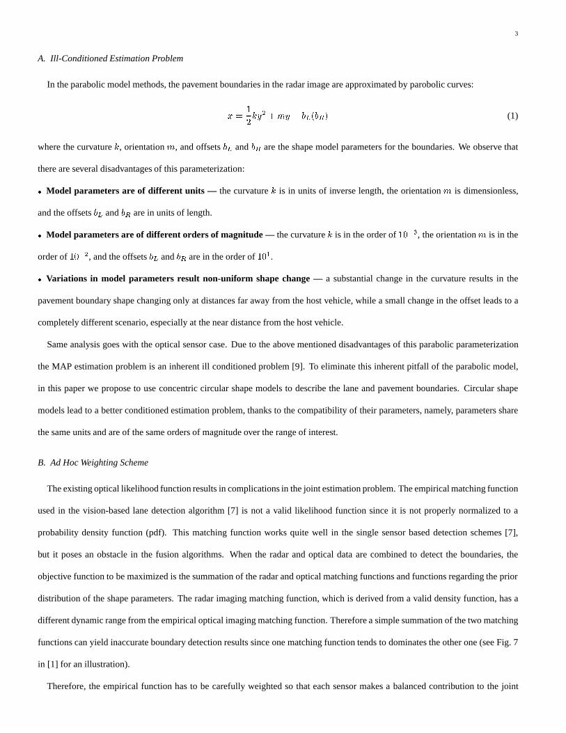
A. Ill-Conditioned Estimation Problem

In the parabolic model methods, the pavement boundaries in the radar image are approximated by parobolic curves:

x =1

2ky2 +my + bL(bR) (1)

where the curvaturek, orientationm, and offsetsbL andbR are the shape model parameters for the boundaries. We observe that

there are several disadvantages of this parameterization:

� Model parameters are of different units — the curvaturek is in units of inverse length, the orientationm is dimensionless,

and the offsetsbL andbR are in units of length.

� Model parameters are of different orders of magnitude —the curvaturek is in the order of10�3, the orientationm is in the

order of10�2, and the offsetsbL andbR are in the order of101.

� Variations in model parameters result non-uniform shape change —a substantial change in the curvature results in the

pavement boundary shape changing only at distances far away from the host vehicle, while a small change in the offset leads to a

completely different scenario, especially at the near distance from the host vehicle.

Same analysis goes with the optical sensor case. Due to the above mentioned disadvantages of this parabolic parameterization

the MAP estimation problem is an inherent ill conditioned problem [9]. To eliminate this inherent pitfall of the parabolic model,

in this paper we propose to use concentric circular shape models to describe the lane and pavement boundaries. Circular shape

models lead to a better conditioned estimation problem, thanks to the compatibility of their parameters, namely, parameters share

the same units and are of the same orders of magnitude over the range of interest.

B. Ad Hoc Weighting Scheme

The existing optical likelihood function results in complications in the joint estimation problem. The empirical matching function

used in the vision-based lane detection algorithm [7] is not a valid likelihood function since it is not properly normalized to a

probability density function (pdf). This matching function works quite well in the single sensor based detection schemes [7],

but it poses an obstacle in the fusion algorithms. When the radar and optical data are combined to detect the boundaries, the

objective function to be maximized is the summation of the radar and optical matching functions and functions regarding the prior

distribution of the shape parameters. The radar imaging matching function, which is derived from a valid density function, has a

different dynamic range from the empirical optical imaging matching function. Therefore a simple summation of the two matching

functions can yield inaccurate boundary detection results since one matching function tends to dominates the other one (see Fig. 7

in [1] for an illustration).

Therefore, the empirical function has to be carefully weighted so that each sensor makes a balanced contribution to the joint

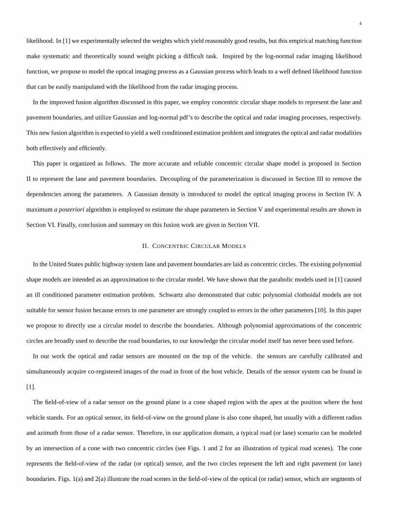
4

likelihood. In [1] we experimentally selected the weights which yield reasonably good results, but this empirical matching function

make systematic and theoretically sound weight picking a difficult task. Inspired by the log-normal radar imaging likelihood

function, we propose to model the optical imaging process as a Gaussian process which leads to a well defined likelihood function

that can be easily manipulated with the likelihood from the radar imaging process.

In the improved fusion algorithm discussed in this paper, we employ concentric circular shape models to represent the lane and

pavement boundaries, and utilize Gaussian and log-normal pdf’s to describe the optical and radar imaging processes, respectively.

This new fusion algorithm is expected to yield a well conditioned estimation problem and integrates the optical and radar modalities

both effectively and efficiently.

This paper is organized as follows. The more accurate and reliable concentric circular shape model is proposed in Section

II to represent the lane and pavement boundaries. Decoupling of the parameterization is discussed in Section III to remove the

dependencies among the parameters. A Gaussian density is introduced to model the optical imaging process in Section IV. A

maximuma posteriorialgorithm is employed to estimate the shape parameters in Section V and experimental results are shown in

Section VI. Finally, conclusion and summary on this fusion work are given in Section VII.

II. CONCENTRIC CIRCULAR MODELS

In the United States public highway system lane and pavement boundaries are laid as concentric circles. The existing polynomial

shape models are intended as an approximation to the circular model. We have shown that the parabolic models used in [1] caused

an ill conditioned parameter estimation problem. Schwartz also demonstrated that cubic polynomial clothoidal models are not

suitable for sensor fusion because errors in one parameter are strongly coupled to errors in the other parameters [10]. In this paper

we propose to directly use a circular model to describe the boundaries. Although polynomial approximations of the concentric

circles are broadly used to describe the road boundaries, to our knowledge the circular model itself has never been used before.

In our work the optical and radar sensors are mounted on the top of the vehicle. the sensors are carefully calibrated and

simultaneously acquire co-registered images of the road in front of the host vehicle. Details of the sensor system can be found in

[1].

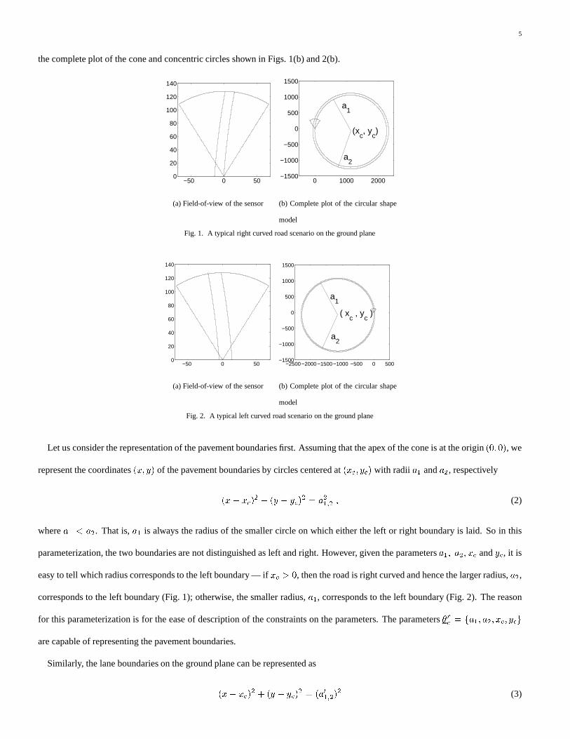
The field-of-view of a radar sensor on the ground plane is a cone shaped region with the apex at the position where the host

vehicle stands. For an optical sensor, its field-of-view on the ground plane is also cone shaped, but usually with a different radius

and azimuth from those of a radar sensor. Therefore, in our application domain, a typical road (or lane) scenario can be modeled

by an intersection of a cone with two concentric circles (see Figs. 1 and 2 for an illustration of typical road scenes). The cone

represents the field-of-view of the radar (or optical) sensor, and the two circles represent the left and right pavement (or lane)

boundaries. Figs. 1(a) and 2(a) illustrate the road scenes in the field-of-view of the optical (or radar) sensor, which are segments of

5

the complete plot of the cone and concentric circles shown in Figs. 1(b) and 2(b).

−50 0 500

20

40

60

80

100

120

140

(a) Field-of-view of the sensor

0 1000 2000−1500

−1000

−500

0

500

1000

1500

a1

a2

(xc, y

c)

(b) Complete plot of the circular shape

model

Fig. 1. A typical right curved road scenario on the ground plane

−50 0 500

20

40

60

80

100

120

140

(a) Field-of-view of the sensor

−2500−2000−1500−1000 −500 0 500−1500

−1000

−500

0

500

1000

1500

a1

a2

( xc , y

c )

(b) Complete plot of the circular shape

model

Fig. 2. A typical left curved road scenario on the ground plane

Let us consider the representation of the pavement boundaries first. Assuming that the apex of the cone is at the origin(0; 0), we

represent the coordinates(x; y) of the pavement boundaries by circles centered at(xc; yc) with radii a1 anda2, respectively

(x� xc)2 + (y � yc)

2 = a21;2 ; (2)

wherea1 < a2. That is,a1 is always the radius of the smaller circle on which either the left or right boundary is laid. So in this

parameterization, the two boundaries are not distinguished as left and right. However, given the parametersa1; a2; xc andyc, it is

easy to tell which radius corresponds to the left boundary — ifxc > 0, then the road is right curved and hence the larger radius,a2,

corresponds to the left boundary (Fig. 1); otherwise, the smaller radius,a1, corresponds to the left boundary (Fig. 2). The reason

for this parameterization is for the ease of description of the constraints on the parameters. The parameters�rc = fa1; a2; xc; ycg

are capable of representing the pavement boundaries.

Similarly, the lane boundaries on the ground plane can be represented as

(x� xc)2 + (y � yc)

2 = (a01;2)2 (3)

6

wherea01 anda02 are the radii of the circles that correspond to the lane boundaries. Then�oc = fa01; a02; xc; ycg are the shape

parameters for lane boundaries on the ground plane. Note that the lane and pavement boundaries share the same parameters

(xc; yc) since they are laid on concentric circles.

There are a number of advantages of the new parameterization over the polynomial shape models. First of all, the new model

better reflects the road shape of the real world. Circular shape models exactly describe the road boundaries, while parabolic shape

models only approximate the road boundaries. For the circular shape model, the six parametersa1; a2; a01; a

02; xc andyc have the

same units – that of length. In addition, their ranges of feasible values have the same orders of magnitude. On the contrary, the

parabolic shape parameters have different units and different dynamic ranges. We also observe that for both shape models, the

number of parameters are the same, or in other words neither model is more complex to describe than the other.

The domain of the radar image is actually the ground plane and (2) can be directly applied to model the shape of pavement

boundaries in the radar image.

The domain of the optical image, however, is a perspective projection of the road scenario on the ground plane, and therefore we

need to transform the optical image data and the lane boundary model onto the same image plane.

There are two possible approaches to accomplish this goal. One is similar to the technique used in the parabolic shape models

[11] — apply the perspective projection operator to the circular shape model (3) on the ground plane to obtain a lane boundary

shape model on the image plane. An alternative method is to project the optical image data onto the ground plane with the inverse

perspective projection while still using (3) to describe the lane boundaries. Note that in the second approach, the parameters of

the lane boundaries,fa01; a02; xc; ycg, have the same physical units (namely, units of length) and properties as the parameters of the

pavement boundaries,fa1; a2; xc; ycg. This is a desirable characteristic to ensure unit compatibility, and hence well-conditioned

estimation in the fusion algorithm. Therefore, we will take the second approach.

The projection of the optical image onto the ground plane is implemented by projecting the pixel positions to ground coordinates.

For each pixel with row and column(r; c) in the optical image plane, its corresponding Cartesian coordinates(x; y) on the ground

plane can be calculated by

y =h [1� r2f (r � cr)(cr � hz)]

rf (r � hz)

x = cf (c� cc)

sy2 + h2

1 + r2f (r � cr)2(4)

wherehz is the horizon row,h is the height of the focal point above the ground plane,rf is the height of a pixel on the image

plane divided by the focal length,cf is the width of a pixel on the image plane divided by the focal length, andcc andcr are one

half of the numbers of columns and rows, respectively. For the purpose of conciseness, during further algorithm derivation for lane

7

boundary detection, the optical image is referred to the projected optical image on the ground plane.

What sets the models apart are the constraints on the parameters in circular and parabolic shape models. These constraints are

imposed in order to result in a “feasible” pair of left and right lane and pavement boundaries. In the parabolic case, the feasibility

region is a hypercube with respect to the model parameters. In the circular model, the feasibility region is not so simple. The

feasibility region has the following restrictions:

1. The two circles corresponding to the pavement boundaries must intersect the cone. That is, the cone cannot be completely inside

the inner circle, neither can it be outside the outer circle (see Fig. 31). Such constraint on the model parameters can be represented

by

a1 � p1 � x2c + y2c � a2 + p2 (5)

wherep1 andp2 are two appropriately selected positive numbers that will allow the corresponding pavement boundaries to both

be offset to either the left or the right of the origin for extreme cases. Of course, the left boundary can be offset to the left of the

origin, and the right boundary to its right.

−500 0 500 1000

−800

−600

−400

−200

0

200

400

600

(a)

0 500 1000

−800

−600

−400

−200

0

200

400

600

(b)

Fig. 3. Cases where circles do not intersect the cone

2. The image data are acquired under the assumption that the host vehicle is still within the road (or at least within the shoulder).

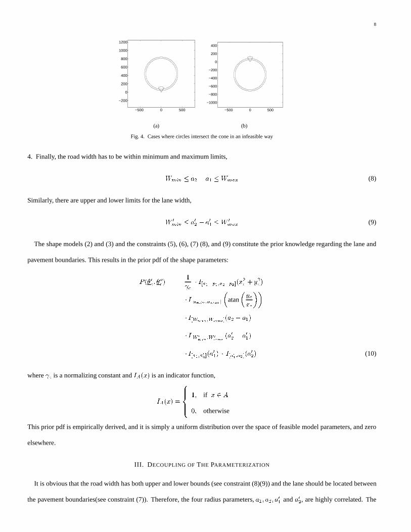
As such, the cases shown in Fig. 4 are not realistic as they correspond to scenarios when the host vehicle is entirely off the road.

The corresponding constraint on the model parameters is

�min � atan

�yc

xc

�� �max (6)

3. The lane should be positioned inside the road region, i.e., the two circles on which the lane boundaries are laid are between the

two circles on which the pavement boundaries are laid.

a1 < a01 < a02 < a2; (7)

1The plots in Figs. 3 and 4 only demonstrate the relationship between the circles and the cone. In order to make the plots easily readable, we enlarged thesize of

the cone and the width of the road, while reduced the size of the circles.

8

−500 0 500

−200

0

200

400

600

800

1000

1200

(a)

−500 0 500

−1000

−800

−600

−400

−200

0

200

400

(b)

Fig. 4. Cases where circles intersect the cone in an infeasible way

4. Finally, the road width has to be within minimum and maximum limits,

Wmin � a2 � a1 �Wmax (8)

Similarly, there are upper and lower limits for the lane width,

W 0min � a02 � a01 �W 0

max (9)

The shape models (2) and (3) and the constraints (5), (6), (7) (8), and (9) constitute the prior knowledge regarding the lane and

pavement boundaries. This results in the prior pdf of the shape parameters:

P (�rc ; �oc) =

1

c� I[a1�p1;a2+p2](x2c + y2c )

� I[�min;�max]

�atan

�yc

xc

��

� I[Wmin;Wmax](a2 � a1)

� I[W 0

min;W 0

max](a

02 � a01)

� I[a1;a0

2](a

01) � I[a0

1;a2](a

02) (10)

where c is a normalizing constant andIA(x) is an indicator function,

IA(x) =

8>><>>:

1; if x 2 A

0; otherwise

This prior pdf is empirically derived, and it is simply a uniform distribution over the space of feasible model parameters, and zero

elsewhere.

III. D ECOUPLING OFTHE PARAMETERIZATION

It is obvious that the road width has both upper and lower bounds (see constraint (8)(9)) and the lane should be located between

the pavement boundaries(see constraint (7)). Therefore, the four radius parameters,a1; a2; a01 anda02, are highly correlated. The

9

apex of the cone, where the host vehicle is located, is inside the road, at least on the shoulder. Therefore,xc andyc are constrained by

parametersa1 anda2 (see constraint (5)). The dependence among the parameters makes the parameter constraints very complicated,

as we have seen in (10). And more critically, the dependence among the parameters makes the estimation problem more difficult.

Namely, an estimation error of one parameter will result in errors in estimating other parameters.

As a remedy to the pitfalls caused by the parameterization, we propose an alternative parameter set to describe the boundaries in

order to remove the high correlation among the shape parameters.

Let us remove the dependence among the pavement boundary parameters first. Instead of using highly correlated parametersa1

anda2, we propose to use parametersa1 andw2, the smaller radius and the distance between the left and right pavement boundaries.

And to eliminate the dependence betweena1 andxc, we replacexc with x0c, the horizontal coordinate of the intersection point of the

circle with radiusa1 and the line segment passing the circle center and parallel to thex axis. Fig. 5(a) illustrates the new parameter

set with right curved pavement boundaries. In this case, the center is to the right of the circles. The right pavement boundary

corresponds to the circle with radiusa1. C is the center of the circles.CA is a line segment parallel to thex axis and passing

through the pointC. A is the intersection of the line segmentCA and the circle with radiusa1. Then the Cartesian coordinates of

A are(x0c; yc), and

xc = x0c + a1: (11)

y

xO

A : (x0c; yc) C : (xc; yc)w2

(a) the center is to the right of the road

O x

y

A : (x0c; yc)

C : (xc; yc) w2

(b) the center is to the left of the road

Fig. 5. Decoupled parameterization of the boundary shape models

The radius of the left boundary,a2, can be represented by the summation of the radius of the right boundary,a1, and the distance

between the two boundaries,w2.

a2 = a1 + w2 (12)

Fig. 5(b) shows left curved boundaries. In this case, the center is to the left of the circles and the left pavement boundary

10

corresponds to the circle with radiusa1. LetCA still be the line segment parallel to thex axis connecting two points,C andA.

Then (12) holds for this case, too. AndA’s coordinates(x0c; yc) satisfy

xc = x0c � a1 (13)

In order to unify (11) and (13) we define a new parametera as

a =

8>><>>:

a1; if the center is to the right of the road,

�a1; otherwise:

(14)

In other words, the magnitude ofa is the radius value of the smaller circle, and the sign ofa depends on the relative position of the

center and the boundaries. Then it is immediate to geta1 givena,

a1 = jaj (15)

With this new parametera, rewriting (11) and (13) in a united form, we have

xc = x0c + a: (16)

And with (15), (12) can be rewritten as

a2 = w2 + jaj (17)

Given the new pavement shape parametersfa; w2; x0c; ycg, the previous parametersfa1; a2; xc; ycg can be easily calculated with

the relationships (15), (16), and (17). That is,fa; w2; x0c; ycg are capable of representing the pavement boundaries and they have

the advantage of being independent of one another.

To eliminate the dependence among the lane shape parametersfa01; a02; xc; ycg, a similar decoupling technique is applied. The

new lane shape parametersfa0; w02; x

0c; ycg satisfy

a0 =

8>><>>:

a01; if the center is to the right of the road,

�a01; otherwise:

(18)

w02 = a02 � ja0j (19)

x0c = xc � a0 (20)

In the fusion framework, we could easily define the joint shape parameters asfa; w2; a0; w0

2; x0c; ycg. In this parameterization, the

lane and pavement boundariesa anda0 are still coupled, which is not a desirable property. To remove this remaining dependence,

we propose a unified parameter set for both lane and pavement boundaries.

11

In Fig. 6, we illustrate the unified shape parametersfa; w2; w01; w

02; x

0c; ycg for both lane and pavement boundaries. In this plot,

the solid curves represent the pavement boundaries and the dashed curves represent the lane boundaries. For this parameter set,a

is defined by (14). The distance parametersw2; w01; andw0

2 satisfy

a2 = w2 + jaj (21)

a01 = w01 + jaj (22)

a02 = w02 + jaj (23)

And thex coordinate of the circle center is determined by (16).

y

xO

a

A : (x0c; yc) C : (xc; yc)w2

w01

w02

Fig. 6. Unified parameterization for both lane and pavement boundaries

The parameters�c = fa; w2; w01; w

02; x

0c; ycg are able to represent the lane and pavement boundaries and they are independent

from each other. In our fusion algorithm, we will use this parameterization to describe the prior information on the boundaries.

The constraints on�c can be easily derived from the previous stated constraints onfa1; a2; a01; a02; xc; ycg as follows

P (�c) =1

c� I[jaj�p1;jaj+w2+p2]((a+ x0c)

2 + y2c )

� I[�min;�max]

�atan

�yc

a+ x0c

��

� I[Wmin;Wmax](w2) � I[W 0

min;W 0

max](w

02 � w0

1)

� I[0;w0

2](w

01) � I[w0

1;w2](w

02); (24)

where c is a normalizing constant.

It is straightforward to derive the shape model parameters in the radar and optical images from�c: �rc = fjaj; jaj+w2; x

0c+a; ycg,

and�oc = fjaj+ w01; jaj+ w0

2; x0c + a; ycg.

12

IV. I MAGING LIKELIHOODS

We have seen that in the fusion algorithm presented in [1], the joint MAP estimation is approximated by an ad hoc empirical

parameter estimation. The root cause for this approximation is that the optical and radar matching functions are incompatible

and different weights have to be imposed on them when they are combined in the fusion framework. Although the radar imaging

process is modeled with a log-normal density, the optical imaging process is described with an empirical likelihood function, which

makes it impossible to theoretically derive the weights.

The key to avoid ad hoc approximation of the joint MAP estimation is to use real probability densities to represent both radar

and optical imaging processes. With proper likelihood functions, no weighting scheme is needed in the proposed fusion algorithm.

A. Radar Imaging Likelihood

We will continue to use the log-normal pdf employed in [1] to model the radar imaging process. To keep this paper self-contained

we give the pdf in [1] here. The true boundaries of the pavement separate the observed radar image into three regions associated

with the road surface, the left side of the road, and the right side of the road. LetL = f(r; �), 1 � r � rmax, �min � � � �maxg

denote the range and azimuth coordinates of the pixels in the radar imageZr. Given the parameters�rc for pavement boundaries,

the conditional probability ofZr taking on a realizationzr (corresponding to a single observation) is given by

p(zr j �rc) =Y

(r;�)2L

1

zrr�

q2��2r�(�

rc)

� exp(� 1

2�2r�(�rc)

�log zrr� � �r�(�

rc)�2)

(25)

where�r�(�rc); �

2r�(�

rc) denote the mean and variance of the region to which the pixel(r; �) belongs. They can be estimated by

the maximum likelihood algorithm and substituted back into (25), and hence we have the logarithm of the likelihood as follows,

log p(zrj�r) = �Nrd log �rd �N lt log �lt

�Nrt log �rt � log �Zr � 1

2N(1 + log 2�); (26)

where(�rd; [�rd]2; Nrd), (�lt; [�lt]2; N lt) and(�rt; [�rt]2; Nrt) denote the means, variances and the numbers of the pixels of the

corresponding regions, andN is the total number of the pixels in the whole image, i.e.,N = Nrd +N lt +Nrt.

B. Optical Imaging Likelihood

In [1] we utilized an empirical likelihood function to describe the optical imaging process. Since this likelihood function involves

a computationally intractable normalizing constant, it becomes a major obstacle in the fusion procedure. The value of this nor-

malizing constant determines different weightings of the optical and radar matching functions. Unfortunately we have no efficient

13

analytical method to derive this constant, therefore we introduced a different weight on the optical matching function by trying

different weights on a training set of a large number of radar and optical image pairs. This trial-and-error approach of choosing

the weight value is not only inaccurate but also time consuming. Since the root cause of the weighting scheme is that the optical

imaging likelihood function is not normalized, to avoid this dilemma we propose a Gaussian density to describe the optical imaging

process.

For a noiseless optical image containing ideal lane boundaries, the gradient magnitudes at the pixels which lie on the boundaries

have the maximum values, and the gradient magnitudes taper to zero as the pixels get further away from the boundaries. So the

ideal gradient magnitudes constitute a tapered imageS(�oc). Define the taper function

f(�; d)4=

1

1 + �d2; (27)

where� is a constant which controls the effective width of the taper function. Then the intensity value of the tapered image at pixel

(x; y), S(�oc; x; y), can be written as

S(�oc ; x; y) = A f(�; d1(x; y)) +A f(�; d2(x; y)) (28)

whereA is the maximum gradient magnitude andd1 andd2 are the distances from the pixel(x; y) to the left and right lane

boundaries, respectively.

Given lane boundary shape parameters�oc , we assume that the optical image gradient magnitudeGm is the ideal gradient

magnitudeS(�oc) contaminated with additive white Gaussian noiseW o,

Gm = S(�oc) +W o; (29)

whereW o are identically independently distributed (i.i.d.) Gaussian random variables with zero mean and unknown variance�2.

Thus the optical imaging process is a realization of the conditional density of the optical random fieldZo taking a realizationzo

given the lane boundary information�oc . This can be modeled as a Gaussian pdf,

p(zoj�oc) =Y(x;y)

1p2��2

exp

�� [Gm(x; y)� S(�oc ; x; y)]

2

2�2

�

(30)

One thing worth mentioning is how to computed1(x; y) andd2(x; y) for a given pixel(x; y). In Fig. 7,C is the center of the

concentric circles, andP is a point with Cartesian coordinates(x; y) in the field-of-view of the optical sensor.CP is a line segment

connecting PointsC andP . PointA is the intersection of the right lane and the extension ofCP . SinceCA is the radius of the

circle corresponding to the right lane boundary,CA is perpendicular to the tangent of the lane boundary. Thus, the length ofPA is

14

the distance from the pointP to the right lane boundary, i.e.,

d1(x; y) = kPAk = jkCAk � kPAkj = ja01 � d0j

= ja01 �p

(x� xc)2 + (y � yc)2j

= jja0j+ w01 �p

(x� x0c � a)2 + (y � yc)2j

(31)

y

x

C : (xc; yc)

d0

d1(x; y)P : (x; y)A

O

Fig. 7. An ideal lane scenario on the ground plane

In (30), the nuisance parametersA and�2, corresponding to the maximum value of the gradient magnitude of the ideal lane

boundaries and variance of the additive Gaussian noise, can be estimated from the observed optical imagezo by maximum like-

lihood. Since the likelihood function is a normal distribution, the maximum likelihood and least squares estimate of the nuisance

parameters are equivalent,

A=

P(x;y)Gm(x; y)[f(�; d1(x; y)) + f(�; d2(x; y))]P

(x;y)[f(�; d1(x; y)) + f(�; d2(x; y)]2

�2=1

N

X(x;y)

[Gm(x; y)� Af(�; d1(x; y))� Af(�; d2(x; y))]2

(32)

Substituting these estimates ofA and�2 back into (30), and taking the logarithm results in

log p(zoj�oc) = �N

2log(2�)� N

2log �2 +

N

2logN � N

2;

(33)

whereN is the number of pixels in the optical image, and hence is a constant regardless of different lane boundary parameters.

Therefore, the important term in this log-likelihood function is�N2 log �2, i.e., given a hypothetical lane boundary parameters

15

�oc , the fidelity of the hypothesized boundary to the observed optical imagezo is evaluated by the logarithm of the error residual

between the model and the observed image. A smaller residual gives better fidelity in the sense of better (higher) likelihood of the

model.

V. JOINT MAP ESTIMATE FOR LANE AND PAVEMENT BOUNDARIES

With the prior distribution of the deformation parameters and the imaging likelihood functions available, the lane and pavement

boundary detection problem is posed in a Bayesian framework. Givenzr as a realization of the radar random fieldZr andzo as a

realization of the optical random fieldZo, the lane and pavement boundary detection with fusion technique can be solved by the

joint MAP estimate

�c = f�rc; �o

cg = argmax�c

p (�cjzr; zo)

= arg maxf�r

c;�ocgp (�rc; �

oc jzr; zo)

= argmax�c

p(�c) p(zrj�rc) p(zoj�oc) (34)

The derivation of (34) follows the facts that given the road shape parameter set�rc , the lane shape parameter set�oc are independent

of the radar observationzr, and that given the lane shape parameter set�oc , the optical observationzo is independent of the radar

observationzr and road shape parameter set�rc. (For details refer to [1].)

Taking logarithm of the objective function, the joint MAP estimate turns to

�c = argmax�c

flog p(�c) + log p(zrj�rc) + log p(zoj�oc)g (35)

In the fusion algorithm formulated in (35), the radar imaging likelihood is modeled as a log-normal pdf and optical imaging

likelihood is described by a Gaussian density. Since both likelihood functions are normalized probability density functions, they

are compatible. Then the logarithm of the imaging likelihood functions should have well behaved dynamic ranges. For the optical

and radar image pair shown in Fig. 8, the dynamic ranges of the optical and radar log-likelihood functions are1:38 � 104 and

3:20 � 103, respectively. Since the optical image has higher resolution than the radar image, the optical imaging log-likelihood

tends to be more discriminative than the radar imaging log-likelihood in a well illuminated environment. Therefore, the two

dynamic ranges are actually compatible. And hence in this fusion algorithm we do not have to deal with different weightings on

the log-likelihoods,log p(zrj�rc) andlog p(zoj�oc).

In Fig. 8, we show the lane and pavement boundary detection results with single sensor based detection algorithms and the

proposed joint MAP estimate method (35). We observe that the lane boundary detection result shown in Fig. 8(a) is not satisfactory

but the pavement boundary detection result shown in Fig. 8(b) is correct, and that the fusion algorithm yield the correct joint

16

boundary detection (Figs. 8(c) and (d)). That is, the optical image does not dominate the parameter estimation in fusion process.

This is an improvement over the fusion algorithm described in [1], where the optical image does dominate the joint parameter

estimation (Fig.7 in [1]).

(a) Single sensor based lane edge detection (b) Single sensor based pavement edge detection

(c) Lane edge detection with fusion (35) (d) Pavement edge detection with fusion (35)

Fig. 8. Boundary detection results with single sensor based and fusion methods

VI. EXPERIMENTAL RESULTS

We have implemented the proposed joint boundary detection algorithm to locate lane and pavement boundaries in registered

optical and radar images. We have carried out three categories of experiments in our boundary detection effort.

1. Detect lane boundaries using the optical image alone. MAP estimation algorithm is employed to detect the lane boundaries

where the circular shape template with its parameters’ distribution plays the role of thea priori information and the optical imaging

process (30) plays the role of the likelihood function.

2. Detect pavement boundaries using the radar image alone. MAP estimation algorithm [9] is employed to detect the pavement

boundaries. In the MAP estimator, the circular shape template and its parameters’ distribution serve as thea priori information and

the radar imaging process (25) the likelihood function.

17

3. Jointly detect lane and pavement boundaries with fusion approach (35) using information from both optical and radar images.

In this fusion approach, circular shape models are utilized to describe the lane and pavement boundaries, and the Gaussian and

log-normal densities are employed to represent the optical and radar imaging likelihood functions.

In Fig. 9 we show the detection results obtained in the above mentioned three categories for a pair of optical and radar images,

both of good quality. Fig. 9(a) shows the detected lane boundaries in the optical image and Fig. 9(b) shows the detected pavement

boundaries in the radar image. Both of them are quite satisfactory. This is due to the fact that both the optical and radar images are

of high quality and each of them provides adequate information for the boundary detection. Figs. 9(c) and (d) show the boundary

detection results using the proposed fusion approach. We observe that the fusion algorithm does not degrade the boundary detection

performance compared to that of single sensor based algorithms when both the optical and radar images are of good quality.

(a) Single sensor based lane boundary detection (b) Single sensor based pavement boundary de-

tection

(c) Lane boundary detection with fusion method (35) (d) Pavement boundary detection with fusion

method (35)

Fig. 9. Performance comparison of the fusion and single sensor based methods

In Fig. 10 we show the detection results for a pair of optical and radar images of different qualities. The optical image is degraded

by the presence of snow. Inaccurate lane boundary detection result is obtained when only the optical image is used (Fig. 10(a)).

18

However, the radar image still offers sufficient information to correctly detect the pavement boundaries (Fig. 10(b)). In the fusion

approach, since we make use of information from both optical and radar sensors to jointly detect the lane and pavement boundaries,

the radar image helps the lane detection in the optical images (Figs. 10(c) and (d)).

(a) Single sensor based lane boundary detection (b) Single sensor based pavement boundary de-

tection

(c) Lane boundary detection with fusion method (35) (d) Pavement boundary detection with fusion

method (35)

Fig. 10. Performance comparison of the fusion and single sensor based methods

In Fig. 11 we show the detection results for a pair of fair-quality optical and bad-quality radar images. The single sensor based

algorithms do not operate well in either lane or pavement boundary detection. Fig. 11(a) gives the lane detection result in the

optical image. The traffic sign to the right of the road misleads the detected boundaries curving to the left. In Fig. 11(b), a

homogeneous region to the left of the road results in wrong pavement boundary detection. Information from both optical and

radar images is explored in the fusion approach and the redundancy, diversity and complementarity between the optical and radar

sensors significantly improve the boundary detection performance. In Figs. 11(c) and (d), we show that satisfactory results have

been achieved with the joint boundary detection algorithm.

19

(a) Single sensor based lane boundary detection (b) Single sensor based pavement boundary de-

tection

(c) Lane boundary detection with fusion method (35) (d) Pavement boundary detection with fusion

method (35)

Fig. 11. Performance comparison of the fusion and single sensor based methods

All the examples have demonstrated that circular shape models and the newly formulated radar and optical likelihoods are

indeed successful in detecting lane and pavement boundaries. And the proposed fusion algorithm improves the boundary detection

performance when either the optical or the radar image is unable to provide sufficient information by itself. We note that the

proposed fusion algorithm does not degrade the performance of the individual detection results when they are good by themselves.

In [1], the fusion algorithm suffers from the incompatibility of optical and radar matching functions, whose main cause is that

the optical imaging process is modeled by a non-normalized pdf. To compensate the different dynamic ranges of the two matching

functions, an empirically selected weight is imposed on the optical matching function when it combines with the radar matching

function in the fusion process. Since the weight is not analytically derived, it is not a perfect number that completely reflects the

difference between the two matching functions.

On the contrary, the joint MAP estimator proposed in this paper overcomes this difficulty by modeling optical imaging process

with a Gaussian pdf. Then in the fusion setting we have two normalized pdf’s and the summation of their logarithms is naturally

20

derived from the basic MAP formulation. Therefore, no more fancy weighting scheme needs to be introduced into this fusion work.

And most importantly, since no empirical numbers are involved in the parameters’ estimation, this algorithm yields more accurate

boundary detection.

Another merit of the fusion algorithm proposed in this paper is that it adopts circular shape models instead of parabolic shape

models to better reflect the road scenes in the real world.

To compare the improvement of the fusion algorithm proposed in this paper over the fusion algorithm described in [1], we applied

both algorithms to the database of 25 optical and radar image pairs, whose ground truth has been hand-picked. The detection errors

compared to the ground truth are plot in Fig. 12. The fusion algorithm proposed in this paper is labeled as “New fusion” and the

fusion algorithm described in [1] is label as “Old fusion” in this plot. Both Figs. 12(a) and (b) demonstrate that the circular model

fusion algorithm outperforms the parabolic model fusion algorithm in detecting the lane and pavement boundaries.

0 50 100 150 200 2500

0.05

0.1

0.15

0.2

0.25

0.3

0.35

0.4

Distance ahead (rows)

Det

ectio

n er

ror

for

lane

bou

ndar

ies

(m) New fusion

Old fusion

(a) Errors for lane boundary detection

0 20 40 60 80 100 120 1400

0.5

1

1.5

2

2.5

3

3.5

4

4.5

5

Lookahead distance (m)

Det

ectio

n er

ror

for

pave

men

t bou

ndar

ies

(m)

New fusionOld fusion

(b) Errors for pavement boundary detection

Fig. 12. Performance comparison of fusion algorithms

As we have stated at the beginning of this paper, the circular shape parameters possess a number of advantages over the parabolic

shape parameters. The circular shape parameters are of the same units and the same order of magnitude for the dynamic ranges.

And the variation of any parameter uniformly affects the boundary appearance. An immediate implication from these merits is that

the estimation problem shall be well conditioned. For the fusion algorithm proposed in this paper, the condition number for the

estimation problem in the image pair shown in Fig. 8 is17:26. As a comparison, we also give the condition number for the same

image pair but with the fusion algorithm described in [1], which is1:28� 106.

21

VII. C ONCLUSIONS

In this paper we have proposed a new type of deformable templates to describe the lane and pavement boundaries — concentric

circular shape model. Since the US highway systems actually laid the lane and pavement boundaries on concentric circles, circular

shape models are better choices than their polynomial approximations. With experiments we have shown the advantages of this new

parameterization over polynomial models. Possessing the same unit, the same order of magnitude, similar confidence measures of

their estimates, the circular shape parameters result in a much better conditioned parameter estimation problem.

In this new fusion algorithm we also have adopted a Gaussian pdf to model the optical imaging process. Since only normalized

pdf’s are involved in the joint MAP estimator, no weighting scheme is necessary to compensate the difference between matching

functions as occurred in the boundary detection algorithm presented in [1]. Without any experimentally selected weight, our

experiments have shown that this fusion algorithm yields more accurate and robust lane and pavement boundary detection results

than the algorithm which uses the empirical imaging likelihood function described in [1].

REFERENCES

[1] B. Ma, S. Lakshmanan, and A. Hero, “Simultaneous detection of lane and pavement boundaries using model-based multisensor fusion,”IEEE Trans.

Intelligent Transportation Systems, vol. 1, no. 3, pp. 135–147, Sept. 2000.

[2] E. D. Dickmanns and B. D. Mysliwetz, “Recursive 3-D road and relative ego-state recognition,”IEEE Trans. Pattern Anal. Mach. Intell., vol. 14, no. 2, pp.

199–213, Feb. 1992.

[3] K. Kluge and C. Thorpe, “The YARF system for vision-based road following,”Mathematical and Computer Modelling, vol. 22, no. 4-7, pp. 213–234, Aug -

Oct 1995.

[4] A. Kirchner and C. Ameling, “Integrated obstacle and road tracking using a laser scanner,” inProc. Intell. Vehic. Symp., 2000, pp. 675–681.

[5] K. A. Redmill, S. Upadhya, A. Krishnamurthy, and U. Ozguner, “A lane tracking system for intelligent vehicle applications,” inProceedings of IEEE

Intelligent Transportation Systems, 2001, pp. 273–279.

[6] P. Katsande and P. Liatsis, “Adaptive order explicit polynomials for road edge tracking,” inInternational Conference on Advanced Driver Assistance Systems,

2001, pp. 63–67.

[7] K. C. Kluge and S. Lakshmanan, “A deformable-template approach to lane detection,” inProc. Intell. Vehic. ’95 Symp., Sept. 1995.

[8] B. Ma, S. Lakshmanan, and A. Hero, “Detection of curved road edges in radar images via deformable templates,” inProc. IEEE. Intl. Conf. Image Proc.,

1997.

[9] B. Ma, S. Lakshmanan, and A. Hero, “Pavement boundary detection via circular shape models,” inProc. IEEE. Intelligent Vehicles Symposium, 2000.

[10] D. A. Schwartz, “Clothoid road geometry unsuitable for sensor fusion: clothoid parameter sloshing,” inProc. Intell. Vehic. Symp., June 2003, pp. 484–488.

[11] K. C. Kluge, “Extracting road curvature and orientation from image edge points without perceptual grouping into features,” inProc. Intell. Vehic. ’94 Symp.,

Sept. 1994, pp. 109–114.