1 A Framework for Efficient Structured Max-Margin Learning of High-Order MRF Models Nikos Komodakis, Bo Xiang, Nikos Paragios Abstract We present a very general algorithm for structured prediction learning that is able to efficiently handle discrete MRFs/CRFs (including both pairwise and higher-order models) so long as they can admit a decomposition into tractable subproblems. At its core, it relies on a dual decomposition principle that has been recently employed in the task of MRF optimization. By properly combining such an approach with a max-margin learning method, the proposed framework manages to reduce the training of a complex high-order MRF to the parallel training of a series of simple slave MRFs that are much easier to handle. This leads to a very efficient and general learning scheme that relies on solid mathematical principles. We thoroughly analyze its theoretical properties, and also show that it can yield learning algorithms of increasing accuracy since it naturally allows a hierarchy of convex relaxations to be used for loss-augmented MAP-MRF inference within a max-margin learning approach. Furthermore, it can be easily adapted to take advantage of the special structure that may be present in a given class of MRFs. We demonstrate the generality and flexibility of our approach by testing it on a variety of scenarios, including training of pairwise and higher-order MRFs, training by using different types of regularizers and/or different types of dissimilarity loss functions, as well as by learning of appropriate models for a variety of vision tasks (including high-order models for compact pose-invariant shape priors, knowledge-based segmentation, image denoising, stereo matching as well as high-order Potts MRFs). ✦ 1 I NTRODUCTION Markov Random Fields (MRFs), and their discriminative counterparts Conditional Random Fields (CRFs) 1 [27], are ubiquitous in computer vision and image analysis [5], [28]. They have been used with great success in a variety of applications so far, including both low-level and high-level problems from the above domains . Due to this fact, algorithms that perform MAP • N. Komodakis is with the Universite Paris-Est, Ecole des Ponts ParisTech, France (E-mail: [email protected]) • B. Xiang and N. Paragios are with the Ecole Centrale de Paris, France (E-mail: {bo.xiang,nikos.paragios}@ecp.fr) 1. The terms Markov Random Fields (MRFs) and Conditional Random Fields (CRFs) will be used interchangeably throughout. November 3, 2014 DRAFT

Welcome message from author
This document is posted to help you gain knowledge. Please leave a comment to let me know what you think about it! Share it to your friends and learn new things together.
Transcript
1
A Framework for Efficient Structured
Max-Margin Learning of High-Order
MRF ModelsNikos Komodakis, Bo Xiang, Nikos Paragios
Abstract
We present a very general algorithm for structured prediction learning that is able to efficiently
handle discrete MRFs/CRFs (including both pairwise and higher-order models) so long as they can
admit a decomposition into tractable subproblems. At its core, it relies on a dual decomposition
principle that has been recently employed in the task of MRF optimization. By properly combining
such an approach with a max-margin learning method, the proposed framework manages to reduce
the training of a complex high-order MRF to the parallel training of a series of simple slave MRFs
that are much easier to handle. This leads to a very efficient and general learning scheme that relies
on solid mathematical principles. We thoroughly analyze its theoretical properties, and also show
that it can yield learning algorithms of increasing accuracy since it naturally allows a hierarchy of
convex relaxations to be used for loss-augmented MAP-MRF inference within a max-margin learning
approach. Furthermore, it can be easily adapted to take advantage of the special structure that may
be present in a given class of MRFs. We demonstrate the generality and flexibility of our approach by
testing it on a variety of scenarios, including training of pairwise and higher-order MRFs, training by
using different types of regularizers and/or different types of dissimilarity loss functions, as well as by
learning of appropriate models for a variety of vision tasks (including high-order models for compact
pose-invariant shape priors, knowledge-based segmentation, image denoising, stereo matching as
well as high-order Potts MRFs).
✦
1 INTRODUCTION
Markov Random Fields (MRFs), and their discriminative counterparts Conditional Random
Fields (CRFs)1 [27], are ubiquitous in computer vision and image analysis [5], [28]. They have
been used with great success in a variety of applications so far, including both low-level and
high-level problems from the above domains . Due to this fact, algorithms that perform MAP
• N. Komodakis is with the Universite Paris-Est, Ecole des Ponts ParisTech, France (E-mail: [email protected])
• B. Xiang and N. Paragios are with the Ecole Centrale de Paris, France (E-mail: {bo.xiang,nikos.paragios}@ecp.fr)
1. The terms Markov Random Fields (MRFs) and Conditional Random Fields (CRFs) will be used interchangeably
throughout.
November 3, 2014 DRAFT
2
element of X element of Y
f :
(a) Structured prediction learning for stereo matching.
parameterized by w
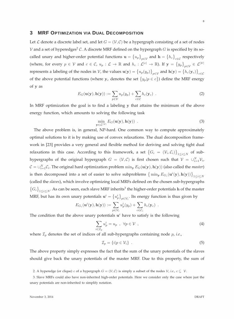
(b) General form of function f : X → Y in MRF/CRF training.(c)
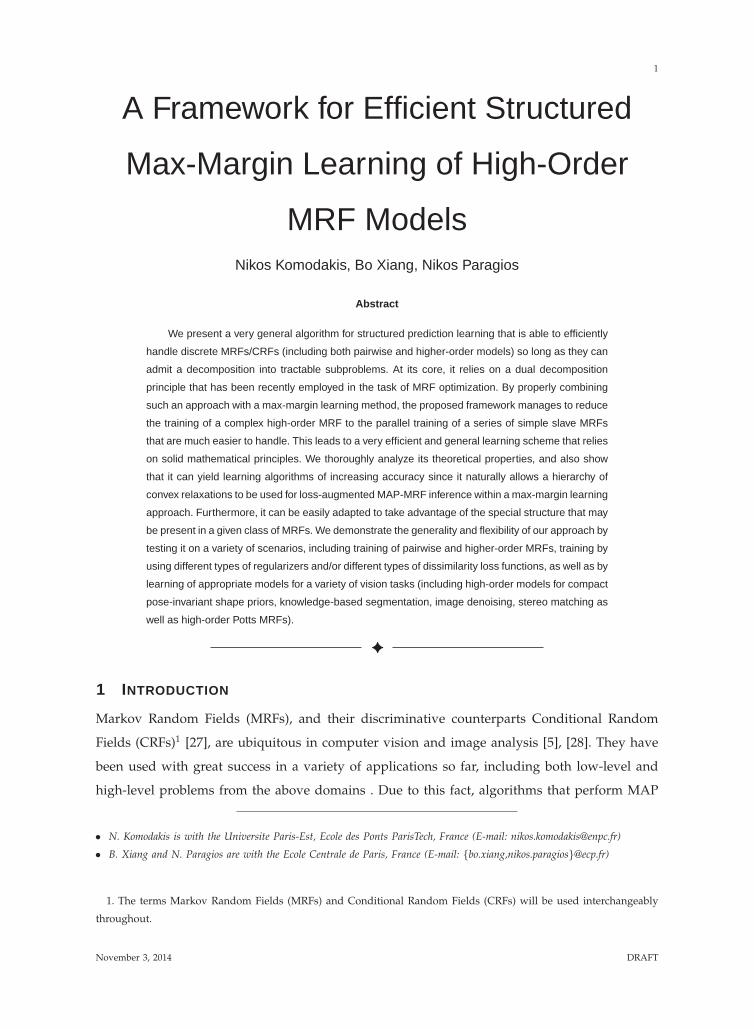
Fig. 1: (a) In MRF/CRF training, one aims to learn a mapping f : X → Y between a typically high-
dimensional input space X and an output space of MRF/CRF variables Y . In stereo matching, for instance,
the elements of the input space X correspond to stereoscopic images, and the elements of the output space
Y correspond to disparity maps. (b) In general, the mapping f(x) is defined as minimizing the energy
EG(u(y|w),h(y|w)) of an MRF/CRF model whose unary and higher-order potentials u(y|w), h(y|w)
are parameterized by w (the potentials also depend on x, but this is omitted here to simplify notation).
Therefore, to fully specify this mapping it suffices to estimate w, which is what parameter learning aims
to achieve in this case. (c) Our framework reduces, in a principled manner, the training of a complex
MRF model into the parallel training of a series of easy-to-handle slave MRFs. The latter can be freely
chosen so as to fully exploit the problem structure, which, in addition to efficiency, contributes a sufficient
amount of flexibility and generality to our method.
estimation for models of this type have attracted a significant amount of research interest in
the computer vision community over the past years [17], [48]. However, besides the ability to
accurately minimize the energy of a MRF model, another extremely crucial issue is how to
actually select this energy in the first place, such that the resulting model yields an accurate
representation of a specific problem that one aims to solve (a MAP-MRF solution is of little
value if the used MRF model does not properly represent the problem at hand). It turns out
that one of the most successful and principled ways for achieving this goal is through learning.
In such a context, one proceeds by parameterizing the potentials of a MRF model by a vector
of parameters w, and, then, these parameters are estimated automatically by making use of
training data that are given as input. For many cases in vision, this is, in fact, the only viable
solution as the existing parameters can often be too many to tune by hand (e.g., deformable
parts-based models for object detection can have thousands of parameters to estimate).
As a result, learning algorithms for MRF parameter estimation play a fundamental role
in successfully applying MRF models to computer vision problems. However, training these
models poses a task that is quite challenging. This is because, unlike standard machine learning
tasks where one must learn functions predicting simple true-false answers or scalar values (as
November 3, 2014 DRAFT
3
in classification and regression), the goal, in this case, is to learn models that predict answers
much more complex consisting of multiple interrelated variables. In fact, this is a characteristic
example of what is known as structured prediction learning, where one uses a set of input-output
training pairs{(xk,yk)
}1≤k≤K
⊆ X×Y to estimate a function f : X → Y that has the following
characteristics: both the input and output spaces X , Y are high-dimensional, and, furthermore,
the variables in Y are interrelated, i.e., each element y ∈ Y carries out some structure (for
instance, it can represent a graph). In the particular case of MRF parameter estimation, X is
representing the space where the observations (e.g., the input visual data) reside, whereas Y is
representing the space of the variables of the MRF model (see Fig. 1(a), 1(b)).
In fact, the difficulty of the above task becomes even greater due to the computational
challenges that are often raised by computer vision applications with regard to learning. For
instance, many of the MRFs used in vision are of large scale. Also, the complexity and diversity
of vision tasks often require the training of MRFs with complex potential functions. On top of
that, over the last years the use of high order MRFs is becoming increasingly popular in vision
since such MRFs are often found to considerably improve the quality of estimated solutions.
Yet, most of the MRF learning methods proposed in the vision literature so far focus mainly
on models with pairwise potentials or on specific classes of high-order models for which they
need to derive specifically tailored algorithms [1], [2], [25], [31], [34], [43], [49].
The goal of this work is to address the above mentioned challenges by proposing a general
learning method that can be directly applicable to a very broad class of problems. To achieve
this goal the proposed method makes use of some recent advances made on the MRF op-
timization side [22], [23], which it combines with a max-margin approach for learning [53].
More specifically, it makes use of a dual decomposition approach [23] that has been previously
used for MAP estimation. Thanks to this approach, it essentially manages to reduce the task
of training a complex MRF to that of training in parallel a series of simpler slave MRFs that
are much easier to handle within a max-margin framework (Fig. 1(c)). The concurrent training
of the slave MRFs takes place in a principled way through an efficient projected subgradient
algorithm. This leads to a powerful learning framework that makes the following contributions
compared to prior art:
1) It is able to efficiently handle not just pairwise log-linear MRF models but also high-order
ones as long as the latter can admit a decomposition into tractable subproblems, in which
case no other restriction needs to be imposed on the topology of the underlying MRF
graph or on the type of MRF potentials.
2) Thanks to the parallel training of a series of easy-to-handle submodels in combination with
the used projected subgradient method, it leads to a highly efficient learning scheme that
November 3, 2014 DRAFT
4
is scalable even to very large problems. Moreover, unlike prior cutting-plane or primal
subgradient descent methods for max-margin learning, which require performing loss-
augmented MAP-MRF inference to completion at every iteration, the proposed scheme
is able to jointly optimize both the vector of parameters and the loss-augmented MRF
inference variables.
3) It allows a hierarchy of convex relaxations for MAP-MRF estimation to be used in the con-
text of learning for structured prediction (where this hierarchy includes all the commonly
used LP relaxations for MRF inference), thus leading to structured prediction learning
algorithms of increasing accuracy.
4) It is sufficiently flexible and extendable, as it only requires providing a routine that
computes an optimizer for the slave MRFs. As a result, it can be easily adapted to take
advantage of the special structure that may exist in a given class of MRF models to be
trained.
The present paper is based on our previous work [19]. Compared to that work, here we also
provide a more detailed mathematical and theoretical analysis of our method as well as a
significantly extended set of experimental results, including results for learning pose invariant
models, for knowledge-basesd segmentation (both on 2D and 3D cases), for training using
high-order loss functions, as well as for training using sparsity inducing regularizers.
2 RELATED WORK
Over the past years, structured prediction learning has been a topic that has attracted a sig-
nificant amount of interest both from the vision and machine learning community. There is,
therefore, a substantial body of related work in this area.
Many approaches on this topic can essentially be derived from, or are based on, the so-
called regularized risk minimization paradigm, where one is given a set of training samples{(xk,yk)
}1≤k≤K
⊆ X×Y (assumed to be generated by some unknown distribution on X×Y )
and seeks to estimate the parameters w of a graphical model, such as a Markov Random Field,
by minimizing an objective function of the following form
minw
R(w) + C
K∑
k=1
L(yk, yk(xk|w)) . (1)
In the above, yk denotes the desired (i.e., ground truth) MRF labeling of the k-th training
sample, yk(xk|w) denotes the corresponding labeling that results from minimizing an MRF
instance constructed from the input xk and parameterized by w, and L(·, ·) is a loss func-
tion used for incurring a penalty if there exist differences between the two solutions yk and
November 3, 2014 DRAFT
5
yk(xk|w). In view of this notation, the second term in (1) represents essentially an empirical
risk that is used for approximating the true risk, which cannot be computed due to the fact
that the joint distribution on the input-output pairs (x,y) ∈ X × Y is not known. The above
approximation of the true risk is equal to the average of the loss on the input training samples,
which is combined in (1) with a regularizer R(w), whose main role is essentially to prevent
overfitting (the relative importance of the two terms, i.e., the regularizer and the empirical risk,
is determined by the regularization constant C in (1)).
Depending on the choice made for the loss function L(·, ·), different types of structured
prediction learning methods can be recovered, including both generative (e.g., maximum-
likelihood) and discriminative (e.g., max-margin) algorithms, which comprise the two most
general and widely used learning approaches. In the case of maximum-likelihood learning,
one maximizes (possibly along with an L2 norm regularization term) the product of posterior
probabilities of the ground truth MRF labelings∏
k P (yk|w), where P (y|w) ∝ exp(−E(y|w)
)
denotes the probability distribution induced by an MRF model with energy E(y|w). This
leads to a convex differentiable objective function that can be optimized using gradient ascent.
However, in the case of log-linear models, it is known that computing the gradient of this
function involves taking expectations (of some appropriate feature functions) with respect to
the MRF distribution P (y|w). This, therefore, requires performing probabilistic MRF inference,
which is, in general, an intractable task. As a result, approximate inference techniques (such
as the loopy belief propagation algorithm [35]) are often used for approximating the MRF
marginals required for the estimation of the gradient. This is, e.g., the case in [43], where
the authors demonstrate how to train a CRF model for stereo matching, as well as in [25],
where a comparison with other MRF training methods such as the pseudo-likelihood [4], [26]
and MCMC-based contrastive divergence [16] are included as well. A disadvantage, of course,
of having to use approximate probabilistic inference techniques is that the estimation of the
gradient is incorrect and so it is difficult for these methods to provide any theoretical guarantees.
Besides maximum-likelihood, another widely used class of structured prediction learning
techniques, the so-called max-margin learning methods, can be derived from (1) by choosing
a hinge-loss term as the loss function L(·, ·). In this case, it turns out that the goal of the
resulting optimization problem is to adjust the MRF parameters w so that, ideally, there is at
least a non-negative margin attained between the energy attained by the ground truth solution
of a training sample and the energy of any other solution.
When R(w) = ||w||2, such a problem is equivalent to a convex quadratic program (QP) with
an exponential number of linear inequality constraints. One class of methods [11], [29], [59] try
to solve this QP by use of a cutting-plane approach. These methods rely on the core idea that
November 3, 2014 DRAFT
6
only a very small fraction of the exponentially many constraints will actually be active at an
optimal solution. Therefore, they proceed by solving a small QP whose number of constraints
increases at each iteration. The increase, in this case, takes place by finding and adding the
most violated constraints each time (still, the total number of constraints can be shown to be
polynomially upper-bounded). However, one drawback of such an approach relates to the fact
that computing the most violated constraint requires solving at each iteration a loss-augmented
MAP-MRF inference problem that is, in general, NP-hard. Therefore, one still has to resort to
approximate MAP inference techniques. This can lead to the so-called under-generating or over-
generating approaches depending on the type of approximate inference used during this step.
The former approaches rely on algorithms that consider only a subset of all possible solutions
for the loss-augmented MAP-MRF inference step. As a consequence, solutions that are not
considered do not get penalized during training. In contrast, the latter approaches make use of
algorithms that consider a superset of the valid solutions. This typically means also penalizing
fractional solutions corresponding to a relaxation of the loss-augmented MAP-MRF inference
problem, thus promoting the extraction of a valid integral solution at test time. Due to this fact,
overgenerating approaches are typically found to have much better empirical performance [11].
Crucially, however, both undergenerating and overgenerating approaches typically impose
great computational cost during training, especially for problems of large scale or high order
that are frequently encountered in computer vision, due to the fact that the MAP inference
process has to be performed at the level of full size MRFs at each iteration. Note that this a
very important issue that appears in other existing methods as well, e.g., [41]. An exception
perhaps is the special case of submodular MRFs, for which the authors of [2] have shown
how to express the exponential set of constraints in a compact form, thus allowing for a more
efficient MRF training to take place under this setting.
The method proposed in this paper aims to address the aforementioned shortcomings. It
belongs to the class of overgenerating training methods. Among other methods of this type, the
approach closest to our work is [31], where the authors choose to replace the structured hinge-
loss for pairwise MRFs by a convex dual upper bound that decomposes over the MRF cliques
(the specific dual bound that has been used in this case is the one that was first employed in the
context of the max-sum diffusion algorithm [55]). That work, however, focuses on the training of
pairwise MRFs, but it can potentially be extended to higher-order models by properly adapting
the dual bound of [55] and deriving corresponding block-coordinate dual ascent methods.
Our method, on the other hand, handles directly in a unified, elegant and modular manner
high-order models, models that employ tighter relaxations for improved accuracy, higher-order
loss functions, as well as models with any type of special characteristics (e.g., submodularity).
November 3, 2014 DRAFT
7
Furthermore, [31] is theoretically valid, and thus applicable, only to problems with a strictly
convex regularizer such as the squared l2-norm. In contrast, our approach handles any convex
regularizer (including ones based on sparsity inducing norms - e.g., l1 - that have often proved
to be very useful during learning), offering guaranteed convergence in all cases. Moreover,
an additional advantage compared to [31] is that our method is parallelizable, as it allows all
of the optimizers for the slave MRFs to be computed concurrently (instead of sequentially).
One other max-margin training method that replaces the loss-augmented inference step by a
compact dual LP relaxation is the approach proposed in [12] . However, this is done only
for a restricted class of MRF problems (those with a strictly trivial equivalent), for which the
LP relaxation is assumed to be equivalent to the original MRF optimization. An additional
CRF learning method that makes use of duality is [15], which proposes an approximation for
the CRF structured-prediction problem based on a local entropy approximation and derives an
efficient message-passing algorithm with guaranteed convergence. Similarly to our method and
[31], the method proposed in [15] breaks down the classical separation between inference and
learning, and tries to directly formulate the learning problem via message passing operations,
but uses different dual formulations and optimization techniques.
It should be mentioned at this point that, over the last years, additional types of structured
prediction training methods have been proposed that can make use of various other types
of learning objective functions and losses, as well as optimization algorithms [9], [13], [30],
[32], [37], [39], [40], [50], [52]. This also includes recent cases such as the inference-machines
framework proposed in [33], as well as various types of randomized models such as the
“Perturb-and-MAP” framework [38] or the “randomized optimum models” described in [51].
Also, a pseudo-max approach to structured learning (inspired by the pseudo-likelihood method)
is proposed in [47], where the authors also analyze for which cases such an approach leads to
consistent training. Furthermore, learning algorithms that can handle graphical models with
hidden variables have been recently proposed as well, in which case it is assumed that only
partial ground truth labelings are given as input during training [10], [20], [24], [45], [60]. Last,
but not least, another strand of work focuses on developing learning approaches for the case
of continuously valued MRF problems [42].
The remainder of this paper is structured as follows. We begin by briefly reviewing the dual
decomposition method for MAP estimation in §3. We also review the max-margin structured
prediction approach in §4. We describe in detail our MRF learning framework and also thor-
oughly analyze various aspects of it in §5-§7. We show experimental results for a variety of
different settings and tasks in §8. Finally, we present our conclusions in §9.
November 3, 2014 DRAFT
8
3 MRF OPTIMIZATION VIA DUAL DECOMPOSITION
Let L denote a discrete label set, and let G = (V, C) be a hypergraph consisting of a set of nodes
V and a set of hyperedges2 C. A discrete MRF defined on the hypergraph G is specified by its so-
called unary and higher-order potential functions u ={up
}p∈V
and h ={hc
}c∈C
respectively
(where, for every p ∈ V and c ∈ C, up : L → R and hc : L|c| → R). If y ={yp}p∈V∈ L|V|
represents a labeling of the nodes in V , the values u(y) ={up(yp)
}p∈V
and h(y) ={hc(yc)
}c∈C
of the above potential functions (where yc denotes the set{yp|p ∈ c
}) define the MRF energy
of y as
EG(u(y),h(y)) :=∑
p∈V
up(yp) +∑
c∈C
hc(yc) . (2)
In MRF optimization the goal is to find a labeling y that attains the minimum of the above
energy function, which amounts to solving the following task
miny∈L|V|
EG(u(y),h(y)) . (3)
The above problem is, in general, NP-hard. One common way to compute approximately
optimal solutions to it is by making use of convex relaxations. The dual decomposition frame-
work in [23] provides a very general and flexible method for deriving and solving tight dual
relaxations in this case. According to this framework, a set{Gi = (Vi, Ci)
}1≤i≤N
of sub-
hypergraphs of the original hypergraph G = (V, C) is first chosen such that V = ∪Ni=1Vi,
C = ∪Ni=1Ci. The original hard optimization problem miny EG(u(y),h(y)) (also called the master)
is then decomposed into a set of easier to solve subproblems{miny EGi
(ui(y),h(y))}1≤i≤N
(called the slaves), which involve optimizing local MRFs defined on the chosen sub-hypergraphs{Gi
}1≤i≤N
. As can be seen, each slave MRF inherits3 the higher-order potentials h of the master
MRF, but has its own unary potentials ui ={uip
}p∈Vi
. Its energy function is thus given by
EGi(ui(y),h(y)) :=
∑
p∈Vi
uip(yp) +
∑
c∈Ci
hc(yc) .
The condition that the above unary potentials ui have to satisfy is the following∑
i∈Ip
uip = up , ∀p ∈ V , (4)
where Ip denotes the set of indices of all sub-hypergraphs containing node p, i.e.,
Ip = {i|p ∈ Vi} . (5)
The above property simply expresses the fact that the sum of the unary potentials of the slaves
should give back the unary potentials of the master MRF. Due to this property, the sum of
2. A hyperedge (or clique) c of a hypergraph G = (V, C) is simply a subset of the nodes V , i.e., c ⊆ V .
3. Slave MRFs could also have non-inherited high-order potentials. Here we consider only the case where just the
unary potentials are non-inherited to simplify notation.
November 3, 2014 DRAFT

9
the minimum energies of the slaves can be shown to always provide a lower bound to the
minimum energy of the master MRF, i.e., it holdsN∑
i=1
miny
EGi(ui(y),h(y)) ≤ min
yEG(u(y),h(y)) . (6)
Maximizing the lower bound appearing on the left-hand side of (6) by adjusting the unary
potentials{ui}1≤i≤N
(which play the role of dual variables in this case) gives rise to the
following dual relaxation for problem (3)
DUAL{Gi
}(u,h) = max{ui}1≤i≤N
N∑
i=1
miny
EGi(ui(y),h(y)) (7)
s.t.∑
i∈Ip
uip = up , (∀p ∈ V) . (8)
By simply choosing different decompositions{Gi
}1≤i≤N
of the hypergraph G, one can derive
different convex relaxations to problem (3). These include the standard marginal polytope LP
relaxation for pairwise MRFs, which is widely used in practice, as well as alternative relaxations
that can be much tighter4.
4 MAX-MARGIN MARKOV NETWORKS
Let us now return to the central topic of the paper, which is the training of MRF/CRF models.
To that end, let{xk,yk
}1≤k≤K
∈ X×Y be a training set of K samples, where xk, yk represent
the input observations and the label assignments of the k-th sample, respectively. We assume
that the MRF instance associated with the k-th sample is defined on a hypergraph5 G = (V, C),
and both the unary potentials uk ={ukp
}p∈V
and the higher-order potentials hk ={hkc
}c∈C
of
that MRF are parameterized linearly in terms of a vector of parameters w we seek to estimate,
i.e.,
ukp(yp|w) = wT · φp(yp,x
k), hkc (yc|w) = wT · φc(yc,x
k) , (9)
where φp(·, ·), φc(·, ·) represent known vector-valued feature functions that are extracted from
the corresponding observations xk (and are application-specific). Note that, by properly zero-
padding these vector-valued features φp(·, ·) and φc(·, ·), the above formulation allows us to
use separate parameters for each different node, clique or even label6.
4. We should note, though, that none of these relaxations are guaranteed to be exact in the general case.
5. In general, each MRF training instance can be defined on a different hypergraph Gk = (Vk, Ck), but here we
assume Gk = G, ∀k in order to reduce notation clutter.
6. For instance, if ukp(yp|w) = wT
p,yp· φp(yp,xk) and hk
c (yc|w) = wTc,yc· φc(yc,x
k), we can define w as the
concatenation of all vectors{wp,yp
}and
{wc,yc
}, in which case each feature vector φp(yp,xk) should be defined as
a properly zero-padded extension of φp(yp,xk) that has the same size as w (and similarly for φc(yc,xk)).
November 3, 2014 DRAFT
10
Let ∆(y,y′) represents a dissimilarity measure between any two MRF labelings y and y′
(that satisfies ∆(y,y′) ≥ 0 and ∆(y,y) = 0). In a maximum margin Markov network [53] one
ideally seeks a vector of parameters w such that the MRF energy of the desired ground-truth
solution yk is smaller by a margin ∆(y,yk) than the MRF energy of any other solution y, i.e.,
(∀y), EG(uk(yk|w),hk(yk|w)) ≤ EG(u
k(y|w),hk(y|w))−∆(y,yk) . (10)
To account for the fact that there might be no vector w satisfying all of the above constraints,
a slack variable ξk per sample is introduced that allows some of the constraints to be violated
(∀y), EG(uk(yk|w),hk(yk|w)) ≤ EG(u
k(y|w),hk(y|w))−∆(y,yk) + ξk . (11)
Ideally, ξk should take a zero value. In general, however, it can hold ξk > 0 and so the goal,
in this case, is to adjust w such that the sum∑K
k=1 ξk (which represents the total violation of
constraints (10)) takes a value that is as small as possible. This leads to solving the following
constrained minimization problem, where a regularization term R(w) has been also added so
as to prevent the components of w from taking too large values
minw
R(w) + C
K∑
k=1
ξk (12)
s.t. ξk ≥ EG(uk(yk|w),hk(yk|w))−
(EG(u
k(y|w),hk(y|w))−∆(y,yk)), (∀y) (13)
The term R(w) can be chosen in several different ways (for instance, it is often set as a squared
Euclidean norm 12||w||2, or as a sparsity inducing norm like||w||1).
It is easy to see that at an optimal solution of problem (12) each variable ξk should equal to
ξk = EG(uk(yk|w),hk(yk|w))−min
y
(EG(u
k(y|w),hk(y|w))−∆(y,yk)). (14)
Furthermore, assuming that the dissimilarity measure ∆(y,yk) decomposes in the same way
as the MRF energy, i.e., it holds
∆(y,yk) =∑
p∈V
δp(yp, ykp ) +
∑
c∈C
δc(yc,ykc ) , (15)
we can define the following loss-augmented MRF potentials uk(y|w), hk(y|w)
ukp(· |w) = uk
p(· |w)− δp(· , ykp ) (16)
hkc (· |w) = hk
c (· |w)− δc(· ,ykc ) , (17)
which allow expressing the slack variable in (14) as ξk = LkG(w), with Lk
G(w) being defined as
the following hinge loss term
LkG(w) := EG(u
k(yk|w), hk(yk|w))−miny
EG(uk(y|w), hk(y|w)) . (18)
Therefore, problem (12) finally reduces to the following unconstrained optimization task
minw
R(w) + CK∑
k=1
LkG(w) , (19)
November 3, 2014 DRAFT
11
which shows that maximum-margin learning essentially corresponds to using the hinge loss
term LkG(w) as the loss L(yk, yk(w)) in the empirical minimization task (1). Intuitively, this
term LkG(w) expresses the fact that the loss will be zero only when the loss-augmented MRF
with potentials uk, hk attains its minimum energy at the desired solution yk.
5 LEARNING VIA DUAL DECOMPOSITION
Unfortunately, even evaluating (let alone minimizing) the loss function LkG(w) is going to be in-
tractable in general. This is because it is NP-hard to compute the term miny EG(uk(y|w), hk(y|w))
involved in the definition of LkG(w) in (18). To address this fundamental difficulty, here we
propose to approximate the above term (that involves computing the optimum energy of a
loss-augmented MRF with potentials uk, hk) with the corresponding optimum of a convex
relaxation DUAL{Gi
}(uk, hk) that is derived based on dual decomposition.
To accomplish that, as explained in section 3, we must first choose an arbitrary decomposition
of the hypergraph G = (V, C) into sub-hypergraphs {Gi = (Vi, Ci)}1≤i≤N . Then, for the k-th
training sample and for each sub-hypergraph Gi, we define a slave MRF on Gi that has its own
unary potentials uk,i while inheriting the higher-order potentials hk. These slave MRFs are used
for approximating miny EG(uk(y|w), hk(y|w)) (i.e., the minimum energy of the loss-augmented
MRF of the k-th training sample) with the following convex relaxation DUAL{Gi
}(uk, hk)
DUAL{Gi
}(uk, hk) = max{uk,i}1≤i≤N
N∑
i=1
miny
EGi(uk,i(y), hk(y|w)) (20)
s.t.∑
i: p∈Vi
uk,ip = uk
p , (∀p ∈ V). (21)
If we now replace in (18) the optimum miny EG(uk(y|w), hk(y|w)) with the optimum of the
above convex relaxation DUAL{Gi
}(uk, hk), we get the following derivation
LkG(w) = EG(u
k(yk|w), hk(yk|w))−miny
EG(uk(y|w), hk(y|w)) (22)
≈ EG(uk(yk|w), hk(yk|w))−DUAL{
Gi
}(uk, hk) (23)
= EG(uk(yk|w), hk(yk|w))− max
{uk,i}1≤i≤N
N∑
i=1
miny
EGi(uk,i(y), hk(y|w)) (24)
= min{uk,i}1≤i≤N
(EG(u
k(yk|w), hk(yk|w))−N∑
i=1
miny
EGi(uk,i(y), hk(y|w))
), (25)
where in (25) we have made use of the following identity that holds for any function f
− max{uk,i}1≤i≤N
f({uk,i}) = min{uk,i}1≤i≤N
(− f({uk,i})) .
Due to the fact that the dual variables uk,i have to satisfy constraint (21), i.e., ukp =
∑i: p∈Vi
uk,ip ,
November 3, 2014 DRAFT
12
the following equality stands in this case
EG(uk(yk|w), hk(yk|w)) =
N∑
i=1
EGi(uk,i(yk), hk(yk|w)) . (26)
By substituting this equality into (25), we finally get
LkG(w) ≈ min
{uk,i}1≤i≤N
N∑
i=1
(EGi
(uk,i(yk), hk(yk|w))− miny
EGi(uk,i(y), hk(y|w))
). (27)
Therefore, if we define
LkGi(w,uk,i) := EGi
(uk,i(yk), hk(yk|w))− miny
EGi(uk,i(y), hk(y|w)) (28)
equation (27) translates into
LkG(w) ≈ min
{uk,i}1≤i≤N
∑
i
LkGi(w,uk,i) . (29)
Note that each LkGi(w,uk,i) corresponds to a hinge loss term that is exactly similar to Lk
G(w)
except from the fact that the former relates to a slave MRF on Gi with potentials uk,i, hk,
whereas the latter relates to an MRF on G with potentials uk, hk.
The final function to be minimized results from substituting (29) into (19), thus leading to
the following optimization problem
minw,{uk,i}1≤k≤K,1≤i≤N
R(w) + C
K∑
k=1
N∑
i=1
LkGi(w,uk,i) (30)
s.t.∑
i: p∈Vi
uk,ip = uk
p , (∀k ∈ {1, 2, . . . ,K}, p ∈ V). (31)
As can be seen, the initial objective function (19) (which was intractable due to containing the
hinge losses LkG(·)) has now been decomposed into the hinge losses Lk
Gi(·) that are a lot easier
to handle.
If a projected subgradient method [3] is used for minimizing the resulting convex function, we
get algorithm 1, for which the following theorem holds true:
Theorem 1. If multipliers αt ≥ 0 satisfy limt→∞ αt = 0,∑∞
t=0 αt = ∞, then, the iterative updates
in Algorithm 1 converge to an optimal solution of problem (30).
Proof: We are going to make use of the following auxiliary variables λk,i = {λk,i
p }p∈Vi,
which are defined in terms of the variables uk,i = {uk,ip }p∈Vi
as follows
λk,ip = uk,i
p −ukp
|Ip|, (32)
where 1 ≤ k ≤ K, 1 ≤ i ≤ N , and Ip = {i|p ∈ Vi}. In this case, constraints (31) map into
constraints {λk,i}1≤k≤K,1≤i≤N ∈ Λ, where the set Λ is given by
Λ =
{{λk,i}1≤k≤K,1≤i≤N
|∑
i∈Ip
λk,ip = 0
}. (33)
To prove the theorem, we will proceed by showing that Algorithm 1 corresponds to applying
the projected subgradient method to problem (30) with respect to variables w, {λk,i}1≤k≤K,1≤i≤N .
November 3, 2014 DRAFT
13
According to the projected subgradient method, variables w,{λk,i}1≤k≤K,1≤i≤N
must be up-
dated at each iteration using the following scheme [3], [46]
w← w − αt · dw (34)
λk,i ← ProjΛ(λ
k,i − αt · dλk,i) . (35)
In the above, dw and{dλk,i
}1≤k≤K,1≤i≤N
denote the components of a subgradient of the
objective function (30) (with respect to w and{λk,i}1≤k≤K,1≤i≤N
, respectively), and ProjΛ(·)
denotes projection onto the feasible set Λ.
To compute these components, a subgradient of function LkGi(w,uk,i) must be computed
first, which in turns requires computing a subgradient of the term −miny EGi(uk,i(y), hk(y|w)),
which is the only non-differentiable term used in the definition of LkGi(w,uk,i). This can be
done by making use of the following well known lemma7
Lemma. Let f(x) = maxm=1,...,M fm(x), with fm being convex and differentiable functions of x. A
subgradient of f at x0 is given by ∇fm(x0), where m = argmaxm fm(x0).
Based on the above lemma, a subgradient of the term −miny EGi(uk,i(y), hk(y|w)) is given
by the gradient vector −∇EGi(uk,i(yk,i), hk(yk,i|w)), where yk,i denotes a minimizer for the
energy EGi(uk,i(y), hk(y|w)) of the slave MRF defined on sub-hypergraph Gi. This gradient
vector has the following components:
−∂EGi
(uk,i(yk,i), hk(yk,i|w))
∂w= −
∂
∂w
∑
p∈Vi
uk,ip (yk,ip ) +
∑
c∈Ci
hkc (y
k,ic |w)
(32)= −
∂
∂w
∑
p∈Vi
(ukp(y
k,ip |w)
|Ip|+ λk,i
p (yk,ip )
)+∑
c∈Ci
hkc (y
k,ic |w)
= −∂
∂w
∑
p∈Vi
ukp(y
k,ip |w)
|Ip|+∑
c∈Ci
hkc (y
k,ic |w)
(9)= −
∑
p∈Vi
φp(yk,ip ,xk)
|Ip|−∑
c∈Ci
φc(yk,ic ,xk) ,
−∂EGi
(uk,i(yk,i), hk(yk,i|w))
∂λk,ip (l)
= −∂EGi
(uk,i(yk,i), hk(yk,i|w))
∂uk,ip (l)
·∂uk,i
p (l)
∂λk,ip (l)
= −∂uk,i
p (yk,ip )
∂uk,ip (l)
·∂uk,i
p (l)
∂λk,ip (l)
(32)= −
∂uk,ip (yk,ip )
∂uk,ip (l)
= −[yk,ip = l
],
where [ · ] denotes the Iverson bracket, i.e., it equals 1 if the expression in square brackets is
satisfied, and 0 otherwise. Based on the above result, it is easy to verify that the components
7. The proof of this lemma follows from the fact that f(x) ≥ fm(x) ≥ fm(x0) + ∇fm(x0)⊤(x− x0) = f(x0) +
∇fm(x0)⊤(x− x0).
November 3, 2014 DRAFT

14
dw,{dλk,i
}1≤k≤K,1≤i≤N
of a total subgradient of the objective function (30) are given by
dw = ∇R(w) + C
∑
k,i,p
φp(ykp ,x
k)− φp(yk,ip ,xk)
|Ip|+∑
k,i,c
(φc(y
kc ,x
k)− φc(yk,ic ,xk)
) (36)
dλk,ip (l) = C
([ykp = l
]−[yk,ip = l
]). (37)
Furthermore, after the update λk,i ← λ
k,i−αt·dλk,i, eq. (35) also requires projecting the resulting
λk,i onto the feasible set Λ. This projection is equivalent to subtracting
(∑i∈Ip
λk,ip
)/|Ip| from
each λk,ip such that the sum
∑i∈Ip
λk,ip remains equal to zero as required by the definition of
Λ. Based on this observation and the definition of dλk,i given in eq. (37), the combined update
(35) reduces to
λk,ip (l) += αtC
([yk,ip = l
]−
∑j∈Ip
[yk,jp = l
]
|Ip|
). (38)
All the above lead to the pseudocode of algorithm 1.
The proof now follows directly from the fact that the subgradient updates are known to
converge to an optimal solution if the multipliers αt satisfy the conditions stated in the theorem
(see Proposition 2.2 in [36]). Interestingly, the key quantity to proving the convergence of the
subgradient method is not the objective function value (which may have temporary fluctua-
tions), but the Euclidean distance to an optimal solution, which is guaranteed to decrease per
iteration. The proof of this is based on the fact that the angle between the current subgradient
and the vector formed by the difference of the current iterate with an optimal solution is less
than 90 degrees.
Let us pause for a moment to see what we have been able to accomplish so far. Comparing
objective functions (19) and (30), we can immediately see that, thanks to the use of dual
decomposition, we have managed to replace each term LkG, which is the hinge loss of a possibly
difficult-to-solve high-order MRF on G, with the sum of the terms{LkGi
}1≤i≤N
that are the
hinge losses of a series of simpler slave MRFs on sub-hypergraphs{Gk
i
}1≤i≤N
. In this manner,
we have essentially been able to reduce the difficult task of training a complex high-order MRF
to the much easier task of training in parallel a series of simpler slave MRFs.
At a high level, to achieve this goal, the resulting learning algorithm operates by allowing
each slave MRF to have its own unary potentials uk,i and by properly adjusting these potentials
such that the estimated minimizer yk,i of each slave MRF coincides with the desired ground
truth solution yk restricted on the nodes of Gi. This is essentially done via updates (38) and
(34). To get a better intuition for the role of these updates, note that the aim of the former
updates is to modify uk,i such that the minimizers of different slave MRFs are consistent with
each other (i.e., they agree for the labels that are assigned to common nodes). Indeed, it is easy
to verify that the right hand side of (38) equals to zero (which means that, as a result of this
November 3, 2014 DRAFT
15
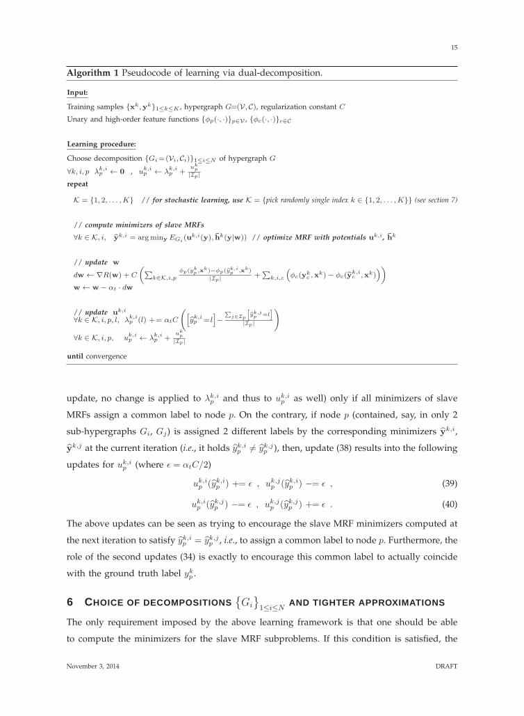
Algorithm 1 Pseudocode of learning via dual-decomposition.
Input:
Training samples {xk,yk}1≤k≤K , hypergraph G=(V, C), regularization constant C
Unary and high-order feature functions {φp(·, ·)}p∈V , {φc(·, ·)}c∈C
Learning procedure:
Choose decomposition {Gi=(Vi, Ci)}1≤i≤N of hypergraph G
∀k, i, p λk,ip ← 0 , u
k,ip ← λ
k,ip +
ukp
|Ip|
repeat
K = {1, 2, . . . ,K} // for stochastic learning, use K = {pick randomly single index k ∈ {1, 2, . . . ,K}} (see section 7)
// compute minimizers of slave MRFs
∀k ∈ K, i, yk,i = argminy EGi(uk,i(y), hk(y|w)) // optimize MRF with potentials uk,i, hk
// update w
dw← ∇R(w) + C
(∑k∈K,i,p
φp(ykp ,xk)−φp(y
k,ip ,xk)
|Ip|+∑
k,i,c
(φc(yk
c ,xk)− φc(y
k,ic ,xk)
))
w← w − αt · dw
// update uk,i
∀k ∈ K, i, p, l, λk,ip (l) += αtC
([yk,ip = l
]−
∑j∈Ip
[yk,jp =l
]
|Ip|
)
∀k ∈ K, i, p, uk,ip ← λ
k,ip +
ukp
|Ip|
until convergence
update, no change is applied to λk,ip and thus to uk,i
p as well) only if all minimizers of slave
MRFs assign a common label to node p. On the contrary, if node p (contained, say, in only 2
sub-hypergraphs Gi, Gj) is assigned 2 different labels by the corresponding minimizers yk,i,
yk,j at the current iteration (i.e., it holds yk,ip 6= yk,jp ), then, update (38) results into the following
updates for uk,ip (where ǫ = αtC/2)
uk,ip (yk,ip ) += ǫ , uk,j
p (yk,ip ) −= ǫ , (39)
uk,ip (yk,jp ) −= ǫ , uk,j
p (yk,jp ) += ǫ . (40)
The above updates can be seen as trying to encourage the slave MRF minimizers computed at
the next iteration to satisfy yk,ip = yk,jp , i.e., to assign a common label to node p. Furthermore, the
role of the second updates (34) is exactly to encourage this common label to actually coincide
with the ground truth label ykp .
6 CHOICE OF DECOMPOSITIONS{Gi
}1≤i≤N
AND TIGHTER APPROXIMATIONS
The only requirement imposed by the above learning framework is that one should be able
to compute the minimizers for the slave MRF subproblems. If this condition is satisfied, the
November 3, 2014 DRAFT
16
previously described algorithm can automatically take care of the entire MRF training process.
As a result of this fact, the proposed framework provides a great amount of flexibility. For
instance, a user is freely allowed to utilize different decompositions{Gi
}1≤i≤N
. As we will
explain next, this fact can be utilized for improving the learning algorithm in various ways.
To that end, let F0 denote the minimum of the original regularized loss function (19) and let
F{Gi
} denote the minimum of loss function (30) that results from using decomposition{Gi
}.
The following theorem holds true
Theorem 2. Loss F{Gi} upper bounds F0, i.e., F0 ≤ F{Gi}
Proof: By definition (19) it holds that
F0 =minw
R(w) + C
K∑
k=1
LkG(w)
(18)= min
wR(w) + C
K∑
k=1
(EG(u
k(yk|w), hk(yk|w))−miny
EG(uk(y|w), hk(y|w))
)(41)
≤minw
R(w) + CK∑
k=1
(EG(u
k(yk|w), hk(yk|w))−DUAL{Gi
}(uk, hk)
)(42)
=minw
R(w) + CK∑
k=1
(EG(u
k(yk|w), hk(yk|w))− max{uk,i}1≤i≤N
N∑
i=1
miny
EGi(uk,i(y), hk(y|w))
)
=minw
R(w) + C
K∑
k=1
min{uk,i}1≤i≤N
(EG(u
k(yk|w), hk(yk|w))−N∑
i=1
miny
EGi(uk,i(y), hk(y|w))
)
= minw,{uk,i}1≤k≤K,1≤i≤N
R(w) + C
K∑
k=1
N∑
i=1
(EGi
(uk,i(yk), hk(yk|w))−miny
EGi(uk,i(y), hk(y|w))
)
(43)
= minw,{uk,i}1≤k≤K,1≤i≤N
R(w) + CK∑
k=1
N∑
i=1
LkGi(w,uk,i) = F{Gi} , (44)
where inequality (42) is true because DUAL{Gi
}(uk, hk) is a convex relaxation of problem
miny EG(uk(y|w), hk(y|w)), while equality (43) is satisfied due to that EG(u
k(yk|w), hk(yk|w)) =∑N
i=1 EGi(uk,i(yk), hk(yk|w)) since
∑i∈Ip
uk,ip = uk
p .
The above theorem implies that, by minimizing F{Gi
}, one can also guarantee that the orig-
inal loss F0 will decrease as well. Not only that but, by appropriately choosing the hypergraph
decomposition{Gi
}, we can also improve the approximation F{
Gi
} to the true loss F0. This is
true because the tightness of the convex relaxation DUAL{Gi
} depends crucially on the choice
of decomposition{Gi
}. More specifically, we will say that decomposition
{Gj
}is stronger than
decomposition{Gi
}(and we will denote this by
{Gi
}<{Gj
}) if the convex relaxation from
{Gj
}is tighter than the relaxation from
{Gi
}, i.e., it always holds DUAL{
Gi
} <DUAL{Gj
}.
November 3, 2014 DRAFT
17
Under this notation, the following theorem is true
Theorem 3. If{Gi
}<{Gj
}then F0≤F{
Gj
}<F{Gi
}, i.e., F{Gj
} is a better approximation to F0
than F{Gi
}.
Proof: By definition (30) it holds that
F{Gi
} = minw,{uk,i}1≤k≤K,1≤i≤N
R(w) + CK∑
k=1
N∑
i=1
LkGi(w,uk,i) (45)
=minw
R(w) + CK∑
k=1
(EG(u
k(yk|w), hk(yk|w))−DUAL{Gi
}(uk, hk)
), (46)
where the equality (46) is derived using a similar reasoning as in the proof of theorem 2 above.
Similarly, the following equality can be shown to hold true
F{Gj}=min
wR(w) + C
K∑
k=1
(EG(u
k(yk|w), hk(yk|w))−DUAL{Gj
}(uk, hk)
). (47)
By assumption it also holds{Gi
}<{Gj
}, which means that the relaxation DUAL{
Gj
}(uk, hk)
is tighter than the relaxation DUAL{Gi
}(uk, hk), which in turn implies that
DUAL{Gi
}(uk, hk) < DUAL{Gj
}(uk, hk) . (48)
The theorem now follows directly by combining equations (46), (47) and (48).
Given any MRF graph, it is always possible to choose a decomposition Gsingle ={Gc
}c∈C
,
which contains a sub-hypergraph Gc = (Vc, Cc) for each clique c ∈ C where Vc = {p|p ∈ c}
and Cc = {c}. In this case, each slave MRF consists of a single high-order clique. Due to this
fact, such slaves are often very easy to optimize regardless of the complexity of the original
MRF. As a result, the derived learning algorithm can have wide applicability. Furthermore, the
convex relaxation DUALGsingle(uk, hk) resulting from Gsingle can be shown to coincide with the
LP relaxation of the following integer programming formulation of MRF optimization [21]:
minz
∑
p
∑
yp
ukp(yp|w)zp(yp) +
∑
c
∑
yc
hkc (yc|w)zc(yc) (49)
s.t.∑
yp
zp(yp) = 1 , ∀p ∈ V (50)
∑yc:yp=l
zc(yc) = zp(l) , ∀c ∈ C, p ∈ c, l ∈ L (51)
zp(·), zc(·) ∈ {0, 1} , (52)
In the above, zp(yp) and zc(yc) are binary indicator variables that exist respectively for each
label yp of node p and each labeling yc of clique c. Note that such a relaxation extends the
marginal polytope relaxation [7], [44], which is commonly used for pairwise MRFs, to the case
of higher-order MRF models.
Of course, one can also choose decompositions{Gj
}that are stronger than Gsingle. Based
November 3, 2014 DRAFT

18
on theorem 3 above, this can lead to using better approximations of the loss F0 . This can be
achieved, for instance, by taking advantage of the special structure that may exist in certain
classes of MRFs. One characteristic example appears in [21] for the case of MRFs with the
so-called pattern-based potentials. More generally, the following theorem holds true:
Theorem 4. F{Gj
} is a better approximation to F0 than FGsingleonly if decomposition
{Gj
}1≤j≤N
has at least one sub-hypergraph Gj for which slave MRFs on Gj do not have the integrality property8.
Proof: As mentioned above, the MRF optimization problem miny EG(uk(y|w), hk(y|w)) can
be equivalently formulated as the following linear integer program:
minz
∑
p∈V
∑
yp
ukp(yp|w)zp(yp) +
∑
c∈C
∑
yc
hkc (yc|w)zc(yc) (53)
s.t z ∈ Z(G) , (54)
where the feasible set Z(G) is defined for any hypergraph G = (V, C) as follows
Z(G) ={z ∈ Z(G) | zp(·), zc(·) ∈ {0, 1}, ∀ p ∈ V, c ∈ C
}, (55)
Z(G) =
z
∣∣∣∣∣∣∣∣∣∣∣∣
∑yp
zp(yp) = 1, ∀ p ∈ V
∑yc:yp=l
zc(yc) = zp(l), ∀ c ∈ C, p ∈ c, l ∈ L
zp(·) ≥ 0, zc(·) ≥ 0, ∀ p ∈ V, c ∈ C
.
Let{Gj = (Vj , Cj)
}1≤j≤N
be a hypergraph decomposition of G (i.e. ∪Nj=1Vj = V , ∪Nj=1Cj = C,
Cj ∩ Cj′ = ∅, ∀j 6= j′) and let {uk,j}1≤j≤N be the corresponding set of unary potentials for the
slave MRFs of the k-th training sample, which satisfy equation (31), i.e.∑
j∈Ip
uk,jp = uk
p, (56)
where Ip = {j|p ∈ Vj} (e.g. uk,j can be chosen as uk,jp = uk
p/|Ip|). Using these potentials, the
above linear integer program (53) can be equivalently expressed as
minz,{zj}1≤j≤N
N∑
j=1
∑
p∈Vj
∑
yp
uk,jp (yp)z
jp(yp) +
∑
c∈Cj
∑
yc
hkc (yc|w)zjc(yc)
(57)
s.t. zj ∈ Z(Gj) , ∀j ∈ {1, 2, . . . , N} (58)
zjp = zp , ∀j ∈ {1, 2, . . . , N}, p ∈ V . (59)
The convex relaxation DUAL{Gj
}(uk, hk) is derived by relaxing constraints (59) and then
solving the resulting Lagrangian relaxation. Therefore, DUAL{Gj
}(uk, hk) results from the
8. We say that an MRF has the integrality property if and only if the corresponding LP relaxation of (49) is tight.
November 3, 2014 DRAFT
19
above problem (57) by simply replacing constraints (59) with the constraints zj ∈ CH(Z(Gj)
),
where CH(·) denotes the convex hull of a set.
If we now assume that all slave MRFs corresponding to decomposition{Gj
}have the
integrality property then, by definition, this implies that CH(Z(Gj)
)= Z(Gj) (i.e. we can
safely ignore the integrality constraints in (55)) and so DUAL{Gj
}(uk, hk) further reduces to
minz,{zj}1≤j≤N
N∑
j=1
∑
p∈Vj
∑
yp
uk,jp (yp)z
jp(yp) +
∑
c∈Cj
∑
yc
hkc (yc|w)zjc(yc)
(60)
s.t. zj ∈ Z(Gj) , ∀j ∈ {1, 2, . . . , N} (61)
zjp = zp , ∀j ∈ {1, 2, . . . , N}, p ∈ V . (62)
Due to constraints (56) and (62), the objective function (60) above is equal to the objective
function (49). Furthermore, constraints (61) are equivalent to constraints (54) after the integrality
constraints in the latter have been replaced by non-negativity constraints on the z variables.
Therefore, problem (60) is equivalent to the LP relaxation of the linear integer program (49),
which, as mentioned earlier, corresponds to the dual relaxation derived from decomposition
Gsingle. This concludes the proof of the theorem.
Based on the above theorem, one can, for instance, provably derive better learning algorithms
for pairwise MRF models just by using decompositions containing loopy subgraphs of small
tree width (MRFs on such subgraphs can still be efficiently optimized via, e.g., the junction tree
algorithm).
However, besides improving the accuracy of a learning algorithm, an appropriate choice of
a decomposition{Gi
}can also improve the computational efficiency of that algorithm. For
instance, consider the case of pairwise MRFs and a decomposition Gtree ={Ti
}that consists
entirely of spanning trees Ti of an MRF graph G. Although in this case the accuracy of learning
is not improved compared to Gsingle (due to the fact that it holds DUALGtree= DUALGsingle
and thus FGtree= FGsingle
[23]), the speed of convergence does improve in practice. The reason
is because, when using convex relaxation DUALGtree, each slave MRF now covers a much
larger number of nodes, which allows information to propagate faster across the whole graph
G during the MRF dual decomposition updates.
More generally, computational efficiency can be significantly improved simply by choosing
a decomposition that is specifically adapted to the class of MRFs we aim to train. For instance,
if part of the energy of a MRF is known to be submodular we can take advantage of this fact
simply by using that part as a slave. The very fast graph-cut based optimizers that exist for
submodular energies can be used directly and will greatly reduce the computational cost of
learning in this case.
November 3, 2014 DRAFT
20
7 INCREMENTAL AND STOCHASTIC SUBGRADIENT
To further improve computational efficiency we can also use an incremental subgradient method,
which is well suited to objective functions that can be expressed as a sum of components, like
in the case of objective function (30) that is given by R(·)+C∑K
k=1
∑N
i=1 LkGi(·), where K is the
number of training samples and N the number of sub-hypergraphs in the decomposition. At
each iteration of the incremental subgradient method, a step is taken along the subgradient
of only one component, where this component can be picked either deterministically (by
repeatedly visiting all components in a fixed order) or uniformly at random. A component
for the above objective function can have the following form:
R(·) + C∑
i∈S
LkGi(·) ,
where S denotes a subset of the set {1, 2, . . . , N}. In other words, at each iteration we need to
consider the hinge losses LkGi(·) for only a subset of slave MRFs corresponding to the indices
in S (in this case updates are similar to (38), (34) but they need to take into account only a
subset of slaves).
For instance, when using a randomized version of this scheme, we can decide to pick at
each iteration the index of a training sample k randomly from {1, . . . ,K}, and then also pick a
subset S randomly from a predefined partition of the slave indices of the k-th sample. If S is
always chosen to contain all slave indices of the k-th sample then this is essentially equivalent
to the more well known stochastic subgradient algorithm, in which case the total subgradient
with respect to w is computed analogously to (36) as follows
dw = ∇R(w) + C
∑
i,p
φp(ykp ,x
k)− φp(yk,ip ,xk)
|Ip|+∑
i,c
(φc(y
kc ,x
k)− φc(yk,ic ,xk)
) . (63)
To implement this learning scheme, we can modify Algorithm 1 by simply choosing K as a
randomly picked index from {1, 2, . . . ,K} at each iteration. Just like the subgradient method,
the resulting algorithm is guaranteed to converge to an optimal solution since a theorem similar
to Thm. 1 is known to also hold true for the incremental subgradient method [36].
8 EXPERIMENTAL RESULTS
To demonstrate the generality and flexibility of our approach, in this section we present exper-
iments and show results for a variety of test cases and scenarios. Such experiments include the
training of pairwise and higher-order MRFs, the training by using different types of regularizers
(including sparsity inducing ones) and/or different types of dissimilarity loss functions ∆(·, ·),
as well as the learning of appropriate models for a variety of vision tasks (including high-order
November 3, 2014 DRAFT
21
models for pose-invariant knowledge-based segmentation, image denoising, stereo matching,
as well as high-order Potts MRFs).
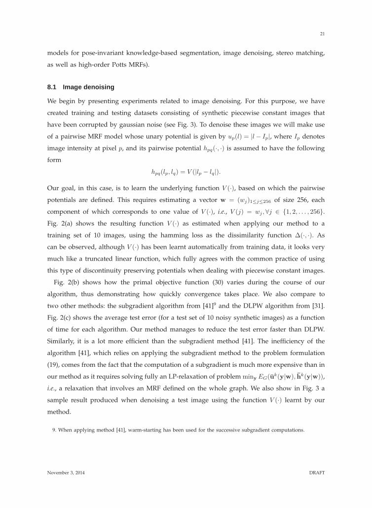
8.1 Image denoising
We begin by presenting experiments related to image denoising. For this purpose, we have
created training and testing datasets consisting of synthetic piecewise constant images that
have been corrupted by gaussian noise (see Fig. 3). To denoise these images we will make use
of a pairwise MRF model whose unary potential is given by up(l) = |l− Ip|, where Ip denotes
image intensity at pixel p, and its pairwise potential hpq(·, ·) is assumed to have the following
form
hpq(lp, lq) = V (|lp − lq|).
Our goal, in this case, is to learn the underlying function V (·), based on which the pairwise
potentials are defined. This requires estimating a vector w = (wj)1≤j≤256 of size 256, each
component of which corresponds to one value of V (·), i.e., V (j) = wj , ∀j ∈ {1, 2, . . . , 256}.
Fig. 2(a) shows the resulting function V (·) as estimated when applying our method to a
training set of 10 images, using the hamming loss as the dissimilarity function ∆(·, ·). As
can be observed, although V (·) has been learnt automatically from training data, it looks very
much like a truncated linear function, which fully agrees with the common practice of using
this type of discontinuity preserving potentials when dealing with piecewise constant images.
Fig. 2(b) shows how the primal objective function (30) varies during the course of our
algorithm, thus demonstrating how quickly convergence takes place. We also compare to
two other methods: the subgradient algorithm from [41]9 and the DLPW algorithm from [31].
Fig. 2(c) shows the average test error (for a test set of 10 noisy synthetic images) as a function
of time for each algorithm. Our method manages to reduce the test error faster than DLPW.
Similarly, it is a lot more efficient than the subgradient method [41]. The inefficiency of the
algorithm [41], which relies on applying the subgradient method to the problem formulation
(19), comes from the fact that the computation of a subgradient is much more expensive than in
our method as it requires solving fully an LP-relaxation of problem miny EG(uk(y|w), hk(y|w)),
i.e., a relaxation that involves an MRF defined on the whole graph. We also show in Fig. 3 a
sample result produced when denoising a test image using the function V (·) learnt by our
method.
9. When applying method [41], warm-starting has been used for the successive subgradient computations.
November 3, 2014 DRAFT
22
0 100 2000
10
20
30
intensity difference
pairwise potential
(a)
0 5 10 15 200
2
4
6x 10⁴
time (secs)
primal objective function
(b)
0 20 40 600
2
4
6
time (secs)
avg
test
err
or
subgradientDLPWour method
(c)
Fig. 2: (a) Learnt pairwise potential V (·), (b) primal objective (30), (c) and average test error as a function
of time for the image denoising problem.
(a) Energy: 6.29× 10⁴ (b) Energy: 8.42× 10⁴ (c) Energy: 5.71× 10⁴ (d) Energy: 6.08× 10⁴
Fig. 3: (a) Noisy test image (b) Denoised image when using a function V (·) estimated during the course
of the learning algorithm (c) Denoised result when using the final V (·) (d) Ground truth image. We also
show below each image the corresponding MRF energy computed using the final estimated V (·).
8.2 Stereo matching
We next test our method on stereo matching, which is a task that requires estimating a per-
pixel disparity map between two images of a stereoscopic pair. For this purpose, we will
use a pairwise MRF with unary potentials given by up(l) = |Ileftp − Irightp−l |, where l represents
discretized disparity, and I left, Iright denote the left and right images, respectively. A very
commonly used pairwise potential in this case is a gradient-modulated Potts model of the
following form:
hpq(lp, lq) = f(|∇I leftp |)[lp 6= lq], (64)
where p, q are neighboring pixels and∇I leftp = I leftp −Ileftq represents the gradient of the left image
at p. Our goal is to automatically learn the function f(·) that is used in the above formula (64)
for assigning a discontinuity penalty based on the magnitude of the image gradient. Function
f(·) can take 256 different values assuming integer intensities and so the positive vector w
that we need to estimate will be of size 256 with wi = f(i). Furthermore, we also impose the
restriction that vector w should belong to the set W = {w ≥ 0|wi ≥ wi+1}, thus reflecting
the a priori knowledge that f(·) should be a decreasing function. To accommodate this into
November 3, 2014 DRAFT
23
0 100 200 3000
5
10
15
20
gradient
function f
(a)
0 10 20 301.5
2
2.5
3x 10⁶
time (secs)
obje
ctiv
e fu
nctio
n
decomp. Gsingle
decomp. Grow−col
(b)
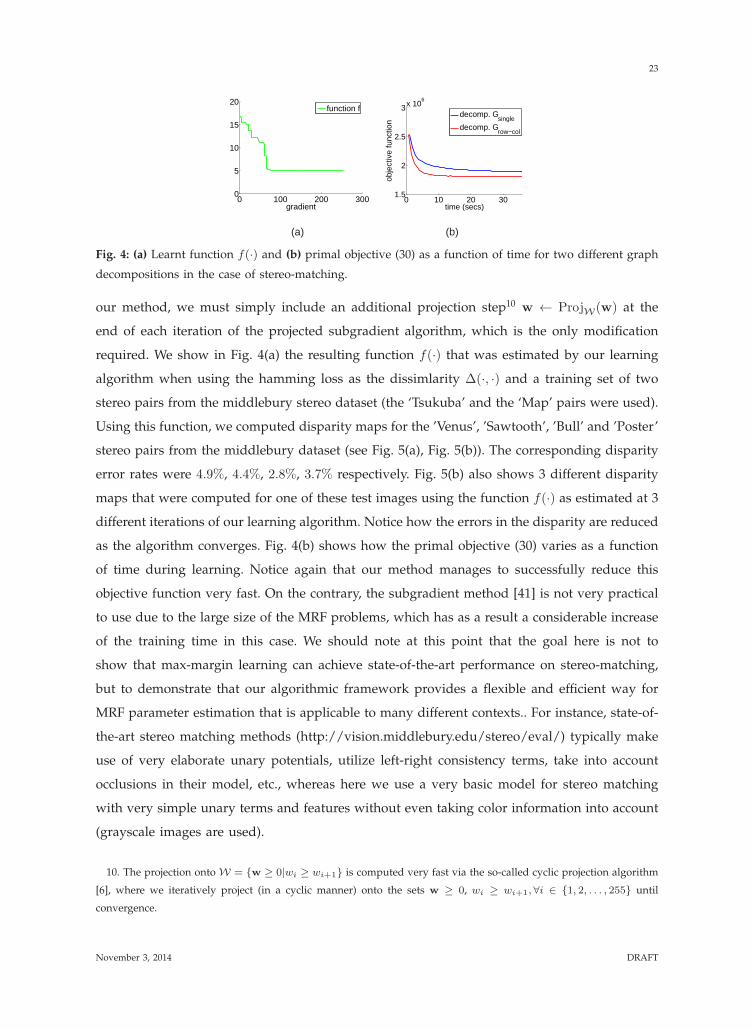
Fig. 4: (a) Learnt function f(·) and (b) primal objective (30) as a function of time for two different graph
decompositions in the case of stereo-matching.
our method, we must simply include an additional projection step10 w ← ProjW(w) at the
end of each iteration of the projected subgradient algorithm, which is the only modification
required. We show in Fig. 4(a) the resulting function f(·) that was estimated by our learning
algorithm when using the hamming loss as the dissimlarity ∆(·, ·) and a training set of two
stereo pairs from the middlebury stereo dataset (the ‘Tsukuba’ and the ‘Map’ pairs were used).
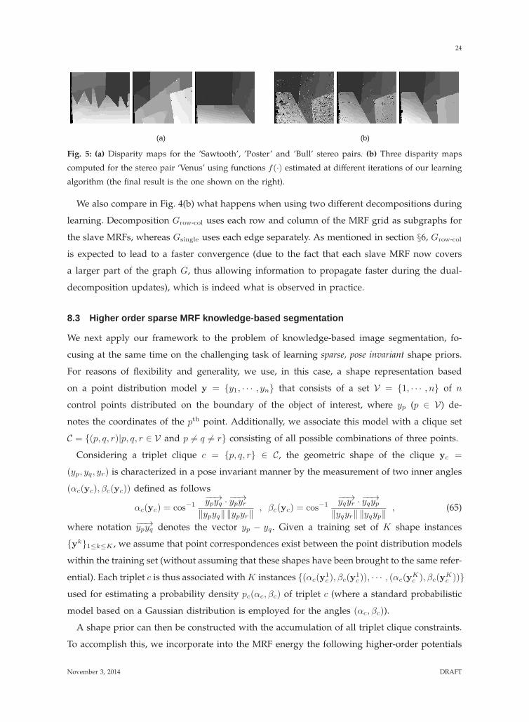
Using this function, we computed disparity maps for the ’Venus’, ’Sawtooth’, ’Bull’ and ’Poster’
stereo pairs from the middlebury dataset (see Fig. 5(a), Fig. 5(b)). The corresponding disparity
error rates were 4.9%, 4.4%, 2.8%, 3.7% respectively. Fig. 5(b) also shows 3 different disparity
maps that were computed for one of these test images using the function f(·) as estimated at 3
different iterations of our learning algorithm. Notice how the errors in the disparity are reduced
as the algorithm converges. Fig. 4(b) shows how the primal objective (30) varies as a function
of time during learning. Notice again that our method manages to successfully reduce this
objective function very fast. On the contrary, the subgradient method [41] is not very practical
to use due to the large size of the MRF problems, which has as a result a considerable increase
of the training time in this case. We should note at this point that the goal here is not to
show that max-margin learning can achieve state-of-the-art performance on stereo-matching,
but to demonstrate that our algorithmic framework provides a flexible and efficient way for
MRF parameter estimation that is applicable to many different contexts.. For instance, state-of-
the-art stereo matching methods (http://vision.middlebury.edu/stereo/eval/) typically make
use of very elaborate unary potentials, utilize left-right consistency terms, take into account
occlusions in their model, etc., whereas here we use a very basic model for stereo matching
with very simple unary terms and features without even taking color information into account
(grayscale images are used).
10. The projection ontoW = {w ≥ 0|wi ≥ wi+1} is computed very fast via the so-called cyclic projection algorithm
[6], where we iteratively project (in a cyclic manner) onto the sets w ≥ 0, wi ≥ wi+1, ∀i ∈ {1, 2, . . . , 255} until
convergence.
November 3, 2014 DRAFT
24
(a) (b)
Fig. 5: (a) Disparity maps for the ’Sawtooth’, ’Poster’ and ’Bull’ stereo pairs. (b) Three disparity maps
computed for the stereo pair ‘Venus’ using functions f(·) estimated at different iterations of our learning
algorithm (the final result is the one shown on the right).
We also compare in Fig. 4(b) what happens when using two different decompositions during
learning. Decomposition Grow-col uses each row and column of the MRF grid as subgraphs for
the slave MRFs, whereas Gsingle uses each edge separately. As mentioned in section §6, Grow-col
is expected to lead to a faster convergence (due to the fact that each slave MRF now covers
a larger part of the graph G, thus allowing information to propagate faster during the dual-
decomposition updates), which is indeed what is observed in practice.
8.3 Higher order sparse MRF knowledge-based segmentation
We next apply our framework to the problem of knowledge-based image segmentation, fo-
cusing at the same time on the challenging task of learning sparse, pose invariant shape priors.
For reasons of flexibility and generality, we use, in this case, a shape representation based
on a point distribution model y = {y1, · · · , yn} that consists of a set V = {1, · · · , n} of n
control points distributed on the boundary of the object of interest, where yp (p ∈ V) de-
notes the coordinates of the pth point. Additionally, we associate this model with a clique set
C = {(p, q, r)|p, q, r ∈ V and p 6= q 6= r} consisting of all possible combinations of three points.
Considering a triplet clique c = {p, q, r} ∈ C, the geometric shape of the clique yc =
(yp, yq, yr) is characterized in a pose invariant manner by the measurement of two inner angles
(αc(yc), βc(yc)) defined as follows
αc(yc) = cos−1−−→ypyq ·
−−→ypyr‖ypyq‖ ‖ypyr‖
, βc(yc) = cos−1−−→yqyr ·
−−→yqyp‖yqyr‖ ‖yqyp‖
, (65)
where notation −−→ypyq denotes the vector yp − yq. Given a training set of K shape instances
{yk}1≤k≤K , we assume that point correspondences exist between the point distribution models
within the training set (without assuming that these shapes have been brought to the same refer-
ential). Each triplet c is thus associated with K instances {(αc(y1c), βc(y
1c)), · · · , (αc(y
Kc ), βc(y
Kc ))}
used for estimating a probability density pc(αc, βc) of triplet c (where a standard probabilistic
model based on a Gaussian distribution is employed for the angles (αc, βc)).
A shape prior can then be constructed with the accumulation of all triplet clique constraints.
To accomplish this, we incorporate into the MRF energy the following higher-order potentials
November 3, 2014 DRAFT
25
0 10 20 30 40 50 60 70 800
500
1000
1500
2000
2500
Time (Second)
Obj
ectiv
e F
unct
ion
(a)
0.75
0.8
0.85
0.9
0.95
Our method ASM
Dic
e C
oeffi
cien
t
(b)
0.55
0.6
0.65
0.7
0.75
0.8
0.85
Our method complete graph Random Walks ASM
Dic
e C
oeff
icie
nt
(c)
Fig. 6: (a) Learning objective function during MRF training with the hand dataset. Boxplots of Dice
coefficients for (b) 2D hand segmentation, and (c) 3D left ventricle segmentation (the Dice coefficient is a
similarity measure between sets X and Y , defined as 2|X∩Y ||X|+|Y |
).
hc(yc)
hc(yc) = −wc log pc(αc(yc), βc(yc)) . (66)
As can be seen, these potentials are parameterized through a vector w = {wc}c∈C containing
one component wc per clique c. Based on the above model, a clique c is essentially ignored if
the corresponding element is close to zero, i.e., if it holds wc ≈ 0. Therefore, the use of w allows
us to reduce the otherwise excessive number of higher order cliques, thus also reducing the
computational cost of inference. Furthermore, given that the significance of the different triplets
towards capturing the observed deformations of the training set is not the same, the role of the
introduced vector w is to also weigh the contribution of those triplets that are retained in the
model. Note that such a shape prior inherits pose invariance so that neither training samples
nor testing shape needs to be aligned in a common coordinates frame. Moreover, it can capture
shape variations even with a small number of training examples.
When applying our max-margin learning method to this problem, we opt to make use of
a sparsity inducing l1-norm regularizer, i.e., R(w) = ||w||1. Such a choice serves the above
purpose of compressing the size of the graph by eliminating as many redundant cliques as
possible (through setting their corresponding weights to zero), thus producing a compact and
efficient representation.
One important issue that the learning needs to address, in this case, relates to the pose-
invariant properties of the learnt shape representation. In other words, it should be able to
account for the fact that if yk is a ground truth shape, then, any transformed shape instance
T (yk), where T (·) represents a similarity transformation, is an equally good solution and
should not be penalized during training. To accomplish that by our method, we make use
of a dissimilarity function ∆(y,y′) that satisfies the following conditions, which ensure that
November 3, 2014 DRAFT
26
(a) Red contours: our results. Blue contours: ASM. Yellow contours: initialization.
(b) Our results on video images with cluttered background.
Fig. 7: 2D hand segmentation results.
pose invariance is indeed taken into account during the training process
(∀y), ∆(T (y),y) = 0 . (67)
The specific function that we use for this purpose decomposes into high-order terms as follows
∆(y,y′) =∑
c∈C δc(yc,y′c), where
δc(yc,y′c) =
0 if the triplets of points yc and y′
c connect by a similarity transform
1 otherwise .
(68)
The aforementioned L1 sparse higher-order shape model is used in conjunction with knowledge-
based segmentation. In this context, following [58] we consider on top of the above third-
order cliques, pair-wise cliques delineating the object boundaries in 2D, or third-order cliques
corresponding to the object surface. The use of generalized Stokes theorem from differential
geometry allows to convert regional integrals to surface ones and therefore combine edge-based
terms with regional ones [57] (thus integrating both edge information and regional statistics
towards seeking the separation in terms of intensity statistical means between the object and
the background). During training, a decomposition that assigns a single clique per slave has
been used, in which case enumeration is applied for solving the resulting slave problems.
Our learning method was evaluated in this context using two different examples, a 2D hand
data-set and a 3D medical imaging example (CT segmentation of the Left Ventricle). The 2D
hand dataset contains 40 right hand examples (20 used for training and 20 used for testing),
showing different poses (i.e., translations, rotations, and scales) and also movements between
the fingers. Manual segmentations on the database are available and used as ground truth, while
November 3, 2014 DRAFT
27
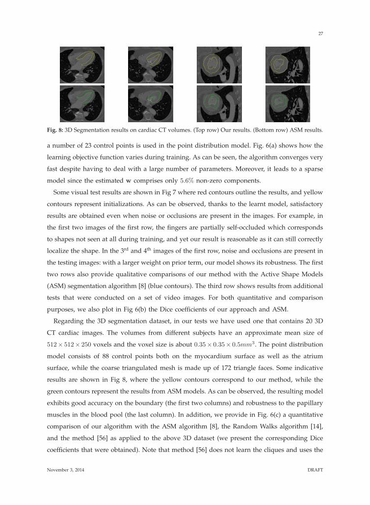
Fig. 8: 3D Segmentation results on cardiac CT volumes. (Top row) Our results. (Bottom row) ASM results.
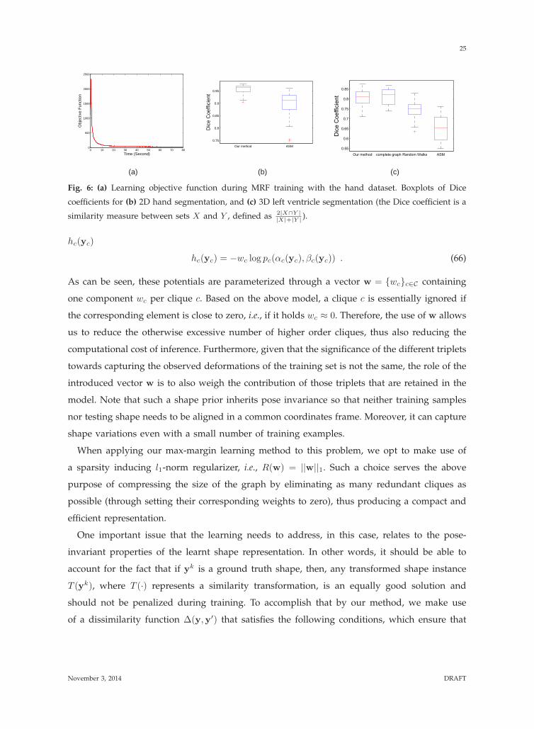
a number of 23 control points is used in the point distribution model. Fig. 6(a) shows how the
learning objective function varies during training. As can be seen, the algorithm converges very
fast despite having to deal with a large number of parameters. Moreover, it leads to a sparse
model since the estimated w comprises only 5.6% non-zero components.
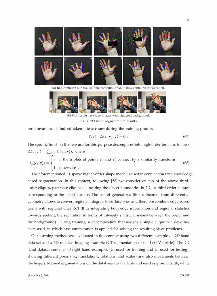
Some visual test results are shown in Fig 7 where red contours outline the results, and yellow
contours represent initializations. As can be observed, thanks to the learnt model, satisfactory
results are obtained even when noise or occlusions are present in the images. For example, in
the first two images of the first row, the fingers are partially self-occluded which corresponds
to shapes not seen at all during training, and yet our result is reasonable as it can still correctly
localize the shape. In the 3rd and 4th images of the first row, noise and occlusions are present in
the testing images: with a larger weight on prior term, our model shows its robustness. The first
two rows also provide qualitative comparisons of our method with the Active Shape Models
(ASM) segmentation algorithm [8] (blue contours). The third row shows results from additional
tests that were conducted on a set of video images. For both quantitative and comparison
purposes, we also plot in Fig 6(b) the Dice coefficients of our approach and ASM.
Regarding the 3D segmentation dataset, in our tests we have used one that contains 20 3D
CT cardiac images. The volumes from different subjects have an approximate mean size of
512× 512× 250 voxels and the voxel size is about 0.35× 0.35× 0.5mm3. The point distribution
model consists of 88 control points both on the myocardium surface as well as the atrium
surface, while the coarse triangulated mesh is made up of 172 triangle faces. Some indicative
results are shown in Fig 8, where the yellow contours correspond to our method, while the
green contours represent the results from ASM models. As can be observed, the resulting model
exhibits good accuracy on the boundary (the first two columns) and robustness to the papillary
muscles in the blood pool (the last column). In addition, we provide in Fig. 6(c) a quantitative
comparison of our algorithm with the ASM algorithm [8], the Random Walks algorithm [14],
and the method [56] as applied to the above 3D dataset (we present the corresponding Dice
coefficients that were obtained). Note that method [56] does not learn the cliques and uses the
November 3, 2014 DRAFT
28
complete graph (it is thus very computationally expensive taking more than 1 hour for one
volume segmentation). On the contrary, we use a very sparse graph since the estimated w
by our method contains only 0.9% non-zero components (the computation time in this case is
about 3 minutes).
8.4 High-order Potts model
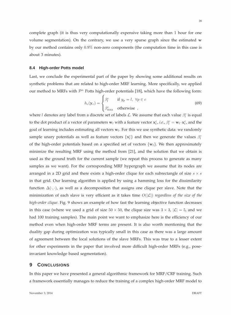
Last, we conclude the experimental part of the paper by showing some additional results on
synthetic problems that are related to high-order MRF learning. More specifically, we applied
our method to MRFs with Pn Potts high-order potentials [18], which have the following form:
hc(yc) =
βcl if yp = l, ∀p ∈ c
βcmax otherwise ,
(69)
where l denotes any label from a discrete set of labels L. We assume that each value βcl is equal
to the dot product of a vector of parameters wl with a feature vector xcl , i.e., βc
l = wl ·xcl , and the
goal of learning includes estimating all vectors wl. For this we use synthetic data: we randomly
sample unary potentials as well as feature vectors {xcl } and then we generate the values βc
l
of the high-order potentials based on a specified set of vectors {wl}. We then approximately
minimize the resulting MRF using the method from [21], and the solution that we obtain is
used as the ground truth for the current sample (we repeat this process to generate as many
samples as we want). For the corresponding MRF hypergraph we assume that its nodes are
arranged in a 2D grid and there exists a high-order clique for each subrectangle of size s × s
in that grid. Our learning algorithm is applied by using a hamming loss for the dissimilarity
function ∆(·, ·), as well as a decomposition that assigns one clique per slave. Note that the
minimization of each slave is very efficient as it takes time O(|L|) regardless of the size of the
high-order clique. Fig. 9 shows an example of how fast the learning objective function decreases
in this case (where we used a grid of size 50 × 50, the clique size was 3 × 3, |L| = 5, and we
had 100 training samples). The main point we want to emphasize here is the efficiency of our
method even when high-order MRF terms are present. It is also worth mentioning that the
duality gap during optimization was typically small in this case as there was a large amount
of agreement between the local solutions of the slave MRFs. This was true to a lesser extent
for other experiments in the paper that involved more difficult high-order MRFs (e.g., pose-
invariant knowledge based segmentation).
9 CONCLUSIONS
In this paper we have presented a general algorithmic framework for MRF/CRF training. Such
a framework essentially manages to reduce the training of a complex high-order MRF model to
November 3, 2014 DRAFT
29
0 20 40 600
2
4
6x 10⁴
time (secs)
obje
ctiv
e fu
nctio
n
Fig. 9: Primal objective function during training of high-order Potts MRFs.
the parallel training of a set of simple slave submodels. We have demonstrated that the derived
learning scheme is sufficiently efficient and flexible (e.g., it can be applied to both pairwise and
high-order models, it requires no submodularity assumptions, and it is easily adapted to the
structure of a given class of MRFs). Moreover, it relies on solid mathematical principles and
enjoys good theoretical properties. Due to all of the above, and given that learning problems
are becoming increasingly important and challenging for a great variety of applications these
days, we believe that our method can find use in a broad class of image analysis and computer
vision tasks. It is also worth noting that this framework can be extended to handle the task of
parameter estimation for latent CRF models [20], in which case a subset of variables remain
unknown (i.e., hidden) during both training and test time. Although not thoroughly discussed
in the present work, these, too, comprise a very important class of models in computer vision,
with an increasingly large number of applications [10], [54].
REFERENCES
[1] K. Alahari, C. Russell, and P. Torr. Efficient piecewise learning for conditional random fields. In CVPR, 2010.
[2] D. Anguelov, B. Taskar, V. Chatalbashev, D. Koller, D. Gupta, G. Heitz, and A. Ng. Discriminative learning of
markov random fields for segmentation of 3d scan data. In CVPR, 2005.
[3] D. Bertsekas. Nonlinear Programming. 1999.
[4] J. Besag. Efficiency of pseudolikelihood estimation for simple Gaussian fields. Biometrika, 64(3):616–618, Dec. 1977.
[5] A. Blake, P. Kohli, and C. Rother. Advances in Markov random fields for vision and image processing. MIT Press, 2011.
[6] Y. A. Censor and S. A. Zenios. Parallel Optimization: Theory, Algorithms and Applications. Oxford University Press.
[7] C. Chekuri, S. Khanna, J. Naor, and L. Zosin. Approximation algorithms for the metric labeling problem via a
new linear programming formulation. In SODA, 2001.
[8] T. F. Cootes, C. J. Taylor, D. H. Cooper, and J. Graham. Active shape models: their training and application.
Comput. Vis. Image Underst., 61(1):38–59, Jan. 1995.
[9] J. Domke. Learning graphical model parameters with approximate marginal inference. in IEEE TPAMI, 2013.
[10] P. Felzenszwalb, R. Girshick, D. McAllester, and D. Ramanan. Object detection with discriminatively trained
part-based models. IEEE TPAMI, 2009.
[11] T. Finley and T. Joachims. Training structural svms when exact inference is intractable. In ICML, 2008.
[12] V. Franc and B. Savchynskyy. Discriminative learning of max-sum classifiers. JMLR, 2008.
[13] S. Gould. Max-margin learning for lower linear envelope potentials in binary mrfs. In ICML, 2011.
[14] L. Grady. Random walks for image segmentation. IEEE Trans. Pattern Anal. Mach. Intell., 2006.
[15] T. Hazan and R. Urtasun. A primal-dual message-passing algorithm for approximated large scale structured
prediction. In NIPS, pages 838–846, 2010.
[16] G. E. Hinton. Training products of experts by minimizing contrastive divergence. Neural Computation, 2002.
November 3, 2014 DRAFT
30
[17] J. H. Kappes, B. Andres, F. A. Hamprecht, C. Schnorr, S. Nowozin, D. Batra, S. Kim, B. X. Kausler, J. Lellmann,
N. Komodakis, and C. Rother. A comparative study of modern inference techniques for discrete energy
minimization problem. In CVPR, 2013.
[18] P. Kohli, P. Kumar, and P. Torr. P3 and beyond: Solving energies with higher order cliques. In CVPR, 2007.
[19] N. Komodakis. Efficient training for pairwise or higher order CRFs via dual decomposition. In CVPR, 2011.
[20] N. Komodakis. Learning to cluster using high order graphical models with latent variables. In ICCV, 2011.
[21] N. Komodakis and N. Paragios. Beyond pairwise energies: Efficient optimization for higher-order MRFs. In
CVPR, 2009.
[22] N. Komodakis, N. Paragios, and G. Tziritas. MRF optimization via dual decomposition: Message-passing revisited.
In ICCV, 2007.
[23] N. Komodakis, N. Paragios, and G. Tziritas. MRF energy minimization and beyond via dual decomposition.
PAMI, 2010.
[24] P. Kumar, B. Packer, and D. Koller. Modeling latent variable uncertainty for loss-based learning. In ICML, 2012.
[25] S. Kumar, J. August, and M. Hebert. Exploiting inference for approximate parameter learning in discriminative
fields: An empirical study. In EMMCVPR, 2005.
[26] S. Kumar and M. Hebert. Discriminative random fields. International Journal of Computer Vision, 2006.
[27] J. D. Lafferty, A. McCallum, and F. C. N. Pereira. Conditional random fields: Probabilistic models for segmenting
and labeling sequence data. In ICML, 2001.
[28] S. Z. Li. Markov Random Field Modeling in Image Analysis. Springer, 2009.
[29] Y. Li and D. P. Huttenlocher. Learning for stereo vision using the structured support vector machine. In CVPR,
2008.
[30] D. A. McAllester, T. Hazan, and J. Keshet. Direct loss minimization for structured prediction. In NIPS, 2010.
[31] O. Meshi, D. Sontag, T. Jaakkola, and A. Globerson. Learning efficiently with approximate inference via dual
losses. In ICML, 2010.
[32] K. Miller, M. P. Kumar, B. Packer, D. Goodman, and D. Koller. Max-margin min-entropy models. 2012.
[33] D. Munoz, J. A. Bagnell, and M. Hebert. Stacked hierarchical labeling. In ECCV, 2010.
[34] D. Munoz, J. A. D. Bagnell, N. Vandapel, and M. Hebert. Contextual classification with functional max-margin
markov networks. In CVPR, 2009.
[35] K. Murphy, Y. Weiss, and M. Jordan. Loopy-belief propagation for approximate inference: An empirical study. In
UAI, 1999.
[36] A. Nedic and D. P. Bertsekas. Incremental subgradient methods for nondifferentiable optimization. SIAM J. on
Optimization, 2001.
[37] S. Nowozin, C. Rother, S. Bagon, T. Sharp, B. Yao, and P. Kohli. Decision tree fields. In ICCV, 2011.
[38] G. Papandreou and A. Yuille. Perturb-and-map random fields: Using discrete optimization to learn and sample
from energy models. In ICCV, 2011.
[39] K. Park and S. Gould. On learning higher-order consistency potentials for multi-class pixel labeling. In ECCV,
2012.
[40] P. Pletscher and P. Kohli. Learning low-order models for enforcing high-order statistics. In AISTATS, 2012.
[41] N. Ratliff, J. A. D. Bagnell, and M. Zinkevich. (online) subgradient methods for structured prediction. In AISTATS,
2007.
[42] K. G. G. Samuel and M. F. Tappen. Learning optimized map estimates in continuously-valued mrf models. In
CVPR, 2009.
[43] D. Scharstein and C. Pal. Learning conditional random fields for stereo. In CVPR, 2007.
[44] M. Schlesinger and V. Giginyak. Solution to structural recognition (MAX,+)-problems by their equivalent
transformations. Control Systems and Computers, 2007.
[45] A. G. Schwing, T. Hazan, M. Pollefeys, and R. Urtasun. Efficient structured prediction with latent variables for
general graphical models. In ICML, 2012.
[46] S. Shalev-Shwartz, Y. Singer, and N. Srebro. Pegasos: Primal estimated sub-gradient solver for svm. In ICML,
November 3, 2014 DRAFT
31
2007.
[47] D. Sontag, O. Meshi, T. Jaakkola, and A. Globerson. More data means less inference: A pseudo-max approach to
structured learning. In NIPS, pages 2181–2189, 2010.
[48] R. Szeliski, R. Zabih, D. Scharstein, O. Veksler, V. Kolmogorov, A. Agarwala, M. Tappen, and C. Rother. A
comparative study of energy minimization methods for markov random fields with smoothness-based priors.
IEEE Trans. Pattern Anal. Mach. Intell., 30(6):1068–1080, June 2008.
[49] M. Szummer, P. Kohli, and D. Hoiem. Learning CRFs using graph cuts. In ECCV, 2008.
[50] M. F. Tappen, K. G. G. Samuel, C. V. Dean, and D. M. Lyle. The logistic random field - a convenient graphical
model for learning parameters for mrf-based labeling. In CVPR, 2008.
[51] D. Tarlow, R. Adams, and R. Zemel. Randomized optimum models for structured prediction. In AISTATS, 2012.
[52] D. Tarlow and R. S. Zemel. Structured output learning with high order loss functions. In AISTATS, 2012.
[53] B. Taskar, C. Guestrin, and D. Koller. Max-margin markov networks. In NIPS, 2004.
[54] H. Wang, S. Gould, and D. Koller. Discriminative learning with latent variables for cluttered indoor scene
understanding. In ECCV, 2010.
[55] T. Werner. A linear programming approach to max-sum problem: A review. PAMI, 2007.
[56] B. Xiang, C. Wang, J. Deux, A. Rahmouni, and N. Paragios. 3d cardiac segmentation with pose-invariant higher-
order mrfs. In ISBI 2012, pages 1425–1428. IEEE, 2012.
[57] B. Xiang, C. Wang, J.-F. Deux, A. Rahmouni, and N. Paragios. Tagged cardiac mr image segmentation using
boundary & regional-support and graph-based deformable priors. In ISBI, pages 1706–1711, 2011.
[58] B. Xiang, C. Wang, J.-F. Deux, A. Rahmouni, and N. Paragios. 3d cardiac segmentation with pose-invariant
higher-order mrfs. In ISBI, pages 1425–1428, 2012.
[59] P. Yadollahpour, D. Batra, and G. Shakhnarovich. DivMCuts: Faster Training of Structural SVMs with Diverse
M-Best Cutting-Planes. In AISTATS, 2013.
[60] C.-N. J. Yu and T. Joachims. Learning structural SVMs with latent variables. In ICML, 2009.
Nikos Komodakis is associate professor at Universite Paris-Est, Ecole des Ponts ParisTech and
research scientist at the UMR Laboratoire d’informatique Gaspard-Monge, CNRS. He is also an
affiliated adjunct professor at Ecole Normale Suprieure de Cachan. He currently serves as an
editorial board member for the International Journal of Computer Vision and the CVIU journal.
His research interests are in the areas of computer vision, image processing, machine learning
and medical imaging, and has published numerous papers in the most prestiguous journals and
conferences from the above domains.
Bo Xiang received her PhD degree in Applied Mathematics from Ecole Centrale de Paris. Her
research interests include computer vision, medical image analysis and machine learning. Her
PhD thesis focuses on graphic models towards segmentation. Before her PhD study, she received
the B.Sc. from Fudan University, and M.Eng. from Graduate University of Chinese Academy of
Sciences in China, in 2006 and 2009 respectively.
November 3, 2014 DRAFT

32
Nikos Paragios is professor of applied mathematics at Ecole Centrale de Paris and scientific
leader of the Galen team at INRIA, Saclay Ile-de-France Unit. He has published more than 200
papers in the most prestigious journals and conferences of computer vision, biomedical imaging
and machine learning. He currently serves as the Editor in Chief of the Computer Vision and Image
Understanding Journal while he has also served/serves as a member of the editorial boards for
numerous journals of his scientific fields.
November 3, 2014 DRAFT
Related Documents