1 · 2 Slat designed to retract to form main airfoil leading edge. 42 3 Flow about a circular cylinder with circulation r c. 43 ... 6 Pole airfoil geometry and velocity ...

llteo""'>duced by

NATIONAL TECHNICAL INFORMATION SERVICE

Spn ngf,.,k:l, Va. 22151

/ MCDONNELL DOCJGL~

(,7

• UNCLA SSI FIED • ~curi l y C I:.J n ,.ific ,.tlll n

(Sttct6lt'!' clo ••lllcelltM ol 1111•. twdy1 ol •befr•c l e :"td lud~ :x ln 1IVInoteUo.n tu v e t be e nt•r• d ' " "'~~ lite o wutU r•pnrt I• r-l• ••llled)

t ORIGINATING A Ct iVITY (Corpotafe • u :lttA) ~. fH::.POHl S E CURITY CL4~ ~U,...IC 4TION

DOUGL/\S AIRCRAFT COHPAHY 't-1cDONNELL DOUGLAS CORPO ATION

UNCJ..J\ S~ IF IED 2b, CO ROU P

3855 LAKEWOOD BLVD. _H>::.>N:.::IG~BE;:;· A~C:;,;H,;.;.i...,..;:C~A.;;;,L:;,;IF;..;· O;.;;R,;;.,N...:::I;;.:A_...;9;..;0:;..;;8;...;;0...:::l~L---------------i ) . I"< EPO RT TITLE

THEORETICAL STUDIES ON THE AERODYNA't-1ICS OF Sh~T-AIRFOIL COrffiiNATIONS

• . DESCRIPTIVE NOTIES (Typo of r.,_: -d lfld-l•o ••••J Scientific Fina ~

• · AU THOR lSI (Fire I ,..,.,., alddlo hdtlal, IAel:" .-=:-=)-:-----------------------------·---1

ROBERT H LIEBECK

• . ~' E PO" T DATE

28 Hay 1971 ... CONTPACT OR CORAHT NO .... ORIGOI N ATOII<'I RE~ORT NUWa&RCSI

6, PROJIEC T NO.

F44620-70-C-Ol08 9781-02 HDC J5195

c.

d.

61102F

681307

H . O TUi.R fti!PORT NOISI ( Any otlww ...-beta .,._, _ , bo oee/IJno d Uti• ,.,.,.)

10 . DISTRIBUTION ITAT ILWE NT

Approved for public r e l ease; distr i bution unlimi t ed .

11 . $UP PL EWENTAR\' HOTEl

TECH, OTHER

U . A BSTR ACT

1&. S II'ONIOAING MILITAA\' ACTIVIT\'

AF Office of Scientific Res ear ch (NAM) 1400 \-lilson Boulevard Arlin!!ton Vir!!inia 22209

'Ph"tS ;..·eport des cribes the results of a theore tical study on the analysis and de si~n , of leading e dge slat plus main air foil combina tion;;: ~1:'ginall: it ~.,as planned ; to approach this problem~ ~sing thre •bas ic me thods: ~ epresentat ion of the slat by a point vortex, .U.. .Represeutation of the slat by a set of thin airfoil theory singularity distributions. nd III. exact solution of the complete t\W I element airfoil problem using conforma l mapping methods. After developing the basic analytical wor!< for me thod III, it became .;~ p par nt that the r emaining analysis an d computer programming r equ ired for even a rud im nt a y eva luat ion of this approa ch w ld exceed the total time available for the entire s :: udy . Therefore, it Has decided to concentrate on the ~evelopment of Methods I and II. An ~ n-line " ~omputer ~ ' c: p.:-ogramJwe'e ' prepared for tfte solution and evaluation ' o Me thod I, J ;rhe main airfoil 1~ chos e·n from an infinite set of airfoils whos e mapping functions to the unit circle are analytically de f ine d. ~ (The cla ssical Joukows ki a ir f oils are members of this set . ) The vortex s t r . ng t ~ and position with respect to the main airfoil i~ then prescribed anr·· t ' 1~ progr~m calculates and displa ys the velocit y ! distribution on the air foil wi t · , a d without he vortex present. This program has ' been applie d to the stully and deve lopment o f some basic slat design guide lines l which are presente d. The problem of designing ' l ea ding edge slat wftieft provida8 ; a spe cified velocity; modulation on the nos e r eg ion of a m;:tin airfo il hes lil ~an- ,, .. !. ! studied using the ~r-'Hlcl ~thod {1. A computer progro m has been pr e pare d ! which for a given slat thickness distribu~~ designs a slat cam'!.>e r line t ha t providee a specified v~locity modula tion ;;~ e nose r egion of an e llip3e. Sample results arc include d for a limite d set of t est cases.

UNCLASSIFIED Security Caaaslfocal inn

— i i II wii ■■ mi\wm*mamm ■ wmmm w m w*"'"-*"* PB» i ■ i n ■

,*t uNcij\s.sirn;i) f>«cuMty Cloamdrvtlon

NCV «OMOt LINK A

nokt

LIMK C

nod NOLC

AERODYNAMICS

AIRFOIL

LEADING-EDGE SLAT

MULTI-ELEMENT AIRFOIL

UNCLASSIFIED Sacvrlty Cli>«*lflcauo«

MMIIjllBaatflliaiMly1 ■----—~-^*

' » ■ ^m^^9^**~~*

THEORETICAL STUDIES ON THE AERODYNAMICS OF

SLAT-AIRFOIL COMBINATIONS

by

Robert H. Llebeck

Report No. MDC J5195 28 May 1971

FINAL REPORT

This work was performed under

Contract No. F44620-70-C-0108 for the

Air Force Office of Scientific Research

Washington, D. C.

't**^'"

Hum^Httmammmmmiiaäm^mtait^Ktmmmm —

"• ' ■^^^■^l""1 ■ PI

Copy numbtr Rtport numbtr MDC J5195

THEORETICAL STUDIES ON THE AERODYNAMICS OF

SLAT-AIRFOIL COMBINATIONS

Revision date Revision letter

Issue date 28 May 1971 Contract number

Prepared by Robert H' Liebeck

Approved by:

«üTl. Hess, Chief 44-

. Hess. Chief Basic Research Group for Aerqc(ynaplc

fH U. Dunn Director of Aerodynamics

A. H. Ü. Smith —^^^L

Chief Aerodynamics Engineer Research

This work was performed under

Contract No. F44620-70-C-0108 for the

Air Force Office of Scientific Research

Washington, D. C.

AtCOOJV/Vf I.L OOt/Ot-ÜÜS

i

OOJtMMMTfOW

ffiiir<innilTTiliMtih -n «fUMllMlifl II ' - [ll-lllWrilll i i «fl r

wmmmmmm

MÜC J5195

1.0 ABSTRACT

This report describes the results of a theoretical study on the analysis and

design of leading edge slat plus main airfoil combinations. Originally It

was planned to approach this problem using three basic methods: I. Repre-

sentation of the slat by a point vortex, II. Representation of the slat by

a set of thin airfoil theory singularity distributions, and III. Exact solu-

tion of the complete two element airfoil problem using conformal mapping

methods. After developing the basic analytical work for Method III, It be-

came apparent that the remaining analysis and computer programming required

for even a rudimentary evaluation of this approach would exceed the total

time available for the entire study. Therefore, It was decided to concentrate

on the development of Methods I and II.

An "on-Vine" computer graphics program was prepared for the solution and

evaluation of Method I. The main airfoil Is chosen from an Infinite set of

airfoils whose mapping functions to the unit circle are analytically defined.

(The classical Joukowskl airfoils are members of this set.) The vortex

strength and position with respect to the main airfoil Is then prescribed and

the program calculates and displays the velocity distribution on the airfoil

with and without the vortex present. This program has been applied to the

study and development of some basic slat design guidelines which are pre-

sented In this report.

The problem of designing a leading edge slat which provides a specified velo-

city modulation on the nose region of a main airfoil has been studied using

the approach of Method II. A computer program has been prepared which for

a given slat thickness distribution designs a slat camber line that provides

a specified velocity modulation on the nose region of an ellipse. Sample

results are Included for a limited set of test cases.

— ■ -1 ■

11 in ii in i—

i-—---»™w-»-w--~w~-i^w^r»>i™w^^w»wT~|w»w™»-T^'--r7'

MDC J519S

2,0 TABLE OF CONTENTS

1.0 ABSTRACT

2.0 TABLE OF CONTENTS

3.0 LIST OF FIGURES

4.0 LIST OF SYMBOLS

5.0 INTRODUCTION

6.0 POINT VORTEX MODEL

6.1 General Discussion

6.2 Results and Conclusions

7.0 DISTRIBUTED SINGULARITY MODEL

7.1 General Discussion

7.2 Description of Analysis

7.3 Results and Conclusions

8.0 REFERENCES

Page No.

1

2

3

5

7

12

12

15

22

22

24

37

40

J

A m

i -- ii i MiiillMiMiiriri mi ill'

nw*~F<—^*imm

■*^V>V '■•'«wrw.. rrrrnjum*

MDC J5195

3.0 LIST OF FIGURES

No. Title Page No.

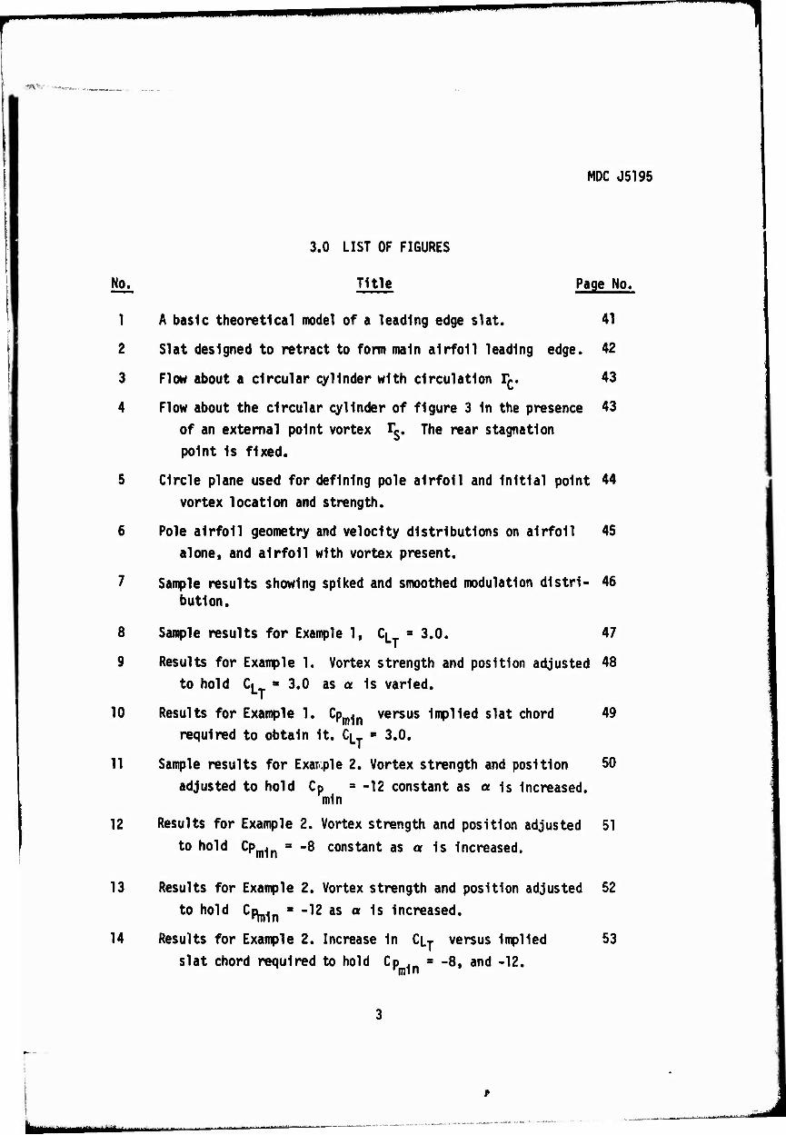
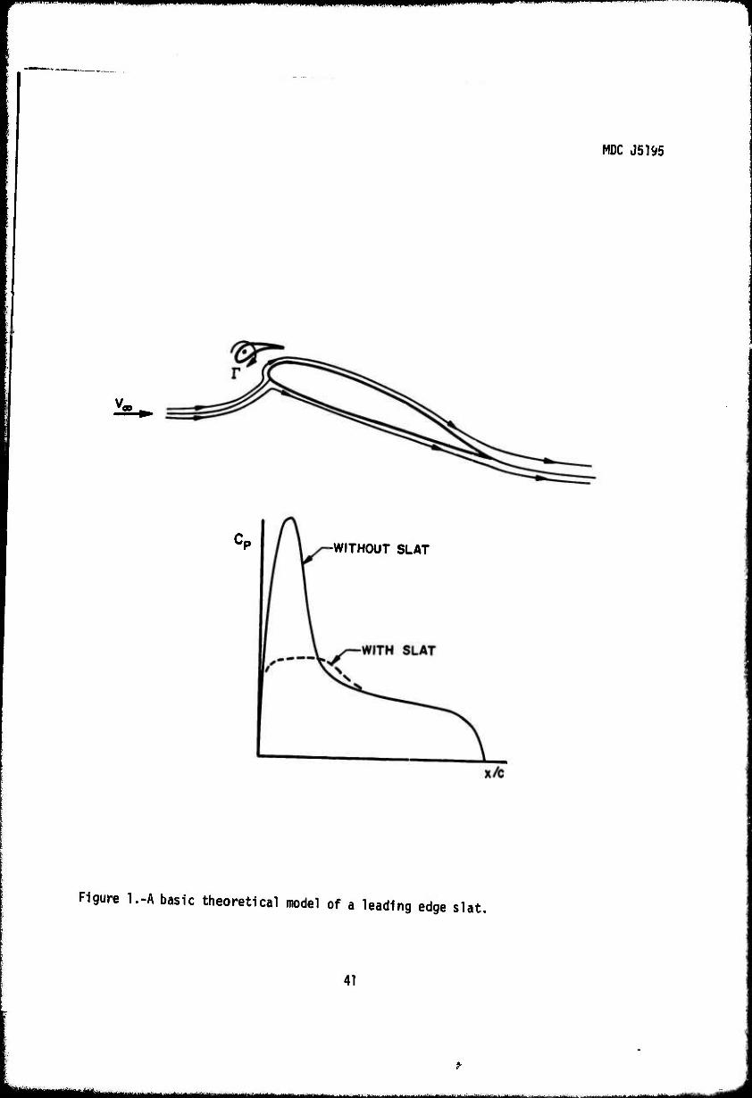
1 A basic theoretical model of a leading edge slat. 41

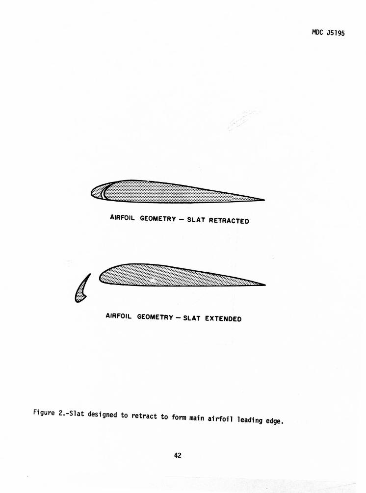
2 Slat designed to retract to form main airfoil leading edge. 42

3 Flow about a circular cylinder with circulation rc. 43

4 Flow about the circular cylinder of figure 3 In the presence 43 of an external point vortex l^. The rear stagnation point Is fixed.

5 Circle plane used for defining pole airfoil and Initial point 44 vortex location and strength.

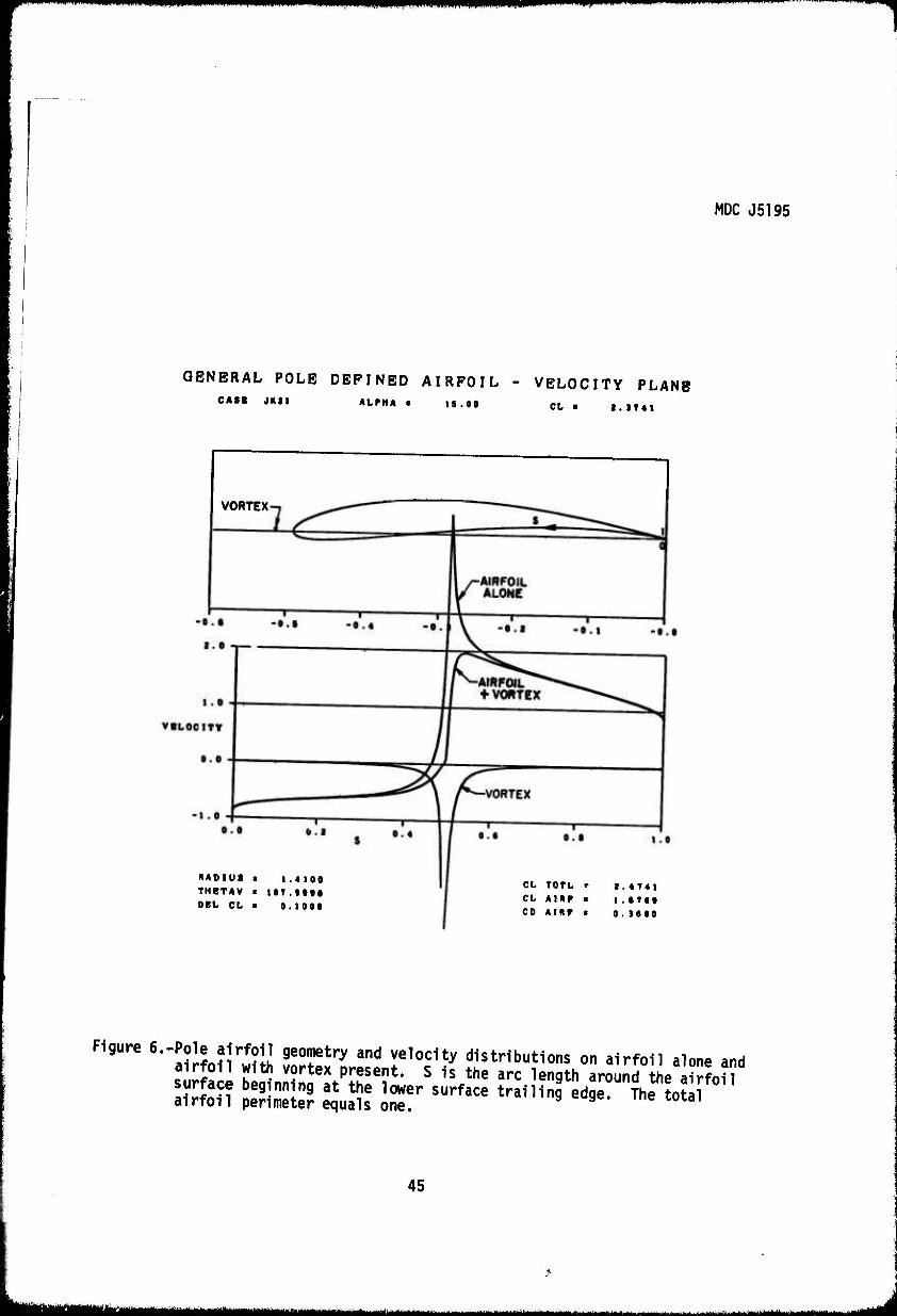
6 Pole airfoil geometry and velocity distributions on airfoil 45 alone, and airfoil with vortex present.

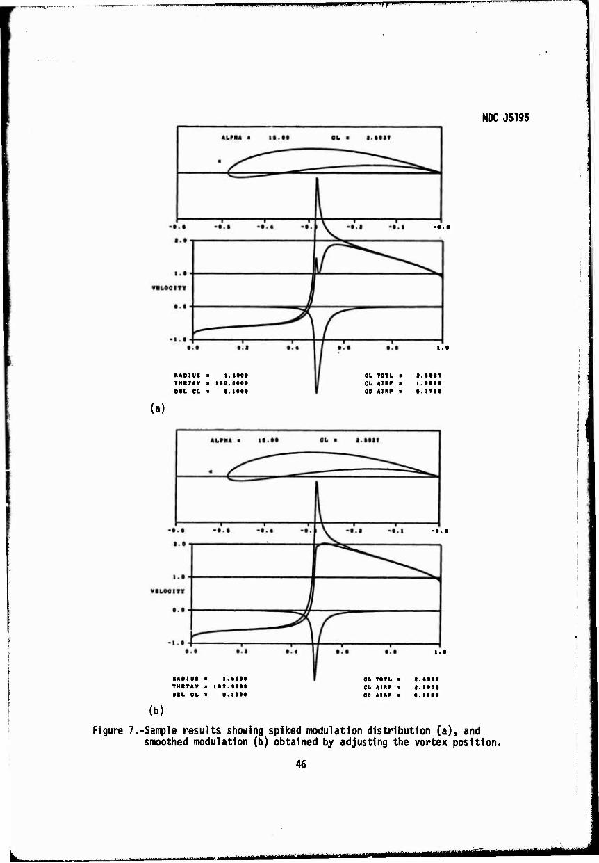
7 Sample results showing spiked and smoothed modulation dlstrl- 46 button.

8 Sample results for Example 1, Ci a 3.0. 47

9 Results for Example 1. Vortex strength and position adjusted 48 to hold C. s 3.0 as a Is varied.

10 Results for Example 1. Cpm1n versus Implied slat chord 49 required to obtain It. CL- S 3.0.

11 Sample results for Example 2. Vortex strength and position SO adjusted to hold Cp s -12 constant as a is Increased.

rain

12 Results for Example 2. Vortex strength and position adjusted 51 to hold Cp^ = -8 constant as a Is Increased.

13 Results for Example 2. Vortex strength and position adjusted 52 to hold CpL..- ■ -12 as a Is Increased.

14 Results for Example 2. Increase In CL-T versus Implied 53 slat chord required to hold Cp . = -8, and -12.

■»"-'"■««»PIDPW»^»^""""«^'"^

MDC J5195

No. Title Page No.

15 Sample results for Example 3. 54

16 Sample results for Example 3. Vortex position fixed at 55

« > 25°. Vortex strength adjusted to obtain proper

modulation as a Is reduced.

17 Results for Example 3. Variation of lift coefficients 06

with a, vortex position set a « 25°, and vortex

strength adjusted to obtain proper modulation at

lower a's.

18 Results for Example 4. Comparison of point vortex with 57

a real slat using the Douglas Neumann potential flow

program.

19 Results for Example 5. Point vortex used to simulate a 58

slotted flap.

20 Domains used In the distributed singularity analysis. 59

21 Geometric mode shapes for uniform onset flow In the 60

S-plane.

22 Ellipse nose pressure modulation: desired modulated pres- 61

sure distribution and that provided by the slats of

figure 23.

23 Slats designed to provide the same modulation on the 62

nose of the 14X thick ellipse.

mm ** ' m—8 1 " '^MiL^äijtMMUuLM^aiii&täimutfmmii M$

^-r-.- ^-~ N m mil ii iiiiiiiiimi. i wm^i^mf^mmiK^m „mmwmitmmmKf» D ■ '" Wfm

H.nn-^TX.' W»w«»*«w* a

MDC J5195

4.0 LIST OF SYMBOLS

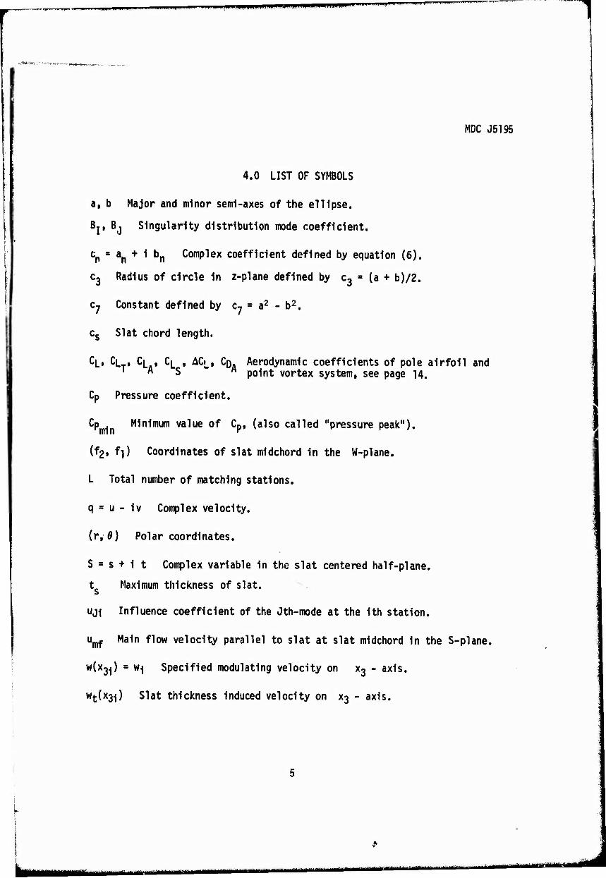
a, b Major and minor semi-axes of the ellipse.

Bj, Bj Singularity distribution mode coefficient.

cn = an + 1 bn Complex coefficient defined by equation (6).

c3 Radius of circle In z-plane defined by c3 = (a + b)/2.

c7 Constant defined by c7 = a2 - b2,

cs Slat chord length.

CL» CLT» CL » CL , ACj_f CQ Aerodynamic coefficients of pole airfoil and 1 A S ' M point vortex system, see page 14.

Cp Pressure coefficient.

■mln Minimum value of Cp, (also called "pressure peak").

(fgi f]) Coordinates of slat mldchord In the W-plane.

L Total number of matching stations,

q = u - 1v Complex velocity.

(r,ö) Polar coordinates.

S = s + 1 t Complex variable In the slat centered half-plane.

t. Maximum thickness of slat, s

uji Influence coefficient of the Jth-mode at the 1th station.

u^ Main flow velocity parallel to slat at slat mldchord in the S-plane.

W(X3J) = w.( Specified modulating velocity on X3 - axis.

Wt(x3i) Slat thickness induced velocity on X3 - axis.

mmmmmm ^uaUkaMMlikia

I'H'II l'HHi HH-IWHIlll.llHIIHHIIl^mrr»^!"»»"1^«! UTTHf 1 l-l-i'-'T-l'l

W = x3 + i y3 Complex varlabla In the half-plane.

z = Xg + 1 y2 Complex variable In the circle-plane.

Z " X| + 1 y. Complex variable In the ellipse-plane.

a Airfoil angle of attack.

o^ Slat chord angle with respect to x3-ax1s In the W-plane

rA Adjusting circulation on circular cylinder.

rc Circulation on circular cylinder.

T- Point vortex circulation.

S| Defined on page 29.

<jb Defined on page 30.

id {= r e Complex variable defined by equation (7).

( ).j Refers to the 1th matching station.

(),,(), Refers to the Ith or Jth mode.

-..,.,.,- ■.. ; ..-^...^ | | ■■- ,.-^^aMim^^^^^^L^^ääMhmiiiiuiaäkt

mmminmimmmmmmm^^ wrwmmimmmmmmm***~mm*w*

MDC J5195

5.0 INTRODUCTION

The designer of high lift systems for modern aircraft Is faced with a severely

over-constrained problem. The satisfaction of cruise configuration geometry together with structural and mechanical requirements quite often results in a high lift system which Is les* than optimum aerodynamical 1y. An additional complication results from the fact that even If the structural and mechanical

requirements were relaxed, the aerodynamic design of high lift systems Is

still quite empirical and heavily reliant on wind tunnel testing. It Is the

purpose of this study to attempt to Increase the knowledge and understanding

of one of the basic components of a high lift system, the leading edge slat.

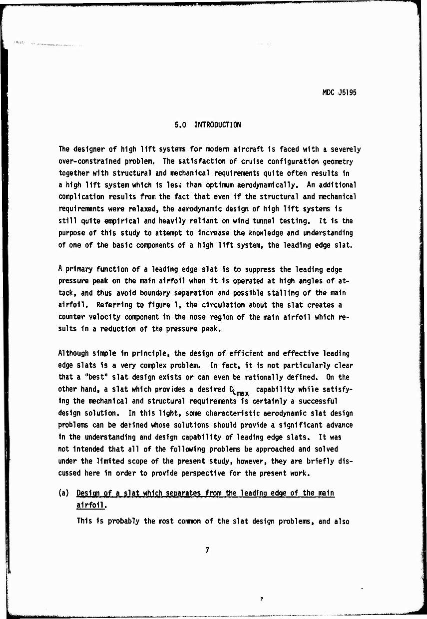
A primary function of a leading edge slat Is to suppress the leading edge pressure peak on the main airfoil when It Is operated at high angles of at-

tack, and thus avoid boundary separation and possible stalling of the main airfoil. Referring to figure 1, the circulation about the slat creates a

counter velocity component In the nose region of the main airfoil which re- sults In a reduction of the pressure peak.

Although simple In principle, the design of efficient and effective leading

edge slats Is a very complex problem. In fact. It Is not particularly clear

that a "best" slat design exists or can even be rationally defined. On the

other hand, a slat which provides a desired CL capability while satisfy-

ing the mechanical and structural requirements Is certainly a successful

design solution. In this light, some characteristic aerodynamic slat design

problems can be defined whose solutions should provide a significant advance

In the understanding and design capability of leading edge slats. It was

not Intended that all of the following problems be approached and solved

under the limited scope of the present study, however, they are briefly dis-

cussed here In order to provide perspective for the present work.

(a) Design of a slat which separates from the leading edge of the main

airfoil.

This Is probably the most common of the slat design problems, and also

'■^ —'■' """ ' "■ "■ ''linn iiiiniiii .■ i) pwpppp^wWWPHWIfHWIflwIiT» mi,-i unWPWWf

MDC J5195

the most difficult from the aerodynamlcist's point of view. Here the

main airfoil geometry Is already specified and the designer Is asked to separate a portion of the leading edge to form a slat as shown In figure 2. The upper surface geometry of the slat Is fixed, and the lower sur-

face of the slat and the slat and the nose of the main airfoil must be

shaped so they will fit together when the slat Is retracted as shown In

figure 2. The resulting slat Is then oriented with respect to the main

airfoil to provide the desired performance.

(b) Design of a slat which provides a specified modulated pressure distri- bution on the nose region of a given main airfoil.

This problem Is less constrained than problem (a) above. The slat geo-

metry and orientation are left completely free and It Is only required that the resulting slat provides the specified pressure modulation dis-

tribution on the nose of the main airfoil. In addition, the flow should not separate on the slat Itself.

(c) Simultaneous design of both the slat and the main airfoil.

It Is obvious that this problem requires at least some generalized con- straints or performance goals to have any solution at all. However a capability In this area could provide solutions to more specific problems such as: "design a two element airfoil system which obtains the maximum

possible lift without separation".

Problems (a), (b), and (c) above are of course not distinct, nor do they

represent In themselves the entire spectrum of leading edge slat design prob-

lems. They do serve to Illustrate the basic forms which such problems take

on, and this suggests the types of analyses which are most suitable In attempt-

ing to obtain design solutions.

There exist several theoretical analysis methods which may be applied to the

leading edge slat design and analysis problems Just described. One of the

most powerful and versatile methods for the analysis of a multi-element

8

i iiB^Mi^^^^^Mi^—iMMiMia—rt—iMui

mmm

^iflrtfU?'^-' .;.*w*wi«».i'.! \. .'.-.■.■ ;

MDC J5195

airfoil system of specified geometry Is the Douglas Neumann potential flow

computer program (reference 1). This program provides exact solutions for

the potential flow field (on and off the bodies) for multi-element airfoil

systems of up to five elements, and therefore Is an extremely valuable tool

for evaluating and predicting the aerodynamic performance of leading edge

slat designs. This type of solution Is called "direct" In that It requires

the airfoil and slat geometry as an Input. It can be used as a design tool

by examining the results for a particular geometry, and then adjusting the geometry and re-running the program until the desired performance Is obtained.

Unfortunately the determination of what geometry adjustments should be made

requires considerable experience and Intuition, and this procedure tends

to be rather costly and time-consuming. However, this approach appears to be the best available for problem (a) above at this time.

An analytic procedure for Iterating with direct solution results has been

developed by Wilkinson In reference 2 for the design of m'iltl-element air-

foil systems. The pressure distributions on the upper surfaces of the air-

foil elements are prescribed, and an Initial geometry Is specified. Wilkinson's Iterative procedure then systematically modifies the camber distributions of

the airfoil elements. The maximum thicknesses, thickness distributions, chord lengths, and gaps between airfoil elements are maintained at all stages as

equal to the respective quantities on the Initial geometry. The advantage of this type of method lies In the fact that If a final solution Is obtained

(I.e. it converges) It Is exact. However, there Is no guarantee that an

arbitrarily Input set of Initial geometries and upper surface pressure dis-

tributions can be Iterated to convergence. This method Is useful for apprcach-

Ing the solution of problem (c) above.

O'Pray in reference 3 has developed a linearized solution for problem (b) which

for a given slat chord, slat orientation, and slat thickness distribution,

shapes the slat camber line to provide the specified pressure modulation dis-

tribution on the nose region of the main airfoil. It appears, in principle,

that this method can be extended to obtain a partial solution to problem (a):

namely, Instead of specifying the slat thickness distribution, the slat upper

surface shape could be specified.

m*

—-"— tmm pnnw unimwiii n m^mmmmi'milt*^*'*^**^"'1 * """" i m IM|I^ II RPIIBI ailWIRIIII I

HOC J5195

In the present work, It was originally decided to study the problem of lead- ing edge slat analysis and design using three basic approaches:

I. Simulation of the slat by a point vortex.

II. Simulation of the slat by a finite set of singularity distributions.

III. Exact solutions using conformal mapping methods.

The choice of these approaches was based on the following reasons. The point

vortex simulation of a slat represents the simplest possible theoretical model, and Its formulation Is straightforward analytically. The resulting analysis

can be used to demonstrate the basic effects of slat position and slat lift coefficient, and these results are quite useful in both developing a more

thorough understanding of slat performance, and in guiding the development of the more complex studies of approaches II and III.

The representation of the slat by a set of distributed singularities In

approach II may be considered as the next step up In complexity of the theo-

retical model. Here,thin airfoil theory Is used to describe the slat and the flow field which It Imposes on the main airfoil. The effects of slat

chord length, camber, and thickness as well as position and slat lift coef-

ficient can be studied Independently since thin airfoil theory allows super-

position. In principle, this should provide linearized solutions of problems

(a) and (b) above.

Approach III Is by far the most elegant and general of the theoretical models considered In this study. Since conformal mapping techniques are to be em-

ployed, the final analysis should provide solutions to both direct and inverse

(given the pressure distribution, find the corresponding geometry) problems.

Once developed, exact solutions to problems (a),(b), and(c)should be obtainable

using this method.

The Investigations Into the exact solution of slat airfoil combinations, by

mapping Into an annular domain and the generation of special solutions by

mapping two disjoint circles have been carried out to the point where It Is

10

I

. ^.■..^>.-J.. . _ .. ^^tammmmmammmmatmmmmmmtUtmmitm

*yammii*mmii^^**^*m^*vm

«WKffi'v»«««,

MOC J5195

clear that both approaches are promising analytically and appear practical.

However, the funding under this contract was not sufficient for further com- puter work to be undertaken to test these concepts fully, so that It was con-

sidered advisable to concentrate the limited effort on the approximate methods (I and II). Nevertheless It Is strongly recommended that the exact techniques

should be examined further.

The following sections describe the development of the analysis of approaches

I and II. A limited set of sample problems have been studied and the results

of these are presented and discussed.

n

L — -■ —'

'+ ■""" - —~*~*~^~*~~^*^i^**^w^mF*i~*mrm*wmm*1'm*m*mummmf*rf*rr'

MDC J5195

6.0 POINT VORTEX MODEL

6.1 General Discussion

As discussed earlier, the representation of the slat by a point vortex is the

simplest possible theoretical model for studying the leading edge slat plus

airfoil problem. From an analytic standpoint, this model has a particular appeal since the complex potential function for the flow field about a circular

cylinder with a point vortex located outside the cylinder can be expressed in a simple closed analytic form by using Milne-Thompson's circle theorem

(reference 5).

The basic problem is described in figures 3 and 4 where figure 3 shows the flow about a circular cylinder with circulation FQ. Figure 4 shows the flow

about the same cylinder with the addition of an external point vortex of

strength rs. Merely combining the complex potential functions for the flow about a cylinder and for a point vortex will not yield the proper solution.

Instead, an image vortex of strength -r<. must be placed inside the cylinder

where its location is readily determined using the circle theorem. The image

vortex changes the circulation about the cylinder which in turn moves the

stagnation points on the cylinder. Addition of a second vortex T^ at the

center of the cylinder will return one (but not both) of the stagnation points

to its original position when the strength 1^ is properly set. For this

study, the location of the rear stagnation point is held fixed so that when

the cylinder is mapped into an airfoil the Kutta condition is maintained.

Therefore the complex potential for the flow about a cylinder with circulation plus an external vortex present can be written down in a simple closed ana-

lytic form. It consists of the sum of the complex potentials for the cylinder plus those of the external vortex, its image, and the circulation correcting

vortex.

In addition to the classical Joukowski airfoil, there exists an infinite set

of airfoil shapes whose mapping derivatives to a circle may also be described

analytically. These airfoils are referred to as "pole airfoils" on the basis

12

-■■■-■ - ■ .,.....,.....-. ^.^ *^^:,. i i inn in MB n MM^MgMMiM|MMfciM,|M,M,MBBMM|^M|gJ

wjmmimiw^^**'

MDC J5195

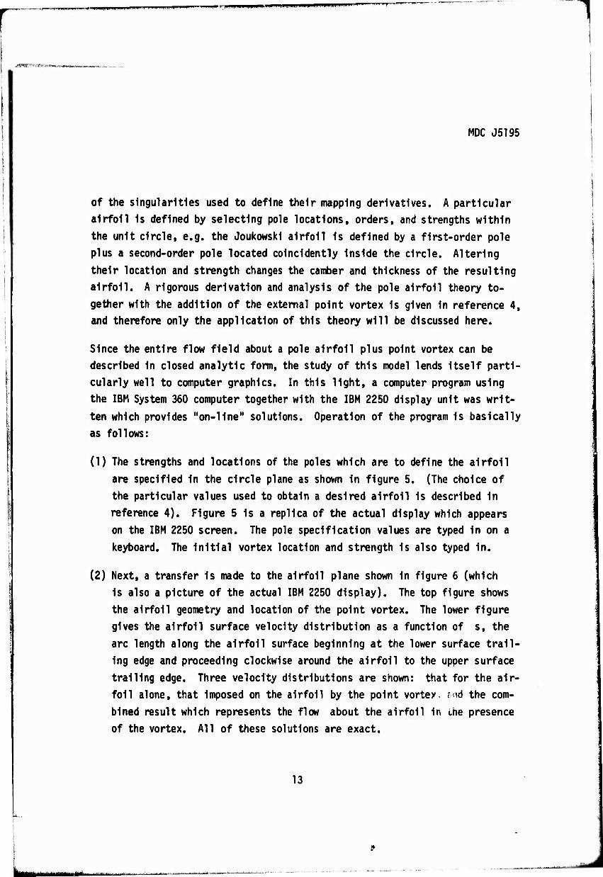
of the singularities used to define their mapping derivatives. A particular airfoil Is defined by selecting pole locations, orders, and strengths within

the unit circle, e.g. the Joukowskl airfoil is defined by a first-order pole

plus a second-order pole located colncldently inside the circle. Altering

their location and strength changes the camber and thickness of the resulting airfoil. A rigorous derivation and analysis of the pole airfoil theory to-

gether with the addition of the external point vortex Is given In reference 4, and therefore only the application of this theory will be discussed here.

Since the entire flow field about a pole airfoil plus point vortex can be described In closed analytic form, the study of this model lends Itself parti-

cularly well to computer graphics. In this light, a computer program using the IBM System 360 computer together with the IBM 2250 display unit was writ-

ten which provides "on-line" solutions. Operation of the program Is basically as follows:

(1) The strengths and locations of the poles which are to define the airfoil

are specified In the circle plane as shown In figure 5. (The choice of

the particular values used to obtain a desired airfoil Is described in

reference 4). Figure 5 Is a replica of the actual display which appears on the IBM 2250 screen. The pole specification values are typed In on a

keyboard. The Initial vortex location and strength Is also typed In.

(2) Next, a transfer Is made to the airfoil plane shown In figure 6 (which Is also a picture of the actual IBM 2250 display). The top figure shows

the airfoil geometry and location of the point vortex. The lower figure gives the airfoil surface velocity distribution as a function of s, the

arc length along the airfoil surface beginning at the lower surface trail-

ing edge and proceeding clockwise around the airfoil to the upper surface

trailing edge. Three velocity distributions are shown: that for the air- foil alone, that Imposed on the airfoil by the point vortex, <^d the com-

bined result which represents the flow about the airfoil In the presence

of the vortex. All of these solutions are exact.

13

" "Wl1 ! < ' I —r^—^^M ..... ui ■ » i i i ^n^wwiiiiimiii^i F-IIW."'! p i*

HOC JS195

(3) The airfoil angle of attack and the vortex strength and location can be

changed by merely keying In different values as desired. The results are

Immediately displayed on the IBM 2250 screen In the form of figure 6. At

any time the display may be printed for later reference which Is the

source of figures 5 and 6.

(4) The aerodynamic coefficients and parameters listed In figure 6 are defined

and related as follows:

ALPHA (a): Airfoil angle of attack as measured from the chord line.

CL (CL): Lift coefficient of the airfoil alone at that angle of attack.

CL TOTL (CL-): Lift coefficient of the total system (airfoil plus vortex).

CL AIRF (Cu): Lift coefficient of the airfoil In the presence of the vortex.

DEL CL (ACL): Specified Increment of lift for the total system (airfoil plus vortex) over the lift of the airfoil alone, i.e.

CLT - CL + ACL (1)

CD AIRF (CQ ): Drag coefficient of the airfoil In the presence of the

vortex. (Drag on the vortex Is equal and opposite to that of the

airfoil.)

RADIUS, THETAV (rv, öv): Location of the vortex In the circle plane.

An effective "slat" lift coefficient Is defined by

C, » C. -C. (2) LS LT LA

All of the aerodynamic coefficients are based on the airfoil chord and the

free stream velocity, V^. This Is more or less standard In multi-

element airfoil work, and allows convenient relations such as those given

by equations (1) and (2).

14

ia

j MM.--

.<&■>•' .■

MDC J5195

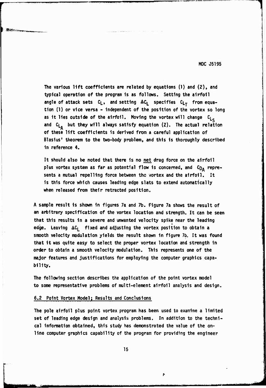
The various lift coefficients are related by equations (1) and (2), and

typical operation of the program Is as follows. Setting the airfoil

angle of attack sets (4» and setting AC|_ specifies Cu- from equa- tion (1) or vice versa - Independent of the position of the vortex so long

as It lies outside of the airfoil. Moving the vortex will change C|_

and CL but they will always satisfy equation (2). The actual relation

of these lift coefficients is derived from a careful application of

Blaslus* theorem to the two-body problem, and this Is thoroughly described

In reference 4.

It should also be noted that there Is no net drag force on the airfoil plus vortex system as far as potential flow Is concerned, and CQ. repre-

sents a mutual repelling force between the vortex and the airfoil. It is this force which causes leading edge slats to extend automatically

when released from their retracted position.

A sample result is shown In figures 7a and 7b. Figure 7a shows the result of an arbitrary specification of the vortex location and strength. It can be seen

that this results in a severe and unwanted velocity spike near the leading edge. Leaving AC^ fixed and adjusting the vortex position to obtain a

smooth velocity modulation yields the result shown in figure 7b. It was found

that it was quite easy to select the proper vortex location and strength in order to obtain a smooth velocity modulation. This represents one of the

major features and justifications for employing the computer graphics capa-

bility.

The following section describes the application of the point vortex model

to some representative problems of multi-element airfoil analysis and design.

6.2 Point Vortex Model; Results and Conclusions

The pole airfoil plus point vortex program has been used to examine a limited

set of leading edge design and analysis problems. In addition to the techni-

cal Information obtained, this study has demonstrated the value of the on- line computer graphics capability of the program for providing the engineer

15

""i" ' ' immmm « iimm^m^mmm*mmmmm!**immm*!*i**'m***l*r*w^m9,miw,[*m

MDC J5195

with a basic Intuition regarding leading edge slat performance. This same

Intuition could be obtained without using computer graphics, and Instead

running a variety of cases and then reducing the data to provide similar re- sults. However, the efficiency and vividness provided by the graphics capa-

bility appears to justify Its use.

The example problems which follow are Intended to demonstrate the capability

of the pole airfoil plus point vortex program and evaluate the point vortex

as a theoretical model for a leading edge slat. They should not be regarded

as a comprehensive study of all of the possible applications of the program. Many potentially Interesting problems have been left unexplored - due pri-

marily to the limited time available for this study.

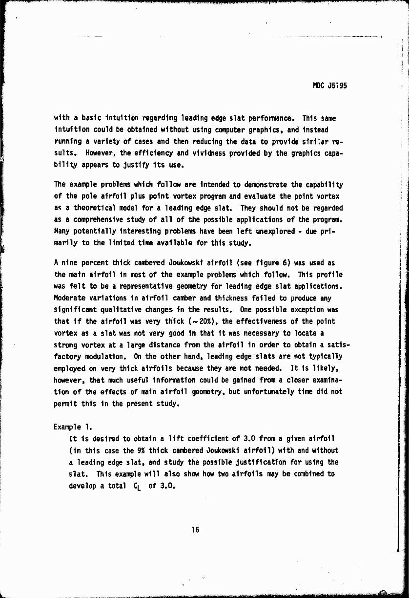
A nine percent thick cambered Joukowskl airfoil (see figure 6) was used as

the main airfoil In most of the example problems which follow. This profile was felt to be a representative geometry for leading edge slat applications.

Moderate variations In airfoil camber and thickness failed to produce any significant qualitative changes In the results. One possible exception was

that If the airfoil was very thick (~20%)( the effectiveness of the point

vortex as a slat was not very good In that It was necessary to locate a

strong vortex at a large distance from the airfoil In order to obtain a satis- factory modulation. On the other hand, leading edge slats are not typically

employed on very thick airfoils because they are not needed. It Is likely,

however, that much useful Information could be gained from a closer examina-

tion of the effects of main airfoil geometry, but unfortunately time did not

permit this In the present study.

Example 1. It Is desired to obtain a lift coefficient of 3.0 from a given airfoil

(In this case the 9% thick cambered Joukowskl airfoil) with and without

a leading edge slat, and study the possible justification for using the

slat. This example will also show how two airfoils may be combined to

develop a total C^ of 3.0.

16

i \

- i ii mimummtmt^mam^a^ltmUimWtat

MDC J5195

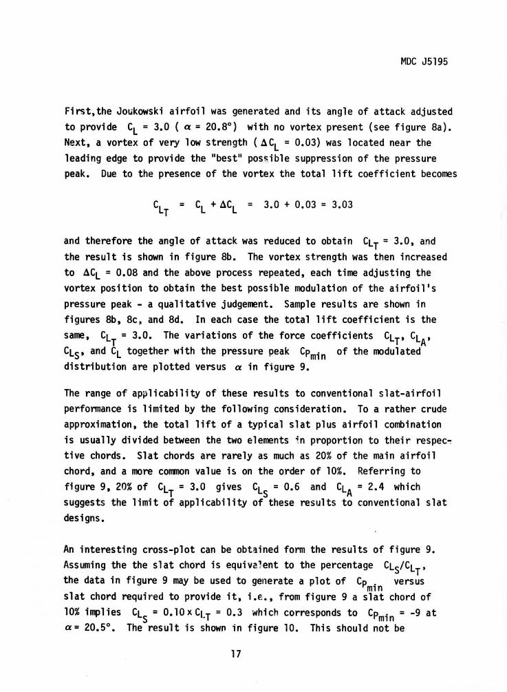
First,the Joukowski airfoil was generated and its angle of attack adjusted to provide CL = 3.0 ( a= 20.8°) with no vortex present (see figure Sa). Next, a vortex of very low strength ( ACL = 0.03) was located near the leading edge to provide the 11 best 11 pos~ ible suppression of the pressure peak. Due to the presence of the vortex the total lift coefficient becomes

CLT = CL +ACL = 3.0 + 0.03 = 3.03

and therefore the angle of attack was reduced to obtain CLT = 3.0, and the result is shown in figure 8b. The vortex strength was then increased to ACL = 0.08 and the above process repeated, each time adjusting the vortex position to obtain the best possible modulation of the airfoil's pressure peak - a qualitative judgement. Sample results are shown in figures 8b, Be, and 8d. In each case the total lift coefficient is the same, CLT = 3.0. The variations of the force coefficients CLT' CLA' Cls• and CL together with the pressure peak Cpmin of the modulated distribution are plotted versus a in figure 9.

The range of applicability of these results to conventional slat-airfoil performance is limited by the following consideration. To a rather crude approximation, the total lift of a typical slat plus airfoil combination is usually divided between the two elements in proportion to their respec~ tive chords. Slat chords are rarely as much as 20% of the main airfoil chord, and a more common value i5 on the order of 10%. Referring to figure 9, 20% of CLT = 3.0 gives cls = 0.6 and CLA = 2.4 which suggests the limit of applicability of these results to conventional slat designs.

An interesting cross-plot can be obtained form the results of figure 9. Assuming the the slat chord is equiva~ent to the percentage CLsiCLT' the data in figure 9 may be used to generate a plot of Cp . versus

m1n slat chord required to provide it, i.e., from figure 9 a slat chord of 10% i111Jl ies CL = 0.10 x Ct T = 0.3 which corresponds to Cp . = -9 at s · m1n a= 20.5°. The result is shown in figure 10. This should not be

17

IMIIPWPjIWWW^iPWffW.).) I|,l|l IllHWPWWpWIWWHIimi I ,ll||| Hill. Il ■,! lllll^mMWHI liiipmi-l

MDC J5195

regarded as a precise analytic fact, but rather as a qualitative Indica-

tion of the relation between Cp^ and the slat chord required to obtain

It. It can be seen that a slat chord on the order of 10% of the main air-

foil chord provides a very substantial reduction In Cpm1n. Increasing

the slat chord beyond about 15% produces a relatively small reduction in

CPm1n-

Example 2.

Here It Is desired to Increase Ci while holding Cp 4 on the airfoil

to a specified value which might be set by separation criteria. Again, a

9% thick cambered Joukowskl airfoil was used. First, the airfoil angle

of attack was set so that Cpm^n reached the specified value with no

vortex present. The angle of attack was then Increased by a few degrees

and the vortex strength and position adjusted so that Cpn|1n was reduced

to the specified value using the minimum possible vortex strength. This

process was then repeated until the airfoil angle of attack reached 45°

which Is somewhat beyond the range of practical operation. Sample results

are shown In figures 11a, lib, and lie. The resulting variations of the

various lift coefficients are shown In figures 12 and 13 for specified

values of Cp j of -8 and -12 respectively. Also shown Is the Implied

slat chord based on the ratio CLS/CLT as In Example 1. Using this data,

a cross plot of Cu- versus the Implied slat chord required to obtain It

was made and Is shown In figure 14 for both Cp^ « -8 and Cpm1n = -12.

One of the cruder forms of boundary layer separation criteria says that the

existence of attached flow Is dependent on some maximum (numerical) value

of Cp^ which lies somewhere between -8 and -12. A pressure peak which Is

higher Is likely to cause separation - possibly of the entire upper surface

of the airfoil since the peak Is located near the nose. Therefore, figures

12 and 13 may be regarded as demonstrating the ability of a slat to Increase

the CL(nax of an airfoil. Alternatively, these results demonstrate the abil-

ity of a slat to Increase the angle of attack range of an airfoil. Figure

14 shows that the slat chord required varies effectively linearly with the

Increase In CLT, and figures 12 and 13 show that the slat chord varies al- most linearly with a.

18

■ ii -•- •- M—■ ^^^M^MMMHMlMMMMMHMlflililBMi

im r iw»»»!—WWW—W mmm

WiKim»*

MDC J5195

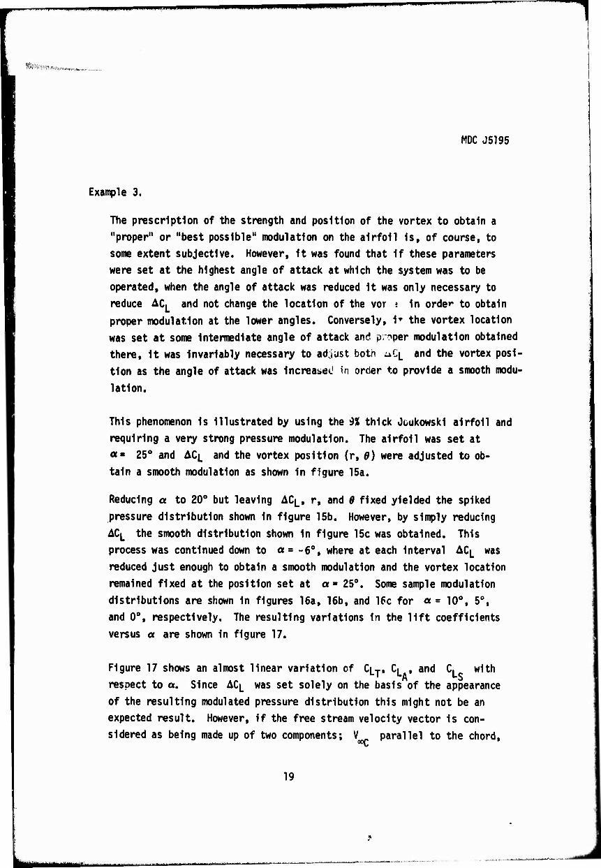
Example 3.

The prescription of the strength and position of the vortex to obtain a

"proper" or "best possible" modulation on the airfoil Is, of course, to

some extent subjective. However, It was found that If these parameters

were set at the highest angle of attack at which the system was to be

operated, when the angle of attack was reduced It was only necessary to

reduce AC^ and not change the location of the vor ; In order to obtain

proper modulation at the lower angles. Conversely, 1* the vortex location

was set at some Intermediate angle of attack and proper modulation obtained

there. It was Invariably necessary to adjust both üCL and the vortex posi-

tion as the angle of attack was Increased in order to provide a smooth modu-

lation.

This phenomenon Is Illustrated by using the 9% thick Joukowskl airfoil and

requiring a very strong pressure modulation. The airfoil was set at

«= 25° and ACL and the vortex position (r, d) were adjusted to ob- tain a smooth modulation as shown In figure 15a.

Reducing a to 20° but leaving ACL, r, and 9 fixed yielded the spiked pressure distribution shown In figure 15b. However, by simply reducing

ACL the smooth distribution shown In figure 15c was obtained. This

process was continued down to a= -6°, where at each Interval AC|_ was

reduced Just enough to obtain a smooth modulation and the vortex location

remained fixed at the position set at a- 25°. Some sample modulation

distributions are shown In figures 16a, 16b, and 16c for a = 10°, 5°,

and 0°, respectively. The resulting variations In the lift coefficients

versus a are shown In figure 17.

Figure 17 shows an almost linear variation of CLT, CL , and CL with

respect to a. Since AC^ was set solely on the basis of the appearance

of the resulting modulated pressure distribution this might not be an

expected result. However, If the free stream velocity vector Is con-

sidered as being made up of two components; V,, parallel to the chord,

19

«M^ mmmmmmm mm

MDC J5195

and Va)N normal to the chord, a simple explanation can be offered. For small a, V(

called "cross-flow component of velocity"

edge pressure peak on the airfoil.

^ Is nearly directly proportional to a, and It Is the so-

VCQI^I which causes the leading

Therefore since 1^ varies approxi- mately linearly with a,and the Intensity of the pressure peak does like-

wise. It Is not surprising that the strength of the vortex required to

suppress the peak also varies linearly with a.

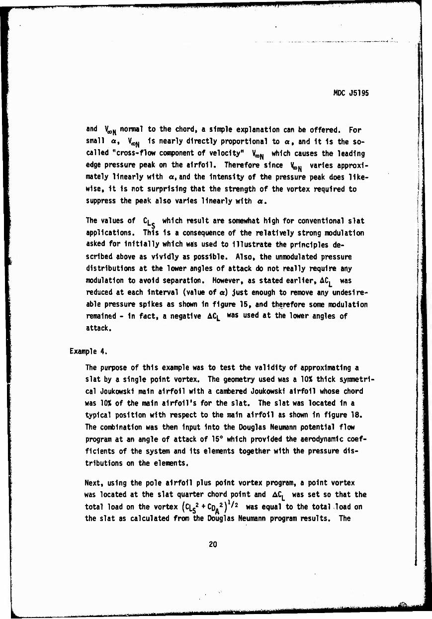
The values of C|_ which result are somewhat high for conventional slat

applications. This Is a consequence of the relatively strong modulation asked for Initially which was used to Illustrate the principles de-

scribed above as vividly as possible. Also, the unmodulated pressure distributions at the lower angles of attack do not really require any

modulation to avoid separation. However, as stated earlier, AC. was

reduced at each Interval (value of a) Just enough to remove any undeslre-

able pressure spikes as shown In figure 15, and therefore some modulation remained - In fact, a negative AC^ was used at the lower angles of

attack.

Example 4.

The purpose of this example was to test the validity of approximating a slat by a single point vortex. The geometry used was a 10% thick symmetri- cal Joukowskl main airfoil with a cambered Joukowskl airfoil whose chord was 10% of the main airfoil's for the slat. The slat was located In a typical position with respect to the main airfoil as shown In figure 18.

The combination was then input Into the Douglas Neumann potential flow program at an angle of attack of 15° which provided the aerodynamic coef- ficients of the system and Its elements together with the pressure dis- tributions on the elements.

Next, using the pole airfoil plus point vortex program, a point vortex was located at the slat quarter chord point and ACL was set so that the

total load on the vortex (CLC2 + CDA2) ^2 was equal to the total load on

the slat as calculated from the Douglas Neumann program results. The

»,

20

m «nur mm iiimiMii ■Ma> MHJto (MM

■ .■n pi i Ri^iiwpn mmmm M 'r1*"»» P^

MDC J5195

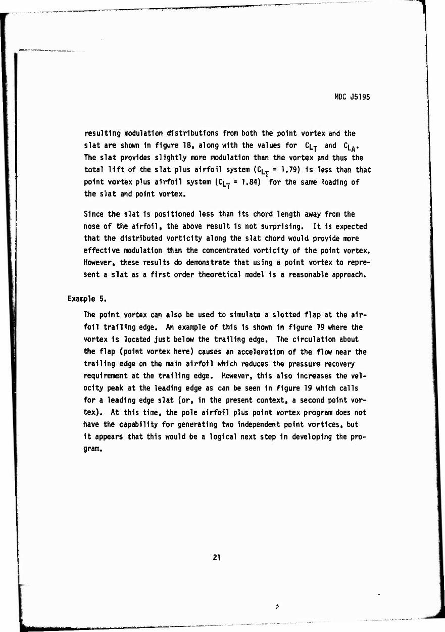
resulting modulation distributions from both the point vortex and the

slat are shown In figure 18, along with the values for CL-T and Cu«

The slat provides slightly more modulation than the vortex and thus the

total lift of the slat plus airfoil system (CLT = 1.79) Is less than that

point vortex plus airfoil system (CLT = 1.84) for the same loading of the slat and point vortex.

Since the slat Is positioned less than Its chord length away from the

nose of the airfoil, the above result Is not surprising. It Is expected that the distributed vortlclty along the slat chord would provide more

effective modulation than the concentrated vortlclty of the point vortex. However, these results do demonstrate that using a point vortex to repre-

sent a slat as a first order theoretical model Is a reasonable approach.

Example 5.

The point vortex can also be used to simulate a slotted flap at the air-

foil trailing edge. An example of this Is shown In figure 19 where the

vortex Is located just below the trailing edge. The circulation about

the flap (point vortex here) causes an acceleration of the flow near the

trailing edge on the main airfoil which reduces the pressure recovery requirement at the trailing edge. However, this also Increases the vel-

ocity peak at the leading edge as can be seen In figure 19 which calls

for a leading edge slat (or. In the present context, a second point vor-

tex). At this time, the pole airfoil plus point vortex program does not have the capability for generating two Independent point vortices, but

It appears that this would be a logical next step In developing the pro- gram.

21

*m ■■■ ii ■ mmmmmmmmmmm^^mmmmtfimi***1***^^** vmm

NDC J5195

7.0 DISTRIBUTED SINGULARITY MODEL

7.1 General Discussion

As mentioned in the Introduction, a next level of sophistication beyond the

point vortex model appears to be the representation of the slat by a contin- uous distribution of singularities along the slat chord. The use of thin

airfoil theory for describing the slat and its effect on the main airfoil is

particularly appealing from the standpoint that linearized theory allows the separation of camber and thickness, and moreover, the theory is quite simple

and straightforward when compared with the exact solution formulation. Since, as discussed earlier, the exact goals of slat analysis and design theory

are not completely clear, it is felt that a linearized analysis should be

conducted in order to provide proper guidance for an exact solution study.

It may be recalled that much of the fundamental information regarding the performance of single element airfoils comes directly from thin airfoil theory.

The basic "new" analytical problem of using thin airfoil theory to represent the slat is the determination of an appropriate system of imaging the slat

singularity distributions so that the presence of the main airfoil Is pro-

perly accounted for. At first, it appeared that an extension of the point

vortex model to the case of distributed vorticity along a slat chord line might be the best approach to use. However, examination of the method devel-

oped by O'Pray in reference 4 suggested that continued development and eval-

uation of his work would probably be the most fruitful course to follow.

Since the available documentation of O'Pray's method was rather limited, it

was first necessary to redevelop his entire analysis here at Douglas. Also,

O'Pray obtained his sample solution using an on-line computer facility which allowed him to directly interact with the calculation procedure and adjust

various inputs and parameters until a satisfactory result was obtained. There- fore it was decided to develop a new computer program which would minimize

22.

--• '-—'—'—^—^-^-^

MDC J5195

if not eltminate any requirements for "man-in-the-loop" interaction. It is stressed that the above comments should in no way be interpreted as a criti­cism of O'Pray•s work. Instead, his synthesis and formulation of the lead­ing edge slat design problem was regarded as sufficiently impressive that further development was definitely in order. The discussion which follows is intended as a detailed description but not a rigorous development of O'Pray•s method.

The problem to be solved is that of designing a leading edge slat which pro­vides a specified pressure distribution modulation on the nose region of the main airfoil. As stated, this problem is somewhat underspecified and it is not likely to possess a unique solution. Therefore some additional conditions may be imposed. The use of thin airfoil theory implies representing the slat by an infinite set of singularity distributions whose coefficients are to be set on the basis of the boundary conditions which are to be satisfied. The pressure field imposed on the main airfoil by these singularity distributions is linear with respect to the magnitude of their coefficients and nonlinear with respect to the location of the slat chord. Thus it seems reasonable, at least to begin with, to specify the slat chord position, and then attempt to determine the proper values for the mode coefficients. The choice of the coefficients involves two basic requirements: (1} they must provide the desired pressure distribution mudulation on the main airfoil, and (2} they must correspond to a real and useable geometry for the slat itself. (There is no a priori guarantee that an arbitrarily chosen set of mode coefficients might not imply a slat of negative thickness or one whose trailing edge does not close.}

One of the major features of O'Pray•s method lies in the choice of the various conformal mappings employed. Instead of working with an arbitrary main air­foil shape, an ellipse of arbitrary thickness is used. It is observed that for most conventional airfoils without extreme leading edge camber or nose droop, the nose region itself i s very nearly elliptical, and therefore the nose flow about an ellipse closely models the typical flow environment of a leading edge slat. Thus an ellipse with its circulation set to maintain the Kutta condition

23

^^mmfmmmmmmmKmmmHitß Km mmumim

MDC JS195

at Its trailing edge becomes a rather Ideal model for a main airfoil to study

slat performance since its mapping to a circle Is straightforward.

7.2 Description of Analysis.

A. Mapping functions.

Several consecutive mappings are used In the analysis beginning with the mapping from the ellipse (z (xi» y^)-planet figure 20a) to the circle

(z (xg, y2)-plane, figure 20b) where the mapping function Is given by

z + C7/42

1 /2[z + (Z2 -c;)1^] (3)

where c, a a2 - b2 and a and b are the major and minor axes of the ellipse. The radius c, of the corresponding circle in the z-plane Is ob-

tained from C3 ■ (a + b)/2. Next, the circle Is opened at Its trailing edge and Is mapped to the real axis of the half-plane (M^, y3)-plane,

figure 20c) where ya > 0 corresponds to that region outside the circle.

The point at Infinity In the z-plane maps to y3 » 1 In the W-plane, and

the leading edge maps to the origin while the leading edge stagnation point

maps to a small value of - X3 on the negative real axis (If the angle of

attack of the ellipse Is zero, the stagnation point and the leading edge become coincident). The mapping from the circle-plane to the half-plane Is

W R) (4)

The geor.

re«1* :, i^

lih.i 0.

ie« of these mappings are shown In figure 20, where the modulation Indicated by the heavy line. Also shown In figure 20c are the stream-

iie flow near the leading edge. It Is observed that in the near vicinity of the modulation region the curvature of the streamlines Is rather

24

L_ MMMM

m ." WWWW >KW»>»pl«li"«W»"»

MDC J5195

moderate, and therefore a straight line slat chord may be placed tangent to

one of the streamlines as shown In figure 20c. The selection of a particular

slat chord position Is based on the location, extent, and character of the

desired modulation distribution. This will be discussed In greater detail

later.

Once the slat chord position Is set, a simple mapping to the slat-centered half-plane (s (s,t) - plane) Is made, where the origin iof the S-plane

lies at the slat mldchord and the real axis parallels the slat chord as shown in Figure 20c. This mapping Is merely a translation plus rotation plus dila-

tion and Is given by

i- >s w -(vS) (5)

where f2 and f^ are the coordinates of the slat mldchord, a$ Is the slat angle with respect to the x3-ax1s, and cs Is the slat chord length - all

measured In the W -plane. Since 1t has been assumed that the slat chord will

be set tangent to the local streamline which determines a , only the three

parameters f^ f2, and cs are needed to specify the slat. In the S-plane,

the slat chord runs from s = -2 (the slat leading edge) to s = +2 (the slat

trailing edge)*. This completes the mappings used In the analysis.

The main appeal of the above set of mappings lies In the fact that when a

singularity distribution Is defined on the slat chord, an Identical singular-

ity distribution may be defined on an Image slat chord located as shown In

figure 20c. This Is the same procedure used for analyzing a conventional air-

foil In ground effect where the ground surface becomes the axis of symmetry

of the potential flow field. The fact that the main flow field In the W -

plane Is not a uniform stream does not affect this model. In the analysis

which follows, the X3 - axis of the W-plane (which is actually the surface

*A slat chord of 4 Is convenient In defining the singularity distributions.

25

IIBlfnli.. II in1"-'

*w "—'■ M-I.-M i i iimtiiitrfmmmmvmmF'mm^inwnii^fflll^nm'^^rm^mri if fuii\m~<Mmmm,,iium , i|i-" unim ■I"«-VF'FV'—r» .T»".- - i"^|

MDC J5195

of the ellipse), will often be referred to as the "ground plane" In analogy to the above.

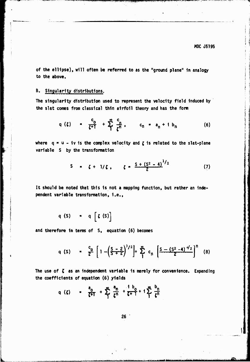
B. Singularity distributions.

The singularity distribution used to represent the velocity field Induced by

the slat comes from classical thin airfoil theory and has the form

q ({) _oo C

FT 1 {n an + 1 bn (6)

where q > u - iv Is the complex velocity and ( Is related to the slat-plane

variable S by the transformation

Vs . {+ 1/c. c. sMf-4)^ (7)

It should be noted that this Is not a mapping function, but rather an Inde- pendent variable transformation. I.e.,

q (S) - q [{ (S)]

and therefore In terms of S, equation (6) becomes

q (S) co 7"

Vj [,-(^),/2j+Ecn[i^llIi in

(8)

The use of C as an Independent variable Is merely for convenience. Expanding the coefficients of equation (6) yields

q (0 - ^r + E jn rn-+i^ jn

26

..^■^..-y-^... \tm —■■■■ ■■■■- BMBI i __.. -^ - .IIM^IHIMI >■■ r ■>!■■ i mii^iiiii ii inn ■n^MMiiatfll

•^^^m-^mmmi wpwywii —IP»» »■mill»' 7n—Miiiii

WWW'Milf

MOC J5195

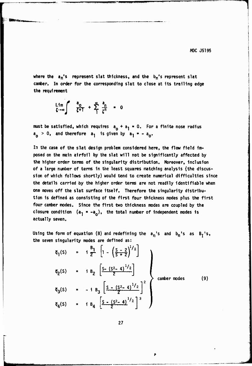
where the a^s represent slat thickness, and the bn's represent slat

camber. In order for the corresponding slat to close at Its trailing edge

the requirement

Lim f ao 00

1 cn

must be satisfied, which requires a0 + a1 « 0. For a finite nose radius a. a > 0, and therefore a-j Is given by a-j = - a0.

In the case of the slat design problem considered here, the flow field Im-

posed on the main airfoil by the slat will not be significantly affected by

the higher order terms of the singularity distribution. Moreover, Inclusion of a large number of terms In the least squares matching analysis (the discus- sion of which follows shortly) would tend to create numerical difficulties since

the details carried by the higher order terms are not readily Identifiable when

one moves off the slat surface Itself. Therefore the singularity distribu-

tion Is defined as consisting of the first four thickness modes plus the first

four camber modes. Since the first two thickness modes are coupled by the closure condition (a-j - -a0), the total number of Independent modes Is

actually seven.

Using the form of equation (8) and redefining the a^s and bnls as Bj's,

the seven singularity modes are defined as:

VS)

1B2

- 1 B.

1 B,

[ - MV2] S- ($2- 4)1/21 ^ j

S - (S2- 4)^2] 1 L T J

^ü1/2]3

camber modes (9)

27

IMI! ., iiiMiippW)ui|i..iiipiiiiwi||ir^^ . iipiniiw. mi ,ii|i»niii|ii.jilil|iiuyfii.i.il.,.P.^.,y,l. .,.

MDC J5195

qs(S)

%&

q7(S)

IS-2\1/2' S-(S2 - 4)1/2 i: -B S - (S2- 4)

B6 ^T—^

l/2

'thickness modes (9)

BJs-iSiV/2 n3

The corresponding slat geometry mode shapes are sketched In figure 21, and

the velocity distribution of equation (6) becomes

q(S) £ ^l(S) - g B1 qi(S)

In terms of S. The complex velocity In the half plane q (W) Is given by

q(W) - q(S)^ - q(S)5-eias (10)

where dS/dW Is obtained from equation (5). Now the real and Imaginary parts

of q(W) on W = x3 (y3 s 0) represent the parallel and normal slat singular-

ity Induced velocities on the ground plane (I.e. the ellipse surface In the

W-plane). Defining

qI(S) - uI(S)-1 VjfS)

qjCW) - UjOO-l v^W)

and using equation (10) yields

UI(W) a f" UI(S) cos as * vl^s) s1n «s

Vjd^) - - i- ^(S) sin as - v^S) cos as

(11)

28

i (i i -MI i ltort^M)lMiaMMg,MMiail|MiMjB||||iaMiiiWiBilii itmmm*a*

.-1—«WTf—W"-*»-

.,CT,.,..„,IIPI.WJIHHIIIIHI niiumpiiiipjmiii iifiiniji i i i —^»w—^^^W!^ ■RÜMR

MDC J5195

as the components of the velocity Induced In the W-plane (half-plane) by

each of the I singularity modes, where the Uj(S) and Vj(S) are known from the expressions given by equations (9).

Since an Image slat Is located In the lower half of the W-plane, the X3-

axls becomes an axis of symmetry, and on the X3 - axis the total velocity Induced by the slat plus Image slat singularity distributions Is simply

"(x,) 1=1

BI UI ^ (12)

where the ^(W) are defined by equations (11), and are functions of the

slat chord and Its position In the W-plane only. The factor 2 is due to the presence of the Image slat.

C. Determination of the mode coefficients.

The problem remains to determine the coefficients B, of the singularity

distribution modes so that the Induced velocity u(x~) provides the desired

modulation on the ground plane (I.e. on the nose region of the ellipse). Typi-

cally the desired velocity modulation will be specified by a set of values at

a finite number of discrete points along the ellipse nose surface. This

specified velocity Is readily mapped to the half-plane where It Is defined as

w(x3i) w1» 1=1,2, —, L (number of matching stations)

where the x^ are the matching stations. Next, comparing the desired

velocity with that Induced by the singularity distributions yields the L-equätlons

Oi w(x.J -2 £ B, u (x-J. 1 = 1, L ^31 J=l J J ^31

or wi-2 S B*"" . 1 = 1. L

29

mm 1 11 in u^ma^Mjiig rriM-

■"■■' ■- —■■— niiiniimiuiiiii, 111WH.W WP^ff^WBPPW uppt^wppniiiiipi .ivi|i|i ii um i ii

MDC J5195

The tenns \x^ are called "influence coefficients" and are defined as the

velocity on the ground plane at the matching station x.j Induced by the Jth singularity mode with a unit mode coefficient.

The values of the mode coefficients B, are determined using a standard least squares matching procedure. Letting

0 1=1 1

and differentiating ^ with respect to the B, yields

^"^^■2s("i-i^)N or % uJi «1 = 0» J= 1. —. 7 (13)

as seven simultaneous equations to be solved for the seven mode coefficients Bj. In matrix notation, equations (13) become

u (w - u B) e n (14)

where the matrices of equation (14) are defined by

B

uji 1 J x ^ octangular matrix

I w1

i öJ

■ 1 column matrix

• J column matrix

30

mäit±*ta±Mmta*mm*i iiii'iiiii'aniiiiii-""'--^--^^^'"^ mm ittMM

MDC J5195

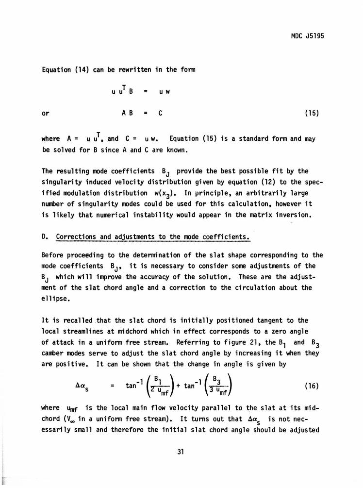
Equation (14) can be rewritten in the form

= u w

or A B = C ( 15)

where A = u uT, and C = u w. Equation (15) is a standard form and may be solved for B since A and C are known.

The resulting mode coefficients BJ provide the best possible fit by the singularity induced velocity distribution given by equation (12) to the spec­ified modulation distribution w(x3). In principle, an arbitrarily large number of singularity modes could be used for this calculation, however it is likely that numerical instability would appear in the matrix inversion.

D. Corrections and adjustments to the mode coefficients.

Before proceeding to the determination of the slat shape corresponding to the mode coefficients BJ, it is necessary to consider some adjustments of the BJ which will improve the accuracy of the solution. These are the adjust­ment of the slat chord angle and a correction to the circulation about the ellipse.

It is recalled .that the slat chord is initially positioned tangent to the local streamlines at midchord which in effect corresponds to a zero angle of attack in a uniform free stream. Referring to figure 21, the s1 and s3 camber modes serve to adjust the slat chord angle by increasing it when they are positive. It can be shown that the change in angle is given by

= (16)

where Umf is the local main flow velocity parallel to ~he slat at its mid­chord (V~ in a uniform free stream). It turns out that ~as is not nec­essarily small and therefore the initial slat chord angle should be adjusted

31

w,..—yw^^wnWi—f »■■■■"»I r»"'. M-IWHf "* vm 'ff1 '"'■ T-(W<WP«l| I i 1

MDC J5195

accordingly. This changes the values of the Influence coefficients and there-

fore a repeat of the least squares solution Is required to obtain a refined

set of mode coefficients Bj. Repeating this procedure again Is not Justified on the basis of the Inherent accuracy of thin airfoil theory.

Another correction arises due to the Image slat vortlclty. When mapped back

to the ellipse plane, the Image slat lies Inside the ellipse and Its vortlclty

due to the camber modes Bj, Bp, By and B4 moves the rear stagnation point

and the Kutta condition Is no longer satisfied. The Image slat circulation Is calculated by considering the problem In the circle plane. Most of the

slat vortlclty Is contained In the Bj and B» terms, and the B. and B.

terms can be neglected within the accuracy of thin airfoil theory. The vor-

tlclty of the Bj and Bp terms 1s approximated by a point vortex of strength

ZirB^ at the slat quarter chord and a point vortex of strength 2irB2 at the

slat mldchord. The corresponding Image locations and circulation correction

required to maintain the Kutta condition Is then calculated In the circle plane using the same method as was employed In the point vortex model.

Even though the ellipse circulation correction amounts to less than one percent

of the total ellipse circulation. It causes a significant change In the ellipse

pressure distribution, particularly In the nose region. As a result the spec-

ified modulation velocity distribution w(x3) changes and therefore a new

least squares solution Is necessary. Due to the sensitivity of the nose flow to the ellipse circulation this procedure Is repeated. Convergence to a negli-

gible correction occurs after three or four cycles.

E. Slat thickness constraints.

Thus far 1n ths analysis the calculation of the mode coefficients has been

based almost solely on the requirement that they provide the desired velocity

modulation distribution on the nose of the ellipse. It now becomes necessary

to identify some geometrical considerations - In particular with respect to the

slat thickness distribution. Earlier In the analysis closure of the slat was

guaranteed by setting a1 = - a0. This does not, however. Insure that the

32

lit,-- ii i ■ numt"'■■■•• ■ • ■■'-■ -

MDC J5195

thickness mode coefficients 85, 86, and 87 as chosen by the least squares solution won•t provide a slat thickness distribution which is re-entrant. In fact, it turns out that if the sciution is left unconstr~ined this is quite often what happens. Such a result is readily understood when it is recalled that the slat is called on to provide a velocity modulation which opposes the main flow on the ellipse. This is accomplished by the circulation generated by the slat, however, in many cases positive thickness will tend to reduce this effect by causing an acceleration of the flow.

This difficulty is overcome by simply removing the thickness mode coefficients from the least squares matching solution, and prescribing them to provide any thickness distribution desired. The only modification required for the least squares solution is that the differences 8i become

where wt(x3i) represents the velocity induced on the ground plane at x3i by the prescribed slat thickness distribution, and of course there are only 81, 82, 83, and 84 (the camber ~de coefficients) to be determined. It is convenient, but not necessary, to specify the thickness distribution by select­ing values of 85, 86, and 87, however any desired thickness distribution is in principle admissible.

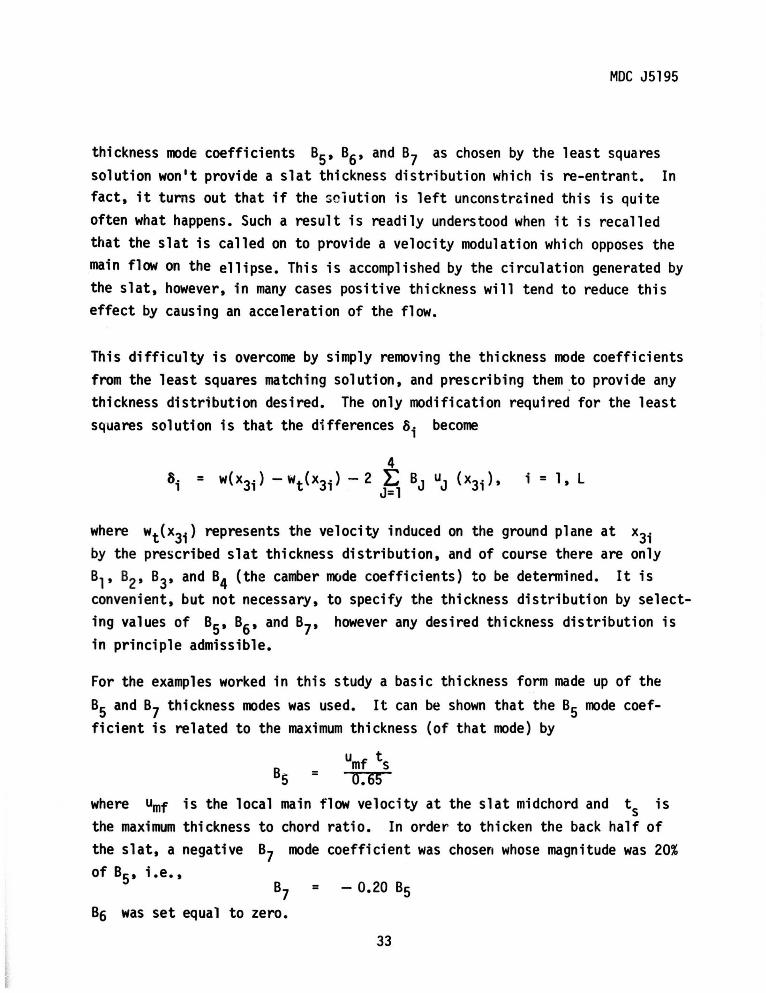
For the examples worked in this study a basic thickness form made up of the 85 and 87 thickness modes was used. It can be shown that the 85 mode coef­ficient is related to the maximum thickness (of that mode) by

umf ts = 0.65

where umf is the local main flow velocity at the slat midchord and ts is the maximum thickness to chord ratio. In order to thicken the back half of the slat, a negative 87 mode coefficient was chosen whose magnitude was 20% of 85, i.e.,

= - o.2o 85 86 was set equal to zero.

33

w. wmmm —m WilWWPiWW|WWIWW|P^wwEFip lfcWl.11""' PPMPW^P ' , mmmmmmm "i *

MDC J5195

The apparent necessity for prescribing the thickness distribution Is not as

bad as It may seem at first. In design problems, structural considerations

often dictate thickness distribution requirements. The ability to specify

the thickness distribution then allows an additional degree of freedom In the slat design problem since the camber distribution will then be calculated

to provide the desired velocity modulation using the given thickness distribu- tion.

F. Determination of slat geometry.

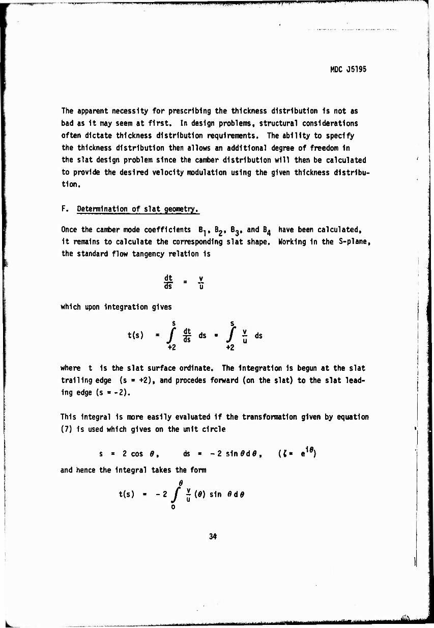
Once the camber mode coefficients B-., I^» B3, and 8^ have been calculated, It remains to calculate the corresponding slat shape. Working In the S-plane, the standard flow tangency relation Is

dt a v 3s "u

which upon Integration gives

t(s)

+2 +2

where t Is the slat surface ordlnate. The Integration Is begun at the slat

trailing edge (s ■ +2), and precedes forward (on the slat) to the slat lead- ing edge (s « -2).

This Integral Is more easily evaluated If the transformation given by equation

(7) Is used which gives on the unit circle

s «• 2 cos 9, ds - ~2s1n0d0,

and hence the Integral takes the form

6

t(s) = -* f lW s1n 0(ie

U- e1*)

34

■ ....— - 1 -■■-"■"—■—-»'■'■■"■■ ni iiiiüttiliili MMMMii

•mmmmm^mrniBl

^mtmmmmm^.

MDC J5195

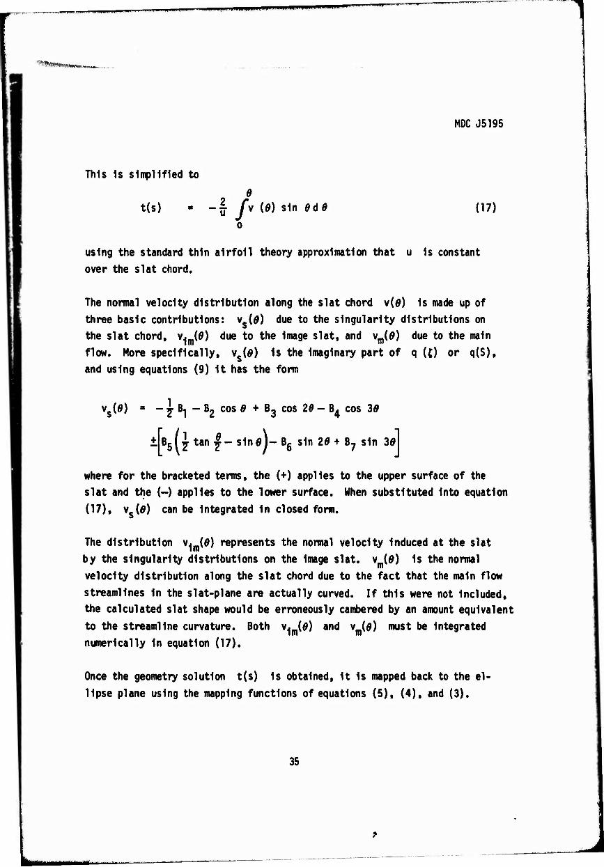
This Is simplified to

t(s) -f /v(*) sin edd (17)

using the standard thin airfoil theory approximation that u Is constant

over the slat chord.

The normal velocity distribution along the slat chord v(0) Is made up of

three basic contributions: vc(^) due to the singularity distributions on

the slat chord, v4ni$) due to the Image slat, and 'Im VmO flow. More specifically, vs(^) Is the Imaginary part of

and using equations (9) It has the form

due to the main

q (() or q(S).

vs(*) - j- B1 - B2 cos ö + B3 cos 26 - B4 cos 30

±|B5f]-tan|-s1ntfj- Bg sin 2tf + B 7 sin 301

where for the bracketed terms, the (+) applies to the upper surface of the

slat and the (-) applies to the lower surface. When substituted Into equation

(17), vs(0) can be Integrated In closed form.

The distribution v<||n(0) represents the normal velocity Induced at the slat

by the singularity distributions on the Image slat, v (0) Is the normal

velocity distribution along the slat chord due to the fact that the main flow

streamlines In the slat-plane are actually curved. If this were not Included,

the calculated slat shape would be erroneously cambered by an amount equivalent

to the streamline curvature. Both v4m(0) and

numerically In equation (17).

,1mv vmW must be Integrated

Once the geometry solution t(s) Is obtained. It Is mapped back to the el-

lipse plane using the mapping functions of equations (5), (4), and (3).

35

L_

mmm mm m f""' wpw' iwilimi ^-^^—^^^—'^^^^— ^—,-,^-,

MDC J5195

G. Method of calculation.

In order to evaluate the Inverse slat design method Just described, a computer

program was written In Fortran IV language for the IBM System 360 computer. The required Input data Includes: the ellipse thickness ratio, the ellipse angle of attack, the desired pressure modulation distribution, the thickness dis-

tribution of the slat, the slat chord length cs, and the slat mldchord loca-

tion {f2, fi). The program selects the proper slat chord angle as and deter-

mines th? camber mode coefficients Bj, Bg, B3, and B4 which provide the

closest possible match to the desired pressure modulation distribution. These

calculations Include the corrections for Image Induced circulation on the

ellipse and slat chord angle. The resulting singularity distributions are then Integrated to obtain the slat geometry Including the necessary adjustments

for the presence of the Image slat and streamline curvature In the W-plane.

Finally, the resulting geometry Is mapped back to the ellipse plane to yield

the actual slat shape.

In Its present form, the program requires that the desired modulation distri- bution be Input as a function of the Z-plane variable X|, and of course

the Input variables c., fp and fg are defined In terms of W-plane coor-

dinates. This was done for the sake of expediency In order to be able to

evaluate the distributed singularity distribution model In the limited time

available. As a consequence, prescribing this input data is somewhat more

awkward than would be desirable - particularly for an individual with limited

experience. However, once this data has been specified, the calculation of

the slat geometry is completely automatic and requires no Interaction with a Hman-in-the-1oop". The computer time required for a complete run on a 360/65

computer is less than one tenth of a minute, and therefore iterating to obtain

a desired slat geometry is quite economical.

It should be noted that the program always yields a slat shape. However, if

inappropriate values of c , f^, or fg are specified, or an "impossible"

36

.—. ,.i.. Wi.i.nn. .. i...wui.i.i.-i.. ..-u»^...^^.....^,-.—rr — ^mm

MDC J5195

modulation Is sought, the resulting slat geometry will likely be rather pecu-

liar, and Its modulation distribution may not completely agree with the one

requested. Some sample results are presented In the following section.

7.3 Distributed Singularity Model; Results and Conclusions

The O'Pray Inverse slat design method has been applied to a limited set of

examples using the computer program developed In this study. These examples

are Intended to illustrate the basic viability of the method, and should not

be regarded as a comprehensive display of all possible applications.

The main airfoil ellipse used for all of the examples Is that chosen by O'Pray

for his single test case: a 14% thick ellipse which In turn has a nose radius

of about one percent of Its chord. The ellipse Is set at an angle of attack

of about 17.2° (actually 0.3 radians) which gives a lift coefficient of 2.12,

and a leading edge pressure peak of Cp = -22.7. A pressure distribution modulation Is specified which reduces this pressure peak to Cp * ■ -9. Fig-

ure 22 shows the pressure distribution on the nose region of the ellipse with- out modulation and that which results from the specified modulation distribu-

tion. (The other data shown In this figure will be explained shortly.) This

pressure peak and required modulation of It are quite severe, and thus should

represent a good test for the method.

The first problem considered was similar to O'Pray's test case: design a 10%

thick slat to provide the specified modulation. Using the basic thickness

distribution described In section 7.2E with ts s 0.10, the slat shown In

figure 23a was obtained. This slat geometry plus the ellipse was Input Into

the Douglas Neumann potential flow program and the modulated pressure distri-

bution provided by the slat Is plotted In figure 22. The resulting slat geo-

metry does not quite agree with that obtained by O'Pray, however, this result

Is not unexpected since his calculation routine was not the same as that of

the Douglas program.

37

aM—mM— ' — '— ■ mlll«mllllllHllllllim«ll ' ' ^-^^.^■^-^-^--^^^^-^^" mlri rliiiirilirtii

""t'i" -.' •«miw*wmmmmi*m'im*mmmrmm**im m.mm'i ,ii' mm tf nm.vKipi "TWI

MDC J5195

Next, the slat thickness was Increased to 15* by setting t - 0.15, and to

201 by setting ts « 0.20. The resulting slat geometries are shown In figures 23b and 23c, respectively, and the resulting modulated pressure distributions

as obtained from the Douglas Neumann program are shown In figure 22.

Finally, the ellipse angle of attack was Increased to a > 18.4° (0.32 radians)

which gives a lift coefficient of 2.3 (Cp^ ■ -25.7), and the same modulation

(Cpm1n ■ -9) requested. A 15X thick slat was called for and Its resulting geometry Is shown In figure 23d with the Douglas Neumann calculation of Its

corresponding modulated pressure distribution again plotted In figure 22.

The results shown In figures 22 and 23 Indicate that there Is no unique sol- ution to problem (b) as described In the Introduction, and thus there exists

a wide variety of slat geometries capable of accurately matching a specified pressure modulation distribution on the nose region of a given airfoil. This

means that some of the slat geometry parameters (e.g. the thickness distri-

bution) may be used to satisfy other constraints. These Include structural,

mechanical, and aerodynamic considerations. For example. It appears that It

should be possible to constrain the upper surface shape of the slat, and with a proper reformulation of the method obtain solutions to problem (a) described

in the Introduction. Similarly,It Is possible that the method could be ex- tended to handle the design problem where the upper surface velocity distri-

bution would be constrained to avoid boundary layer separation on the slat

Itself. Unfortunately, the limited time available for this study did not

permit such further Investigations.

On the basis of the limited application and results obtained, the distributed singularity model as developed by O'Pray In reference 3 appears to be a prac- tical slat design tool. At this time the method Is still somewhat embryonic

and requires some further refinement before It can be considered operational.

This would Include the ability to Input arbitrary main airfoil geometries

and their pressure modulations In the physical plane.

38

■ ■ ■ ■ --■ ■- - -.-^--■"^-»■-"- tfüi mm

MDC J5195

Operation of the present program is straightforward once one become_s used to working in the W-plane. The selection of the proper values of Cs, f1, and f2, is based on the character and location of the modulation distribution in the W-plane. A poorly chosen value for one of these parameters will usually provide a reasonable match of the modulation distribution, however, the resulting slat geometry may be unacceptable. For example, a value of cs which is too small will result in a slat which is highly cambered at both ends (i.e. a large value of B4) since this will tend to broaden the induced field. The value of f2 will tend to shift the camber from one end to the other of the slat. In general, it has been found that by examining the agree­ment of the modulation distribu~ions together with the values of the mode coefficients, an acceptable slat design can be obtained in less than five iterations. Since the total run time for the program on an IBM System 360/65 computer is less than 0.10 min., this procedure is quite economical.

39

^^„,m,rrm.«m.'mmm>i'imvmmmm'}l0'n"Wf'i'fl'm!Kfflß m<:mrmMf.fiivi i111 ' P"i—|P W "—I»1W !■ !■ V -'■mP""! T»

MDC J5195

8.0 REFERENCES

1. Hess, J. L., and Smith, A. N. 0.: Calculation of Potential Flow

About Arbitrary Bodies. Progress In Aeronautical Sciences,

Vol. 8 (0. Kucheman, Ed.), Pergamon Press, New York, 1966.

2. Wilkinson, D. H.: A Numerical Solution of the Analysis and Design

Problems for the Flow Past One or More Aerofoils or Cascades. R & M

No. 3545, 1968.

3. O'Pray, J. E.: A Semi-Inverse Design Technique for Leading-Edge Slats,

M.S. Thesis, California Institute of Technology, 1970. (To be pub-

lished In the AIAA Joum. of Aircraft).

4. James, R. M.: A General Class of Airfoils Conformally Mapped from

Circles. Douglas Report No. MDC J5108, May 1971.

5. Milne-Thompson, L. M.: Theoretical Hydrodynamics, MacMlllan, 1950.

40

HI-,1 MiMattiM MI — ■■- ■....-.^■.-^-.i.m.Mi llll I ■ ■'—---—

pi"""!- i iwm^f^mmimiiwyi^^Hmmmmm qmm omum m mm m

MDC J5195

-WITHOUT SLAT

Figure l.-A basic theoretical model of a leading edge slat.

41

-- -- - .-i..^..-,.....,.^.. ..; ■,...-,,. ■- u - atauir ■ I

MDC J5195

AIRFOIL GEOMETRY - SLAT RETRACTED

AIRFOIL GEOMETRY- SLAT EXTENDED

Figure 2.-Slat designed to retract to form main airfoil leading edge.

42

"i1 iww*»w«>wi-"*-i M-..-iwwTn*p^fi^«-i - i. i i i^iiiiip^piuitmiMipq ip vn^ipiffn iwiiim • "■»i n

I WWWWW,

Figure 3.-Flow about a circular cylinder with circulation IV

MDC J5195

F,Süre 4-ää? ä vr- nÄ»Ä?f - 43

„H^l ^1 ^^^_.^:v-' ■ . ..-■.....-......:--..■■., 1.-n mi-rrigi ygM J

., rmr^,w*.imwiimi"J*fW wwmiij'\W^1'Wf,-~li lll|W"m M^wnwwm/ivnf p*n.',

MDC J5195

GENERAL POLE DEFINED AIRFOIL - CIRCLE PLANE

VORTEX LOCATION

rout oeriNiTioNS CAM JKII

NO. ORD RADIUS OHBOA A ■

O.H O.It

-SO.u -80.0

1.0 p.o .0TI(14S4 -.0TTT«li

VORTBX DSriNITlONI

VALUB DBLTA

RADIUS i.ae o.ei

THBTAV ItO.O 0.0

DBL CL 0.0 O.OOS

Figure 5.-Circle plane used for defining pole airfoil and initial point vortex location and strength.

44

■ i i ■■ iM^m i Imi IMUMM—MÜI

i nMumim^mw^mmma^^^^m ■^^^^«^^v^^MR^^mw

MDC J5195

GENERAL POLE DEFINED AIRFOIL - VELOCITY PLANE C/tSI JKtl ALPHA « IS.00 CL ■ t. |T4|

VORTEX

RADIUS ■ 1.4100 THBTAV « laT.OOOO DBL CL ■ 0.1000

CL TOTL r ».4T4I CL AIRP ■ l.STOt CD AIRP s 0.10(0

Figure 6.-Pole airfoil geometry and velocity distributions on airfoil alone and airfoil with vortex present. S Is the arc length around the airfoil surface beginning at the lower surface trailing edge. The total airfoil perimeter equals one.

45

-■ -- — -- -

■"- mm ii" " im > in m m ■iiiimii^w^m^mmiwiw^w »yyii|lplHI,ll,i»|iWli I P|i »I I I I'"" ■ I ■

MDC JS195

t.t

i.«

MAOlUt ■ !.«««• THITAV ■ ISO.000* OIL CL ■ •.!«»•

OL TOTL « I. «tit CL URP ■ l.tIT* 00 4IIIP a (.ITIt

(a)

-•.•

t.t

RADIUS ■ l.ftO« THITAV ■ ItT.Mtt OIL CL ■ •.100«

OL TOTL • t.tflT CL MRP • t.KOI CD AIRP • t.HOI

(b)

Figure 7.-Sample results showing spiked modulation distribution (a), and smoothed modulation (b) obtained by adjusting the vortex position.

46

i - i i in -—MgBMJiaillMiMiMMMMMMIttWMBI

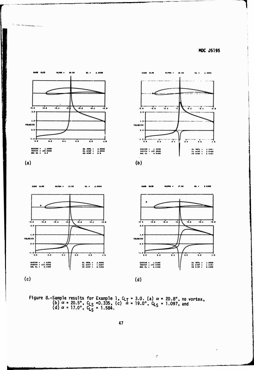
n

HOC J5195

•i • I.MM •KM • «« M II • I ••••

•<•!•• a I. MM tntttt • IM.MM Ml (L I t.i

(a)

ei im • i. MM ct <•» • I.MM M «I« • • •

»•mi • i itM mir«« ■ )•••••« Ml Cl • «IM

(b)

II ftlt • I «Ml Cl •■•> • t MM (• «IM t i nil

«inu ■ ii.M Cl • I.MM MMU • il.M

•MIM • I.MM rain» • III.MM Ml Cl ■ I.IIM

Cl »Tl I i.MM CL «lir • I.Ill« ct tiftr ■ i.iiM

UtlHI • I.IIM imr« ■ III.MM Ml CL ■ I.IIM

Cl Mil • I.MM Cl II« • I.«Ill Ct «IM • I.IIM

(c) (d)

Figure 8.-Sample results for Example 1. CLT = 3.0. (a) a » 20.8°, no vortex, jb) a = 20.5°. CLS =0.335. (c) a = 19.0°. CLC = 1.097, and (d)a = 17.0°, CL5 = 1.584. 5

47

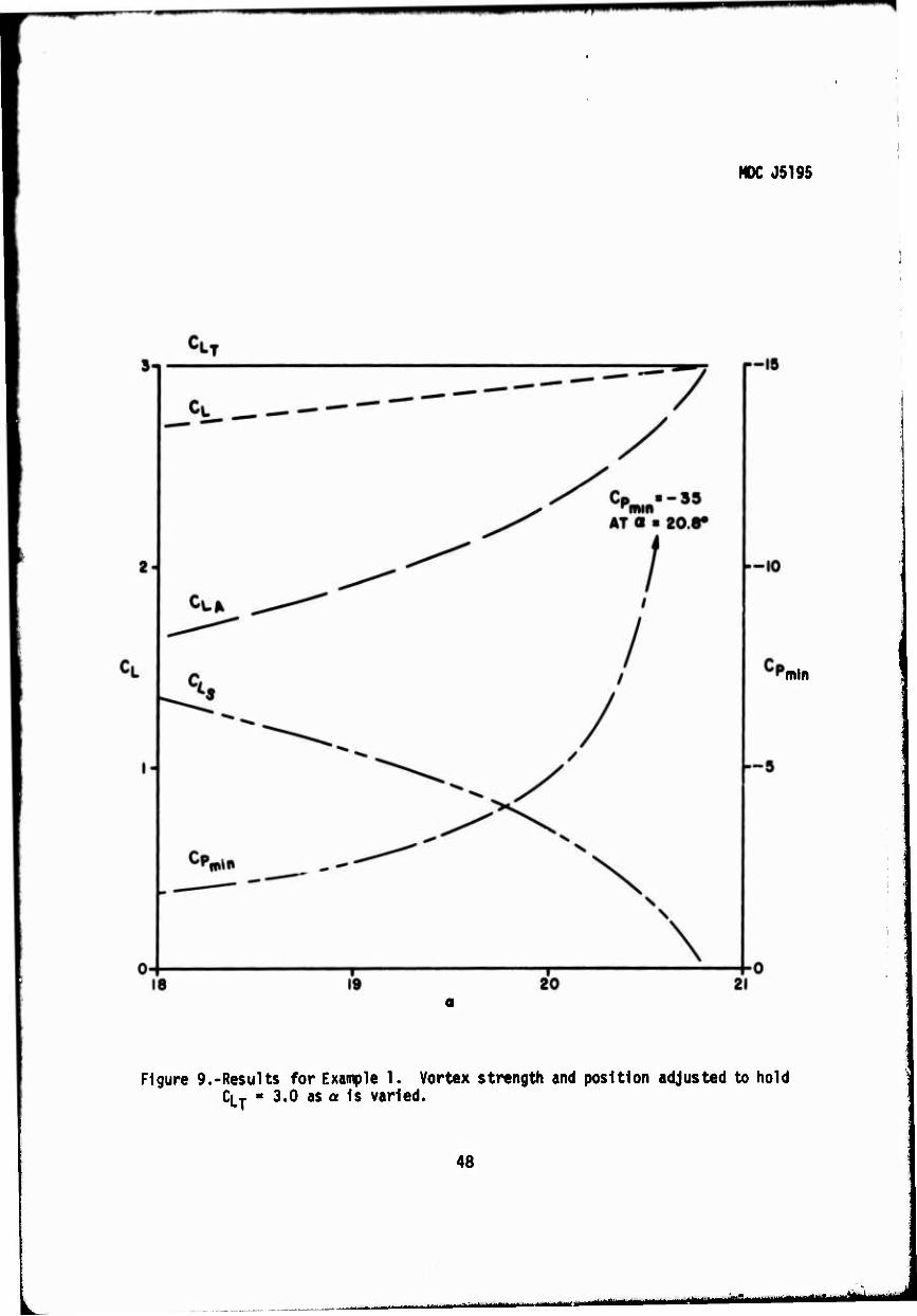
HOC J519S

min

Figure 9.-Results for Example 1. Vortex strength and position adjusted to hold CLT ■ 3.0 as a Is varied.

48

- — 1 ii m ■ «a

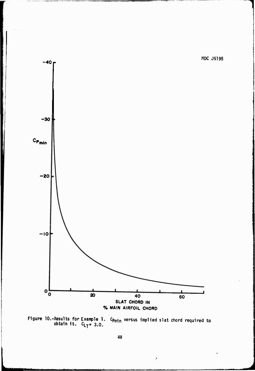
.^■^■..■■^. ..Willi.I MWIIIIIIIII^IUPH MW"1

-40

-30

Cp min

-20 -

-10 -

20 40 SLAT CHORD IN

% MAIN AIRFOIL CHORD

60

MDC J5195

Figure 10.-Results for Example 1. Cpmin versus Implied slat chord required to obtain It. CLT= 3.0.

49

\nt -' ' ■■ -■"—-■■■

.^-^IT—rim . ..ij, i iijMinniim.nHiinnni»ii !,.IIII)H IM um iiiiiiJiPnii^iipwiiiiN IIII i iiirii-gnnmnif'^"" j i ■■■»II u >--«'; i'"mw'

MDC J5195

«WM t |l.«• •I • I.IMI »tn* • i«. •• n a I.IIII

—^ ^ =—

•I .• ••.• ••.< •». b- •I.I •• .

^^--^^ ,

1 ^ «UM in J /

., .1- !

Mlllll • I.IIII rHITAV ■ III.IIII ML Cl • l.llll

n ton. • i.iin Ck «IIP a l.llll Cl IIII a I.IMI

•••■•• a l.llll »ITM a |II.UM III CL a l.llll

CL IITl a l.llll CL IIII a l.llll Cl IIII a l.llll

(a) (b)

tin» a u.ll Cl a I.lilt

Mlllll a l.llll »IM« a III.mi ML CL a l.llll

Cl IITl a l.lllt Cl «IIP a l.llll Cl «I» a I.till

(c)

Figure 11.-Sample results for Example 2. Vortex strength and position adjusted to hold Cpmin = -12 constant as a Is Increased.

(a) «= 15.0°. (b) a» 20.0°, and (c) a = 30.0°.

50

- ■■ kuataMBhautlii .-„■■....^■.■-^ ^ itaMi

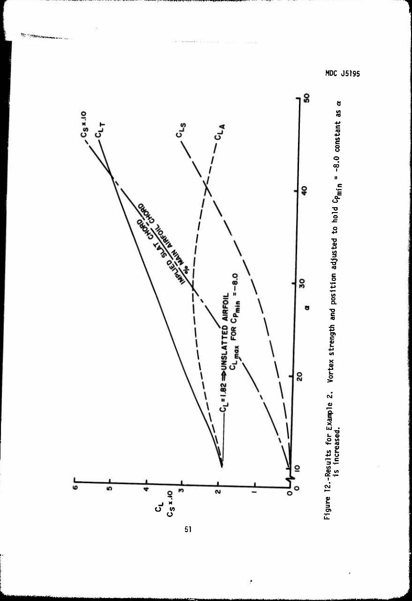
iMnn«*''''^"""1""""'"'""""""""1""''"

■'tormmmm

MDC J5195

ü w o

3

<a

c 8 o « oo

i

o •o o

B

I ■o c «

C t

■M

X

o

a> e—

X

i: « .o \n

t

CNJ

o>

51

k — - ■■ -

■ ^mam "wmpH^p '-■ l mmm^i^^mHmmmmm**'* ^r W^^^^&f™

MDC J5195

ö

58 c

</) c 8 o • CNJ ^-

II

c

J

o •M

■o

VI 3

o •r- •P

1 c «

I o

CM

!

i CO

Ü K

Ü

2 o>

52

- -■ - i - -- ^Mi^MM^M^MMMMk

MDC J5195

CLTs2.05(CpmJn = -l2, NO VORTEX)

CLT « 1-82 (Cpmjn s-8, NO VORTEX)

40 SLAT CHORD IN

% MAIN AIRFOIL CHORD

60

Figure 14.-Results for Example 2. Increase in CLT versus implied slat chord required to hold Cpmi-n = -8, and -12.

53

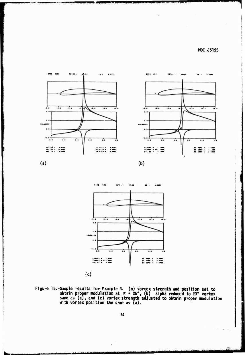
im^m**^^*?* -•—■»5-"W^^i^l^^ wmmm m^^m^^^^^m

MDC J5195

C4II Jltl «I.»«* • It •• CL ■ ■.«■•• CAtt Hit •(.»ft ■ tt.t* CL ■ l.tl»!

• •»IW1 ■ I.«tit TNITAV • II*.MM •It CL • t MM

CL T«TL • I.It«« CL «nr • •«IM ci mir • t-Mii

*«tiv« • i.«it« THITA* ■ nt.ttt» •IL CL ■ •.!«••

CL T«fL • ■.■l»l CL *i«r • •.nit C* «!■» ■ l.ltlf

(a) (b)

c«sa Mil *LM* ■ ll.lt CL • l.tlftl

lAtl«« ■ t.tltt THITAV • Itt.tttt ••L CL ■ tlltt

•b ratt • i.»itt CL mtr • t.iiit et ttiv • «.it«»

(c) i

Figure 15.-Sample results for Example 3. (a) vortex strength and position set to obtain proper modulation at a • 25°, (b) alpha reduced to 20° vortex same as (a), and (c) vortex strength adjusted to obtain proper modulation with vortex position the same as (a).

54

.t^MM^Ma^MHC^lMaMiaaiiMuilitfaMHikaiia tfl imt

(a)

MDC J5195

cat• 1au ALt•a • .. ... ...... CAll IIIU ....

-- --~--~----~----r----,----~·-----..... ·• .. "'·I\ ·• .. • t . I .... . ... . ...

• .• r------- -+-'t---Or-----------. · · ·+---------------------H-----------------~~~

. ..

... WtLec "'

•.• +---------o;:::-#--:;::oo--------t

~---:A( ..

·· · ·~------~--------r---~---r------~r-------~ ... ... IAtUI I . ttlt .... ,... ,,, ..... tilL. CL t , tttt

...

(c)

... A tiP .. I . till ...... ..... ,

...... . ...

(b)

.. ... ...... . .... . , ... ,... .. ..... . ~tL n .

. .. ......

--~----~----r-----~----~----,------..... • 1 . 1 • l . t • I , I • t . t ·~ . I • 1 . 1 ... ... r -...

.. . .. ... ... ... . .. llltl • t I . tUI CL 'l' tfL t . tttf

1'WI'f&W Ut . I ttl CL aUf t . '"' tfL CL • 1 . 1111 C l aUf • t 1 111

·• .. . ... I'::-If

. I(

... ...

•1.. . • .•

---. ..

OL llf&. Cl. aUP .,,,

. .. . ...

Figure 16.-Sample results for Example 3. Vortex position fixed at a =25°. Vortex strength adjusted to obtain proper modulation as a is reduced: (a) a= 10°, (b) a= 5°, and (c) a= 0°.

55

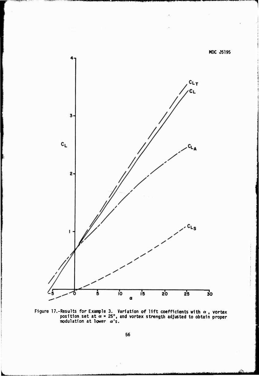
r^.I^r ^ li,J,m),mm9m^Aln}mmnr ji.,!!.! n^!, i ■ .■ Iliptjp^mp^^^^^^^yyill I P I !■ I ■ p I ^ I ■ ^ ■yva IL|

MDC J5195

30

Figure 17.-Results for Example 3. Variation of lift coefficients with a % vortex position set at a » 25°, and vortex strength adjusted to obtain proper modulation at lower a's.

56

- .._ ^^^.^^^^^.^t/t^j^tOt^m^

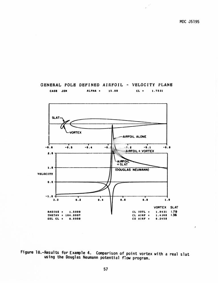
GENERAL POLE DEFINED AIRFOIL - VELOCITY PLANE CASI JSJI ALPHA : 15 . 00

SLAT

-1 . 1

1 . 1,-----------------------~~

VELOCITY

-a. 0 ~ . 0 0 . 1 1 . 4

UDIUS a 1.5001 TH£TAY • ...... ., C£L CL a 0. otOI

CL a a.nu

AIRFOIL ALONE

-0.1

••• 1 . 1 1.1

VORTEX SLAT CL TOTL • a.uu 1.79 CL """ • a.uu 1.36 CD AIIIF • o. zue

MDC J5195

Figure 18.-Results for Example 4. Comparison of point vortex with a real slat using the Douglas Neumann potential f~ow program.

57

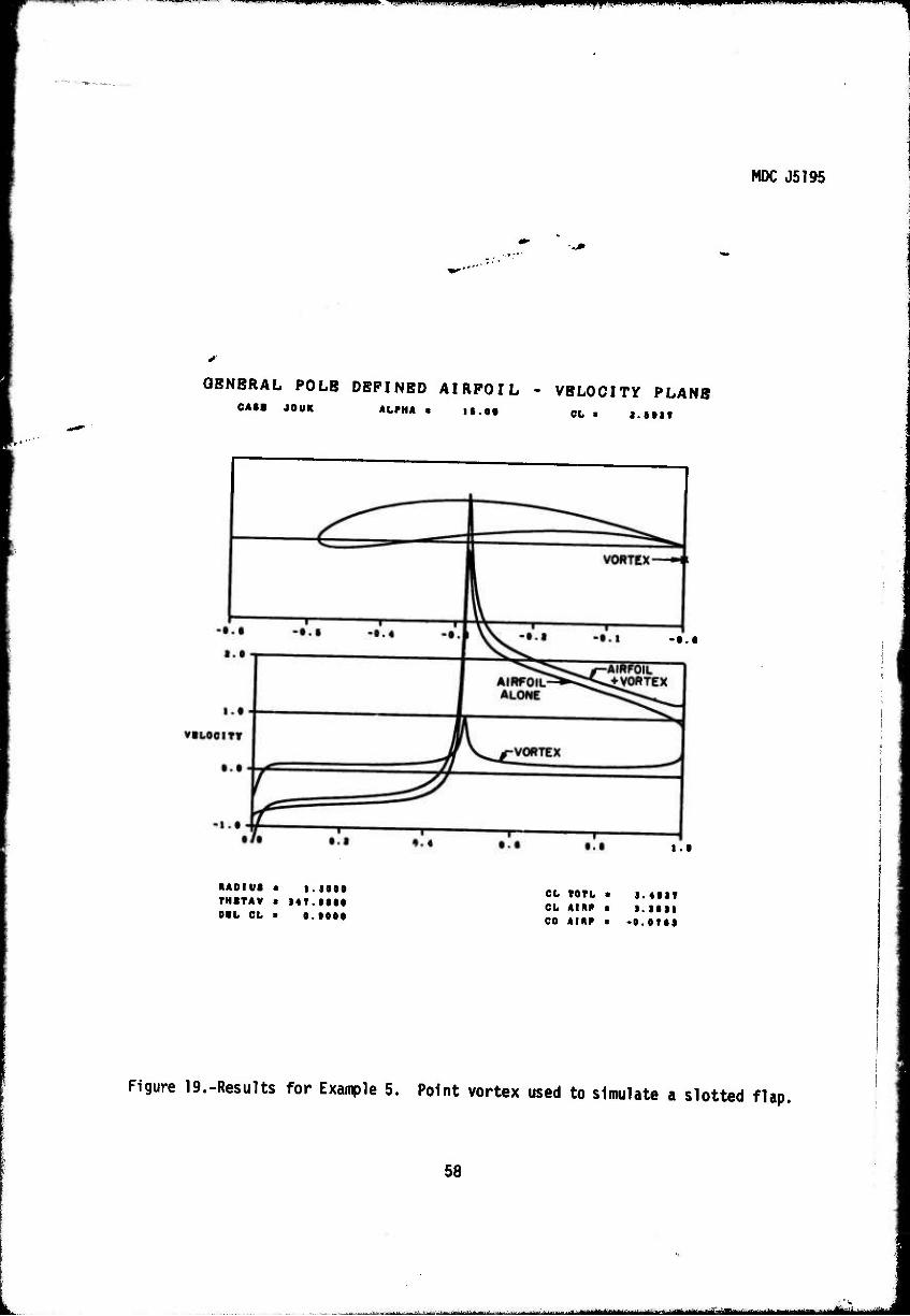
tmm l.lllll-l 1 ■■ W«HIHi^P^^pOT^WMPffP^H^^*^K9iWII|MIH IIBII1IIHIII

MOC J5195

GBNBRAL POLB DBPINBD AIRPOIL - VBLOCITY PLANS CAM JOUR ALPHA ■ |».e« CL > I.Stlf

RADIUS a I.1000 THITAV ■ 14T.I000 OIL CL « 0.1000

-0.0

1.0

CL TOTL a 1.400? CL AIRP a 1.1011 CD AIRP « .0.0T0I

Figure 19.-Results for Example 5. Point vortex used to simulate a slotted flap.

58

MIMMM MI 'H II*H1H —-"-"■■ MMMtta -^■^^;^^^^-^-^-^^-^^-^~ g^Jl^y—^^

MDC J5195

(a)

ELLIPSE-PLANE

(b) CIRCLE-PLANE

/ W^xj+lyj

\ MAIN FLOW \ STREAMLINES

-7777 •LOWER SURFACE T.E., Xj-^ -OB

UPPER SURFACE — T.E.,X3— +OD

*t'^ (c) HALF-PLANE 8 SLAT-CENTERED HALF-PLANE

(NOT TO SCALE)

Figure 20.-Domains used in the distributed singularity analysis; (a) ellipse- plane, (b) circle-plane, and (c) half-plane. (Reference 3).

59

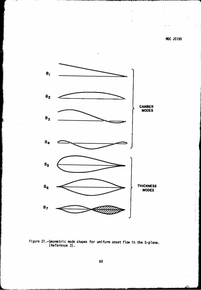
i >i MIHUIHI.» iua. i H> ■[•»(•voi^^mi mi . imiliiim.! .11 iiijiiiiVjfl ■» i i ■■...J». .. ••—

MDC J5195

B,

B2

B:

B,

» CAMBER MOOES

B.

B 6

B-

L THICKNESS MOOES

Figure 21.-Geometric mode shapes for uniform onset flow in the S-plane. (Reference 3).

60

. ~~. - mm —--*" -V Id

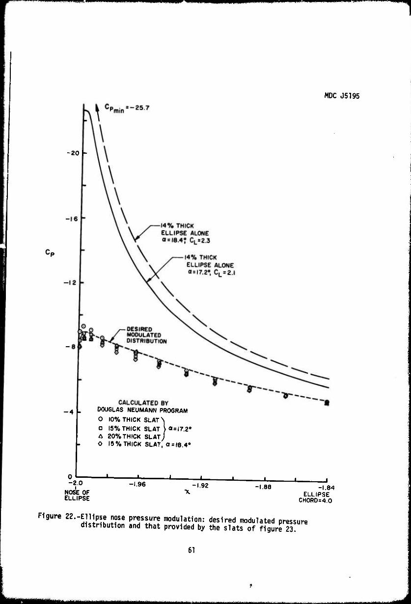
■— J1"1»11"1 HUI t»u <i .i. mit^w^^m^mmmmmmmur^mmmm mM^*mmmrm «KV > ■ ■ • in^U

MDC J5195

-20 h

-4h CALCULATED BY

DOUGLAS NEUMANN PROGRAM

0 10% THICK SLAT N Q 15% THICK SLAT iasl7.20

A 20%THICK SLATJ O 15% THICK SLAT, 0 = 18.4°

0 -2.0

NOSE OF ELLIPSE

J L J L -1.96 -1.92

J U -1.88 -1.84

ELLIPSE CH0RD=4.0

Figure 22.-Ellipse nose pressure modulation: desired modulated pressure distribution and that provided by the slats of figure 23.

61

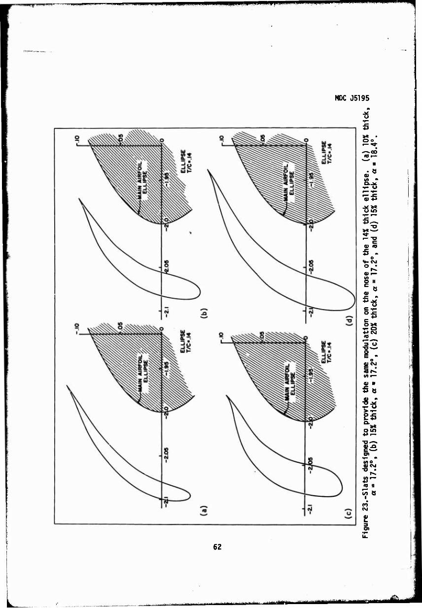
LLWilji J I 1 •-

MDC J5195

o

«I—

t- o

u in

«~

i— tJ c <u to 5 . 0^ OJi—

O II

«8

Ü

I*

-3 o

0) II

Se

15 o.

i^

« n

• CO CM

21 3

62

L^ mttatUM ■ tm mä -■ ■ ■■■■'■■' -