1 1 Slide © 2005 Thomson/South-Western Chapter 7, Part A Sampling and Sampling Distributions Sampling Distribution of Sampling Distribution of Introduction.

1 1 Slide

Slide

© 2005 Thomson/South-Western

Chapter 7, Part ASampling and Sampling Distributions

x Sampling Distribution of

Introduction to Sampling Distributions

Point Estimation

Simple Random Sampling

2 2 Slide

Slide


The purpose of statistical inference is to obtain information about a population from information contained in a sample.

The purpose of statistical inference is to obtain information about a population from information contained in a sample.

Statistical Inference

A population is the set of all the elements of interest. A population is the set of all the elements of interest.

A sample is a subset of the population. A sample is a subset of the population.

3 3 Slide

Slide


The sample results provide only estimates of the values of the population characteristics. The sample results provide only estimates of the values of the population characteristics.

A parameter is a numerical characteristic of a population. A parameter is a numerical characteristic of a population.

With proper sampling methods, the sample results can provide “good” estimates of the population characteristics.

With proper sampling methods, the sample results can provide “good” estimates of the population characteristics.

Statistical Inference

4 4 Slide

Slide


Simple Random Sampling:Finite Population

Finite populations are often defined by lists such as:• Organization membership roster• Credit card account numbers• Inventory product numbers A simple random sample of size n from a

finite population of size N is a sample selected such that each possible sample of size n has the same probability of being selected.

5 5 Slide

Slide


s is the point estimator of the population standard deviation . s is the point estimator of the population standard deviation .

In point estimation we use the data from the sample to compute a value of a sample statistic that serves as an estimate of a population parameter.

In point estimation we use the data from the sample to compute a value of a sample statistic that serves as an estimate of a population parameter.

Point Estimation

We refer to as the point estimator of the population mean . We refer to as the point estimator of the population mean .

x

is the point estimator of the population proportion p. is the point estimator of the population proportion p.p

6 6 Slide

Slide


Sampling Error

Statistical methods can be used to make probability statements about the size of the sampling error.

Sampling error is the result of using a subset of the population (the sample), and not the entire population.

The absolute value of the difference between an unbiased point estimate and the corresponding population parameter is called the sampling error.

When the expected value of a point estimator is equal to the population parameter, the point estimator is said to be unbiased.

7 7 Slide

Slide


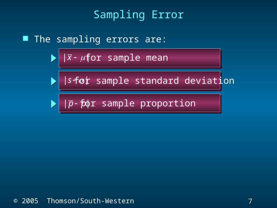
Sampling Error

The sampling errors are:

| |p p for sample proportion

| |s for sample standard deviation

| |x for sample mean

8 8 Slide

Slide


Example: St. Andrew’s

St. Andrew’s College receives900 applications annually fromprospective students. Theapplication form contains a variety of informationincluding the individual’sscholastic aptitude test (SAT) score and whether

or notthe individual desires on-campus housing.

9 9 Slide

Slide



The director of admissionswould like to know thefollowing information:• the average SAT score for the 900 applicants, and• the proportion of

applicants that want to live on campus.

10 10 Slide

Slide



We will now look at threealternatives for obtaining thedesired information. Conducting a census of the entire 900 applicants Selecting a sample of 30

applicants, using a random number table Selecting a sample of 30 applicants, using

Excel

11 11 Slide

Slide


Conducting a Census

If the relevant data for the entire 900 applicants were in the college’s database, the population parameters of interest could be calculated using the formulas presented in Chapter 3.

We will assume for the moment that conducting a census is practical in this example.

12 12 Slide

Slide


990900

ix

2( )80

900ix

Conducting a Census

648.72

900p

Population Mean SAT Score

Population Standard Deviation for SAT Score

Population Proportion Wanting On-Campus Housing

13 13 Slide

Slide


as Point Estimator of x

as Point Estimator of pp

29,910997

30 30ix

x

2( ) 163,99675.2

29 29ix x

s

20 30 .68p

Point Estimation

Note: Different random numbers would haveidentified a different sample which would haveresulted in different point estimates.

s as Point Estimator of

14 14 Slide

Slide


PopulationParameter

PointEstimator

PointEstimate

ParameterValue

m = Population mean SAT score

990 997

s = Population std. deviation for SAT score

80 s = Sample std. deviation for SAT score

75.2

p = Population proportion wanting campus housing

.72 .68

Summary of Point EstimatesObtained from a Simple Random Sample

= Sample mean SAT score x

= Sample proportion wanting campus housing

p

15 15 Slide

Slide


Process of Statistical Inference

The value of is used tomake inferences about

the value of m.

x The sample data provide a value for

the sample mean .x

A simple random sampleof n elements is selected

from the population.

Population with mean

m = ?

Sampling Distribution of x

16 16 Slide

Slide


The sampling distribution of is the probabilitydistribution of all possible values of the sample mean .

x

x


where: = the population mean

E( ) = x

xExpected Value of

17 17 Slide

Slide



Finite Population Infinite Population

x n

N nN

( )1

x n

• is referred to as the standard error of the

mean.

x

• A finite population is treated as being infinite if n/N < .05.

• is the finite correction factor.( ) / ( )N n N 1

xStandard Deviation of

18 18 Slide

Slide


Form of the Sampling Distribution of x

If we use a large (n > 30) simple random sample, thecentral limit theorem enables us to conclude that thesampling distribution of can be approximated bya normal distribution.

x

When the simple random sample is small (n < 30),the sampling distribution of can be considerednormal only if we assume the population has anormal distribution.

x

19 19 Slide

Slide


8014.6

30x

n

( ) 990E x x

Sampling Distribution of for SAT Scoresx

SamplingDistribution

of x

20 20 Slide

Slide


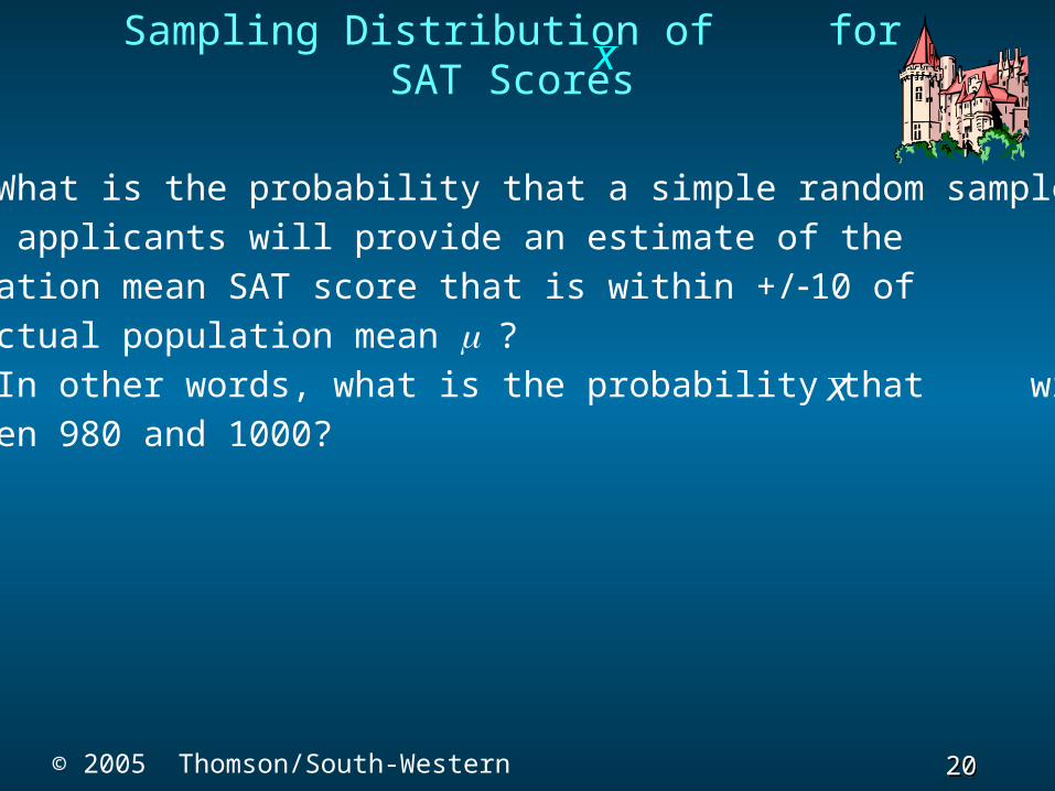
What is the probability that a simple random sampleof 30 applicants will provide an estimate of thepopulation mean SAT score that is within +/-10 ofthe actual population mean ? In other words, what is the probability that will bebetween 980 and 1000?

x


21 21 Slide

Slide


Step 1: Calculate the z-value at the upper endpoint of the interval.

z = (1000 - 990)/14.6= .68

P(z < .68) = .7517

Step 2: Find the area under the curve to the left of the upper endpoint.


22 22 Slide

Slide



Cumulative Probabilities for the Standard Normal

Distributionz .00 .01 .02 .03 .04 .05 .06 .07 .08 .09

. . . . . . . . . . .

.5 .6915 .6950 .6985 .7019 .7054 .7088 .7123 .7157 .7190 .7224

.6 .7257 .7291 .7324 .7357 .7389 .7422 .7454 .7486 .7517 .7549

.7 .7580 .7611 .7642 .7673 .7704 .7734 .7764 .7794 .7823 .7852

.8 .7881 .7910 .7939 .7967 .7995 .8023 .8051 .8078 .8106 .8133

.9 .8159 .8186 .8212 .8238 .8264 .8289 .8315 .8340 .8365 .8389

. . . . . . . . . . .

23 23 Slide

Slide



x990


of x14.6x

1000

Area = .7517

24 24 Slide

Slide


Step 3: Calculate the z-value at the lower endpoint of the interval.

Step 4: Find the area under the curve to the left of the lower endpoint.

z = (980 - 990)/14.6= - .68

P(z < -.68) = P(z > .68)

= .2483= 1 - . 7517

= 1 - P(z < .68)


25 25 Slide

Slide



x980 990

Area = .2483


of x14.6x

26 26 Slide

Slide



Step 5: Calculate the area under the curve between the lower and upper endpoints of the interval.

P(-.68 < z < .68) = P(z < .68) - P(z < -.68)= .7517 - .2483= .5034

The probability that the sample mean SAT score willbe between 980 and 1000 is:

P(980 < < 1000) = .5034x

27 27 Slide

Slide


x1000980 990


Area = .5034


of x14.6x

28 28 Slide

Slide


Relationship Between the Sample Size and the Sampling Distribution of x

Suppose we select a simple random sample of 100 applicants instead of the 30 originally considered.

E( ) = m regardless of the sample size. In our

example, E( ) remains at 990.

xx

Whenever the sample size is increased, the standard error of the mean is decreased. With the increase in the sample size to n = 100, the standard error of the mean is decreased to:

x

808.0

100x

n

29 29 Slide

Slide



( ) 990E x x

14.6x With n = 30,

8x With n = 100,

30 30 Slide

Slide


Recall that when n = 30, P(980 < < 1000) = .5034.x


We follow the same steps to solve for P(980 < < 1000) when n = 100 as we showed earlier when n = 30.

x

Now, with n = 100, P(980 < < 1000) = .7888.x Because the sampling distribution with n = 100 has a smaller standard error, the values of have less variability and tend to be closer to the population mean than the values of with n = 30.

x

x

31 31 Slide

Slide



x1000980 990

Area = .7888


of x8x

1 1 Slide © 2005 Thomson/South-Western Chapter 7, Part A Sampling and Sampling Distributions Sampling Distribution of Sampling Distribution of Introduction.

Documents

point estimator

sample mean

sample proportion

different sample

census population

entire population

sample standard deviation

sample statistic