1 © 2005 Thomson/South-Western © 2005 Thomson/South-Western Chapter 12 Chapter 12 Tests of Goodness of Fit and Tests of Goodness of Fit and Independence Independence Goodness of Fit Test: A Multinomial Population Goodness of Fit Test: A Multinomial Population Goodness of Fit Test: Poisson Goodness of Fit Test: Poisson and Normal Distributions and Normal Distributions Test of Independence Test of Independence

Welcome message from author
This document is posted to help you gain knowledge. Please leave a comment to let me know what you think about it! Share it to your friends and learn new things together.
Transcript
1 1 Slide
Slide
© 2005 Thomson/South-Western© 2005 Thomson/South-Western
Chapter 12Chapter 12 Tests of Goodness of Fit and Tests of Goodness of Fit and
IndependenceIndependence Goodness of Fit Test: A Multinomial Population Goodness of Fit Test: A Multinomial Population
Goodness of Fit Test: PoissonGoodness of Fit Test: Poisson and Normal Distributionsand Normal Distributions
Test of IndependenceTest of Independence
2 2 Slide
Slide
© 2005 Thomson/South-Western© 2005 Thomson/South-Western
Hypothesis (Goodness of Fit) TestHypothesis (Goodness of Fit) Testfor Proportions of a Multinomial for Proportions of a Multinomial
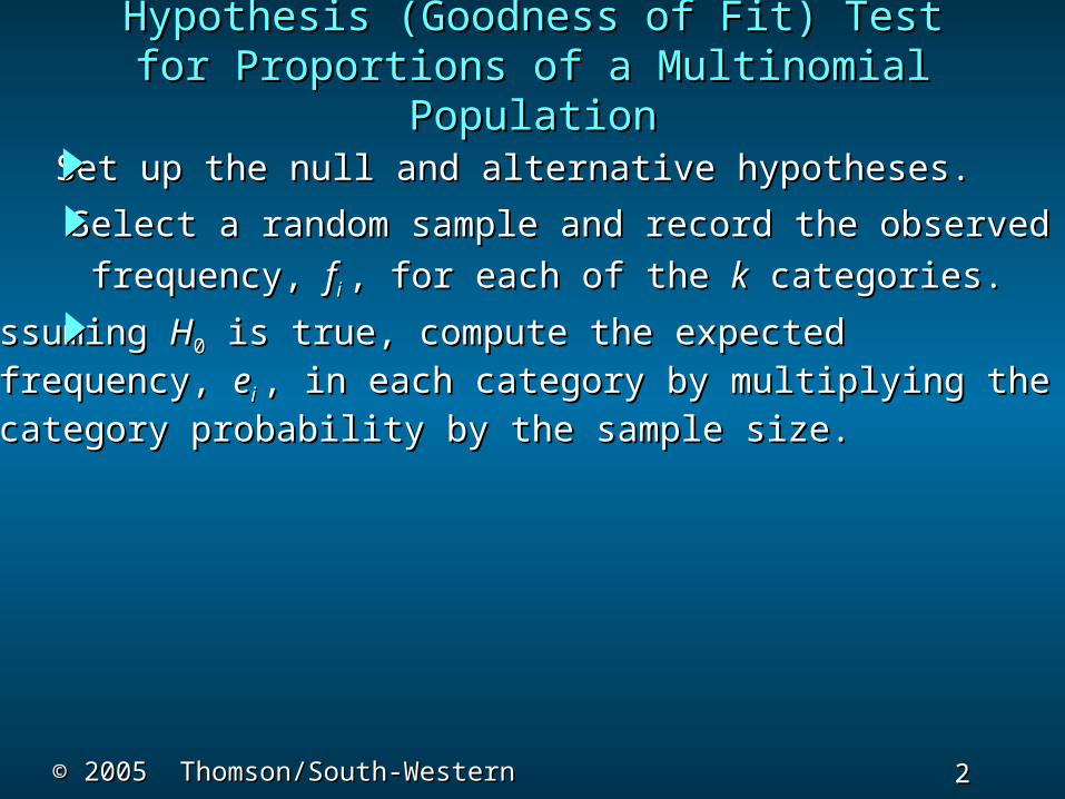
PopulationPopulation1.1. Set up the null and alternative hypotheses. Set up the null and alternative hypotheses.
2.2. Select a random sample and record the observed Select a random sample and record the observed
frequency, frequency, ffi i , for each of the , for each of the kk categories. categories.
3.3. Assuming Assuming HH00 is true, compute the expected is true, compute the expected frequency, frequency, eei i , in each category by multiplying the, in each category by multiplying the category probability by the sample size.category probability by the sample size.
3 3 Slide
Slide
© 2005 Thomson/South-Western© 2005 Thomson/South-Western
Hypothesis (Goodness of Fit) TestHypothesis (Goodness of Fit) Testfor Proportions of a Multinomial for Proportions of a Multinomial
PopulationPopulation
22
1
( )f ee
i i
ii
k2
2
1
( )f ee
i i
ii
k
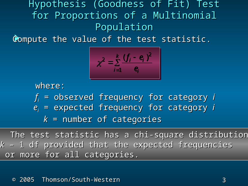
4.4. Compute the value of the test statistic. Compute the value of the test statistic.
Note: The test statistic has a chi-square distributionNote: The test statistic has a chi-square distributionwith with kk – 1 df provided that the expected frequencies – 1 df provided that the expected frequenciesare 5 or more for all categories.are 5 or more for all categories.
ffii = observed frequency for category = observed frequency for category iieeii = expected frequency for category = expected frequency for category ii
kk = number of categories = number of categories
where:where:
4 4 Slide
Slide
© 2005 Thomson/South-Western© 2005 Thomson/South-Western
Hypothesis (Goodness of Fit) TestHypothesis (Goodness of Fit) Testfor Proportions of a Multinomial for Proportions of a Multinomial
PopulationPopulation
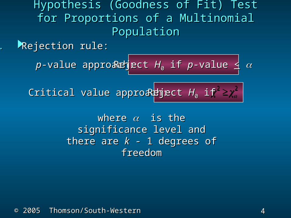
where where is the significance is the significance level andlevel and
there are there are kk - 1 degrees of - 1 degrees of freedomfreedom
pp-value approach:-value approach:
Critical value approach:Critical value approach:
Reject Reject HH00 if if pp-value -value <<
5.5. Rejection rule: Rejection rule:
2 2 2 2 Reject Reject HH00 if if
5 5 Slide
Slide
© 2005 Thomson/South-Western© 2005 Thomson/South-Western
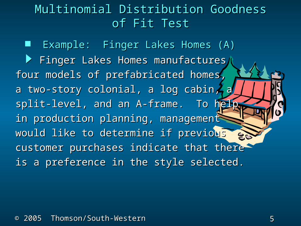
Multinomial Distribution Goodness of Fit Multinomial Distribution Goodness of Fit TestTest
Example: Finger Lakes Homes (A)Example: Finger Lakes Homes (A)
Finger Lakes Homes manufacturesFinger Lakes Homes manufactures
four models of prefabricated homes,four models of prefabricated homes,
a two-story colonial, a log cabin, aa two-story colonial, a log cabin, a
split-level, and an A-frame. To helpsplit-level, and an A-frame. To help
in production planning, managementin production planning, management
would like to determine if previous would like to determine if previous
customer purchases indicate that therecustomer purchases indicate that there
is a preference in the style selected.is a preference in the style selected.
6 6 Slide
Slide
© 2005 Thomson/South-Western© 2005 Thomson/South-Western
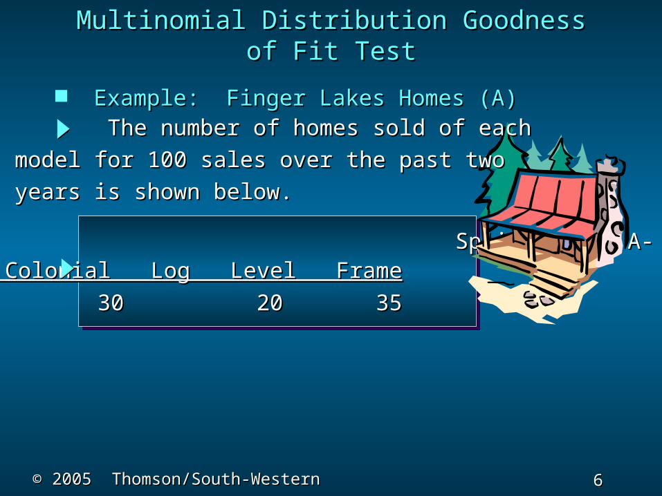
Split- A-Split- A-Model Colonial Log Level FrameModel Colonial Log Level Frame
# Sold# Sold 30 20 35 15 30 20 35 15
The number of homes sold of eachThe number of homes sold of each
model for 100 sales over the past twomodel for 100 sales over the past two
years is shown below.years is shown below.
Multinomial Distribution Goodness of Fit Multinomial Distribution Goodness of Fit TestTest
Example: Finger Lakes Homes (A)Example: Finger Lakes Homes (A)
7 7 Slide
Slide
© 2005 Thomson/South-Western© 2005 Thomson/South-Western
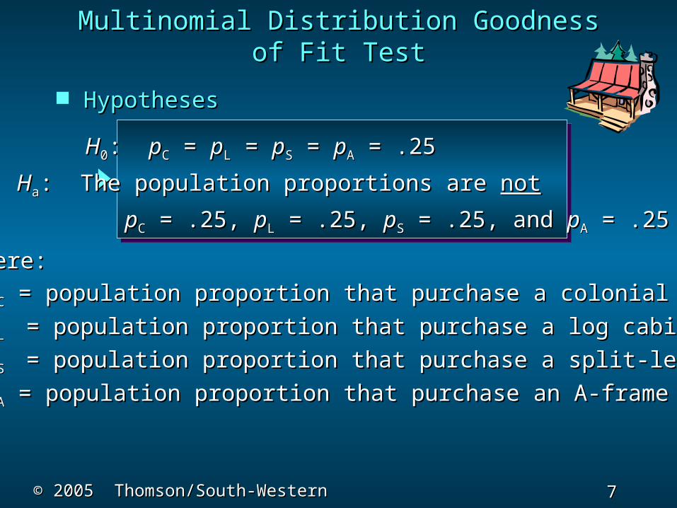
HypothesesHypotheses
Multinomial Distribution Goodness of Fit Multinomial Distribution Goodness of Fit TestTest
where:where:
ppCC = population proportion that purchase a colonial = population proportion that purchase a colonial
ppL L = population proportion that purchase a log cabin = population proportion that purchase a log cabin
ppS S = population proportion that purchase a split-level = population proportion that purchase a split-level
ppAA = population proportion that purchase an A-frame = population proportion that purchase an A-frame
HH00: : ppCC = = ppLL = = ppSS = = ppAA = .25 = .25
HHaa: The population proportions are : The population proportions are notnot
ppCC = .25, = .25, ppLL = .25, = .25, ppSS = .25, and = .25, and ppAA = .25 = .25

8 8 Slide
Slide
© 2005 Thomson/South-Western© 2005 Thomson/South-Western
Rejection RuleRejection Rule
22
7.815 7.815
Do Not Reject H0Do Not Reject H0 Reject H0Reject H0
Multinomial Distribution Goodness of Fit Multinomial Distribution Goodness of Fit TestTest
With With = .05 and = .05 and
kk - 1 = 4 - 1 = 3 - 1 = 4 - 1 = 3
degrees of freedomdegrees of freedom
Reject H0 if if pp-value -value << .05 or .05 or 22 > 7.815. > 7.815.
9 9 Slide
Slide
© 2005 Thomson/South-Western© 2005 Thomson/South-Western
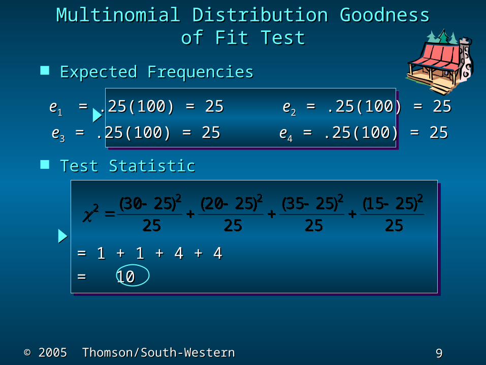
Expected FrequenciesExpected Frequencies
Test StatisticTest Statistic
22 2 2 230 25
2520 25
2535 25
2515 25
25
( ) ( ) ( ) ( )22 2 2 230 25
2520 25
2535 25
2515 25
25
( ) ( ) ( ) ( )
Multinomial Distribution Goodness of Fit Multinomial Distribution Goodness of Fit TestTest
ee1 1 = .25(100) = 25 = .25(100) = 25 ee22 = .25(100) = 25 = .25(100) = 25
ee33 = .25(100) = 25 = .25(100) = 25 ee44 = .25(100) = 25 = .25(100) = 25
= 1 + 1 + 4 + 4 = 1 + 1 + 4 + 4
= 10= 10
10 10 Slide
Slide
© 2005 Thomson/South-Western© 2005 Thomson/South-Western
Multinomial Distribution Goodness of Fit Multinomial Distribution Goodness of Fit TestTest
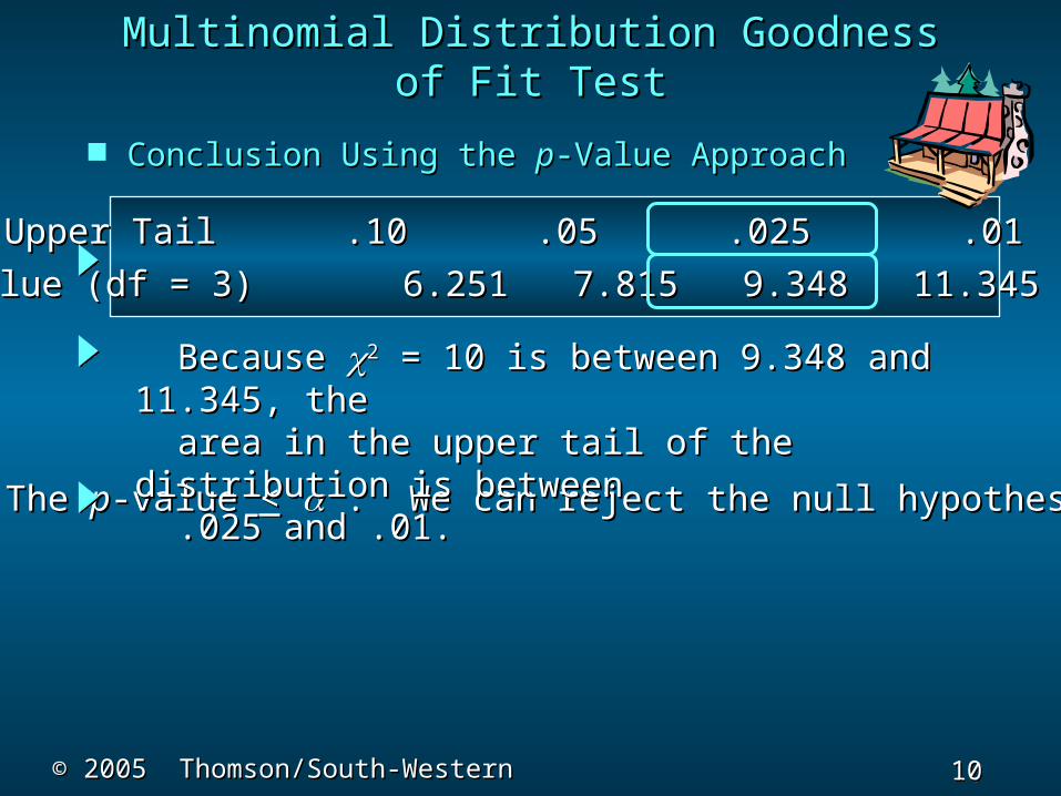
Conclusion Using the Conclusion Using the pp-Value Approach-Value Approach
The The pp-value -value << . We can reject the null hypothesis. . We can reject the null hypothesis.
Because Because 22 = 10 is between 9.348 and 11.345, = 10 is between 9.348 and 11.345, thethe area in the upper tail of the distribution is area in the upper tail of the distribution is betweenbetween .025 and .01..025 and .01.
Area in Upper Tail .10 .05 .025 .01 .005Area in Upper Tail .10 .05 .025 .01 .005
22 Value (df = 3) 6.251 7.815 9.348 11.345 12.838 Value (df = 3) 6.251 7.815 9.348 11.345 12.838
11 11 Slide
Slide
© 2005 Thomson/South-Western© 2005 Thomson/South-Western
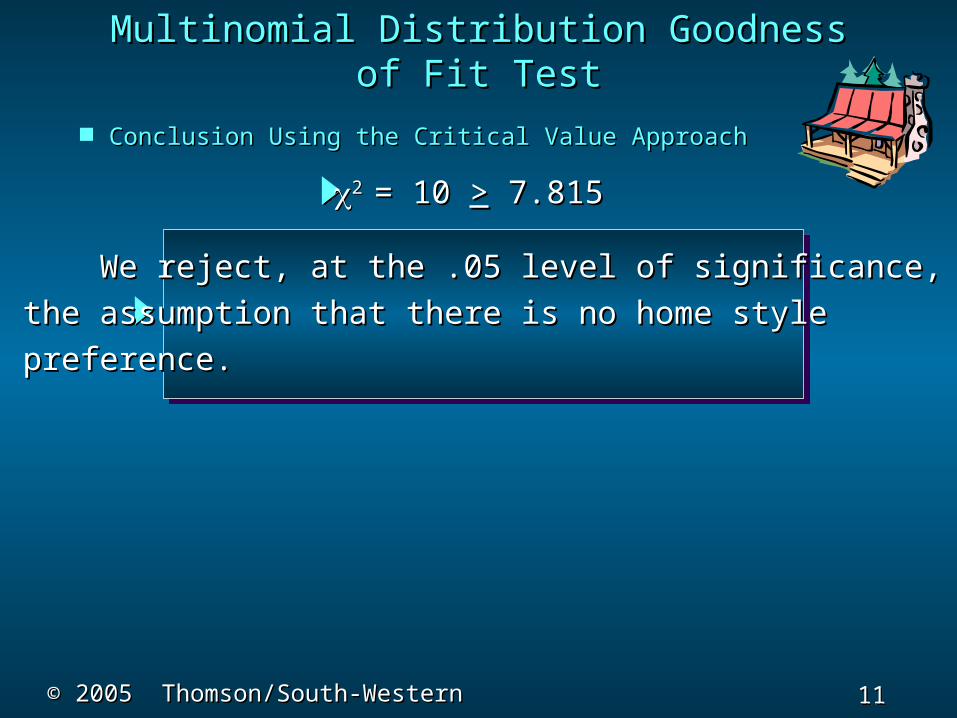
Conclusion Using the Critical Value ApproachConclusion Using the Critical Value Approach
Multinomial Distribution Goodness of Fit Multinomial Distribution Goodness of Fit TestTest
We reject, at the .05 level of significance,We reject, at the .05 level of significance,
the assumption that there is no home stylethe assumption that there is no home style
preference.preference.
2 2 = 10 = 10 >> 7.815 7.815
12 12 Slide
Slide
© 2005 Thomson/South-Western© 2005 Thomson/South-Western
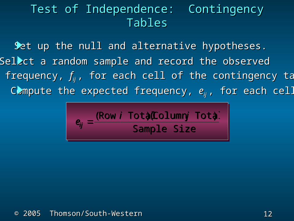
Test of Independence: Contingency Test of Independence: Contingency TablesTables
ei j
ij (Row Total )(Column Total )
Sample Sizee
i jij
(Row Total )(Column Total ) Sample Size
1.1. Set up the null and alternative hypotheses. Set up the null and alternative hypotheses.
2.2. Select a random sample and record the observed Select a random sample and record the observed
frequency, frequency, ffij ij , for each cell of the contingency table., for each cell of the contingency table.
3.3. Compute the expected frequency, Compute the expected frequency, eeij ij , for each cell., for each cell.
13 13 Slide
Slide
© 2005 Thomson/South-Western© 2005 Thomson/South-Western
Test of Independence: Contingency Test of Independence: Contingency TablesTables
22
( )f e
eij ij
ijji2
2
( )f e
eij ij
ijji
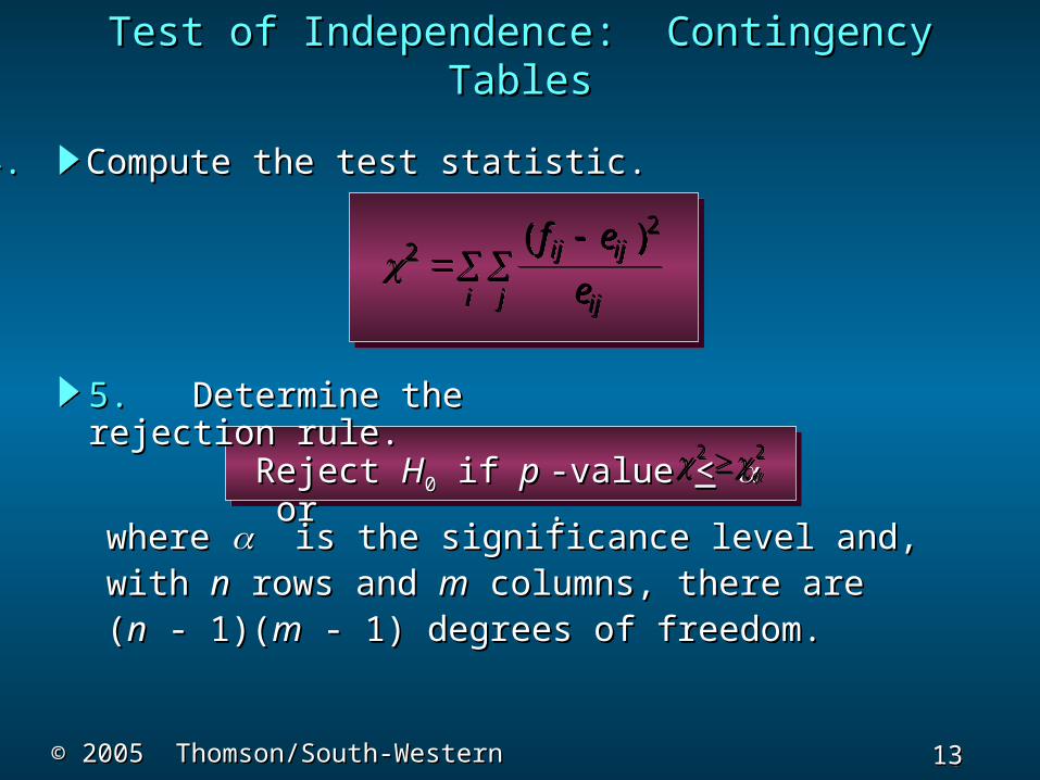
5.5. Determine the rejection rule. Determine the rejection rule.
Reject Reject HH00 if if p p -value -value << or or . .
2 2 2 2
4.4. Compute the test statistic. Compute the test statistic.
where where is the significance level and, is the significance level and,with with nn rows and rows and mm columns, there are columns, there are((nn - 1)( - 1)(mm - 1) degrees of freedom. - 1) degrees of freedom.

14 14 Slide
Slide
© 2005 Thomson/South-Western© 2005 Thomson/South-Western
Each home sold by Finger LakesEach home sold by Finger Lakes
Homes can be classified according toHomes can be classified according to
price and to style. Finger Lakes’price and to style. Finger Lakes’
manager would like to determine ifmanager would like to determine if
the price of the home and the style ofthe price of the home and the style of
the home are independent variables.the home are independent variables.
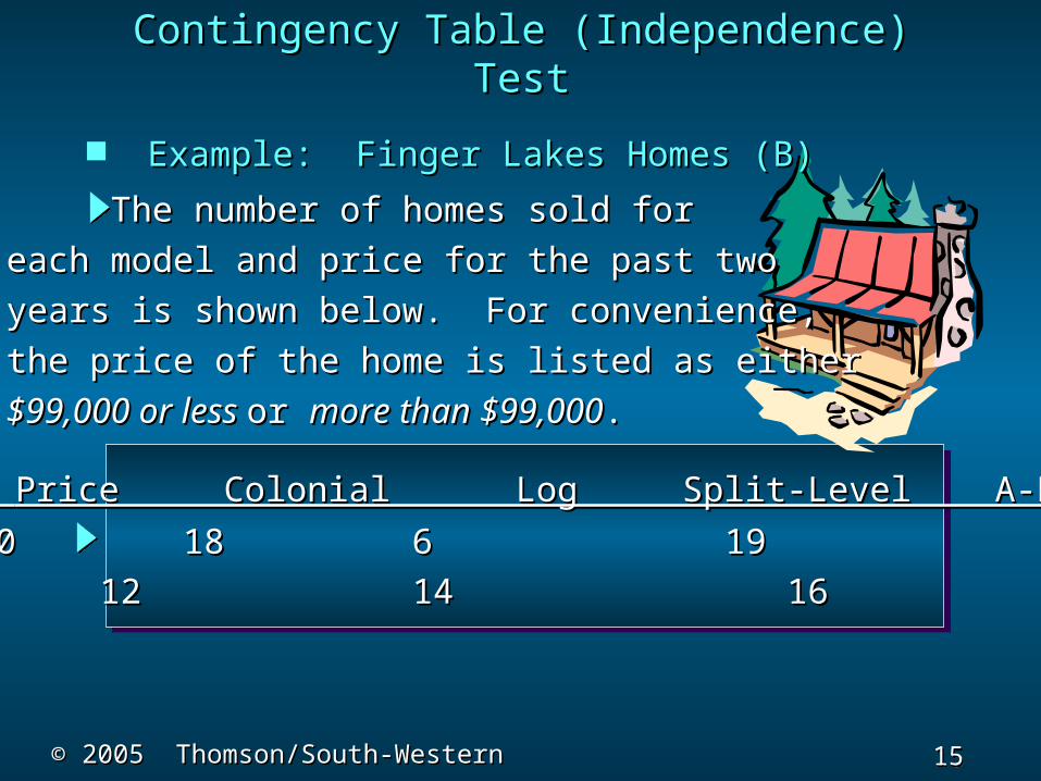
Contingency Table (Independence) TestContingency Table (Independence) Test
Example: Finger Lakes Homes (B)Example: Finger Lakes Homes (B)
15 15 Slide
Slide
© 2005 Thomson/South-Western© 2005 Thomson/South-Western
Price Colonial Log Split-Level A-FramePrice Colonial Log Split-Level A-Frame
The number of homes sold forThe number of homes sold for
each model and price for the past twoeach model and price for the past two
years is shown below. For convenience,years is shown below. For convenience,
the price of the home is listed as eitherthe price of the home is listed as either
$99,000 or less $99,000 or less or or more than $99,000more than $99,000..
> $99,000 12 14 > $99,000 12 14 16 316 3<< $99,000 18 $99,000 18 6 19 12 6 19 12
Contingency Table (Independence) TestContingency Table (Independence) Test
Example: Finger Lakes Homes (B)Example: Finger Lakes Homes (B)
16 16 Slide
Slide
© 2005 Thomson/South-Western© 2005 Thomson/South-Western
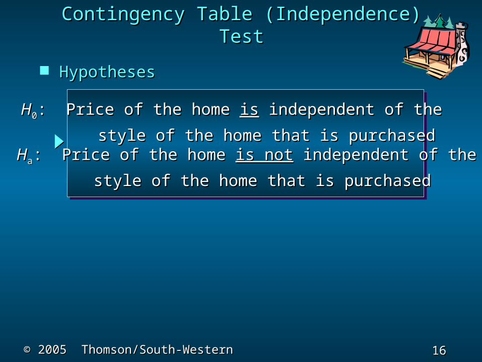
HypothesesHypotheses
Contingency Table (Independence) TestContingency Table (Independence) Test
HH00: Price of the home : Price of the home isis independent of the independent of the
style of the home that is purchasedstyle of the home that is purchasedHHaa: Price of the home : Price of the home is notis not independent of the independent of the
style of the home that is purchasedstyle of the home that is purchased
17 17 Slide
Slide
© 2005 Thomson/South-Western© 2005 Thomson/South-Western
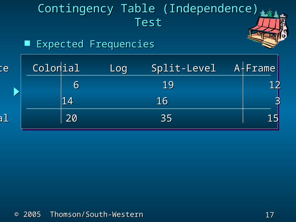
Expected FrequenciesExpected Frequencies
Contingency Table (Independence) TestContingency Table (Independence) Test
PricePrice Colonial Log Split-Level A-Frame Total Colonial Log Split-Level A-Frame Total
<< $99K $99K
> $99K> $99K
TotalTotal 30 20 35 15 10030 20 35 15 100
12 12 14 16 3 45 14 16 3 45
18 6 19 12 5518 6 19 12 55
18 18 Slide
Slide
© 2005 Thomson/South-Western© 2005 Thomson/South-Western
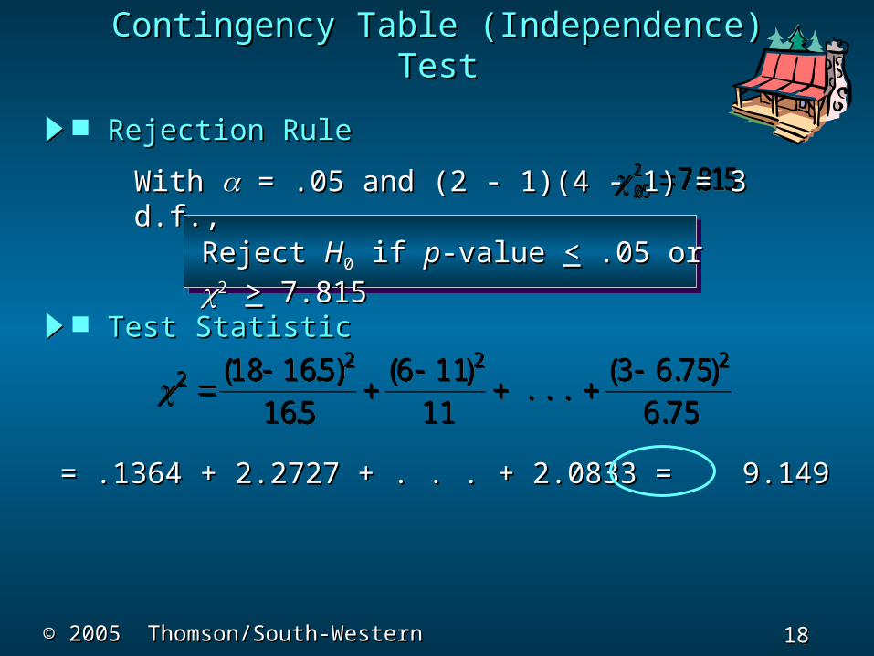
Rejection RuleRejection Rule
Contingency Table (Independence) TestContingency Table (Independence) Test
2.05 7.815 2.05 7.815 With With = .05 and (2 - 1)(4 - 1) = 3 d.f., = .05 and (2 - 1)(4 - 1) = 3 d.f.,
Reject Reject HH00 if if pp-value -value << .05 or .05 or 22 >> 7.8157.815
22 2 218 16 5
16 56 11
113 6 75
6 75 ( . )
.( )
. .( . )
. . 2
2 2 218 16 516 5
6 1111
3 6 756 75
( . ).
( ). .
( . ).
.
= .1364 + 2.2727 + . . . + 2.0833 = 9.149= .1364 + 2.2727 + . . . + 2.0833 = 9.149
Test StatisticTest Statistic

19 19 Slide
Slide
© 2005 Thomson/South-Western© 2005 Thomson/South-Western
Conclusion Using the Conclusion Using the pp-Value Approach-Value Approach
The The pp-value -value << . We can reject the null hypothesis. . We can reject the null hypothesis.
Because Because 22 = 9.145 is between 7.815 and = 9.145 is between 7.815 and 9.348, the9.348, the area in the upper tail of the distribution is area in the upper tail of the distribution is betweenbetween .05 and .025..05 and .025.
Area in Upper Tail .10 .05 .025 .01 .005Area in Upper Tail .10 .05 .025 .01 .005
22 Value (df = 3) 6.251 7.815 9.348 11.345 12.838 Value (df = 3) 6.251 7.815 9.348 11.345 12.838
Contingency Table (Independence) TestContingency Table (Independence) Test

20 20 Slide
Slide
© 2005 Thomson/South-Western© 2005 Thomson/South-Western
Conclusion Using the Critical Value ApproachConclusion Using the Critical Value Approach
Contingency Table (Independence) TestContingency Table (Independence) Test
We reject, at the .05 level of We reject, at the .05 level of significance,significance,the assumption that the price of the the assumption that the price of the home ishome isindependent of the style of home that independent of the style of home that isispurchased.purchased.
2 2 = 9.145 = 9.145 >> 7.815 7.815

21 21 Slide
Slide
© 2005 Thomson/South-Western© 2005 Thomson/South-Western
Goodness of Fit Test: Poisson DistributionGoodness of Fit Test: Poisson Distribution
1.1. Set up the null and alternative hypotheses. Set up the null and alternative hypotheses.
HH00: Population has a Poisson probability distribution: Population has a Poisson probability distribution
HHaa: Population does not have a Poisson distribution: Population does not have a Poisson distribution
3.3. Compute the expected frequency of occurrences Compute the expected frequency of occurrences eeii for each value of the Poisson random variable.for each value of the Poisson random variable.
2.2. Select a random sample and Select a random sample and
a.a. Record the observed frequency Record the observed frequency ffii for each value of for each value of
the Poisson random variable.the Poisson random variable.
b.b. Compute the mean number of occurrences Compute the mean number of occurrences ..
22 22 Slide
Slide
© 2005 Thomson/South-Western© 2005 Thomson/South-Western
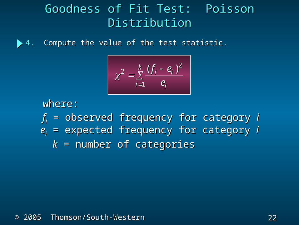
Goodness of Fit Test: Poisson DistributionGoodness of Fit Test: Poisson Distribution
22
1
( )f ee
i i
ii
k2
2
1
( )f ee
i i
ii
k
4.4. Compute the value of the test statistic. Compute the value of the test statistic.
ffii = observed frequency for category = observed frequency for category iieeii = expected frequency for category = expected frequency for category ii
kk = number of categories = number of categories
where:where:
23 23 Slide
Slide
© 2005 Thomson/South-Western© 2005 Thomson/South-Western
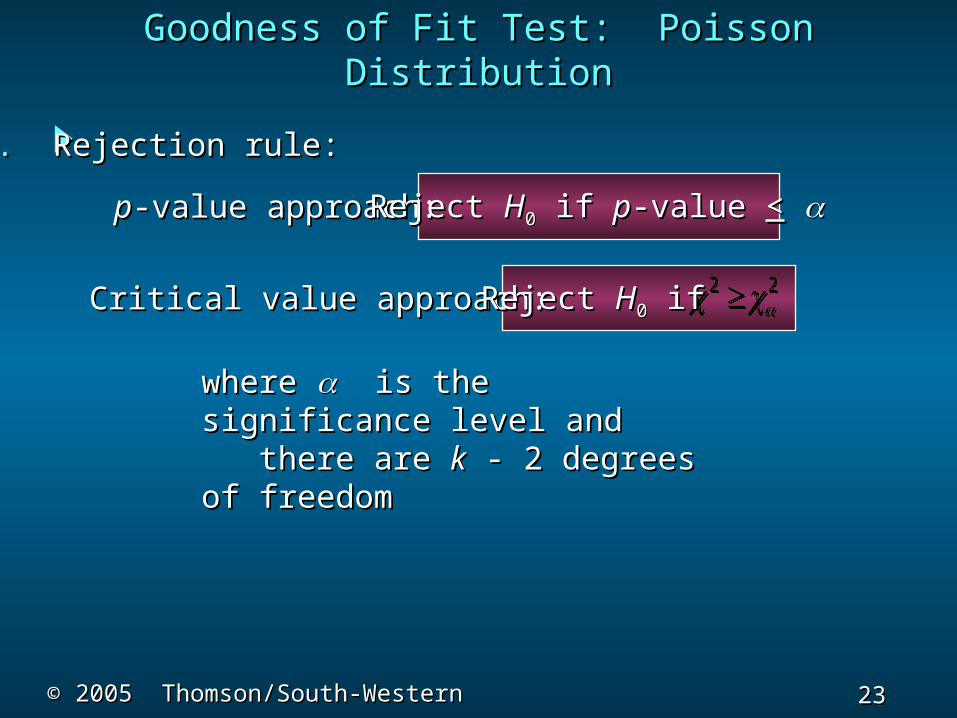
where where is the significance is the significance level andlevel and there are there are kk - 2 degrees of - 2 degrees of freedomfreedom
pp-value approach:-value approach:
Critical value approach:Critical value approach:
Reject Reject HH00 if if pp-value -value <<
5.5. Rejection rule: Rejection rule:
2 2 2 2 Reject Reject HH00 if if
Goodness of Fit Test: Poisson DistributionGoodness of Fit Test: Poisson Distribution
24 24 Slide
Slide
© 2005 Thomson/South-Western© 2005 Thomson/South-Western
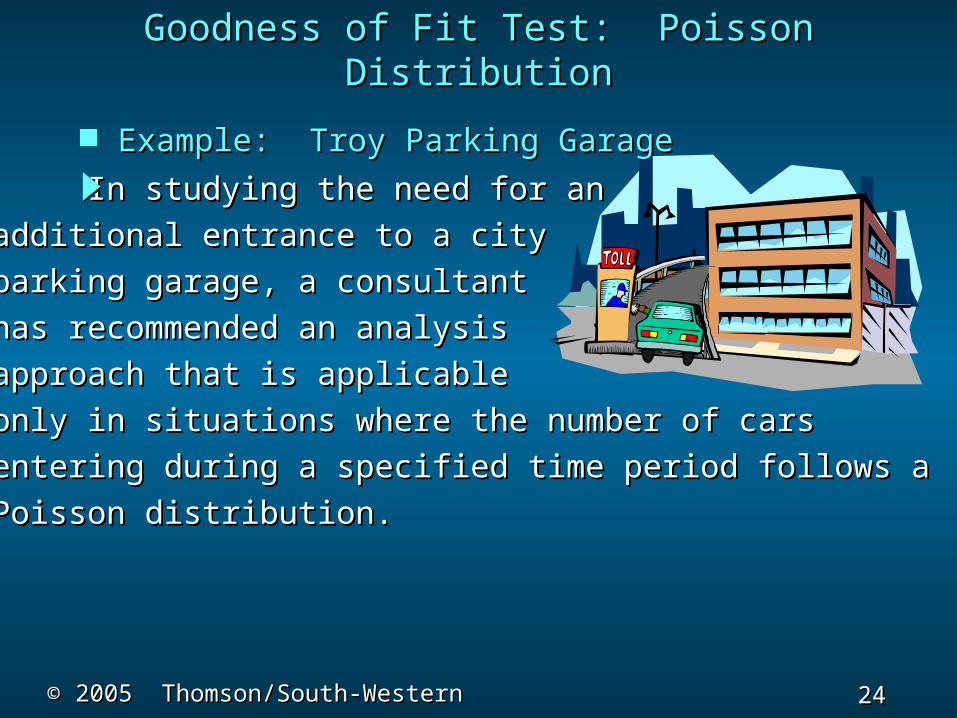
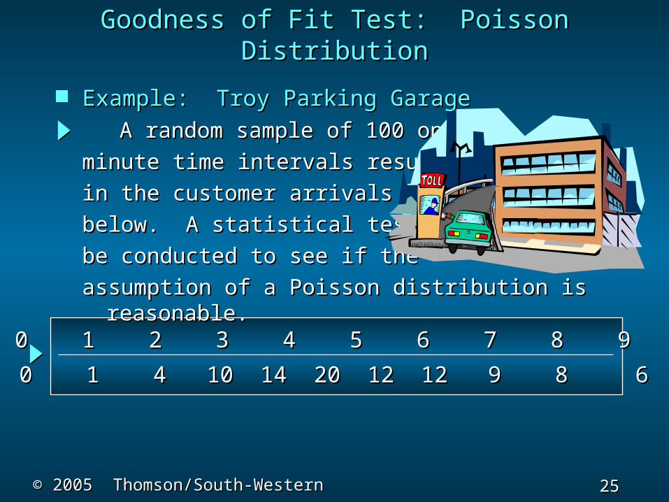
Example: Troy Parking GarageExample: Troy Parking Garage
In studying the need for anIn studying the need for an
additional entrance to a city additional entrance to a city
parking garage, a consultant parking garage, a consultant
has recommended an analysishas recommended an analysis
approach that is applicable approach that is applicable
only in situations where the number of carsonly in situations where the number of cars
entering during a specified time period follows aentering during a specified time period follows a
Poisson distribution.Poisson distribution.
Goodness of Fit Test: Poisson DistributionGoodness of Fit Test: Poisson Distribution
25 25 Slide
Slide
© 2005 Thomson/South-Western© 2005 Thomson/South-Western
A random sample of 100 one-A random sample of 100 one-
minute time intervals resultedminute time intervals resulted
in the customer arrivals listedin the customer arrivals listed
below. A statistical test mustbelow. A statistical test must
be conducted to see if thebe conducted to see if the
assumption of a Poisson distribution is assumption of a Poisson distribution is reasonable.reasonable.
Goodness of Fit Test: Poisson DistributionGoodness of Fit Test: Poisson Distribution
Example: Troy Parking GarageExample: Troy Parking Garage
# Arrivals# Arrivals 0 1 2 3 4 5 6 7 8 9 10 11 120 1 2 3 4 5 6 7 8 9 10 11 12
Frequency 0 1 4 10 14 20 12 12 9 8 6 3 1Frequency 0 1 4 10 14 20 12 12 9 8 6 3 1
26 26 Slide
Slide
© 2005 Thomson/South-Western© 2005 Thomson/South-Western
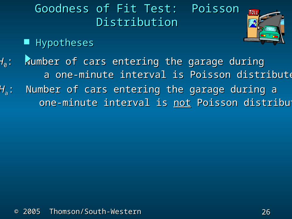
HypothesesHypotheses
Goodness of Fit Test: Poisson DistributionGoodness of Fit Test: Poisson Distribution
HHaa: Number of cars entering the garage during a: Number of cars entering the garage during a one-minute interval is one-minute interval is notnot Poisson distributed Poisson distributed
HH00: Number of cars entering the garage during: Number of cars entering the garage during a one-minute interval is Poisson distributeda one-minute interval is Poisson distributed
27 27 Slide
Slide
© 2005 Thomson/South-Western© 2005 Thomson/South-Western
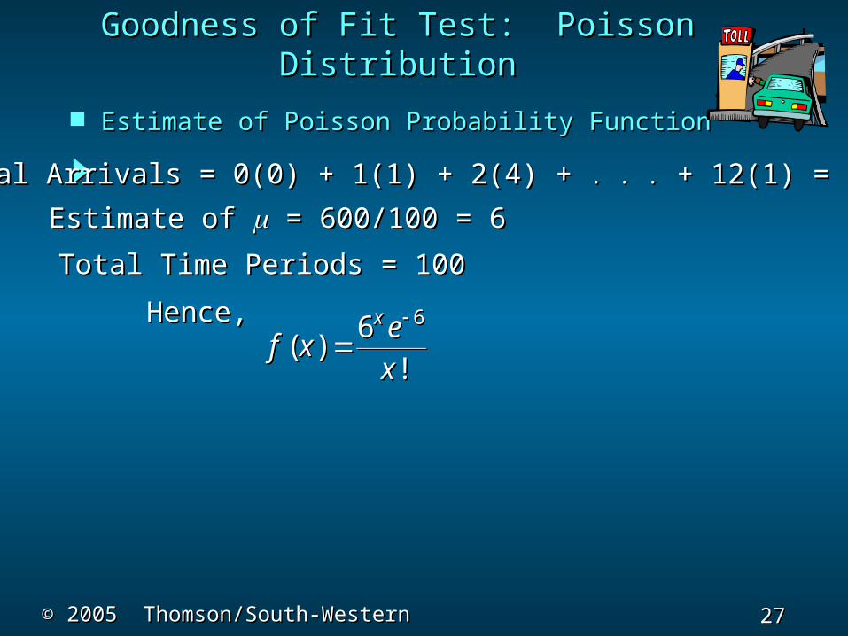
Estimate of Poisson Probability FunctionEstimate of Poisson Probability Function
f xex
x
( )!
6 6
f xex
x
( )!
6 6
f xex
x
( )!
6 6
f xex
x
( )!
6 6
Goodness of Fit Test: Poisson DistributionGoodness of Fit Test: Poisson Distribution
otal Arrivals = 0(0) + 1(1) + 2(4) + otal Arrivals = 0(0) + 1(1) + 2(4) + . . .. . . + 12(1) = 600 + 12(1) = 600
Hence,Hence,
Estimate of Estimate of = 600/100 = 6 = 600/100 = 6
Total Time Periods = 100Total Time Periods = 100
28 28 Slide
Slide
© 2005 Thomson/South-Western© 2005 Thomson/South-Western
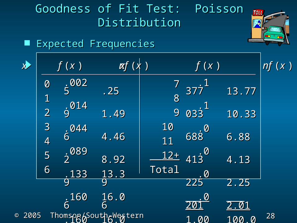
Expected FrequenciesExpected Frequencies
Goodness of Fit Test: Poisson DistributionGoodness of Fit Test: Poisson Distribution
x x f f ((x x ) ) nf nf ((x x ))
00
11
22
33
44
55
66
13.7713.77
10.3310.33
6.886.88
4.134.13
2.252.25
2.012.01
100.0100.000
.137.13777
.103.10333
.068.06888
.041.04133
.022.02255
.020.02011
1.0001.00000
77
88
99
1010
1111
12+12+
TotalTotal
.002.00255
.014.01499
.044.04466
.089.08922
.133.13399
.160.16066
.160.16066
.2.255
1.491.49
4.464.46
8.928.92
13.313.399
16.016.066
16.016.066
xx f f ((x x )) nf nf ((x x ))

29 29 Slide
Slide
© 2005 Thomson/South-Western© 2005 Thomson/South-Western
Observed and Expected FrequenciesObserved and Expected Frequencies
Goodness of Fit Test: Poisson DistributionGoodness of Fit Test: Poisson Distribution
ii ffii eeii ffii - - eeii
-1.20-1.20 1.081.08 0.610.61 3.943.94-4.06-4.06-1.77-1.77-1.33-1.33 1.121.12 1.611.61
6.206.20 8.928.9213.313.39916.016.06616.016.06613.713.77710.310.333 6.886.88 8.398.39
5510101414202012121212 99 881010
0 or 1 or 0 or 1 or 22 33 44 55 66 77 88 9910 or 10 or moremore
30 30 Slide
Slide
© 2005 Thomson/South-Western© 2005 Thomson/South-Western
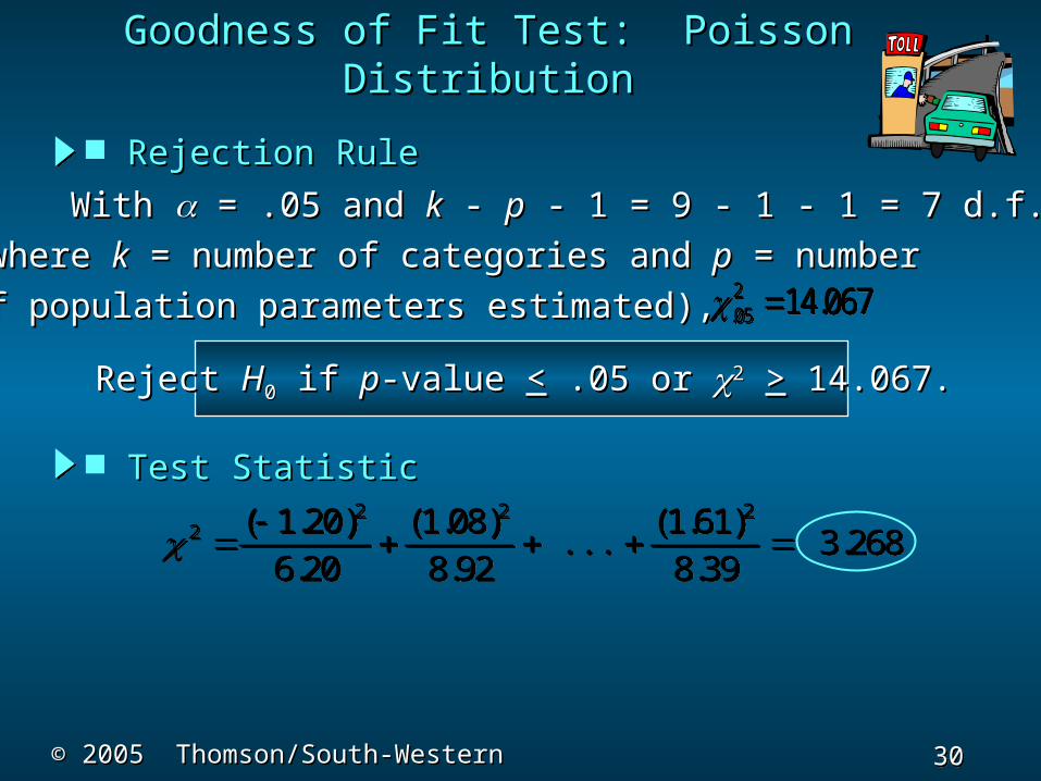
Test StatisticTest Statistic
2 2 22 ( 1.20) (1.08) (1.61)
. . . 3.2686.20 8.92 8.39
2 2 22 ( 1.20) (1.08) (1.61)
. . . 3.2686.20 8.92 8.39
Goodness of Fit Test: Poisson DistributionGoodness of Fit Test: Poisson Distribution
With With = .05 and = .05 and kk - - pp - 1 = 9 - 1 - 1 = 7 d.f. - 1 = 9 - 1 - 1 = 7 d.f.
(where (where kk = number of categories and = number of categories and pp = number = number
of population parameters estimated), of population parameters estimated), 2.05 14.067 2.05 14.067
Reject Reject HH00 if if pp-value -value << .05 or .05 or 22 >> 14.067. 14.067.
Rejection RuleRejection Rule
31 31 Slide
Slide
© 2005 Thomson/South-Western© 2005 Thomson/South-Western
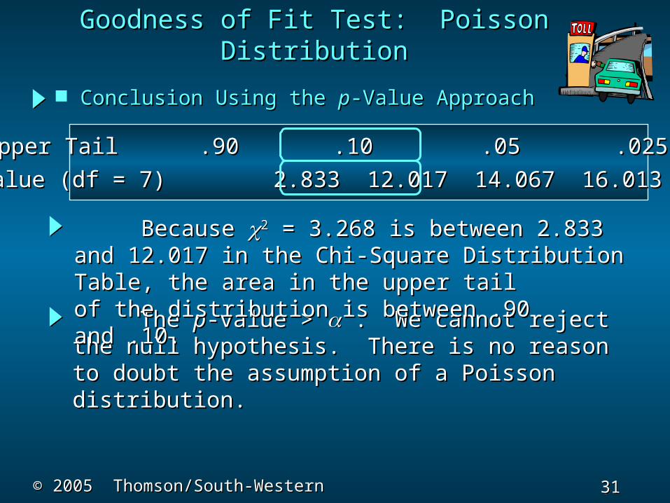
Conclusion Using the Conclusion Using the pp-Value Approach-Value Approach
The The pp-value > -value > . We cannot reject the null . We cannot reject the null hypothesis. There is no reason to doubt the hypothesis. There is no reason to doubt the assumption of a Poisson distribution.assumption of a Poisson distribution.
Because Because 22 = 3.268 is between 2.833 and = 3.268 is between 2.833 and 12.017 in the Chi-Square Distribution Table, the 12.017 in the Chi-Square Distribution Table, the area in the upper tailarea in the upper tailof the distribution is between .90 and .10. of the distribution is between .90 and .10.
Area in Upper Tail .90 .10 .05 .025 .01 Area in Upper Tail .90 .10 .05 .025 .01
22 Value (df = 7) 2.833 12.017 14.067 16.013 18.475 Value (df = 7) 2.833 12.017 14.067 16.013 18.475
Goodness of Fit Test: Poisson DistributionGoodness of Fit Test: Poisson Distribution
32 32 Slide
Slide
© 2005 Thomson/South-Western© 2005 Thomson/South-Western
Goodness of Fit Test: Normal DistributionGoodness of Fit Test: Normal Distribution
1.1. Set up the null and alternative hypotheses. Set up the null and alternative hypotheses.
3.3. Compute the expected frequency, Compute the expected frequency, eei i , for each interval., for each interval.
2.2. Select a random sample and Select a random sample and
a.a. Compute the mean and standard deviation. Compute the mean and standard deviation.
b.b. Define intervals of values so that the expected Define intervals of values so that the expected
frequency is at least 5 for each interval. frequency is at least 5 for each interval.
c.c. For each interval record the observed frequencies For each interval record the observed frequencies
33 33 Slide
Slide
© 2005 Thomson/South-Western© 2005 Thomson/South-Western
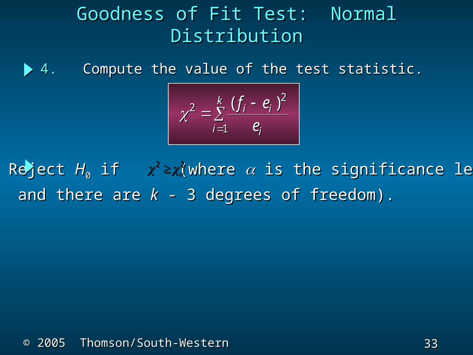
4.4. Compute the value of the test statistic. Compute the value of the test statistic.
Goodness of Fit Test: Normal DistributionGoodness of Fit Test: Normal Distribution
22
1
( )f ee
i i
ii
k2
2
1
( )f ee
i i
ii
k
5.5. Reject Reject HH00 if if (where (where is the significance level is the significance level
and there are and there are kk - 3 degrees of freedom). - 3 degrees of freedom).
2 2 2 2
34 34 Slide
Slide
© 2005 Thomson/South-Western© 2005 Thomson/South-Western
Normal Distribution Goodness of Fit TestNormal Distribution Goodness of Fit Test
Example: IQ ComputersExample: IQ Computers
IQIQIQIQ
IQ Computers (one better than HP?)IQ Computers (one better than HP?)
manufactures and sells a generalmanufactures and sells a general
purpose microcomputer. As part ofpurpose microcomputer. As part of
a study to evaluate sales personnel, a study to evaluate sales personnel, managementmanagement
wants to determine, at a .05 significance level, wants to determine, at a .05 significance level, if theif the
annual sales volume (number of units sold by aannual sales volume (number of units sold by a
salesperson) follows a normal probability salesperson) follows a normal probability distribution.distribution.
35 35 Slide
Slide
© 2005 Thomson/South-Western© 2005 Thomson/South-Western
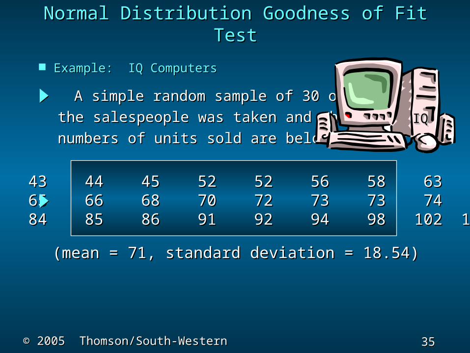
A simple random sample of 30 ofA simple random sample of 30 of
the salespeople was taken and theirthe salespeople was taken and their
numbers of units sold are below.numbers of units sold are below.
Normal Distribution Goodness of Fit TestNormal Distribution Goodness of Fit Test
Example: IQ ComputersExample: IQ Computers
(mean = 71, standard deviation = 18.54)(mean = 71, standard deviation = 18.54)
33 43 44 45 52 52 56 58 63 6433 43 44 45 52 52 56 58 63 6464 65 66 68 70 72 73 73 74 7564 65 66 68 70 72 73 73 74 7583 84 85 86 91 92 94 98 102 10583 84 85 86 91 92 94 98 102 105
IQIQIQIQ

36 36 Slide
Slide
© 2005 Thomson/South-Western© 2005 Thomson/South-Western
HypothesesHypotheses
Normal Distribution Goodness of Fit TestNormal Distribution Goodness of Fit Test
HHaa: The population of number of units sold: The population of number of units sold does does notnot have a normal distribution with have a normal distribution with
mean 71 and standard deviation 18.54.mean 71 and standard deviation 18.54.
HH00: The population of number of units sold: The population of number of units sold has a normal distribution with mean 71has a normal distribution with mean 71 and standard deviation 18.54.and standard deviation 18.54.
37 37 Slide
Slide
© 2005 Thomson/South-Western© 2005 Thomson/South-Western
Interval DefinitionInterval Definition
Normal Distribution Goodness of Fit TestNormal Distribution Goodness of Fit Test
To satisfy the requirement of an To satisfy the requirement of an expectedexpectedfrequency of at least 5 in each interval frequency of at least 5 in each interval we willwe willdivide the normal distribution into 30/5 = divide the normal distribution into 30/5 = 66equal probability intervals.equal probability intervals.

38 38 Slide
Slide
© 2005 Thomson/South-Western© 2005 Thomson/South-Western
Interval DefinitionInterval Definition
Areas = 1.00/6 = .1667
Areas = 1.00/6 = .1667
717153.0253.02
71 .43(18.54) = 63.0371 .43(18.54) = 63.0378.9778.9788.98 = 71 + .97(18.54)88.98 = 71 + .97(18.54)
Normal Distribution Goodness of Fit TestNormal Distribution Goodness of Fit Test

39 39 Slide
Slide
© 2005 Thomson/South-Western© 2005 Thomson/South-Western
Observed and Expected FrequenciesObserved and Expected Frequencies
Normal Distribution Goodness of Fit TestNormal Distribution Goodness of Fit Test
11
-2-2
11
00
-1-1
11
55
55
55
55
55
55
3030
66
33
66
55
44
66
3030
Less than 53.02Less than 53.02
53.02 to 63.0353.02 to 63.03
63.03 to 71.0063.03 to 71.00
71.00 to 78.9771.00 to 78.97
78.97 to 88.9878.97 to 88.98
More than 88.98More than 88.98
ii ffii eeii ffii - - eeii
TotalTotal

40 40 Slide
Slide
© 2005 Thomson/South-Western© 2005 Thomson/South-Western
2 2 2 2 2 22 (1) ( 2) (1) (0) ( 1) (1)
1.6005 5 5 5 5 5
2 2 2 2 2 22 (1) ( 2) (1) (0) ( 1) (1)
1.6005 5 5 5 5 5
Test StatisticTest Statistic
With With = .05 and = .05 and kk - - pp - 1 = 6 - 2 - 1 = 3 d.f. - 1 = 6 - 2 - 1 = 3 d.f.
(where (where kk = number of categories and = number of categories and pp = number = number
of population parameters estimated), of population parameters estimated), 2.05 7.815 2.05 7.815
Reject Reject HH00 if if pp-value -value << .05 or .05 or 22 >> 7.815. 7.815.
Rejection RuleRejection Rule
Normal Distribution Goodness of Fit TestNormal Distribution Goodness of Fit Test
41 41 Slide
Slide
© 2005 Thomson/South-Western© 2005 Thomson/South-Western
Normal Distribution Goodness of Fit TestNormal Distribution Goodness of Fit Test
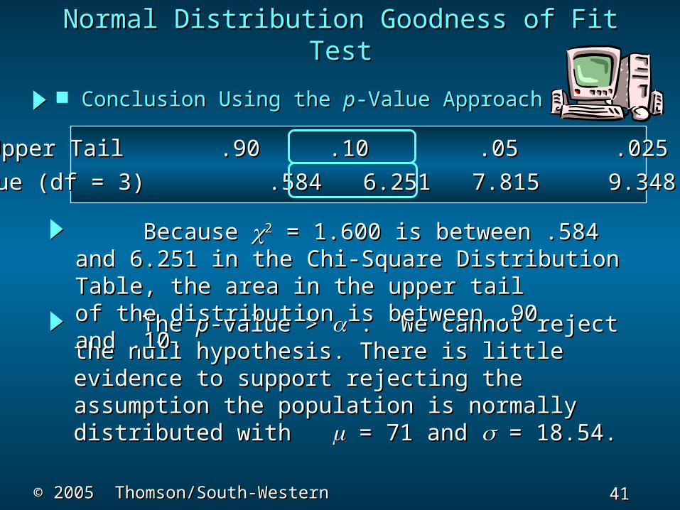
Conclusion Using the Conclusion Using the pp-Value Approach-Value Approach
The The pp-value > -value > . We cannot reject the null . We cannot reject the null hypothesis. There is little evidence to support hypothesis. There is little evidence to support rejecting the assumption the population is rejecting the assumption the population is normally distributed with normally distributed with = 71 and = 71 and = 18.54. = 18.54.
Because Because 22 = 1.600 is between .584 and = 1.600 is between .584 and 6.251 in the Chi-Square Distribution Table, the 6.251 in the Chi-Square Distribution Table, the area in the upper tailarea in the upper tailof the distribution is between .90 and .10. of the distribution is between .90 and .10.
Area in Upper Tail .90 .10 .05 .025 .01 Area in Upper Tail .90 .10 .05 .025 .01
22 Value (df = 3) .584 6.251 7.815 9.348 11.345 Value (df = 3) .584 6.251 7.815 9.348 11.345

42 42 Slide
Slide
© 2005 Thomson/South-Western© 2005 Thomson/South-Western
End of Chapter 12End of Chapter 12
Related Documents