1-1 Copyright © 2015, 2010, 2007 Pearson Education, Inc. Chapter 13, Slide 1 Chapter 13 From Randomness to Probability.

1-1 Copyright © 2015, 2010, 2007 Pearson Education, Inc. Chapter 13, Slide 1

Chapter 13From Randomness

to Probability


Dealing with Random Phenomena A random phenomenon is a situation in which we

know what outcomes could happen, but we don’t know which particular outcome did or will happen.

In general, each occasion upon which we observe a random phenomenon is called a trial.

At each trial, we note the value of the random phenomenon, and call it an outcome.

When we combine outcomes, the resulting combination is an event.

The collection of all possible outcomes is called the sample space.


Independence (again)

First a definition . . . When thinking about what happens with

combinations of outcomes, things are simplified if the individual trials are independent. Roughly speaking, this means that the outcome

of one trial doesn’t influence or change the outcome of another.

For example, coin flips are independent.


The Law of Large Numbers

The Law of Large Numbers (LLN) says that the long-run relative frequency of repeated independent events gets closer and closer to a single value.

We call the single value the probability of the event.

Because this definition is based on repeatedly observing the event’s outcome, this definition of probability is often called empirical probability.


The Nonexistent “Law of Averages”

The LLN says nothing about short-run behavior. Relative frequencies even out only in the long run,

and this long run is really long (infinitely long, in fact).

The so called Law of Averages (that an outcome of a random event that hasn’t occurred in many trials is “due” to occur) doesn’t exist at all.


The probability of an event is the number of outcomes in the event divided by the total number of possible outcomes.

P(A) =

Modeling Probability (cont.)

# of outcomes in A

# of possible outcomes


Formal Probability

1. Two requirements for a probability: A probability is a number between 0 and 1. For any event A, 0 ≤ P(A) ≤ 1.


Formal Probability (cont.)

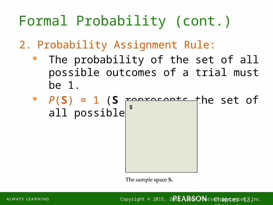
2. Probability Assignment Rule: The probability of the set of all possible

outcomes of a trial must be 1. P(S) = 1 (S represents the set of all possible

outcomes.)



3. Complement Rule: The set of outcomes that are not in the event

A is called the complement of A, denoted AC. The probability of an event occurring is 1

minus the probability that it doesn’t occur: P(A) = 1 – P(AC)



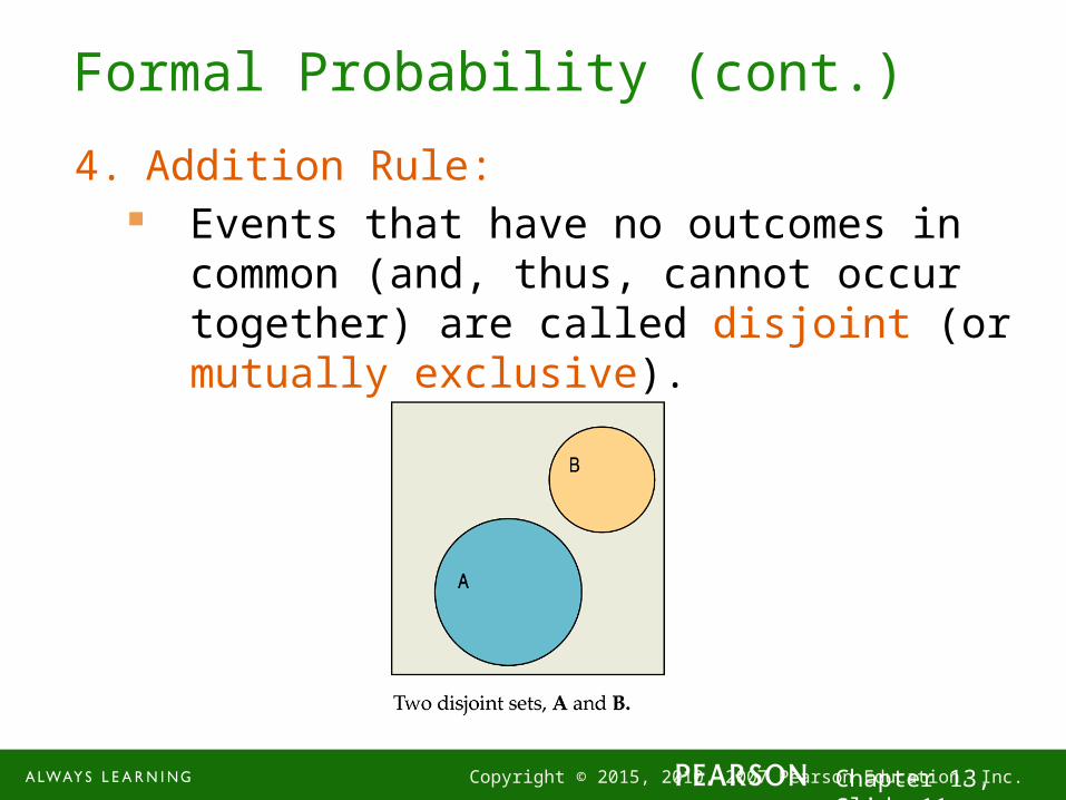
4. Addition Rule: Events that have no outcomes in common

(and, thus, cannot occur together) are called disjoint (or mutually exclusive).



4. Addition Rule (cont.): For two disjoint events A and B, the

probability that one or the other occurs is the sum of the probabilities of the two events.

, provided that A and B are disjoint.P(AB)P(A)P(B)



5. Multiplication Rule: For two events A and B, the probability that

both A and B occur is the product of the probabilities of the two events.

means the probability of B given A. If the two events are independent this is the same as the probability of B

For independent events,

( ) ( ) ( | )P A B P A P B A

( | )P B A

( ) ( ) ( )P A B P A P B



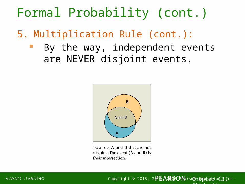
5. Multiplication Rule (cont.): By the way, independent events are NEVER

disjoint events.



5. Multiplication Rule: Many Statistics methods require an

Independence Assumption, but assuming independence doesn’t make it true.

Always Think about whether that assumption is reasonable before using the Multiplication Rule.


Formal Probability - Notation

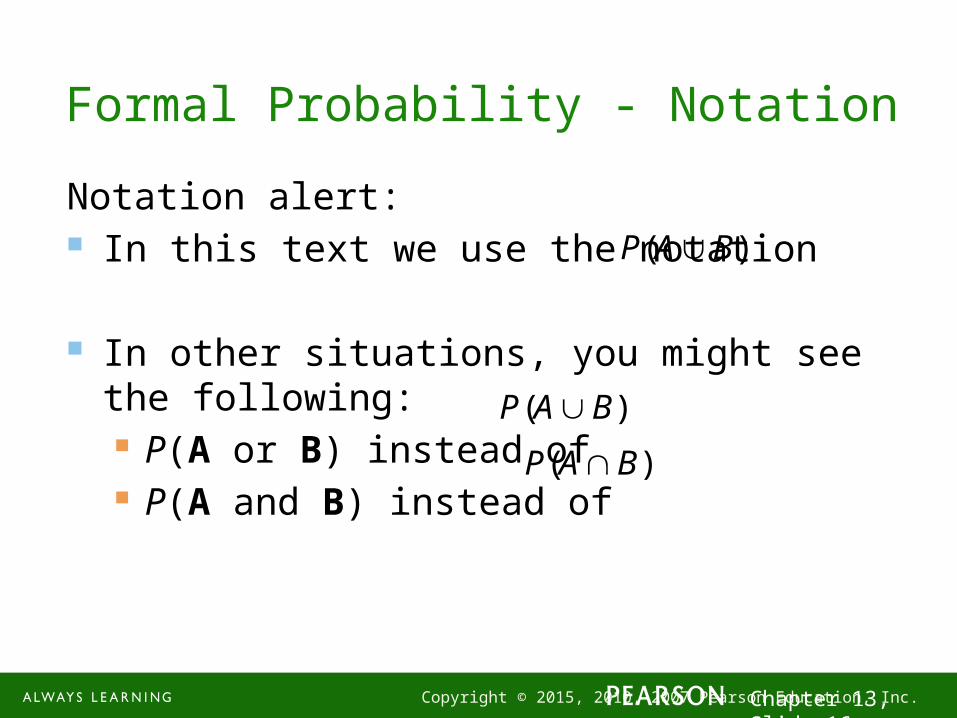
Notation alert: In this text we use the notation

In other situations, you might see the following: P(A or B) instead of P(A and B) instead of

P(AB)

P(AB)

P(AB)


What Can Go Wrong?

Beware of probabilities that don’t add up to 1. To be a legitimate probability distribution, the

sum of the probabilities for all possible outcomes must total 1.

Don’t add probabilities of events if they’re not disjoint. Events must be disjoint to use the Addition

Rule.


What Can Go Wrong? (cont.)

Don’t confuse disjoint and independent—disjoint events can’t be independent.


What have we learned?

Probability is based on long-run relative frequencies.

The Law of Large Numbers speaks only of long-run behavior. Watch out for misinterpreting the LLN.


What have we learned? (cont.)

There are some basic rules for combining probabilities of outcomes to find probabilities of more complex events. We have the: Probability Assignment Rule Complement Rule Addition Rule for disjoint events Multiplication Rule for independent events


AP Tip

For even the most simple probability problem, always show work. It may even just be to show the fraction that you used to calculate the percent.

1-1 Copyright © 2015, 2010, 2007 Pearson Education, Inc. Chapter 13, Slide 1 Chapter 13 From Randomness to Probability.

Documents

probability slide

pearson education

definition of probability

formal probability

modeling probability

empirical probability

number of outcomes

random event