ED 0 58 668 AUTHOR TITLE INSTITUTION REPORT NO PUB DATE CONTRACT NOTE AVAILABLE FROM EDRS PRICE DESCRIPTORS DOCUMENT RESUME EA 004 049 Jaffe, A. J. Handbook of Statistical Procedures for Long-Range Projections of Public School Enrollment. Technical Monograph. Office of Education (DREW) Washington, D.C. 0E-24017 69 OEC-1-7-701253-5103 131p. Superintendent of Documents, U.S. Government Printing Of fice, Washington, D.C. 20402 (Catalog No. HE 5.224:24017, $1.25) MF-$0.65 HC-$6.58 Educational Planning; *Educational Trends; *Enrollment Projections; Enrollment Trends; School Districts; School Planning; *School Statistics; Statewide Planning; *Statistical Analysis; Statistical Data; *Trend Analysis ABSTRACT This handbook presents statistical procedures that will assist State and local school officials in making longrange projections for a decade or more. The author suggests several seemingly appropriate procedures but leaves it to the State and local officials to select the procedures that appear most suitable for their specific local conditions. This document is organized around eight chapters that (1) make general observations on statistical projections, (2) examine local school district histories to appraise the problem of applying statistical projection techniques to them, (3) present some summary materials on procedures for making shortrun projections, (4) discuss methods for making unified projections for the State and all its political units, and (5) present materials to aid local districts in making longrange projections. (Author/JF)

Welcome message from author
This document is posted to help you gain knowledge. Please leave a comment to let me know what you think about it! Share it to your friends and learn new things together.
Transcript
ED 0 58 668
AUTHORTITLE
INSTITUTIONREPORT NOPUB DATECONTRACTNOTEAVAILABLE FROM
EDRS PRICEDESCRIPTORS
DOCUMENT RESUME
EA 004 049
Jaffe, A. J.Handbook of Statistical Procedures for Long-RangeProjections of Public School Enrollment. TechnicalMonograph.Office of Education (DREW) Washington, D.C.0E-2401769OEC-1-7-701253-5103131p.Superintendent of Documents, U.S. Government PrintingOf fice, Washington, D.C. 20402 (Catalog No. HE5.224:24017, $1.25)
MF-$0.65 HC-$6.58Educational Planning; *Educational Trends;*Enrollment Projections; Enrollment Trends; SchoolDistricts; School Planning; *School Statistics;Statewide Planning; *Statistical Analysis;Statistical Data; *Trend Analysis
ABSTRACTThis handbook presents statistical procedures that
will assist State and local school officials in making longrangeprojections for a decade or more. The author suggests severalseemingly appropriate procedures but leaves it to the State and localofficials to select the procedures that appear most suitable fortheir specific local conditions. This document is organized aroundeight chapters that (1) make general observations on statisticalprojections, (2) examine local school district histories to appraisethe problem of applying statistical projection techniques to them,
(3) present some summary materials on procedures for making shortrunprojections, (4) discuss methods for making unified projections forthe State and all its political units, and (5) present materials toaid local districts in making longrange projections. (Author/JF)
Technical Monograph Project Contract No. OEC-1-7-701253-5103 0E-24017
U.S. DEPARTMENT OF HEALTH.EDUCATION & WELFAREOFFICE OF EDUCATION
THIS DOCUMENT HAS BEEN REPRO.
DUCE() EXACTLY AS RECEIVEO FROM
THE PERSON OR ORGANIZATION ORIG.
INATING IT. POINTS OF VIEW OR OPIN.
OZ3)
IONS STATED DO NOT NECESSARILYREPRESENT OFFICIAL OFFICE OF EDU.
CATION POSITION OR POLICY.
5 HANDBOOK OFSTATISTICAL PROCEDURESFOR LONG-RANGE PROJECTIONSOF PUBLIC SCHOOL ENROLLMENT
by A. J. JaffeBureau ol Applied Social Research, Columbia University
&I U.S. DEPARTMENT OF HEALTH, EDUCATION, AND WELFARE
Office of Program Planning and Evaluation
1
Office of Education
The research reported herein was performed pursuant to a contract with the Officeof Education, U.S. Department of Health, Education, and Welfare. Contractorsundertaking such projects under Government sponsorship arc encouraged to expressfreely their professional judgment in thc conduct of the project. Points of view oropinions stated do not, therefore, necessarily represent official Office of Educationposition or policy.
Superintendent of Documents Catalog No. HE 5.224 :24017
U.S. GOVERNMENT PRINTING OFFICEWASHINGTON : 1969
For sale by the Superintendent of Documents, U.S. Govenunent Printing 011iceWashington, D.C. 20102 - Price $1.25
FOREWORD
It is expected that this methodology handbook will be of considerable aid
to State and local school officials in preparing long-range enrollment estimates.
A lead time of several years is often required to build or enlarge facilities,
obtain staff, and plan educational programs.Dr. A. J. Jaffe, Direct.r of the Manpower and Population Program of
Columbia University's Bureau of Applied Social Research, is a well-knowndemographer and statistician. Among his many writings is the Handbook ofStatistical Methods for Demographers, published by the U.S. Census Bureau (and
issued by the Government Printing Office in 1951). Any reader who is inter-
ested in pursuing the various methldological problems of making projections
could profitably refer to this earlier volume.Dr. Jaffe introduces in the present volume a variety of statistical methods
which are applicable to different situations. The author suggests the use ofseveral procedures which may be most appropriate under different conditionsin a school district, but the reader must select the procedures which appear to
him to be most useful for his situation. Local conditions are so variable that
no hard and fast and immutable "rules" can be laid down. Each official using
this volume must take into consideration his knowledge about his State orlocal conditions, select the methodor methodswhich he wants to use tomake forecasts, and then interpret the resulting statistical projections in lightof his intimate knowledge of his partitmlar conditions. Fortunately, enough
States and local school districts have enough in common so that a few generalprocedures will fit most projection needs.
June 1969
JOSEPH FROOMKIN,
Assistant Commissioner for Program Planning and Evaluation,Office of Education.
PREFACE
State and local school officials need estimates of long-range future enroll-
ment in public schools for a variety of planning purposes. Accordingly, we are
here presenting an array of statistical procedures which can be used for making
projections a decade or longer into the future.There is no statistical formula which will foretell the future precisely. The
best that we can hope to at Lain is some reasonable estimate which may serve
as a basis for drawing plans for construction, recruitment of teachers, and so
forth. The statistical prccedures for obtaining this "reasonable estimate" vary
greatly from one State or local school district, to imother insofar as the history,
conditions, and information available for each area are different from others.
Therefore, we present a variety of methods with suggestions as to the type of
condition under which each may be most appropriate. The State and local
school officials must, then choose that method, or methods, which seems most
suitable for theiv specific local conditions.After applying that "best" procedure and obtaining a long-range projec-
tion, State and local school officials must then evaluate the statistical results
in light of all their knowledge of the local community. No statistical formula
can take into consideration every item of knowledge available to the local
residents. Therefore the judgment of the State and local officials, based on
their intimate knowledge of local conditions, must be applied to an appraisal
of any statistical results.This Handbook is organNed as follows: In chapter 1, we make some
general observations on statistical projections. In chapter 2, we examine the
history of local school districts in the United States in an effort to appraise
the general problem of nvoiying statistical projection techniques to them.
Chapters 3 and 4 present some summary materials on the procedures for
making shortrun projections. All of these methods have been used by local
school districts and States, and work well in the short run. However, they are
of questionable value for longrun projections.In chapters 5, 6, and 7, we discuss methods for making unified projections
for the State and all its political units. We reason as follows: It is relatively
easy to make reasonably accurate projections for a State since it is such a
large unit. True, some States, such as California, pose methodological problems
because of the unusually largo nmnber of in-migrants; nevertheless, it is easier
to estimate future migration into the entire State than into any particular part
of it. Therefore, we first project school enrollment for the entire State.
Wo also know that the total number of pupils enrolled in each of the
public schools of the State must equal the total number enrolled in the State.
Therefore, we can use the projected number in the State as a standard in calcu-
lating the projected number in each local political unit. By equating the sum
of tho local units with the State total, we reduce the average error in each
political subunit. Chapter 5 contains a discussion of this.
Not all States will prepare unified projections for their subdivisions.
In some cases, local school districts will find it necessary to prepare their own
projections. Chapter 8 presents some materials which will aid the local districts
to make long-range projections. We prefer the unified projections, but if theyare not available, then the procedures outlined in chapter 8 can be substituted.
Finally, several appendixes are included, containing additional method-ological materials.
June 1969
vi
DR. A. J. JAFFE,Director of the Manpower and Population Program,
Columbia University, Bureau of Applied Social Research.
ACKNOWLEDGMENTS
We gratefully acknowledge the support, advice, and technical assistance
given us during the course of the preparation of the handbook by a number of
individuals in the U.S. Office of Education, several State and local district
offices of education, the New England Education Data Systems, the Southern
Regional Education Board, the U.S. Bureau of the Census, and the State of
California, Population Research Unit.
U.S. Office of Education.Dr. Joseph Froomkin, Assistant Commissioner
for Program Planning and Evaluation, Mrs. Cora P. Beebe, Special Assistant,
Office of Program Planning and Evaluation; Dr. Kenneth A. Simon and Dr.
Stanley Smith, National Center for Educational Statistics.
State Departments of EducationConnecticut.Dr. Maurice J. Ross, Chief, Bureau of Research, Statistics
and Finance.Maryland.Dr. Richard D. McKay, Director, and Miss Catherine Hogan,
Division, Research and Statistics.Massachusetts.Dr. James R. Baker, Assistant Commissioner for
Research and Development, and Dr. George J. Collins, Assistant Commissioner
for School Facilities and Related Services.New Jersey.Dr. S. David Winans, Director, Office of Statistical Services.
New York.Dr. Lorne H. Wool lett, Associate Comnissioner for Research
and Special Studies; Dr. John J. Stiglmeier, Director, and Dr. Joseph Lev,
Chief Statistician, Bureau of Statistical Services.Rhode Island.Edward F. Wilcox, Associate Commissioner of Education.
Local School officesSacramento, Calif.Walter A. Parsons, Sacramento Unified School
District.Montgomery County, Md.Henry J. Hilburn, Director of Planning,
Montgomery County Educational Services Administration.
Independent Educational Agencies.E. F. Shietinger, Southern Regional
Education Board, Atlanta, Ga. Michael Wilson and John Sullivan, New
England Educational Data Systems, Cambridge, Mass.
Other Federal and State Agencies.Meyer Zitter, State and Local Pop-
ulation Estimates, U.S. Bureau of the Census, Suit land, Md. for providing
several unpublished State population projection series prepared by the Census
Bureau and used in chapters 6 and 7. Walter Holmann, Director, Joseph Freitas,
Deputy Director, and Mrs. Isabel Hambright, Population Research Unit,
Dep artment of Finance, State of California, Sacramento, for providing un-
published and published series of population projections for California and used
in chapters 6 and 7.
OthersIn addition, we wish to thank the following persons from Columbia
University: Jerome B. Gordon, who assisted on all phases of this handbook ;
Dr. John U. Farley and Joseph Lopatin for assistance with the exponential
smoothing procedures shown in chapter 7 and appendix C; Melvin 1.4008 for his
editorial efforts; and Fred Morgan and Orlando Rodriguez for their clerical and
statistical assistance in the preparation of various parts of this report.vii
Finally, we wish to thank the following for permission to quote from theirworks:
Connecticut State Department of Education, Maurice J. Ross, Chief,Bureau of Research, Statistics and Finance, Hartford, Conn. Instructions ,forUsing the Estimate qf Future Enrollments and Connecticut's Need ,for NewTeachers, 1968-1982 (Research Bulletin No. 3, April 1967).
John K. Folger and the Southern Regional Education Board, "CohortSurvival Method" Chapter 1V of a mimeographed, undated Southern RegionalEducation Board report entitled Some Methods ,for Projecting School and CollegeEnrollments by John K. Folger.
Dr. Francis Duehay and the Harvard University Graduate School ofEducation, Watertown: Its Schools and Needs, Cambridge, 1966.
Dr. E. Brewin, Dr. A. R. Post, and the Fels Institute of Local and StateGovernment, University of Pennsylvania, Estimate of Future PopulationGrowth by School District, Ducks County, Pa., June 1967.
viii
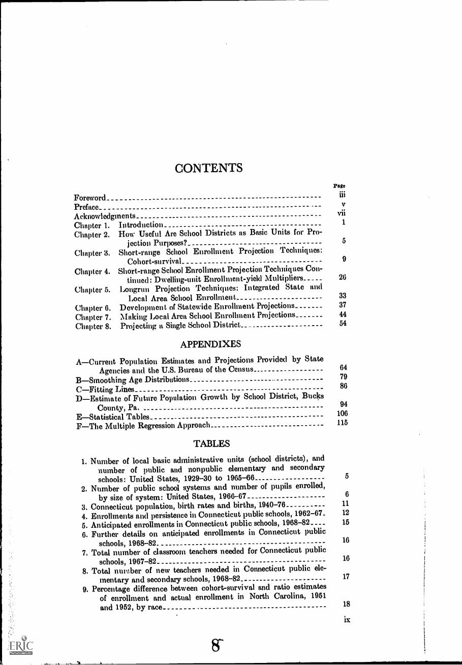
CONTENTSPage
ForewordPrefaceAcknowledgments vii
Chapter 1. Introduction _1
Chapter 2. How Useful Are School Districts as Basic Units for Pro-jection Purposes? 5
Chapter 3. Short-range School Enrollment Projection Techniques:Cohort-survival 9
Chapter 4. Short-range School Enrolhnent Projection Techniques Con-tinued : Dwelling-unit Enrollment-yield Multipliers 26
Chapter 5. Longrun Projection Techniques: Integrated State andLocal Area School Enrollment 33
Chapter 6. Development of Statewide Enrollment Projections 37
Chapter 7. Making Local Area School Enrollment Projections 44
Chapter 8. Projecting a Single School District_ 54
APPENDIXES
ACurrent Population Estimates and Projections Provided by StateAgencies and the U.S. Bureau of the Census_ 64
BSmoothing Age Distributions 79
CFitting Lines 86
DEstimate of Future Population Growth by School District, BucksCounty, Pa. 94
EStatistical Tables 106
FThe Multiple Regression Approach 115
TABLES
1. Number of local basic administrative units (school districts), andnumber of public and nonpublic elementary and secondaryschools: United States, 1929-30 to 1965-66 5
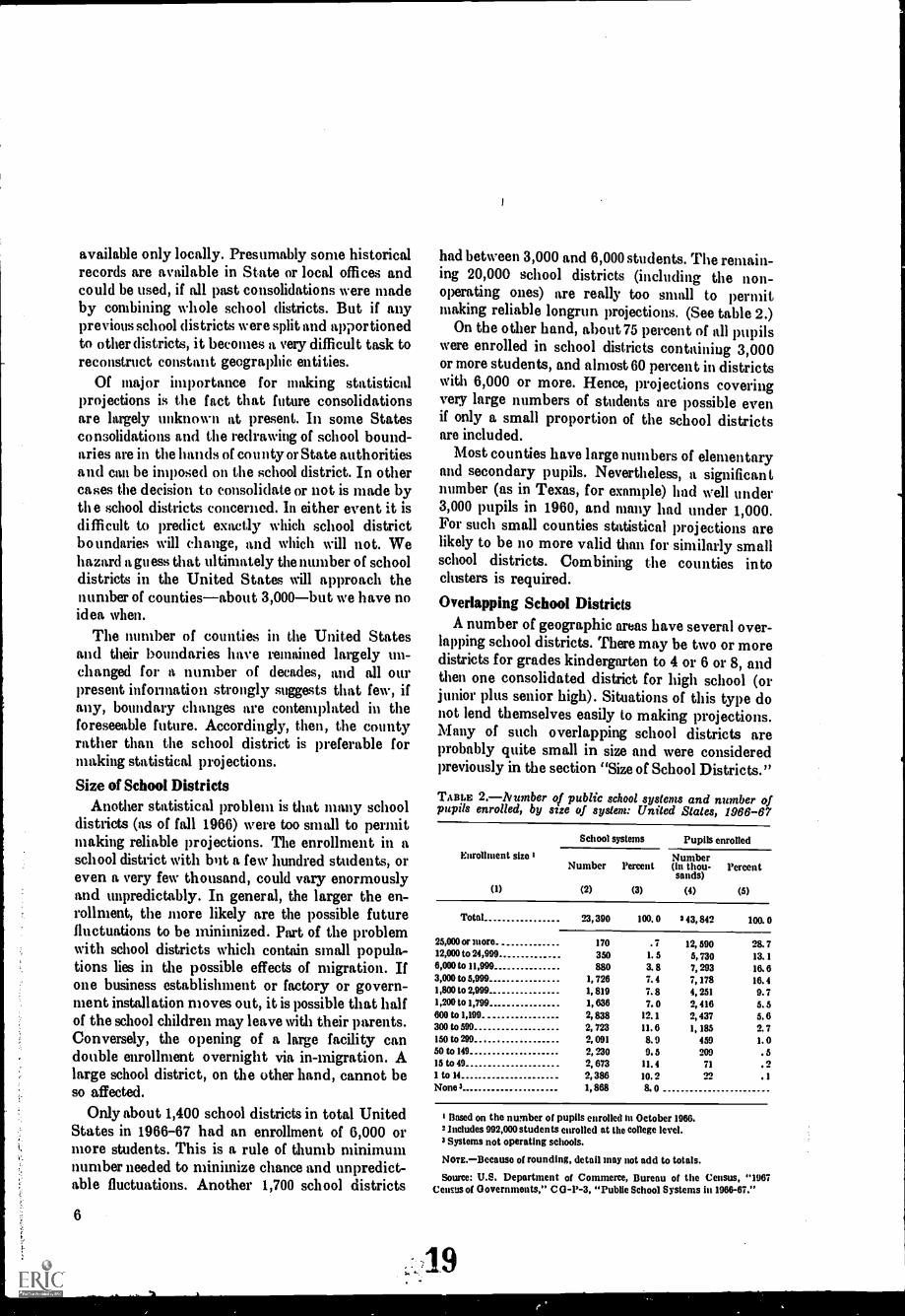
2. Number of public school systems and number of pupils enrolled,by size of system: United States, 1966-67 6
3. Connecticut population, birth rates and births, 1940-76 11
4. Enrollments and persistence in Connecticut public schools, 1962-67_ 12
5. Anticipated enrollments in Connecticut public schools, 1968-82.. _ _ _ 15
6. Further details on anticipated enrollments in Connecticut publicschools, 1968-82. 16
7. Total number of classroom teachers needed for Connecticut publicschools, 1967-82 16
8. Total number of new teachers needed in Connecticut public ele-mentary and secondary schools, 1968-82 17
9. Percentage difference between cohort-survival and ratio estimatesof enrollment and actual enrollment in North Carolina, 1951and 1952, by race 18
ix
84-
Page
10. Percentage difference between cohort-survival and ratio estimatesof enrollment and .actual enrollment in South Carolina, 1951and 1952, by race 18
11. Alabama white elementary enrollment_ 1912. Adjustment of births for under-registration and to a school-year
basis 2013. Computation of survival ratios, births to second grade enrollment,
Alabama whites 2014. Distribution of Watertown children in public and nonpublic schools_ 2115. Construction of new dwelling units 2116. Age distribution of women 2217. Percentage of survival 2218. 1970 predicted age distribution of women. 2219. Women in Watertown by age group, 1966-71 2220. Number of births in Watertown, 1950-65 2321. Fertility ratios 2322. Projected births by age group, 1966-71 2423. Average percentage of survivals_ 2524. Projections of Watertown public school enrollments by grade,
1967-76 2525. Projections of enrollments in 4-4-4 organizational patterns, 1967-76.. 2526. Public student yields per residential dwelling unit, Montgomery
County, Md. 2927. Structure, component methodology and projection possibilities of
integrated State-local area school enrollment long-range pro-jection technique 35
28. Age by sex by grade, public school enrollment, State of Maryland,1960 38
29. Age-grade nmtrix, proportions enrolled in public school, both sexes,State of Maryland, 1960 38
30. Computations for projecting 1960 age-grade matrix of public schoolenrollment, States of Maryland and California 40
31. State of Maryland projected age-grade matrices, 1965-80 4032. State of California projected proportion enrolled in public schools,
ages 18 and 19 4033. Projection of age-grade public school enrollment ratios, ages 14-15
and 16-17, for grades 9-12, United States 41
34. Steps in projecting 1965 public school enrollment, State of Mary-land 42
35. Comparison of actual versus projected public school enrollment,States of Maryland and California, 1965, grades 4-4-4 42
36. 1980 projections of statewide public. school enrollments, by gradegroups, States of Maryland and California 43
37. Actual and projected enrollment shares by county, "4-4-4" organiza-tion of enrollment, State of Maryland, 1965 49
38. Actual and projected absolute enrollments by county, "4-4-4"organization of enrollmert, State of Maryland, 1965 50
39. Summary comparisons el projected and observed shares and enroll-ment, by grade grorips, by counties, Maryland, 1965 50
40. Projected public schoul fall enrollment shares by grade group andcounty, and methods of adjustment, State of Maryland, 1980_ _ _ _ 51
Page
41. 1980 projected enrollment by grade groups, State of Maryland, by
counties 51
42. Actual and projected enrollment shares by area, "4-4-4" organiza-
tion of enrollment, State of California, 1965 52
43. Projected public school fall enrollment shares by grade group andarea, and method of adjustment, State of California, 1980_ _ _ _ 53
44. Projected enrollment by grade groups, State of California, by areas,
1980 53
45. Projecting school districts 1960 to 1980, an example using New.
Jersey 56
46. Work sheet for calculating projection equations for table 45 57
47. Procedures for converting population, aged 5 to 17, to numbersenrolled in public schools, grades 1 to 12, for counties, hypothetical
data 58
48. Procedures for projecting local school district enrollment fromestimated county enrollment data, grades 1 to 12, hypotheticaldata 59
EXHIBITS
1. Connecticut State Department of Education, Bureau of Research,Statistics, and Finance, Estimate of future enrollments 13
2. Anticipated enrollments in Connecticut public schools 15
3. Total number of classroom teachers needed for Connecticut public
schools 16
4. Total number of new teachers needed in Connecticut elementary and
secondary public schools 17
5. Projected average daily attendance 30
6. Projected average daily attendance 31
7. 7-year projection of A.D.A. (for purchase of sites) 32
8. MarylandCounties, places of 25,000 or more, and standard metro-politan statistical areas 46
9. California State statistical areas 47
APPENDIX TABLES
A-1. State agencies making population estimates for local areas:Periodic surveys, 1955 to 1965 65
A-2. Methods used by State agencies to make population estimatesfor local areas: Survey of 1965 66
A-3. Summary of methods used by State agencies to make populationestimates for local areas: Periodic surveys, 1955 to 1965 66
A-4. Population estimates prepared by State agencies: Survey of1965 68
A-5. Projected fertility rates, by color: 1960-65 to 1980-85 73
A-6. Rate of total net migration (in percent) for selected States: 1955-65, 1965-75, 1975-85 76
B-1. Estimating single years of age, using mid-panel of the Spraguemultipliers, age 20 to 24 years token as an example.. 80
B-2. Estimating single years of age using end-panels of the Spraguemultipliers 81
xi
10
CHAPTER 3
SHORT-RANGE SCHOOL ENROLLMENT
PROJECTION TECHNIQUES: COHORT-SURVIVAL
Perhaps one of the most frequently used tech-niques in the projection of school enrollments is
the cohort-survival or grade persistence method.The technique derives its name from the use of
grade-to-grade survival or persistence ratios,easily computed from historical series of enroll-
ment by individual gradesdata which most localschool districts and State departments ofeducationshould have on hand.
Basically, only two inputs are required to makeenrollment forecasts using the technique. Thefirst is the number of residential births for the
State or local school district, which is obtainedfrom vital statistics data compiled by local orState boards or departments of health. The secondis the array of projections of grade-to-grade sur-vival ratios; for example, the probabilities orchances of a given cohort of new enrollees "sur-viving" from birth to kindergarten, or from fifthto sixth grade. The grade-survival ratios may beless or more than one, or unity. Grade-survivalratios of less than one indicate the net effectsof deaths, out-transfers to private schools, netout-migration from the community, or dropouts.Grade-survival ratios of more than one indicate thenet effects of in-transfers from private schools andnet in-migration into the State or community.Projections of enrollments are made by applying,consecutively, the individual grade-to-grade-sur-vival ratio to each entering cohortfor example,new enrollees in kindergarten to first grade.
The simplest version of the cohort-survivalmethod can be illustrated as follows: Supposethat in 1960, 1,000 infants are born in communityX. In 1965, 800 enter kindergarten. The survivalratio from birth to kindergarten is 800 divided by1,000, or .80.
Next, suppose that in 1965 there were 600children in kindergarten, and in 1966, 650 in first
2
grade. The survival ratio from kindergarten tofirst grade is 1.083.
These ratios can be calculated between eachtwo grades all the way to graduation from highschoolcompletion of the 12th grade.
Furthermore, in an effort to obtain more stableratios, the numbers can be averaged for severalyears. Thus, in the appended article, "Con-necticut's Need for New Teachers, 1968-1982,"5-year enrollment averages were used (table 4 ofarticle).
Long-Range Projection Difficulties
Long-range projections can be made by simplycontinuing the process of applying the survivalratios until, at least, those alive at the initialdate have completed the 12th year of school;the arithmetic is simple. One major problemwhich arises in making long-range projections isthat of estimating future numbers of births inorder to begin the successive entry cohorts, forexample, the numbers in kindergarten or firstgrade at each successive year. This is a complicatedjob, and to do it properly requires more personneland machine resources than most school districtshave available. On the other hand, the methodsto be proposed in chapters 5 to 8 make full use of
the long-range population projections which theCensus Bureau has prepared, thus greatly mini-mizing the work required at the local level.
A second major problem is that of estimatingthe future population of school-going-age whichwill live within that school district. Simpleextrapolation of the survival ratios assumes thatthere will be no drastic changes in the volume ordirection of migration. Yet extensive in- or out-migration can affect the survival ratio. (Drasticchange in the balance of public and privateschool enrollment can also alter the survival
9
Page
B-3. Estimating single years of age using next-to-end-panels of theSprague multipliers_ 82
B-4. Estimating percent of single marital status, by single years ofage, using Sprague mid-panel multipliers, ages 15 to 19 and 20to 24 years taken as examples 82
B-5. Estimating percent of single mftrital status by single years of age,using Sprague first end-panel multipliers, age 15 to 19 yearstaken as example_ 83
B-6. Estimating 5-year age periods, using mid-panel of the Spraguemultipliers, males age 45 to 54 years taken as an example_ _ _ 83
B-7. Coefficients for third degree polynomial area interpolation 85C-1. Procedures for fitting a straight line to elementary school enroll-
ment data: United States, 1956 to 1968 860-2. Procedures for fitting a curvilinear line to elementary school en-
rollment data: United States, 1956 to 1968 870-3. Input data for derivation of coefficients of triple exponential
smoothing constants, example of Anne Arundel County, Md.,1956 to 1964 : enrollment in public schools grades 1 to 4 asproportion of total State enrollment 90
C-4. Solution of initial coefficients of triple exponential smoothingequation, and first smoothed value, based on input data shownin table 0-3 90
C-5. Derivation of initial set of smoothed series, based on data shownin tables 0-3 and 0-4 90
C-6. Updating equations of triple exponential smoothing predictionequation, based on preceding tables_ 90
0-7. Solution of updating equation of triple exponential smoothingequation, based on preceding tables 90
0-8. Actual and smoothed values, based on tables C-3 to C-7 in-clusive, example of Anne Arundel County, Md., 1956 to 1962,enrollment in public schools grades 1 to 4 as proportion oftotal State enrollment. 91
0-9. Updated triple exponential prediction equation coefficients ex-ample of Anne Arundel, Md., 1956 to 1962, enrollment inpublic schools grades 1 to 4 as proportion of total State en-rollment. 91
D-1. Estimated total population 1960-80 95D-2. Estimate of senior class enrollments 95D-3. Adults over 15 not enrolled in grades 1-12 95D-4. Utilization of land capacity 1960-80 96D-5. Housing increments, 1950-80_ 96D-6. Prospective housing demand of 1,000 15-19-year-olds_.. _ _ 97D-7. Comparison of special census reports with populations estimated
on the basis of building permit reports and 1960 census reports_ 99D-8. Errors of estimate, 1963-66 99D-9. Regional population growth 100D-10. Enrollment growth, grades 1-12, 1960 and 1965, actual and
estimated under conditions of no migration, Bucks County__ _ 101
D-11. Public school enrollments, 1962 and 1967 102D-12. High school seniors as percent of county population 102D-13. Estimates of Bucks County population_ 102D-14. Estimates of total population, adults, and seniors. 103
xii
11
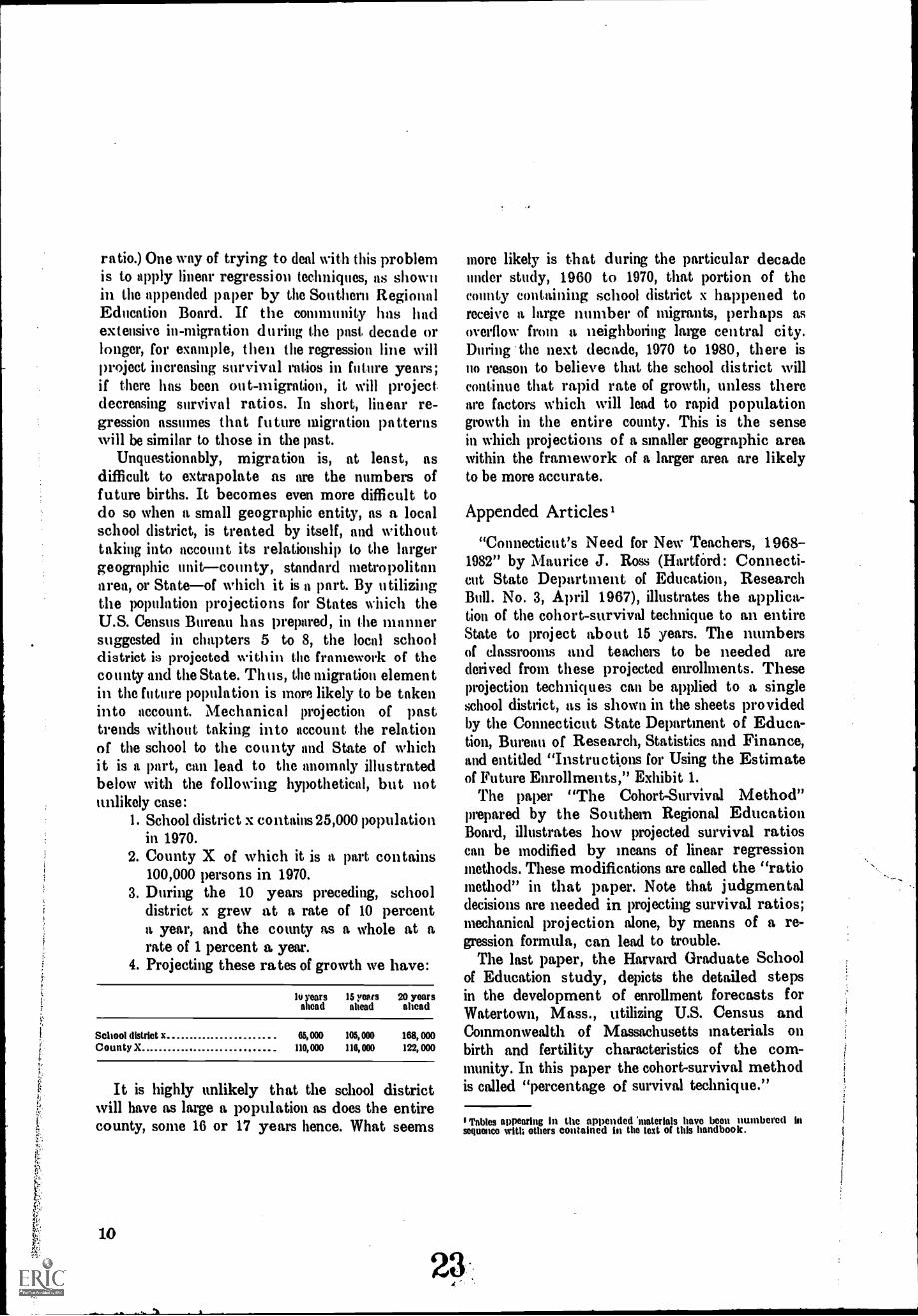
ratio.) One way of trying to deal with this problemis to apply linear regression techniques, as shownin the appended paper by the Southern RegionalEducation Board. If the community has hadextensive in-migration during the past decade orlonger, for example, then the regression line willproject increasing survival ratios in future years;if there has been out-migration, it will projectdecreasing survival ratios. In short, linear re-gression assumes that future migration patternswill be similar to those in the past.
Unquestionably, migration is, at least, asdifficult to extrapolate as are the numbers offuture births. It becomes even more difficult todo so when a small geographic entity, as a localschool district, is treated by itself, and withouttaking into account its relationship to the largergeographic unitcounty, standard metropolitanarea, or Stateof which it is a part. By utilizingthe population projections for States which theU.S. Census Bureau has prepared, in the mannersuggested in chapters 5 to 8, the local schooldistrict is projected within the framework of thecounty and the State. Thus, the migration elementin the future population is more likely to be takeninto account. Mechanical projection of pasttrends without taking into account the relationof the school to the county and State of whichit is a part, can lead to the anomaly illustratedbelow with the following hypothetical, but notunlikely case:
I. School district x contains 25,000 populationin 1970.
2. County X of which it is a part contains100,000 persons in 1970.
3. During the 10 years preceding, schooldistrict x grew at a rate of 10 percenta year, and the county as a whole at arate of 1 percent a year.
4. Projecting these rates of growth we have:
lu years 15 yesesahead ahead
20 yearsahead
School district x 65,000 105,000 168, 000County X 110,000 116, 000 122, 000
It is highly unlikely that the school districtwill have as large a population as does the entirecounty, some 16 or 17 years hence. What seems
10
more likely is that during the particular decadeunder study, 1960 to 1970, that portion of thecounty containing school district x happened toreceive a large number of migrants, perhaps asoverflow front a neighboming large central city.During the next decade, 1970 to 1980, there isno reason to believe that the school district willcontinue that rapid rate of growth, unless thereare factors which will lead to rapid populationgrowth in the entire county. This is the sensein which projections of a smaller geographic areawithin the framework of a larger area are likelyto be more accurate.
Appended Articles'
"Connecticut's Need for New Teachers, 1968-1982" by Maurice J. Ross (Hartford: Connecti-cut State Department of Education, ResearchBull. No. 3, April 1967), illustrates the applica-tion of the cohort-survival technique to an entireState to project about 15 years. The numbersof classroom and teachers to be needed arederived from these projected enrollments. Theseprojection techniques can be applied to a singleschool district, as is shown in the sheets providedby the Connecticut State Department of Educa-tion, Bureau of Research, Statistics and Finance,and entitled "Instructions for Using the Estimateof Future Enrollments," Exhibit 1.
The paper "The Cohort-Survival Method"prepared by the Southern Regional EducationBoard, illustrates how projected survival ratioscan be modified by means of linear regressionmethods. These modifications are called the "ratiomethod" in that paper. Note that judgmentaldecisions are needed in projecting survival ratios;mechanical projection alone, by means of a re-gression formula, can lead to trouble.
The last paper, the Harvard Graduate Schoolof Education study, depicts the detailed stepsin the development of enrollment forecasts forWatertown, Mass., utilizing U.S. Census andCommonwealth of Massachusetts materials onbirth and fertility characteristics of the com-munity. In this paper the cohort-survival methodis called "percentage of survival technique."
I Tables appearing in the appended 'materials have been numbered insequence with others contained in the text of this handbook.
Page
D-15. Estimates of population, adults 16 and over not enrolled ingrades 1-12, and senior class enrollments, by county region,1960 to 1980 by 5-year intervals_ 103
D-16. Estimates of population, adults 16 and over and not enrolled in
grades 1-12, and senior class enrollments, by school district,1960-80, by 5-year intervals 103
D-17. Age distributions, Bucks County, 1950, 1960, 1970, 1980 105
D-18. Dwelling units, 1950, 1960 and as authorized, 1960-67, Bucks
County 105
D-19. Approved lotsBucks County Planning Commission final re-view, 1960-66. 105
E-1. Total State and county shares of fall public school enrollment,State of Maryland, 1956-66, grades 1 to 4 106
E-2. Total State and county shares of fall public school enrollment,State of Maryland, 1956-66, grades 5 to 8 107
E-3. Total State and county shares of fall public school enrollment,State of Maryland, 1956-66, grades 9 to 12 107
E-4. Shares of total public school fall enrollment, for California Sta-tistical Areas, 1947-66, grades 1 to 4 108
E-5. Shares of total public school fall enrollment, for California Sta-tistical Areas, 1947-66, grades 5 to 8 108
E-6. Share3 of total public school fall enrollment, for CaliforniaStatistical Areas, 1947-66, grades 9 to 12 108
E-7. Trend equations for county shares, State of Maryland, 1957 to1962
109
E-8. Unadjusted sums of local area projected school enrollmentshares, States of Maryland and California, 1965 and 1980_ _ _ 109
E-9. Trend equations for county shares, State of Maryland, 1956 to1966
109
E-10. State of California, 1965, comparison of actual and projections,parts I, II, and III 111
E-11. Exponential smoothing trend equations for Statistical Areashares of total State enrollment, State of California, period1947-1960
112
E-12. Actual and projected enrollment by State Statistical Area, Stateof California, 1965, by 4-4-4 organization 113
E-13. Summary comparisons of projected and observed shares andenrollment by grade groups and Statistical Areas, California,
1965113
E-14. Exponential smoothing trend equations for Statistical Areashares of total State enrollment, and 1980 projected shares,State of California, data period 1947-66 114
E-15. Variation among grade groups, projected 1980 shares, State of
California, 0.500 smoothing constant 114
F-1. Shares of total State enrollment, demographic and economiccharacteristics, Calvert County, Md., 1956 to 1965 117
F-2. Cohort ratios of shares of total State enrollment, demographic
and economic characteristics, Calvert County, Md., 1956 to1965
117
F-3. Partial regression and correlation coefficients, Calvert County,Md., grades 1 to 4, 1956 to 1962 117
CONNECTICUT'S NEED FOR NEW TEACHERS 1968-82
By Maurice J. Ross, ChiefBureau of Research, Statistics and Finance
(Table numbers ours)
IntroductionEnrollments in the public schools, including the endowed
and incorporated academies of Connecticut, have beenincreasing and they will continue to increase during tlu .
next decade. Indications are, however, that the increaseswill be quite modest compared to increases in the pastdecade. If Connecticut can solve the problems involved
in matching the numbers of new teachers needed to theareas of subjects in which they are needed, the perennialteacher shortage may at long last be alleviated, at leasttemporarily. However, the introduction of more "headstart" pupils and more kindergarten pupils may well in-
crease the number of teachers needed. Other educationalchanges are operating to reduce the ratio of children toteachers and so increase the demand for teachers. We need
more experience before we can make estimates which takethese changes into account. Meanwhile, the projectedteacher needs may be considered as minimal.
This report is the 1967 revision of the study of teacherneeds. More recent information on births and enrollmentsin Connecticut schools have been used in this revision.Estimated enrollments are different from those in theprevious reports. Actual births have varied from what wasexpected and estimated births have been revised. Thepercentage of children attending kindergarten is increasing.Public school enrollments, including special classes, passed500,000 in 1961-62; they will ixtss 620,000 in 1969 and
700,000 by 1980.These predictions are more accurate for the earlier
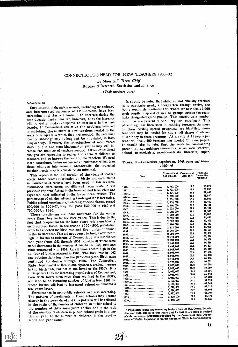
years than they are for the later years. This is due to thefact that projections for the later years rely more heavilyon predicted births. In the decade 1950-1960, populationexperts expected the birth rate and the number of annualbirths to decrease. This did not occur; in fact, a new recordhigh in births to residents of Connecticut was establishedeach year from 1952 through 1957. (Table 3) There weresmall decreases in the number of births in 1958, 1959 and1960 compared with 1957. An all time record high in thenumber of births occurred in 1961. The birth rate in 1962
was substantially less than the previous year. Birth ratescontinued to decline through 1966. The ConnecticutState Department of Health anticipates a gradual increasein the birth rate, but not to the level of the 1950's. It isanticipated that the increasing population of Connecticut,even with lower birth rates than we had in the 1950's,will lead to an increasing number of births from 1967 on.These births will lead to increased school enrollments afew years later.
Enrollments in non-public schools are also increasing.The pattern of enrollments in these schools may becomeclearer in the years ahead and this pattern will be reflectedin the ratio of the number of children in public school tothe number of births some years earlier and in the ratioof the number of children in public school grade in a par-ticular year to the number of children in the previousgrade one year earlier.
24
It should be noted that children not officially enrolledin a particular grade, kindergarten through twelve, arebeing separately accounted for. There arc now about 6,000such pupils in special classes or groups outside the regu-larly designated grade groups. This constitutes a numberecptal to one percent of the "regular" enrollment.. Thispercentage has been used in making forecasts. As morechildren needing special programs are identified, moreteachers may be needed for the small classes which arecustomary in these programs. At a ratio of 15 pupils perteacher, about 400 teachers are needed for these pupils.It should also be noted that the needs for non-teachingpersonnel, e.g., guidance counselors, school social workers,school psychologists, psychometrists, librarians, super-
TAntal 3.Connecticut populat ion, birth rates and births,1940-76
YearConnecticut Connecticutpopulation I birth rate
Births toConnecticutresidents
1940. 1, 712, 000 14. 0 25, 074
1041 1, 761, 000 10.5 28, 996
1942 1, 824, 000 20.3 37,059
1043 1, 869, 000 20.8 38, 880
1044. 1, 804, 000 17. 9 33. 986
1045 1, 905, 000 17. 5 33, 409
1940. 1, 916, 000 21.5 41,131
1047 1, 932, 000 23.4 45, 181
1948 1, 048, 000 21. 5 41, 965
1049. 1, 980, 000 20.0 40, 819
1950 2, 016, 000 20.1 40, 485
1051 2, 052, 000 21. 2 43, 506
1952 2, 106, 000 22.1 46, 537
1953. 2, 173, 000 22.1 47, 996
1954. 2, 246, 000 22.5 50, 428
1955 2, 298, 000 22.8 52, 339
1956 2, 342, 000 22.9 53, 684
1957. 2, 393, 000 23.8 56, 909
1958 2, 456, 000 22.9 56, 244
1959 2, 498, 000 22.0 56, 423
1960 2, 844, 000 22.3 56, 659
1961. 2, 604, 000 21.9 57, 046
1962 2, 063, 000 20.8 55, 480
1963 2, 711, 000 20.8 56, 476
1984 2, 775, 000 20.4 56, 611
1965. 2, 825, 000 19.2 54, 208
1986 2, 873, 000 18.2 52, 289
1967. 2, 929, 000 18.4 53, 894
1068. 2, 986, 000 18.0 55, 540
1969 3, 043, 000 18.8 57, 208
1970. 3, 100, 000 19.1 59, 210
1071 3, 158, 000 19.3 60,949
1972 3, 216, 000 19.5 62, 712
1973 3, 274, 000 19.7 64, 498
1974 3, 332, 000 19.9 66, 307
1975 3, 390, 000 20.2 68, 478
1976 3, 448, 000 20.2 69, 650
I Population figures for years ending in 0 are from tho U.S. Census. Popula-tion and birth data for interim years and for 1966 on aro based on revised
calculations and/or predictions supplied by the Connecticut State Depart-
ment of Health. Population to nearest thousand. Births to nearest hundred.
11
Page
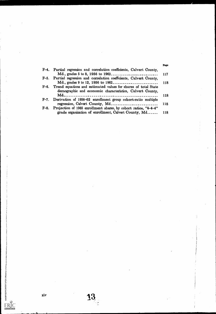
F-4. Partial regression and correlation coefficients, Calvert County,Md., grades 5 to 8, 1956 to 1962 117
F-5. Partial regression and correlation coefficients, Calvert County,Md., grades 9 to 12, 1956 to 1962 118
F-6. Trend equations and estimated values for shares of total Statedemographic and economic characteristics, Calvert County,Md 118
F-7. Derivation of 1956-62 enrollment group cohort-ratio multipleregression, Calvert County, Md 118
F-8. Projection of 1965 enrollment shares, by cohort ratios, "4-4-4"grade organization of enrollment, Calvert County, Md 118
xiv
visors and administrators, are not taken into account inthis bulletin.
It is suggested that the data in this bulletin be carefullystudied by citizens and school personnel of Connecticut.It is believed that a knowledge of the facts herein pre-sented will alert the State of Connecticut to the need forfinding satisfactory solutions to the problems of teachereducation and placement.
Projections should not be considered exact predictions;predictions cannot be accurate to the last digit. A reason-able allowance for error is five percent either way.
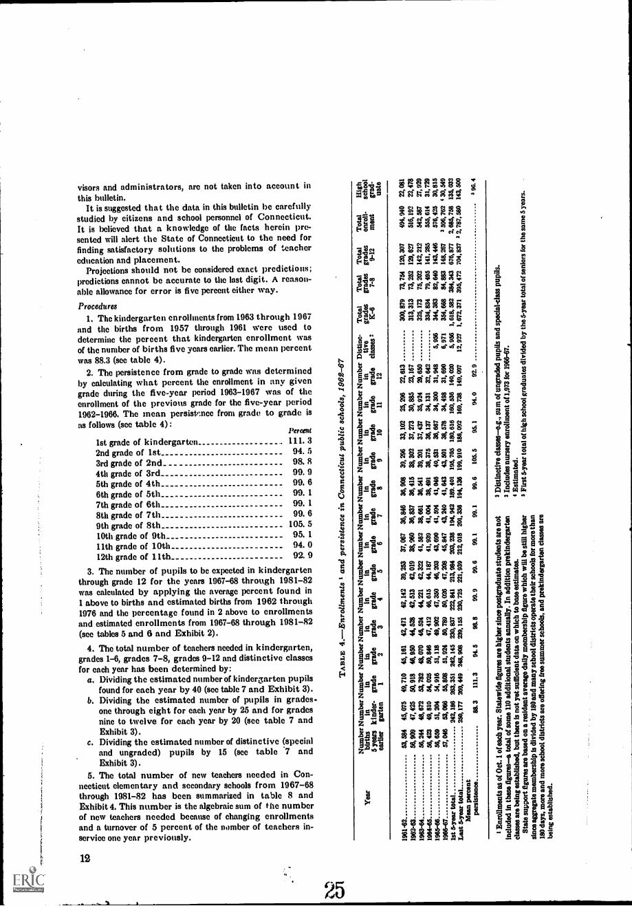
Procedures1. The kindergarten enrollments from 1963 through 1967
and the births from 1957 through 1961 were used todetermine the percent that kindergarten enrollment wasof the number of births five years earlier. The mean percentwas 88.3 (sec table 4).
2. The persistence from grade to grade was determinedby calculating what percent the enrollment in any givengrade during the five-year period 1963-1967 was of theenrollment of the previous grade for the five-year period1962-1966. The mean persisinnce from grade to grade isas follows (see table 4):
Percent
1st grade of k i n dergar ten III. 32nd grade of 1st 94. 53rd grade of 2nd 98. 84th grade of 3rd 99. 95th grade of 4th 99. 66th grade of 5th 99. 17th grade of 6th 99. 18th grade of 7th 99. 69th grade of 8th 105. 510th grade of 9th 95. 111th grade of 10th 94. 012th grade of 11th 92. 9
3. The number of pupils to be expected in kindergartenthrough grade 12 for the years 1967-68 through 1981-82was calculated by applying the average percent found in1 above to births and estimated births from 1962 through1976 and the percentage found in 2 above to enrollmentsand estimated enrollments from 1967-68 through 1981-82(see tables 5 and 6 and Exhibit 2).
4. The total number of teachers needed in kindergarten,grades 1-6, grades 7-8, grades 9-12 and distinctive classesfor each year has been determined by:
a. Dividing the estimated number of kindergarten pupilsfound for each year by 40 (see table 7 and Exhibit 3).
b. Dividing the estimated number of pupils in grades-one through eight for each year by 25 and for gradesnine to twelve for each year by 20 (see table 7 andExhibit 3).
c. Dividing the estimated number of distinctive (specialand ungraded) pupils by 15 (see table 7 andExhibit 3).
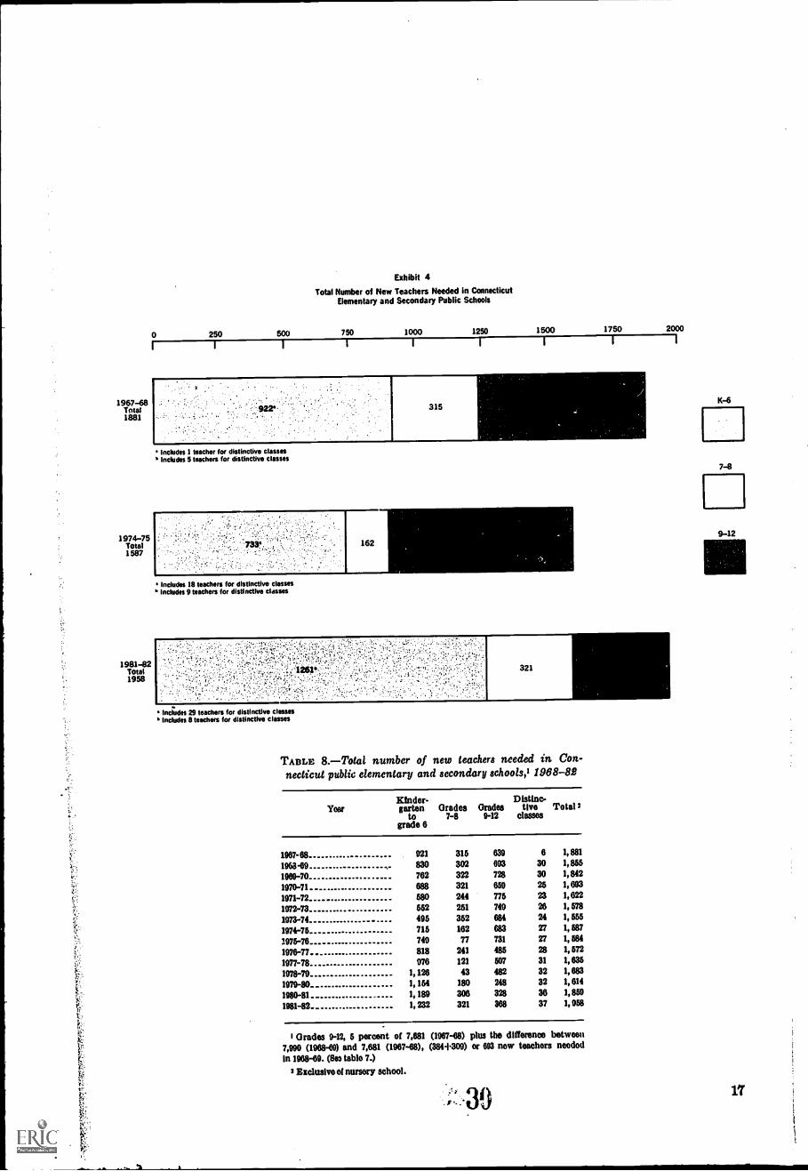
5. The total number of new teachers needed in Con-necticut elementary and secondary schools from 1967-68through 1981-82 has been summarized in table 8 andExhibit 4. This number is the algebraic sum of the numberof new teachers needed because of changing enrollmentsand a turnover of 5 percent of the number of teachers in-service one year previously.
12
25
aftiu
"eatg?,
-0
412
-ssv,gab,
6SkTiAZg 0E=Vf..1zg 0Z "4
".
z t4 0
Zg
°
°
Pits
°
!SID0
0
ar'
acq
is a-
.g S
0511zm1Ngu
giftidggglw--
§EMIRFAaor
vg.Miknge174erig
4NEUIREp-gf.leattg
EMRINEM6146,5
.femior
lalS11§§ggggeiggg
AgEEIMgggggggg
REWiEEEgggggggg
MENU§geggf4gg
UZI-JAM§ggggq:.711,
ggg.1.1rogg
gg.1.1411u
mmi§al444.122flil§i0
$11U1W.iqjg/gf!EF14t4gedgg
fgagggig
MgliM14itcsrdgg
ifieS1dgisfgaf
Si
0
e:
II 11§
a12Be=mu(00.2-.4oEeclitegco 21
g28"I1.4101
142112.0a4a8
Ns g 4V§all2M1=47
I g ;
.0E41-
Vtaliampt;
igslim' A
AVo 4214g galitariC
§.32241.2"1314gi1 0ca roe-10m-12.1"
CHAPTER 1
INTRODUCTION
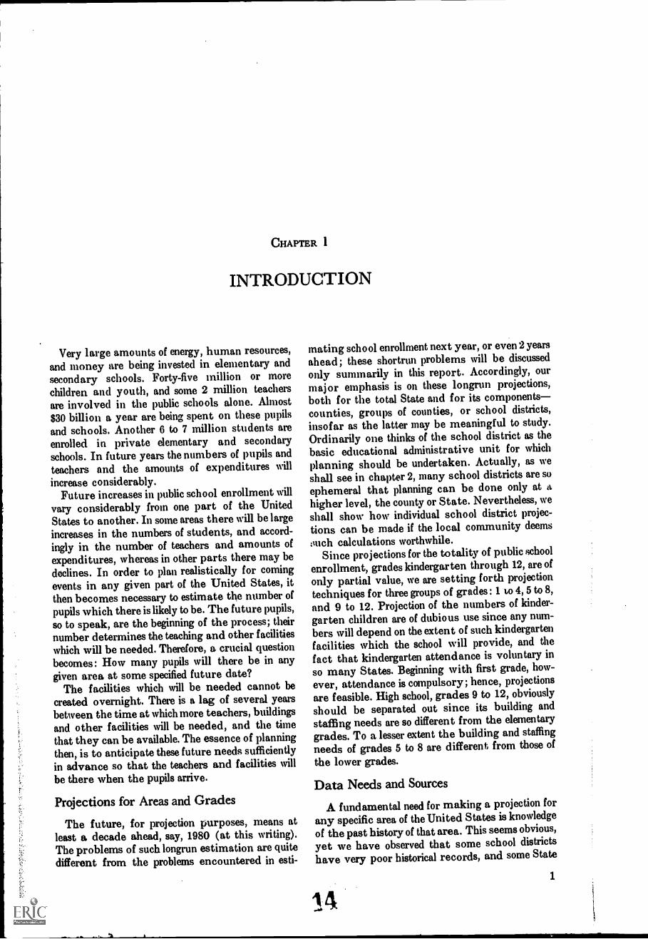
Very large amounts of energy, human resources,and money are being invested in elementary andsecondary schools. Forty-five million or morechildren and youth, and some 2 million teachers
are involved in the public schools alone. Almost$30 billion a year are being spent on these pupilsand schools. Another 6 to 7 million students areenrolled in private elementary and secondaryschools. In future years the numbers of pupils andteachers and the amounts of expenditures willincrease considerably.
Future increases in public school enrollment will
vary considerably from one part of the UnitedStates to another. In some areas there will be largeincreases in the numbers of students, and accord-ingly in the number of teachers and amounts of
expenditures, whereas in other parts there may bedeclines. In order to plan realistically for comingevents in any given part of the United States, itthen becomes necessary to estimate the number ofpupils which there is likely to be. The future pupils,so to speak, are the beginning of the process; theirnumber determines the teaching and other facilities
which will be needed. Therefore, a crucial questionbecomes: How many pupils will there be in anygiven area at some specified future date?
The facilities which will be needed cannot becreated overnight. There is a lag of several yearsbetween the time at which more teachers, buildingsand other facilities will be needed, and the timethat they can be available. The essence of planningthen, is to anticipate these future needs sufficientlyin advance so that the teachers and facilities willbe there when the pupils arrive.
Projections for Areas and Grades
The future, for projection purposes, means atleast a decade ahead, say, 1980 (at this writing).The problems of such longrun estimation are quitedifferent from the problems encountered in esti-
mating school enrollment next year, or even 2 years
ahead; these shortrun problems will be discussedonly summarily in this report. Accordingly, ourmajor emphasis is on these longrun projections,both for the total State and for its componentsco u n ti es, groups of coup ties, or school districts,insofar as the latter may be meaningful to study.Ordinarily one thinks of the school district as thebasic educational administrative unit for whichplanning should be undertaken. Actually, as weshall see in chapter 2, many school districts are soephemeral that planning can be done only athigher level, the county or State. Nevertheless, we
shall show how individual school district projec-tions can be made if the local community deemstmch calculations worthwhile.
Since projections for the totality of public school
enrollment, grades kindergarten through 12, are ofonly partial value, we are setting forth projectiontechniques for three groups of grades : 1 up 4, 5 to 8,
and 9 to 12. Projection of the numbers of kinder-garten children are of dubious use since any num-bers will depend on the extent of such kindergartenfacilities which the school will provide, and thefact that kindergarten attendance is voluntary inso many States. Beginning with first grade, how-
ever, attendance is compulsory; hence, projections
are feasible. High school, grades 9 to 12, obviously
should be separated out since its building andstaffing needs are so different from the elementarygrades. To a lesser extent the building and staffingneeds of grades 5 to 8 are different from those ofthe lower grades.
Data Needs and Sources
A fundamental need for making a projection forany specific area of the United States is knowledge
of the past history of that area. This seems obvious,
yet we have observed that some school districtshave very poor historical records, and some State
1
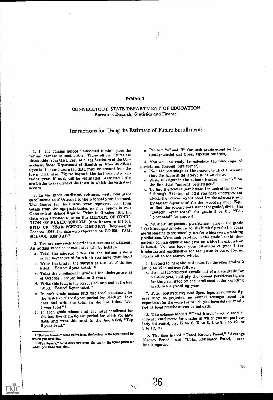
Exhibit 1
CONNECTICUT STATE DEPARTMENT OF EDUCATIONBureau of Research, Statistics and Finance
Instructions for Using the Estimate of Future Enrollments
1. In the column headed "allocated births" place theannual number of such births. These official figures areobtainable from the Bureau of Vital Statistics of the Con-necticut State Department of Health or from its officialreports. In most towns the data may be secured from thetown clerk also. Figures beyond the last completed cal-endar year, if used, will be estimated'. Allocated birthsare births to residents of the town in which the birth itselfoccurs.
2. In the grade enrollment columns, write your gradeenrollments as of October 1 of the 6 school years indicated.The figures for the current year represent your town
totals from the age-grade tables as they appear in yourConnecticut School Register. Prior to October 1966, thedata were reported to us on the REPORT OF CONDI-TION OF PUBLIC SCHOOLS (now known as ED 001,END OF YEAR SCHOOL REPORT). Beginning inOctober 1966, the data were reported on ED 006, "FALL
SCHOOL REPORT."
3. You arc now ready to perform a number of additions.An adding machine or calculator will be helPful.
a. Total the allocated births for the bottom 5 yearsin the 6-year period for which you have exact data.'
b. Write the total in the margin at the left of the linetitled, "Bottom 5-year total." 2
c. Total the enrollment in grade 1 (or kindergarten) asof October 1 for/the bottom 5 years.
d. Write this totapn the correct column and in the linetitled, "Bottonl 5-year total."
e. In each grade column find the total enrollment forthe first fivd of the 6-year period for which you havedata and write this total in the line titled, "Top5-year total." 2
f. In each grade column find the total enrollment forthe last five of the 6-year period for which you havedata and write this total in the line titled, "Top
5-year total."
"Bottom 15-yeara," count up five from the bottom in the 6-year period for
which you have data.2 "Top &years," count down five from the top in the 6-year period for
which you have exact data.
g. Perform "e" and "1" for each grade except for P.C.(postgraduate) and Spec. (special students).
4. You are now ready to calculate the percentage ofpersisteneo (percent persistence).
a. Find the percentage to the nearest tenth of 1 percentthat the figure in 3d above is of 3b above.
b. Write this figure in the column headed "I" or "k" onthe line titled "percent persistence."
c. To find the percent persistence for each of the grades2 through 12 (1 through 12 if you have kindergartens)divide the bottom 5-ycar total for the selected gradeby the top 5-year total for the nreceding grade. E.g.,to find the percent persistence for grade 5, divide the"Bottom 5-year total" for grade 5 by the "Top5-y ear total" for grade 4.
5. Multiply the percent persistence figure in the grade(or kindergarten) column by the birth figure for the years
corresponding to the school years for whieh you arc makingpredictions. Write each product in the grade 1 (or kinder-garten) column opposite the year on whbh the calculationis based. You now have your estimates of grade 1 (orkindergarten) enrollments for the years to come. Roundfigures off to the nearest whole.
6. Proceed to make the estimates for the other grades 2(or 1) to 12 in order as follows:
a. To find the predicted enrollment of a given grade fora future year, multiply the percent persistence figurefor the given grade by the enrollment in the precedinggrade in the preceding year.
7. P. G. (postgraduate) and Spec. (special students) fig-ures may be projected as annual averages based onexperience for the years for which you have data or modi-fied as local practice seems to indicate.
8. The columns headed "Total Enrol." may be used toindicate enrollments for grades in which you are particu-larly interested, e.g., K to 6, K to 8, 1 to 8, 7 to 12, or9 to 12, etc.
9. The iines headed "Total Known Period," "AverageKnown Period," and "Total Estimated Period," maybe disregarded.
13
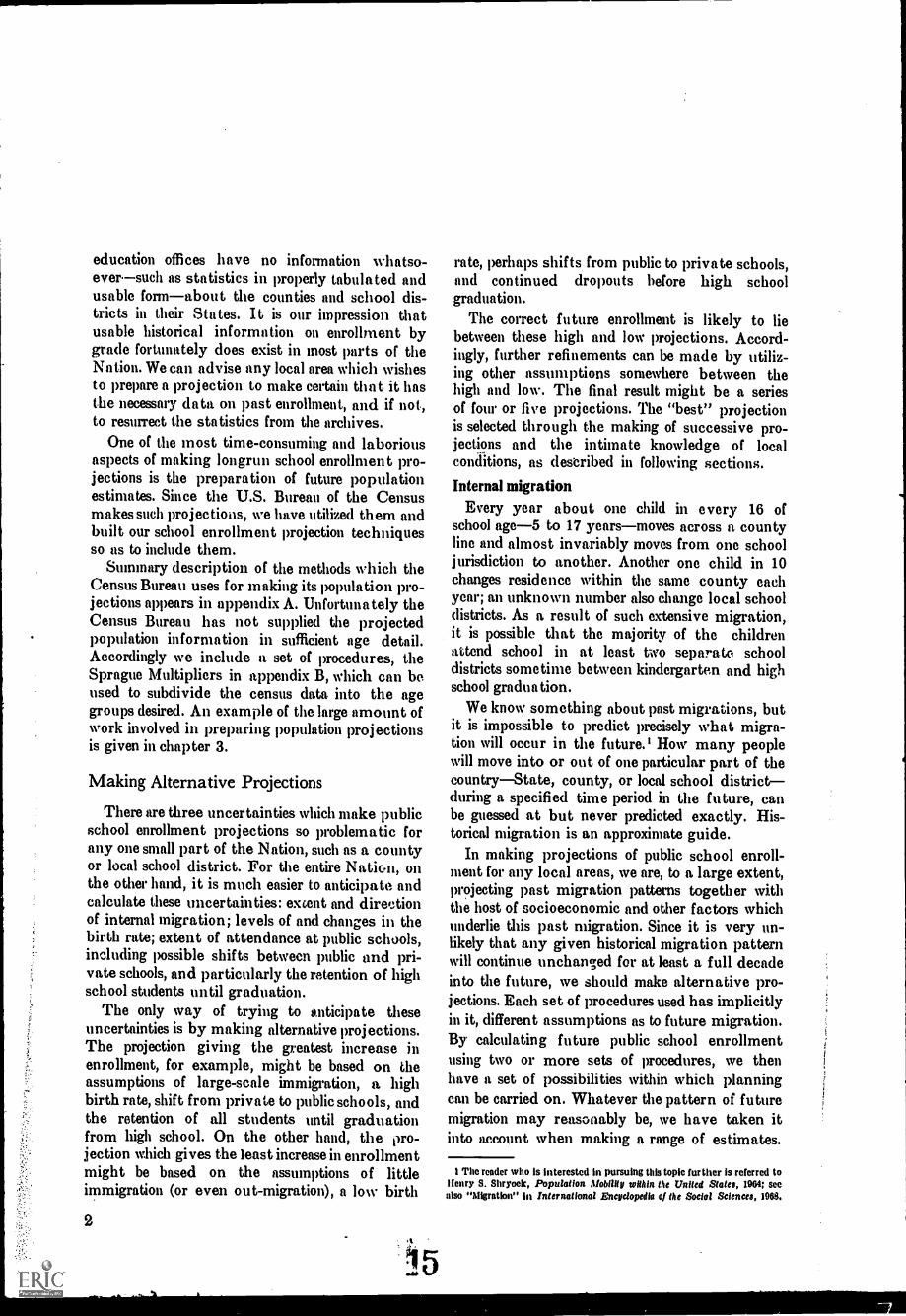
education offices have no information whatso-eversuch as statistics in properly tabulated andusable formabout the counties and school dis-tricts in their States. It is our impression thatusable historical information on enrollment bygrade fortunately does exist in most parts of theNation. We can advise any local area which wishesto prepare a projection to make certain that it hasthe necessary data on past enrollment, and if not,to resurrect the statistics from the archives.
One of the most time-consuming and laboriousaspects of making longrun school enrollment pro-jections is the preparation of future populationestimates. Since the U.S. Bureau of the Censusmakes such projections, we have utilized them andbuilt our school enrollment projection techniquesso as to include them.
Summary description of the methods which theCensus Bureau uses for making its population pro-jections appears in appendix A. Unfortunately theCensus Bureau has not supplied the projectedpopulation information in sufficient age detail.Accordingly we include a set of procedures, theSprague Multipliers in appendix B, which can beused to subdivide the census data into the agegroups desired. An example of the large amount ofwork involved in preparing population projectionsis given in chapter 3.
Making Alternative Projections
There are three uncertainties which make publicschool enrollment projections so problematic forany one small part of the Nation, such as a countyor local school district. For the entire Nation, onthe other hand, it is much easier to anticipate andcalculate these uncertainties: extent and directionof internal migration; levels of and changes in thebirth rate; extent of attendance at public schools,including possible shifts between public and pri-vate schools, and particularly the retention of highschool students until graduation.
The only way of trying to anticipate theseuncertainties is by making alternative projections.The projection giving the greatest increase inenrollment, for example, might be based on theassumptions of large-scale immigration, a highbirth rate, shift from private to public schools, andthe retention of all students until graduationfrom high school. On the other hand, the pro-jection which gives the least increase in enrollmentmight be based on the assumptions of littleimmigration (or even out-migration), a low birth
2
1 5
rate, perhaps shifts from public to private schools,and continued dropouts before high schoolgraduation.
The correct future enrollment is likely to liebetween these high and low projections. Accord-ingly, further refinements can be made by utiliz-ing other assumptions somewhere between thehigh and low. The final result might be a seriesof four or five projections. The "best" projectionis selected through the making of successive pro-jections and the intimate knowledge of localconditions, as described in following sections.
Internal migrationEvery year about one child in every 16 of
school age-5 to 17 yearsmoves across a countyline and almost invariably moves from one schooljurisdiction to another. Another one child in 10changes residence within the same county eachyear; an unknown number also change local schooldistricts. As a result of such extensive migration,it is possible that the majority of the childrenattend school in at least two separate schooldistricts sometime between kindergarten and highschool gradua tion.
We know something about past migrations, butit is impossible to predict precisely what migra-tion will occur in the future.' How many peoplewill move into or out of one particular part of thecountryState, county, or local school districtduring a specified time period in the future, canbe guessed at but never predicted exactly. His-torical migration is an approximate guide.
In making projections of public school enroll-ment for any local areas, we are, to a large extent,projecting past migration patterns together withthe host of socioeconomic and other factors whichunderlie this past migration. Since it is very un-likely that any given historical migration patternwill continue unchanged for at least a full decadeinto the future, we should make alternative pro-jections. Each set of procedures used has implicitlyin it, different assumptions as to future migration.By calculating future public school enrollmentusing two or more sets of procedures, we thenhave a set of possibilities within which planningcan be carried on. Whatever the pattern of futuremigration may reasonably be, we have taken itinto account when making a range of estimates.
1 The reader who is interested in pursuing this topic further is referred toHenry S. Shryoek, Population Mobility within the United States, 1964; secalso "Migration" in International Encyclopedia of the Social Sciences, 1968.
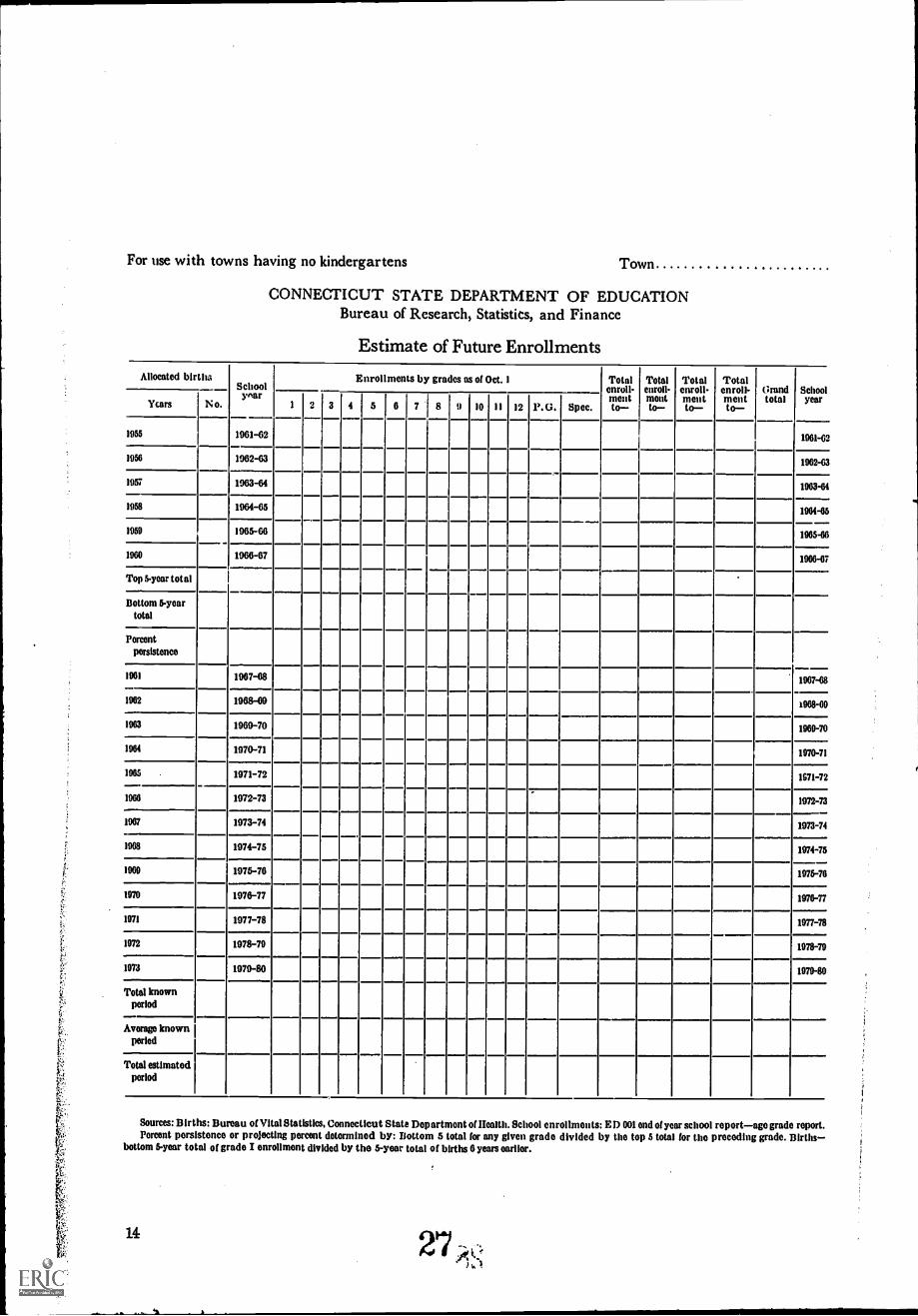
For use with towns having no kindergartens Town
CONNECTICUT STATE DEPARTMENT OF EDUCATIONBureau of Research, Statistics, and Finance
Estimate of Future Enrollments
Allocated birthsS choolynar
Enrollments by grades as of Oct. 1 Totalenroll-mentto
Totalenroll-moatto
Totalenroll-m en tto
Totalenroll-m cutto-
Grandtotal
SchoolyearYcars No. 1 2 3 4 5 6 7 8 9 10 I I 12 P. G. Spec.
1955 1961-62 1061-62
1956 1962-63 1962-63
1957 1963-64 1963-64
1958 1964-65 1904-65
1959 1965-66 1965-66
1960 1966-67 1966-67
Top 5-yoar total -
Bottom 5-yoartotal
Percentpersistence
1961 1967-68 1967-68
1962 1968-69 1968-09
1963 1969-70 1969-70
1964 1970-71 1970-71
1005 1971-72 1671-72
1966 1972-73 1972-73
1967 1973-74 1973-74
1968 1974-75 1974-75
1969 1975-76 1975-76
1970 1976-77 1976-77
1971 1977-78 1977-78
1972 1978-79 1978-79
1973 1979-80 1979-80
Total knownperiod
Avorago knownperiod
Total estimatedperiod
Sources: Births: Bureau of Vital Statistics, Connecticut State Dopartmont of Health. School enrollments: ED 001 and of year school roportago grado report.Percent persistence or projecting porcont determined by: Bottom 5 total for any given grado divided by tho top 5 total for tho preceding grade. Births
bottom 5-yoar total of grade I onrollmont divided by the 5-year total of births 6 years earlier.
14
.10
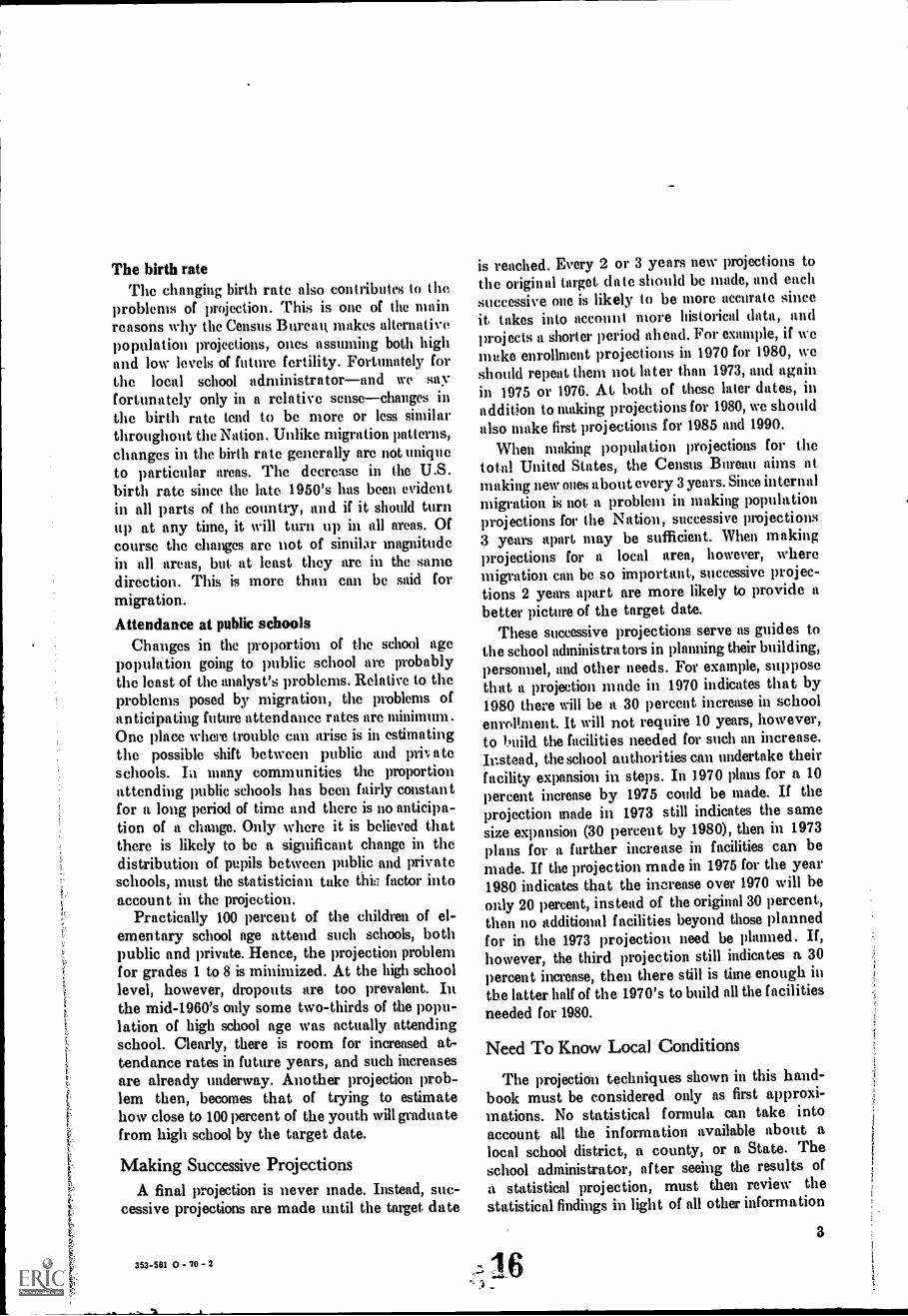
The birth rateThe changing birth rate also contributes to the
problems of projection. This is one of the mainreasons why the Census Bureau, makes alternativepopulation projections, ones assuming both highand low levels of future fertility. Fortunately forthe local school administratorand we sayfortunately only in a relative sensechanges inthe birth rate tend to be more or less similarthroughout the Nation. Unlike migration patterns,changes in the birth rate generally are not uniqueto particular areas. The decrease in the U.S.birth rate since the late 1950's has been evidentin all parts of the country, and if it should turnup at any time, it will turn up in all areas. Ofcourse the changes are not of similar magnitudein all areas, but at least they are in the samedirection. This is more than can be said formigration.
Attendance at public schoolsChanges in the proportion of the school age
population going to public school are probablythe least of the analyst's problems. Relative to theproblems posed by migration, the problems ofanticipating future attendance rates are minimum.One place where trouble can arise is in estimatingthe possible shift between public and priv ateschools. In many communities the proportionattending public schools has been fairly constantfor a long period of time and there is no anticipa-tion of a change. Only where it is believed thatthere is likely to be a significant change in thedistribution of pupils between public and privateschools, must the statistician take thif: factor intoaccount in the projection.
Practically 100 percent of the children of el-ementary school age attend such schools, bothpublic and private. Hence, the projection problemfor grades 1 to 8 is minimized. At the high schoollevel, however, dropouts are too prevalent. Inthe mid-1960's only some two-thirds of the popu-lation of high school age was actually attendingschool. Clearly, there is room for increased at-tendance rates in future years, and such increasesare already underway. Another projection prob-lem then, becomes that of trying to estimatehow close to 100 percent of the youth will graduatefrom high school by the target date.
Making Successive ProjectionsA final projection is never made. Instead, suc-
cessive projections are made until the target date
353-581 0 - 70 - 2
is reached. Every 2 or 3 years new projections tothe original target date should be made, and eachsuccessive one is likely to be more accurate sinceit takes into account more historical data, andprojects a shorter period ahead. For example, if wemake enrollment projections in 1970 for 1980, weshould repeat them not later than 1973, and againin 1975 or 1976. At both of these later dates, inaddition to making projections for 1980, we shouldalso make first projections for 1985 and 1990.
When making population projections for thetotal United States, the Census Bureau aims atmaking new ones about every 3 years. Since internalmigration is not a problem in making populationprojections for the Nation, successive projections3 years apart may be sufficient. When makingprojections for a local area, however, wheremigration can be so important, successive projec-tions 2 years apart are more likely to provide abetter picture of the target date.
These successive projections serve as guides tothe school administrators in planning their building,personnel, and other needs. For example, supposethat a projection made in 1970 indicates that by1980 there will be a 30 percent increase in schoolenrollment. It will not require 10 years, however,to 'mild the facilities needed for such an increase.Instead, the school authorities can undertake theirfacility expansion in steps. In 1970 plans for a 10
percent increase by 1975 could be made. If theprojection made in 1973 still indicates the samesize expansion (30 percent by 1980), then in 1973plans for a farther increase in facilities can be
made. If the projection made in 1975 for the year1980 indicates that the increase over 1970 will beonly 20 percent, instead of the original 30 percent,then no additional facilities beyond those plannedfor in the 1973 projection need be planned. If,however, the third projection still indicates a 30percent increase, then there still is time enough inthe latter half of the 1970's to build all the facilitiesneeded for 1980.
Need To Know Local Conditions
The projection techniques shown in this hand-book must be considered only as first approxi-mations. No statistical formula can take intoaccount all the information available about alocal school district, a county, or a State. Theschool administrator, after seeing the results ofa statistical projection, must then review thestatistical findings in light of all other information
- 6
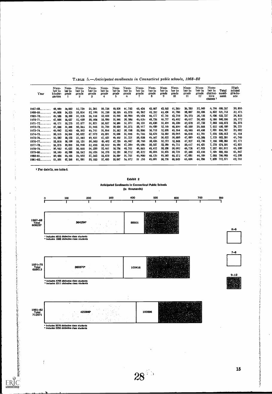
TABLE 5.-Anticipalcd enrollments in Connecticut public schools, 1968-82
Num- Num- Num- Nmn- Num- Num- Num- Num- Num- Num- Num- Num- Num- Nnm- Highber in her in ber in ber in ber in her in her hi her in her in ber hi her in ber in ber in her hi Total school
Year kinder- grade grade grade grade grade grade grade grade grade grade grade grade distinc- enroll- gradu-garten 1 2 3 4 5 6 7 8 0 10 II 12 tive ment ate
classes I
1967-68 98, 980 59, 062 52, 739 51, 301 50, 738 99, 826 4C., 783 45. 434 93, 007 93, 933 41, 369
1068-69 99, 868 54,525 55, 819 52, 106 51, 250 50, 535 99, 378 46, 362 45, 252 45,4311 41, 780
1969-70 99, 988 55, 503 51, 526 55, 199 52, 054 51,045 50, 080 9 8, 939 96, 177 97, 741 43, 210
1970-71 97, 866 65, 637 52, 9 50 50, 908 55, 080 51,846 50, 586 99, 629 98, 738 48,717 95,902
1971-7 0 46, 171 53, 275 62, 577 51, 821 50, 857 54, 869 51, 371; 50, 131 99,430 51,919 40, 330
1972-73 97, 588 51, 388 50, 395 51, 946 51, 760 50, 054 54, 375 50, 917 49, 930 52, 149 48, 899
1973-79 99, 042 52, 965 98, 562 99, 741 51, 894 51,562 50, 108 53, 886 50, 713 52, 676 99, 599
1979-75 50, 515 54, 584 50, 052 47.070 49, 691 51,686 51, 098 49, 796 53, 670 53,502 50,095
10 75-76 52, 22 56, 223 51, 582 99, 9 51 47, 931 99,492 51, 221 50, 638 99, 547 56, 622 50,880
1976-77 53,818 58,190 53, 131 50, 963 49, 902 97,739 99, 09 7 50, 760 50,435 52,272 53, 848
1077-78 55, 375 59,899 54, 090 52, 993 50, 912 99, 291 97, 30!) 9 8, 606 50, 557 53, 209 99, 711
1978-79 56, 952 01, 632 56, 605 54, 330 52, 491 50,708 48, 761 96, 883 98,412 53,338 50, 602
1979-80 58, 549 63, 388 58, 292 55, 926 54, 276 52, 231 50, 252 98, 3 22 96, 995 51, 075 50, 724
1980-81 60, 966 65,165 59, 902 57, 543 55, 870 54, 050 51, 761 99, $00 98, 129 40, 203 98, 572
1981-82 61, 501 67, 299 61, 581 59, 183 57, 985 55, 647 53, 572 51 295 99, 601 50, 770 96, 849
36, 263 3 2, 049 6, 704 608, 257 3 0, 895
38, 887 33, 688 6, 832 621, 713 3 2, 475
39, 273 36, 126 6, 936 633, 737 34, 825
9 0, 617 3 6, 985 6, 986 640,956 3 5, 172
9 2, 678 37, 733 7, 013(1 645, 673 36, 375
93, 550 39, 648 7, 022 (i50, 180 38, 221
9 5, 965 40,458 7, 031 654, 287 3 9, 002
9 6,618 42,701 7, 076 659, 013 41, 169
47,089 43,308 7, 125 663, 391 41,74997, 827 43,740 7, 186 668, 364 92, 171
50, 017 44, 931 7, 278 679, 591 9 2, 831
96, 728 47,023 7, 397 631, 812 95, 330
47, 566 93, 910 7, 509 688, 165 41, 89797, 681 44, 189 7, 668 700, 068 42, 598
95, 658 99, 296 7, 82 712, 571 92, 701
I For detalls, seo table 6
1967-68Total
608257
197,1-75Total
659013
1981-82Total
712571
0 100
Exhibit 2
Anticipated Enrollments in Connecticut Public Schools
(in thousands)
200 300 400 500 600 700 800
Includes 4816 distinctive class studentsIncludes 1888 distinctive class students
Includes 4765 distinctive class students6 Includes 2311 distinctive class students
Includes 5578 distinctive class students6 Includes 2250 distinctive class students
28
K-6
7-8
9-12
15
which he has about his community. The illus-trative projections for 1980 which we show forMaryland (chapter 7) are the first approximationsto 1980. We do not have all the knowledge whichthe State and county educators have. They mustreview the projections and decide for themselveswhether they are probable or not.
At this point the coordination of local schooldistrict projections at the State level becomesimportant. Insofar as the Census Bureau is ableto make usable projections of State populationby age, the enrollment in public schools in theentire State can be projected with a minimum
4
1.1
of error. This means, then, that the sum of thelocal school districts imist equal the State total.If, for example, in the illustrative case of Mary-land, every county board of education shoulddecide that its enrollment will be 10 percentabove that indicated by the statistical projec-tions, some counties will be in deep trouble. Weknow fairly well what the 1980 school enrollmentis likely to be in Maryland. All the counties cannothave 10 percent more than the State. The Statedepartment of education must reconcile suchdiverse adjustments of the original projected1980 figures.
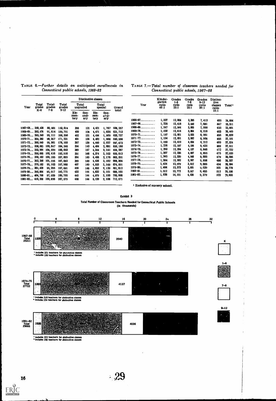
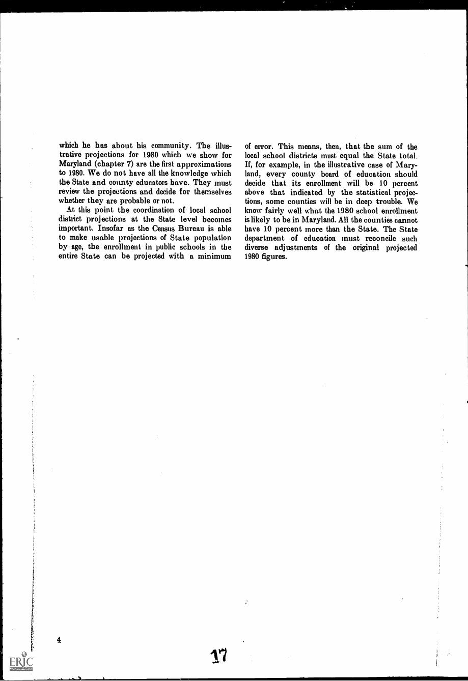
TABLE 6.-Further details on anticipated enrollments in TAntx 7 .-Total number of classroom teachers needed forConnecticut public schools, 1968-82 Connecticut public schools, 1967-82
YearTotal
gradesK-6
Totalgrades
7-8
Totalgrades9-12
Distinctive classes Kinder- Grades Grades7-8
ratio25:1
Grades9-12ratio20:1
Distinc-tive
classesratio15:1
Total Igarten 1-6
Total Total Year ratio ratioungraded special Grand 40:1 25:1
totalEle- Sec- Me- Sec-men- ond. men- on d-tary ary tary nry 1966-67 1,327 12,064 3,395 7, 413 465 24,664
1967-68 I, 225 12,418 3, 540 7, 681 447 28, 311
1967-68._ 359,438 88, 501 153, 614 395 121 4, 421 I, 767 608, 257 1968-69 I, 247 12, 544 3,665 7, 990 455 25,9011968-69._ 363,476 91, 614 159, 791 400 120 4,471 I, 835 621, 713 1969-70 I, 250 12, 614 3,801 8, 318 463 26, 449
1960-70._ 365, 340 95, 111 166, 350 402 131 4,494 I, 909 633, 737 1970-71 I, 197 12, 661 3,935 8, 561 466 26,8201970-71.- 364, 382 98, 367 171, 221 401 135 4, 482 I, 968 640, 956 1971 -70 I, 154 12, 591 3,982 8, 908 466 27, 101
1971-72... 360, 949 99, 561 178, 160 397 139 4,440 2, 027 64f, 673 1972-73 I, 190 12, 419 4, 034 9, 212 469 27,324
1972-73... 358, 065 100, 847 184, 246 394 143 4, 404 2, 081 650, 180 1973-74 I, 226 12, 197 4,184 9, 435 469 27, 511
1973-74... 353,964 104, 599 188, 693 389 147 4,354 2, 141 654, 287 1974-75 I, 263 12, 204 4,137 9, 646 472 27, 722
1974-75._ 355, 605 103, 416 192, 916 391 148 4,374 2, 163 659, 013 1975-76 I, 307 12, 236 4,007 9, 895 475 27, 920
1975-76._ 368,182 100, 185 197, 899 394 149 4,406 2, 176 663,391 1976-77 I, 345 12, 339 4,048 9, 885 479 28, 096
1976-77.- 362, 290 101, 195 197, 693 399 149 4,456 2, 182 668, 364 1977-78 I, 384 12, 592 3,967 9, 898 486 28, 327
1977-78.- 370,182 99, 163 197, 968 407 149 4,553 2, 169 674, 591 1978-79 1, 424 12, 979 3,812 9, 885 494 28, 594
1978-79... 381, 429 95, 295 197, 691 420 146 4, 692 2, 139 681, 812 1979-80 I, 464 13, 373 3,801 9, 639 501 28,778
1979-80.- 392,864 95, 017 192, 775 432 144 4,832 2, 101 688, 165 1980-81 I, 512 13, 772 3,917 9, 485 512 29,198
1980-81.- 404, 766 97, 929 189, 705 445 144 4,979 2, 100 700, 068 1981-82 I, 538 14, 191 4,036 9, 379 522 29,666
1981-82... 416,268 100, 896 187, 579 468 144 5,120 2, 106 712, 571
I Exclusive of nursory school.
Exhibit 3
Total Number of Classroom Teachers Needed for Connecticut Public Schools(in thousands)
0 4 8 12 16 20 2q 28 32
1967-68Total25311
1974-75Total27722
1981-82Total
29666
16
Includes 321 teachers for distinctive classesb Includes 126 teachers for distinctive classes
Includes 318 teachers for distinctive classesIncludes 154 teachers for distinctive classes
Includes 372 teachers for distinctive classesIncludes 150 teachers for distinctive classes
29
1-6
7-8
9-12
f-.;
CHAPTER 2
HOW USEFUL ARE SCHOOL DISTRICTS
AS BASIC UNITS FOR PROJECTION PURPOSES?
The major part of our efforts is devoted tothe presentation of methods for projecting en-rollment for single counties, or groups of con-tiguous counties. Secondary effort will be given tothe methodology of projections for individual
school districts. The reasons for giving firstpriority to counties is that it is much easier tomake reasonable projections for them, whereasthere are a number of factors which make itdifficult to analyze individual school districts.
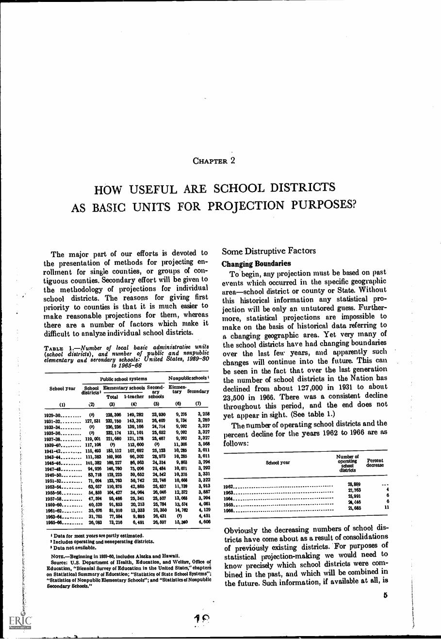
TABLE 1.-Number of local basic administrative units(school districts), and number of _public and nonpublicelementary and secondary schools: United States, 1929-30
to 1965-66
School year
(1)
Public school systems Nonpublic schools
Schooldistricts 2
(2)
Elementary schools Second-ary
schools
(5)
Elemen-tary Secondary
(6) (7)
Total 1-teacher
(3) (4)
1929-30 (3) 238, 306 149, 282 23, 930 0, 275 3, 258
1931-32 127, 531 232, 750 143,391 26,409 9, 734 3, 289
1933-34 (3) 236, 236 139, 166 24, 714 9,992 3, 327
1935-36 (3) 232,174 131, 101 25,652 9, 992 3, 327
1937-38 119, 001 221, 660 121, 178 25, 467 9, 992 3, 327
1939-40 117, 108 (1) 113, 600 (3) 11,306 3, 568
1941-42 115, 493 183, 112 107, 692 25,123 10, 285 3, 011
194344 III, 383 169, 905 96,302 28,973 10, 285 3, 011
1945-46 1U1, 382 160,227 86, 563 24,314 9, 863 3, 294
1947-48 94,926 146, 760 75, 096 25, 484 10,071 3, 292
1949-50 83, 718 128,225 59,652 24, 542 10,375 3,331
1951-52 71,094 123,763 50, 742 23, 748 10,666 3,322
1953-54 63, 057 110, 875 42,865 25,637 11,739 3, 913
1955-56 54, 859 101, 427 34, 964 26,046 12,372 3, 887
1957-58... 47, 594 95,466 25, 341 25, 507 13, 065 3, 994
1959-60 40, 520 91, 853 20, 213 25, 784 13, 574 4, 061
1961-62 35, 676 81,910 13,333 25,350 14, 782 4, 129
1963-64.-- 31, 705 77, 584 9, 895 26, 431 (3) 4, 451
1965-66 26, 983 73, 216 8, 491 26, 597 15, 340 4, 606
Data for most years are partly estimated.2 Includes operating and nonoperating districts.3 Data not available.
NOTE.-Beginning in 1959-60, includes Alaska and Hawaii.Source: U.S. Department of Health, Education, and Welfare, Office of
Education, "Biennial Survey of Education in the United States," chapterson Statistical Summary of Education; "Statistics of State School Systems";"Statistics of Nonpublic Elementary Schools"; and "Statistics of NonpublicSecondary Schools."
P
Some Distruptive FactorsChanging Boundaries
To begin, any projection must be based on pastevents which occurred in the specific geographicarea-school district or county or State. Withoutthis historical information any statistical pro-jection will be only an untutored guess. Further-more, statistical projections are impossible tomake on the basis of historical data referring toa changing geographic area. Yet very many ofthe school districts have had changing boundariesover the last few years, and apparently suchchanges will continue into the future. This canbe seen in the fact that over the last generationthe number of school districts in the Nation hasdeclined from about 127,000 in 1931 to about23,500 in 1966. There was a consistent declinethroughout this period, and the end does notyet appear in sight. (See table 1.)
The number of operating school districts and thepercent decline for the years 1962 to 1966 are asfollows:
School yearNumber ofoperating Percent
school decreasedistricts
1962 28, 859 ...1963
27,763 4
1964.25,991 6
196524,446 8
196621,685 11
Obviously the decreasing numbers of school dis-tricts have come about as a result of consolidationsof previciusly existing districts. *For purposes ofstatistical projection-making we would need toknow precisely which school districts were com-bined in the past, and which will be combined inthe future. Such information, if available at all, is
5
1967-68Total1881
1974-75Total1587
1981-82Total1958
250 500
Exhibit 4
Total Number of New Teachers Needed in ConnecticutElementary and Secondary Public Schools
750 1000 1250 1500 1750 2000
Includes 1 teacher far distinctive classesIncludes 5 teachers for distinctive el
Includes 18 teachers for distinctive classesIncludes 9 teachers for distinctive classes
Incrudes 29 teachers for distinctive classesincludes 8 teachers far distinctive classes
TABLE 8.Total number of new teachers nceded in Con-necticut public elementary and secondary schools,1 1968-82
YearKinder-garten
tograde 6
Grades7-8
Grades9-12
Distinc-tive
classesTotal s
1967-68 921 315 639 6 1, 881
1., 196849 830 302 693 30 1,855
1969-70 762 322 728 30 1,842
1970-71 688 321 659 25 1,693
1971-72 580 244 775 23 1,622
1972-73 552 251 749 28 1, 578
1973-74 495 352 684 24 1, 555
1974-75 715 162 883 27 1,587
; 1975-76 749 77 731 27 1, 584
t1976-77 818 241 486 28 1, 572
1s$,. 1977-78 976 121 507 31 1,635
1978-79 1, 128 43 482 32 1,683
1979-80 1, 164 180 248 32 1,614
1980-8L 1, 189 300 328 36 1,859
1981-82 1,232 321 368 37 1, 958
I Grades 942, 5 percent of 7,681 (1967-68) plus the difference between7,990 (1968-69) and 7,681 (1967-48), (3844-309) or 693 now teachers neededIn 1968-69. (Elea table 7.)
I Exclusive of nursery school.
; 39
K-6
7-8
9-12
17
available only locally. Presumably some historicalrecords are available in State or local offices andcould be used, if all past consolidations were madeby combining whole school districts. But if anyprevious school districts were split and apportionedto other districts, it becomes a very difficult task toreconstruct constant geographic entities.
Of major importance for making statisticalprojections is the fact that future consolidationsare largely unknown at present. In some Statesconsolidations and the redrawing of school bound-aries are in the hands of cou nty or State authoritiesand can be imposed on the school district. In othercases the decision to consolidate or not is made bythe school districts concerned. In either event it isdifficult to predict exactly which school districtboundaries will change, and which will not. Wehazard a guess that ultimately the number of schooldistricts in the United States will approach thenumber of countiesabout 3,000but we have noidea when.
The number of counties in the United Statesand their boundaries have remained largely un-changed for a number of decades, and all ourpresent information strongly suggests that few, ifany, boundary changes are contemplated in theforeseeable future. Accordingly, then, the countyrather than the school district is preferable formaking statistical projections.
Size of School DistrictsAnother statistical problem is that many school
districts (as of fall 1966) were too small to permitmaking reliable projections. The enrollment in aschool district with but a few hundred students, oreven a very few thousand, could vary enormouslyand unpredictably. In general, the larger the en-rollment, the more likely are the possible futurefluctuations to be minimized. Part of the problemwith school districts which contain small popula-tions lies in the possible effects of migration. Ifone business establishment or factory or govern-ment installation moves out, it is possible that halfof the school children may leave with their parents.Conversely, the opening of a large facility candouble enrollment overnight via in-migration. Alarge school district, on the other hand, cannot beso affected.
Only about 1,400 school districts in total UnitedStates in 1966-67 had an enrollment of 6,000 ormore students. This is a rule of thumb minimumnumber needed to minimize chance and unpredict-able fluctuations. Another 1,700 school districts
had between 3,000 and 6,000 students. The remain-ing 20,000 school districts (including the non-operating ones) are really too small to permitmaking reliable longrun projections. (See table 2.)
On the other hand, about 75 percent of all pupilswere enrolled in school districts containiug 3,000or more students, and almost 60 percent in districtswith 6,000 or more. Hence, projections coveringvery large numbers of students are possible evenif only a small proportion of the school districtsare included.
Most counties have large numbers of elementaryand secondary pupils. Nevertheless, a significantnumber (as in Texas, for example) had well under3,000 pupils in 1960, and many had under 1,000.For such small counties statistical projections arelikely to be no more valid than for similarly smallschool districts. Combining the counties intoclusters is required.
Overlapping School DistrictsA number of geographic amas have several over-
lapping school districts. There may be two or moredistricts for grades kindergarten to 4 or 6 or 8, andthen one consolidated district for high school (orjunior plus senior high). Situations of this type donot lend themselves easily to making projections.Many of such overlapping school districts areprobably quite small in size and were consideredpreviously in the section "Size of School Districts."
TABLE 2./V umber of public school systems and number ofpupils enrolled, by size of system: United States, 1966-67
Enrollment size
(1)
School systems Pupils enrolled
Number
(2)
Percent
(3)
Number(in thou-sands)
(4)
Percent
(5)
Total 23, 390 103. 0 3 43, 842 100. 0
25,000 or more 170 . 7 12, 590 28. 712,000 to 24,999 350 1. 5 5, 730 13. 16,000 to 11,999 880 3. 8 7, 293 16. 63,000 to 5,999 1, 726 7. 4 7, 178 16. 41,800 to 2,999 1, 819 7. 8 4, 251 9. 71,200 to 1,799 1, 636 7. 0 2,416 5. 5600 to 1,199 2, 838 12. 1 2, 437 5. 6303 to 599 2, 723 11. 6 1, 185 2. 7150 to 299 2, 091 8. 9 459 1. 050 to 149 2, 230 9. 5 209 . 515 to 49 2, 673 11. 4 71 . 21 to 14 2, 386 10. 2 22 . 1None 3 I, 868 8. 0
Based on the number of pupils enrolled in October 1966.2 Includes 992,000 students enrolled at the college level.3 Systems not operating schools.
Non.Becauso of rounding, detail may not add to totals.
Source: U.S. Department of Commerce, Bureau of the Census, "1967Census of Governments," C G-P-3, "Public School Systems in 1966-67."
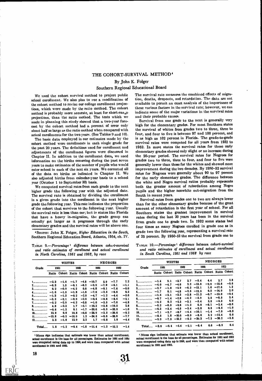
THE COHORT-SURVIVAL METHOD'
By John K. FolgerSouthern Regional Educational Board
We used the cohort survival method to project publicschool enrollment. We also plan to use a modification ofthe cohort method to revise our college enrollment projec-tions, which were made by the ratio method. The cohortmethod is probably more accurate, at least for short-rani4eprojections, than the ratio method. The tests which wemade in planning this study showed that a two-year fore-cast by the cohort method had a percent of error onlyabout half as large as the ratio method when compared withactual enrollments for the two years. (See Tables 9 and 10).
The basic data employed in our estimates made by thecohort method were enrollments in each single grade forthe past 20 years. The definitions used for enrollment andadjustments of the enrollment lignres were discussed inChapter II. In addition to the enrollment data, we usedinformation on the births occuring during the past sevenyears to make estimates of the number of pupils who wouldenter school in each of the next six years. We corrected allof the data on births as indicated in Chapter IL Wealso adjusted births from calendar-year basis to a schoolyear (October 1 to September 30) basis.
We computed survival rates from each grade to the nexthigher grade the following year with the adjusted date.The survival rate is obtained by dividing the enrollmentin a given grade into the enrollment in the next highergrade the following year. This rate indicates the proportionof the cohort that survives to the following year. Usuallythe survival rate is less than one; but in states like Floridathat have a heavy in-migration, the grade group canactually get larger as it progresses through the earlyelementary grades and the survival rates will be above one.
4Source: John K. Folger, Higher Education in the South,Southern Regional Education Board, Atlanta, 1954, ch. IV.
TAntx 9.--Percentage difference between colwrt-survivaland ratio estimates of enrollment and actual enrollmentin North Carolina, 1951 and 1962, by race
WHITES NEGROES
Grade 1951 1952 1951 1952
Ratio Cohort Ratio Cohott Ratio Cohort Ratio Cohort
l -2.3 -1.6 -1.7 -4.8 -10.7 5.9 -7.7 7.22 -6.3 1.3 -0.1 -0.2 -9.9 -7.0 -6.1 -1.13 0.2 -0.0 -4.2 0.8 -4.8 -0.1 -7.6 -5.04 -1.6 -1.5 -1.8 -1.6 -7.6 -2.5 -6.6 0.35 -1.3 -1.3 -0.2 -2.5 -4.7 -1.2 -4.4 -3.66 -3.3 -2.1 -0.0 -2.6 -6.4 -0.8 -8.4 -2.17 -5.2 -2.9 -4.2 -3.8 -1.0 -3.5 -7.6 -4.8s 4.8 -23 L7 -5.1 -16.3 -3.8 -19.5 2.89 -0.6 -1.2 0.1 -1.7 -35.6 -6.9 -33.9 -1.010 12.0 0.0 10.8 -0.8 -38.9 -3.5 -39.6 -9.2II -13.8 -0.2 -16.0 1.2 -34.5 -6.6 -38.6 -7.712 3.3 -1.0 12.9 3.2 1.7 -0.8 1.0 -4.4
TotaL 1.5 -1.2 -0.4 -1.8 -11.4 -1.3 -12.2 -1.4
I Minus sign indicates that estimate was lower than actual enrollment.actual enrollment is the base for all percentages. Estimates for 1951 and 1952were computed using data up to 1950, and were then compared with actualenrollment in 1951 and 1952.
18
3,1
The survival rate measures the conthined effects of migra-tion, deaths, dropouts, and retardation. The data are notavailable to permit an exact analysis of the importance ofthese various factors in the survival rate; however, we canindicate some of the major variations in the survival ratesand their probable causes.
Survival from one grade to the next is generally veryhigh for the elementary grades. For most Southern statesthe survival of whites from grades two to three, three tofour, and four to five is between 97 and 100 percent, andis as high as 102 percent in Florida. The grade-to-gradesurvival rates were computed for all years from 1932 to1952. In most states the survival rates for these earlyelementary grades showed only slight or no increase duringthe 20-year period. The survival rates for Negroes forgrades two to three, three to four, and four to five weregenerally lower than those for the whites and showed more
improvement during the two decadep. By 1950-52 survivalrates for Negroes were generally about 90 to 97 percentfor the early elementary grades. The difference betweenthe white and Negro survival ratios probably representsboth the greater amount of retardation among Negropupils and the higher nonwhite out-migration from theSouth in recent years.
Survival rates from grades onc to two are always lowerthan for the other elementary grades because of the greatamount of retardation in the first year of school. For allSouthern states the greatest improvement in survivalrates during the last 20 years has been in the survivalfrom grade one to grade two. In 1932 some states hadfour times as many Negroes enrolled in grade one as in
grade two the following year, representing a survival rateof 25 percent. By 1950-52 the survival from grade one to
Thum.: 10.-Percentagel difference between cohort-survivaland ratio estiniates of enrollment and actual enrollmentin South Carolina, 1951 and 1962 by race
WHITES NEGROES
Grade 1951 1952 1951 1952
Ratio Cohort Ratio Cohort Ratio Cohort Rtitio Cohort
1 -1.4 9.1 -3.7 3.7 -5.4 4.4 2.7 2.8
2 -4.0 -4.7 -4.0 2.2 -13.6 -2.9 -15.6 -5.63 -2.7 -1.0 -5.0 -0.2 -13.1 1.6 -17.6 1.3
4 -1.7 0.1 -4.8 -2.5 -12.5 0.5 -14.9 2.0
5 -1.5 -2.1 -3.3 -3.8 -11.2 -0.7 -13.0 -0.46 -0.7 -1.4 -2.8 -4.2 -5.9 2.5 -8.5 3.4
7 -4.2 0.2 -2.3 -3.1 -5.4 3.5 -5.3 6.0
8 . -5.2 -0.5 -9.6 -1.2 6.0 -8.1 -2.4 -8.69 -6.3 -3.4 -6.5 -3.4 -2.8 0.5 -0.5 -1.910 -7.1 -2.7 -8.7 -4.4 -10.1 -1.4 -7.9 -0.311 . -8.5 1.8 -10.6 -0.9 -8.6 3.2 -12.4 6.0
12 -9.9 -7.5 -13.2 -5.2 -20.3 -7.3 -20.2 -2.8 !
i
Total... -3.6 -0.4 -5.4 -2.1 -8.4 0.6 -8.0 0.4 >
!Minus sign indicates that estimate was lower than actual enrollment,actual enrollment is the base for all percentages. Estimates for 1951 and 1952
were computed using data up to 1950, and were then computed with actualenrollment in 1951 and 1952.
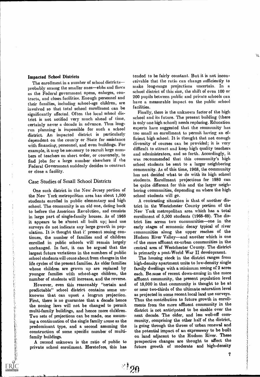
Impacted School DistrictsThe enrollment in a number of school districts
probably among the smaller onesebbs and flowsas the Federal government opens, enlarges, con-tracts, and closes facilities. Enough personnel andtheir families, including school-age children, areinvolved so that total school enrollment can besignificantly affected. Often the local school dis-trict is not notified very much ahead of time,certainly never a decade in advance. Thus long-run planning is impossible for such a schooldistrict. An impacted district is particularlydependent on the county or State for assistancewith financing, personnel, and even buildings. Forexample, it may be necessary to recruit large num-bers of teachers on short order, or conversely, tofind jobs for a large number elsewhere if theFederal Government suddenly decides to contractor close a facility.
Case Studies of Small School Districts
One such district in the New Jersey portion ofthe New York metropolitan area has about 1,500students enrolled in public elementary and highschool. The community is an old one, dating backto before the American Revolution, and consistsin large part of single-family houses. As of 1968it appears to be almost all built up; land usesurveys do not indicate any large growth in pop-ulation. It is thought that present zoning con-tinues, the number of families and of childrenenrolled in public schools will remain largelyunchanged. In fact, it can be argued that thelargest future variations in the numbers of publicschool students will come about from changes in thelife cycles of the present families. As older familieswhose children are grown up are replaced byyounger families with school-age children, thenumber of students will increase, and the reverse.
However, even this reasonably "certain andpredictable" school district contains some un-knowns that can upset a longrun projection.First, there is no guarantee that a decade hencethe zoning laws will not be changed to permitmulti-family buildings, and hence more children.Two sets of projections can be made, one assum-ing a continuation of the single family house as thepredominant type, and a second assuming theconstruction of some specific number of multi-family buildings.
A second unknown is the ratio of public toprivate school enrollment. Heretofore, this has
tended to be fairly constant. But it is not incon-ceivable that the ratio can change sufficiently tomake long-range projections uncertain. In a
school district of this size, the shift of even 100 or200 pupils between public and private schools canhave a measurable impact on the public schoolfacilities.
Finally, there is the unknown factor of the highschool and its future. The present building (thereis only one high school) needs replacing. Educationexperts have suggested that the community hastoo small an enrolhnent to permit having an ef-ficient high school. It is thought that not enoughdiversity of courses can be provided; it is verydifficult to attract. and keep high quality teachersand administrators, and so forth. Accordingly, itwas recommended that this community's highschool students be sent to a larger neighboringconununity. As of this time, 1968, the communityhas not decided what to do with its high schoolstudents. Enrollment projections for 1980 canbe quite different for this and the larger neigh-boring communities, depending on where the highschool students will go.
A contrasting situation is that of another dis-trict in the Westchester County portion of theNew York metropolitan area which has a totalenrollment of 5,500 students (1968-69). The dis-trict lies across two communitiesone in theearly stages of economic decay typical of rivercommunities along the upper reaches of theHudson River Valleyand another which is oneef the more affluent ex-urban conummities in thecentral area of Westchester County. The districtis primarily a post-World War II development.
The housing stock in the district ranges fromhigh-density apartment units to low-density singlefamily dwellings with a minimum zoning of 2 acreseach. Be Anse of recent down-zoning in the moreaffluent community, the present population levelof 18,000 in that community is thought to be ator near two-thirds of the ultimate saturation levelas projected in some recent local land use surveys.Thus the contribution to future growth in enroll-ments from the more affluent community in thedistrict is not antic;pated to be sizable over thenext decade. The older, and less well-off com-munity, comprising the other half of the district,is going through the throes of urban renewal andthe potential impact of an expressway to be builton land adjacent to the Hudson River. Theseprospective changes are thought to affect thefuture growth of moderate and high-density
7
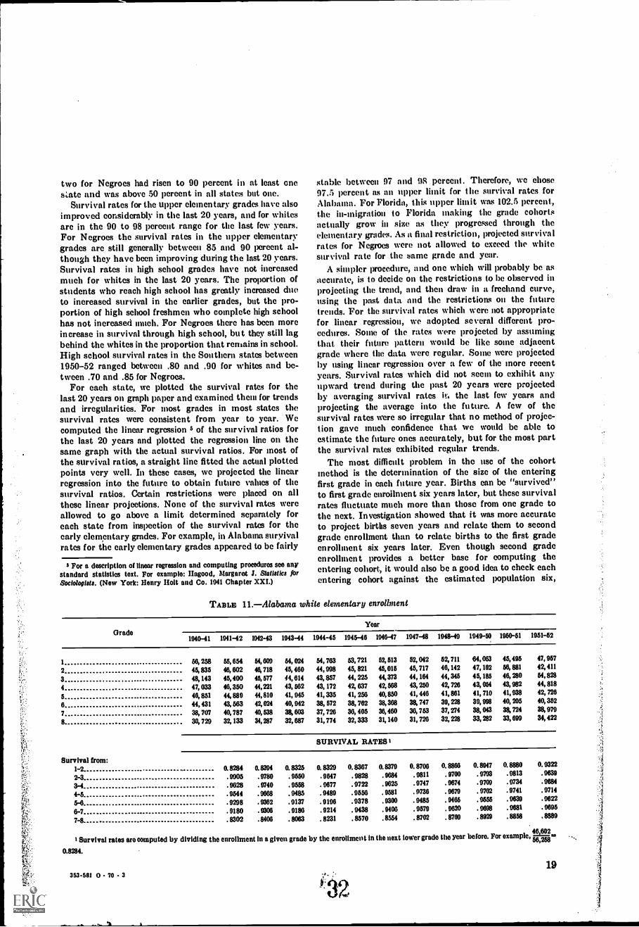
two for Negroes had risen to 90 percent in at least onesate and was above 50 percent in all states but one.
Survival rates for the upper elementary grades have alsoimproved considerably in the last 20 years, and for whitesare in the 90 to 98 percent range for the last few years.For Negroes the survival rates in the upper elementarygrades are still generally between 85 and 90 percent al-though they have been improving during the last 20 years.Survival rates in high school grades have not increasedmuch for whites in the last 20 years. The proportion ofstudents who reach high school has greatly increased dueto increased survival in the earlier grades, but the pro-portion of high school freshmen who complete high schoolhas not increased much. For Negroes there has been moreincrease in survival through high school, but they still lagbehind the whites in the proportion that remains in school.High school survival rates in the Southern states between1950-52 ranged between .80 and .90 for whites and be-tween .70 and .85 for Negroes.
For each state, we plotted the survival rates for thelast 20 years on graph paper and examined them for trendsand irregularities. For most grades in most states thesurvival rates were consistent from year to year. Wecomputed the linear regression 3 of the survival ratios forthe last 20 years and plotted the regression line on thesame graph with the actual survival ratios. For most ofthe survival ratios, a straight line fitted the actual plottedpoints very well. In these cases, we projected the linearregression into the future to obtain future values of thesurvival ratios. Certain restrictions were placed on allthese linear projections. None of the survival rates wereallowed to go above a limit determined separately foreach state from inspection of the survival rates for theearly elementary grades. For example, in Alabama survivalrates for the early elementary grades appeared to be fairly
3 For a description of linear regression and computing procedures see anystandard statistics text. For example: Hagood, Margaret J. Statistics forSociologists. (New York: Henry Holt and Co. 1941 Chapter XXI.)
stable between 97 and 98 . percent. Therefore, we chose97.5 percent as an upper limit for the survival rates forAlabama. For Florida, this upper limit was 102.5 percent,the in-migration to Florida making the grade cohortsactually grow in size as they progressed through theelementary grades. As a final restriction, projected survivalrates for Negroes were not allowed to exceed the whitesurvival rate for the same grade and year.
A simpler procedure, and one which will probably be asaccurate, is to decide on the restrictions to be observed inprojecting the trend, and then draw in a freehand curve,using the past data and the restrictions on the futuretrends. For the survival rates which were not appropriatefor linear regression, we adopted several different pro-cedures. Some of the rates were projected by assumingthat their future pattern would be like some adjacentgrade where the data were regular. Some were projectedby using linear regression over a few of the more recentyears. Survival rates which did not seem to exhibit anyupward trend during the past 20 years were projectedby averaging survival rates in the last few years andprojecting the average into the future. A few of thesurvival rates were so irregular that no method of projec-tion gave much confidence that. we would be able toe.stimate the future ones accurately, but for the most partthe survival rates exhibited regular trends.
The most difficult problem in the usc of the cohortmethod is the determination of the size of the enteringfirst grade in each future year. Births can be "survived"to first grade enrollment six years later, but these survivalrates fluctuate much more than those from one grade tothe next. Investigation showed that it was more accurateto project births seven years and relate them to secondgrade enrollment than to relate births to the first gradeenrollment six years later. Even though second gradeenrollment provides a better base for computing theentering cohort., it would also be a good idea to check eachentering cohort against the estimated population six,
TABLE 11.-Alabama white elementary enrollment
GradeYear
1940-41 1941-42 1042-43 1943-44 1944-45 1945-40 1040-47 1947-48 1948-49 1949-50 1950-51 1951-52
1 50, 258 55, 654 54, 009 54, 024 54, 763 53, 721 52, 513 52, 012 52, 711 64, 053 45, 495 47, 957
2 45, 835 46, 602 46, 718 45, 460 44, 998 45, 821 45, 015 45, 717 46, 142 47, 162 56, 881 42, 411
3 48, 143 45, 400 45, 677 44,614 43, 857 44, 225 44, 373 44, 164 44, 345 45, 185 46, 280 64,828
4 47, 033 46, 350 44, 221 43, 562 43, 172 42, 637 42, 568 43, 250 42, 726 43, 054 43, 982 44, 818
5 46, 851 44, 889 44,810 41, 945 41, 335 41, 256 40, 850 41, 446 41,861 41, 710 41, 938 42, 728
6 44, 431 43, 663 42, 024 40, 942 38, 672 38, 762 38, 368 38, 747 39, 228 39, 008 40, 205 40, 352
7 38, 707 40, 787 40, 638 38, 603 37, 726 36, 405 36,460 36, 763 37, 274 38, 043 38, 724 38, 979
8 30, 729 32, 133 34, 287 32, 687 31, 774 32,333 31, 140 31, 726 32, 228 33, 282 33, 699 34, 422
Survival from:1-22-33-44-55-66-77-8
SURVIVAL RATES I
0.8284 0.8394 0. 8325 0. 8329 0. 8367 0.8379 0. 8706 0. 8866 0.8047 0. 8880 0. 9322
.9905 .9780 .9550 .9647 .9828 .9684 .9811 .9700 .9793 .9813 .9639
9028 . 9740 . 9568 . 9677 . 9722 . 9625 . 9747 . 9674 . 9709 . 9734 . 9684
. 9544 . 9668 . 9485 . 9489 . 9556 . 9581 . 9736 . 9679 . 9762 . 9741 . 9714
9208 .9362 .9137 .9196 .9378 .9300 .9485 . 0465 .9555 .9639 . 9622
. 9180 . 9306 . 9186 . 9214 . 9438 . 9406 . 9579 . 9620 . 9698 . 9681 . 9695
. 8302 .8406 . 8063 . 8231 . 8570 .8554 . 8702 . 8709 . 8920 . 8868 . 8889
46,602
survival rates aro computed by dividing the enrollment In a given grade by the enrollment in the next lower grade the year before. For example, 50,258=
0.8284.
353-581 0 - 70 - 319
;')
apartment units which often yield fewer numbersof pupils per unit.
There is a great deal of uncertainty about theannual size of enrollments, particularly in theelementary grades, as well as the future existenceof the district itself, because:
First, New York State allows tuition transfersbetween adjacent, and in some instances, non-contiguous school districts depending uponvacancy levels. These tuition transfers have con-tributed to the annual variations of elementaryenrollments.
Second, several parochial school systems in thearea serviced by the school district have, due tofinancial uncertainties, recommended to parentsthat they enroll their children in public school forthe first grade and then transfer them into theparochial school system for the continuation oftheir education. This has the effect of overloadingexisting capcity levels in the kindergarten andfirst grades and drastically reducing capacitylevels in the second and later grades.
Third, the district has several wards in thepoorer of the two communities that are predomi-nantly nonwhite. As a result several of the neigh-borhood schools have reached unsafe white/non-white enrollment proportions as designated by theNew York State Department of Education. As a
8
result of this, redistribution through busing ofpupils to other schools in the district and adjacentdistricts is being contemplated.
Fourth, New York State Department of Ed-ucation facility planners have informed the localschool board that several of the existing facilitieshave become superannuated. The State EducationDepartment consultants have recommended tolocal school board officials a possible merger withan adjacent school district with newer, but rela-tively underutilized capacity levels.
All of these factors: the noncontiguity of localpolitical units and school districts; the economic,demographic and housing characteristics in thecommunities; the age and capacity of existing andcontemplated additions or changes in schoolplants; the very existence of the school district asa distinct entity; contribute to the difficulty ofgenerating reasonable, reliable, and comparableenrollment statistics series, and projections.
To some extent every school district is uniqueand has its own history. We have no reason tobelieve that the two districts described are partic-ularly unusual. They simply illustrate some of theproblems involved in trying to make enrollmentprojections for these semipermanent local publicschool districts.
21
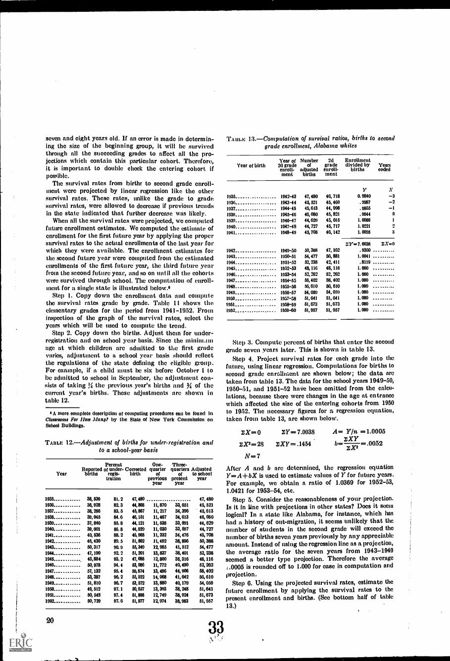
seven and eight years old. If an error is made in determin-ing the size of the beginning group, it will be survivedthrough all the succeeding grades to affect all the pro-jections which contain this particular cohort. Therefore,it is important to double check the entering cohort ifpossible.
The survival rates from births to second grade enroll-ment were projected by linear regression like the othersurvival rates. These rates, unlike the grade to gradesurvival rates, were allowed to decrease if previous trendsin the state indicated that further decrease was likely.
When all the survival rates were projected, we computedfuture enrollment estimates. We computed the estimate ofenrollment for the first future year by applying the propersurvival rates to the actual enrollments of the last year forwhich they were available. The enrolhnent estimates forthe second future year were computed from the estimatedenrollments of the first future year, the third future yearfrom the second future year, and so on until all the cohortswere survived through school. The computation of enroll-ment for a single state is illustrated below.6
Step 1. Copy down the enrollment data. and eomputethe survival rates grade by grade. Table 11 shows theelementary grades for the period from 1941-1932. Frominspection of the graph of the survival rates, select theyears which will be used to compute the trend.
Step 2. Copy down the births. Adjust them for under-registration and on school year basis. Since the minim.nnage at which children are admitted to the first gradevaries, adjustment to a school year basis should reflectthe regulations of the state defining the eligible group.For example, if a child must be six before October 1 tobe admitted to school in September, the adjnstment con-sists of taking 3.11 the previous year's births and of thecurrent year's births. These adjustments are shown intable 12.
A more complete description of computing procedures can be found inClassrooms For How Many? by the State of New York Commission onSchool Buildings.
TABLE 12.-Adjustment of births for under.registration andto a school-year basis
Percent One-Reported of under- Corrected quarter
Year births rests- birth oftration previous
year
Three-quarters Adjusted
of to schoolpresent year
year
1935 38, 539 81. 2 47,480 47, 4801936 36, 928 82. 3 44, 868 I I, 870 33, 651 45, 521
1937 38, 286 83. 6 45,867 II, 217 34, 396 45, 613
1938 39,045 84. 6 46,151 11,467 34, 613 46, 080
1939 37, 840 85. 8 44,121 11, 638 33,091 44, 6291940 39, 001 86. 8 44,929 11, 030 33,1197 44, 727
1941 40, 536 88. 2 45, 908 11, 232 34,476 45, 708
1942 46, 430 89. 5 51, 862 I I, 492 38, 896 50, 3881943 50, 317 90. 9 55,349 12, 965 41, 512 54, 477
1944 47, 190 92. 2 51, 201 13, 837 38, 401 52, 238
1945 43, 884 93. 2 47, 088 12, 800 35, 316 48, 1161946 50, 978 94. 4 53, 986 11, 772 40, 490 52, 262
1947 57, 132 95. 4 59,874 13, 496 44, 906 58, 402
1948 53, 387 96. 2 55, 522 14, 968 41, 642 56, 610
1949 51, 810 96. 7 53,572 13, NO 40, 179 54, 059
1950 49, 512 97. 1 50, 937 13, 393 38, 248 51, 641
1951 50, 548 97. 4 51, 898 12, 749 38, 924 51, 673
1952 50, 720 97. 6 51, 977 12, 974 38, 983 51, 957
20
TABLE 13.-Computation of survival ratios, births to secondgrade enrollment, Alabama whites
Year ofYear of birth 2d grade
enroll-nient
Numberof
adjustedbirths
2dgradeenroll-ment
Enrollmentdivided by
birthsYearscoded
Y X1935 1942-43 47, 480 46, 718 0. 9840 -31930 1943-44 45, 521 45, 460 . 9987 -21937 1944-45 45, 613 44, 998 . 9865 -I1938 1945-46 46, 080 45, 821 . 9944 0
1939 1946-47 44, 629 45, 015 I. 0086 1
1940 1947-48 44, 727 45, 717 I. 0221 2
1941 1948-49 45, 708 46, 142 I. 0095 3
3:Y=7. 0038 Z.V=01949 1949-50 50, 388 47, 162 . 9360
1943 1950-51 54, 477 56, 881 I. 0041
1944 1951-52 52, 238 42, 411 . 8119
1945 1952-53 48, 116 48, 116 I. 000
1946 1953-54 52, 269 52, 269 I. 000
1947 1954-55 58, 402 58, 402 I. 000
1948 1955-56 56, 610 56, 610 1.000
1949 1956-57 54, 059 54, 059 I. 000
1950 1957-58 51, 041 51, 041 I. 000
1951 1958-59 51, 673 51, 673 I. 000
1951 1959-60 51, 957 51, 957 I. 000
Step 3. Compute percent of births that enter the secondgrade seven years later. This is shown in table 13.
Step 4. Project survival rates for each grade into thefuture, using linear regression. Computations for births tosecond grade enrollment are shown below; the data aretaken from table 13. The data for the school years 1949-50,1950-51, and 1951-52 hrtre been omitted from the calm-lotions, because there were changes in the age at entrancewhich affected the size of the entering cohorts from 1950to 1952. The necessary figures for a regression equation,taken from table 13, are shown below.
2X= 0 2Y= 7.0038 A= Yin = 1.0005, 2
2
XY2X2= 28 2XY= .1454 0= -- .UUOZ
2XN=7
After A and b are determined, the regression equationY=A-FbX is used to estimate values of Y for future years.For example, we obtain a ratio of 1.0369 for 1952-53,1.0421 for 1953-54, etc.
Step 5. Consider the reasonableness of your projection.Is it in line with projections in other states? Does it seemlogical? In a state like Alabama, for instance, which hashad a history of out-migration, it seems unlikely that thenumber of students in the second grade will exceed thenumber of births seven years previously by any appreciableamount. Instead of using the regression line as a projection,the average ratio for the seven years from 1943-1949seemed a better type projection. Therefore the average.0005 is rounded off to 1.000 for ease in computation arid
projection.Step 6. Using the projected survival rates, estimate the
future enrollment by applying the survival rates to thepresent enrollment and births. (See bottom half of table13.)
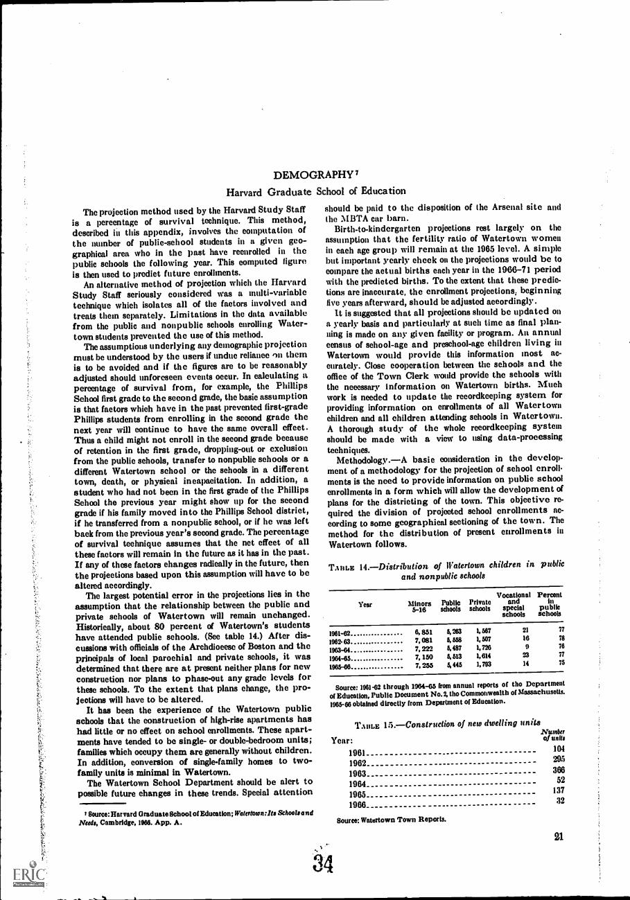
DEMOGRAPHY 7
Harvard Graduate School of Education
The projection method used by the Harvard Study Staffis a percentage of survival technique. This method,described in this appendix, involves the computation ofthe munber of public-school students in a given geo-graphical area who in the past have reenrolled in thepublic schools the following year. This computed figureis then used to predict future enrollments.
An alternative method of projection which the HarvardStudy Staff seriously considered was a multi-variabletechnique which isolates all of the factors involved andtreats them separately. Limitations in the data availablefrom the public and nonpublic schools enrolling Water-town students prevented the use of this method.
The assumptions underlying any demographic projectionmust be understood by the users if undue reliance m themis to be avoided and if the figures are to be reasonablyadjusted should unforeseen events occur. In calculating apercentage of survival from, for example, the PhillipsSchool first grade to the second grade, the basic assumptionis that factors which have in the past prevented first-gradePhillips students from enrolling in the second grade thenext year will continue to have the same overall effect.Thus a child might not enroll in the second grade becauseof retention in the first grade, dropping-out or exclusionfrom the public schools, transfer to nonpublic schools or adifferent Watertown school or the schools in a differenttown, death, or physicai incapacitation. In addition, astudent who had not been in the first grade of the PhillipsSchool the previous year might show up for the secondgrade if his family moved into the Phillips School district,if he transferred from a nonpublic school, or if he was leftback from the previous year's second grade. The percentageof survival technique assumes that the net effect of allthese factors will remain in the future as it has in the past.If any of these factors changes radically in the future, thenthe projections based upon this assumption will have to bealtered accordingly.
The largest potential error in the projections lies in theassumption that the relationship between the public andprivate schools of Watertown will remain unchanged.Historically, about 80 percent of Watertown's studentshave attended public schools. (See table 14.) After dis-cussions with officials of the Archdiocese of Boston and theprincipals of local parochial and private schools, it wasdetermined that there are at present neither plans for newconstruction nor plans to phase-out any grade levels forthese schools. To the extent that plans change, the pro-jections will have to be altered.
It has been the experience of the Watertown publicschools that the construction of high-rise apartments hashad little or no effect on school enrollments. These apart-ments have tended to be single- or double-bedroom units;families which occupy them are generally without children.In addition, conversion of single-family homes to two-family units is minimal in Watertown.
The Watertown School Department should be alert topossible future changes in these trends. Special attention
7 Source:Harvard Graduate School of Education; Watertown:Its Schools andNeeds, Cambridge, 1966. App. A.
should be paid to the disposition of the Arsenal site andt he MBTA car barn.
Birth-to-kindergarten projections rest largely on theassumption that the fertility ratio of Watertown womenin each age group will remain at the 1965 level. A simplebut important yearly cheek on the projections would be tocompare the actual births each year in the 1966-71 periodwith the predicted births. To the extent that these predic-tions are inaccurate, the enrollment projections; beginningfive years afterward, should be adjusted accordingly.
It is suggested that all projections should be updated ona yearly basis and particularly at such time as final plan-ning is made on any given facility or program. An annualcensus of school-age and preschool-age children living inWatertown would provide this information most ac-curately. Close cooperation between the schools and theoffice of the Town Clerk would provide the schools withthe necessary information on Watertown births. Muchwork is needed to update the recordkeeping system forproviding information on enrollments of all Watertownchildren and all children attending schools in Watertown.A thorough study of the whole recordkeeping systemshould be made with a view to using data-processingtechniques.
Methodology.A basic consideration in the develop-ment of a methodology for the projection of school enroll.ments is the need to provide information on public schoolenrollments in a form which will allow the development of
plans for the districting of the town. This objective re-quired the division of projected school enrollments ac-cording to some geographical sectioning of the town. Themethod for the distribution of present enrollments inWatertown follows.
TABI.E 14.Distribution of Watertown children in publicand nonpublic schools
YearVocational Percent
Minors Public Private and in5-16 schools schools special public
schools schools
1961-62 6, 851 5,263 UV 21 77
1962- 63 7, 081 5, 558 1, 507 16 78
1963-64 7, 222 5,487 1, 726 9 76
1964-65 7, 150 5,513 1,614 23 77
1965-66 7,255 5, 445 1, 703 14 75
Source: 1961-62 through 1964-65 from annual reports of the Departmentof Education, Public Document No. 2, the Commonwealth of Massachusetts.
1965-66 obtained directly from Department of Education.
T.timE 15.Construction of new dwelling units
Year:1961-19621963196419651966
34
Source: Watertown Town Reports.
Numberof units
104
295
36652
13732
21
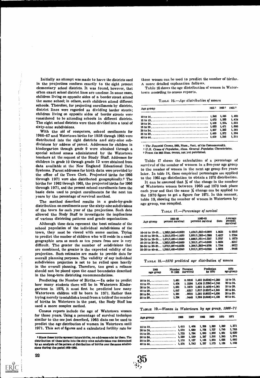
Initially an attempt was made to have the districts usedin the projections conform exactly to the eight presentelementary school districts. It was found, however, thatoften exact school district lines afe unclear. In some eases,children living on opposite sides of a border street attendthe same school; in others, such children attend differentschools. Therefore, for projecting enrollments by districts,district lines were regarded as dividing border streets;children living on opposite sides of border streets wereconsidered to be attending schools in different districts.The eight school districts were then divided into a total ofsixty-nine subdivisions.
With the aid of computers, school enrollments for1966-67 and Watertown births for 1958 through 1965 weredistributed into the eight districts and sixty-nine sub-divisions by address of parent. Addresses for children inkindergarten through grade 9 were obtained through aspecial school census administered by the Watertownteachers at the request of the Study Staff. Addresses forchildren in grade 10 through grade 12 were obtained fromdata available at the New England Educational DataSystems. Parent addresses for birth data were provided bythe office of the Town Clerk. Projected births for 1966through 1971 were also distributed geographically.8 Thebirths for 1962 through 1965, the projected births for 1966through 1971, and the present school enrollments form thebasic data used to project enrollments for the next tenyears by the percentage of survival method.
The method described results in a grade-by-gradedistribution on enrollments over the sixty-nine subdivisionsof the town for each year of the projections. Such dataallowed the Study Staff to investigate the implicationsof various districting patterns and grade organizations.
Although these data represent the best estimate of theschool population of the individual subdivisions of thetown, they must be viewed with some caution. Tryingto predict the number of children who will reside in a smallgeographic area as much as ten years from now is verydifficult. The greater the number of subdivisions thatare combined, the greater is the expected validity of theprojection. Such estimates are made to provide data foroverall planning purposes. The validity of any individualsubdivision projection is not to be relied upon heavilyin the overall planning. Therefore, too great a relianceshould not be placed upon the exact boundaries describedin the long-term districting recommendations.
Predicting the Number of Births.-In order to predicthow many students there will be in Watertown Kinder-gartens in 1976, it must first be predicted how manyWatertown children will be born in 1971. Rather thantrying merely to establish a trend from a table of the numberof births in Watertown in the past, the Study Staff hasused a more complex method.
Census reports include the age of Watertown womenfor those years. Using a percentage of survival techniquesimilar to the one just described, 1965 data can be used topredict the age distribution of women in Watertown until1971. This set of figures and a calculated fertility rate for
Since these births represent future births, no addresses exist for theni. Thedistribution of these births into the sixty-nine subdivisions was determinedby an analysis of the pattern of distribution of births over the same subdivi-sions duting the period 1958-1965.
these women can be used to predict the number of births.A more detailed explanation follows.
Table 16 shows the age distribution of women in Water-town according to census reports.
TABLE 16.-1ge distribution of women
Ago group 1955 1 1960 2 1905 3
10 to 14. 1,346 1,565 1, 481
15 to 19 1,073 1,283 1,42420 to 24 1,409 1, 25L 1,651
25 to 29. 1,633 1,471 1,66630 to 34 1,007 1,383 1,201
35 to 39. 1,409 1,372 1,204
40 to 44 1,429 1,316 1,311
I The Decennial Census, 1055, Mass., Sect. of the Commonwealth.U.S. Come of Population, Mau. General Population Characteristics.
3 From the 1905 Mass. census, not yet published.
Table 17 shows the calculation of a percentage ofsurvival of the number of women in a five-year age groupto the number of women in the next age group five yearslater. In table 18, these empirical percentages are appliedto the 1966 age distribution to obtain a 1970 distribution.
It can be assumed that g of the change in the numberof Watertown women between 1965 and 1970 took placeeach year and that the same g change can be applied tothe 1970 figure to get a figure for 1971. In this manner,table 19, showing the number of women in Watertown byage group, was compiled.
TABLE 17.-Percentage of survival
Ago group1955-60
lwrcent survival1060-05
percent survival BuntAveragepercentsurvival
10-14 to 15-19... 1,283/1,346..0.9532 1,424/1,565..0.9099 1.8631 0.931615-19 to 20-24... 1,251/1,073..1.1650 1,651/1,283..1.2868 2.4527 1.2264
20-24 to 25-29... 1,471/1,409..1.0440 1,666/1,251..1.3317 2.3757 1. 1879
25-29 to 30-34... 1,383/1,633.4.8469 1,201/1,471..0.8165 1.6634 .8317
30-34 to 35-39... 1,372/1,607..0.8538 1,204/1,383..0.8700 1. 7244 . 8622
35-39 to 4044... 1,316/1,409.0.9340 1,311/1,372..0.9555 1.8895 .9448
TABLE 18.-1070 predicted age distribution of women
1965age group
Number Percentin 1965 survival
Predictionfor 1970
1970ago group
10 to 14 1,481 0.9316 1,481 (0.9316)=4,380 15 to 19.
15 to 19 1,424 1.2264 1,424 (1.2264)=4,746 9) to 24.
20 to 24 1,651 1.1879 1,651 (1.1879)..1.96l 25 to 29.
25 to 20 1,617 .8317 1,617 (0.8317)=.1,345 30 to 34.
30 to 34 1,201 .8622 1,201 (0.8622) ..1,036 35 to 39.
35 to 39 1,204 .9448 1,204 (0.9448)=.1,138 40 to 44.
TABLE 19.-Women in Watertown by age group, 1066-71
Age group 1966 1967 1968 1909 1970 1971
15 to 19 1,415 1, 406 1,398 1,389 1,380 1,371
20 to 24 1, 670 1, 689 1, 7013 1, 727 1, 746 1, 765
25 to 29 1,725 1, 784 1,843 1,902 1,961 2,020
30 to 34. 1,230 1,259 1,217 1,316 1,345 1,374
35 to 39 1,170 1,137 1,103 1,070 1,036 1,002
40 to 44 1,276 1,242 1,207 1,173 1,138 1,103
2235
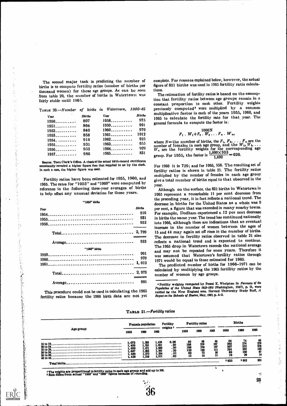
The second major task in predicting the number ofbirths is to compu te fertility ratios (number of births perthousand women) for these age groups. As can be seenfrom table 20, the number of births in Watertown wasfairly stable until 1965.
TABLE 20.NumberYear
of births in Watertown, 1950-65
Births Year Births
1950 807 1958 975
1951 864 1959 991
1952 840 1960 970
1953 858 1961 1012
1954 916 1962 925
1955 931 1963 955
1956 952 1964 929
1957 986 1965 831
Source: Town Clerk's Office. A chock of tho actual birth-record certificatesoccasionally revealed a higher figure than that supplied to us by tho clerk.In such a case, tho higher figure was used.
Fertility ratios have been estimated for 1955, 1960, and1965. The rates for "1955" and "1960" were computed byreference to the following three-year averages of birthsto help offset any unusual deviation for those years.
"1966" births
Year
195419551956
Births
916931952
Total_ 2, 799
Average 933
"1960" births
1959 991
1960 970
1961 1, 012
Total 2, 973
Average 991
This procedure could not be used in calculating the 1965fertility ratios because the 1966 birth data are not yet
complete. For reasons explained below, however, the actualfigure of 831 births was used in 1965 fertility ratio calcula-
tions.The estimation of fertility ratios is based on the assump-
tion that fertility ratios between age groups remain in aconstant proportion to each other. Fertility weights
previously computed were multiplied by a commonmultiplicative factor in each of the years 1955, 1960, and1965 to calculate the fertility rate for that. year. Thegeneral formula to compute the factor is;
1000NF1 . W1-142 . W2. . . Wn,
where N= the number of births, the F1, F2, . . . F are thenumber of females in each age group, and the WI, 11'2, . . .
11f are the fertility weights for the corresponding age1,000X 933 626.group. For 1955, the factor is 1,490
For 1960 it is 729; and for 1965, 556. The resulting set offertility ratios is shown in table 21. The fertility ratiosInultiplied by the number of females in each age groupgive a total number of births equal to that observed in the
year.Although on the surface, the 831 births in Watertown in
1965 represent a remarkable 11 per cent decrease fromthe preceding year, it in fact reflects a national trend. Thedecrease in births for the United States as a whole was 9
per cent, a figure that was exceeded in many nearby towns.For example, Dedhani experienced a 12 per cent decreasein births the same year. The trend has continued nationallyinto 1966, although there arc indications that an eventualincrease in the number of women between the ages of
15 and 44 may again set off rises in the number of births.The decrease in fertility ratios observed in table 21 alsoreflects a national trend and is expected to continue.The 1965 drop in Watertown exceeds the national averageand may not be repeated for some years. Therefore itwas assumed that Watertown's fertility ratios through1971 would be equal to those estimated for 1965.
The predicted number of births for 1966-1971 can be
calculated by multiplying the 1965 fertility ratios by thenumber of women by age groups.
*Fertility weights computed by Poscal K. Wholpton in Forecasts of the
Population of the United States 1848-1978 (Washington, 1947), p. 21, were
verified for the New England area. Harvard University Study Staff, A
Report on the Schools of Boston, May, 1962, p. A-3.
TABLE 21.Fertility ratios
Ago groupFemale Population Fertility
weightsFertility ratios Births
1955 1960 1965 1055 1960 1965 1955 1960 INS
e 15 to 19 . 1,073 1,283 1,424 0.08 ao as 44 64 74 63
20 to 24 1,409 1,251 1,651 .30 188 219 167 265 274 276
et, 25 to 29 1,633 1,471 1,666 .30 188 219 167 307 322 278
30 to 34 1,607 1,383 1,201 . 20 123 146 III 201 202 133
35 to 39 1,409 1,372 1,204 10 63 73 sa 89 100 67
40 to 44 1,429 1,316 1,311 .02 13 15 II 19 20 14
Total births3 935 $ 992 831
I The weights are proportional to fertility ratios in each age group and add up to 100.Sum differs from actual "1955" and "1960" figures because of rounding.
24
36
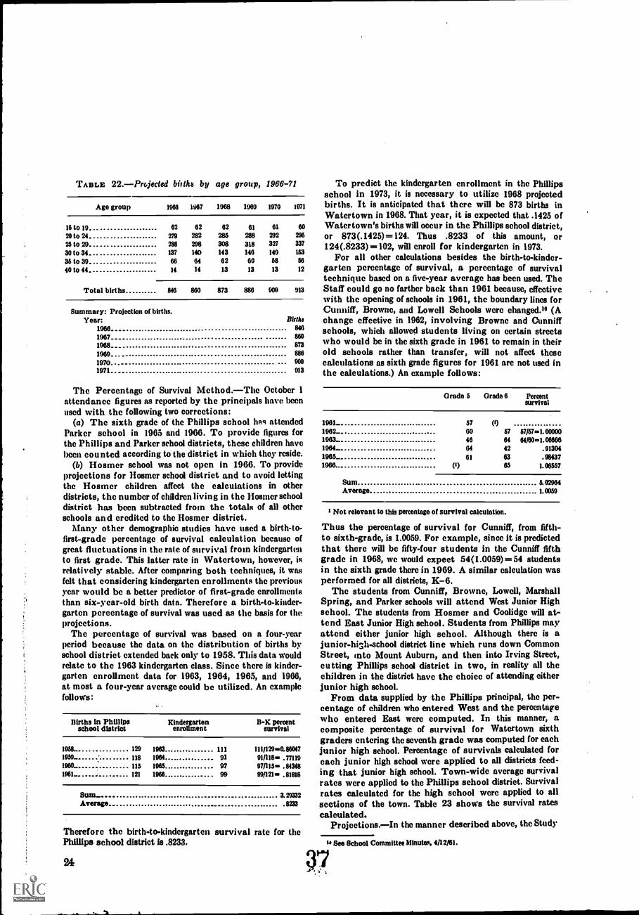
TABLE 22.Projecte4 billhe by age group, 1966-71
Age group 1066 1067 1068 1969 1970 1971
16 to 19 62 62 62 61 61 60
20 to 24 279 282 285 288 292 295
25 to 29 288 298 308 318 327 337
301034 137 140 143 146 149 163
36 to 39 66 64 62 60 68 56
40 to 44 14 14 13 13 13 12
Total births 846 860 873 886 900 913
Summary: Projection of births.Year: Births
1966 846
1967 860
1068 873
1969 886
1970. . 000
1971. 013
The Percentage of Survival Method.The October 1attendance figures as reported by the principals have beenused with the following two corrections:
(a) The sixth grade of the Phillips school hns attendedParker school in 1965 and 1966. To provide figures forthe Phillips and Parker school districts, these children havebeen counted according to the district in which they reside.
(b) Hosmer school was not open in 1966. To provideprojections for Hosmer school district and to avoid lettingthe Hosmer children affect the calculations in otherdistricts, the number of children living in the Homer schooldistrict has been subtracted from the totals of all otherschools and credited to the Hosmer district.
Many other demographic studies have used a birth-to-first-grade percentage of survival calculation because ofgreat fluctuations in the rate of survival from kindergartento first grade. This latter rate in Watertown, however, isrelatively stable. After comparing both techniques, it wasfelt that considering kindergarten enrollments the previousyear would be a better predictor of first-grade enrollmentsthan six-year-old birth data. Therefore a birth-to-kinder-garten percentage of survival was used as the basis for theprojections.
The percentage of survival was based on a four-yearperiod because the data on the distribution of births byschool district extended back only to 1958. This data wouldrelate to the 1963 kindergarten class. Since there is kinder-garten enrollment data for 1963, 1964, 1965, and 1966,at most a four-year average could be utilized. An examplefollows:
Births in Phillipsschool district
Kindergartenenrollment
B-IC percentsurvival
1058_ 129 1963 111 111/1200.860171959 118 1964 91 011118 .771191960 115 1065 97 071115 .843481961 121 1966 99 119/121 .81818
Sum_ 3.29332Average_ 8233
Therefore the birth-to-kindergarten survival rate for thePhillips school district is .8233.
24
To predict the kindergarten enrollment in the Phillipsschool in 1973, it is necessary to utilize 1968 projectedbirths. It is anticipated that there will be 873 births inWatertown in 1968. That year, it is expected that .1425 ofWatertown's births will occur in the Phillips school district,or 873(.1425)=124. Thus .8233 of this amount, or124(.8233)=102, will enroll for kindergarten in 1973.
For all other calculations besides the birth-to-kinder-garten percentage of survival, a percentage of survivaltechnique based on a five-year average has been used. TheStaff could go no farther back than 1961 because, effectivewith the opening of schools in 1961, the boundary lines forCunniff, Browne, and Lowell Schools were changed.0 (Achange effective in 1962, involving Browne and Cunniffschools, which allowed students living on certain streetswho would be in the sixth grade in 1961 to remain in theirold schools rather than transfer, will not affect thesecalculations as sixth grade figures for 1961 are not used inthe calculations.) An example follows:
Grade 5 Grade 6 Percentsurvival
1961 57 (91962 60 67 67/67-1. 000001963 46 64 04/60...1.066661964 64 42 .913041965 61 63 .984371966 (9 85 1.06557
Sum 5.02964Average 1.0059
1 Not relevant to this percentage of survival calculation.
Thus the percentage of survival for Cunniff, from fifth-to sixth-grade, is 1.0059. For example, since it is predictedthat there will be fifty-four students in the Cunniff fifthgrade in 1968, we would expect 54(1.0059)=54 studentsin the sixth grade there in 1969. A similar calculation wasperformed for all districts, K-6.
The students from Cunniff, Browne, Lowell, MarshallSpring, and Parker schools will attend West Junior Highschool. The students from Hosmer and Coolidge will at-tend East Junior High school. Students from Phillips mayattend either junior high school. Although there is ajunior-high-school district line which runs down CommonStreet, into Mount Auburn, and then into Irving Street,cutting Phillips school district in two, in reality all thechildren in the district have the choice of attending eitherjunior high school.
From data supplied by the Phillips principal, the per-centage of children who entered West and the percentagewho entered East were computed. In this manner, acomposite percentage of survival for Watertown sixthgraders entering the seventh grade was computed for eachjunior high school. Percentage of survivals calculated foreach junior high school were applied to all districts feed-ing that junior high school. Town-wide average survivalrates were applied to the Phillips school district. Survivalrates calculated for the high school were applied to allsections of the town. Table 23 shows the survival ratescalculated.
Projections.In the manner described above, the Study
u see School Committee Minutes, 4112/61.
J
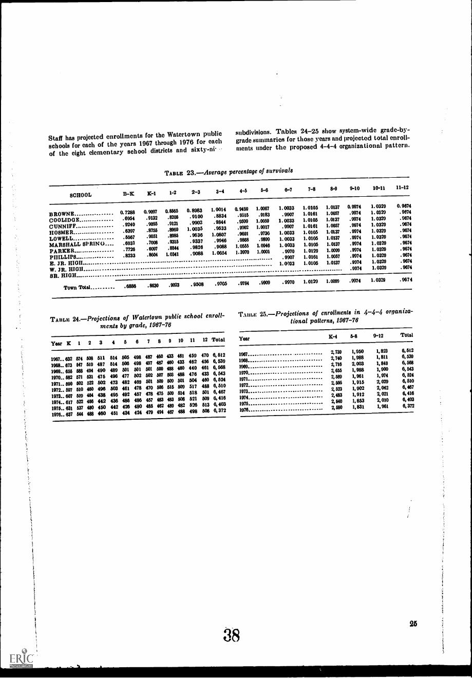
Staff has projected enrollments for the Watertown publicschools for each of the years 1967 through 1976 for each
of the eight elementary school districts and sixty-ni.
subdivisions. Tables 24-25 show system-wide grade-by-grade summaries for those years and projected total enroll-ments under the proposed 4-4-4 organizational pattern.
TABLE 23.-Average percentage of survivals
SCHOOL B-K K-1 1-2 2-3 3-4 4-5 5-6 6-7 7-8 8-0 9-10 10-11 11-12
BROWNE 0. 7288 0.9097 0.8585 0. 8983 I. 0014 0.9459 1.0007 1. 0033 1. 0105 1.0137 0.9974 1. 0329 0. 9874
COOLIDGE .8954 .0132 .8205 .9100 .8834 .9515 .9183 .9907 1.0161 1.0057 .9974 1.0329 .9674
CUNNIFF .9240 .9095 .9121 .9902 .9844 .0599 1.0059 1.0033 1.0105 1.0137 .9974 1.0329 .9674
HOENE R .8397 .8755 .8989 1.0035 .9533 .9902 1.0017 .9907 1.0161 1.0057 .9974 1.0329 .9674
LOWELL 5587 .9051 .8085 .9836 1.0807 .9891 .9736 1.0033 1.0105 1.0137 .9974 1.0329 .9874
MARSHALL SPRING .6931 .7008 .9315 .9337 .9946 .9888 .9899 1.0033 1.0105 1.0137 .9974 1.0329 .9674
PARKER . 7726 .8097 .8844 .9826 .9088 1.0556 1.0946 1.0033 1.0105 1.0137 .9974 1.0329 .9674
PHILLIPS 8233 .8804 1.0341 .9088 1.0654 1.3970 1.0001 .9970 1.0129 1.0099 .9974 1.0320 .9674
E. JR. RIM!.9907 1.0161 1.0057 .9974 1.0329 .9874
W. JR. 1110111.0433 1.0105 1.0137 .9974 1.0320 .9874
SR. HIGH ..9974 1.0329 .9674
Town Total .6886 .8830 .9023 .9508 .9705 .9784 .0909 .9970 1.0129 1.0099 .9974 1.0329 . 9674
TAmai 24.-Projections of Watertown public school enroll-ments by grade, 1967-76
TABLE 25,-Projections of enrollments in 4-4-4 organiza-tional patterns, 1967-76
Year K 1 2 3 4 6 6 7 8 9 10 11 12 Total Year IC-4 6-8 9-12 Total
1987.. 832 574 508 511 514 505 498 487 480 433 461 459 470 6, 512 1987 *,739 1,950 1,823 6,612
1988.. 873 647 619 487 514 506 498 497 487 480 433 462 458 6,539 1988*, 740 1,988 1,811 6, 530
1969.. 665 688 494 490 489 501 501 501 600 488 480 440 461 6, 668 19802, 716 2, 003 1,849 6,588
1970.. 582 671 531 475 496 477 502 602 507 503 488 478 433 8, 543 1970 2,855 1,988 1,900 6, 543
1971.. 590 602 522 502 473 482 469 501 609 509 601 504 480 6, 524 19712,589 1, 961 1,974 6, 524
1972.. 597 610 480 498 603 481 478 470 508 616 509 517 488 6, 610 19722,688 1,915 2,029 6,610
1973.. 807 619 484 438 495 492 457 478 475 509 614 618 501 6,467 19732,523 1,902 2,042 8, 487
1974.. 817 622 488 442 438 488 488 467 483 483 608 521 609 6,418 19742,483 1,912 2,021 6,418
1975.. 631 637 480 450 442 428 480 485 482 489 482 626 513 6, 403 19752, 540 1,853 2,010 6,403
1978.. 837 514 488 480 461 434 424 479 494 487 488 498 508 6,372 19782,580 1,831 1,961 6, 372
26
CHAPTER 4
SHORT-RANGE SCHOOL ENROLLMENT PROJECTIONTECHNIQUES CONTINUED: DWELLING-UNIT
ENROLLMENT-YIELD MULTIPLIERS
Another approach for making shortrun pro-jections is through the use of information on theinventory of housing in the community, and theaverage number of pupils yielded by each type ofhousing, for example, one-family dwellings vs.apartment houses. This approach has particularmerit for those local school areas undergoingsubstantial growth in the development of theland-space of the community or for those com-munities whose annual fluctuations in enrollmentare geared to significant fluctuations in theemployment size of the local work force; forexample, "federally-impacted" communities, areaswith a substantial segment of the employmentbase consisting of civilian or military personnelassigned to federal facilities. For these com-munities, the dwelling-unit, enrollment-yield meth-od of forecasting school enrollment often canprovide useful information for planning the timingfor school construction, as well as for schoolpersonnel recruitment and development.
Ideally, a community should use both ap-proachesthe cohort-survival and the dwelling-unit enrollment. Each method is fairly independentof the other, thereby providing a check. Bothtechniques should provide reasonably similarprojections for the target date in order to insureconfidence in the estimates. This is especially soif the target date is no more than 5 years in thefuture. If, for example, both indicate that enroll-ment will increase about 15 percent in the following5 years, then school officials can be reasonablyconfident of the projection. On the other hand, ifone technique suggests an increase of about 5percent, and the other one of 15 percent, then theschool officials are in a dilemma. Neither set oftechniques can be demonstrated to he inherently
more accurate than the other. Accordingly, onlya careful subjective appraisal using'all informationavailable to the community can suggest whatmay be the best estimate.
In this chapter we shall cover some basictopics along with two examples of the applicationof the approach. They are: first, general informa-tional and organizational requirements of theapproach; second, the derivation of pupil-yieldmultiples for estimating school facility capacitiesin Montgomery County, Md., and for local areasin California.
Housing Inventories and Land-Use SurveysThe technique, "dwelling-unit enrollment-yield
multipliers," taking as it does existing and antici-pated construction into account, is really a land-use survey applied to school enrollment projections.Many communities conduct such surveys forpurposes of planning roads, police and fire service,and other public services. Private organizationsuse information on how the land is being utilizedat present, and how it might be utilized in thefuture, for planning the opening of retail stores tothe installation of telephone cables, and so forth.By the simple device of using the type of dwellingunit to estimate the probable number of childrenenrolled in public schools, the land-use surveybecomes a technique for projecting schoolenrollment.
Note also that this technique is most useful forthe shortrun period, perhaps 2 to 5 years ahead.It is useful to the extent that construction workhas begun, building permits issued, or housingdevelopment seriously contemplated. For longer-range periods, the land-use survey becomes largelyjudgmental. When-5, 10, 20 years hencewill a
given parcel of land be developed? And will it befor single-family detached structures or someother construction? Zoning laws stipulate the typeof permissible structure, but what is to preventthe present zoning laws from being changed 10years from now?
An interesting methodology is being tested inBucks County, Pa., for making longrun projec-tions based on present and future housing supply.The report"Estimate of Future PopulationGrowth by School District, Bucks County, Penn-sylvania"describing the methodology is givenin appendix D. The authors wrote:
This estimate of population growth by school districtdepends on a methodology which is still under development
(italics ours) but is consistent with results produced byspecial censuses taken in Bucks County since 1960.
How useful these procedures may be for othercounties or communities is difficult to say since,apparently, Bucks County and the rest of thePhiladelphia Standard Metropolitan Area is theonly part of the country where this has been tried.Perhaps one of the reasons why other counties hadnot tested it since 1960 is that special censusespast 1960are required, as well as numbers ofbuilding permits. Furthermore, intimate and de-tailed knowledge of the local area is required.Perhaps after the 1970 Decennial Census resultsbecome available, other communities may be ableto test the method.
It should also be noted that it is not certain thatthis method can be applied to asmall area withouttaking into consideration the county or region ofwhich it is a part. The authors wrote:
It is an open question whether there is any such thingas a purely local trend in the development of a smallarea's population. The population growth of a small areaappears to depend not only on the growth of its ownhousing supply but also on the provision of housing inmany, many other small areas.
General Information RequirementsTo begin, there must be considerable coopera-
tion and communication with the local construc-tion and real estate industry. Foreknowledge offuture real estate development expansion, in
conjunction with the pupil-yield characteristics ofthe intended housing, will aid school planners inthe location and acquisition of site facilities anddetermination of local school transportation needs.A good example of this is the enabling legislationof Dade County, Fla. which requires submissionof real estate development plans to the countyschool planners. Thus, they can evaluate theeffects
of the intended development upon future schoolenrollment, facilities, and other needs.
Second, information also should be obtained onthe destruction of housing. If it is known that alarge area of houses is to be cleared in order toprovide new highways or bridge approaches, thatinformation may be as important, or more so, than
the numbers of new dwelling units scheduled forconstruction. Furthermore, if existing buildingsare to be torn down and replaced with a different
type of dwelling unit, that too should be knownin advance. With such information, estimates ofthe probable loss in public school enrollment canbe set alongside information on the possible gain.
Third, the use,. of the dwelling-unit enrollment-
yield multiplier approach must be intimatelyaware of the housing cycle of the local community.This is perhaps best illustrated by the case ofMontgomery County, Md. The 1960 medianfamily income of $9,340 and educational attain-ment levels of 13.3 years for men and 12.6 yearsfor women (population aged 25 and over) placesthe county among the highest in the Nation inthese two characteristics. Until the early 1960'sthe county served largely as a bedroom for FederalGovernment employees. However, with the rapidgrowth of a federally-supported science-basedindustrial complex, the community grew morerapidly and took on a different character. Let usexamine some aspects.
In the lower third of the county, immediately
adjacent to the District of Columbia, older,
previously expensive housing began to depreciatein value, falling to a price range which relatively
young large families could afford. The result wasthat schools in this area experienced a relativelyrapid increase in enrollments, particularly in theelementary grades.
In another portion of the lower third of thecounty, a somewhat different phenomenon wasgoing on. Surveys of an intensive built-up areacomprised of high-rise apartment units and popu-lated largely by young families of moderate incomelevels consistently overestimated the number oftransfers of pupils from kindergarten to first grade.
In one survey an expected number of 400 first
grade entrants in a particular school from thepreceding spring term of kindergarten dwindled toless than 40 by the start of the fall ter»). Thoapparent cause of this massive out-migration wasthat many families with children, ages 4 to 6,purchased single-family dwellings and moved toother areas of the county served by other schools.
27
Since the several school buildings were part of thesame school distiict, however, the total enroll-ment for the entire district was not affected.
The county development board approved thecreation of a new form of dwelling unit known asan apartment hotel. School planners in Mont-gomery County, after consultation with severaldevelopers interested in the construction of suchunits, anticipated a substantial drop in the pupil-yields from such units. The major reason is thatthe units are geared to the demands of puddle-to-older-age persons and to couples who are wellpast the child-rearing stage of the family life cycle.
Another example of the effects of the family lifecycle is given in the Bucks County report (ap-pendix D). Despite the increase in populationbetween 1960 and 1965, school enrollment in-creased only by the amount expected on the basisof the number of preschool age children, under age5, living in the county in 1960. The authorsexplain this apparent contradiction by statingthat, "The major trend 1960-1965 in school en-rollments has had to do with the aging of theresident population."
It would thus appear that intimate knowledgeof the local housing cycle in conjunction with somegeneral knowledge of family life-cycle behaviorparticularly on the question of timing of housingpurchaseswould aid school planners in the de-sign and conduct of dwelling-unit surveys, as wellas the exploitation of local building-developmentinformation.
Use of Dwelling-Unit Pupil-Yield Multipliers
Montgomery County, Md.The Montgomery County Educaticnal Services
Administration through its Division of Planninghas had considerable experience using the dwelling-unit pupil-yield multiplier approach for projectingenrollments for its 160 or more schools.
To accomplish this the Division of Planningdivided the county into 12 educational planningregions. Each planning region consists of severalelementary and secondary schools, as well as anumber of kindergarten units. In some casesplanning regions were established in portions ofthe county which have only recently (latter1960's) been developed, but which are expectedto grow during the next 5 to 7 years. As a resultseveral of these planning regions have onlykindergarten and elementary facilities. However,sites for the acquisition of secondary facilities are
28 41
already, or are currently (1968) in various stagesof being programed.
The planning division has placed the planningregions onto several dozen grid squares coin parablewith the 1:200 scale maps used by the CountyPlanning Commission for land zoning and develop-ment. Information on the state of constructionactivity, the inventory of occupied and vacantdwellings, location of present and future educa-tional facilities, and their current capacity levelsis entered on the grid squares comprising theindividual planning region. A small number ofitems of information are entered on one acetatesheet. These acetate overlays are superiin posedon the County Planning Commission land zoningmaps. Inspection of these acetate sheets thengives clues as to the next steps to takesiteinspection and acquisition, and other plans.
Information on the housing constructionactivity levels of each grid square in the planningregio»s are obtained from building permit datasupplied by the County Clerk's Office, site visitsby planning division staff members to individualreal estate developers, and dwelling-unit surveysmade by the Planning Division and conductedthrough the schools. Capacity informtion on theindividual schools are obtained from normaloperating reports submitted to the CountyEducational Services Administration by schoolprincipals.
In tEe above way data on the existing andexpected numbers of dwelling units by typesingle family detached, single-family attached,etc.are obtained. If we now know on the averageapproximately how many puOils will live in eachtype of dwelling unit, we can calculate totalschool enrollment. Such information sometimescan be obtained from the decennial census; morelikely a special local survey will be needed.Knowing the number of dwelling units of aspecific type, and the number of children enrolledin public school and living in that type of dwellingunit, average yield per residential dwelling can becalculated. An example for Montgomery Countyis given in table 26. Note that a single-familydetached unit provides on the average eighttimes as many public kindergarten and elementaryschool pupils as does a high-rise apartment.80pupils as compared with 0.10.
Unfortunately, these average yields are notfixed values over time, but are subject to change.Therefore, periodic surveys are required. Thereare two reasons why they vary. One is the family
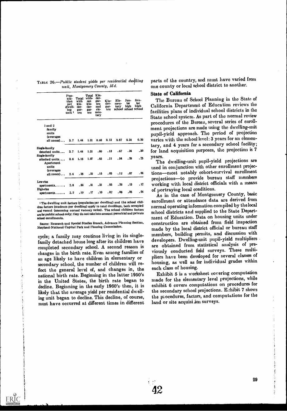
TAnix 26.Publie student yields per residential dmillingunit, Montgomery County, Md.
Pop- Total Kin-ula- Total with- der-lion with out gar- Kin-per kin- kin- ten der-
dwell- der- der- and gor-ing gar- gar- ele- ten
unit I ten ten men-tory
Eie- Jun- Sen.men- lot' fortory high high
school school school
1 and 2familyunits(averagesall zones) 3. 7 1, 44 1. 31 O. 80 O. 13 0. 67 O. 34 O. 30
Single-familydetached units 3. 7 1. 44 1. 31 80 13 67 . 34 30
Single-familyattached units 3. 6 1. 18 1. 07 . 65 . 11 54 25
Apart mentunits(averagesall zones) 2. 4 . . 25 . 15 .03 12 .07 .06
Low-risoapartments . 50 . . 31 .05 . 26 . 13 . 12
Righ-risoapartments " .19 .17 .10 . 02 . OS .05 . 04
I The dwelling unit factors (population per dwelling) and the school chil-dren factors (students per dwelling) apply to total dwellings, both occupiedand vacant (assuming normal vacancy ratios). The school children factorsare for public school only: they do not take into account parochial and private
school enrollments.
Source: Research and Special Studies Branch, Advance Planning Section,Maryland-National Capital Park and Nanning Commission.
cycle; a family may continue living in its single-family detached house long after its children havecompleted secondary school. A second reason ischanges in the birth rate. Even among families ofan age likely to have children in elementary orsecondary school, the number of children will re-flect the general level of, and changes in, thenational birth rate. Beginning in the latter 1950'sin the United States, the birth rate began todecline. Beginning in the early 1960's then, it islikely that the average yield per residential dwell-ing unit began to decline. This decline, of course,must have occurred at different times in different
parts of the country, and must have varied fromone county or local school district to another.
State of CaliforniaThe Bureau of School Planning in the State of
California Department of Education reviews thefacilities plans of individual school districts in theState school system. As part of the normal reviewprocedures of the Bureau, several series of enroll-ment projections are made using the dwelling-unitpupil-yield approach. The period of projectionvaries with the school level: 3 years for an elemen-
tary, and 4 years for a secondary school facility;for land acquisition purposes, the projection is 7years.
The dwelling-unit pupil-yield projections areused in conjunction with other enrollment projec-tionsmost notably cohort-survival enrollmentprojectionsto provide bureau staff membersworking with local district officials with a meansof portraying local conditions.
As in the case of Montgomery County, basicenrollment or attendance data are derived fromnormal operating information compiled by the localschool districts and supplied to the State Depart-ment of Education. Data on housing units underconstruction are obtained from field inspectionmade by the local district official or bureau staffmembers, building permits, and discussion withdevelopers. Dwelling-unit pupil-yield multipliersare obtained from statistical analysis of pre-viously conducted field surveys. These multi-pliers have been developed for several classes ofhousing, as well as for individual grades withineach class of housing.
Exhibit 5 is a worksheet covering computationmade for the elementary level projections, whileexhibit 6 covers computations on procedures forthe secondary school projections. E.Nbit 7 showsthe piocedures, factors, and computations for theland or site acquisilon surveys.
4229
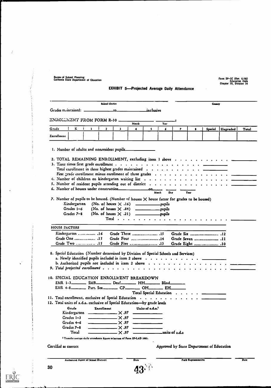
Bureau of School PlanningCalifornia State Department of Education
EXHIBIT 5Projected Average Daily Attendance
Grades m.,in tained
School district
CO ;nclusive
ZNIIOLLMINT FROM FORM R-30Month Yen.
Form SP-1E (Rev. 6/66)Education Code
Chapter 10. Division 14
Grade K i 2 I 4 5 6 7 8 Smili_ Ungraded Torsi
Ear* Ilmoac
1. Number of adults and nonresident pupile
2. TOTAL REMAINING ENROLLMENT, excluding item 1 above3. Three times first grade enrollment
Total enrollment in three highest grades maintainedFirst grade enrollment minus enrollment of three grades
4. Number of children on kindergarten waiting listS. Number of resident pupils attending out of district6. Number of houscs under construction on
Month Day Yam
7. Number of pupils to be housed. (Number nf houses X house factor for grades to be housed)Kindergarten (No. of houses X .16) pupilsGrades 1-6 (No. of houses X .84) pupilsGrades 7-8 (No. of houses X .21 ) pupils
Total
HOUSE 17AGTORS
Kindergarten .16 Grade Three .15 Grade Six .12Grade One .15 Grade Four 14 Grade Seven .....--.... .11Grade Two .15 Grade Five .13 Grade Eight ........... ........ ..... .10
8. Special Education (Number determined by Division of Special Schools and Services)a. Newly identified pupils included in item 2 aboveb. Authorized pupils not included in item 2 above
9. Total projected enrollment
1
10. SPECIAL EDUCATION ENROLLMENT BREAKDOWNEMIt 1-3 SMR-- Deaf HH Blind__
v
EMIt 4-8 Part. See.-- CP 014___ Eli_Total Special Education
I
1
11. Total enrollment, exclusive of Special Education
1
12. Total units of a.d.a. exclusive of Special Educationby grade levelsi Grade Inrollmont Unica of a.d.a.'f
Kindergarten X .97Grades 1-3 X .97Grades 4-6 X .97Grades 7-8 X .97
Total X .97 units of a.d.aI 'imam daily attendance fiounts to bottom of Form 5P4.AD 1003.
Certified as correct Approved by State Department of Education
30
Autttortmo Agent el School District Data Fiold Roprmoototivit Dam
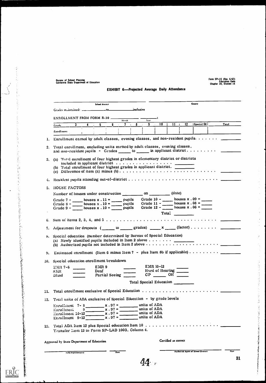
1.
2.
3.
4.
5.
6.
7.
s.
P.
0.)'6-
il.[-i-c.
10.
..,f.,z.r1/4:
t,t.'I.:.
11.
ii. 12.
13.
-
Bureau of School PlanningCalifornia State Depadment of Education
EXHIBIT 6Projected Average Daily Attendance
Graii.cs rm,iiitaincd
form SP-1S (Rev. 6/67)Education Code
Chapter 10, Division 14
School thassics Gooey
to inclusive
ENROLLMENT FROM FORM R-30Slooth Scat
rale 3 4 , 5 6 7 8 9 10 I 11 I 12
EnrollmentI I 1
Special Ed.I Total
Enrollment earned by adult classes, evening classes, and non-resident pupils
Total enrollment, excluding units earned by adult classes, evening classes,and non-resident pupils - Grades lo in applicant district
(a) Tot.l.t enrollment of four highest grades in elementary district or districtsincluded in applicant district
(b) Tot;t1 enrollment of four highest grades in applicant district(c) Difference of item (a) minus (b)
Resident pupils attending out-of-district
HOUSE FACTORS
Number of houses under construction . on (date)
Grade 7 - houses x . 11 = pupils Grade 10 - houses x .09 =Grade 8 - houses x . 10 = pupils Grade 11 - houses x .08 =Grade 9 - houses x . 10 = pupils Grade 12 - houses x .06 =
Total
Sum of items 2, 3, 4, and 5
Adjustment. for dropouts ( to grades) x (factor)
Special education (number determined by Bureau of Special Education)(a) Newly identified pupils included in Item 2 above(b) Authorized pupils not included in Item 2 above .
Estimated enrollment (Item 6 minus Item 7 - plus Item 8b if applicable)
Special education enrollment breakdown
EMR 7-6 EMI1 9 EMI1 10-12SN'ill Deaf Hard of HearingBlind Partial Seeing CP OH
Total Special Education
Total enrollment exclusive of Special Education
Total units of ADA exclusive of Special Education - by grade levels
Enrollment 7- S x . 97 = units of ADA1,.aroi1mer.t 9 x . 97 = units of ADAEnrollment 10-12 x . 97 = units of ADAEnrollment 9-12 x . 97 = units of ADA
Total ADA Item 12 plus Special education Item 10Transfer :tem 13 to Form SP-LAD 1003. Column 4
Approved by State Department of Education Certified as correct
I NW Itervioeft Date Astlowool Antos of School I)
44.81
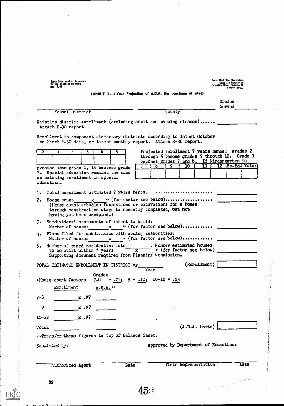
I
State Deputment of EducationBureau of School PlanningRev. 8/61
EXHIBIT 7-7-Year Projection of A.D.A. (for purchase of sites)
Salanistriet
Foim SP-1 Site (Secondary)State Aid Chapter 10
Education Code. Division 14Section 19577
County
Existing district enrollment (excluding adult and evening classes)Attach R-30 report.
Enrollment in component elementary districts according to latest Octoberor Narch R-30 data, or latest monthly report. Attach R-30 report.
X 7-77-12---,
3
1
I
1
.c
i
grewter than grade 1, it becoMed grade7. Special education remains the sameas existing enrollment in specialeducation.
GradesServed
Projected enrollment 7 years hence: grades 2through 5 become grades 9 through 12. Grade Ibecomes grades 7 and 8. If kindergarten is
0 1Sp.Ed .11!OTZ)
1. Total enrollment estimated 7 years hence
2. House ccunt x * (for factor see below)(House count embodrgrroundations or excavations for a housethrough construction stage to recently completed, but nothaving yet been occupied.)
3. Subdivider& statements of intent to build:Number of houses x * (for factor see below)
4. Plans filed for subdivision with zoning authorities:Number of houses * (for factor see below)
5. Number of zoned residentfal lots Nugoer estimated housesto be built within 7 years x * (for factor see below)Supporting document required from PliVigii-Commission.
TOTAL ESTIMATED ENROLLMENT IN DISTRICT byYear
Grades*House count factors: 7-8 = .21; 9 = .10; 10-12 = .23
Enrollment
7-3 x .97
9 x .97
10-12 x .97
Total =1/I
**Transfer these figures to top of Balance Sheet.
(Enrollment)
(A.D.A. Units)
Subaitted by: Approved by Department of Education:
Luthorized Agent
32
Date Field RepresentativePI=NIM,0
Date
CHAPTER 5
LONGRUN PROJECTION TECHNIQUES: INTEGRATEDSTATE AND LOCAL AREA SCHOOL ENROLLMENT
The previous chapters described some of theproblems confronting school planners in the areaof enrollments projection, analyzed trends in theform of administrative organization of the schoolsystems in the United States, and described cur-rently used short-range enrollment projection tech-niques. In this chapter the reader is introducedto the concept of long-range school enrollmentprojections used throughout the balance of thisreport. The general structure of the integratedState-local area school enrollment projection tech-nique will be discussed, and the detailed mechanicsof the approach will be shown in the followingchapters.
State and Local Area Projection TechniqueThe Concept
The general approach consists of first makingprojections of public school enrollment for theState, and then working from the State downwardto the county and local school district. In this waythe local unit is fitted into the framework of thelarger geographic area, and full advantage takenof all available knowledge regarding possible futurepopulation movements. In this respect our ap-proach is somewhat analogous to that used by theU.S. Census Bureau in making population esti-mates for metropolitan areas. The Census Bureaucommented as follows:
In the present report, however, since estimates havebeen developed for all metropolitan areas and for thenonmetropolitan remainders of the States, it was possibleto take advantage of the availability of independent Statetotals developed as part of the Census Bureau's regularestimates program. The independent State figures arebelieved to have a much higher degree of accuracy thanestimates of subareas of States. Adjustments to Statetotals should provide, therefore, an improvement in esti-mates for individual areas, on the average. Consequently,the estimates for metropolitan areas and nonmetropolitanparts of each State were slimmed and adjusted to State
totals. (Quoted from: Population Estimates, Series P-25,No. 371, August 14, 1967, p. 11.)
Underlying this concept is the knowledge thatalmst all children between the ages of perhaps5 and 17 are enrolled in elementary or secondaryschool. Hence, the first major job in making aschool enrollment projection is that of making apopulation projection for children and teenagers;at this point, school enrollment projections arebarely different front population projections. How-ever, the large majority, but not all, of the childrenare enrolled in public schools. This fact calls foradditional techniques in order to project enroll-ment in public schools; on the other hand, thefact that so large a proportion is in public schoolmakes the projection job relatively easy, once thepopulation projection has been made.
Because of the foregoing, the integrated pro-jection is meant to be used for long-range projec-tions, beyond 5 to 10 years. In effect, it is to beused for a time period well beyond the limits oflocally generated vital statistics data, grade-to-grade survival patterns, and dwelling-unit multi-pliers. Indeed there is no need to use this methodfor shortrun projections since previous empiricalevidence has shown that both the dwelling-unitpupil-yield approach and the grade-survivalmethods are fairly accurate for the shortrun timeperiods.
Advantages of this TechniqueThe advantages of the integrated State and
local area school enrollment projection techniquemay be summarized as follows: First, a range ofenrollment projections rather than single esti-mates for future enrollments can be generated.This is accomplished (1) through the introductionof alternate series of population projections forthe State, based on different assumptions ofpopulation growth; and (2) the introduction of
33
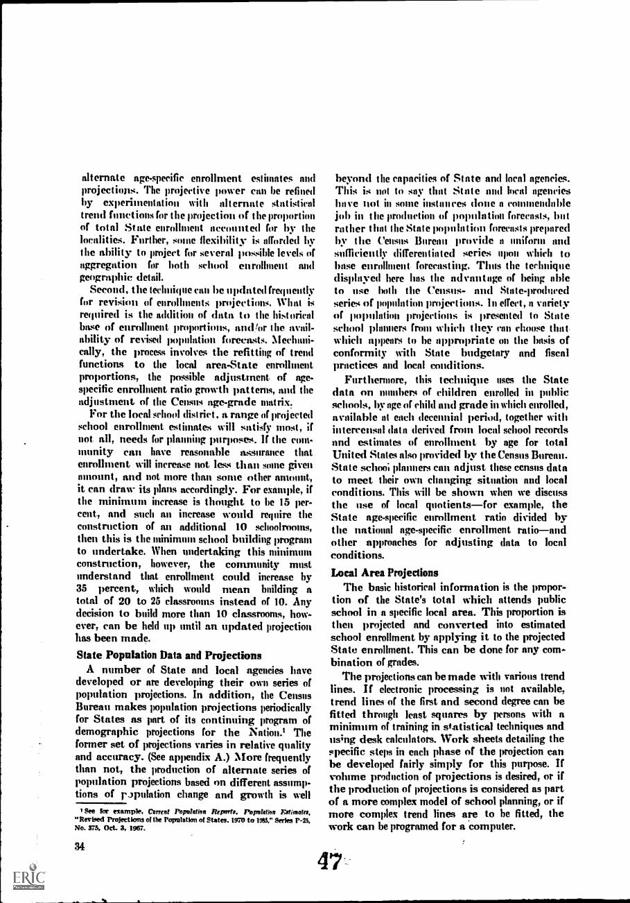
alternate age-specific enrollment estimates andprojections. The projective power can be refilledby experhnentation with alternate statisticaltrend fnnctions for the projection of the proportionof total State enrollment accounted for by thelocalities. Further, some flexibility is afforded bythe ability to project for several possible levels ofaggregation for both school enrollment andgeographic detail.
Second, the technique can be updated frequentlyfor revision of enrollments projections. Wlmt isrequired is the athfition of data to the historicalbase of enrollment proportions, and/or the avail-ability of revised population forecasts. Mechani-cally, the process involves the refitting of trendfunctions to the local area-State enrollmentproportions, the possible adjustment of age-specific enrollment ratio growth patterns, and theadjustment of the Census age-grade matrix.
For the local school district, a range of projectedschool enrollment estimates will satisfy most, ifnot all, needs for planning purpose4. If the com-munity can have reasonable as.surance thatenrollment will increase not less than some givenamount, and not more than some other amount,it can draw its plans accordingly. For example, ifthe minimum increase is thought to be 15 per-cent, and such an increase would require theconstruction of an additional 10 schoolrooms,then this is the minimmn school building programto undertake. When undertaking this minimumconstruction, however, the community mustunderstand that enrollment could increase by35 percent, which would mean building atotal of 20 to 25 classrooms instead of 10. Anydecision to build more than 10 classrooms, how-ever, can be held up until an updated projectionhas been made.
State Population Data and ProjectionsA number of State and local agencies have
developed or are developing their own series ofpopulation projections. In addition, the CensusBureau makes population projections periodicallyfor States as part of its continuing program ofdemographic projections for the Nation.' Theformer set of projections varies in relative qualityand accuracy. (See appendix A.) More frequentlythan not, the production of alternate series ofpopulation projections based on different assump-tions of rmulation change and growth is well
see for example. Montt PopuhtMn Report*, Population Estimates."necked Projections oi the Population oi States. 1970 to 1955," Series P-15,No. 375, Oct. 3, 1967.
34
beyond the capacities of State and local agencies.This is not to say that State and local agencieshave not in some instances done a commendablejob in the prodnetion of population forecasts, butrather that the State population forecasts preparedby the Census Bureau provide a uniform andsufficiently differentiated series upon which tobase enrollment forecasting. Thus the techniquedisplayed here has the advantage of being ableto use both the Census- and State-producedseries of population projections. I II effect, a varietyof population projections is presented to Stateschool planners from which they can choose thatwhich appears to be appropriate on the basis ofconformity with State budgetary and fiscalpractices and local conditions.
Furthermore, this technique uses the Statedata on numbers of children enrolled in publicschools, by age of child and grade in which enrolled,available at each decennial period, together withintercensal data derived from local school recordsand estimatm of enrollment by age for totalUnited States also provided by the Censns Bureau.State schooi planners can adjust these census datato meet their own changing situation and localconditions. This will be shown when we discussthe use of local quotientsfor example, theState age-specific enrollment ratio divided bythe national age-specific enrollment ratioandother approaches for adjusting data to localconditions.
Local Area ProjectionsThe basic historical information is the propor-
tion of the State's total which attends publicschool in a specific local area. This proportion isthen projected and converted into estimatedschool enrollment by applying it to the projectedState enrollment. This can be done for any com-bination of grades.
The projections can be made with various trendlines. If electronic processing is not available,trend lines of the first and second degree can befitted through least squares by persons with aminimum of training in statistical techniqnes andus;ng desk calculators. Work sheets detailing thespecific steps in each phase of the projection canhe developed fairly simply for this purpose. Ifvolume production of projections is desired, or ifthe production of projections is considered as partof a more complex model of school planning, or ifmore complex trend lines are to be fitted, thework can be programed for a computer.
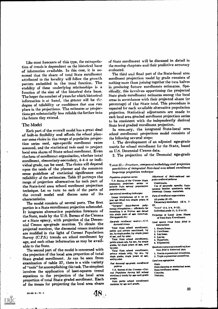
Like most forecasts of this type, the extrapola-tion of trends is dependent on the historical baseof information available. In this case, it is as-sumed that the share of total State enrollmentattributed to the locality will follow the growthpattern embedded in the trend function. Thestability of these underlying relationships is afunction of the size of the historical data base.The larger the number of years for which historicalinformation is at hand, the greater will be thr.degree of reliability or confidence that one canplace in the projections. The estimates or projec-tions get substantially less reliable the farther intothe future they extend.
The ModelEach part of the overall model has a great deal
of built-in flexibility and affords the school plan-ner some choice in the range of population projec-tion series used, age-specific enrollment ratesassumed, and the statistical tools used to projectlocal area shares of State school enrollment. Eventhe form of enrollment organization, whether totalenrollment, elementary-secondary, 4-4-4 or indi-vidual grade, can be used. The choice will dependupon the needs of the planner and the commonsense guidelines of statistical significance andreliability of the estimates. Table 27 portrays therange of projection alternatives for each part ofthe State-local area school enrollment projectiontechnique. Let us turn to each of the parts ofthe overall model and discuss some of itscharacteristics.
The model consists of several parts. The firstportion is a State enrollment projection submodel.It integrates alternative population forecasts ofthe State, made by the U.S. Bureau of the Censusor a State agency, with projection of the Decen-nial Census age-grade matrices. To obtain theprojected matrices, the decennial census matricesare modified in the light of Current PopulationSurvey (C.P.S.) trends on school enrollment byage, and such other information as may be avail-able to the State.
The second part of the model is concerned withthe projection of the local area proportion of totalState graded enrollment. As can be seen fromexamination of table 27, there is a wide varietyof "tools" for accomplishing this task. The simplestinvolves the application of least-squares trendequations to the projection of the local areaproportion of total State graded enrollment. Eachof the means for projecting the local area share
353-511 0 - 7o - 4 48
of State enrollment will be discussed in detail inthe ensuing cluipters and their predictive accuracyevaluated.
The third and final part of the State-local areaenrollment projection model by grade consists ofnothing more than joining together the two halvesin producing future enrollments estimates. Spe-cifically, this involves apportioning the projectedState grade enrollment estimates among the localareas in accordance with their projected share (orpercentage) of the State total. This procedure is
repeated for each available alternative populationprojection. Statistical adjustments are made toeach local area, graded enrollment projection seriesto be consistent with the independently derivedState level graded enrollment projection.
In sumfaary, the integrated State-local areaschool enrollment. projections model consists of
the following several steps:I. The development of an adjusted age-grade
matrix for school enrollment for the State, basedon U.& Decennial Census data.
2. The projection of the Decennial age-grade
TATILE 27. Structure, component methodology and projectionpossibilities of integrated State-local arca school enrollmentloug.ratage projection technique
Population projection series
U.S. Boman of the Census Statepopulation prolectkm series orsuitable State agency populationpro)ect ion scrim.
Age-taterral transtlieg techniqueLinear intetpolation of 5- or In-
year age detail into single years ofage intervals.
"Sprague" thinl-degrre poly-nomial interpolatkm e efficient, forsmoothing 5- or 10-year see detailinto single years of age intervals.(See append it IL)
Aft-orade enrcUment matrirU.S.iferennial crises
Total State school enrollment,public and private combined. byset, by single grades, by single yearsof age, and by color.
Total State school enrollment,public school may, by sex, by singlegrades, by single years of age, andby color.
Total State school enrollment,private schools only, by sex, bysingle gradm, single years of age,and by color.
Pali decennial ar-frade enrollment',Mons
U.S. Bureau of the CensusCat-reef Population San-re fall schoolenrollmeat trends hy age and gradegroups.
State public school enrollmentstatistks by age and grade.
ilifjeafaref of SIMSe-natkad ape-gook coral/meg patterns
Guestimates.Use of age-grade specific State-
national location quotients usingDecennbi Census materials.
Porm of enrollment °maxi-Wien
AB grades (K-12).Elementary-secondary (K4, 2-
12)."4 44" (1-4, 5-6, 9-17).Individual grade (1, 2, 3 to 12).
Pnjection of Local Ares Sharesof Total State Enrollment
Least serous tread lines fated tohistoricellaM
I. Simple linear.2. Curvilinear.3. Log linear.4. Log log.5. Hyperbolic.6. Exponential.
fivadroticerposential smoothing fan-lions fitted to historical dato
1. Double exponential smoothing.2. Triple exponential smoothing.
Loot/area aserreattonState.State planning or statistical areas.State enrollment areas.Counties.Districts.
35
matrix for the State using suitable adjusted growthrates in specific age-grade grouping enrollmentcells derived from the U.S. Census C.P.S. statis-tical series on fall school enrollments, as well asother locally available information.
3. Application of projected age-grade matrix forthe State to detailed age-projections of its popu-lation to derive estimated enrollment by gradegroup. These serve as controls for the local politicalunit projections, derived as follows:
4. The fitting of statistical trend functions tolocal political unit-State enrollment ratios.
5. The projection of local political unit-Stateenrollment ratios through interpolation of sta-tistical trend functions derived in step 4.
6. Application of projected local political unit-State enrollment ratios, derived in step 4, toobtain estimated detailed enrollments.
7. Adjustment of detailed enrollment estimatesderived in step 6 to overall State estimatesobtained in step 3.
36
49
The next two chapters deal with the detaileddescription of the development of the integratedState-local projection model.
Chapter 6 considers the development, of Statelevel graded enrollment projections. Material cov-ered includes development and modification ofDecennial Census age-grade enrollment matricesand application to State projections of the school-age population. Examples and work sheets areshown for each step in the computations. TheStates of California and Maryland serve as test.cases for this phase of the approach and remainingtechnical chapters.
Chapter 7 shows the development and projec-tion of local area proportions of total Stateenrollment. A variety of statistical trend tech-niques are discussed and applied to data on enroll-ment by State Statistical Area for California andcounty for Maryland. These projected shares arethen applied to the projected State enrollment toarrive at projected local area enrollment.
CHAPTER 6
DEVELOPMENT OFSTATEWIDE ENROLLMENT PROJECTIONS
This chapter covers the first portion of theintegrated State-local area enrollment projectionoutlined in chapter 5. In particular, the followingprocedures in making the statewide enrollmentforecasts are discussed.
I. Development of State-level age-grade specificenrollment ratios for use in making statewideprojections.
2. Modification and projection of statewideage-grade specific enrollment ratios for use inconjunction with population projections for theState.
3. Application of statewide projected age-gradeenrollment ratios to statewide population pro-jections by age to derive final estimates of futureschool enrollment.
The relative accuracy of this approach will beevaluated, using some comparison with actualenrollment data. Further, possible modificationsof the approach in the light of trends in publicand private school enrollment will be discussed.For the interest of the user, work tables depictingstep-by-step computations will be displayed.
Projections by sex ' and color are possibleinsofar as the basic decennial census data containsthis information. However, as will be pointed outin chapter 7, historical data on public schoolenrollment must also be available by sex andcolor in order to make such enrollment projections.In addition, projected population data by age andcolor are needed. The Census Bureau, however,provides projected age by color estimates only forStates which had 250,000 or more nonwhitepopulation in 1960. Accordingly, before attemptingany enrollment projections by color, the Statetechnician should ascertain from the CensusBureau whether he can obtain the data neededfor his target date.
I As a Practical measum there is probably little value in making projectionstor boys and girls separately. so that the set dichotomy can be ignored.
59
Population and school enrollment data for thisand the succeeding chapters covering the pro-cedures in the integrated State-local level schoolenrollment projection approach are for the Statesof Maryland and California. School enrollmentforemsts cover the period from 1965 to 1985.The results are shown at 5-year intervals. Theform of school enrollment used in the illustrationis the 4-4-4 arrangementgrades 1-4, 5-8, and9-12.
Statewide Age-Grade Specific EnrollmentRatios
Age-gradr: specific enrollment matrices will bedeveloped for the 1960 public school populationof Matyland. This table, when adjusted for trendsin certain age-grade cells in the matrices, will beused with Census Bureau population projections,subdivided into single years of age, to makeschool enrollment projections. The modificationof the final ace-grade enrollment tables and their
application to the Census popuiation projectionsby single years of age will be the subject of thenext section.
Basic data for the development of the age-gradeenrollment matrix are obtained from the mostrecent U.S. Census volume on detailed charac-teristics of the population in each State; forexample, Series PC(1)-D in 1960. The specific
tables used in constructing the 1960 matrix are:(1) "Year of School in which Enrolled for Persons5- to 34-years-old by Single Years of Age, Color,Sex, and Type of School (Public and Private), forthe State: Urban and Rural: 1960;" (2) "Single
Years of Age, by Color, Nativity, and Sex, for the
State: 1960."Age-grade data on school enrollments for 1960
are shown for each sex separately and for all
37
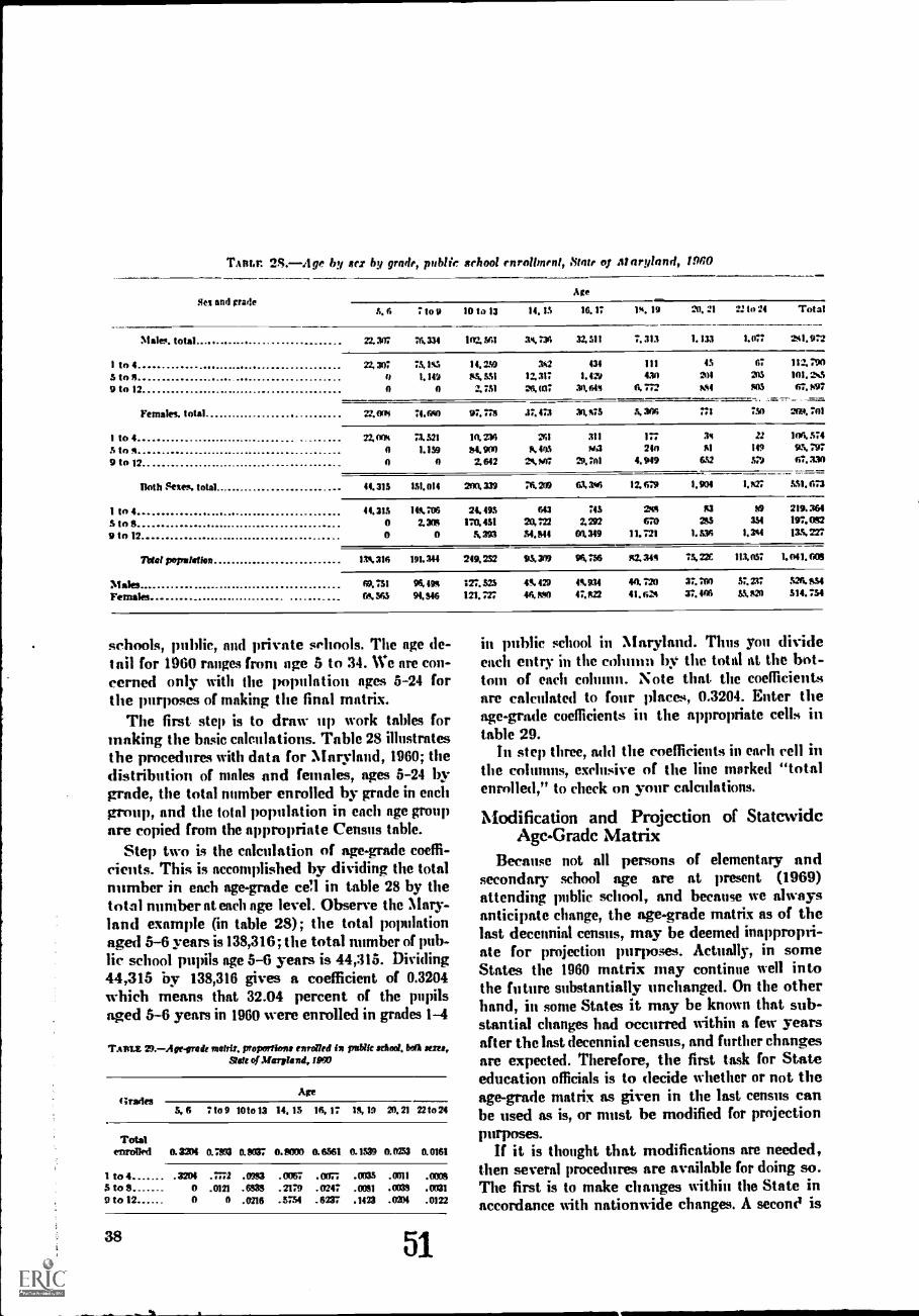
TAMA: 28.-Age by sex by gentle, public school enrollment, Stnte oy ;nary land, 1960
Ses and gradeAge
5.6 :toy 10 to 13 14. IS 16. 17 ls. 19 20. 21 72 10 24 Total
Malec total 22.307 76,334 102. 361 35.734 32.511 7. 31:1 1.133 1.077 291.972
1 to 4 n, 307 73. 1%5 14.259 3s2 434 111 IS 07 112,790
5 to 11 0 1.149 93, 331 12.317 1.429 430 201 205 101. 2s3
9 to 12 0 0 2. 751 26, I K 47 30. 619 6, 772 MI 505 67, 597
Females. total 22, OW 74.W o 92.775 37.473 311,143 S. 306 771 750 2M, 701
I to 4 22, nes 73.321 10,216 261 311 177 3s 22 106,574
to 0 1.139 64.900 5.405 963 210 SI 119 95. 797
9 to 12 0 0 2.642 25.907 29.701 4. 949 652 379 67.330
Both Seses. total 41.313 131.014 200. 339 76.209 62. 3,40 12. 679 1. 901 1.527-
331.073
1 to 4 41.313 145.706 24,495 613 745 WS 93 59 219. 364
to S 0 2.314 170,431 20.722 2.292 670 295 331 197.092
9 to 12 0 0 5,393 51.541 00, 349 11.721 I. 334 1.344 135.227
Meal peps/dim: 1:91.316 191.344 249,252 95. 309 96,756 92. 345 73,22t 115.037 1.041. 609
Males 69.731 96,195 127.5n 49.479 45. M4 40. 720 at 700 57.217 326. S34
Females CA, 505 91,946 121.727 46,550 47.622 41.629 37.406 53.920 514.754
schools, public, and private schools. The age de-tail for 1960 ranges from age 5 to 34. We are con-cerned only with the population ages 5-24 forthe purposes of making the final matrix.
The first step is to draw up work tables formaking the basic calculations. Table 28 illustratesthe procedures with data for Maryland, 1960; thedistribution of males and females, ages 5-24 bygrade, the total number enrolled by grade in eachgroup, and the total population in each age groupare copied from the appropriate Census table.
Step two is the calculation of age-grade coeffi-cients. This is accomplished by dividing the totalnumber in each age-grade cell in table 28 by thetotal number at each age level. Observe the Mary-land example (in table 28); the total populationaged 5-6 years is 138,316; the total number of pub-lic school pupils age 5-6 years is 44,315. Dividing44,315 by 138,316 gives a coefficient of 0.3204which means that 32.04 percent of the pupilsaged 5-6 years in 1960 were enrolled in grades 1-4
Tan= 29.-Apeirade nefrir. proportions enrolled in put& school. baik seru,sale of Maryland, 1960
t ;raftsAge
5, 6 :to 9 10 to 13 14. 15 16, 17 15, 19 20. 21 22 to 24
Totalenrolled 0.3204 0.7103 0.9017 0.9000 0.6561 0.1539 0.0253 0.0161
1 to 4_ ..... .3204 .7772 .0993 .0067 . cm= .0035 .0911 .0009to 9 0 .0121 .6939 .2179 .0247 .0091 .0039 .0)31
9 to 12 0 0 .0216 .5754 .6237 .1423 .0204 .0122
38 51
in public school in Maryland. Thus you divideeach entry in the colmnn by the total at the bot-tom of each column. Note that the coefficientsare calculated to four places, 0.3204. Enter theage-grade coefficients in the appropriate cells intable 29.
In step three, add the coefficients in each cell inthe columns, exclusive of the line marked "totalenrolled," to check on your calculations.
Modification and Projection of StatewideAge-Grade Matrix
Because not all persons of elementary andsecondary school age are at present (1969)attending public school, and because we alwaysanticipate change, the age-grade matrix as of thelast decennial census, may be deemed inappropri-ate for projection purposes. Actually, in someStates the 1960 matrix may continue well intothe future substantially unchanged. On the otherhand, in some States it may be known that sub-stantial changes had occurred within a few yearsafter the last decennial census, and further chancesare expected. Therefore, the first task for Stateeducation officials is to decide whether or not theage-grade matrix as given in the last census canbe used as is, or must be modified for projectionpurposes.
If i t is thought that modifications are needed,then several procedures are available for doing so.The first is to make changes within the State inaccordance with nationwide changes. A seam' is
to adopt the matrix (from (he last DeceimialCensus) for some other State which can be iised a.sa model. A third alttrnative is for the State totabulate its own records, age by grade, and usethis information for changing the last DecennialCensas matrix. Finally, State officials may simplyassmne smne model age-grnde matrix which theyexpect to achieve by the time of the target date.
Note that at this judgment of State andlona co»ditions becoLies imporl ant in estimatinga future age-grade ina'rix for pnblic schools. Forexample, in 1060 in Mlryland, among 5- and 6-year-olds, 0.3204 were (limited in public schools;in California the figure wa.s 0.3461 and for totalUnited States, 0.3076. There is no guaranteedstatistical procedure for estimating what thisratio, 0.3204, will be in Maryland in 1980. Willit continne to be above the national average? Willit equal California's ratio of 0.3461? Or will it besome other value? Jmigment about local conditionsis the best gni(le.
In the following materials we are focusing ourattention on the use of nationwide changes toindicate changes within the State. The last threealternatives require no additional technical ex-planations; the mechanics for carrying them out.are similar to those for the first alternative.
Two sets of procedures for projecting the age-grade matrix using nationwide changes are shown.The first set is recommended. The second set isincluded to show a possible alternative way ofprojecting the matrix; dne to lark of snfficientinformation, however, it is probable that fewStates will be able to apply this second set ofprocedures. Nevertheless, some States may beable to use this second set, or some adaptation ofit, depending on the data which may be locallyavailable.
First Set of ProceduresIn the following illustration for Maryland, we
have made the basic assumption that the 1980goal for the State will be the national average asof 1960; the only exception is the 5- and 6-yearage gronp which, in 1960, was already above thenational average. For California., which wasalready above the national average in 1960, weassumed no further changes. In reality, theseassumptions need not hold for either of these twoStates or any other State; State officials must,decide for themselves what the appropriate goalsmay be. Whatever goals are mused, however, themechanics to be followed in extrapolating the last
52
_
Decennial Census matrix are exactly the same asillustrated in the following pages. In case of &Aias to which standard is the most appropriate, twoor more 11:ternative ones may he used and a rangeof estimated chn,iges calculated.
Two steps are involved in this procedure. First,State-national location quotients, as of the time of
the most recent censns, mast be calculated foreach total-age enrollment gronp. This is necessaryto ascertain the degree of adjustment to be madein the projection of specific age-grade enrollmentratios. Second, the basic matrix tnay be pmjectedusing the State-national total-age enrolhnentgroup location quotient computed in the first step.
The first step in the adjustment of the age-grade matrix, the development of the State-national age enrollment location quotient, is fairlysimple. Table 30 displays the necessary computa-tions for Maryland and California. Cohnun ashows for total United States, the proportionenrolled in each age group. Column b contains thesame proportions computed for 1960 public schoolenrollment for Maryland as given in table 29. Bydividing each of the entries in column a by therespective entries iii column b, we obtain theratios shown in column c. These ratios are theState-national enrollment-location quotients men-tioned previously. They reflect the degree to which
the State public school age-enrollment patternsare either greater or smaller than the 1960 nationalpublic school age-enrollment levels.
If the proportion in a given age group in a Statehas a ratio below 1.0 as shown in column c, oftable 30, then the State has a larger proportionenrolled than does the Nation. Just the opposite is
(me for those ages with age-enrollment ratiosgreater than one, or unity. in these ages, the pro-portions enrolled are below prevailing nationalage-enrollment levels.
The reader is warned that these age-enrollmentadjustment factors should not be applied me-chanically. State education planners should beknowledgable about local conditions and gradedenrollment trends. Thus, the adjustment factorsshould be further manipulated by State plannersto reflect sudden changes in, for example, the dis-tribution or the total school enrollment populationbetween public and private systems; such a factorcannot be treated mechanically. Thus, good com-mon sense and judgment must be employed in theuse and application of the State-national age-enrollment adjustment factors.
For the projections of the Maryland and Cali-
a39
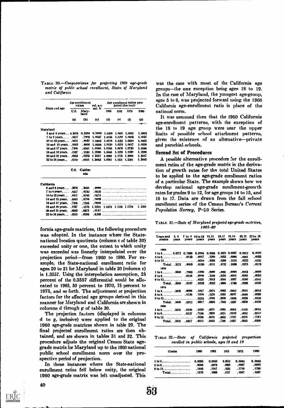
TABLE 30.-Compu lotions for projecting 1960 age-gradematrix of public school enrollment, Staks of Marylandand Californht
State cnd age
Age enrollmentrst los col. a+
b
Are enmllment ratios pro-jected (See test)
col.U.S. Mary-
land1985 1970 1975 1990
(a) (b) (c) (d) (01 (I) 00
Maryland5 and 6 years- 0 30767 to 9 years A317
10 to 13 years... M1114 and 15 yeats. 6445
16 and 17 years. 7321
IS and 19 years. 1937
20 and 21 years. 0343
22 to 24 years.. 0210
0.3201. 7993.9037.9000.6561.103.0233.0161
0.96001.05371.01151.05561.09801.23861 35571.3043
1.03101.0134
1.01161.01391.02461.06461.09991.0761
1.0401
1. DM1.0232
1.0231.0413
1.1243
1.1779
1.1521
1.06411.0403
1.03491.04171. 0739
1.19391.26661.2281
1.19021.05371.04651.01361.09961.25961.35571.3043
U.S. Cantor-nta
California5 and 6 years. .3176 .3461 .
to 9 years ..... .A317 .8732 .952510 to 13 years__ .8411 .9785 .957414 and 15 years. .9445 .8794 .960316 end 17 years. .7314 .7505 .9694MI and 19 years. .1537 .1576 1.2231 1.0573 1.1148 1.1718 1.2291
20 and 21 years. .0343 .0375 .914722 to 24 years.- .0210 .0256 .9203
fornia age-grade matrices, the following procedurewas adopted. In the instance where the State-national location quotients (column c of table 30)exceeded unity or one, the extent to which unitywas exceeded was linearly interpolated over theprojection period-from 1960 to 1980. For ex-ample, the State-national enrollment ratio forages 20 to 21 for Maryland in table 30 (column c)is 1.3557. Using the interpolation assumption, 25percent of the 0.3557 differential would be allo-cated to 1965, 50 percent to 1970, 75 percent to1975, and so forth. The adjustment or projectionfactors for the affected age groups derived in thismanner for Maryland and California are shown incolumns d through g of table 30.
The projection factors (displayed in columnsd to g, inclusive) were applied to the original1960 age-grade matrices shown in table 29. Thefinal projected enrollment ratios are then ob-tained, and are shown in tables 31 and 32. Thisprocedure adjusts the original Census State age-grade matrix for Maryland up to the 1960 nationalpublic school enrollment norm over the pro-spective period of projection.
In those instances where the State-nationalenrollment ratios fell below unity, the original1960 age-grade matrix was left unadjusted. This
40
was the case with most of the California agegroups-the one exception being ages 18 to 19.In the case of Maryland, the youngt age-group,ages 5 to 6, wa.s projected forward using the 1960California age-enrollment ratio in place of thenat ion al norm.
It was assumed then that the 1960 Californiaage-enrollment patterns, with the exception ofthe 18 to 19 age group were near the upperlimits of possible school attachment patterns,given the existence of an alternative-privateand parochiaLschools.
Second Set of ProceduresA possible alternative procedure for the enroll-
ment ratios of the age-grade matrix is the deriva-tion of growth rates for the total United Statesto be applied to the age-grade enrollment ratiosof a particular State. The example shows how wedevelop national age-grade enrollment-growthrates forgrades 9 to 12, for age groups 14 to 15, and16 to 17. Data are drawn from the fall schoolenrollment series of the Census Bureau's CurrentPopuktion Survey, P-20 Series.
TABLE 31.-State of Maryland projected age-grade metrkes,196.5-80
Years andgrades
5, 6years
7 to 9 10 to 13years years
14,15years
1117years
1919.years
23.21years
22 to 24years
1965
110 4 0.3272 ft 7990 0. 004 0. 0058 0. 0079 0.0037 0.0312 0.00095108 .0173 .6917 .2339 .0253 .0096 .0011 .003391012 0219 .5934 . .1515 .0222 .0131
Total. .3272 .9003 .9130 .8111 .6122 .1639 .0275 .01731070
to 4 3310 .7983 .1006 .0069 .0081 .0040 .0013 .00095108 .0124 .6996 .2240 .0259 .0091 .0045 .arca91012 .0221 .5913 .6544 .1607 .0240 .0141
Total. .3340 .8107 .9223 .6222 .6981 .1738 .0299 .01551973
to 4 3409 .9096 .1017 .0079 .0063 .0912 .0014 .0010510 8 .0126 .nr6 . 211) .0265 .0049 .003891012 . 0224 .5994 .6699 .1699 .0259 .0150
Total. .3409 .9212 .9317 .9334 .7018 .1837 .0333 .01931560
1 to 4 3476 .8190 .1029 .0041 .0095 .0044 .0315 .0010$109 .0127 .7156 .2300 . OM .0102 .0052 .00t3910 12. .0226 .6074 .6652 .1791 .0276 .C151
Total. .3476 .8317 .8411 .8445 .7209 .1937 .0343 .0339
TA aLE 32.-State of California projected proportionenrolled in publk schools, ages 18 and 19
Grades 1960 1963 1970 1975 1990
1 to 4 0.0035 0.0040 0.0042 0.0044 0.00465 tog .0046 .0079 .0093 .0097 .00929 to 12 .1495 .1547 .1132 .1716 .1799
Total .1576 .1666 .1757 .1847 .1937
58
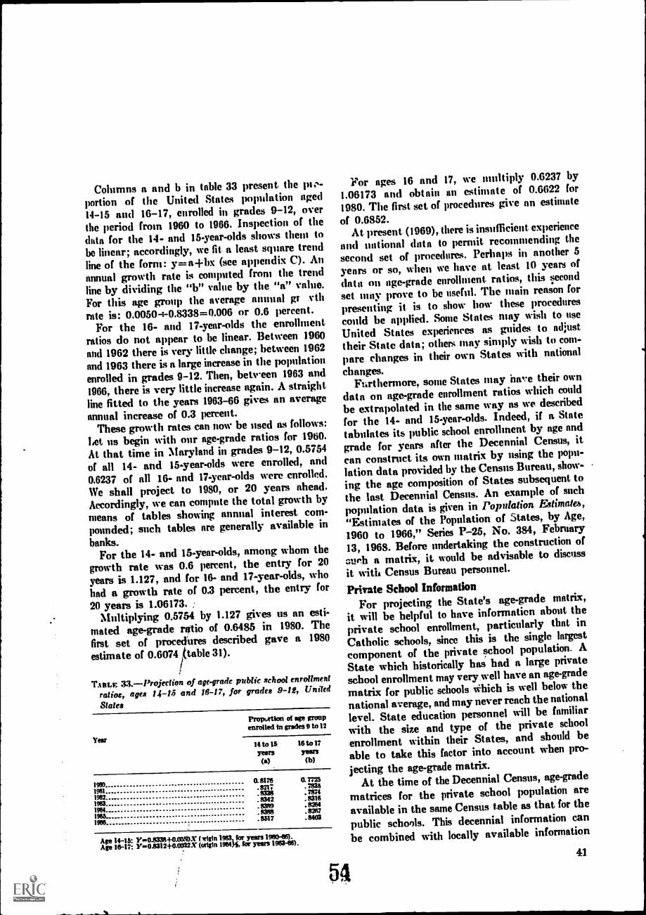
Columns a and h in table 33 present the pt.....portion of tile United States population aged14-15 and 16-17, enrolled in grades 9-12, overthe period from 1960 to 1966. Inspection of the
chart for the 14- and 15-year-olds shows them tobe linear; accordingly, we fit a least square trendline of the form: y---.al-bx (see appendix C). Anannual growth rate is computed from the trendline by dividing the "b" value by the "a" value.For this age group the average annual gt vthrate is: 0.00504-0.8338=0.006 or 0.6 percent.
For the 16- and 17-year-olds the enrollmentratios do not appear to be linear. Between 1960nod 1962 there is very little change; between 1962and 1963 there iff a large increase in the populationenrolled in grades 9-12. Then, between 1963 and1966, there is very little increase again. A straightline fitted to the years 1963-66 gives an averageannual increase of 0.3 percent.
These growth rates can now be used as follows:
Let us begin with our age-grade ratios for 1960.At that time in Maryland in grades 9-12, 0.5754of all 14- and 15-year-olds were enrolled, and0.6237 of all 16- and 17-ycar-olds were enrolled.We shall project to 1980, or 20 years ahead.Accordingly, we can compute the total growth bymeans of tables showing annual interest com-pounded; such tables are generally available in
banks.For the 14- and 15-year-olds, among whom the
growth rate was 0.6 percent, the entry for 20years is 1.127, and for 16- and 17-year-olds, who
had a growth rate of 0.3 percent, the entry for
20 years is 1.06173. :Multiplying 0.5754 by 1.127 gives us an esti-
mated age-grade ratio of 0.6485 in 1980. The
first set of procedures described gave a 1980estimate of 0.6074/(tab1e 31).
TAta.}: M.-Projection of age-grade public school enrollment
ratio:, ages 14-15 and 16-17, for grades 9-12, United
States
Year
Propt,rtlan of age groupenrolled in grades 9 to 12
14 to 15years
(s)
16 to 17Years(b)
190008176 0.7725
1981.8217 . 7835
1962..8338 , 7874
1963.8342 .9316
1904.8389 , 8264
1965..8388 . 8267
1986.8517 .8403
Age 14-15: l'..0.8338-1-0.00.9).Y ('rIgIn 1903. for years 1960-66).Age 16-17: }"=0.8312-1-0.0022X (orIgln 1964)4. for years 1963-66).
54
14'or ages 16 and 17, we multiply 0.6237 by1.06173 and obtain an estimate of 0.6622 for
1980. The first set of procedures give an estimate
of 0.6852.At present (1969), there is insufficient experience
and national data to permit recommending the
second set of procedures. Perhaps in another 5
years or so, when we have at least 10 years of
data on age-grade enrollment ratios, this second
set may pmve to be useful. The Main reason for
presenting it is to show how these procedures
could be applied. Some States may wish to use
United States experiences as guides to adjusttheir State data; others may simply wish to com-
pare changes in their own States with national
changes.Furthermore, some States may imwe their own
data on age-grade enrollment ratios which could
be extrapolated in the same way as we described
for the 14- and 15-year-olds. Indeed, if a State
tabulates its public school enrollment by age and
grade for years after the Decennial Census, it
can construct its own matrix by using the popu-
lation data provided by the Census Bureau, show-
ing the age composition of States subsequent to
the last Decennial Census. An example of such
population data is given in Population Estimatea,
"Estimates of the Population of States, by Age,
1960 to 1966," Series P-25, No. 384, February
13, 1968. Before undertaking the construction of
sueh a matrix, it would be advisable to discuss
it with Census Bureau personnel.
Private School InformationFor projecting the State's age-grade matrix,
it will be helpful to have information about the
private school enrollment, particularly that inCatholic schools, since this is the single largest
component of the private school population. A
State which historically has had a large private
school enrollment may very well have an age-grade
matrix for public schools Which is well below thenational average, and may never reach the national
level. State education personnel will be familiar
with the size and type of the private school
enrollment within their States, and should be
able to take this factor into account when pro-
jecting the age-grade matrix.At the time of the Decennial Census, age-grade
matrices for the private school population areavailable in the same Census table as that for the
public schools. This decennial information can
be combined with locally available information
41
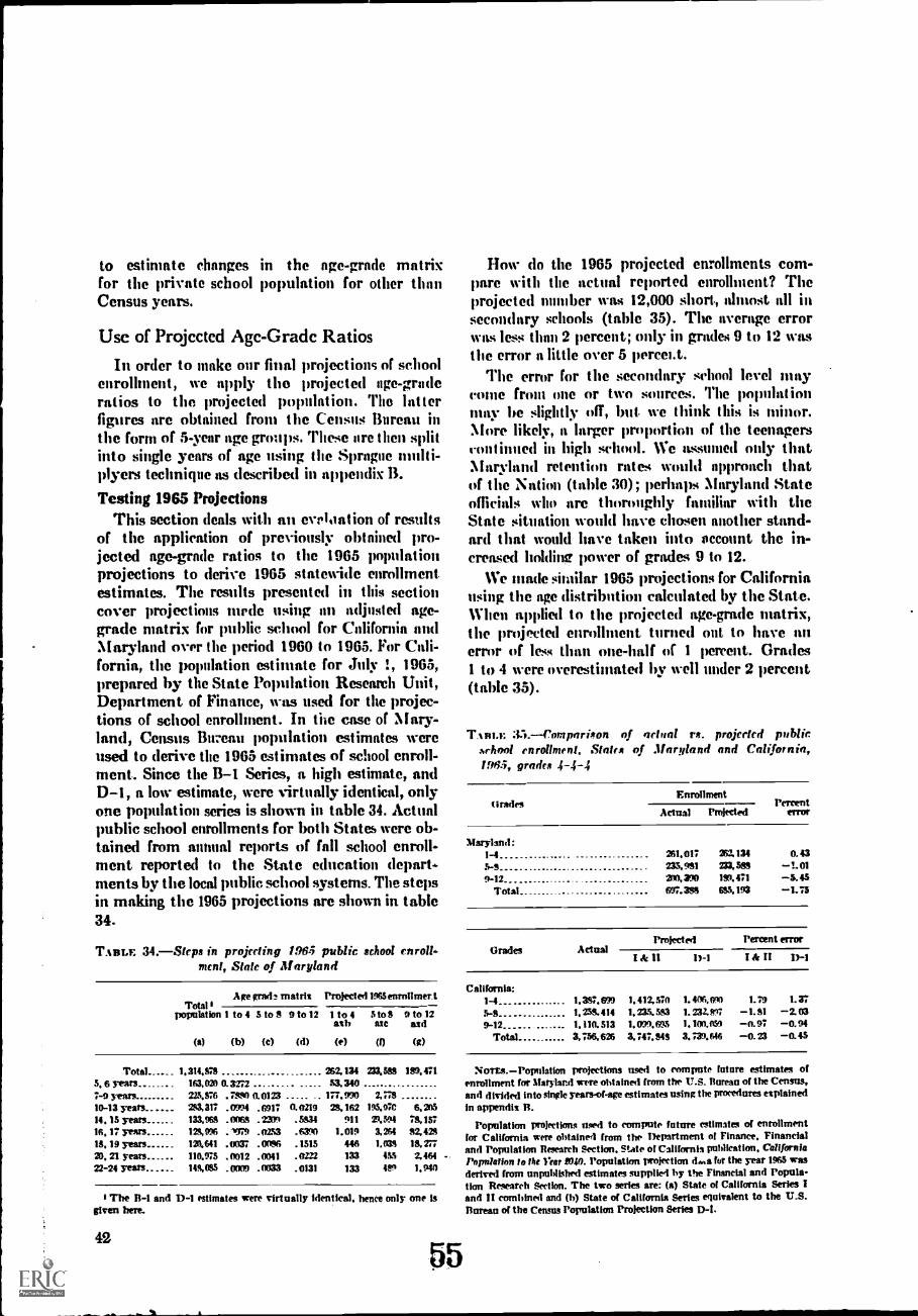
to estinmte changes in the age-grade matrixfor the private school population for other thanCensus years.
Use of Projected Age-Grade Ratios
In order to make our final projections of schoolenrollment, we apply tho projected age-graderatios to the projected population. Tho latterfigures are obtained from the Census Bureau inthe form of 5-year age groups. These are then splitinto single years of age using the Sprague multi-plyers technique as described in appendix II.
Testing 1965 ProjectionsThis section deals with an eveloat ion of results
of the application of previously obtained pro-jected age-grade ratios to the 1965 poimlationprojections to derive 1965 statewide enrollmentestimates. The results presented in this sectioncover projections mrde using an adjusted age-grade matrix for public school for California andMaryland over the period 1960 to 1965. For Cali-fornia, the population estimate for July 1, 1965,prepared by the State Population Research Unit,Department of Finance, was used for the projec-tions of school enrollment. In the case of Mary-land, Census Buzeau population estimates wereused to derive the 1965 estimates of school enroll-ment. Since the B-1 Series, a high estimate, andD-1, a low estimate, were virtually identical, onlyone population series is shown in table 34. Actualpublic school enrollments for both States were ob-tained from annual reports of fall school enroll-ment reported to the State education depart-ments by the local public school systems. The stepsin making the 1965 projections are shown in table34.
TABLE 34.-Steps in projecting 196-5 public school enroll.molt, State of Maryland
Age grad,z. matria Projected 1965 enrollmertTotal
population
(a)
1 to 4 5 to 8 Oro 12
(b) (e) (d)
1 to 4nth
(e)
5 to 8are
(0
9 to 12mut
(g)
Total 1.314.978 262.134 233.588 189.4715, 6 years 163,031 0.3272 53,3407-9 years 229976 .7990 0.0123 177.990 2,77810-13 years 299317 .0394 .6917 0.0219 29, 162 195,07C 6.20514. 15 years 133,969 .0068 .2200 .5934 911 71.594 7915716, 17 years 129096 .1779 .02%3 .6390 1.019 3,264 82,42818, 19 years 131.641 .0037 . OM& .1515 446 1.038 19,27720, 21 years 110.975 .0012 .0041 .0222 133 455 2,46422-24 years 149085 _0009 .0033 .0131 133 499 1.940
1 The I3-1 and D-1 estimates were virtually identical, hence only one isgiven here.
42
How do the 1965 projected enrollments com-pare with the actual reported enrollment? Theprojected number was 12,000 short, almost all insecon(iary schools (table 35). The average errorMIS less than 2 percents; only in grades 9 to 12 wasthe error a little over 5 perceLt.
'Ille error for the secondary school level mayconle from (me or two sources. The populationntay be slightly off, but we think this is minor.More likely, a larger proportion of the teenagers(-Olitinued in high school. We as.sumed only that,NIaryland retmtion rates would approach thatof the Nation (table 30); perhaps Maryland Stateofficials who are thoronghly familiar with theState situation would have chosen another stand-ard that would have taken into occount the in-creased holdine power of grades 9 to 12.
We made similar 1965 projections for Californiausing the age distribution calculated by the State.When applied to the projected age-grade matrix,the projected enrollment turned out to have anerror of less than one-half of 1 percent. Grades1 to 4 were overestimated by well under 2 percent(table 35).
TAMA: 33.-Cornparivon of actual rs. projected publicsehnol enrollment. States of Maryland and California,/96.5, grades 4-4-4
OraclesEnrollment
PercentActual Projected Mot
Maryland:1-4 261.017 262.134 0.435-9 235,981 233,589 -1.019-12 319,300 199.471 -5.45
Total 697.399 695,193 -1.75
Grades ActualProjected Percent error
& 11 1)-1 I & It D-1
California:1-4 1,397,699 1. 412,570 1. 409010 1. 79 1.375-9 1. 258.414 1. 73.5. 583 1. 232.917 -1. 81 -2. 039-12 1.110. 513 1.099.695 1. 109 nal -0.97 -0.94
Total 3,756,626 3, 747. 845 3. 739.646 -0. 23 -0. 45
NoreS.-Population projections used to compute future estimate; ofenrollment for Maryland were obtained from the U.S. litireau of the Census,and divided into single years-of-age estimates using the procedures captainedin appendix B.
Population projections used to compute future estimates of enrollmentfor California were obtained from the Department of Finance. Financialand Population Research Section, State of California publication, CaliforniaPopulation to tie liar ROO. Population projection daa fut the year 1965 wasderived from unpublished estimates supplied by the Financial and Popula-tion Research Section. The two series are: (a) State of California Series Iand II combined and (13) State of California Series equivalent to the U.S.Bureau of the Census Population Protection Series D-t.
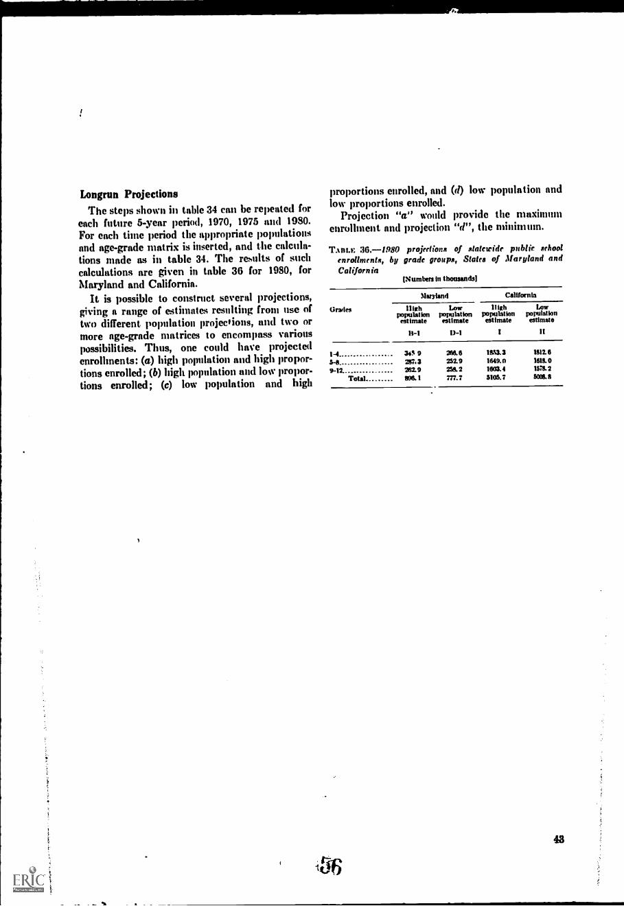
Longrun ProjectionsThe steps shown in table 34 can be repeated for
each future 5-year period, 1970, 1975 and 1980.For each time period the appropriate populationsand age-grade matrix is inserted, and the calcula-tions made as in table 34. The results of suchcalculations are given in table 36 for 1980, forMaryland and California.
It is possible to construct several projections,giving a range of estimates resulting from use of
two different population projections, and two ormore age-grade matrices to encompass variouspossibilities. Thus, one could have projectedenrollments: (a) high population and high propor-tions enrolled; (6) high population and low propor-tions enrolled; (c) low population and high
proportions enrolled, and (d) low population andlow proportions enrolled.
Projection "a" would provide the maximumenrollment and projection "d", the minimum.
TABLE 36.-1M projections of statewide public schoolenrollments, by grade groups, Stales of Maryland andCalifornia
(Numbers In thousands)
Grades
Maryland
Meipopulationestimate
11-1
Lowpopulationestimate
D-1
California
11 fahpopulationestimate
Lowpopulationestimate
It
1-43-89-12
Total.
34% 920.3262.9896. 1
266.6232.9WA 2777. 7
1833. 31649.01803.43105.7
1812.61618.01578.2BOOS. 8
48
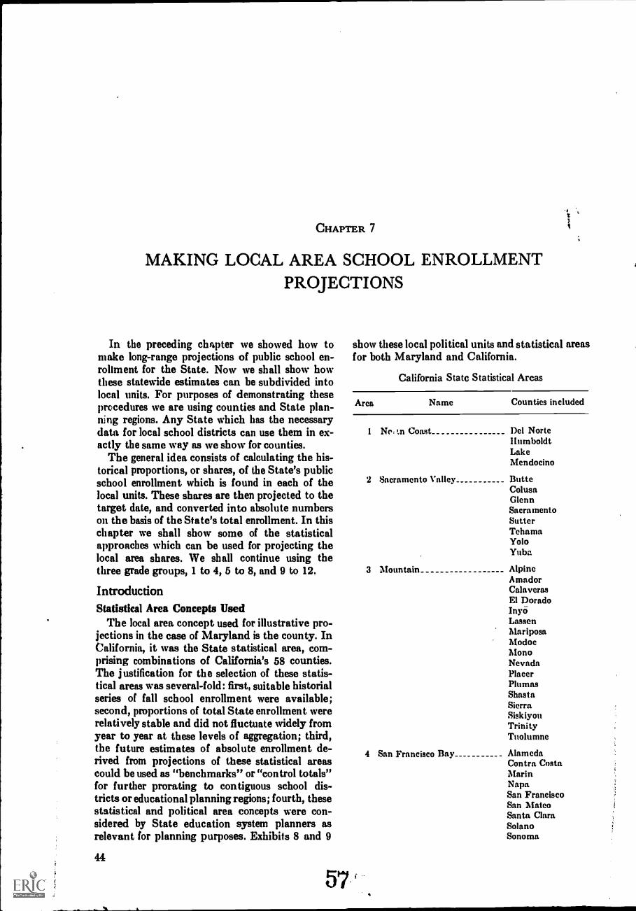
CHAPTER 7
MAKING LOCAL AREA SCHOOL ENROLLMENTPROJECTIONS
In the preceding chapter we showed how to show these local political units and statistical areasmake long-range projections of public school en- for both Maryland and California.roltment for the State. Now we shall show howthese statewide estimates can be subdivided into California State Statistical Areas
local units. For purposes of demonstrating theseprocedures we are using counties and State phtn- Area Name Counties included
ning regions. Any State which has the necessarydata for local school districts can use them in ex- I Ne.tn Coast Del Norte
actly the same way as we show for counties. HumboldtLake
The general idea consists of calculating the his- Mendocinotorical proportions, or shares, of the State's publicschool enrollment which is found in each of the 2 Sacramento Valley Butte
Colusalocal units. These shares are then projected to the Glenntarget date, and converted into absolute numberson the basis of the State's total enrollment. In this
SacramentoSutter
chapter we shall show some of the statistical Tchama
approaches which can be used for projecting the YoloYnblocal area shares. We shall continue using the
three grade groups, 1 to 4, 5 to 8, and 9 to 12. 3 Mountain AlpineAmador
Introduction CalaverasEl Dorado
Statistical Area Concepts Used InyäThe local area concept used for illustrative pro- Lassen
jections in the case of Matyland is the county. In MariposaModocCalifornia, it was the State statistical area, com- Mono
prising combinations of California's 58 counties. NevadaThe justification for the selection of these statis- Placertical areas was several-fold: first, suitable historial Plumas
series of fall school enrollment were available; ShastaSierrasecond, proportions of total State enrollment were Siskiyou
relatively stable and did not fluctuate widely from Trinityyear to year at these levels of aggregation; third, Tutolumnethe future estimates of absolute enrollment de-
4 San Francisco Bay Alamedarived from projections of these statistical areas Contra Costacould be used as "benchmarks" or "control totals" Marinfor further prorating to contiguous school dis- Napa
tricts or educational planning regions; fourth, these San Francisco
statistical and political area concepts were con- San MateoSanta Clara
sidered by State education system planners as Solanorelevant for planning purposes. Exhibits 8 and 9 Sonoma
44
57
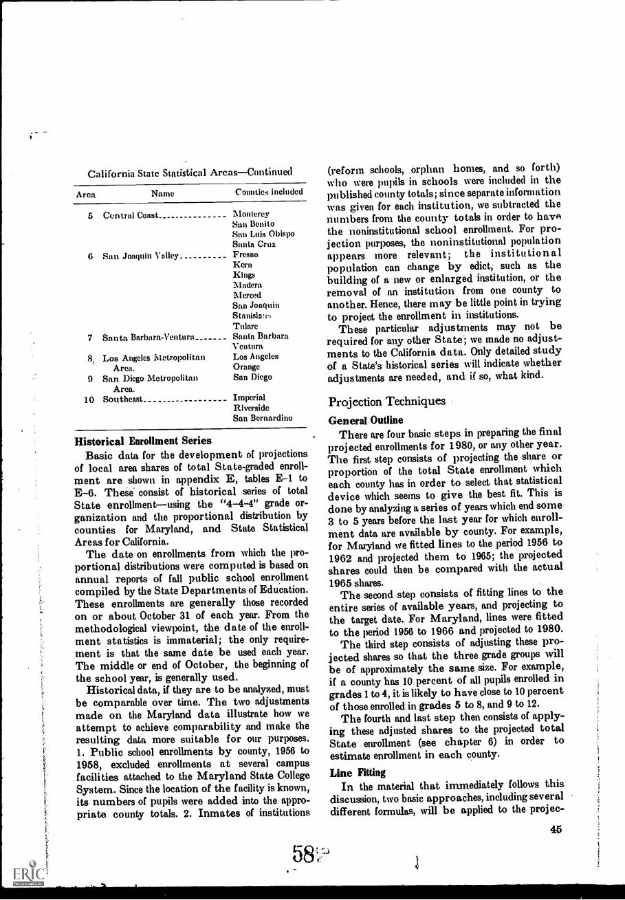
California State Statistical AreasContinued
Area Name Counties included
5 Central Coast MontereySan BenitoSan Luis ObispoSanta Cruz
6 San Joaquin Valley FresnoKernKingsA.laderaMercedSan JoaquinStanislivv,Tulare
7 Santa Barbara-Ventura Santa BarbaraVentura
8, Los Angeles MetropolitanArea.
Los AngelesOrange
9 San Diego Metropolitan San DiegoArca.
10 Southeast ImperialRiversideSan Bernardino
Historical Enrollment SeriesBasic data for the development of projections
of local area shares of total State-graded enroll-ment are shown in appendix E, tables E-1 toE-6. These consist of historical series of totalState enrollmentusing the "4-4-4" grade or-ganization and the proportional distribution bycounties for Maryland, and State StatisticalAreas for California.
The date on enrollments from which the pro-portional distributions were computed is based onannual reports of fall public school enrollmentcompiled by the State Departments of Education.These enrollments are generally those recordedon or about October 31 of each year. From themethodological viewpoint, the date of the enroll-ment statistics is immaterial; the only require-ment is that the same date be used each year.The middle or end of October, the beginning ofthe school year, is generally used.
Historical data, if they are to be analyzed, mustbe comparable over time. The two adjustmentsmade on the Maryland data illustrate how weattempt to achieve comparability and make theresulting data more suitable for our purposes.1. Public school enrollments by county, 1956 to1958, excluded enrollments at several campusfacilities attached to the Maryland State CollegeSystem. Since the location of the facility is known,its numbers of pupils were added into the appro-priate county totals. 2. Inmates of institutions
,"
(reform schools, orphan homes, and so forth)who were pupils in schools were included in thepublished county totals; since separate informationwas given for each institution, we subtracted thenumbers from the county totals in order to haw,the noninstitutional school enrollment. For pro-jection purposes, the noninstitutional populationappears more relevant; the institutionalpopulation can change by edict, such as thebuilding of a new or enlarged institution, or theremoval of an institution from one county toanother. Hence, there may be little point in tryingto project the enrollment in institutions.
These particular adjustments may not berequired for any other State; we made no adjust-ments to the California data. Only detailed studyof a State's historical series will indicate whetheradjustments are needed, and if so, what kind.
Projection Techniques
General OutlineThere are four basic steps in preparing the final
projected enrollments for 1980, or any other year.The first step consists of projecting the share orproportion of the total State enrollment whicheach county has in order to select that statisticaldevice which seems to give the best fit. This isdone by analyzing a series of years which end some3 to 5 years before the last year for which enroll-ment data are available by county. For example,for Maryland we fitted lines to the period 1956 to1962 and projected them to 1965; the projectedshares could then be compared with the actual1965 shares.
The second step consists of fitting lines to theentire series of available years, and projecting tothe target date. For Maryland, lines were fittedto the period 1956 to 1966 and projected to 1980.
The third step consists of adjusting these pro-jected shares so that the three grade groups willbe of approximately the same size. For example,if a county has 10 percent of all pupils enrolled ingrades 1 to 4, it is likely to have close to 10 percentof those enrolled in grades 5 to 8, and 9 to 12.
The fourth and last step then consists of apply-ing these adjusted shares to the projected totalState enrollment (see chapter 6) in order toestimate enrollment in each county.
Line FittingIn the material that immediately follows this
discussion, two basic approaches, including severaldifferent formulas, will be applied to the projec-
45
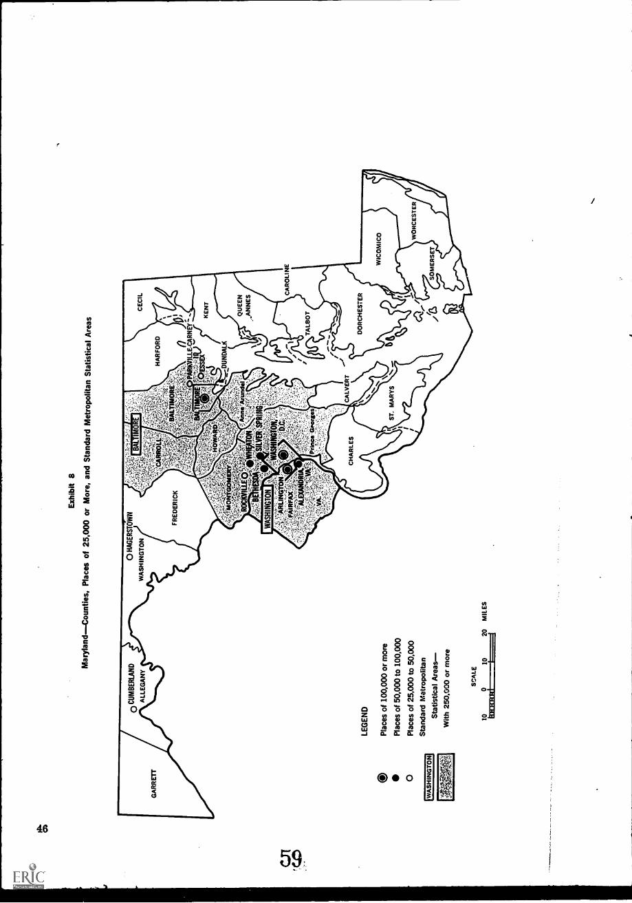
Exh
ibit
8
Mar
ylan
dCou
ntie
s, P
lace
s of
25,
000
or M
ore,
and
Sta
ndar
d M
etro
polit
anS
tatis
tical
Are
as
pii4
,4i:d
orse
s
WA
SH
ING
TO
N
ZW
,".+
1,:z
e;,.
LEG
EN
D
Pla
ces
of 1
00,0
00 o
r m
ore
Pla
ces
of 5
0,00
0 to
100
,000
Pla
ces
of 2
5,00
0 to
50,
000
Sta
ndar
d M
etro
polit
an
Sta
tistic
al A
reas
With
250
,000
or
mor
e
10
SC
ALE
010
20M
ILE
S
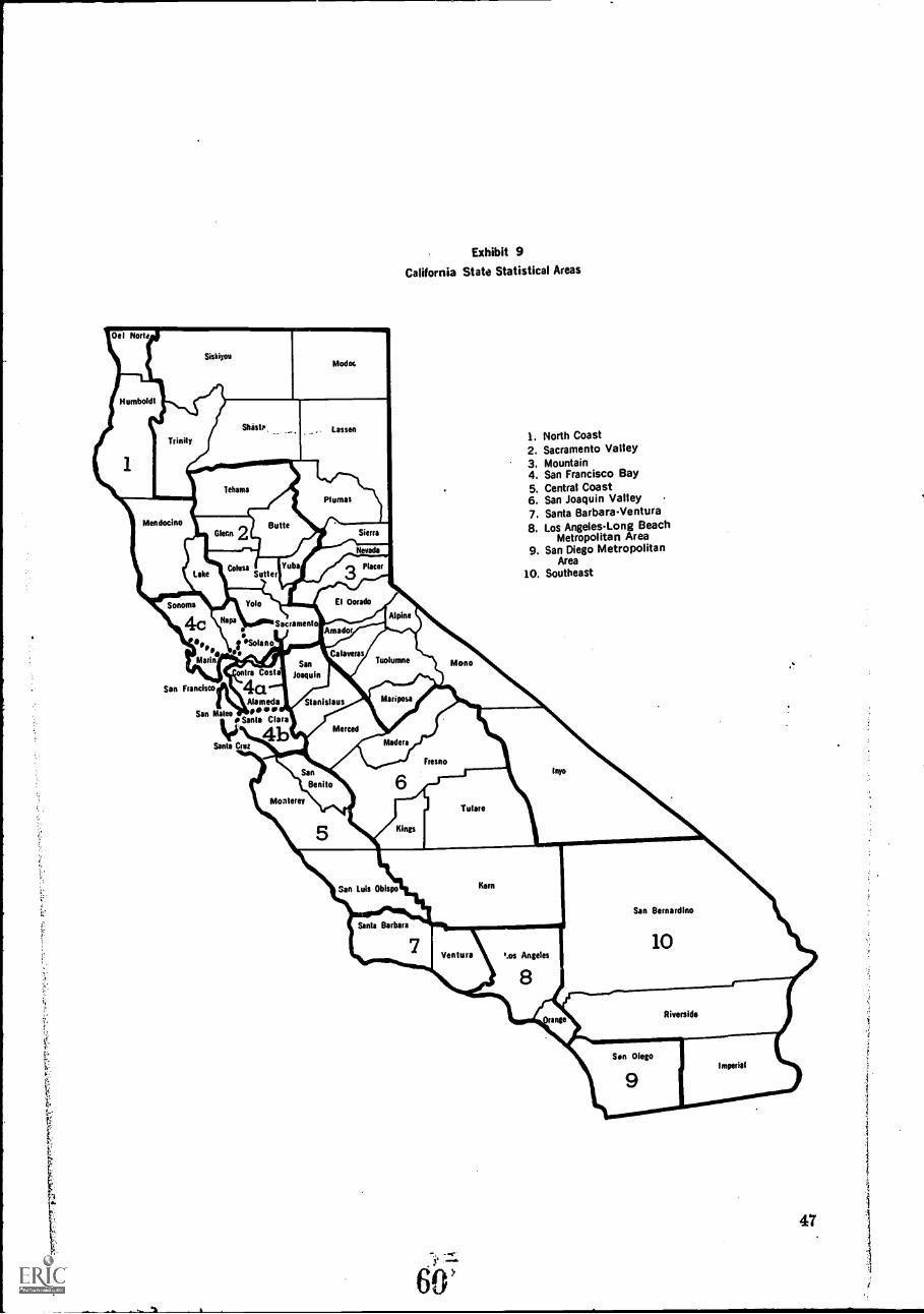
Exhibit 9California State Statistical Areas
1. North Coast2. Sacramento Valley3. Mountain4. San Francisco Bay5. Central Coast6. San Joaquin Valley7. Santa Barbara-Ventura8. Los AngelesLong Beach
Metropolitan Area9. San Diego Metropolitan
Area10. Southeast
San Francisco aAlameda
San MateoVSanta Clara
Santa Cruz
47
c
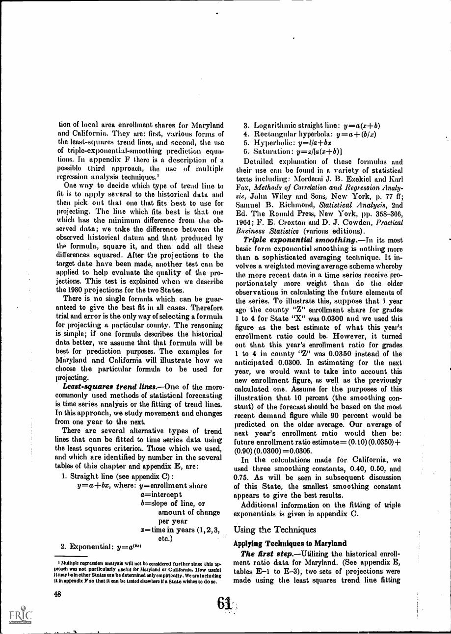
tion of local area enrollment shares for Marylandand California. They are: first, various forms ofthe least-squares trend lines, and second, the useof triple-exponen tial-smoo thing prediction equa-tions. In appendix F there is a description of apossible third approach, the use of multipleregression analysis techniques.'
One way to decide which type of trend line tofit is to apply several to the historical data andthen pick out that one that fits best to use forprojecting. The line which fits best is that onewhich has the minimum difference from the ob-served data; we take the difference between theobserved historical datum and that produced bythe formula, square it, and then add all thesedifferences squared. After the projections to thetarget date have been made, another test can beapplied to help evaluate the quality of the pro-jections. This test is explained when we describethe 1980 projections for the two States.
There is no single formula which can be guar-anteed to give the best fit in all cases. Thereforetrial and error is the only way of selecting a formulafor projecting a particular county. The reasoningis simple; if one formula describes the historicaldata better, we assume that that formula will bebest for prediction purposes. The examples forMaryland and California will illustrate how wechoose the particular formula to be used forprojecting.
Least-squares trend lines.One of the more.commonly used methods of statistical forecastingis time series analYsis or the fitting of trend lines.In this approach, we study movement and changesfrom one year to the next.
There are several alternative types of trendlines that can be fitted to time series data usingthe least squares criterion. Those which we used,and which are identified by number in the severaltables of this chapter and appendix E, are:
1. Straight line (see appendix C):y=a+bx, where: y=enrollment share
a= intercep tb=slope of line, or
amount of changeper year
x= time in years (1,2,3,etc.)
2. Exponential: y=a(bz)
I Multiple regression analysis will not be considered further since this ap-proach was not particularly useful for Maryland or California. Ifow usefulI t may be in ether States can be determined only empirically. We are includingit in appendix F so that it can be tested elsewhere if a State wishes to do so.
48
3. Logarithmic straight line: y=a(x+b)4. Rectangular hyperbola: y=a+(blx)5. Hyperbolic: y=11a-Fbx6. Saturation: y=xl[a(x+b)]Detailed explanation of these formuhts and
their use can be found in a variety of statisticaltexts including: Mordecai J. B. Ezekiel and KarlFox, Methods qf Correlation and Regression Analy-sis, John Wiley and Sons, New York, p. 77 ft ;Samuel B. Richmond, Statistical Analysis, 2ndEd. The Ronald Press, New York, pp. 358-366,1964; F. E. Croxton and D. J. Cowden, PracticalBusiness Statistics (various editions).
Triple exponential smoothing.In its mostbasic form exponential smoothing is nothing morethan a sophisticated averaging technique. it in-volves a weighted moving average scheme wherebythe more recent data in a time series receive pro-portionately more weight than do the olderobservations in calculating the future elements ofthe series. To illustrate this, suppose that 1 yearago the county "Z" enrollment share for grades1 to 4 for State "X" was 0.0300 and we used thisfigure as the best estimate of what this year'senrollment ratio could be. However, it turnedout that this year's enrollment ratio for grades1 to 4 in county "Z" was 0.0350 instead of theanticipated 0.0300. In estimating for the nextyear, we would want to take into account thisnew enrollment figure, as well as the previouslycalculated one. Assume for the purposes of thisillustration that 10 percent (the smoothing con-stant) of the forecast should be based on the mostrecent demand figure while 90 percent would bepredicted on the older average. Our average ofnext year's enrollment ratio would then be:future enrollment ratio estimate= (0.10) (0.0350) +(0.90)(0.0300)=0.0305.
In the calculations made for California, weused three smoothing constants, 0.40, 0.50, and0.75. As will be seen in subsequent discussionof this State, the smallest smoothing constantappears to give the best results.
Additional information on the fitting of tripleexponentials is given in appendix C.
Using the Techniques
Applying Techniques to MarylandThe first step.Utilizing the historical enroll-
ment ratio data for Maryland. (See appendix E,tables E-1 to E-3), two sets of projections weremade using the least squares trend line fitting
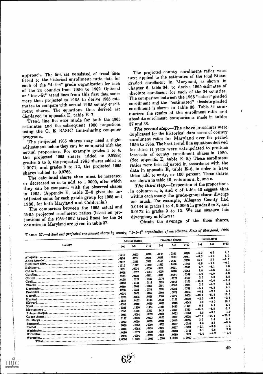
approach. The first set consisted of trend linesfitted to the historical enrollment ratio data foreach of the "4-4-4" grade organization for eachof the 24 counties from 1956 to 1962. Optionalor "best-fit" trend lines from this first data series
were then projected to 1965 to derive 1965 esti-
mates to compare with actual 1965 county enroll-ment shares. The equations thus derived aredisplayed in appendix E, table E-7.
Trend line fits were made for both the 1965estimates and the subsequent 1980 projectionsusing the G. E. BASIC time-sharing computerprograms.
The projected 1965 shares may need a slightadjustment before they can be compared with theactual proportions. For example grades 1 to 4,
the projected 1965 shares added to 0.9988;
grades 5 to 8, the projected 1965 shares added to1.0071, and grades 9 to 12, the projected 1965shares added to 0.9768.
The calculated shares then must be increasedor decreased so as to add to 1.0000, after which
they can be compared with the observed sharesin 1965. (Appendix E, table E-8 gives the un-adjusted sums for each grade group for 1965 and1980, for both Maryland and California.)
The comparison between the 1965 actual and1965 projected enrollment ratios (based on pro-jections of the 1956-1962 trend lines) for the 24counties in Maryland are given in table 37.
The projected county enrollment ratios werenext applied to the estimates of the total State-graded enrollment in Maryland, as shown inchapter 6, table 34, to derive 1965 estimates ofabsolute enrollment for each of the 24 counties.The comparison between the 1965 "actual" gradedenrollment and the "estimated" absolute-gradedenrollment is shown in table 38. Table 39 sum-marizes the results of the enrollment ratio andabsohite-enrollment comparisons made in tables37 and 38.
The second step.-The above procedures wereduplicated for the historical data series of countyenrollment ratios for Maryland over the period1956 to 1966. The hest trend line equations derivedfor these 11 years were extrapolated to prold9t8ice
forecasts of county enrollment shares in(See appendix E, table E-9.) These enrollmentratios were then adjusted in accordance with thedata in appendix E, table E-8, in order to havethem add to unity, or 100 percent. These sharesare shown in table 40, columns a, b, and c.
The third step.-Inspection of the proportionsin columns a, b, and c of table 40 suggest thatwithin each county the grade-group shares divergetoo much. For example, Allegany County had0.0144 in grades 1 to 4, 0.0065 in grades 5 to 8, and0.0172 in grades 9 to 12. We can measure thisdivergency as follows:
Obtain the average of the three shares,
TABLE 37.-Aclual and projected enrollment sheres by county, "4-4-4" organization, of enrollment, State of Maryland, 1986
CountyActual shares Projected shares Percent error
1-1 5-8 9-12 1-1 5-8 9-12 1-4 5-8 9-12
Allegany0210 . 0223 .0276 .0199 . 0237 .0283 -5. 2 0.3 2. 5
Anne Arundel0834 .0704 .0685 .0832 . 0760 . 0741 -0. 2 -4.3 8. 2
Baltimore City.2117 . 2241 . 2391 .2448 . 2437 . 2350 15. 6 8.7 -1. 7
Baltimore. 1510 . 1517 . 1650 .1522 . 1480 . 1648 0.8 -2.4 -O. 1
Calvert0078 . 0074 . 0056 .0084 . 0071 . 0057 7. 7 -4.1 1. 8
Caroline0068 . 0072 .0061 . 0070 . 0070 . 0063 2.9 -2.8 3. 3
Carroll. 0188 .0178 .0161 .0171 . 0164 . 0168 -9.0 -7.9 4. 3
Cecil.0165 .0127 .0132 .0170 . 0129 .0137 3.0 1. 6 3. 8
Charles.0150 .0151 .0118 .0133 . 0148 . 0109 -11.3 -2.0 -7. 6
Dorchester0089 . 0007 .0082 .0091 . 0092 . 0088 2. 2 -5.2 7. 3
Frederick0238 .0234 .0233 .0218 .0224 .0238 -8. 4 -4.3 2. 1
Garrott0074 0073 . 0062 .0069 . 0071 .0063 -6.8 -2. 7 1. 8
Hartord 0323 .0305 .0264 .0264 . 0270 . 0305 -12. 1 -11.5 15.5
Howard .0157 . 0152 .0143 . 0153 . 0151 .0139 -2.5 -0. 7 -2. 8
Kent 0052 .0049 . 0039 .0053 . 0048 . 0013 1.9 -2.0 10. 3
Montgomery. 1221 . 1360 . 1454 .1228 . 1443 . 1477 0.6 6. 1 1. 6
Prince Georges. 1600 1492 . 1399 .1419 . 1369 . 1312 -14.0 -8.2 6. 2
Queen Armes.,0061 . 0064 . 0052 .0005 .0062 . 0053 6.5 -3. 1 1. 9
St. Marys .0127 . 0100 .0123 .0105 .0091 .0008 -17.3 -14. 1 -20. 3
Somerset0062 .0069 . 0053 .0004 . 0070 .0058 3.2 1. 4 9. 4
Talbot 0066 .0062 .0059 . 0069 .0067 . 0054 4. 5 8. 1 -8. 5
Washington0296 .0288. .0295 .0280 . 0277 . 0299 -2. 1 -3.8 1. 3
Wicomico . 0186 .0179 .0139 . 0188 . 0180 . 0143 1. I 0.6 2. 9
Worcester.0088 .0001 . 0073 .0085 .0089 . 0074 -& 4 -2 2 -1. 4
Total 1.0000 1.0000 1. 0000 1.0000 1.0000 1.0000
49
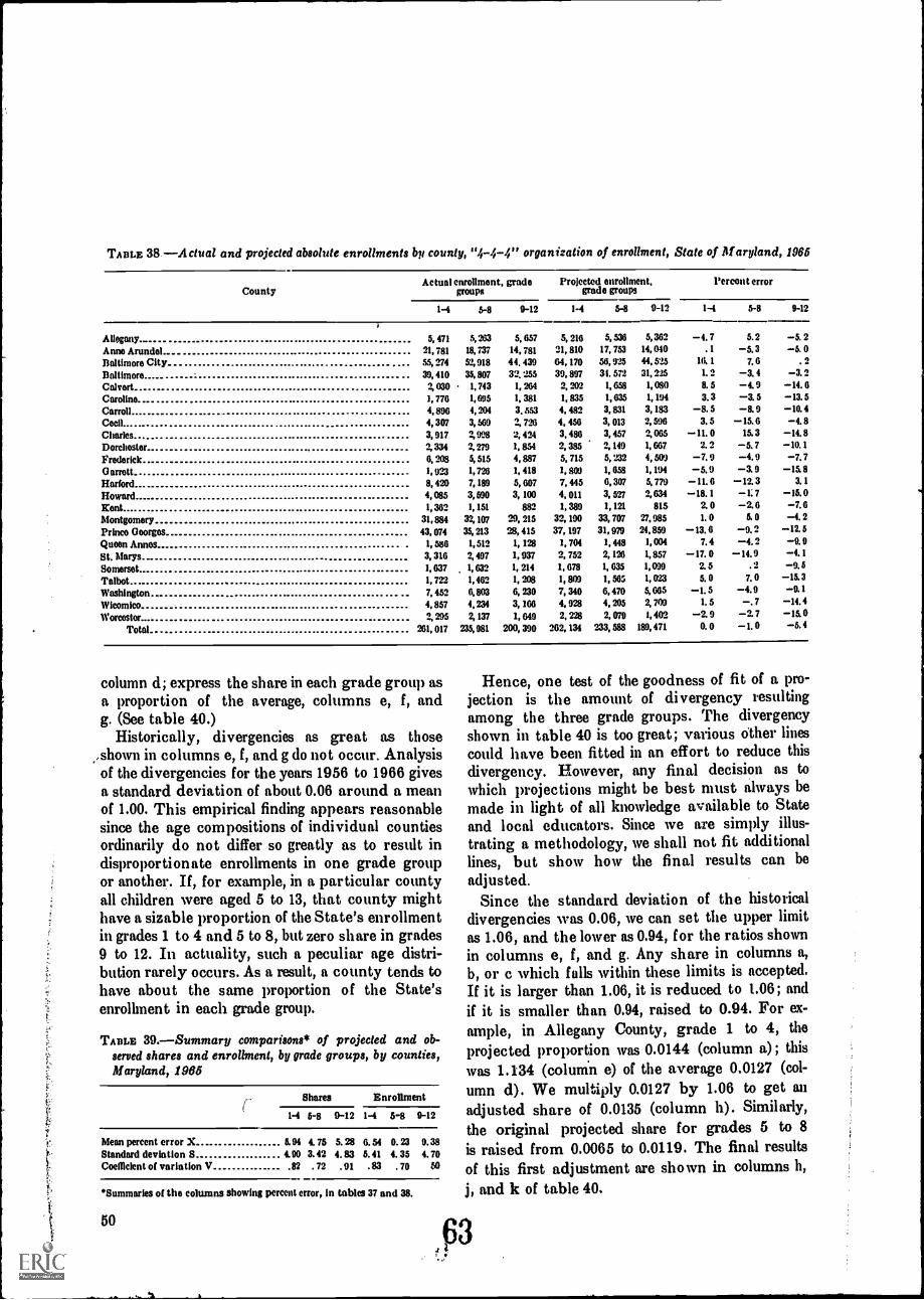
TABLE 38 Actual and projected absolute enrollments by county, "4-4-4" organization of enrollment, State of M aryland, 1965
CountyActual enrollment, grade
groupsProjected enrollment,
grade groupsPercent error
1-4 5-8 0-12 5-8 9-12 5-8 9-12
Allegany. 5, 471 5, 263 5, 657 5, 216 5, 536 5,362 4. 7 5. 2 5. 2Anne Arundel 21, 781 18, 737 14, 781 21, 810 17, 753 14, 040 . 1 5. 3 5. 0Balthnoro City SS, 274 52,918 44. 439 &I, 170 .56, 92.5 44, 52.5 I6. I 7. 6 . 2
Baltimore 39, 410 35, 807 32. 2.55 39, 897 31. 572 31, 225 1. 2 3. 4 3. 2Calvert 9, 030 1, 743 1, 264 2, 202 1, 658 1, 080 8. 5 4. 9 14. 6Caroline I, 776 1, 695 1, 381 1, 835 1, 635 1, 194 3. 3 3. 5 13. 5Carroll 4, 896 4, 204 3.553 4, 482 3, 831 3, 183 8. 5 8. 9 10.4Cecil 4, 307 3, 569 2, 720 4, 456 3, 013 2, 596 3. 5 I5. 6 4. 8Charles 3, 917 2,928 2, 424 3, 486 3, 457 2, 065 11. 0 15.3 14. 8Dorchester 9, 334 2, 279 1, 854 2, 385 2, 149 1, 667 2. 2 5. 7 10. 1Frederick 6, 208 5, 515 4, 887 5, 715 5, =2 4, 509 7.43 4. 9 7. 7Garrett 1,923 1,726 1, 418 1,803 1,658 1,194 5.9 3.9 15.8Harford 8, 420 7, 189 5, 607 7, 445 6, 307 5, 779 11. 6 12. 3 3. 1
Howard 4, 085 3, 690 3, 100 4, 011 3, 527 2, 634 18. 1 1: 7 16. 0Sent 1,362 I, 151 882 1, 389 1, 121 815 2. 0 2.6 7.6Montgomery 31, 884 3Z 107 29, 215 32, 190 33, 707 27, 985 1. 0 5. 0 4. 2Prince Georges 43, 074 35, 213 %, 415 37, 197 31, 979 24, 859 13. 6 9. 2 12. 5Queen Annos 1,536 1,512 1, 128 1,704 1,448 1,004 7.4 4. 2 9.0St. Marys 3, 316 2, 497 1, 937 2, 752 2, 126 1, 857 17. 0 14.9 4. 1Somerset i. 637 1, 632 1, 214 1, 678 1, 635 1,099 2. 5 . 2 9. 5Talbot 1, 722 1,462 1,208 1,809 1,565 1,023 5. 0 7. 0 15.3Washington 7, 452 6,803 6, 230 7, 340 6, 470 5, 665 1. 5 4.9 0.1Wicomico 4, 857 4, 234 3, 166 4, 928 4, 205 2, 709 1. 5 .7 14. 4
Worcester. 2, 295 2, 137 1, 649 2, 228 2, 070 1,402 2. 9 2. 7 15. 0
Total 261, 017 235,981 200, 390 262, 134 233, 588 189, 471 0. 0 1. 0 5. 4
column d; express the share in each grade group asa proportion of the average, columns e, f, andg. (See table 40.)
Historically, divergencies as great as those/shown in columns e, f, and g do not occur. Analysisof the divergencies for the years 1956 to 1966 givesa standard deviation of about 0.06 around a meanof 1.00. This empirical finding appears reasonablesince the age compositions of individual countiesordinarily do not differ so greatly as to result indisproportionate enrollments in one grade groupor another. If, for example, in a particular countyall children were aged 5 to 13, that county mighthave a sizable proportion of the State's enrollmentin grades 1 to 4 and 5 to 8, but zero share in grades9 to 12. In actuality, such a peculiar age distri-bution rarely occurs. As a result, a county tends tohave about the same proportion of the State'senrollment in each grade group.
TABLE 39.Summary comparisons* of projected and ob-served shares and enrollment, by grade groups, by counties,Maryland, 1965
Shares Enrollment
1-4 5-8 0-12 1-4 5-8 9-12
Mean percent error X & 94 4. 75 5. 28 6. 54 6. 23 9.38Standard deviation S . 4.90 3.42 4. 83 5. 41 4. 35 4. 70
Coefficient of variation .82 . 72 .91 .83 . 70 60
Summaries of the columns showing percent error, in tables 37 and 38.
50
Hence, one test of the goodness of fit of a pro-jection is the amount of divergency resultingamong the three grade groups. The divergencyshown in table 40 is too great ; various other linescould have been fitted in an effort to reduce thisdivergency. However, any final decision as towhich projections might be best must always bemade in light of all knowledge available to Stateand local educators. Since we are simply illus-trating a methodology, we shall not fit additionallines, but show how the final results can beadjusted.
Since the standard deviation of the historicaldivergencies was 0.06, we can set the upper limitas 1.06, and the lower as 0.94, for the ratios shownin columns e, f, and g. Any share in columns a,b, or c which falls within these limits is accepted.If it is larger than 1.06, it is reduced to 1.06; andif it is smaller than 0.94, raised to 0.94. For ex-ample, in Allegany County, grade 1 to 4, theprojected proportion was 0.0144 (column a); thiswas 1.134 (colunin e) of the average 0.0127 (col-
umn d). We multiply 0.0127 by 1.06 to get anadjusted share of 0.0135 (column h). Similarly,the original projected share for grades 5 to 8is raised from 0.0065 to 0.0119. The final resultsof this first adjustment are shown in columns h,j, and k of table 40.
63
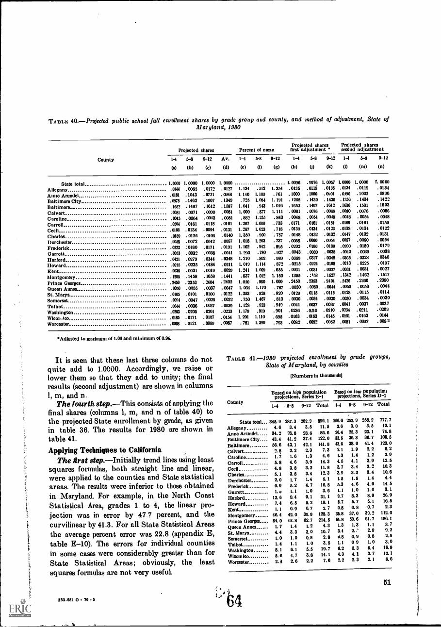
TABLE 40.-Projected public school fall enrollment shares by grade group and county, and method of adjustment, State ofMaryland, 1980
Projected shares Percent of meanProjected sharesfirst adjustment
Projected sharessecond adjustment
County 1-4
(a)
5-8
(b)
9-12
(c)
Av.
(d)
1-4
(e)
5-8
(f)
9-12
(g)
1-8
(11)
5-8
(i)
9-12
(k)
1-4
(I)
5-8
(m)
9-12
(n)
State total 1 0000 1.0000 1.0000 1.0000 1.0090 .9076 1. 0057 I. 0000 1. 0000 f. 0000
Allegany .0144 .0065 .0172 . 0127 I. 134 .512 1. 354 . 0135 . 0119 . 0135 . 0134 . 0119 . 0134
Anne Arundel . 0181 . 1043 .0721 . 0948 I. 140 1.100 . 701 . 1000 . 1000 . 0001 .0)90 . 1002 . 0896
Baltimore City .0978 . 1462 . 1607 . 1349 . 725 1. 084 1. 191 . 1208 . 1430 . 1430 . 1250 . 1434 . 1422
Baltimore.. 1650 1497 . 1012 . 1587 1. 041 .943 I. 016 . 1652 .1497 . 1612 . 1636 . 1501 . 1003
Calvert 0081 . 0071 . 0090 . 0081 1. OM .877 I. III . 0081 . 0070 . 0086 . 0080 . 0076 . 0080
Caroline. 0064 . 0043 . 0051 .882 1.255 . 843 .0048 . 0054 . 0048 .0018 . 0054 . 0048
Carroll .0204 .0161 . 0118 . 0161 1.267 1.000 . 733 . 0171 . 0161 . 0151 .0109 . 0101 . 0150
Cecil .0100 . 0134 .0004 . 0131 1. 207 1. 023 . 718 . 0139 . 0134 . 0123 .0133 . 0131 . 0122
Charles .0189 . 0120 . 0100 . 0140 1.350 .900 . 757 . 0148 . 0112 . 0132 .0147 . 0132 . 0131
1)orchestor .0058 . 0072 . 0042 . 0057 1. 018 1. 263 . 737 . 0058 . 0000 . 0054 .0057 . 0060 . 0054
Frederick .0222 :0180 .0171 . 0191 1. 162 .942 . 895 . 0202 .0180 . 0180 .0200 . 0180 . 0179
Garrett 0053 . 0032 .0038 . 0041 1. 293 .780 .927 . 0043 . 0039 . 0038 .0943 . 0039 . 0038
Harford. .0121 . 0279 . 0344 . 0348 1.210 .802 . 989 . 0369 .0327 . 0348 . 0365 . 03% . 0346
Howard .0215 .0235 . 0184 . 0211 1. 019 1.114 . 872 . 0215 . 0224 . 0198 . 0213 . ons . 0197
Kent .0036 . 0031 . 0019 . 0029 I. 241 1. 069 . 055 . 0031 . C031 . 0027 . 0031 . 0031 . 0027
Montgomery .1206 . 1458 . 1058 . 1441 .837 1. 012 1.150 . 1355 . 458 . 1527 .1342 . 1462 . 1517
Prince Georges .2450 . 2353 . 2404 . 2402 1. 020 .980 1. 003 . 2450 . 2353 . 2401 .2420 . Z360 . 2390
Queen Amos_ 0050 . 0055 . 0037 . 0047 I. 064 1.170 . 787 . 0050 . 0050 . 0044 .0050 . 0050 . 0044
St. Marys. .0105 . 0101 .0100 . 0122 1. 353 .828 .820 . 0129 .0115 . 0115 .01% . 0115 . 0114
Somerset 03024 . 0047 . 0026 . 0332 . 750 1.467 . 813 . 0030 . 0034 . 0030 .0030 . 0034 . 0030
Talbot 0044 . 0036 . 0037 . 0039 1. 128 . 923 . 949 . 0041 . 0037 . 0037 . 0041 . 0037 0037
Washington .0263 . 0205 .0201 . 0223 1.179 .919 . 901 . 0M6 .0210 . 0210 .0%4 . 0211 . 0209
Wicot leo. .0185 . 0171 . 0107 0154 1.201 1.110 . 095 . 0163 . 0163 . 0145 .0101 . 0163 . 0144
Worcester .0068 . 0121 . 0069 . 0087 . 781 1.390 . 793 . 0082 . 0092 . 0082 . 0081 . 0092 008 2
'Adjusted to maximum of 1.00 and minimum of 0.94.
It is seen that these last three columns do notquite add to 1.0000. Accordingly, we raise orlower them so that they add to unity; the finalresults (second adjustment) are shown in columns1, m, and n.
The fourth step.-This consists of applying thefinal shares (columns 1, m, and n of table 40) tothe projected State enrollment by grade, as givenin table 36. The results for 1980 are shown intable 41.
Applying Techniques to CaliforniaThe first step.-Initially trend lines using least
squares formulas, both straight line and linear,were applied to the counties and State statisticalareas. The results were inferior to those obtainedin Maryland. For example, in the North CoastStatistical Area, grades 1 to 4, the linear pro-jection was in error by 47 7 percent, and thecurvilinear by 41.3. For all State Statistical Areasthe average percent error was 22.8 (appendix E,table E-10). The errors for individual countiesin some cases were considerably greater than forState Statistical Areas; obviously, the leastsquares formulas are not very useful.
353-581 0 - 70.5
TABLE 41.-1980 projected enrollment by gradeState of Maryland, by counties
(Numbers in thousands)
groups,
County
Based on high population Based on /ow populationprojections, Series 11-1 projections, Series 1)-1
1-4 5-8 0-'32 Total 1-4 5-8 9-12 Total
State total... 345. 9 287. 3
Allegany. ..... 4. 6 3. 4
Anne Arundel__ 34. 2Baltimore City.... 43. 4
Baltimore......... 56. 6
Calvert 2
Caroline ..... 1. 7
Carroll 5. 8Cecil 4. 8
Clmrles 5. 1
Dorchcster 2. 0
Frederick 6. 9
Garrett 1.0Harford 12.
Howard 7. 4
Kent I. 1
Montgomery 46. 4
Prince Georges 84. 0Queen Annes 1. 7
St. Marys 4. 4
Somerset 1.0Talbot 1. 4
Washington 8. 1
Wicom leo 5. 6Worcester 2.3
%. 841. 243. 1
2. 21.04.63. 83. 81. 75.21. 1
9. 46. 50. 9
42. 067. 81.43. 31. 01.16. 1
4. 72. 6
202.93.5
23.37.492. 1
2. 31.33.93.23.41.44. 71.09.15. 2O. 7
39.962. 7
1. 2
3.00.81. 05. 53. 82. 2
890. 111. 5
86. 6122. 0141. 8
7. 34. 6
14. 311. 812. 35. 1
16. 83.
31. 119. 12. 7
128. 3214. 5
4. 310. 7
2. 83. 5
19. 714. I7.6
266.61 6
26.433.543.6
2.11.34.53.73.91.55.31.1
9.75.70.8
35.864.81.33.46.81.16.24.32.2
252. 9 258. 23. 0 3. 5
25. 3
36. 338. 0
1.91. 4
4. 13. 43. 31. 54. 6I. 08. 35. 7O. 8
37. 059. 6
I. 3
0.90 95. 34. 12. 3
23. I36. 741. 4
2. 21. 23. 93. 23. 4I. 44. 6I. 08.95. 1O. 7
39. 261. 7
1. 1
2. 9O. 8
1. 05. 43. 72. 1
777. 710. I74. 8
100. 5123. 0
6. 23.9
12. 510. 310. 64. 4
14. 53. I26.916. 52. 3
112. 0186. 1
3. 79. 22. 53. 0
16. 912. 1
6.0
51
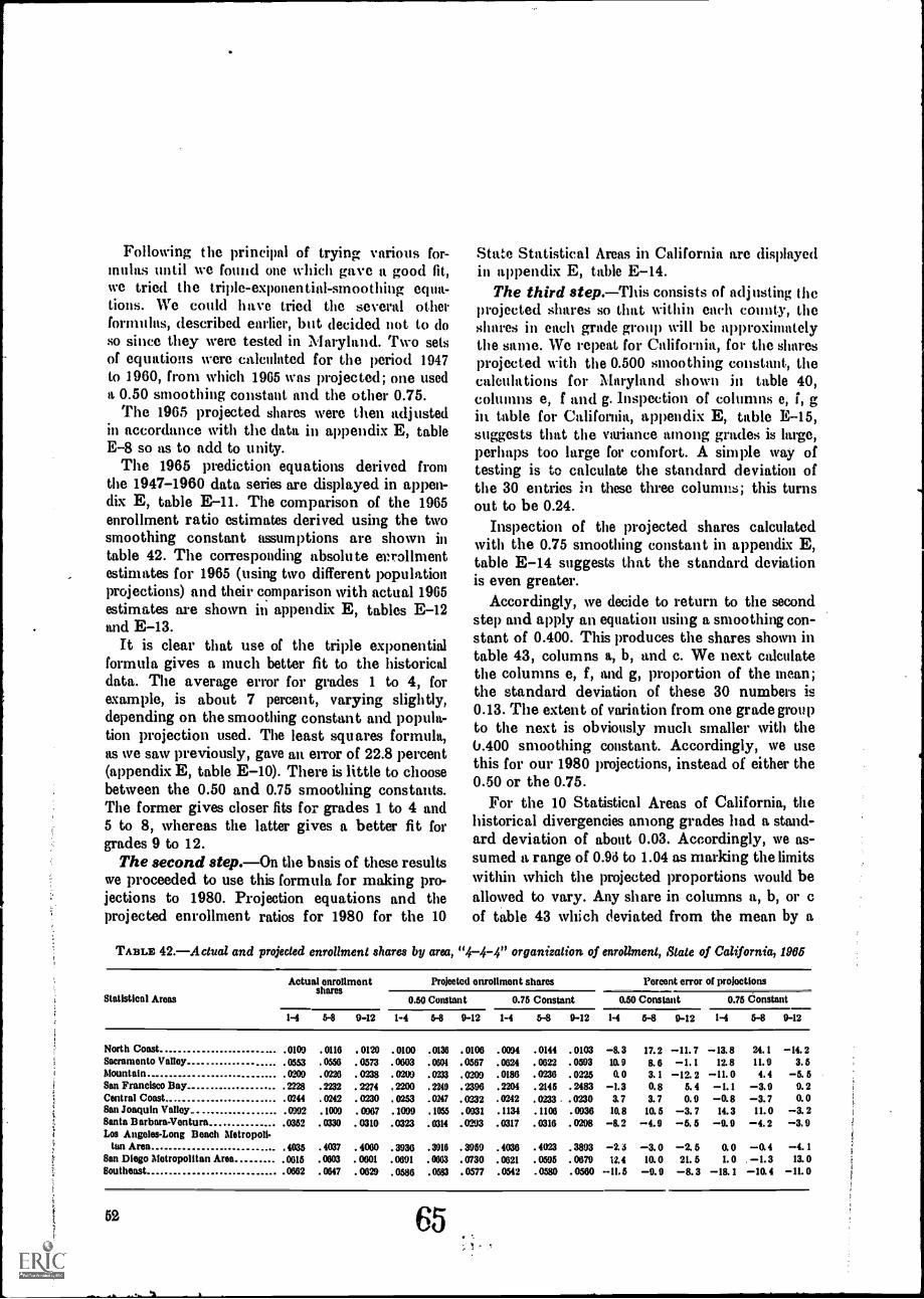
Following the principal of trying various for-mulas until we found one which gave a good tit,we tried the triple-exponential-smoothing equa-tions. We could have tried the several otherformulas, described earlier, but decided not to doso since they were tested in Maryland. Two setsof equations were calculated for the period 1947to 1960, from which 1965 was projected; one useda 0.50 smoothing constant and the other 0.75.
The 1965 projected shares were then adjustedin accordance with the data in appendix E, tableE-8 so as to add to unity.
The 1965 prediction equations derived fromthe 1947-1960 data series are displayed in appen-dix E, table E-11. The comparison of the 1965enrollment ratio estimates derived using the twosmoothing constant assumptions are shown intable 42. The corresponding absolute ei:rollmentestimates for 1965 (using two different populationprojections) and their comparison with actual 1965estimates are shown in appendix E, tables E-12and E-13.
It is clear that use of the triple exponentialformula gives a much better fit to the historicaldata. The average error for grades 1 to 4, forexample, is about 7 percent, varying slightly,depending on the smoothing constant and popula-tion projection used. The least squares formula,as we saw previously, gave an error of 22.8 percent(appendix E, table E-10). There is little to choosebetween the 0.50 and 0.75 smoothing constants.The former gives closer fits for grades 1 to 4 and5 to 8, whereas the latter gives a better fit forgrades 9 to 12.
The second step.-On the basis of these resultswe proceeded to use this formula for making pro-jections to 1980. Projection equations and theprojected enrollment ratios for 1980 for the 10
State Statistical Areas in California are displayedin appendix E, table E-14.
The third step.-This consists of adjusting theprojected shares so that within each county, theshares in each grade group will be approximatelythe same. We repeat for California, for the sharesprojected with the 0.500 smoothing constant, thecalculations for Maryland shown in table 40,columns e, f and g. Inspection of columns e, 1, gin table for California, appendix E, table E-1 5,suggests that the variance among grades is large,perhaps too large for comfort. A simple way oftesting is to calculate the standard deviation ofthe 30 entries in these three columns; this turnsout to be 0.24.
Inspection of the projected shares calculatedwith the 0.75 smoothing constant in appendix E,table E-14 suggests that the standard deviationis even greater.
Accordingly, we decide to return to the secondstep and apply an equation using a smoothing con-stant of 0.400. This produces the shares shown intable 43, columns a, b, and c. We next calculatethe columns e, f, and g, proportion of the mean;the standard deviation of these 30 numbers is0.13. The extent of variation from one grade groupto the next is obviously much smaller with the0.400 smoothing constant. Accordingly, we usethis for our 1980 projections, instead of either the0.50 or the 0.75.
For the 10 Statistical Areas of California, thehistorical divergencies among grades had a stand-ard deviation of about 0.03. Accordingly, we as-sumed a range of 0.96 to 1.04 as marking the limitswithin which the projected proportions would beallowed to vary. Any share in columns a, b, or cof table 43 which deviated from the mean by a
TABLE 42.-Aclual and projected enrollment shares by area, "4-4-4" organization of enrollment, State of California, 1966
Statistical Areas
Actual enrollmentshares
Projected enrollment shares Percent error of projections
0.50 Constant 0.75 Constant 0.50 Constant 0.75 Constant
1-4 5-8 9-12 1-4 5-8 9-12 1-4 5-8 9-12 1-4 5-8 9-12 1-4 5-8 9-12
North Coast 0109 . 0116 . 0120 . 0100 . 0136 . 0106 . 0094 . 0144 . 0103 -8. 3 17. 2 -11. 7 -13. 8 24. I -14. 2Sacramento Valley 0553 . 0556 . 0573 . 0603 . 0004 . 0567 . 0624 . 0622 . 0593 10. 9 8. 6 -1. 1 12. 8 11. 9 3. 5Mountain 0009 0226 . 0238 . 0209 . 0233 . 0209 . 0186 . . 0225 0. 0 3. I -12. 2 -II. 0 4. 4 -5. 5San Francisco Bay 2228 . 2232 . 2274 . 2200 . 2249 . 2396 . 2204 . 2145 . 2483 -I. 3 0. 8 5. 4 -1. 1 -3. 9 9. 2Central Coast 0244 . 0242 . . 0253 . 0247 . . 0242 . 0233 . 0230 3. 7 3. 7 0. 9 -0.8 -3. 7 0. 0San Joaquin Valley. 099* . 1009 . 0967 . 1099 . 1055 . 0931 . 1134 . 1106 . 0936 10.8 10. 5 -3. 7 14. 3 11. 0 -3. 2Santa Barbara-Ventura 0352 . 0330 . 0310 . 0323 . 0314 . 0293 . 0317 . 0316 . 0298 -8. 2 -4. 9 -5. 5 -9. 9 -4. 2 -3. 9Los Angeles-Long Beach Metropoli-
tan Area 4035 . 4037 . 4060 . 3936 .3916 . 3959 . 4036 . 4023 . 3893 -2. -3. 0 -2. 5 0. 0 -O. 4 -4. 1San Diego Metropolitan Area 0615 . 0603 . 0601 . 0691 . 0063 . 0730 . 0621 . 0595 . 0679 12.4 10. 0 21. 5 1. 0 -1. 3 13. 0Southeast 0662 . 0647 . 0629 . 0586 . 0583 . 0577 . 0542 . 0580 . 0560 -II. 5 -9. 9 -8. 3 -18. 1 -10.4 - II. 0
52
.._
65
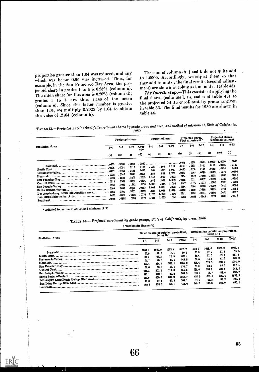
proportion greater than 1.04 was reduced, and anywhich was below 0.96 was increased. Thus, forexample, in the San Francisco Bay Area, the pro-jected share in grades 1 to 4 is 0.2324 (column a).The mean share for this area is 0.2023 (column d) ;
grades 1 to 4 are thus 1.148 of the mean(column e). Since this latter number is greaterthan 1.04, we multiply 0.2023 by 1.04 to obtainthe value of .2104 (column h).
The sum of columns h, j and k do not quite addto 1.0000. Accordinqly, we adjust them so thatthey add to unity; the final results (second adjust-ment) are shown in columns!, In, an(1 n (table 43).
The fourth step.-Th is consists of a pplying thefinal shares (columns 1, in, and n of table 43) tothe projected State enrollment by grade as givenin table 36. The final results for 1980 are shown intable 44.
TABLE 43.-Projected public school fall enrollment shares by grade group and area, and method of adjustment, State of California,
.1980
Statistical Areas
Projected shares Percent of mean Projected shares, Projected slmres,First tuljustment Second adjustment
1-4
(a)
5-8
(b)
9-12
(c)
Aver-age
(d)
1-4
(e)
5-8 9-12
(g)
1-4
(h)
5-8
(j)
9-12
(k)
1-1
(I)
5-8
(m)
9-12
(n)
State total . 9609 . 9503 . 9569 . 9560 .9574 .9569 .9638 1.0000 1.0000 1.0000
North Coast .0108 . 0691 . 0117 . 0105 1. 028 866 1. 114 . 0108 . 0101 . 0109 . 0113 . 0106 . 0113
Sacramento Valley . 0432 . 0383 . 0424 . 0413 I. 046 . 927 1. 026 .0430 . 0396 . 0424 . 0449 . 0414 . 0440
Mountain . . 0247 . 0348 0278 . 856 . 888 1. 251 . 0267 . 0267 . . 0279 . 0279 . 0300
San F rancisco Bay2324 . 1938 . 1806 . 2023 1. 148 . 957 . 892 .2104 . 1942 . 1942 . 2198 . 2030 . 2015
Central Coast . 0315 . 0304 . 0353 . 0324 . 972 . 938 1089 . 0315 . 0311 . 0337 . 0329 . 0325 . 0350
San Joaquin Valley . 1247 . 1083 . 1342 . 1224 1.018 .884 1.096 .1247 . 1175 .1273 .1302 .1228 .1321
Santa Barbara-Ventura . 0599 . 0597 . 0191 . 0562 L 005 1. 062 . 873 . 0584 . 0584 . 0540 . 0610 . 0610 . 05.60
Los Angeles-Long Beach Metropolitan Area 3086 . 3599 . 3752 . 3479 . 887 1. 034 1. 078 . 3340 . 3599 . 3618 . 3489 . 3761 . 3753
San Diego Metropolitan Aroa . 0472 . 0459 . 0198 0376 I. 255 1. 220 . 526 . 0391 . 0391 . 0361 . 0408 . 0409 . 0375
Southeast . 0788 . 0802 . 0738 . 0776 1. 015 1. 033 . 051 . 0788 . 0802 . 0745 . 08U . 0838 . 0773
Adjusted to maximum of 1.04 and minimum of .06.
TABLE 44.-Projected enrollment by grade groups, State of California, by areas, 1980
(Numbers in thousands)
Statistical Areas
Based on high population projections,Series B-1
Based on low population projections,Series D-1
1-4 5-8 0-12 Total 1-4 1-8 9-12 Total
State total1853. 3 1640. 0 1603. 4 5105. 7 1812. 6 1618. 0 1578. 2 5008. 8
North Coast20, 9 17. 5 18. 1 56. 5 70. 5 17. 2 17. 8 55. 5
Sacramento Valley83. 2 68. 3 70. 5 222. 0 81. 4 67. 0 69. 4 217. 8
Mountain51. 7 46. 0 48. 1 145. 8 50. 6 48. 1 47. 3 143. 0
San Francisco Bay407. 4 334. 7 323. 1 1008. 2 398. 4 - 328. 5 318. 0 1044. 9
Central Coast61. 0 53. 6 56. 1 170. 7 59. 6 52. 6 55. 2 167. 4
San Joaquin Valley241. 3 202. 5 211. 8 655. 6 236. 0 198. 7 208. 5 643. 2
Santa Barbara-Ventura.113. 1 100. 6 89. 8 303. 5 110. 6 98. 7 88. 4 297. 7
Los Angeles-Long Beach Metropolitan Aro&646. 6 620. 2 601. 9 1868. 7 632. 3 608. 4 592. 4 1833. 1
San Diego Metropolitan Aron75.6 67. 4 60. 1 203. 1 74.0 66.2 59. 2 199. 4
Southeast152. 5 138. 2 123. 0 414. 6 149. 2 135. 6 122. 0 406. 8
53
CHAPTER 8
PROJECTING A SINGLE SCHOOL DISTRICT
The previous chapters were concerned withprocedures which could be utilized by a centralState agency for preparing projections for each ofits counties and school _districts. Our reasons torpreferring a statewide approach were set forthin chapter 2, where we discussed the difficulties ofstudying individual school districts, especiallythose which are very small or whose geographicboundaries have been changed in recent years, orexpect boundary changes within the foreseeablefuture. It is recognized, nevertheless, that inmany instances no estimates prepared by a centralState agency will be available to the local schooldistrict, and the local unit will wish to have 3omeestimate of its possible elementary and high schoolenrollment for a decade or longer. Accordingly,in this chapter we are presenting some procedureswhich are modified versions of those previouslydescribed, and which can be used by any schooldistrict. Short-term projections, 1 to 5 years inthe future, were described in chapters 3 and 4 andneed no further elaboration here.
Types of School Districts
Before describing any pmjection techniques,it is best to review the several types of schooldistricts, because each type requires its own kindof projection methods. The first major distinctionis between those districts which have maintainedconstant geographic boundaries over a number ofyears, and expect to keep those boundaries intact,at least, until the projection date; and thosedistricts which have had, or expect to have,significant boundary changes.
Within each of these two types are those schooldistricts which provide education from kinder-garten through high school; and those whichprovide a certain number of years schooling afterwhich the students are sent to another district.Perhaps the most common form is that in which
54
the local district, provides the elementary school-ing and a consolidated district provides the highschool. Thus, for the purposes of projectingenrollment, two or more school districts areinvolved.
Within each of these latter two types, thedistricts can be subdivided further into at leastthree size groups: very small, enrollment under1,000 students per year; intermediate, from 1,000to 100,000; very large districts such as New YorkCity, Chicago, or any similar metropolis.
Further complications to plague the statisticianare sometimes introduced when the geographicboundaries are changed and simultaneously, thedistrict moves from a kindergarten through highschool program to One covering only part of theentire elementary and high school education.Such districts can only be handled on an ad hocbasis and will not be described here.
Some school districts have boundary lines whichdo not coincide with any political or censusboundaries. Such places have additional dacultiesin obtaining the basic population data needed formaking projections; we shall offer some suggestionson how to cope with this problem.
Finally, there are some districts which arenonoperating. The making of enrollment projec-tions for such places may be simple for the non-operating unit, but poses some problems for thedistrict which does the actual teaching. We shallsuggest ways of handling this type of situation.In summary, because of the large variety of schooldistrict types, we shall discuss a variety of ap-proaches. Officials of a school district can thenselect the procedure, or combination of procedures,most appropriate to their particular needs.
Basic Projection Techniques
Two variants of what we call the Basic Projec-tion Teclmique, and the circumstances under
which each is applicable, win be described.Three conditions are necessary for t he applicationof both of these variants, and these are:
1. They apply to school districts having be-tween 1,000 and 100,000 pupils. School officialsfrom snmller or larger districts can use them also
if they so desire; however, these veiy small andvery large districts often have unique situationswhich do not lend themselves readily to theapplication of a standard technique. Indeed,even a district 1 1WAXA falls -h0.iWeell the aboverange, and to which the Basic Projection Tech-nique presumably can be applied, shoukl considerwhether or not it has unique situations or prob-lems which would preclude the use of a standardtechnique. For example, if the officials of a schooldistrict containing 1,200 pupils know that severallarge entermises are slated to move into the areaand can be expected to double its populationwithin, say, the next 5 years, then they musttake this into account in projecting school enroll-ment. The application of a standard techniquecannot take such an unusual event into account.
2. The school district must have had constantand unchanging boundaries for a significantlylong period, and the expectation is that theboundaries will continue unchanged until, atleast, the pmjection date. The first variant ofour Basic Projection Technique uses DecennialCensus data; this requires that the boundarieshave remained unchanged for at least three Cen-sus periods and will continue unchanged. In theillustrations used here, we shall employ datafrom the 1940, 1950 and 1960 population censusesand shall project to 1980; hence we must haveconstant boundaries over the 40 year period,1940 to 1980. When the 1970 Census results be-come available, data for 1950, 1960, and 1970can be used for projecting to 1980. In the eventthat the district's boundaries have changed, amodification in the procedures is required andwill be discussed in a section entitled "ChangingBoundaries."
The second variant of the Basic ProjectionTechnique uses locally available school enrollmentdata. For this, data should be available for atleast 10 years, and preferably more, for a districthaving unchanging boundaries. In the illustrationgiven, historical data are presented for the period1955 to 1968, 14 years, and then projected to1980.
3. For the first variant, we also must have dis-tricts whose boundary lines conform to recognized
political lines such as a county or city, or conformto the boundaries of one or more minor civildivisions as published in the Decennial Popula-tion Censuses of the United States. For suchschool districts it is possible to obtain the necessarydata from the published Census voluoes. Thetreatment of those districts which do not haverecognized political boundary lines are discussed
in the section on nonconforming boundary linas.
For the second variant it is possible to useschool districts whose boundaries do not conform
to recopuzed political lines. Nevertheless, it isdesirable that. such districts lie within one county,although projections can be madealbeit withmore workif they cross county lines.
Finally, we should note that it is desirable fora school district to make projections using bothvariants, if possible. They should be compared,scrutinized carefully, and evaluated in terms of
land use information and other facts known tothe local community and which cannot be takeninto account via general statistical procedures.On the basis of such an examination, a decisioncan be made as to which projection to accept, orhow to modify them in light of additional locallyavailable information.
Variant OneProcedures covering grades 1 through 12
This can be used in school districts whose bound-aries conform to recognized political boundaries.The general idea consists of relating the populationof school age in the local school district, to thesame ago population in the county for three Censusperiods, using published decennial data. Thepopulation of school age in the county is thenrelated to the same population in the State. Pro-jections to 1980 follow immediately since we havepopulation projections for all States, prepared bythe U.S. Census Bureau. We can then work fromthese State figures to the local school district.The sequence of steps (shown in table 45) is asfollows:
1. We wish to use data from the most recentthree Decennial Population Censuses; for presentpurposes we shall use data for 1940, 1950, and 1960.
2. Copy out the humbers of persons aged 5 to17 years living in the State at each date. For 1940the data will be found in Vol. II, in the appro-priate State section; 1950 data appear in the PBseries, and 1960 statistics in the PC (1) B serics.
3. Next copy out the numbers of persons aged
55
6t3e,t
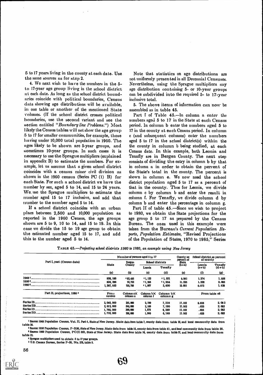
5 to 17 years living in the county at each date. Usethe same sources as for step 2.
4. We next wish to have the numbers in the 5-to 17-year age group living in the school districtat each date. As long as the school district bound-aries coincide with political boundaries, Census(Into showing age distributions will be available,in one table or another of the mentioned Statevolumes. (If the school district crosses politicalboundaries, use the second variant and see thesection entitled "Boundary line Problems.") Mostlikely the Census tables will not show the age group5 to 17 for smaller conmiunities, for example, thosehaving under 10,000 total population in 1960. Theages likely to be shown are 5-year groups, andsometimes 10-year groups. In such cases it isnecessary to use the Sprague multipliers (explainedin appendix B) to estimate the numbers. For ex-ample, let us assume that a given school districtcoincides with a census minor civil division asshown in the 1960 census (Series PC (1) B) foreach State. For such a school district we have thenumber by sex, aged 5 to 14, and 15 to 24 years.We. use the Sprague multipliers to estimate thenumber aged 15 to 17 inclusive, and add thatnumber to the number aged 5 to 14.
If a school district coincides with an urbanplace between 2,500 and 10,000 population asreported in the 1960 Census, the age groupsshown are 5 to 9, 10 to 14, and 15 to 19. In thiscase we divide the 15 to 19 age group to obtainthe estimated number aged 15 to 17, and addthis to the number aged 5 to 14.
Note that statistics on age distributions aronot uniformly presented in all Decennial Censuses.Nevertheless, using the Sprague multipliers anyage distribution containing 5- or 10-year groupscan be subdivided into the required 5- to 17-yearinclusive total.
5. The above items of information can now beassembled as in table 45.
Part T of Table 45.In column a enter thenumbers aged 5 to 17 in the State at each Censusperiod. In column b enter the numbers aged 5 to17 in the county at each Census period. In columna (and subsequent columns) enter the numbersaged 5 to 17 in the school district(s) within thethe county in column b being studied, at eachCensus date. In this example, both Leonia andTenafly are in Bergen County. The next stepconsists of dividing the entry in column b by thatin column a in order to obtain the percent ofthe State's total in the county. The percent isshown in column e. We now need the schooldistrict population aged 5 to 17 as a percent ofthat in the county. Thus for Leonia, we dividecolumn c by column b and enter the result incolumn f. For Tenafly, we divide column d bycolumn b and enter the percentage in column g.
Part II of table 45.Since we wish to projectto 1980, we obtain the State projections for theage group 5 to 17 as prepared by the CensusBureau. The ones used in this example weretaken from the Bureau's Current Population Re-ports, Population Estimates, "Revised Projectionsof the Population of States, 1970 to 1985," Series
TABLE 45.Projecting school districts 1980 to 1980, an example using New Jersey
Number of persons aged 5 to 17 County aspercent of
School district as percentof county
Part I, past (Census data)State
(n)
BergenCounty
(b)
School districts Slate(b+a)
(e)
Leonia Tonally(c+ b) (db)
(0 (g)
Leonia
(c)
Tenafly
(d)
19901 838, 186 4 82,485 4 1, 133 4 1, 531 0. 841 I. 374 1. 8501950 2 834, 286 93,733 i I, 245 4 1,954 11.235 I. 328 2. 08519601 1,367, 953 135,785 4 1, 507 3, 000 13. 581 0. 073 1. 038
Part II, projections, 1980 1 From Column aX Column bX Column bX From table 46census column e column ( column g
Serlos III 2, 045, 000 351,000 2,190 7, 310 17.162 0.625 2. 08 3Series 1111 2, 012, 000 345,000 2, 160 7, 190 17.162 .625 2. 083Serlos ID 1, 796, 000 300,000 1,875 6, 250 17.162 .625 2. 083Series IID. 1, 719, 000 295,000 1, 840 6, 190 17.162 .625 2. 083
I Source: 1040 Population Census, Vol. II, Part 4, State of Now Jersey. State data from table 7, county data from table 22, and local community data fromtable 30.
2 Source: 1950 Population Census, P-B30, Slate of Now Jersey. State data from table 15, county data from tablo 91. and local community data from tablo 38.$ Source: 1960 Population Census, PC(I) 3211, State of Now Jersey. State data (rom table 16, county data from table 27, and local community datafrom
table 22.4 Sprague multipliers used to obtain 5 to 17 year groups./ U.S. Census Bureau, Series P-25, No. 375, table 5.
56
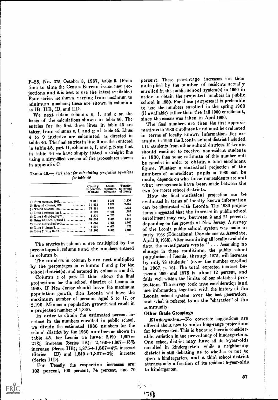
P-25, No. 375, October 3, 1967, table 5. (Fromtime to time the Census Bureau issues new pro-jections and it is best to use the latest available.)Four series are shown, varying from maximum tominimum numbers; these are shown in column a
as IB, IIB, ID, and IID.We next obtain columns e, f, and g on the
basis of the calculations shown in table 46. Theentries for the first three lines in table 46 aretaken from columns e, f, and g of table 45. Lines4 to 9 inclusive are calculated as directed intable 46. The final entries in line 9 are then enteredin table 4 5, part II, columns e, f, and g. Note thatin table 46 we have simply fitted a straight lineusing a simplified version of the procedures shown
in appendix C.
TABLE 46.Work sheet for calculating projection equationsfor table 45
County Leonia Tenaflyns percent ns percent as percento( State of county o( county
I) First census, 1940 9.841 1.374 I .&56
2) Second census, 1950 11 .235 1.328 2.086
3) Third census, 1960 13.581 0.973 1.938
4) Line 3 minus line I 3.740 .401 .082
5) Line 4 divided by 2 1 .870 .200 .041
6) Sum of lines 1, 2 and 3 34.657 3.675 5.879
7) Line 6 divided by 3 11 .552 1.225 1.960
8) Line 5 times 3 5.610 .600 .123
9) Line 7 plus line 8 17 .162 0.625 2.093
The entries in column a are multiplied by thepercentages in column e and the numbers enteredin column b.
The numbers in column b are next multipliedby the percentages in columns f and g for theschool district(s), and entered in columns c and d.
Column c of part II then shows the finalprojections for the school district of Leonia in
1980. If New Jersey should have the maximumpopulation growth, then Leonia will have themaximum number of persons aged 5 to 17, or2,190. Minimum population growth will result ina projected number of 1,840.
In order to obtain the estimated percent in-
crease in the numbers enrolled in public school,we divide the estimated 1980 numbers for theschool distriet by the 1960 numbers as shown intable 45. For Leonia we have: 2,190+1,807=21% increase (Series IB); 2,160-i-1,807=13%increase (Series IIB); 1,875-4-1,807=4% increase
(Series ID) and 1,840-i-1,807=2% increase
(Series IID).For Tenafly the respective increases are:
103 percent, 100 percent, 74 percent, and 70
percent. These percentage increases are thenmultiplied by the number of residents actuallyenrolled in the public school system(s) in 1960 inorder to obtain the projected numbers in publicschool in 1980. For these purposes it is preferableto use the mnnbers enrolled in the spring 1960(if available) rather than the fall 1960 enrollment,since the census was taken in April 1960.
The final numbers are then the first approxi-mations to 1980 enrollment and must be evaluatedin terms of locally known information. For ex-ample, in 1960 the Leonia school district included111 students from other school district.s. If Leoniashould continue to receive nonresident studentsin 1980, then some estimate of this number willbe needed in order to obtain a total enrollmentfigure. Whether a statistical projection of themnnbers of nonresident pupils in 1980 can bemade, depends on who these nonresidents are andwhat arrangements have been made between thetwo (or more) school districts.
How the final statistical projection con beevaluated in terms of locally known informationcan be illustrated with Leonia. The 1980 projec-tions suggested that the increase in public schoolenrollment may vary between 2 and 21 percent,depending on the growth of New Jersey. A surveyof the Leonia public school system was made inearly 1968 (Educational Developments Associate,
April 8, 1968). After examining all locally availabledata the investigators wrote " . . . Assuming nochange in these conditions, the public schoolpopulation of Leonia, through 1975, will increaseby only 78 students" (over the number enrolledin 1967, p. 16). The total expected increase be-tween 1960 and 1975 is about 12 percent, andfalls well within the limits of our statistical pro-jections. The survey took into consideratiop landuse information, together with the history of theLeonia school system over the last generation,and whal is referred to as the "character" of thecommunity.Other Grade Groupings
Kindergarten.No concrete suggestions areoffered about how to make long-range projectionsfor kindergarten. This is because there is consider-able variation in the prevalency of kindergartens.One school district may have all its 5-year-oldsenrolled in kindergarten while a neighboringdistrict is still debating as to whether or not toopen a kindergarten, and a third school districtattracts only a fraction of its resident 5-year-oldsto kindergarten.
'FA)
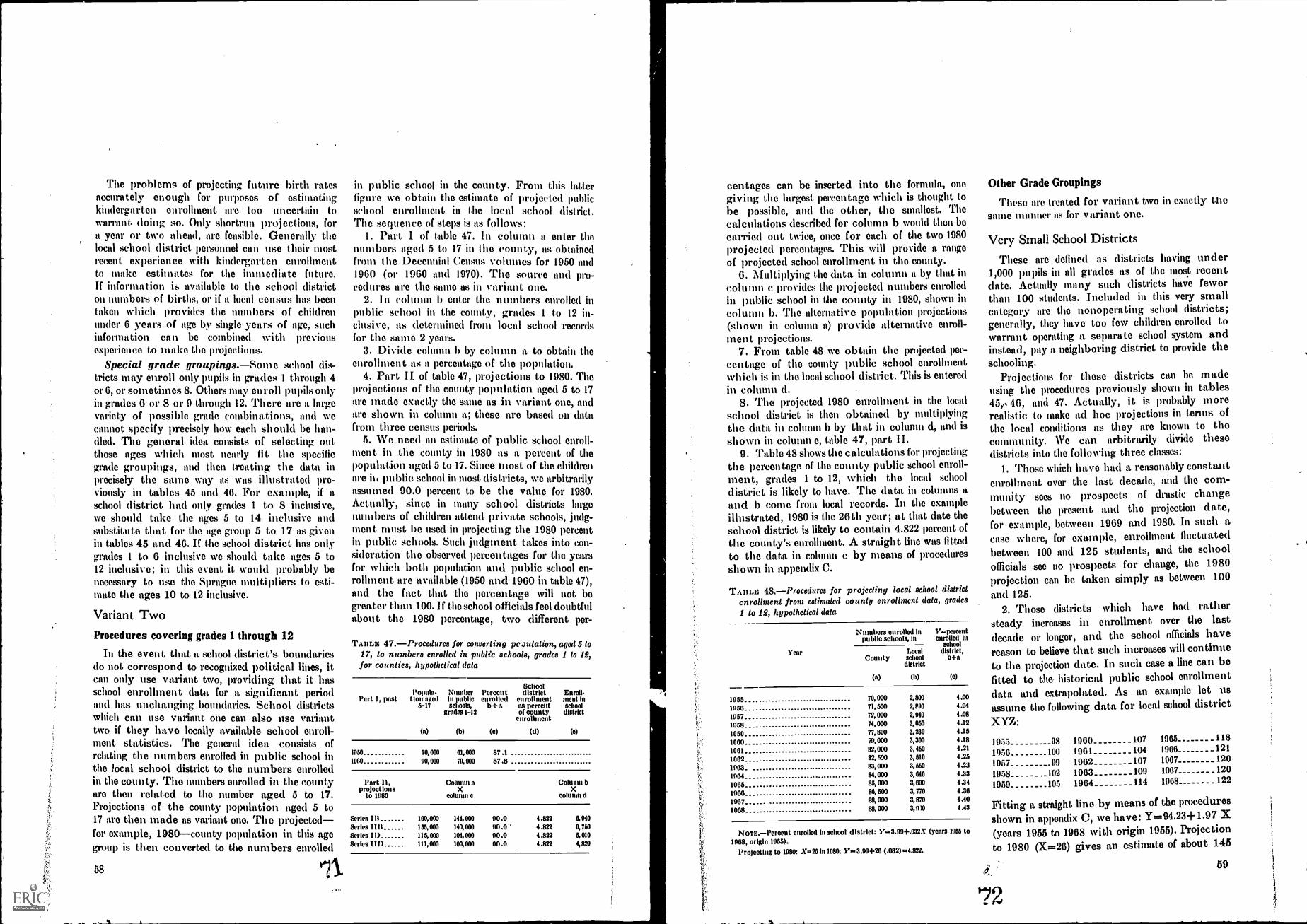
The problems of projecting future birth ratesaccurately enough for purposes of estimatingkindergarten enrollment are too uncertain towarrant. doing so. Only shortrun projections, fora year or two ahead, are feasible. Generally thelocal school district peNonnel can use their mostrecent experience with kindergarten enrollmentto make estimates for the hmnediate future.If information is available to the school districton numbers of births, or if a local census has beentaken which provides the numbers of chiklrenunder 6 years of age by single years of age, such'information can be combined with previousexperience to make the projections.
Special grade groupings.Some school dis-tricts nifty enroll only pupils in grades 1 through 4or 6, or sometimes 8. Others may enroll pupils onlyin grades 6 or 8 or 9 through 12. There are a largevariety of possible grade combinations, and wecannot specify precisely how each should be han-dled. The general idea consists of selecting outthose ages which most nearly fit the specificgrade groupings, aml then treating the data inprecisely the same way as was illustrated pre-viously in tables 45 and 46. For example, if aschool district, had only grades 1 to 8 inclusive,we should take the ages 5 to 14 inclusive andsubstitute that for the age group 5 to 17 as givenin tables 45 mmd 46. If the school district has onlygrades 1 to 6 inclusive we should take ages 5 to12 inclusive; in this event it would probably benecessary to use the Sprague multipliers to esti-mate the ages 10 to 12 inclusive.
Variant Two
Procedures covering grades 1 through 12
In the event that a school district's boundariesdo not correspond to recognized political lines, itcan only use variant two, providing that it hasschool enrollment data for a significant periodand has unchanging boundaries. School districtswhich can use variant one can also use varianttwo if they have locally available school enroll-ment statistics. The general idea consists ofrelating the numbers enrolled in public school inthe focal school district to the numbers enrolledin the county. The nmnbers enrolled in the countyare then related to the number aged 5 to 17.Projections of the county population aged 5 to17 are then made as variant one. The projectedfor example, 1980county population in this agogroup is then converted to the numbers enrolled
58 it
in public school in the county. From this latterfigure we obtain the estimate of projected publicschool enrollment in the local school district.The sequence of steps is as follows:
I. Part I of table 47. In column a enter themmibers aged 5 to 17 in the county, as obtainedfrifin the Decennial Census volumes for 1950 and1960 (or 1960 and 1970). The source and pro-cedures are the same as in variant one.
2. In column b enter the numbers enrolled inpublic school in the county, grades 1 to 12 in-clusive, as determined from local school recordsfor the same 2 years.
3. Divide cohnnn b by column a to obtain theenrollment, as a percentage of the population.
4. Part II of table 47, projections to 1980. Theprojections of the county population aged 5 to 17are made exactly the same as in variant one, andare shown in column a; these are based on datafrom three census periods.
5. We need an estimate of public school enroll-ment in the county in 1980 as a percent of thepopulation aged 5 to 17. Since most of the childrenare ii public school in most districts, we arbitrarilyassumed 90.0 percent to be the value for 1980.Actually, since in many school districts largenumbers of children attend private schools, judg-ment must be used in projecting the 1980 percentin public schools. Such judgment takes into con-sideration the observed percentages for the yearsfor which both population and public school en-rollment are available (1950 and 1960 in table 47),and the fact that the percentage will not begreater than 100. If the school officials feel doubtfulabout the 1980 percentage, two different per-
TAHLE 47.Procedures for converting pc isulation, aged 6 to17, to numbers enrolled in public schools, grades 1 to 12,for counties, hypothetical data
Part I, pastPoinila-
tion aged6-17
NumberIn publicsclmols,
grades 1-12
l'ercentenrolled
b +a
Schooldistrict
enrollmentas percentof county
enrollment
Enroll-ment inscimoldistrict
(a) (b) (e) (d) (0)
1950 70,000 01,000 87 .11000 90,000 79,000 87 .8
Part 11,projections
to 1980
ColunmX
column c
Column bX
column d
Series 1 11.Series 1111Series II)Series HI)
100,000
156, 000
114000111,000
144,000 90.0140, 000 90.0104,000 90.0100,000 00.0
4.8224.8224.8224.822
0,040
0,760
5,010
4,820
centages can be inserted into the formula, onegiving the largest percentage which is thought tobe possible, and the other, the smallest. Thecalculations described for column b would then becarried out twice, once for each of the two 1980projected percentages. This will provide a rangeof projected school enrollment in the county.
6. Multiplying the data in column a by that incolumn c provides the projected numbers enrolledin public school in the county in 1980, shown incolumn b. The alternative population projections(shown in column a) provide alternative enroll-ment projections.
7. From table 48 we obtain the projected per-centage of the county public school enrollmentwhich is in the local school district. 'rhis is enteredin column d.
8. The projected 1980 enrollment in the localschool district is then obtained by multiplyingthe data in column b by that in column d, and isshown in column e, table 47, part II.
9. Table 48 shows the calculations for projectingthe percentage of the county public school enroll-ment, grades 1 to 12, which the local schooldistrict is likely to have. The data in columns aand b conic from local records. In the exampleillustrated, 1980 is the 26th year; at that date theschool district. is likely to contain 4.822 percent ofthe county's enrollment. A straight line was fittedto the data in column c by means of proceduresshown in appendix C.
TABLE 48.Procedures for projecting local school districtenrollment from estimated county enrollment data, grades1 to 12, hypothetical data
Year
Numbers enrolled in V=percentpublic schools, in enrolled in
schoolLocal district,
County school b+adistrict
(b) (c)
1955 70,000 2,800 4.00
1956 71,500 2,P110 4.04
1057 72,000 2,940 4.08
1058 - . 74,000 3,050 4.12
1060 77, 800 3,230 4.15
1060 79,000 3,300 4 .18
1061 82, 000 3,450 4.21
1062 82, 500 3, 510 4.25
1963 83, 000 3, 550 4.23
1964 84, 000 3,640 4.33
1065 85, 000 3,690 4.34
1966 86, 500 3,770 4.36
1967 88, 000 3,870 4.40
1008 88, 000 3, 910 4.43
NOTE.Percent enrolled in school district: Y=3.09+.032X (years 1955 to1968, origin 1955).
Projecting to 1080: X=26 hi 1080; Y=3.09+26 (.032)=4.822.
Other Grade Groupings
These are treated for variant two in exactly thesame manner as for variant one.
Very Small School Districts
These are defined as districts having under1,000 pupils in all grades as of the most recentdate. Actually many such districts have fewerthan 100 students. Included in this very smallcategory are the nonoperating school districts;generally, they have too few children enrolled towarrant operating a separate school system andinstead, pay a neighboring district to provide theschooling.
Projections for these districts can be madeusing the pmcedures previously shown in tables45, 46, and 47. Actually, it is probably morerealistic to make ad hoc projections in terms ofthe local conditions as they are known to thecommunity. We can arbitrarily divide thesedistricts into the following three classes:
I. Those which have had a reasonably constantenrollment over the last decade, and the com-munity sees no prospects of drastic changebetween the present and the projection date,for example, between 1969 and 1980. In such acase where, for example, enrollment fluctuatedbetween 100 and 125 students, and the schoolofficials see no prospects for change, the 1980projection can be taken simply as between 100
and 125.2. Those districts which have had rather
steady increases in enrollment over the lastdecade or longer, and the school officials have
reason to believe that such increases will continue
to the projection date. In such case a line can befitted to the historical public school enrollmentdata and extrapolated. As an example let us
the following data for local school district
1955 98 1960 107 1905 _118
1956 100 1961 104 1900 . 121
1957 99 1962 107 1907 120
1958 102 1963 109 1907 120
1959 105 1964 114 1908 122
Fitting a straight line by means of the procedures
shown in appendix C, we have: Y=94.23+1.97 X(years 1955 to 1968 with origin 1955). Projection
to 1980 (X=26) gives an estimate of about 145
59
pupils to be enrolled at that date. The communityand school officials can now examine this statisticand evaluate it in terms of all other informationavailable about the possible future growth of thecommunity.
3. Those districts which have had rather consist-ent decreases in enrollment, and are likely to havefurther decreases. In this case exactly the sameprocedures suggested in step 2, are applied to ar-rive at an estimate for 1980. In this case the valuefor b will be negative.
Some districts may have mixed experiences andmust be treated on ait individual basis. Forexample, a district may have had a constant en-rollment of between 175 and 200 students everyyear for the last 20 years; it is known, however,that a new factory will be built and the popula-tion can be expected to increase by about 50 per-cent over the next decade. In such an event, a pro-jection to 1980 can be made by arbitrarily in-creasing enrollment by 50 percent, or to between250 and 300 pupils.
In the final analysis, projecting the enrollmentin very small school districts (including non-operating districts) involves judgment. There is nomechanical or statistical procedure which willautomatically provide the "correct" projectednumber. All statistical projections must beevaluated judgmentally in light of all other in-formation available.
Very Large School Districts
These are defined as districts having 100,000or more pupils; there are only between 20 and25 such districts in the United States. It is possibleto apply the basic projection technique as pre-viously described to such districts. Whether ornot this will be satisfactory in any particularschool district can be determined only by makingthe projection and then evaluating it in terms ofall other known factors. Since only a few momentsare required to make the calculations, it is ad-visable to do so, whether or not the results finallyare accepted or rejected.
As a general rule, the larger the school district,the more reason there is for treating it in the sameway as a State. The procedures described inchapters 6 and 7 for making State projections canbe applied to large cities. The basic problems con-sist of: obtaining a distribution of single years ofage by grade enrolled and by color (if du.; char-
60
acteristic is desired); obtaining tho 1980 (or otherfuture date) age distribution. These two problemscan be handled as follows:
Data showing the distribution by age and gradecan be obtained from the Census Bureau's Decen-nial Census data. If the desired tabulation is notpublished, perhaps a special tabulation can bepurchased. If this should turn out to be notfeasible, the school district can tabulate its owndata to show the numbers by single years of age bysingle grades, and by color, if desired. This shouldbe made for a Census year. From the publishedCensus statistics the numbers by color in eachsingle year of age in the total population can beobtained. If the data are shown only in 5-year agegroups, Sprague multipliers can be used to obtainsingle years of age. Using the numbers in the totalpopulation and the numbers enrolled in each grade,the age-grade matrix can be calculated, and thenprojected in exactly the same manner as for aState.
The second problem, that of obtaining a futurepopulation projection, is more complicated. Whenmaking State enrollment projections, we reliedon the State population projections made by theCensus Bureau and regularly published. As of1968, the Census Bureau has not publishedpopulation projections for large cities, but isfamiliar with the procedures for doing so. Ac-cordingly, we recommend that a school districtofficial interested in obtaining projections for hisdistrict, discuss this question with Census Bureaupersonnel. A variety of ways are available formaking the calculations, and the Census Bureaustatisticans can advise him as to the best pro-cedures to apply to his particular city.
In some States, a central State office preparespopulation projections for cities and sometimescounties. If this is not done, then the local schooldistrict personnel would have to prepare theprojections. Whether it has the trained personneland equipment needed to make such projectionsusing the same general procedures as those usedby the Census Bureau, can be determined only bythe individual local school board. The interestedreader will find descriptions of the Census Bureau'smethods in its publication P-25, No. 375 includedin appendix A, and in Population Estimates,"Projections of the Population of the UnitedStates by Age, Sex, and Color to 1990, withExtensions of Population by Age and Sex to 2015,"Series P-25, No. 381, December 19, 1967; pp.
1-50; and in Population Estimates, "Summary ofDemographic Projections," Serie,- P-25, No. 388,
March 14, 1968, pp 22-32, also included inappendix A.
Boundary Line ProblemsChanging Boundary Lines
The first requirement in making projections isthat the boundary lines for the projection date,for example, 1980, are known. If boundary linesare subject to unpredictable changes, and thelocal school district officials have no assuranceregarding future boundaries, then there is nopoint in making a projection. If it is believed thatpresent (i.e., at the time of making the projection)boundaries will be unchanged at the projectiondate, and it is known that during the last several
years there have been one br more significantboundary changes, then the school district has aproblem which is generally solvable.
Most school districts have boundaries whichcorrespond to political boundaries. For suchareas it is possible to obtain data on population byage from the Decennial Census volumes. Therefore,knowing the present boundaries of the district,it is often possible to reconstruct the populationat previous Census periods for the identicalpresent boundaries. This only involves locatingthe various geographic areas which comprisethe present district, and adding the Census data.Once having obtained the numbers aged 5 to 17at three successive Census dates, it is then possibleto apply variant one of the Basic ProjectionTechnique; if the district is very small, themodified version, as described under "Very smallschool districts," can be used. If local schoolenrollment data aro also available, then varianttwo also can be used.
Nonconforming Boundary Lines
If the public school enrollment data are avail-able, then variant two of the Basic ProjectionTechnique can be applied. If this information isnot available, then statistical projections aredifficult to make. Under these latter circumstances,the local school district officials must have knowl-edge regarding the munber of children living intheir area. They will know the current numberenrolled in the public schools by age and grade;indeed, this information may be available for ashort number of years prior, as well as the present.
The officials may not know how many youngsterswho live within their school district area attendprivate schools; nor are they likely to have anystatistical basis for making projections using theformula shown in tables 47 and 48 (or any otherstatistical projection formula).
Two devices that can help the school officialsin making judgments about possible futureenrollment aro the taking of a local populationcensus, and the making of a land use survey (seealso chapter 4). The former describes the demo-graphic situation as of the time of the census, andby containing informatiou on the numbers ofpreschool children by age, permits some estimatesof public school enrollment ed be made for the5 years following the date of the local census.
A land use survey fundamentally consists of aseries of judgments as to what may happen in thecommunity within the next several years, 10 or20 or more years, or whatever period the land usesurvey is designed to cover. Employing informa-tion on the amount of land available for com-mercial or industrial vs. residential use, togetherwith guesses as to how rapidly people may moveinto (or out of) the community, judgments aremade as to the possible number of school agechildren at some future date. Combining thisinformation with the data obtained from the localcensus which shows the division between publicand private school enrollments, some guesses canbe made as to future public school enrollment.
Projections by ColorWhether such projections can be made depend
in large measure on the availability of populationand public school enrollment by color. Censusprojections of State population by age are avail-able by color for the States having large numbersof nonwhites; Current Population Reports, Popu-lation Estimates, "Revised Projections of thePopulation of States, 1970 to 1985," (Series P-25,No. 375, October 3, 1967) contains projectionsof the nonwhites by age only for States having250,000 or more nonwhites in 1960. Data areavailable by color for the larger cities from thecensus publications.
Variant one of the Basic Projection Techniquecan be applied to the whites and nonwhitesseparately for any local school district for whichcensus data by color can be obtained (and to whichvariant one is applicable). The techniques areidentical to those described in tables 45 and 46.
61
If variant one cannot be used, then varianttwo can be applied, perhaps, if county and schooldistrict enrollments are available by color. In thiscase the procedures described in tables 47 and 48can be used.
62
If data by color cannot be obtained, then weare forced to try to adapt the suggestions given in"Nonconforming boundary lines." These includethe taking of local censuses and the use of judg-ment in guessing at future enrollments.
APPENDIX A
CURRENT POPULATION ESTIMATES AND PROJECTIONSPROVIDED BY STATE AGENCIES AND THE
U.S. BUREAU OF THE CENSUS
We mentioned that the job of preparing pop-ulation projections was difficult and required moreprofessional personnel and resources than mostlocal school districts have available. Accordingly,we recommended that maximum use be made ofthe projections provided by the U.S. Bureau ofthe Census. In this appendix A, then, we are pre-senting extracts on the work of State agencies andthe Census Bureau, and guides to the use ofcensus data.
We recommend that any State agency interestedin making its own population projections shouldconsult with Census Bureau personnel beforeundertaking the job.
First let us distinguish between "current pop-ulation estimates" and "projections." Completecounts of the population nationwide are takenevery 10 years and the results are published in theDecennial Census volumes. The last censusorcountwas taken in 1960. Hence, any estimatefor a year after 1960, but not later than the currentyear, as 1966, for example, is a "current populationestimate." A "projection" is an estimate for anyyear after the current year. In terms of this mono-graph, any year after 1968 is a projection.
Current Population Estimates
Detailed methodology on how a local communitycan make "current population estimates" isgiven in Current Population Reports, PopulationEstimates, "Methods of Population Estimation:
64
Part I," Series P-25, No. 339, June 6, 1966,issued by the U.S. Bureau of Census, Washington,D.C. Subsequent reports are being prepared andwill be available from the Census Bureau. If alocal school district board of education is interestedin preparing a current population estimate forits own use, the above mentioned report will befound highly useful.
Information on the work of State and localagencies as of 1965 is presented in the censusreport, Population Estimates, "Inventory of Stateand Local Agencies Preparing Population Esti-mates, Survey of 1965," Series P-25, No. 328,March 8, 1966. Excerpts from this report, in-cluding the names and addresses of State agenciesmaking current population estimates, are givenin the following reference materials.
Projections
Excerpts from the basic methodology used bythe Census Bureau in making State projectionsare given in the following reference materials.These are taken from Population Estimates,"Revised Projections of the Population of States,1970 to 1985," prepared by Meyer Zitter, SeriesP-25, No. 375, October 3, 1967. This reportpresents State projections by age for each of theseveral series. Additional data and informationfor States are available from the Census Bureau.
The Census Bureau has also prepared pro-jections on school enrollment, included in Popu-
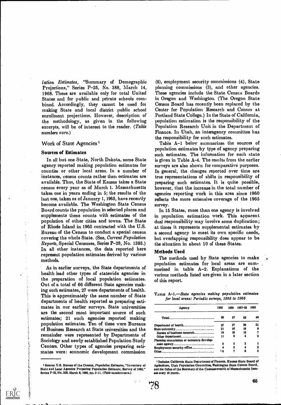
lation Estimates, "Summary of DemographicProjections," Series P-25, No. 388, March 14,1968. These are available only for total UnitedStates and for public and private schools com-bined. Accordingly, they cannot be used formaking State and local district public schoolenrollment projections. However, description ofthe methodology, as given in the followingexcerpts, will be of interest to the reader. (Tablenumbers ours.)
Work of State Agencies 1
Sources of EstimatesIn all but one State, North Dakota, some State
agency reported making population estimates forcounties or other local areas. In a number ofinstances, census counts rather than estimates areavailable. Thus, the State of Kansas takes a Statecensus every year as of March 1. Massachusettstakes one in years ending in 5; the results of thelast one, taken as of January 1,1965, have recentlybecome available. The Washington State CensusBostrd counts the population in selected places andsupplements these counts with estimates of thepopulation of other cities and towns. The Stateof Rhode Island in 1965 contracted with the U.S.Bureau of the Census to conduct a special censuscovering the whole State. (See, Current PopulationReports, Special Censuses, Series P-28, No. 1393.)In all other instances, the data reported hererepresent population estimates derived by variousmethods.
As in earlier surveys, the State departments ofhealth lead other types of statewide agencies inthe preparation of local population estimates.Out of a total of 66 different State agencies mak-ing such estimates, 27 were departments of health.This is approximately the same number of Statedepartments of health reported as preparing esti-mates in our earlier surveys. State universitiesare the second most important source of suchestimates; 21 such agencies reported makingpopulation estimates. Ten of these were Bureausof Business Research at State universities and theremainder were represented by Departments ofSociology and newly established Population StudyCenters. Other types of agencies preparing esti-mates were: economic development commission
Source: U.S. Bureau of tho Census, Population Eatimaies, "Inventory ofState and Local Agencks Preparing Population Estimate, Survey of 1965,"Series P-25, No. 328, March 8, 1966, pp. 2-11. (Table number. ours.)
(6), employment security commissions (4), Stateplanning commissions (3), and other agencies.These agencies include the State Census Boardsin Oregon and Washington. (The Oregon StateCensus Board has recently been replaced by theCenter for Population Research and Census atPortland State College.) In the State of California,population estimation is the responsibility of thePopulation Research Unit in the Department ofFinance. In Utah, an interagency committee h asthe responsibility for such estimates.
Table A-1 below summarizes the sources ofpopulation estimates by type of agency preparingsuch estimates. The information for each stateis given in Table A-4. The results from the earliersurveys are also shown for comparative purposes.In general, the changes reported over time aretrue representations of shifts in responsibility ofpreparing such estimates. It is quite possible,however, that the increase in the total number ofagencies reporting work in this area since 1960reflects the more extensive coverage of the 1965survey.
In 15 States, more than one agency is involvedin population estimation work. This apparentdual responsibility may involve some duplication;at times it represents supplemental estimates bya second agency to meet its own specific needs,but overlapping responsibility does appear to bethe situation in about 10 of these States.
Methods UsedThe methods used by State agencies to make
population estimates for local areas are stun-marized in table A-2. Explanations of thevarious methods listed are given in a later sectionof this report.
TABLE A-1.State agencies making population estimatesfor local areas: Periodic surveys, 1956 to 1966
Agency 1965 1960 1957-58 1955
Total 66 67 62 46
Department of health 27 27 30 31
State university 21 16 19 9
Bureau of business research 10 10 15 7
Other department 11 6 4 2
Planning commission or oconomlo dovolopmont agency 9 5 3 1
Employment security Wilco 4 2 4 2
Other 1 5 7 6 3
Includes California State Department of Finance, Kansas State Board ofAgriculture, Utah Population Committee, Washington State Census Board,and tho Office of tho Secretary of the Commonwealth of Massachusetts (cen-sus every 10 years).
65
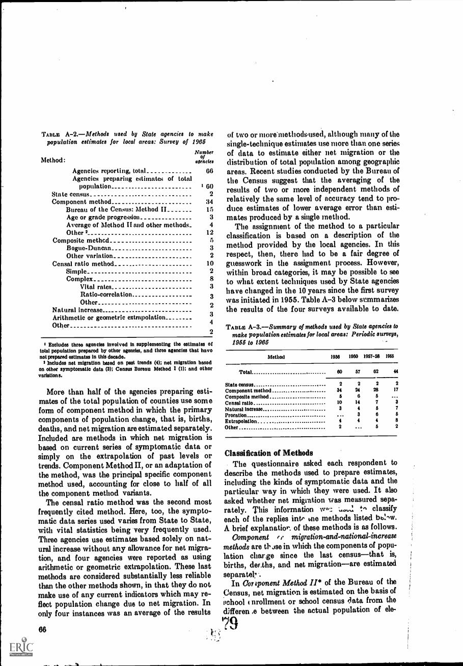
TABLE A-2.Methods used by State agencies to makepopulation estimates for local areas: Survey of 1965
Method:
Agencies reporting, totalAgencies preparing estimates of total
populationState censusComponent method
Bureau of the Census: Method IIAge or grade progressionAverage of Method II and other methods..Other 2
Composite methodBogue-DuncanOther variation
Censal ratio method_SimpleComplex
Vital ratesRatio-correlationOther
Natural increaseArithmetic or geometric extrapolationOther
Numberof
agencies
66
3 602
:34
1534
12532
10283
3
234
2
Excludes three agonclos involved in supplementing the estimates oftotal population proparod by othor agencies, and throe agencies that havonot prepared estimates in this decade.
I Includes not migration based on past trendson other symptomatic data (3); Census Bureau Method I (1): and othorvariation s.
(4); not migration basod
More than half of the agencies preparing esti-mates of the total population of counties use someform of component method in which the primarycomponents of population change, that is, births,deaths, and net migration are estimated separately.Included are methods in which net migration isbased on current series of symptomatic data orsimply on the extrapolation of past levels ortrends. Component Method II, or an adaptation ofthe method, was the principal specific componentmethod used, accounting for close to half of allthe component method variants.
The censal ratio method was the second mostfrequently cited method. Here, too, the sympto-matic data series used varies from State to State,with vital statistics being very frequently used.Three agencies use estimates based solely on nat-ural increase without any allowance for net migra-tion, and four agencies wore reported as usingarithmetic or geometric extrapolation. These lastmethods are considered substantially less reliablethan the other methods shown, in that they do notmake use of any current indicators which may re-flect population change due to net migration. Inonly four instances was an average of the ragults
66
of two or moramethods,used, although many of thesingle-technique estimates use more than one seriesof data to estimate either net migration or thedistribution of total population among geographicareas. Recent studies conducted by the Bureau ofthe Census suggest that the averaging of theresults of two or more independent methods ofrelatively the same level of accuracy tend to pro-duce estimates of lower average error than esti-mates produced by a single method.
The assignntent of the method to a particularclassification is based on a description of themethod provided by the local agencies. In thisrespect, then, there had to be a fair degree ofguesswork in the assignment process. However,within broad categories, it may be possible to seeto what extent techniques used by State agencieshave changed in the 10 years since the first surveywas initiated in 1955. Table A-3 below summarizesthe results of the four surveys available to date.
TABLE A-3.Summary of methods used by State agencies tomake population estimates for local areas: Periodic surveys,1955 to 1965
Method 1956 1960 1957-58 1955
Total 60 57 62 44
State census 2 2 2 2
Component method 34 24 28 17
Composite method 5 6 5 ...Censal ratio. 10 14 7 3
Natural increase 3 4 5 7
Proration ... 3 6 5
Extrapolation 4 4 4 8
Other 2 ... 5 2
Classification of MethodsThe questionnaire asked each respondent to
describe the methods used to prepare estimates,including the kinds of symptomatic data and theparticular way in which they were used. It alsoasked whether net migration was measured sepa-rately. This information I.-, classifyeach of the replies infr une methods listed bb:-.w.A brief explanation of these methods is as follows.
Component migration-and-national-increasemethods are th jee in which the components of popu-lation charge since the last censusthat is,
births, der.ths, and net migrationare estimatedseparatel7 .
In Cot' tponent Method I I* of the Bureau of theCensus, net migration is estimated on the basis ofschool nrollment or school census aata from the
differen ,f3 between the actual population of ele-
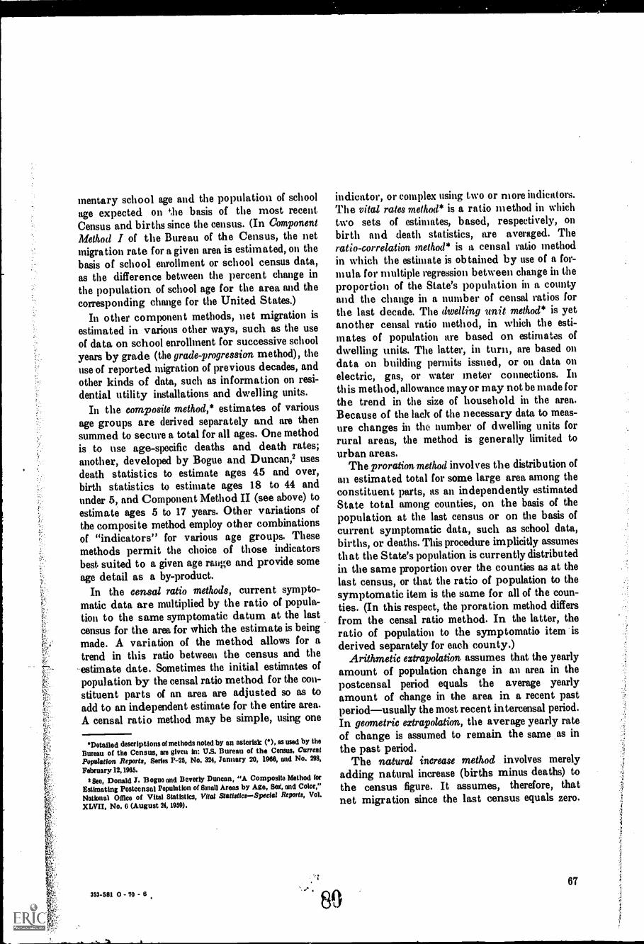
mentary school age and the population of schoolage expected on *lie basis of the most recentCensus and births since the census. (In Component
Method I of the Bureau of the Census, the netmigration rate for a given area is estimated, on thebasis of school enrollment or school census data,as the difference between the percent change inthe population of school age for the area and thecorresponding change for the United States.)
In other component methods, net migration isestimated in various other ways, such as the useof data on school enrollment for successive school
years by grade (the grade-progression method), theuse of reported migration of previous decades, andother kinds of data, such as information on resi-dential utility installations and dwelling units.
In the composite method,* estimates of variousage groups are derived separately and are thensummed to secure a total for all ages. One methodis to use age-specific deaths and death rates;another, developed by Bogue and Duncan,2 usesdeath statistics to estimate ages 45 and over,birth statistics to estimate ages 18 to 44 andunder 5, and Component Method II (see above) toestimate ages 5 to 17 years. Other variations of
the composite method employ other combinationsof "indicators" for various age groups. Thesemethods permit the choice of those indicatorsbests suited to a given age rauge and provide someage detail as a by-product.
In the censal ratio methods, current sympto-matic data are multiplied by the ratio of popula-tion to the same symptomatic datum at the lastcensus for the area for which the estimate is beingmade. A variation of the method allows for atrend in this ratio between the census and the-estimate date. Sometimes the initial estimates of
population by the censal ratio method for the con-stituent parts of an area are adjusted so as toadd to an independent estimate for the entire area.A censal ratio method may be simple, using one
'Detailed descriptions of methods noted by an asterisk (), as used by the
Bureau of the Census, are given in: U.S. Bureau of the Census, CurrentPopulation Reports, Series P-25, No. 324, January 20, 1966, and No. 298,
February 12, 1965.I See, Donald J. Bogue and Beverly Duncan, "A Composite Method for
Estimating Postcensal Population of Small Areas by Age, See, and Color,"
National Office of Vital Statistics, Vital StatisticsSpecial Reports, Vol.
XLVII, No. 6 (August 24, 1959).
353-581 0-70 - 6
indicator, or complex using two or more indicators.The vital rates method* is a ratio method in whichtwo sets of estimates, based, respectively, onbirth and death statistics, are averaged. Theratio-correlation method* is a censal ratio methodin which the estimate is obtained by use of a for-mula for multiple regression between change in theproportion of the State's population in a countyand the change in a number of censal ratios forthe last decade. The dwelling unit method* is yetanother censal ratio method, in which the esti-mates of population are based on estimates ofdwelling units. The latter, in turn, are based ondata on building permits issued, or on data onelectric, gas, or water meter connections. Inthis method, allowance may or may not be made forthe trend in the size of household in the area.Because of the lack of the necessary data to meas-ure changes in the number of dwelling units forrural areas, the method is generally limited tourban areas.
The proration method involves the distribution ofan estimated total for some large area among theconstituent parts, as an independently estimatedState total among counties, on the basis of thepopulation at the last census or on the basis ofcurrent symptomatic data, such as school data,births, or deaths. This procedure implicitly assumesthat the State's population is currently distributedin the same proportion over the counties as at thelast census, or that the ratio of population to thesymptomatic item is the same for all of the coun-ties. (In this respect, the proration method differsfrom the censal ratio method. In the latter, theratio of population to the symptomatio item isderived separately for each county.)
Arithmetic extrapolation assumes that the yearlyamount of population change in an area in thepostcensal period equals the average yearlyamount of change in the area in a recent pastperiodusually the most recent intercensal period.In geometric extrapolation, the average yearly rateof change is assumed to remain the same as inthe past period.
The natural increase method involves merelyadding natural increase (births minus deaths) tothe census figure. It assumes, therefore, thatnet migration since the last census equals zero.
8067
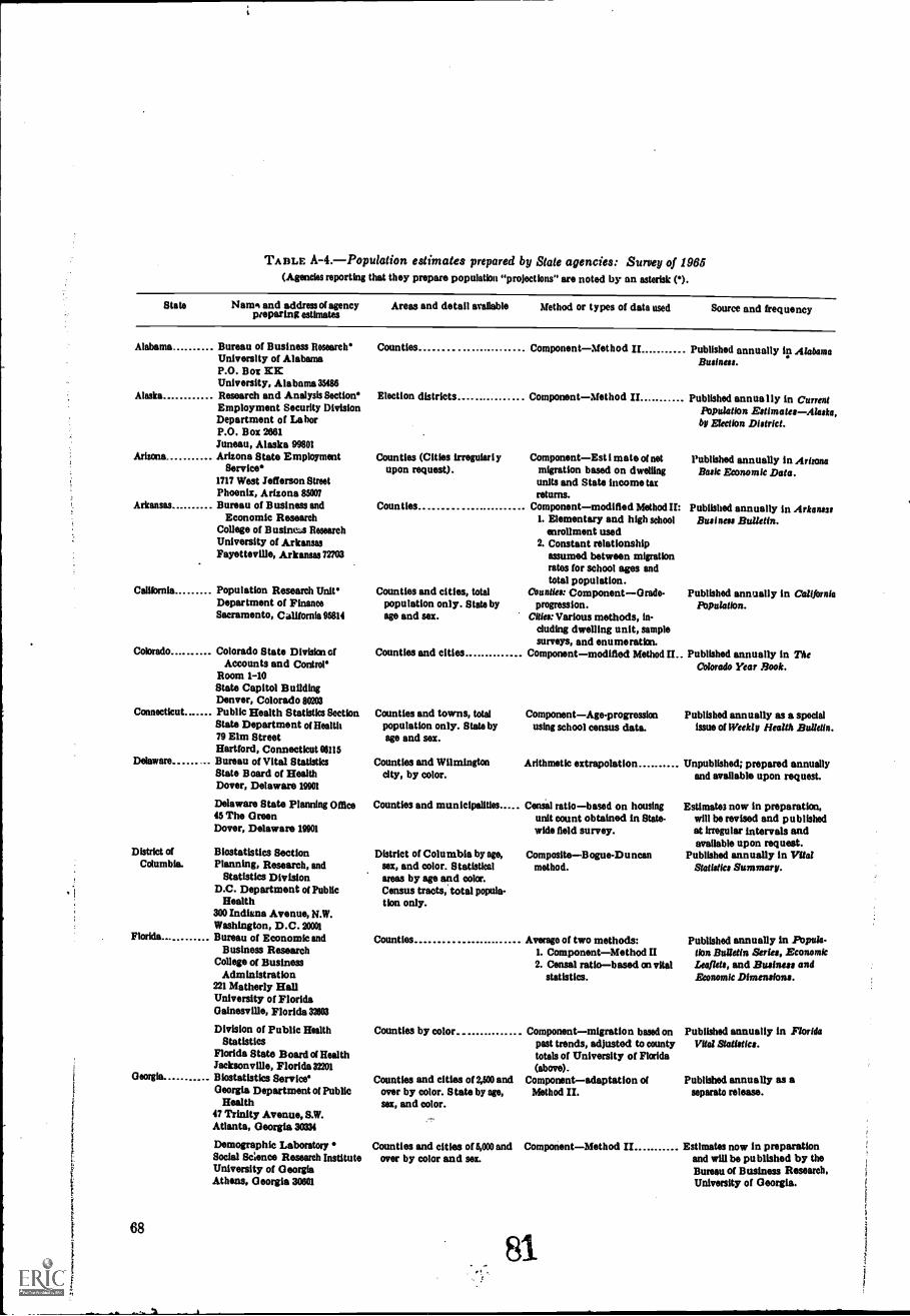
TABLE A-4.Populalion estimates prepared by State agencies: Survey of 1965(Agencies reporting that they prepare population "projections" are noted by an asterisk (9.
State Namq and address of agencypreparing estimates
Areas and detail available Method or types of data used Source and frequency
Alabama Bureau of Business Research*University of AlabamaP.O. Box MrUniversity, Alabama 35486
Alaska Research and Analysis Section*Employment Security DivisionDepartment of LaborP.O. Box 2661Juneau, Alaska 99801
Arizona Arizona State EmploymentService*
1717 West Jefferson StreetPhoenix, Arizona 85007
Arkansas Bureau of Business andEconomic Research
College of Businez..1 ResearchUniversity of ArkansasFayetteville, Arkansas 72703
California Population Research Unit*Department of FinanceSacramento, California 95814
Colorado. Colorado State Division ofAccounts and Control*
Room 1-10State Capitol BuildingDenver, Colorado 80203
Connecticut Public Health Statistics SectionState Department of Health79 Elm StreetHartford, Connecticut 06115
Delaware Bureau of Vital StatisticsState Board of HealthDover, Delaware 19901
Delaware State Planning Office45 The GreenDover, Delaware 19901
District of Blostatistics SectionColumbia. Planning, Research, and
Statistics DivisionD.C. Department of Public
Health300 Indiana Avenue, N.W.Washington, D.C. 20001
Florida Bureau of Economic andBusiness Research
College of BusinessAdministration
221 Matherly HallUniversity of FloridaGainesville, Florida 32603
Division of Public HealthStatistics
Florida State Board of HealthJacksonville, Florida 32201
Georgia. Biostatistics Service*Georgia Department of Public
Health47 Trinity Avenue, S.W.Atlanta, Georgia 30334
Demographic LaboratorySocial Science Research InstituteUniversity of GeorgiaAthens, Georgia 30601
68
Counties ... ComponentMethod II .. Published annually in AlabamaBusiness.
Election districts ComponentMethod II
Counties (Cities irregularl y ComponentEst 1 mate of netupon request). migration based on dwelling
units and State income taxreturns.
Counties Componentmodified Method II:1. Elementary and high school
enrollment used2. Constant relationship
assumed between migrationrates for school ages andtotal population.
Counties: Component-0 rade-progression.
Cities: Various methods, in-chiding dwelling unit, samplesurveys, and enumeration.
Counties and cities Componentmodified Method II..
Counties and cities, totalpopulation only. State byage and sex.
Counties and towns, totalpopulation only. State byage and sex.
Counties and Wilmingtoncity, by color.
Counties and municipalities...
District of Columbia by age,sex, and color. Statisticalareas by age and color.Census tracts, total popula-tion only.
Counties
Counties by color.
Counties and cities of 2,500 andover by color. State by age,sex, and color.
Counties and cities of 5,000 andover by color and sex.
ComponentAge-progressionusing school census data.
Published annually in CurrentPopulation EstimatesAlada,by Election District.
Published annually in ArizonaBask Economic Data.
Published annually in ArkaneasBusiness Bulletin.
Published annually in CaliforniaPopulation.
Published annually in TheColorado Year Book.
Published annually as a specialissue of Weekly Health Bulletin.
Arithmetic extrapolation Unpublished; prepared annuallyand available upon request.
Censel ratiobased on housingunit count obtained in State-wide field survey.
CompositeBogue-Duncanmethod.
Average of two methods:1. ComponentMethod II2. Censal ratiobased on vital
statistics.
Componentmigration based onpast trends, adjusted to countytotals of University of Florida(above).
Componentadaptation ofMethod U.
Estimates now in preparation,will be revised and publishedat irregular intervals andavailable upon request.
Published annually in VitalStatistics Summary.
Published annually in Popula-tion Bulletin Series, EconomicLeaflets, and Business andEconomic Dimensions.
Published annually in FloridaVital Statistics.
Published annually as aseparato release.
ComponentMethod II Estimates now in preparationand will be published by theBureau of Business Research.University of Georgia.
81
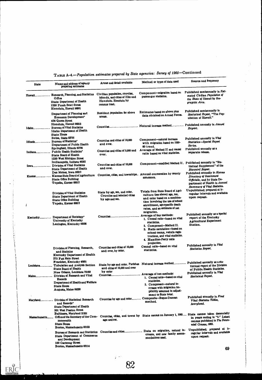
TABLE A-4.Population estimates prepared by State agencies: Survey of 1966Continued
State Name and address of agencypreparing estimates
Hawaii Research, Planning, and StatisticsOffice
State Department of Health1250 Punch Bowl StreetHonolulu, Hawaii 96801
Department of Planning andEconomic Development'
426 Queen StreetHonolulu, Hawaii 96813
Idaho Bureau of Vital StatisticsIdaho Department of HealthState HouseBoise, Idaho 83701
Illinois Bureau of Statistics'Department of Public HealthSpringfield, Illinois 62706
Indiana Public Health Statistics'State Board of Health1330 West Michigan StreetIndianapolis, Indiana 46202
Iowa. Division of Vital StatisticsState Department of HealthDes Moines, Iowa 50319
Kansas Kansas State Board of AgricultureState Office BuildingTopeka, Kansas 66612
D ivision of Vital StatisticsState Department of HealthState Office BuildingTopeka, Kansas 66612
Kentucky Department of Sociology'University of KentuckyLexington, Kentucky 40506
D ivision of Planning, Research,and Statistics
Kentucky Department of Health275 Fast Main StreetFrankfort, Kentucky 40601
Louisiana Tabulation and Analysis SectionState Board of HealthNew Orleans, Louisiana 70160
Maine Division of Research and VitalRecords
Department of Health and WelfareState HouseAugusta, Maine 09330
Maryland Division of Statistical Researchand Records'
State Department of Health301 West Preston StreetBaltimore, Maryland 21201
Massachusetts Office of tho Secretary of the Com-monwealth
State HouseBoston, Massachusetts 02133
Bureau of Research and StatisticsState Department of Commerce
and Development150 Causeway StreetBoston, Massachusetts 02114
Areas and detail available Method or types of data used Source and frequency
Civilian population, counties,islands, and cities of Hilo andHonolulu. Honolulu bycensus tract.
Resident population for aboveareas.
Counties
Counties and cities of 10,000and over.
Counties and cities of 5,000 andver.
Counties and cities of 10,000and over.
Counties, cities, and townships.
State by age, sex, and color.Counties and selected citiesby age and sex.
Counties
Counties and cities of 10,000and over, by color.
State by age and color. Parishesand cities of 10,000 and overby color
Counties
Counties by ago and color
Counties, cities, and towns byage and sax.
Counties and cities
82
Componentmigration based onpassenger statistics.
Estimates based on above plusdata obtained on Armed Forces.
Natural increase method
Componentnatural increasewith migration based on 1950-60 trend.
Average of Method H and comalratio based on vital statistics.
Componentmodified Method If.
Annual enumeration by countyaSseSSOIS.
Totals from State Board of Agri-culture (see above) age, sox,and color based on a combina-tion involving the use of schoolenrollment, age-specific deathrates, and an estimate of net
igration.Average of four methods:
1. Censal ratiobased on vitalstatistics.
2. ComponentMethcd H.3. Ratio correlationbased on
school census, vehicle regis-trations, and vital statistics.
4. Hamliton-Perry ratioprojection.
Censal ratiobased on vitalstatistics.
Natural increase method
Average of two methods:1. Censal ratiobased on vital
statistics.2. Componentnatural in-
crease with migration im-plicitly assumed in adjust-ment to State total.
CompositeBogue-Duncanmethod.
State census on January 1, 1965
Data on migration, natural in-crease, and new family accom-modations used.
Published semiannually in Esti-mated Civilian Population ofthe State of Hawaii by Geo-graphic Area.
Published semiannually inStatistical Report, "The Pop-ulation of Hawaii."
Published annually in AnnualReport.
Published annually in VitalStatisticsSpecial ReportSeries.
Published annually as aseparate release.
Published annually In "Sta-tistical Supplement" of thoBiennial Report.
Published annually in KansasDirectory of GovernmentOfficials, and by State De-partment of Health in AnnualSummary of Vital Statistics.
Unpublished; prepared at ir-regular intervals and availableupon request.
Published annually as a specialreport of the KontuckyAgricultural ExperimentStation.
Published annually in VitalStatistics Report.
Published annually as a sta-tistical report of the Divisionof Public Health Statistics.
Published annually in VitalStatistical Report.
Published annually in FinalVital Statistics Tables,Maryland.
State census taken decenniallyin years ending in "5." Latestcensus published In The Decen-
nial Census, 1965.
Unpublished; prepared at ir-regclar intervals and availableupon request.
69
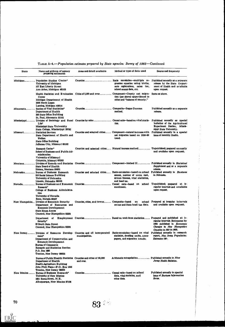
TABLE A-4.Population estimates prepared by State agencies: Survey of 1965Continued
State Name and address of agencypreparing estimates
Areas and detail available Method or types of data used Source and frequency
Michigan Population Studies Center*University of Michigan527 East Liberty StreetAnn Arbor, Michigan 48103
Health Statistics and EvaluationCenter
Michigan Department of Health3500 North LoganLansing, Michigan 43914
M innesot a Section of Vital Statistics*Department of Health350 State Office BuildingSt. Paul, Minnesota 55101
Mississippi Division of Sociology and RuralLife*
Mississippi State UniversityState College, Mississippi 39782
M issouri Statistical ServicesState Department of Health and
WelfareState Office BuildingJefferson City, Missouri 85102
Research Center*School of Business and Public Ad-
ministrationUniversity of MissouriColumbia, Missouri 85202
Montana Division of Records and StatisticsState Board of HealthHelena, Montana 59801
Nebraska Bureau of Business Research310 Social Science BuildingUniversity of NebraskaLincoln, Nebraska 88503
Nevada Bureau of Business and EconomicResearch*
College of Business AdminIstra-tion
University of NevadaReno, Nevada 89507
New Hampshire Division of Economic SecurityDepartment of Resources and
Economic DevelopmentState House AnnexConcord, New Hampshire 03301
Department of EmploymentSecurity*
32 South Main StreetConcord, New Hampshire 03301
New Jersey Division of Resource Develop-ment*
Department of Conservation andEconomic Development
Bureau of CommerceResearch and Statistics SectionP.O. Box 1889Trenton, New Jersey 08625
Bureau of Public Health Statistics Counties and cities of 50,000Department of Health and over.Health-Agriculture BuildingJohn Pitch PlazaP.O. Box 1540Trenton, New Jersey 08625
New Mexico Bureau of Business Research*University of New Mexico1821 Roma Street, N.E.Albuquerque, New Mexico 87108
Counties Ratio correlation--multiple re-gression equation using births,auto registrations, sales tax,school census data, etc.
Cities of 2,500 and over ComponentCounty not migra-tion (per above) apportioned tocities and "balance of county."
Counties CompositeBogue-Duncanmethod.
Counties by color Censal ratiobased on vital statis-tics.
Counties and selected cities Componentnatural increase withnet migration based on 1950-60trend.
Counties and selected cities.... Natural increase method
Counties ComponentMethod II
Counties and selected cities Ratio-correlationbased on schoolcensus, number of votes cast,drivers licenses, vital statistics,and head tax.
Counties Consal ratiobased on schoolenrollment.
Published annually as a separaterelease by the State Depart-ment of Health and availableupon request.
Same as above.
Published annually as a separaterelease.
Published annually as specialbulletins of the AgriculturalExperiment Station, Missls-sippi State University.
Published annually in a specialissue of monthly Health.
Unpublished; prepared annuallyand available upon request.
Published annually in StatisticalSupplement and as a separaterelease.
Published annually in Businessin Nebraska.
Unpublished; prepared at ir-regular intervals and availableupon request.
Counties, cities, and towns Compositebased on school Prepared at irregular intervalscensus and State head tax data. and available upon request.
Counties Basetron work-foree statistics
Counties and all incorporated Ratio-correlationbased on vitalmunicipalities, statistics, dwelling units, news-
papers, and migration trends.
70
Arithmetic extrapolation
Counties Censal ratiobased on schooldata, vital statistics, andother data.
Prepared and published at ir-regular intervals. Estimates for1964 published in EconomicChanges in New HampshireCounties in 195I to 1961.
Published annually in researchreport, New Jersey PopulatiouEstimates IX-.
Publlshed annually In NewJersey Health Statistics.
Published annually in specialissue of Dulness InformationSeries.
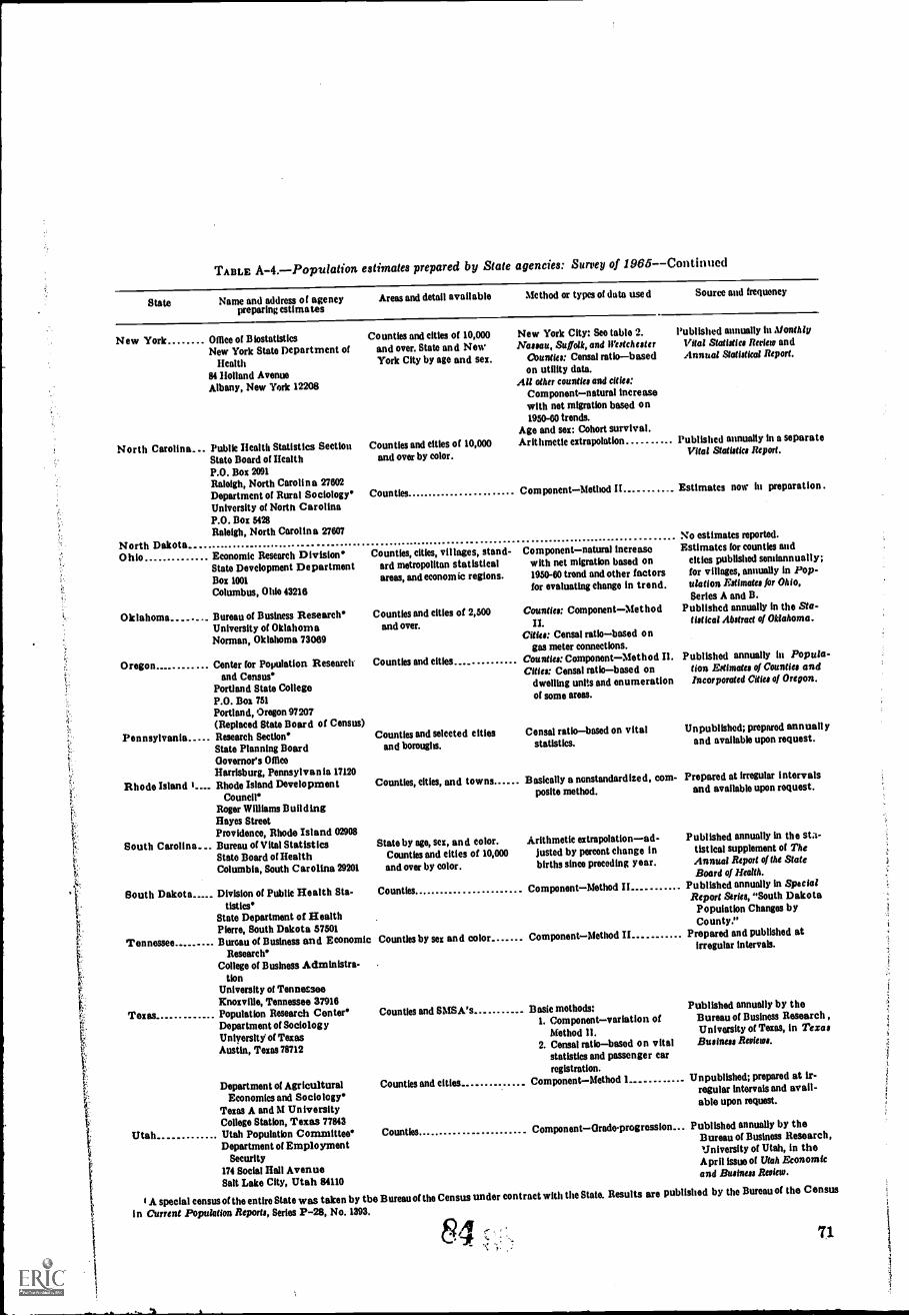
TABLE A-4.Populalion estimates prepared by State agencies: Survey of/965Continued
State Name and address of agencypreparing estimates
Areas and detail available Method or types of data used Source and frequency
New York Office of BlostatisticsNew York State Department of
Health84 Holland AvenueAlbany, New York 12208
North Carolina_ Public Health Statistics SectionState Board of HealthP.O. Box 2091Raleigh, North Carolina 27602Department of Rural Sociology' CountiesUniversity of North CarolinaP.O. Box 5428Raleigh, North Carolina 27607
North Dakota.
Counties and cities of 10,000and over. State and NowYork City by age and sex.
Counties and cities of 10,000and over by color.
Ohio Economic Research Division'State Development DepartmentBox 1001Columbus, Olde 43216
Oklahoma Bureau of Business Research'University of OklahomaNorman, Oklahoma 73069
Oregon Center for Population Researchand Census'
Portland State CollegeP.O. Box 751Portland, Oregon 97207(Replaced State Board of Census)
Pennsylvania Research Section'State Planning BoardGovernor's OfficeHarrisburg, Pennsylvania 17120
Rhode Island 1 Rhode Island DevelopmentCouncil'
Roger Williams BuildingHayes StreetProvidence, Rhode Island 02908
South Carolina Bureau of Vital StatisticsState Board of HealthColumbia, South Carolina 29201
South Dakota Division of Public Health Sta-tistics'
State Department of HealthPierre, South Dakota 57501
Tennessee Bureau of Business and EconomicResearch'
College of Business Administra-tion
University of TennesseeICnoxville, Tennessee 37916
Texas Population Research Center'Department of SociologyUnlyersit V of TexasAustin, Texas 78712
Department of AgriculturalEconomies and Sociology'
Texas A and M UniversityCollege Station, Texas 77843
Utah Utah Population Committee°Department of Employment
Security174 Social Hall AvenueSalt Lake City, Utah 84110
Counties, cities, villages, stand-ard metropolitan statisticalareas, and econom ic regions.
Counties and cities of 2,500and over.
Counties and cities
Counties and selected e Riesand boroughs.
Counties, cities, and towns
State by ago, sex, and color.Counties and cities of 10,000and over by color.
Counties
Counties by sex and color
Counties and SMSA's
Counties and cities
Counties
New York City: See table 2.Nassau, Suffolk, and Westchester
Counties: Consul ratiobasedon utility data.
All other counties and cities:Componentnatural Increasewith net migration based on1950-60 trends.
Ago and sex: Cohort survival.Arithmetic extrapolation
Published annually in MonthlyVita( Statistics Review andAnnual Statistical Report.
Published annually in a separateVital Statistics Report.
ComponentMethod Il Estimates now in preparation.
Componentnatural Increasewith net migration based on1950-60 trend and other factorsfor evaluating change in trend.
Counties: ComponentMethod
Censal ratiobased ongas meter connections.
Counties: ComponentMethod II.Censal ratiobased on
dwelling units and enumerationor some areas.
Censal ratiobased on vitalstatistics.
No estimates reported.Estimates for counties and
cities published semiannually;for villages, annually in Pop-ulation Estimates for Ohio,Series A and B.
Published annually in the Sta-tistical Abstract of Oklahoma.
Published annually in Popula-tion Estimates of Counties andIncorporated Cities of Oregon.
Unpublished; prepared annuall yand available upon request.
Basically a nonstandardized, com- Prepared at irregular intervals
posite method, and available upon request.
Arithmetic extrapolationad-justed by percent change inbirths since preceding year.
ComponentMethod II
ComponentMethod
Basic methods:1. Componentvariation of
Method 11.2. Camel ratiobased on vital
statistics and passenger carregistration.
ComponentMethod I Unpublished; prepared at Ir-regular intervals and avail-able upon request.
Published annually in the sta-tistical supplement of TheAnnual Report of the StateBoard of Health.
Published annually in SpecialReport Series, "South DakotaPopulation Changes byCounty."
Prepared and Published atirregular intervals.
Published annually by theBureau of Business Research ,University of Texas, in TexasBusiness Reviews.
ComponentGrade-progression... Published annually by theBureau of Business Research,University of Utah, in theApril issue of Utah Economicand Business Review.
A special census of the entire State was taken by the Bureau or the Census under contract with the State. Results aro published by the Bureau of the Census
in Current Population Reports, Series P-28, No. 1393.
71
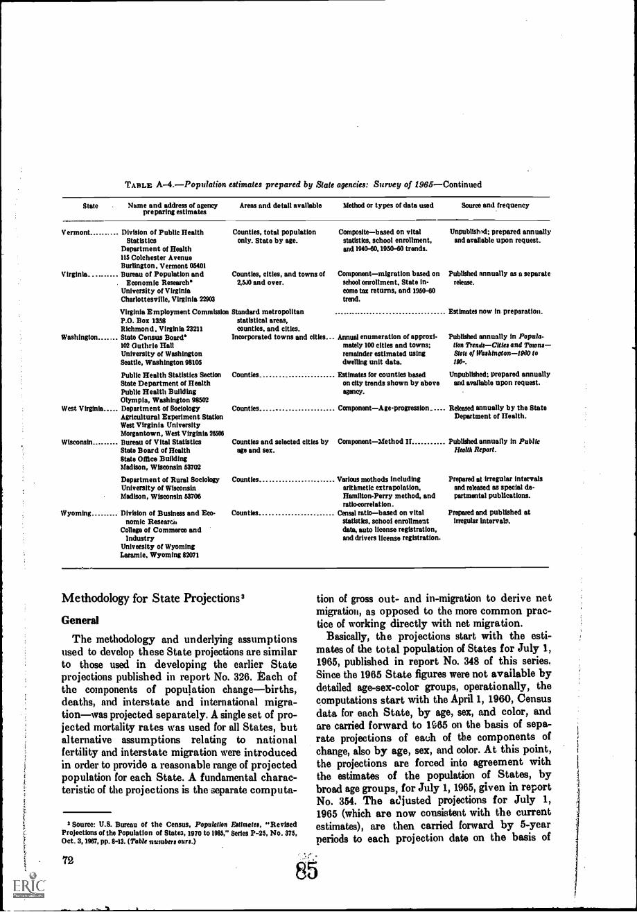
TABLE A-4.Population estimates prepared by State agencies: Survey of 1965Continued
State Name and address of agencypreparing estimates
Areas and detail available Method or types of data used Source and frequency
Vermont Division of Public Health Counties, total populationStatistics only. State by age.
Department of Health115 Colchester AvenueBurlington. Vermont 05401
Virginia. Bureau of Population and Counties, cities, and towns ofEconomic Research' 2,5J0 and over.
University of VirginiaCharlottesville, Virginia 22903
Virginia Employment Commission Standard metropolitanP.O. Box 1358 statistical areas,Richmond, Virginia 23211 counties, and cities.
Washington State Census Board' Incorporated towns and cities...102 Guthrie HallUniversity of WashingtonSeattle, Washington 98105
Public Health Statistics SectionState Department of HealthPublic Health BuildingOlympia, Washington 98502
West Virginia Department of SociologyAgricultural Experiment StationWest Virginia UniversityMorgantown, West Virginia 28508
Wisconsin Bureau of Vital StatisticsState Board of HealthEttate 01 Ree BuildingMadison, Wisconsin 53702
Department of Rural SociologyUniversity of WisconsinMadison, Wisconsin 53708
Wyoming Division of Business and Eco-nomic Researca
College of Commerce andIndustry
University of WyomingLaramie, Wyoming 82071
Compositebased on vitalstatistics, school enrollment,and 1940-80, 1950-80 trends.
Unpublishld: prepared annuallyand available upon request.
Componentmigration based on Published annually as a separateschool enrollment, State in- release.come tax returns, and 1950-00trend.
Annual enumeration of approxi-mately 100 cities and towns:remainder estimated usingdwelling unit data.
Counties Estimates for counties basedon city trends shown by aboveagency.
Counties ComponentAge-progression....
Counties and selected cities byage and sex.
Counties
Counties
Estimates now in preparation.
Published annually in Popula-tion TrendsCities and TownsStote of Washington-19E10 to
Unpublished: prepared annuallyand available upon request.
. Released annually by the StateDepartment of Health.
ComponentMethod II
Various methods includingarithmetic extrapolation,Hamilton-Perry method, andratio-correlation.
Censal ratiobased on vitalstatistics, school enrollmentdata, auto license registration,and drivers license registration.
Published annually in PublicHealth Report.
Prepared at irregular intervalsand released as special de-partmental publications.
Prepared and published atirregular intervals.
Methodology for State Projections3
General
The methodology and underlying assumptionsused to develop these State projections are similarto those used in developing the earlier Stateprojections published in report No. 326. Each ofthe components of population changebirths,deaths, and interstate and international migra-tionwas projected separately. A single set of pro-jected mortality rates was used for all States, butalternative assumptions relating to nationalfertility and interstate migration were introducedin order to provide a reasonable range of projectedpopulation for each State. A fundamental charac-teristic of the projections is the separate compute-
3 Source: U.S. Bureau of the Census, Population Estimates, "RevisedProjections of the Population of Staten, 1970 to 1985," Series P-25, No. 375,Oct. 3, 1987, pp. 8-13. (Table numbers ours.)
72
tion of gross out- and in-migration to derive netmigration, as opposed to the more common prac-tice of working directly with net migration.
Basically, the projections start with the esti-mates of the total population of States for July 1,1965, published in report No. 348 of this series.Since the 1965 State figures were not available bydetailed age-sex-color groups, operationally, thecomputations start with the April 1, 1960, Censusdata for each State, by age, sex, and color, andare carried forward to 1c;65 on the basis of sepa-rate projections of each of the components ofchange, also by age, sex, and color. At this point,the projections are forced into agreement withthe estimates of the population of States, bybroad age groups, for July 1, 1965, given in reportNo. 354. The Ousted projections for July 1,1965 (which are now consistent with the currentestimates), are then carried forward by 5-yearperiods to each projection date on the basis of
85
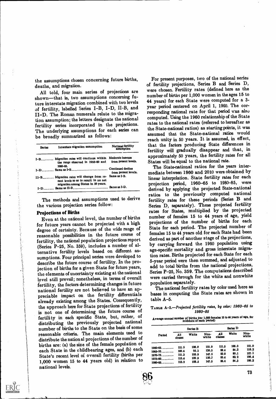
1
the assumptions chosen concerning future births,deaths, and migration.
All told, four main series of projections areshown-that is, two assumptions concerning fu-ture interstate migration combined with two levelsof fertility, labelled Series I-B, I-D, II-B, andII-D. The Roman numerals relate to the migra-tion assumption; the letters designate the nationalfertility series incorporated in the projections.The underlying assumptions for each series canbe broadly summarized as follows:
Series Interstate Migration assumption National fertilityassumption
I-B Migration rates will continue withinthe range observed in 1955-60 and1960-65.
I-D Same as I-13
II-B Migration rates will change from re-cent levels so as to result in no netmigration among States in 50 years.
I-D Same as II-B
Moderate increasefrom present levels.
Continued declinefrom present levels.
Same as I-B.
Same as I-D.
The methods and assumptions used to derivethe various projection series follow:
Projections of BirthsEven at the national level, the number of births
for future years cannot be projected with a highdegree of certainty. Because of the wide range ofreasonable possibilities in the future course of
fertility, the national population projections report(Series P-25, No. 359), includes a number of al-ternative fertility levels based on different as-sumptions. Four principal series were developed todescribe the future course of fertility. In the pro-jection of births for a given State for future years,the elements of uncertainty existing at the nationallpvel still prevail; nonetheless, in terms of overallfertility, the factors determining changes in futurenational fertility are not believed to have an ap-preciable impact on the fertility differentialsalready existing among the States. Consequently,the approach here for State projections of fertilityis not one of determining the future course offertility in each specific State, but, rather, ofdistributing the previously projected nationalnumber of births to the State on the basis of somereasonable criteria. The main elements used todistribute the nation al projections of the number ofbirths are: (a) the size of the female population ofeach State in the childbearing ages, and (b) eachState's recent level of overall fertility (births per1,000 women 15 to 44 years old) in relation tonational levels.
For present purposes, two of the national seriesof fertility projections, Series B and Series D,were chosen. Fertility rates (defined here as thenumber of births per 1,000 women in the ages 15 to44 years) for each State were computed for a 3-year period centered on April 1, 1960. The cor-responding national rate for that period was alsocomputed. Using the 1960 relationship of the Staterates to the national rates (referred to hereafter asthe State-national ratios) as starting points, it wasassumed that the State-national ratios wouldreach unity in 50 years. It is assumed, in effect,that the factors producing State differences infertility will gradually disappear and that, inapproximately 50 years, the fertility rates for allStates will be equal to the national rate.
The State-national ratios for the years inter-mediate between 1960 and 2010 were obtained bylinear interpolation. State fertility rates for eachprojection period, 1960-65 to 1980-85, werederived by applying the projected State-nationalratios to the previously computed nationalfertility rates for these periods (Series B andSeries D, separately). These projected fertilityrates for States, multiplied by the projectednumber of females 15 to 44 years of age, yieldprojections of the number of births for eachState for each period. The projected number offemales 15 to 44 years old for each State had beenderived as part of another stage of the projections,by carrying forward the 1960 population usingage-specific mortality and gross interstate migra-tion rates. Births projected for each State for each5-year period were then summed, and adjusted toadd to total births from the national projections,Series P-25, No. 359. The computations describedwere carried through for the white and nonwhitepopulation separately.
The national fertility rates by color used here asbases in computing the State rates are shown intable A-5.
TABLE A-5.-Projecied fertility rates, by color: 1960-66 to1980-86
Average annual number of births per 1,000 females 15 to 44 years of age, formiddate of each period)
Series B Series D
Period All White Non- All White Non-cbsses white classes white
196045 111.5 106.0 151.9 111.5 106.0 151.9
1965-70 100.4 95.2 136.5 88.4 84.2 118.2
1970-75 111.3 105.9 147.5 83.6 80.1 107.1
1975-80 115.4 109.9 150.7 85.4 82.2 106.4
1980-85 113.9 108.5 147.5 86.4 84.3 106.2
8673
Projections of DeathOne set of age-sex-color-specific mortality rates
was used for all States for all series in the projec-tions. The projected rates are consistent with thosedeveloped for and used in the new national popu-lation projections presented in Series P-25, No.359. Rates for each 5-year projection period wereobtained by linear interpolation between the ratesby age, sex, and color observed in 1962, and thoseprojected for the period 2000-2005, also by age,sex, and color, for the national projections. Toassure exact agreement between these projectionsand the new national projections, the projectednumbers of deaths for States for each 5-year periodwere summed and adjusted to agree with the num-ber of deaths developed in the national projectionsalso by age, sex, and color. The rates for the period2000-2005 are consistent with the "high" mor-tality rates for the year 2000 developed in 1957by the Social Security Administration.4 For ageneral discussion of the underlying logic behindthe mortality assumptions, see report No. 359;report No. 286, the previous detailed report ofnational projections, contains a more detaileddiscussion which is still generally applicable.
The use of only one set of age-sex-colorspecificmortality rates is not intended to deny thatState differences in mortality exist. It is believed,however, that allowing for the actual Statedifferences in mortality would have very littleimpact on the present population projections.
Projections of MigrationGeneraLlnterstate migration was projected
by treating gross out- and gross in-migrationseparately, with net migration obtained as thedifference between these components. (Separatecomputations were made for net immigration fromabroad.) This is the same procedure used in theprevious set of State projections published in SeriesP-25, No. 326. The more conventional approach isto project rates of net migration. The use of grossmigration data is more logical in that at the outsettotal interstate in-migration is dependent upon andequal to total interstate out-migration; by con-trast, the use of net migration rates quite oftenresults in serious imbalances between total netin-migration and net out-migration, which aredifficult to resolve.
4 Social Security Administration, Illustrative United Slates Population Pro-jections, by T.N.E. Oreville, Actuarial Study No. 48, May 1957.
74
The conventional procedure in using net.migration rates for projections is to assume thecontinuation of past trends, and to mtaiply theprojected rates by the population at the beginningof each projection period to determine the amountof projected net migration. Under these con-ditions the in-migration States automaticallyreceive larger and larger numbers of in-migrants,while the remaining States are forced to provideunreasonable numbers of out-migrants, since thebase population in the latter States becomes asmaller and smaller proportion of the nationalpopulation as a result of out-migration. Thus thesums of net in-migration and net out-migrationbecome seriously unbalanced, and the computednet migrations require progressively larger adjust-ments to balance them out to zero (or to a nationalcontrol total representing net immigration fromabroad).
These considerations suggested the use ofgross migration rates. Pertinent migration statis-tics are available by States for only three periods,the most recent being the 1955-60 period. In the1960 Census, a specific question was asked con-cerning the State of residence in 1955, thusproviding information for all States on survivingin-migrants and out-migrants, by age, sex, andcolor.
In this report the rates of gross out-migrationobserved during the 1955-60 period (by 5-yearage groups, sex, and color) were multiplied bythe population at the beginning of each quin-quennial period to determine the total number ofout-migrants for each State for each 5-yearperiod. These were summed to obtain a nationaltotal for each 5-year period, and then allocatedto the States as in-migrants (again by age, sex,and color) according to the proportion of nationalinterstate in-migration each State received duringthe 1955-60 period. Under this procedure, thesum total of net interstate migration for allStates is zero. The difference between a State'scontribution to the gross number of out-migrantsand the number it receives as in-migrants rep-resents net interstate migration for the State.
Unlike assumptions of continuing net migrationrates, this procedure avoids automatic increasesin the number of net migrants of gaining States.As the population base of a State grows in anyage-sex-color group, it contributes more personsto the migration pool. The number of in-migrantsit receives, however, represents a constant pro-
ption of migration pool and is unaffected, or
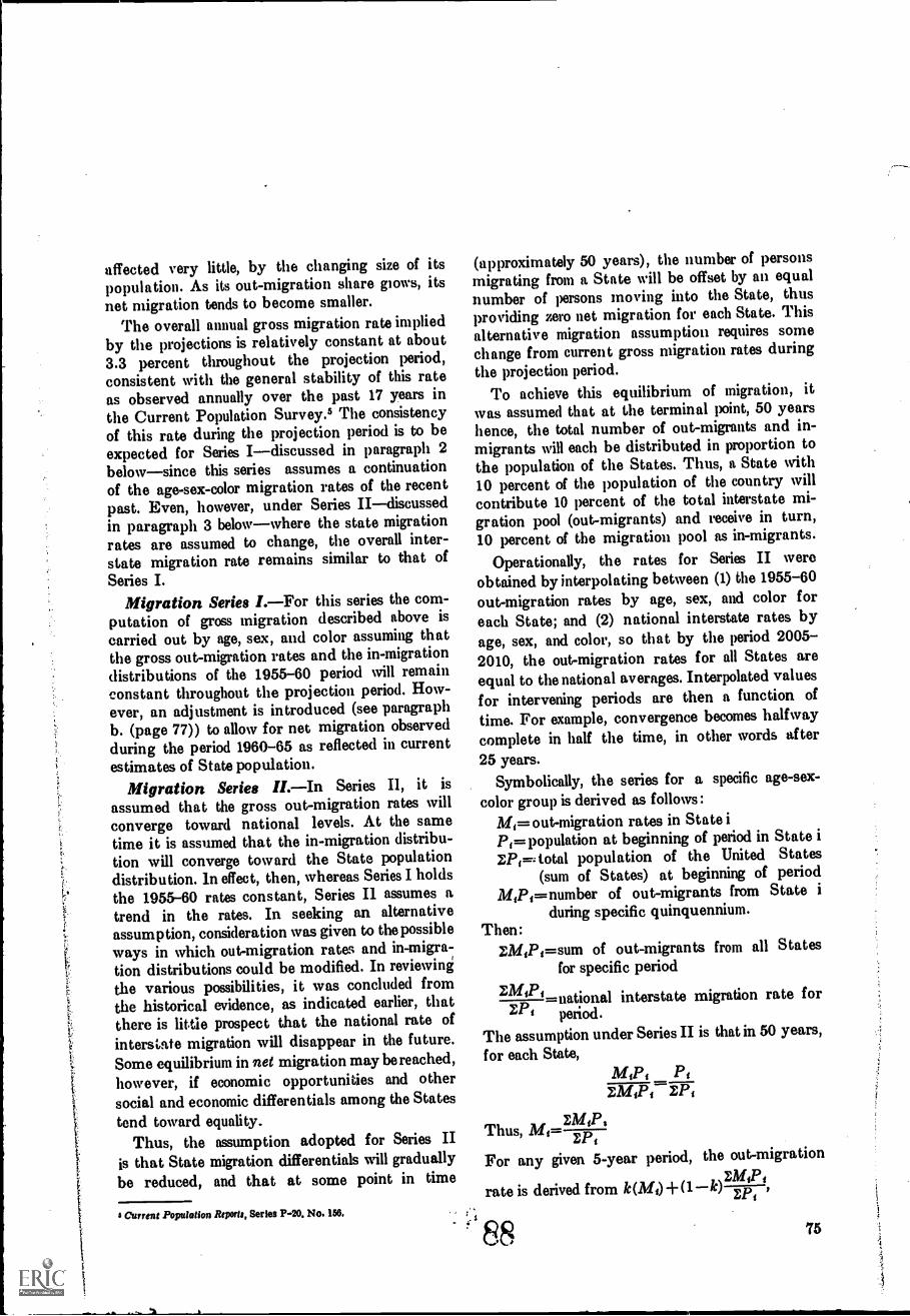
affected very little, by the changing size of itspopulation. As its out-migration share glows, itsnet migration tends to become smaller.
'rhe overall annual gross migration rate impliedby the projections is relatively constant at about3.3 percent throughout the projection period,consistent with the general stability of this rateas observed annually over the past 17 years intbe Current Population Survey.s The consistencyof this rate during the projection period is to beexpected for Series Idiscussed in paragraph 2belowsince this series assumes a continuationof the age-sex-color migration rates of the recentpast. Even, however, under Series IIdiscussedin paragraph 3 belowwhere the state migrationrates are assumed to change, the overall inter-state migration rate remains similar to that ofSeries I.
Migration Series I.For this series the com-putation of gross migration described above iscarried out by age, sex, and color assuming thatthe gross out-migration rates and the in-migrationdistributions of the 1955-60 period will remainconstant throughout the projection period. How-ever, an adjustment is introduced (see paragraphb. (page 77)) to allow for net migration observedduring the period 1960-65 as reflected in currentestimates of State population.
Migration Series II.In Series II, it is
assumed that the gross out-migration rates will
converge toward national levels. At the sametime it is assumed that the in-migration distribu-tion will converge toward the State populationdistribution, ln effect, then, whereas Series I holdsthe 1955-60 rates constant, Series Il assumes atrend in the rates. In seeking an alternativeassumption, consideration was given to the possible
ways in which out-migration rates and in-migra-tion distributions could be modified. In reviewingthe various possibilities, it was concluded fromthe historical evidence, as indicated earlier, thatthere is little prospect that the national rate ofinterstate migration will disappear in the future.Some equilibrium in net migration maybe reached,
however, if economic opportunities and othersocial and economic differentials among the States
tend toward equality.Thus, the assumption adopted for Series II
is that State migration differentials will graduallybe reduced, and that at some point in time
Current Population Reports, Series P-20, No. 156.
(approximately 50 years), the number of personsmigrating from a State will be offset by an equalnumber of persons moving into the State, thusproviding zero net migration for each State. Thisalternative migration assumption requires somechange from current gross migration rates duringthe projection period.
To achieve this equilibrium of migration, itwas assumed that at the terminal point, 50 yearshence, the total number of out-migrants and in-migrants will each be distributed in proportion tothe population of the States. Thus, a State with10 percent of the population of the country willcontribute 10 percent of the total interstate mi-gration pool (out-migrants) and receive in turn,10 percent of tbe migration pool as in-migrants.
Operationally, the rates for Series II wereobtained by interpolating between (1) the 1955-60out-migration rates by age, sex, and color foreach State; and (2) national interstate rates byage, sex, and color, so that by the period 2005-2010, the out-migration rates for all States areequal to the national averages. Interpolated valuesfor intervening periods are then a function oftime. For example, convergence becomes halfwaycomplete in half the time, in other words after25 years.
Symbolically, the series for a specific age-sex-color group is derived as follows:
Mi.-out-migration rates in State ipopulation at beginning of period in State i
EP,=, total population of the United States(sum of States) at beginning of period
iliiPt=number of out-migrants from State iduring specific quinquennium.
Then:aliPt=sum of out-migrants from all States
for specific period
ZMiPtnational interstate migration rate forperiod.
The assumption under Series II is that in 50 years,for each State,
MA I)
Thus, .1111=EXP,EPtFor any given 5-year period,
rate is derived from k (M,) -I- (1
the out-migration
k)ZAZPi '
75
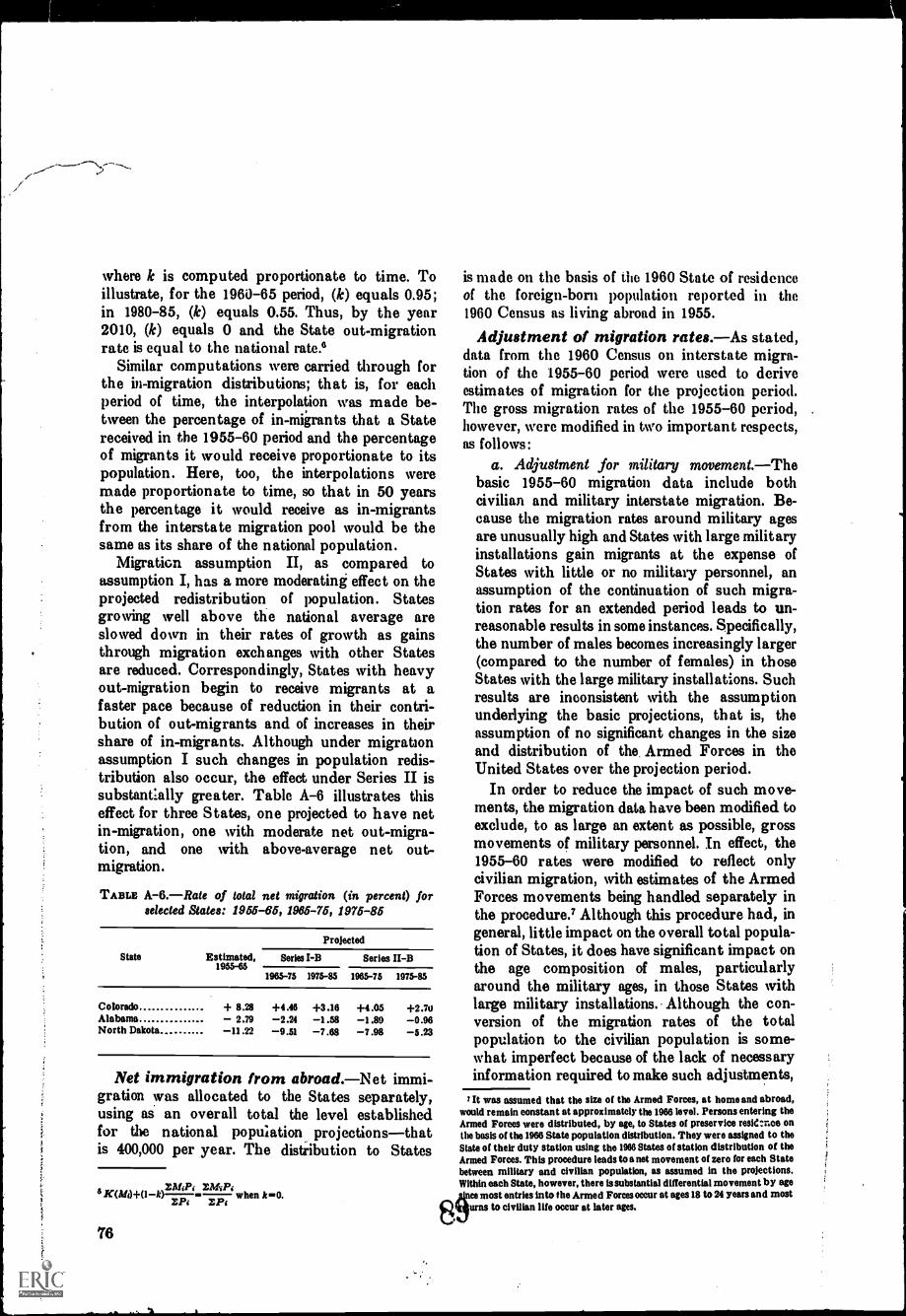
where k is computed proportionate to time. Toillustrate, for the 1960-65 period, (k) equals 0.95;in 1980-85, (k) equals 0.55. Thus, by the year2010, (k) equals 0 and the State out-migrationrate is equal to the national rate.°
Similar computations were carried through forthe in-migration distributions; that is, for eachperiod of time, the interpolation was made be-tween the percentage of in-migrants that a Statereceived in the 1955-60 period and the percentageof migrants it would receive proportionate to itspopulation. Here, too, the interpolations weremade proportionate to time, so that in 50 yearsthe percentage it would receive as in-migrantsfrom the interstate migration pool would be thesame as its share of the national population.
Migration assumption II, as compared toassumption I, has a more moderating effect on theprojected redistribution of population. Statesgrowing well above the national average areslowed down in their rates of growth as gainsthrough migration exchanges with other Statesare reduced. Correspondingly, States with heavyout-migration begin to receive migrants at afaster pace because of reduction in their contri-bution of out-migrants and of increases in theirshare of in-migrants. Although under migrationassumption I such changes in population redis-tribution also occur, the effect under Series II issubstantially greater. Table A-6 illustrates thiseffect for three States, one projected to have netin-migration, one with moderate net out-migra-tion, and one with above-average net out-migration.
TABLE A-6.Raie of total net migration (in percent) forselected States: 1955-65, 1985-75, 1975-85
State Estimated,1955-65
Projected
Series I-B Series II-B
1965-75 1975-85 1965-75 1975-85
Colorado + 8.28 +4 .46 +3.16 +4 .05 +2.70Alabama 2.79 2.24 1 .58 1 .89 0.96North Dakota 11 .22 9.51 7 .68 7 .98 5 .23
Net immigration from abroad.Net immi-gration was allocated to the States separately,using as an overall total the level establishedfor the national population projectionsthatis 400,000 per year. The distribution to States
Z2IfiPi6 IC(111)+(1k) when 1c=f1.P. Z.Pt
76
is made on the basis of the 1960 State of residenceof the foreign-born population reported in the1960 Census as living abroad in 1955.
Adjustment of migration rates.As stated,data from the 1960 Census on interstate migra-tion of the 1955-60 period were used to deriveestimates of migration for the projection period.The gross migration rates of the 1955-60 period,however, were modified in two important respects,as follows:
a. Adjustment for military movement.Thebasic 1955-60 migration data include bothcivilian and military interstate migration. Be-cause the migration rates around military agesare unusually high and States with large militaryinstallations gain migrants at the expense ofStates with little or no military personnel, anassumption of the continuation of such migra-tion rates for an extended period leads to un-reasonable results in some instances. Specifically,the number of males becomes increasingly larger(compared to the number of females) in thoseStates with the large military installations. Suchresults are inconsistent with the assumptionunderlying the basic projections, that is, theassumption of no significant changes in the sizeand distribution of the Armed Forces in theUnited States over the projection period.
In order to reduce the impact of such move-ments, the migration data have been modified toexclude, to as large an extent as possible, grossmovements of military personnel. In effect, the1955-60 rates were modified to reflect onlycivilian migration, with estimates of the ArmedForces movements being handled separately inthe procedure.7 Although this procedure had, ingeneral, little impact on the overall total popula-tion of States, it does have significant impact onthe age composition of males, particularlyaround the military ages, in those States withlarge military installations. Although the con-version of the migration rates of the totalpopulation to the civilian population is some-what imperfect because of the lack of necessaryinformation required to make such adjustments,
l It was assumed that the size of the Armed Forces, at home and abroad,would remain constant at approximately the 1966 level. Persons entering theArmed Forces were distributed, by age, to States of preservice resit:nce onthe basis of the 1966 State population distribution. They were assigned to theState of their duty station using the 1966 States of station distribution of theArmed Forces. This procedure leads to a net movement of zero for each Statebetween military and civilian population, as assumed in the projections.Within each State, however, there is substantial differential movement by age
8ce mostoteeintrilitaes ininto the Armat eladteForces occur at ages 18 to 24 years and most
urns
it is believed that the modification significantlyimproved the projections for those ages and
States where such adjustments were important.Because the age group 18 to 24 years is par-ticularly affected by this adjustment and be-cause migration rates are very high for thisgroup, the projected values should be inter-preted with caution.
b. Adjustments for net migration, 1960 to1965.It was also necessary to adjust the 1955-60 rates in order to take account of populationchanges, mainly due to net migration, that haveoccurred since 1960. The resulting adjustmentapplies with equal effect to both migrationSeries I and II. The latest current populationestimates, by age available at the time theseprojections were undertaken were those for 1965published in report No. 354 of this series. Esti-mates of net migration by age consistent withthe 1965 population estimates were developed
for the period 1960-65. The 1955-60 grossmigration rates were adjusted in such a mannerthat, when used for the period 1960-65, theyproduced estimates of net migration by agefor each State about the same as that derivedfrom the independent current estimates.
The adjustment was accomplished by firstcomputing "projections" of net interstate mi-gration for the 1960-65 period using the 1955-60migration rates and then comparing theseestimates with the independent current estimatesfor the 1960-65 period. The difference betweenthe initial "projections" of net migration for1960-65 for each State, and the net migrationdeveloped consistent with the current estimatesfor 1960-65 was then used to adjust the 1955-60out-migration rates and the distribution ofin-migrants. The amount of adjustment as-signed to each flow, for each age-sex-colorgroup, was determined by the ratios of grossout-migrants and gross in-migrants, respec-tively, to their sum. A second computationbeginning with April 1, 1960, using the 1955-60
rates as adjusted, now yielded figures whichclosely approximated the 1965 independentcurrent es timates.
Part of the adjustment was retained duringthe projection period, thus assigning weightto the 1960-65 migration experience in thesubsequent derivation of the projections. From1965 to 1970, three-quarters of the adjustmentwas used; from 1970 to 1975, one-half; and forthe period 1975-80, one-quarter. From 1980
to 1985, the original 1955-60 values wereemployed. In effect, then, for the bulk of theprojection period, the migration assumptionsrepresent a blending of the 1955-60 grossmigration experience with the more recent1960-65 net migration estimates. This pro-cedure yields projections which can be generallydescribed as "based on the assumption thatrecent migration rates would prevail during theprojection period." This system of combiningthe migration experience of the two most recentperiods recognizes, and takes advantage of, thelarge amount of detailed data available fromthe census for the 1955-60 period, whilebroadening the base period of the migrationprojections.
Other Series Developed by the U.S. Bureau of theCensus
The projections described above result in fourmain seriesthat is, two assumptions concerning
future interstate migration combined with twolevels of fertility (labelled Series I-B, I-D, II-B,and II-D). A number of other series based onalternative interstate migration assumptions weredeveloped to provide background data for select-ing the projection series to be used for specificprojects.
One alternative series, designated as SeriesIII, assumes "no net migration" for each Stateduring the projection period. In this series, ithas been assumed that, regardless of grosspopulation movement, net interstate migrationfor each State in each period after 1965 willbalance out. to zero (for each age-sex-color groupas well as for the total). This series is usefulfor measuring the impact on the populationprojections of alternative assumptions of futureinterstate migration. Net immigration fiom abroadat the rate of 400,000 per year is assumed tocontinue for this series.
Another alternative set of projections affectsonly the nonwhite population in States. Generallyspeaking, the rates and pattern of nonwhitemigration differ to an appreciable degree fromthose of the white population. This alternativeprojection series has been derived to illustratethe effect of interstate migration on the popu-lation distribution of the nonwhite population ifinterstate migration rates for whites and non-whites should become equal. For this series,
it was assumed that for each State, the non-white out-migration rates of the 1955-60 period
90
77
will converge toward those of the white popula-tion, so that 50 years hence, the out-migratiorates of the nonwhites, State by State, wouldequal to those of the whites. It was furtherassumed that the distribution by State of desti-nation would, in 30 ycars, also be the same asfor the white population.
A special set of projections was also derivedfor the District of Columbia. The District ofColumbia is a small area and exclusively urban.Its population composition, the city's position asthe core of a large metropolitan area, and pastsuburbanization, which has involved substantialinterstate movement, all contribute to unusualgross interstate migration patterns. Further-more, it is quite possible, because of present andplanned land use, that the current populationis not very far below the practical maximum.Consequently, migration assumptions 1 and IImay not be at all appropriate for this area.
School Enrollment Projections8The projections of school enrollment were made
by the participation rate method. Projectionswere made of enrollment rates by age and sex,and these rates were applied to the projections oftotal population to obtain the number enrolled.Four series are shown, designated as B-1, B-2,D-1, and D-2. The two series designated as "B"are consistent with the series of populationprojections designated as "B" series. Hence theseprojections imply a moderate rise in fertility. Thetwo series designated as "D" are consistent withthe projections designated as "D" series. Theyimply a sharp drop in fertility.
'Source: U.S. Bureau of the Census. Population Estimates. "Summaryof Demographic Projections," Series P-25, No. 388, March 14, 1968, pp.26-27.
78
The two series designated as "1" imply markedincreases in the percent of the population en-rolled in school at the older ages. The two seriesdesignated as "2" imply that the increase atthese ages will be less rapid. There is little differ-ence between the two assumptions at the youngerages, for enrollment is already near 100 percent.There are important differences at the older ages,however.
Actually, it was the age-specific rates for thosenot enrolled in school which were projected.Series 1 assumes that the decline in the "non-enrollment rates" will continue at the annualrate observed for the period of 1950-1952 to1963-1965. The complements of these rates arethe enrollment rates. The Series 2 enrollmentrates are the average of the Series 1 rates and therates achieved in 1965. They imply that the in-crease in enrollment will be half that assumed forSeries 1. The projections distribute enrollmentamong three levels of school: elementary (in-cluding (kindergarten), high school, and college andprofessional school. This step was also made bythe participation rate method. Projections weremade of the percentage distribution among thethree levels of school for each age-sex group, andthese percentages were applied to the projectionsof the enrolled population by age and sex. Series 1implies that the proportion of enrollment at agiven level of school would shift between 1964and 1990 by the same overall percent as between1951 and 1964. In effect, since the projectionperiod was twice as long as the base period, theproportions were assumed to change about one-half as rapidly in the future as in the,recent past.The series 2 proportions are the average of theSeries 1 proportions and the proportions in 1965.
APPENDIX B
SMOOTHING AGE DISTRIBUTIONS '
Definitions, Usages and LimitationsOne method often used consists of applying sets
of constant multipliers to the enumerated 5-yearage groups in order to obtain a smoothed distri-bution by single years of age. These multipliersalso are of special interest, for making populationestimates when the census does not present databy single years of age. There are many differentkinds of interpolation proceduresthat is, inter-polating within a 5-year age group so as to obtainestimates for single years; the procedure presentedbelow is often used by the U.S. Bureau of tbeCensus. These constant multipliers, or weights,are based on Sprague's osculatory fifth differenceformula.2 Another set of weights, somewhatsimilar to those derived from the Sprague formula,is that of Beers.'
The Sprague multipliers smooth (or graduate)the data reported into halves, fifths, or tenths. A10-year period can be divided into single years ortwo 5-year periods; for example, a 2-year periodcan be divided into single years; a 5-year periodcan be divided into single years; and so forth. Inthe following paragraphs we show the detailedprocedures for using the fifths; brief comments onthe use of the halves and tenths follow.
The Sprague MultipliersDividing into Fifths
The Sprague fifths multipliers simply redistrib-ute the number within the 5-year age period intoestimated numbers for single years of age, withoutin any way altering the total reported for the 5-year age period. Thus in applying it, the data arefirst compiled into 5-year age periods; original
Taken in part from Handbook of Statistical Methods for Demographers, byA. J..Taffe, U.S. B ureau of the Census, Washington, D.C., third printing, 1960,pp. 94-100.
2 For a derivation of Sprague's formula, see T. W. Clover, United States LifeTables, U.S. Bureau of the Census, Washington, 1931, pp. 344 and 345.
3 Henry S. Beers, "Modified-Interpolation Formulas that Minimize FourthDifferences," The Record, American Institute of Actuaries, Vol. XXXIV,Part I, No. 69, June 1045, pp. 14-20. NOTE. Table numbers ours.
tabulations by single years of age are not used.The same procedures, with but very little modifi-cation, can be used to smooth sets of rates by age,as for example, the proportion of the populationof single marital status by 1-year age periods;also, age-specific birth raieti for women by singleyears of age can be estimated from data on ratesfor 5-year age groups.
The limitations of this method are as follows:If any particular 5-year age group is greatly inerror due to under-/or over-enumeration, thismethod will not correct such deficiencies; theymust be corrected by graphic interpolation or bycalculating the expected number of survivors fromthe preceding census.
If the original data curve very rapidly fromone single year to the next, as is the case with theproportion of single marital status during theteen ages, this formula is somewhat inadequate.In such cases graphic smoothing may be the best.Thus, for example, in smoothing the proportionsingle for each year of age from age 15 to age 100,it may be best to use graphic smoothing for theage group 15 to 19 and for the older age groups.The specific older ones to which it should beapplied will depend on how "regular" or "irregu-lar" the data appear; this "irregularity" may rep-resent respondents' biases which should besmoothed out by actually altering the reportednumbers or percentages for given 5-year agegroups. For all intermediate 5-year age groupsthe formula should be adequate.
This formula may also be inadequate for thevery youngest age groupsunder 5, and 5 to 9years old. If birth and death statistics are avail-able, it is preferable to calculate these ages bysingle years on the basis of the vital statistics.Only if complete and accurate birth and deathstatistics are not available, should these smooth-ing procedures be applied to the 5-year groupsas enumerated by the census.
:
79
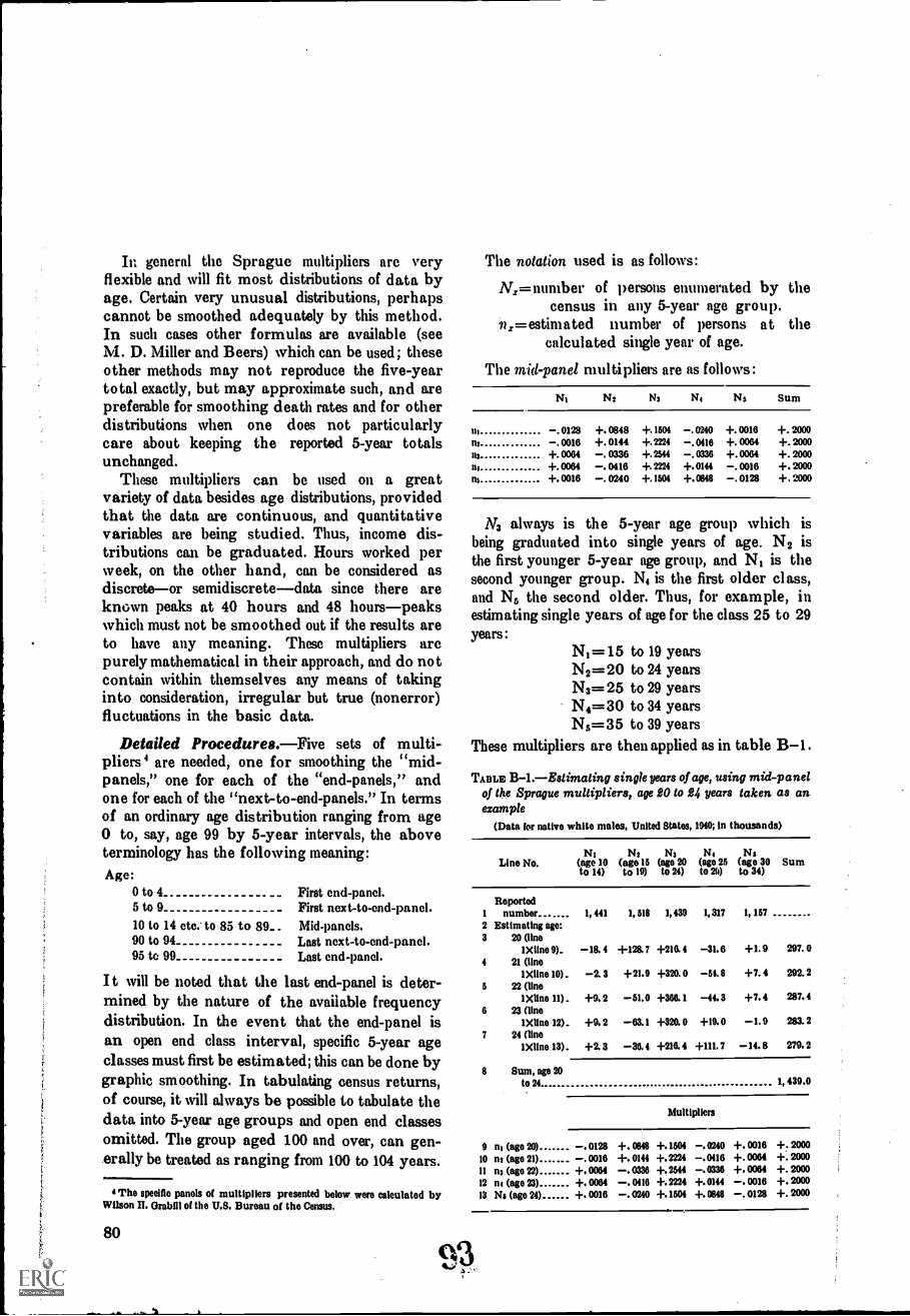
In general the Sprague multipliers are veryflexible and will fit most distributions of data byage. Certain very unusual distributions, perhapscannot be smoothed adequately by this method.In such cases other formulas are available (seeM. D. Miller and Beers) which can be used; theseother methods may not reproduce the five-yeartotal exactly, but may approximate such, and arepreferable for smoothing death rates and for otherdistributions when one does not particularlycare about keeping the reported 5-year totalsunchanged.
These multipliers can be used on a greatvariety of data besides age distributions, providedthat the data are continuous, and quantitativevariables are being studied. Thus, income dis-tributions can be graduated. Hours worked perweek, on the other hand, can be considered asdiscrete-or semidiscrete-data since there areknown peaks at 40 hours and 48 hours-peakswhich must not be smoothed out if the results areto have any meaning. These multipliers arepurely mathematical in their approach, and do notcontain within themselves any means of takinginto consideration, irregular but true (nonerror)fluctuations in the basic data.
Detailed Procedures.-Five sets of multi-pliers4 are needed, one for smoothing the "mid-panels," one for each of the "end-panels," andone for each of the "next-to-end-panels." In termsof an ordinary age distribution ranging from age0 to, say, age 99 by 5-year intervals, the aboveterminology has the following meaning:Age:
0 to 4 First end-panel.5 to 9 First next-to-end-panel.10 to 14 etc. to 85 to 89 Mid-panels.90 to 94 Last next-to-end-panel.95 to 99 Last end-panel.
It will be noted that the last end-panel is deter-mined by the nature of the available frequencydistribution. In the event that the end-panel isan open end class interval, specific 5-year ageclasses must first be estimated; this can be done bygraphic smoothing. In tabulating census returns,of course, it will always be possible to tabulate thedata into 5-year age groups and open end classesomitted. The group aged 100 and over, can gen-erally be treated as ranging from 100 to 104 years.
4 The specific panels of multipliers presented below were calculated byWilson II. Grabill of the U.S. Bureau of the Census.
80
The notation used is as follows:
N.r= number of persons enumerated by thecensus in any 5-year age group.
kr=estimated number of persons at thecalculated single year of age.
The mid-panel multipliers are as follows:
N1 N2 N3 N4 N3 sum
Ui -.0128 +. 0848 +.1504 -. 0240 +. 0016 +. 2000-. 0016 +.0144 +.2224 -.0416 +. 0004 +. 2000
as +. 0064 -. 0336 +.2544 -.0336 +. 0064 +. 2000st,
ns
+.0064+. 0016
-. 0416-. 0240
+.2224+.1504
+.0144+.0848
-. 0016-.0128
+. 2000+. 2000
N3 always is the 5-year age group which isbeing graduated into single years of age. N2 isthe first younger 5-year age group, and N, is thesecond younger group. N4 is the first older class,and NG the second older. Thus, for example, inestimating single years of age for the class 25 to 29years:
N1=15 to 19 yearsN2=20 to 24 yearsN3= 25 to 29 yearsN4= 30 to 34 yearsNG=35 to 39 years
These multipliers are then applied as in table B-1.
TABLE B-1.-Estimating single years of age, using mid-panelof the Sprague multipliers, age 20 to 24 years taken as anexample
(Data for native white males, United States, 1940; In thousands)
Line No.N3 NI N3 N4 Ns
(age 10 (age Is (age 20 (age 25 (age 30 Sumto 14) to 19) to 24) to 20) to 34)
Reported1 number2 Estimating age:3 20 (line
1Xline 9).4 21 (line
1 Xline 10)6 22 (line
1Xline 11)6 23 (lino
1Xline 12).7 24 (lino
1Xline 13).
1, 441 1, 618 1,439 1,317 1, 157
-18. 4 +128.7 +216.4 -31.6 +1.9 297. 0
-2. 3 +21.9 +320. 0 -M. 8 +7. 4 292. 2
+9.2 -51.0 +366.1 -44.3 +7.4 287.4
+9. 2 -63.1 +3211 0 +19. 0 -1. 9 283. 2
+2. 3 -35. 4 +216.4 +111. 7 -14. 8 279. 2
8 Sum, ago 20to 24 1, 439.0
9 nl (age 20)10 ns (age 21)11 ns (age 22)12 n4 (ago 23)13 Ns (ago 24)
Multipliers
-.0128 +. 0848 +.1504 -.0240 +. 0016 +. 2000
- 0016 +. 0144 +.2224 -.0416 +. 0064 +. 2000+.0064 -. 0336 +.2544 -.0336 +. 0064 +. 2000
+. 0064 -. 0416 +.2224 +.0144 -. 0016 +. 2000
+. 0016 -. 0240 +.1504 +. 0848 -. 0128 +. 2000
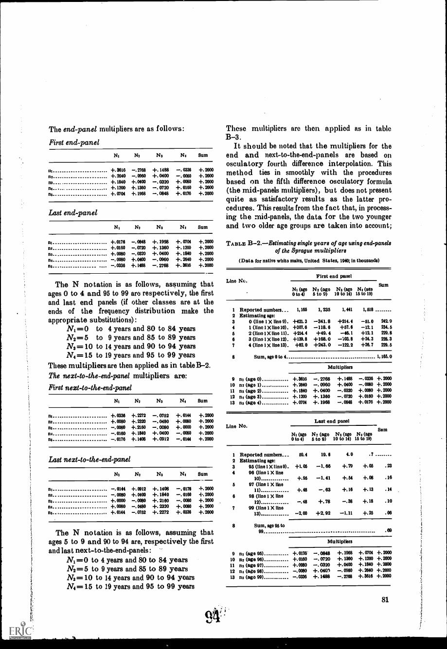
The end-panel multipliers are as follows:
First end-panel
Nr N3 Ni Sum
ttinsm.nitts
+.3616+.2640+. 1840+.1200+. 0704
-.2768-.0960+.0400+.1360+. 1968
+. 1488+. 0400
0320-. 0720-. 0848
-. 0336-. 0080+- 0°60+. 0160+. 0176
+. 2000+. 2000
+. 2°°°+.2000+. 2000
Last end-panel
NI Nr N3 Ni Sum
+.0176 -.0848 +. 1958 +. 0704 +.2000ni +.0160 -.0720 +. 1360 +. 1200 +. 2000
+.0080 -.0320 +. 0400 +. 1840 +. 2000
na - 0080 +.0100 -. 0960 +. 2640 +.2000ns - 0336 +.1488 -.2768 +. 3616 +.2000
The N notation is as follows, assuming thatages 0 to 4 and 95 to 99 are respectively, the firstand last end panels (if other classes are at theends of the frequency distribution make theappropriate substitutions):
N1=0 to 4 years and 80 to 84 yearsN2=5 to 9 years and 85 to 89 yearsN3 = 10 to 14 years and 90 to 94 yearsN4=15 to 19 years and 95 to 99 years
These multipliers are then applied as in table B-2.The next-to-the-end-panel multipliers are:
First next-to-the-end-panel
NI Nt N3 NI Sum
+.0336 +.2272 -. 0752 +. 0144 -I-. 2000
nt +.0080 +.2320 -.0480 +.0080 -I-. 2000
tts - 0080 +.2160 -. 0080 +. 0000 +. 2000
na +.1840 +. 0400 -. 0080 2000
ns -.0176 -I-. 1408 +. 0912 -. 0144 +. 2000
Last next-to-the-end-panel
NI Nr N3 NI Sum
nl - 0144 +.0912 +. 1408 -.0176 2000
nt._ - 0080 +.0400 +. 1840 -.0160 2000
+.0000 -. 0080 +. 2160 -. 0060 2000
+.0080 -.0480 +. 2320 +.0080 20004-. 0144 -.0752 +. 2272 +. 0336 +.2000
The N notation is as follows, assuming that,ages 5 to 9 and 90 to 94 are, respectively the firstand last next-to-the-end-panels:
N1=0 to 4 years and 80 to 84 yearsN2=5 to 9 years and 85 to 89 yearsN3 =10 to 14 years and 90 to 94 yoarsN4= 15 to 19 years and 95 to 99 years
These multipliers are then applied as in tableB-3.
It should be noted that the multipliers for theend and next-to-the-end-panels are based onosculatory fourth difference interpolation. Thismethod ties in smoothly with the proceduresbased on the fifth difference osculatory formula(the mid-panels multipliers), but does not presentquite as satisfactory results as the latter pro-cedures. This results from the f act that, in process-ing the mid-panels, the data for the two youngerand two older age groups are taken into account;
TABLE B-2.-Estimaling single years of age using end-panelsof the Sprague multipliers
(Data for native white males, United States, 1940; in thousands)
Lino N.
1 Reported numbers...2 Estimating age:3 0 (line 1 X lino 9).4 1 (line 1 X lino 10).5 2 (lino 1 X lino 11).6 3 (line 1 X line 12).7 4 (lino 1 X line 13).
Sum, ago 0 to 4
9 ni (age 0)10 ns (ago 1)11 ns (age 2)12 ni (age 3)13 ns (age 4)
First end panel
NI (ago0 to 4)
N2 (ago5 to 9)
N3 (age10 to 14)
Na (ago15 to 19)
Sum
1,165 1, 235 1,441 1,518
+421.3 -341.8 +214.4 -51.0 242.9+307.6 -118.6 +57.6 -12.1 234.5+214.4 +49. 4 -46.1 +12.1 229.8+139.8 +168.0 -103.8 +24. 3 228.3+82. 0 +243. 0 -122.2 +26.7 229.5
1,165.0
Multipliers
+.3616 -.2768 +.1488 -.0336 +.2000+.2640 -. 0960 +.0100 -.0080 +.2000+.1840 +.0900 -.0320 +.0080 +.2000+.1200 +. 1360 -.0720 +.0160 +.2000+.0701 +. 1968 -.0848 +.0176 +.2000
Line No.
1 Reported numbers...2 Estimating age:3 95 (line 1 X lino9)4 96 (line 1 X line
10)5 97 (line 1 X lino
11)6 98 (lino 1 X lino
12)7 99 (line 1 X lino
13)
8 Sum, age 95 to99_
9 nl (age 95)10 ns (age 96)11 rir (agO 97)12 ni (age N)13 ns (ago 99)
Last end panel
NI (age0 to 4)
N2 (age5 to 9)
N3 (age Na (age10 to 14) 15 to 19)
Sum
59.4 19.6 4.0 .7
+1.05 -1.86 +.79 +.05 .23
+.95 -1.41 +.54 +.06 .16
+.48 -.63 +.16 +.13 .14
-.48 +.78 -.38 +.18 .10
-2.00 +2.92 -1.11 +.25 .06
69
Multipliers
+.0176* -. 0848 +. 1968 +. 0704 +. 2000+.0160 -. 0720 1360 +. 1200 4-.2000+.0080 -.0320 +.0100 +.1840 +.2000-. 0080 4-. 0901 -. 0960 +. 2640 +.2000-.0336 4-. 1488 -. 2768 +.3616 +. 2000
81
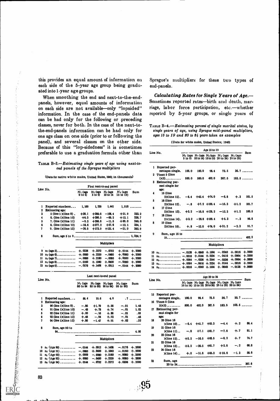
this provides an equal amount of information oneach side of the 5-year age group being gradu-ated into 1-year age groups.
When smoothing the end and next-to-the-end-panels, however, equal amounts of informationon each side are not available-only "lopsided"information. In the case of the end-panels datacan be had only for the following or precedingclasses, never for both. In the case of the next-to-the-end-panels information can be had only forone age class on one side (prior to or following thepanel), and several classes on the other side.Because of this "lop-sidedness" it is sometimespreferable to use a graduation formula other than
TABLE B-3.-Estimaling single years of age using next-to-end panels of the Sprague multipliers
(Data for native white males, United States, 1940; In thousands)
Line No.First next-to end panel
NI (age NI (age 113 (age N4 (age Sum0 to 4) 5 to 9) 10 to 14 15 to 19)
1 Reported numbers._2 Estimating age:3 5 (line 1 )(line 9) .4 6. (line 1Xline 10)5 7. (line 1Xline 11)6 8. (line 1Xline 12)7 9. (lino 1Xline 13)
8 Sum, ago 5 to 9
9 m (age 5)10 n2 (age 6)11 n: (age 7)12 n4 (age 8)13 ns (age 9)
Line No.
1,165 1, 235 1,441 1, 518
+39.1 +280.6 -108.4 +21. 9 233.2+9.3 +286.5 -69.2 +12. 1 238.7-9.3 +266.8 -11.5 +00.0 246.0
-18.6 +277.2 +57.6 -12. 1 264.1-20.5 +173.9 +131.4 -21.9 262.9
1,234.9
Multipliers
+.0336 +.2272 4-.0752 +. 0144 +. 2000+.0080 +.2320 -.0480 +. 0080 +. 2000-.0080 +. 2160 -.0080 +. 0000 +. 2000-.0160 +. 1840 +.0400 -.0080 +. 2000-.0176 +.1408 +.0912 -.0144 +. 2000
1 Reported numbers2 Estimating age:3 90 (line 1Xline 9).4 91 (line lXlino 10)5 92 (line 1Xline 11)6 93 (line IXIIne 12)7 94 (line 1Xline 13)
Sum, age 90 to94
9 ns (Age 90)10 n: (Age 91)11 n: (Age 92)12 n4 (Age 93)13 ns (Age 94)
Last next-to-end panel
NI (age80 to 84
N: (age85 to 89)
N3 (age90 to 94)
N4 (ago95 to 99)
Sum
59. 4 19. 6 4. 0 . 7
-.86 +1.79 +.56 -.01 1.48-. 48 -I-. 78 +. 74 -. 01 1. 03+.00 -.16 +.86 -.01 .69+.48 -.94 +.93 -.01 .48+.86 -1.47 +.91 +.02 .32
4. 00
Multipliers
- 0144 +.0912 +.1408 -.0176 +.2000- 0080 +.0400 +.1840 -.0160 +. 2000+.0000 -. 0080 +.2160 -.0080 +. 2000+. 0080 -.0480 +.2320 +.0080 +. 2000+.0144 -.0752 +.2272 +. 0336 +.2000
82
Sprague's multipliers for these two types ofend-panels.
Calculating Rates for Single Years of Age.-Sometimes reported rates-birth and death, mar-riage, labor force participation, etc.-whetherreported by 5-year groups, or single years of
TABLE II-4.-Estimating percent of single marital status, bysingle years of age, using Sprague mid-panel multipliers,ages 15 to 19 and 20 to 24 years taken as examples
(Data for white males, United States; 1940)
Line No.Age 15 to 19
NI (age NI (age N3 (age NI (age Ns (age5 to 9) 10 to 14) 15 to 19) 20 to 24) 25 to 29)
Sum
I Reported per-centages single. 100. 0 100. 0 9& 4 73. 5 36. 7
2 Times 5 (lino1X5)
3 Estimating per-cent single forage:
4 15 (lino2X lino 11). -6. 4 +42.4 +74.0 -8. 8 +. 3 101. 5
5 16 (line2Xline 12). -.8 +7.2 +109.4 -15.3 +1.2 101.7
6 17 (lino2Xline 13). +3.2 -16.8 +125.2 -12. 3 +1.2 100.5
7 18 (lino2 XlIne 14). +3. 2 -20. 8 +109. 4 +5. 3 -. 3 96. 8
8 19 (lino2X line 15). +. 8 -12. 0 +74. 0 +31. 2 -2. 3 91. 7
500. 0 500. 0 492. 0 367. 5 183. 5
9 Sum, ago 15 to19 492.2
Multipliers
10 ns -.0128 +.0848 +.1504 -. 0240 +.0016 +.200011 n2 - 0016 +.0144 +.2224 -. 0410 +.0064 +.200012 n: +. 0064 -.0336 +.2544 -. 0330 0064 +.200013 n4 +.0064 -. 0416 +.2224 +. 0144 -.0016 +.200014 ns +.0016 -.0240 +.1504 +. 0848 -.0128 +.2000
Line No.Age 20 to 24
NI (age N: (age N3 OP NI (ago Ns (age10 to 14) 15 to 19) 20 to24) 25 to 29) 30 to 34)
Sum
15 Reported per-centages single. 100.0 98.4 73.5 36. 7 20. 7
16 Times 5 (line15)(5)
17 Estimating per-cent single torage:
18 20 (lino 16X Une 10) -6. 4 +41. 7 +55. 3 -4. 4 +. 2 86. 4
19 21 (line 16Xline 11) -.8 +7.1 +81.7 -7. 6 +.7 81.1
20 22 (line 16X line 12) __ +3. 2 -16. 5 +93.5 -IL 2 +. 7 74. 7
21 23 (line 16X line 13) - - +3. 2 -20. 5 +81. 7 +2. 6 -. 2 66.8
22 24 (lino 16X lino 14)._ +.8 -11.8 +55.3 +15.6 -1. 3 58.0
500. 0 492. 0 367. 5 183. 5 103. 5
23 Sum, ago20 to 24 367.6
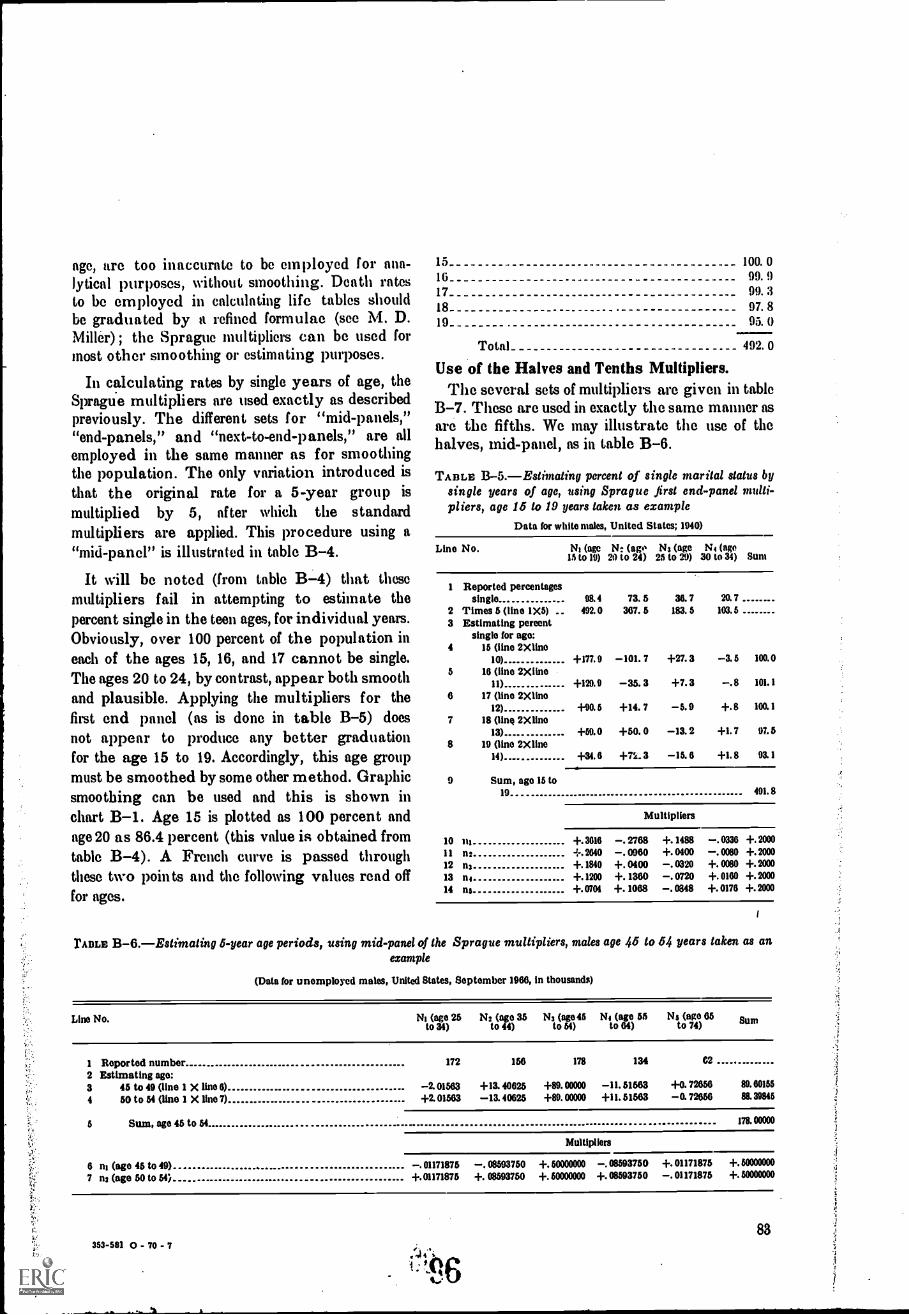
age, are too inaccurate to be employed for ana-lytical purposes, without smoothing. Death ratesto be employed in calculating life tables shouldbe graduated by a refined formulae (see M. D.Miller) ; the Sprague multipliers can be used formost other smoothing or estimating purposes.
In calculating rates by single years of age, theSprague multipliers are used exactly as describedpreviously. The different sets for "mid-panels,"tt end-panels," and "next-to-end-panels," are allemployed in the same manner as for smoothingthe population. The only variation introduced isthat the original rate for a 5-year group ismultiplied by 5, after which the standardmultipliers are applied. This procedure using a"mid-panel" is illustrated in table B-4.
It will be noted (from table B-4) that thesemultipliers fail in attempting to estimate thepercent single in the teen ages, for individual years.Obviously, over 100 percent of the population ineach of the ages 15, 16, and 17 cannot be single.The ages 20 to 24, by contrast, appear both smoothand plausible. Applying the multipliers for thefirst end panel (as is done in table B-5) doesnot appear to produce any better graduationfor the age 15 to 19. Accordingly, this age groupmust be smoothed by some other method. Graphicsmoothing can be used and this is shown inchart B-1. Age 15 is plotted as 100 percent andage 20 as 86.4 percent (this value is obtained fromtable B-4). A French curve is passed throughthese two points and the following values read offfor ages.
15 100. 016 99. 917 99. 318 97. 819 95. ()
Total 992. 0
Use of the Halves and Tenths Multipliers.The several sets of multipliers are given in table
B-7. These are used in exactly the same manner asare the fifths. We may illustrate the use of thehalves, mid-panel, as in table B-6.
TABLE B-5.-Estimating percent of single marital status bysingle years of age, using Sprague first end-panel multi-pliers, age 15 to 19 years taken as example
Data for white males, United States; 1940)
Lino No. N: (age15 to 19)
N: (ago2) to 24)
N3 (age25 to 29)
N4 (age30 to 34) Sum
1 Reported percentagessingle 98.4 73. 5 36. 7 20. 7
2 Times 5 (line 1X5) 492. 0 367. 5 183. 5 103. 5
3 Estimating percentsingle for ago:
4 15 (ine 2Xlino10) +177.9 -101. 7 +27.3 -3.5 100.0
5 16 (One 2XiinoII) +129.9 -35.3 +7.3 -.8 101.1
6 17 (IMe 2Xline12) +90.5 +14. 7 -5.9 +.8 100.1
7 18 (lin@ 2Xline13) +59.0 +50. 0 -13.2 +1.7 97.5
8 19 (line 2Xline14) +34.6 +rt. 3 -15. 6 +I. 8 93.1
9 Sum, age /5 to19 491. 8
Multipliers
10 ni +.3010 -.2788 +.1488 -.0336 +.200011 n2 + 2040 -.0960 +.0400 -.0080 +.200012 n3 +.1840 +. 0400 -.0320 +.0080 +.200013 n, +.1200 +. 1360 -.0720 +.0160 +.200014 ns +.0701 +. 1068 -.0848 +.0176 +.2000
rABLE B-6.-Estimating 6-year age periods, using mid-panel of the Sprague multipliers, males age 45 to 54 years taken as anexample
(Data for unemployed males, United States, September 1966, in thousands)
Lino No. NI (ago 25to 34)
N2 (age 35to 44)
N3 (ago 45to 54)
NI (age 55to 64)
Ns (age 65to 74) Sum
1
2Reported numberEstlmating age:
172... 156 178 134 C2
3 45 to 49 (line 1 X lino 6) -2. 01563 +13. 40625 +89. 00000 -II. 51563 +0. 72656 SI 00155
4 50 to 54 (line 1 X line 7) +2. 01563 -13. 40625 +89. 00000 +II. 51563 -0. 72656 88. 39845
5 Sum, age 45 to 54 178.00000
Multipliers
ni (ago 45 to 49) -.01171875 -. 08593750 +.60000000 -. 08593750 +.01171875 +.50000000
7 n2 (age 50 to 54) +.01171875 +. 08593750 +.60000000 +.08593750 -.01171875 +.M000000
353-501 0 - 70 - 7
qlg83
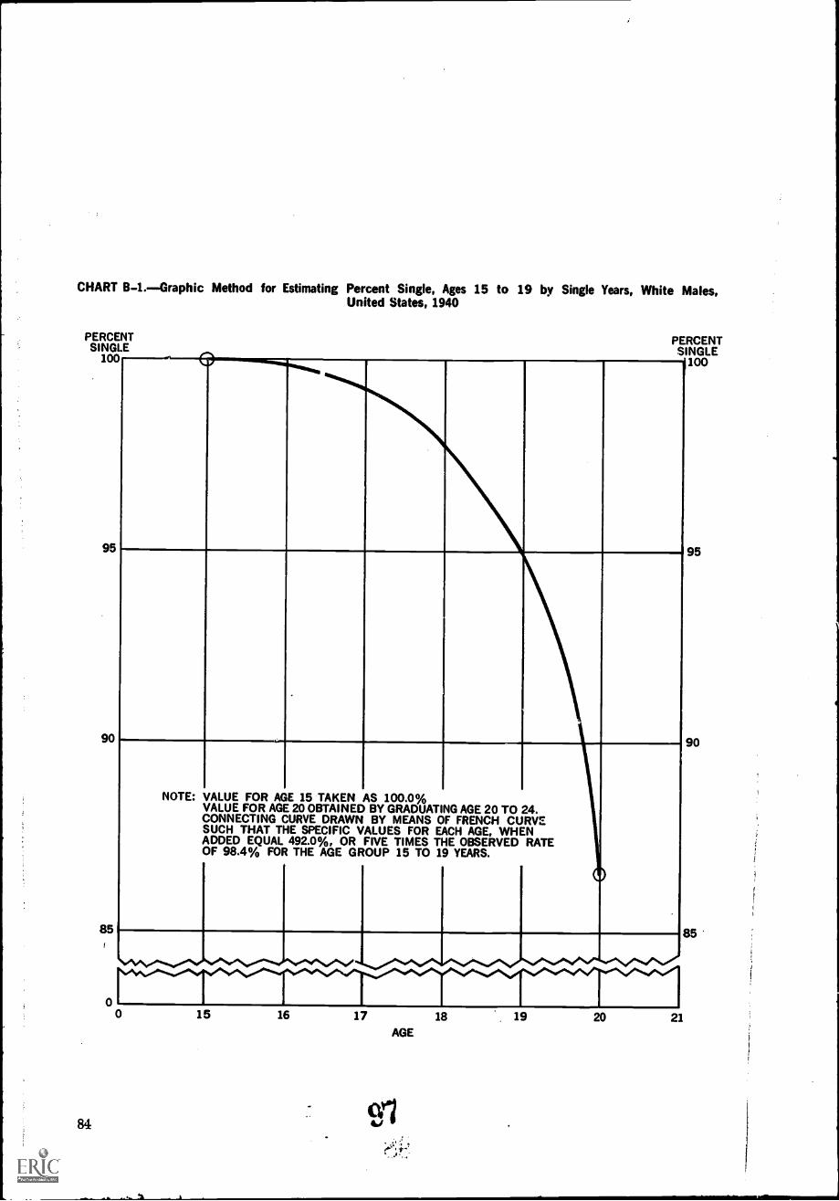
CHART B-1.Graphic Method for Estimating Percent Single, Ages 15 to 19 by Single Years, White Males,United States, 1940
PERCENTSINGLE
100
95
90
85
0
84
PERCENTSINGLE4100
NOTE: VALUE FOR AGE 15 TAKEN AS 100.0%VALUE FOR AGE 20 OBTAINED BY GRADUATING AGE 20 TO 24.CONNECTING CURVE DRAWN BY MEANS OF FRENCH CURVESUCH THAT THE SPECIFIC VALUES FOR EACH AGE, WHENADDED EQUAL 492.0%, OR FIVE TIMES THE OBSERVED RATEOF 98.4% FOR THE AGE GROUP 15 TO 19 YEARS.
0 15 16 17AGE
(s1
18 19 20
95
90
85
21
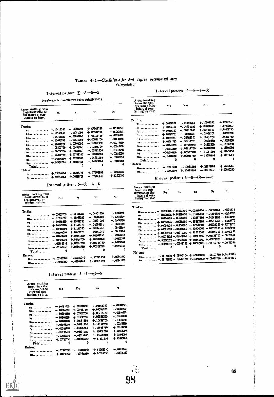
TABLE B-7.-Coefficients for 3rd degree polynomial areainterpolation
Interval pattern: C)-5-5-5 Interval pattern: 5-5-5-10
(No always is (ho category beingsubdivided) Areas resultingfrom the sub-division of theinterval con-
tinning No into:
N-3 N-3 N-1 No
Areas resulting fromthe subdivision of Nsthe interval con-taining No into:
.1,13 N2 N3
Tenths:
Tenths:nl +.00866250 -. 01248750 +. 10398750 +.02983750
m +. 19916250 -.18398750 +.09048750 -.02060250 n2 -I-. 00893750 -.04231250 +.09281250 +.01056250
n2 +.16743750 -.11281250 +.06831250 -.01293750 113 -L. 00850250 -. 03918750 +.07768750 +.05293750
m.. +.14308250 -.06768750 +.03118750 -. 00656250 no +. 00743750 -.03281250 +.05831250 +.06706250
118 +.12093750 -.02831250 +.00881250 -.00143750 ns +.00546250 -. 02788750 +. 03938750 -3-. 08303750
in -I-. 1009e250 +.00501250 - 00911250 +.00253750 ns +.00253250 -.00911250 +.00561250 +.10096250
na +.08303750 +.03438750 - 02288750 -1-.00548250 112 -.00143750 +.00881250 -.02831250 +.12093750
117.. +.06706250 +.05831260 - 03281250 +.00793750 nt -... 00056250 -F. 03118750 -.06768750 +.14300250
no +.05293750 +.07788750 - 03918750 +.00856250 nt -.01203750 +.05831250 .--. 11281250 -F.16743750
nt.. +.04056250 +.09281250 - 04231250 +.00893750 mo -.02066250 +.09048750 -.16398750 +.19416250
n N. 1-. 02063750 -3-. 10308750 - 04248750 +.00866250 Total 0 o o 1
Total 1 o o 0 Halves:
Halves:nl +.03900250 -. 17968750 +.36718750 +.27343750
m +.72658250 -.38718750 +. 17060750 -.03906250 m -.03906250 +. 17968750 -.36718750 +.72658250
m +.27343750 +.36718750 -. 17968750 +.03900250 Interval pattern: 5-5-0-5-5Interval pattern: 5-00--5-5
Areas resultingfrom the sub-division of the
interval con-taining No into:
N-1 N.-1 No NI No
Areas resulting fromthe subdivision of N-Ithe interval con-taining No into:
No Ng N3
Tenths:Tenths:
m +.02006250 +.11151250 -.04001250 +.00783750 m -.00759375 +.05103750 +.06595000 -.00963750 +.00024375
113 +.01203750 -F.11568750 -.03518750 +.00656250 22. -.00520625 +.03376250 +.08445000 -.01136250 +.00135625
n2 +.00656250 +.11681250 -.02831250 +.00493750 223 - 00220625 +.01538750 +.10357500 -.01948750 +.00273125
214.. +.00143750 +.11518750 -.0106870 +.00306250n8 +.00060625 -.00098750 +.11882500 -.02211250 +.00366875
in -.00753750 -F.11111250 -.00961250 +.001037as ns +.00268125 -.01328250 +.12720000 -.02033750 +.00371875
no - 00546250 -3-.10488750 +.00161250 -.00103750 ns -3-. 00371875 -.02033750 +.12720000 -.01326250 +.00268125
117 - 00743750 +.09881250 +.01368750 -.00306250 nr +.00366575 -.02211250 +.11882500 -.00098750 +.00060025
ns -.00858250 -1-.08718750 +.02631250 -.00493750 ns -3-. 00273125 -.01948750 -1-.10357500 +.01538750 -.00220625
no -.00893750 +.07831250 +.03918750 -.00650250 nt +.00135625 -.01938250 +.08445000 +.03376250 -.00520625
ma - 00360250 -1-.08448750 +. 05201250 -.00783750 no -3-. 00024375 -. 00963750 -I-. 06595000 +. 05103750 -.00759375
Total.... - . . o 1 o 0 Total 0 0 1 0 o
Halves:Halves:
nl +.03906250 +.57031250 -.13281250 +.02343750 n -.01171875 +.08593750 -3-.50000000 -.08593750 -1-.01171875
n2 -.03908250 +.42908750 -I-. 13281250 - 02343750 n2 -4-. 01171875 -.08593750 +.50000000 +.08593750 -.01171875
Interval pattern: 5-5-®-5
Areas resultingfrom the sub-division of theinterval con-
taining No into:
N.-2 N-I No NI
Tenths:in -.00783750 +.05201250 +.08448750 -.00886250
in -.00656250 +.03918750 +.07631250 -.00893750
112 - 00493750 +.02631250 +.08718750 -.00856250
-. 00306250 +.01368750 +.09681250 -.00743750
no -.00103750 +.00181250 -1-.10488750 -.00546250
+.00103750 -.00061250 +.11111250 -.00253750
ns +.00308250 -.01968750 -1-.11518750 +.00143750
no +.00493750 -.02831250 +.11681250 +.00056250
nt +.00656250 -.08518750 +. 11568750 +.01293750
me +.00783750 -.01001250 +.11151250 +.02086350
Total 0 0 1
Halves:in -.02343750 -4-. 13281250 +.42968750 -.03008250
nt -I-. 02343750 - -. 13281250 -I-. 57031250 -I-. 03906250
85
98
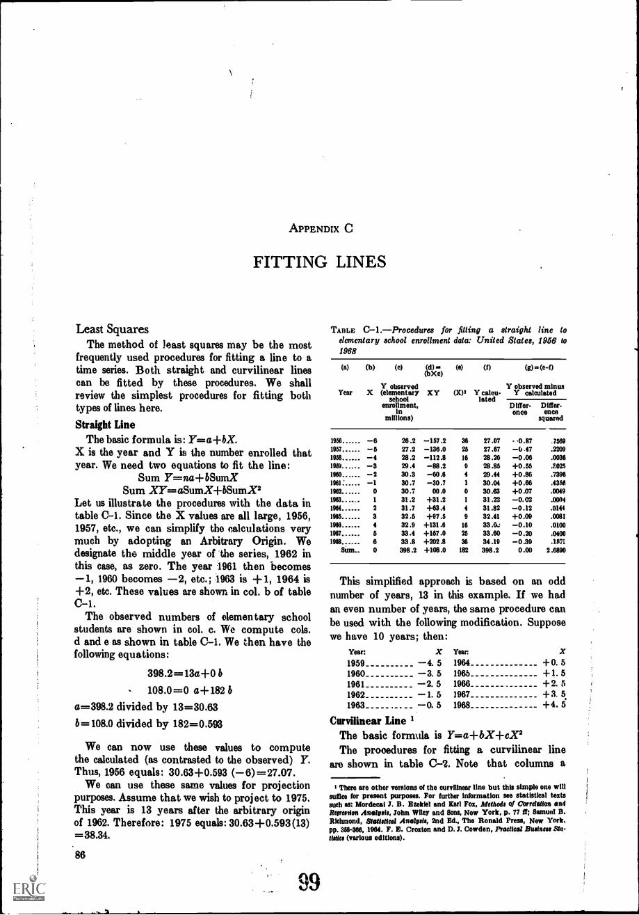
APPENDIX C
FITTING LINES
Least SquaresThe method of least squares may be the most
frequently used procedures for fitting a line to atime series. Both straight and curvilinear linescan be fitted by these procedures. We shallreview the simplest procedures for fitting bothtypes of lines here.
Straight LineThe basic formula is: Y=a+bX.
X is the year and Y is the number enrolled thatyear. We need two equations to fit the line:
Sum Y=nad-bSumXSum XY=a,SumXd-bSumX2
Let us illustrate the procedures with the data intable C-1. Since the X values are all large, 1956,1957, etc., we can simplify the calculations verymuch by adopting an Arbitrary Origin. Wedesignate the middle year of the series, 1962 inthis case, as zero. The year 1961 then becomes-1, 1960 becomes -2, etc.; 1963 is +1, 1964 is+2, etc. These values are shown in col. b of tableC-1.
The observed numbers of elementary schoolstudents are shown in col. c. We compute cols.d and e as shown in table C-1. We then have thefollowing equations:
398.2=13a+0 b108.0=0 a+182 b
a=398.2 divided by 13=30.63b=108.0 divided by 182=0.593
We can now use these values to computethe calculated (as contrasted to the observed) Y.Thus, 1956 equals: 30.63+0.593 (-6)=27.07.
We oan use these same values for projectionpurposes. Assume that we wish to project to 1975.This year is 13 years after the arbitrary originof 1962. Therefore: 1975 equals: 30.63+0.593(13)=38.34.
86
99
TABLE C-1.-Procedures for fitting a straight line toelementary school enrollment data: United States, 1956 to1968
(a)
Year
(b)
X
(c)
Y observed(elementary
schoolenrollment,
inmillions)
Xc)
XY
(0)
(X)3
(0
Y calcu-lated
(g) (e.()
Y observed mMusY calculated
Differ-ence
Differ-ence
squared
1956 -6 26.2 -157.2 36 27.07 - .0.87 .75691957 -5 27.2 -136.0 25 27.87 -6.47 .22091958 -4 28.2 -112.8 16 28.26 -0.06 .00361959 -3 29.4 -88.2 9 28.85 +0.55 .2.025
1980 -2 30 .3 -60.6 4 29 .44 +0 .86 .73961981 -1 30.7 -30.7 1 30.04 +0.66 .43M1982 0 30.7 00.0 0 30.63 +0.07 .0049
1 31.2 +31.2 1 31 .22 -0.02 .00041964 2 31.7 +63.4 4 31.82 -0.12 .01441905 3 32.5 +97.5 9 32.41 +0.09 .00811986 4 32.9 +131.6 16 33.0a -0.10 .01001967 5 33.4 +167.0 25 33.60 -0.20 .04001908 6 33.8 +202A 38 34.19 -0.39 .1521
Mim 0 398.2 +108.0 182 398.2 0.00 2.6890
This simplified approach is based on an oddnumber of years, 13 in this example. If we hadan even number of years, the same procedure canbe used with the following modification. Supposewe have 10 years; then:
Year: X Year:
1959 -4. 5 1964 +0. 51960 -3. 5 1965 +1. 51961 -2. 5 1966 +2. 51962 -1. 5 1967 +3. 5.1963 -0. 5 1968 +4. 5
Curvilinear Line 1The basic formula is Y=a+bXd-cX2The prooedures for fitting a curvilinear line
are shown in table 0-2. Note that columns a
There are other versions of the curvMnear line but this simple one willsuffice tor present purposes. For further information see statistical textssuch as: Mordecai J. B. Ezekiel and Karl Fox, Methods of Corrdation andRepression Anal's*, John Wiley and Bons, New York, p. 77 0; Samuel B.Rkhmond, Statistical Antibiosis, 2nd Ed., The Ronald Press, New York.pp. 358-366, 1964. F. E. Creston and D.J. Cowden, Practical Businen Sta-tistics (various editions).
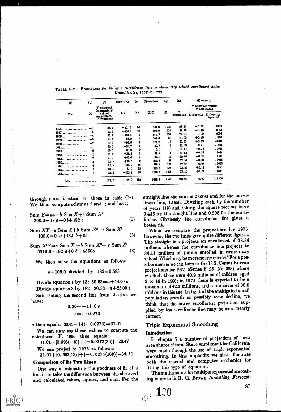
TABLE C-2.-Procedures for fitting a curvilinear line to elementary school enrollment data:United Slates, 1966 to 1968
(a) (b) (c) (d)=(bXc)
Y observed(elementary
X school XYenrollment,in millions)
Year
(0) (cXe) (g) (h) (0= (c-b)Y observed minus
Y calculatedX2 X2Y Xt
calculated Difference Differencesquared
1956 -6 26. 2 -157. 2 36 943. 2 1290 26. 47 -0, 27 . 0729
1957 -5 27. 2 -136.0 25 680. 0 625 27. 36 -O. 16
1958 -4 28. 2 -112. 8 16 451. 2 256 28. 20 0. 00 . 0000
1959 -3 29. 4 -88. 2 9 284. 6 81 29. 00 +0. 40 . /600
1960 -2 30. 3 -60. 6 4 121. 2 16 29. 71 +0. 59 .3481
1961 -1 30. 7 -30. 7 1 30. 7 1 30. 39 +0. 31 . 0961
1962 o 30. 7 00,0 0 O. 0 0 31. 01 -O. 31 . 0961
1963 ... 1 31. 2 +31. 2 1 31. 7 31. 58 -O. 38 . 1444
1964 2 31. 7 +63. 4 4 126.8 16 32. 09 -O. 39 . 1521
1965 3 32. 5 +97. 5 9 292. 5 81 32. 54 -O. 04 . 0016
1966 4 32. 9 +131. 6 16 526. 4 256 32, 95 -0. 05 . 0025
1967 5 33. 4 +167. 0 25 835. 0 625 33. 29 +0. 11 . 0121
1968 ... 6 33. 8 +202. 8 36 1216. 8 1296 33. 59 +0. 21 . 0441
Sum 399. 2 +109. 0 192 5519. 6 4550 398. 20 0. 00 1. 1556
through e are identical to those in table C-1.We then compute columns f and g and have;
Sum Y=na-l-b Sum X-i-c Sum X2398.2=13 a+0 6+182 c (1)
Sum XY=a Sum X-Fb Sum X2-Fc Sum X3108.0=0 a+182 b-1-0c (2)
Sum X2Y=a Sum X2-14 Sum 20-1- c Sum X4
5519.6=182 a+0 b+4550c (3)
We then solve the equations as follows:
b=108.0 divided by 182=0.593
Divide equation 1 by 13: 30.63=a+ 14.00 cDivide equation 3 by 182: 30.33=a+25.00 cSubtrlkcting the second line from the first we
have:0.30=-11.0c
c= -0.0273
a then equals: 30.63- 14(-0.0273)= 31.01We can now use these values to compute the
calculated Y. 1956 thus equals:31.01+ [0.593(- 6)] + [- 0.0273(36)]=26.47
We can project to 1975 as follows:31.01+[0. 593(13)]+ [-O. 0273(169)1=34. 11
Comparison of the Two LinesOne way of estimating the goodness of fit of a
line is to take the difference between the observedand calculated values, square, and sum. For the
straight line the sum is 2.6890 and for the curvi-linear line, 1.1556. Dividing each by the numberof years (13) and taking the square root we have0.455 for the straight line and 0.298 for the curvi-linear. Obviously the curvilinear line gives abetter fit.
When we compare the projections for 1975,however, the two lines give quite different figures.The straight line projects an enrollment of 38.34millions whereas the curvilinear line projects to34.11 millions of pupils enrolled in elementaryschool. Which may b e more nearly correct? For a pos-sible answer we can turn to the U.S. Census Bureauprojections for 1975 (Series P-25, No. 388) wherewe find: there were 40.2 millions of children aged5 to 14 in 1966; in 1975 there is expected to be amaximum of 42.2 millions, and a minimum of 38.5millions in this age. In light of the anticipated smallpopulation growth or possibly even decline, we
think that the lower enrollment projection sup-plied by the curvilinear line may be more nearly
correct.
Triple Exponential SmoothingIntroduction
In chapter 7 a number of projections of localarea shares of total State enrollment for Californiawere made through the use of triple exponentialsmoothing. In this appendix we shall illustrateboth the manual and computer mechanics forfitting this type of equation.
The mathematics for multiple exponential smooth-ing is given in R. G. Brown, Smoothing, Forecast-
IP 087
ing, and Prediction of Discreet Time Series, PrenticeHall, New Jersey, 1963.
This type of equation can be fitted by a com-puter or manually. Considering the large amountof work involved, the former is preferable.
The Computer ProgramThe computer program shown is an IBM
Application Program, System 1360 ScientificSubroutine Package (360A-CM-03X) VersionIII, Programmer's Manual, IBM, TechnicalPublications Department, 112 East Post Road,White Plains, New York, 10601. The reader whomay wish further information may write to theBureau of Applied Social Research, ColumbiaUniversity; every effort will be made to supplysuch information applicable on an IBM 360computer. Following is the IBM description :
Probicm Description.Given a time seriesX, a smoothing constant, and three coefficientsof the prediction equation, this sample programfinds the triple exponentially smoothed series Sof the time series X.
Program Description.The sample programfor triple exponential smoothing consists of themain program named EXPON, and one subroutine,EXSMO, from the Scientific Subroutine Package
Capacity .The capacity of the sample prog.rainand the format required for data input have beenset, up as follows:
1. Up to 1,000 data points in a given time series2. (12F 6.0) format for input data cardsTherefore, if a problem satisfies the above con-
ditions, the sample program need not be modified.However, if there are more than 1,000 data points,the dimension statement in the sample mainprogram must be modified to handle this particularproblem. Similarly, if input data cards are pre-pared using a different format, the input formatin the sample main program must be modified.The general rules for program modification aredescribed later.
Input. Control Card.One con trol card is re-quired for each problem and is read by tbe main pro-gram , EXPON. This card is prepared as follows:
Columns ContentsFor
sampleproblem
1- 6 Problem number (may be alphameric)7-10 Number of data points hi a given time series.
11-15 Smoothing constant, a (0.0<a <1.0)16-25 First coefficient (A) of the prediction equation26-35 Second coefficient (B) of the prediction equation36-45 Third coefficient (C) of the prediction equation
Sample00380.10.00.00.0
88
Smoothing constant, and three coefficients must bekeypunched with decimal points.
Leading zeros are not required to be key-punched.
Data Card.Time series data are keypunchedusing the format (12F6.0). This format assumesthat each data point is keypunched in a 6-cohnnn field and 12 fields per card.
Deck Setup.The deck setup is shown in Figure62. (see p. 89)1
Sample.The listing of input cards for thesample problem is presented in figure 63, p. 89.1Output
Description.The output of the sample pro-gram for triple exponential smoothing includes:
1. Original and updated coefficients2. Time series as input and triple exponentially
smoothed time seriesExample.The output listing for the sample
problem is shown in figure 64, page 91.1Program Modification.Program capacity
can be increased or decreased by making changesin the dimension statement. Input data in a dif-ferent format can also be handled by providing aspecific format statement. In order to familiarizethe user with the program modification, the fol-lowing general rules are supplied in terms of theSample problem.
1. Changes in the dimension statement of themain program, EXPON:
The dimension of arrays X and S must begreater than or equal to the number of data pointsin time series, NX. Since there are 38 data pointsin the sample problem, the value of NX is 38.
2. Changes in the input format statement of themain program, EXPON:
Only the format statement for input data maybe changed. Since sample data are three-digit num-bers, rather than using six-column fields as in thesample problem, each data point may be key-punched in a three-column field and 24 fields percard. If so, the format is changed to (24F3.0).
Operating Instructions.The sample pro-gram for triple exponential smoothing is a standardFORTRAN program. Special operating instruc-tions are not required. Data set 5 is used for input,and data set 6 is used for output.
Timing.The execution time of this sampleprogram on a System/360, Model 30, using anIBM 2540 Card Reader as input and an 1BM 1403,Model 3 as output, is 12 seconds.
The Nos. 62, 63, and 64 used hero reflect the numbering of figures in the
r inal IBM document.t
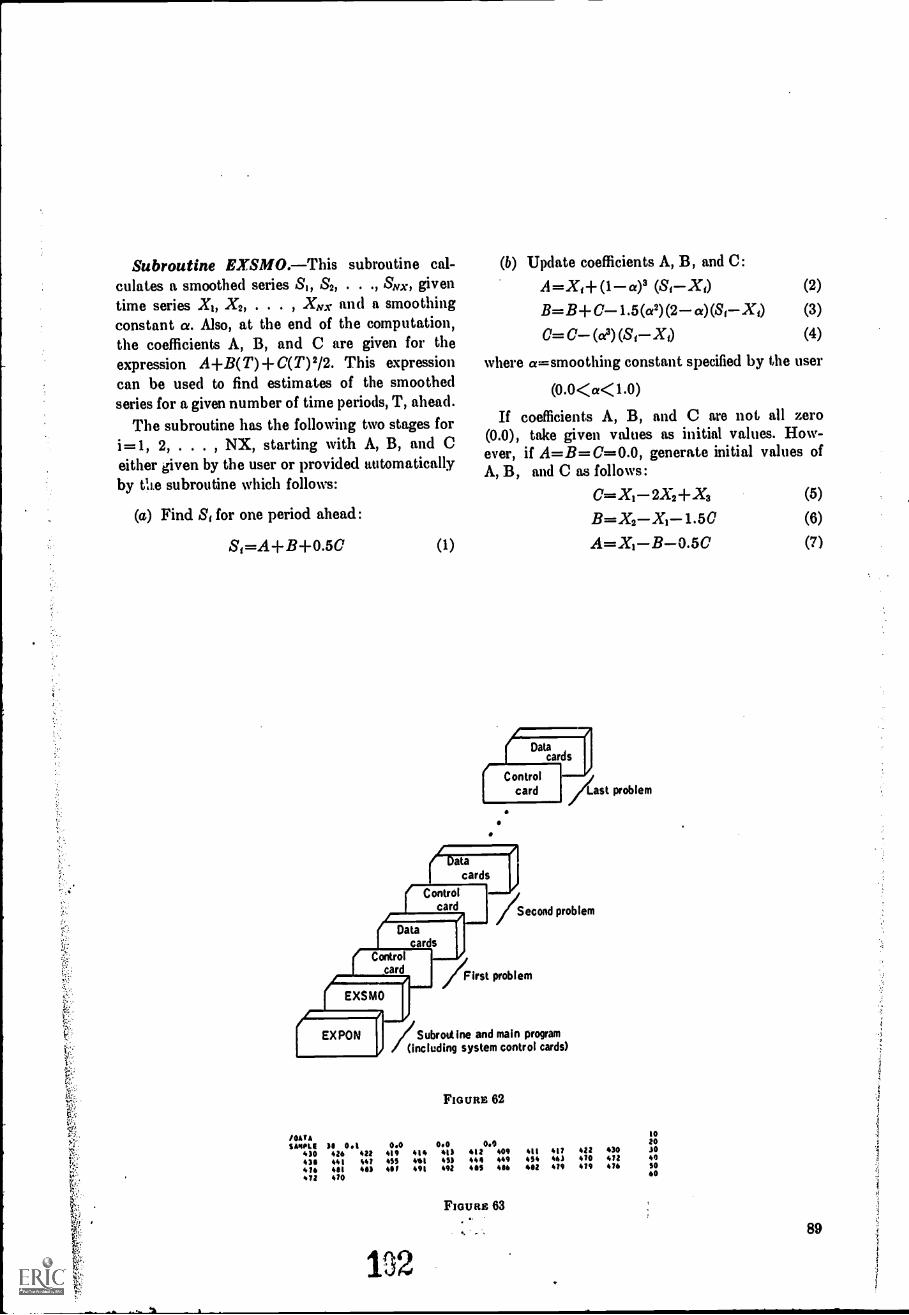
717',
Subroutine EXSMO.This subroutine cal-culates a smoothed series S1 , S2, . . SNX, given
time series Xi, X2, , XNx and a smoothingconstant a. Also, at the end of the computation,the coefficients A, B, and C are given for theexpression A+B(T)+C(T)2/2. This expressioncan be used to find estimates of the smoothedseries for a given number of time periods, T, ahead.
The subroutine has the following two stages fori=1, 2, . . . , NX, starting with A, B, and Ceither given by the user or provided automaticallyby tiae subroutine which follows:
(a) Find S, for one period ahead:
S1=A+B+0.5C (1)
(b) Update coefficients A, B, and C:
A=Xt+ (1 ce)3 (Si Xi)B.B+C-1.5 (a2) (2 a) (S,
C (a3) (Si Xi)
(2)
(3)
(4)
where a=smoothing constant specified by the user
(0.0 <a< 1.0)
If coefficients A, B, and C are not all zero(0.0), take given values as initial values. How-ever, if A=B= C=0.0, generate initial values ofA, B, and C as follows:
2X2 + X3 (5)
B=X2X1-1.50A=X1B-0.5C
Controlcard
/Second problem
/First problem
/ Submit ine and main program(including system control cards)
FIGURE 62
/00 ASAMPLE 58 0 .1 0.0 0.0 0.0 20
430 426 472 419 414 415 412 409 411 417 422 430 30
458 441 447 455 461 455 446 449 454 465 470 472 40
476 481 483 467 491 492 485 486 482 479 479 476 SO
72 470 60
132
Flew as 63
(6)
(7)
89
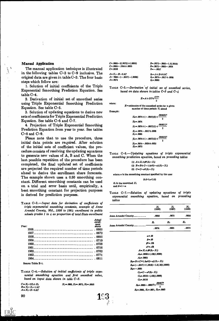
Manual ApplicationThe manual application technique is illustrated
in the following tables C-3 to 0-9 inclusive. Theoriginal data are given in table 0-3. The four basicsteps which follow are:
1. Solution of initial coefficients of the TripleExponential Smoothing Prediction Equation. Seetable C-4.
2. Derivation of initial set of smoothed seriesusing Triple Exponential Smoothing PredictionEquation. See table C-5.
3. Solution of updating equations to derive newsets of coefficients for Triple Exponential PredictionEquation. See table C-6 and 0-7.
4. Projection of Triple Exponential SmoothingPrediction Equation from year to year. See tables0-8 and C-9.
Please note that to use the procedure, threeinitial data points are required. After solutionof the initial sets of coefficient values, the pro-cedure consists of resolving the updating equationsto generate new values of A, B and C. When thelast possible repetition of the procedure has beencompleted, the final updated set of coefficientsare projected the required number of time periodsaheacl to derive the enrollment share forecasts.The example shown uses a 0.50 smoothing con-stant. Different smoothing constants can be usedon a trial and error basis until, empirically, abest smoothing constant for projection purposesis derived for prediction purposes.
TABLE C-3.-Input data for derivation of coefficients oftriple exponential smoothing constants, example of AnneArundel County, Md., 1966 to 1964: enrollment in publicschools grades 1 to 4 as proportion of total State enrollment
Year:
Adualenroll-mentshares
1956 . 06651957 06721958 06951959 07191960 . 07381961 07561962 . 07621963 . 07711964 0811
Source: Table E-1.
TABLE C-4.-Solution of initial coefficients of triple expo-nential smoothing equation and first smoothed value,based on input data shown in table C-3.
Cm Xt-,2X2+ X3Xa-- X1- I .5CXt--13-0.50
90
Xt.. .0665, X2...0672, X3 .0695
C=.0665-2(.0672)+(.0695) Bm.0272-.0665-1.5(.0016)Cm.0665-.1344+.0695 B..0672-.06435--.0024Cm.0016 -.0017
A., XI-B-0.5C A+ B+0.5CA.- .0665- (-.0017)- (.0008) A...0674-.0017+ .0008A-.0674 Sim.0665
TABLE C-5.-Derivation of initial set of smoothedbased on data shown in tables C-3 and C-4
where:
Example:
:E=A+BT-F---CT2
Emestimates of the smoothed series for a givennumber of time periods 21 ahead
Eom.0674+(-.0017)(0)+2
Eo=..0674
.0016(0)2
Etm.0674+(-.0017)(1)+2
.0016(1)2
EI=.0674- .00174-.0008=.0665
Eo=.0674+(-.0017)(2)+2
.0016(2)2
A=.0674-.0034+.0032E2=.0672
series,
TABLE C-6.-Updating equations of triple exponentialsmoothing prediction equation, based on preceding tables
Xt-fp3(St- Xi)(2) B=13+ C- 1.5a7(2- a)(Sr- X r)(3) C...C-ora(Si-- Xi)
where a is the smoothing constant specified by the user
(0.0<a<1.0)
St is the smoothed Xrand e3.1-es
TABLE C-7.-Solution of updating equations of tripleexponential smoothing equation, based on precedingtabl es
XI X2 X3(1956) (1957) (1958)
Anne Arundel County .0665 .0672 .0695
Anne Arundel CountyEl E3 E3
.0674 .0665 .0672
p..so0-.125ah..125
A.2c1+10(81- Xi)Ao-.0665+(.125)(.0000)
Awe .0885
Bo.. B+C. 1.500(2- a) (Si - XI)
( - .0017) + (.0018)- 1.5(.25) (.0000)
Be. -.0001Co... - ora(Si- Xi)C'e .0018- (.I25) (.0000)
Cop..00113
.00113TISim .0885-.0002T+
2
am .0885, St .0871, Sp..0893
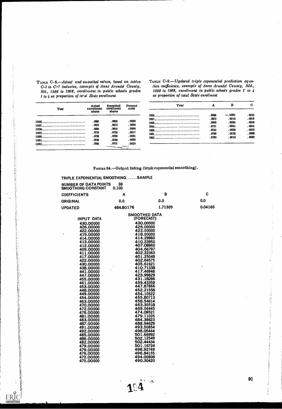
TAM; C-8.-Aclual and smoothed values, based on tablesC-3 to C-7 inclusive, example of Anne Arundel County,Md., 1066 to 1962, enrollment in public schools grades1 to 4 as proportion of to!al State enrollment
YearActual
enrollmentshares
Smoothedenrollment
shares
1956 .0605 .0665
1957 .0672 .0672
1958 .0695 .0695
1959 .0719 .0730
1960 .0738 .0769
1961 .0756 .0780
1002 .0702 .0791
Percenterror
.0000
.0000
.0000
.0017
.0031
.0030
.0029------,-_--
TABLE C-9.-Updaled triple exponential prediction equa-tion coefficients, example of Anne Arundel County, Md.,1066 to 1062, enrollment in public schools grades 1 tv 4as proportion of total Slate enrollmeni
Year
1956
1957
1958
1959
1960
1961
1962
A II
.0665 -.6001 . 0010
.0672 .0015 . 0010
.0695 .0034 . 0016
.0721 . 0041 . 0014
.0742 .0039 .0010
.0760 .0028 . 0000
.0765 . 0016 . 0002
FIGURE 64.-Output listing (triple exponential smoothing).
TRIPLE EXPONENTIAL SMOOTHING SAMPLE
NUMBER OF DATA POINTSSMOOTH I N G .00 NSTANT
COEFFICIENTS
ORIGI NAL
UPDATED
I N PUT DATA430.00000426.00000422.00000419.00000414.00000413.00000412.00000409.00000411.00000417.00000422.00000430.00000438.00000441.00000447.00000455.00000461.00000453.00000448.00000449.00000454.00000463.00000470.00000472.00000476.00000481.00000483.00000487.00000491.00000492.00000485.00000486.00000482.00000479.00000479.00000476.00000472.00000470.00000
380.100
A
0.0
484.80176
0.0 0.0
1.71309 0.04166
SMOOTHED DATA(FORECAST)430.00000426.00000422.00000418.00000414.29980410.23950407.08960404.66797402.22363401.25049402.64575405.61621410.71338417.46948423.99829431.18286439.43359447.87866452.21558454.10522455.80713458.54614463.30518469.06445474.09521479.11035484.38623488.94629493.50854498.05444501.66992502.12549502.44434501.16724498.92749496.84155494.00806490.30420
91
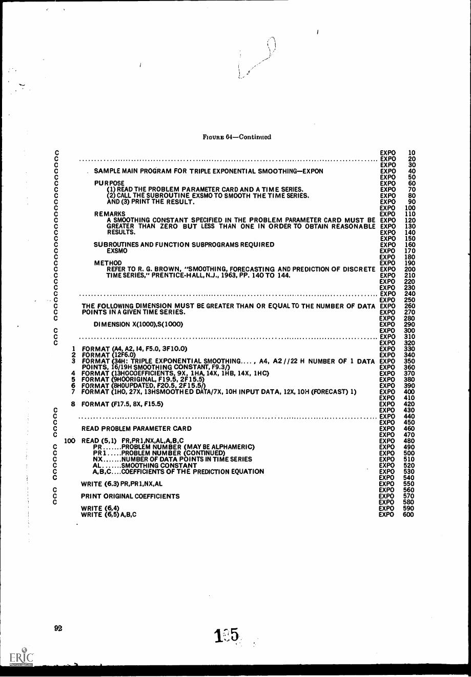
FIGURE 04Contintied
CCC
EXPOEXPOEXPO
102030
C SAMPLE MAIN PROGRAM FOR TRIPLE EXPONENTIAL SMOOTHINGEXPON EXPO 40C EXPO 50C PURPOSE EXPO 60C (1) READ THE PROBLEM PARAMETER CARD AND A TIME SERIES. EXPO 70C (2) CALL THE SUBROUTINE EXSMO TO SMOOTH THE TI ME SERIES. EXPO 80C AND (3) PRINT THE RESULT. EXPO 90C EXPO 100C REMARKS EXPO 110C A SMOOTHING CONSTANT SPECIFIED IN THE PROBLEM PARAMETER CARD MUST BE EXPO 120C GREATER THAN ZERO BUT LESS THAN ONE IN ORDER TO OBTAIN REASONABLE EXPO 130C RESULTS. EXPO 140C EXPO 150C SUBROUTINES AND FUNCTION SUBPROGRAMS REQUIRED EXPO 160C EXSMO EXPO 170C EXPO 180C METHOD EXPO 190C REFER TO R. G. BROWN, "SMOOTHING, FORECASTING AND PREDICTION OF DISCRETE EXPO 200C TIME SERIES," PRENTICE-HALL, N.J., 1963, PP. 140 TO 144. EXPO 210C EXPO 220C EXPO 230C EXPO 240C EXPO 250C THE FOLLOWING DIMENSION MUST BE GREATER THAN OR EQUAL TO THE NUMBER OF DATA EXPO 260C POINTS IN A GIVEN TIME SERIES. EXPO 270C EXPO 280
DIMENSION X(1000),S(1000) EXPO 290C EXPO 300C EXPO 310C EXPO 320
1 FORMAT (A4, A2,14, F5.0, 3F10.0) EXPO 3302 FORMAT (12F6.0) EXPO 3403 FORMAT (34H: TRIPLE EXPONENTIAL SMOOTHING.... , A4, A2 / / 22 H NUMBER OF 1 DATA EXPO 350
POINTS, 16/19H SMOOTHING CONSTANT, F9.3/) EXPO 3604 FORMAT (13HOCOEFFICIENTS, 9X, 1HA, 14X, 1HB, 14X, 1HC) EXPO 3705 FORMAT (9HOORIGINAL, F19.5, 2F15.5) EXPO 3806 FORMAT (8HOUPDATED, F20.5, 2F15.5/) EXPO 3907 FORMAT (1HO, 27X, 13HSMOOTH ED DATA/7X, 10H INPUT DATA, 12X, 10H (FORECAST) 1) EXPO 400
EXPO 4108 FORMAT (F17.5, 8X, F15.5) EXPO 420
C EXPO 430C EXPO 440C EXPO 450C READ PROBLEM PARAMETER CARD EXPO 460C EXPO 470
100 READ (5,1) F'R,PR1,NX,AL,A,B,C EXPO 480C PR PROBLEM NUMBER (MAY BE ALPHAMERIC) EXPO 490C PR 1 PROBLEM NUMBER (CONTINUED) EXPO 500C NX NUMBER OF DATA POINTS IN TIME SERIES EXPO 510C AL SMOOTHING CONSTANT EXPO 520C A,B,C....COEFFICIENTS OF THE PREDICTION EQUATION EXPO 530C EXPO 540
WRITE (6.3) PR,PR1,NX,AL EXPO 550C EXPO 560C PRINT ORIGINAL COEFFICIENTS EXPO 570C EXPO 580
WRITE (6,4) EXPO 590WRITE (6,5) A,B,C EXPO 600
92 -
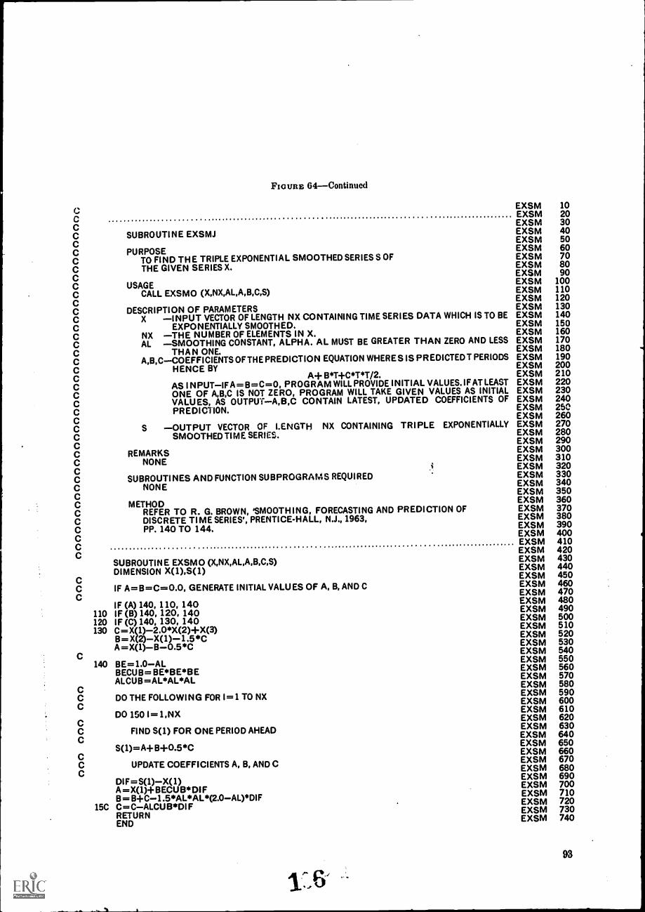
FIGURE 64Continued
CCC
EXSMEXSMEXSM
102030
C SUBROUTINE EXSMJ EXSM 40
CEXSM 50
C PURPOSE EXSM 60
C TO FIND THE TRIPLE EXPONENTIAL SMOOTHED SERIES S OF EXSM 70
C THE GIVEN SERIES X. EXSM 80
CEXSM 90
C USAGE EXSM 100
C CALL EXSMO (X,NX,AL,A,B,C,S) EXSM 110
CEXSM 120
C DESCRIPTION OF PARAMETERS EXSM 130
C X -INPUT VECTOR OF LENGTH NX CONTAINING TIME SERIES DATA WHICH IS TO BE EXSM 140
C EXPONENTIALLY SMOOTHED. EXSM 150
C NX -THE NUMBER OF ELEMENTS IN X. EXSM 160
C AL -SMOOTHING CONSTANT, ALPHA. AL MUST BE GREATER THAN ZERO AND LESS EXSM 170
C THAN ONE. EXSM 180
C A,B,C-COEFFICIENTS OF THE PREDICTION EQUATION WHERE S IS PREDICTED T PERIODS EXSM 190
C HENCE BY EXSM 200
C A+ B*Ti-C*T*T/2. EXSM 210
C AS I N PUT-IF A= B= C=0, PROGRAM WILL PROVIDE INITIAL VALUES. IF AT LEAST EXSM 220
C ONE OF A,B,C IS NOT ZERO, PROGRAM WILL TAKE GIVEN VALUES AS INITIAL EXSM 230
C VALUES, AS OUTPUT-A,B,C CONTAIN LATEST, UPDATED COEFFICIENTS OF EXSM 240
C PREDIC1ION. EXSM 250
CEXSM 260
C S -OUTPUT VECTOR OF LENGTH NX CONTAINING TRIPLE EXPONENTIALLY EXSM 270
C SMOOTHED TIM E SERIES. EXSM 280
CEXSM 290
C REMARKS EXSM 300
C NONE EXSM 310
CEXSM 320
C SUBROUTINES AND FUNCTION SUBPROGRAMS REQUIRED EXSM 330
C NONE EXSM 340
CEXSM 350
C METHOD EXSM 360
C REFER TO R. G. BROWN, 'SMOOTHING, FORECASTING AND PREDICTION OF EXSM 370
C DISCRETE TIME SERIES', PRENTICE-HALL, N.J., 1963, EXSM 380
C PP. 140 TO 144. EXSM 390
CEXSM 400
CEXSM 410
CEXSM 420
SUBROUTINE EXSMO (X,NX,AL,A,B,C,S) EXSM 430
DIMENSION X(1),S(1) EXSM 440
CEXSM 450
C IF A=B=C=0.0, GENERATE INITIAL VALUES OF A, B, AND C EXSM 460
CEXSM 470
IF (A) 140, 110, 140 EXSM 480
110 IF (B) 140, 120, 140 EXSM 490
120 IF (C) 140, 130, 140 EXSM 500
130 C=X(1)-2.0*X(2)+X(3) EXSM 510
B=X(2)-X(1)-1.5*C EXSM 520
A = X(1)-B-0.5*C EXSM 530
CEXSM 540
140 BE=1.0-AL EXSM 550
BECUB=BE*BE*BE EXSM 560
ALCUB=AL*AL*AL EXSM 570
CEXSM 580
C DO THE FOLLOWING FOR I = 1 TO NX EXSM 590
CEXSM 600
DO 150 I= 1,NX EXSM 610
CEXSM 620
C FIND S(1) FOR ONE PERIOD AHEAD EXSM 630
C EXSM 640
S(1)=A+B4-0.5*C EXSM 650
CEXSM 660
C UPDATE COEFFICIENTS A, B, AND C EXSM 670
CEXSM 680
DIF=S(1)-X(1) EXSM 690
A=X(1)+BECUB*DIF EXSM 700
B= Bi-C-1.5*AL*AL*(2.0-AL)*DIF EXSM 710
15C C=C-ALCUB*DIF EXSM 720
RETURNEXSM 730
ENDEXSM 740
93
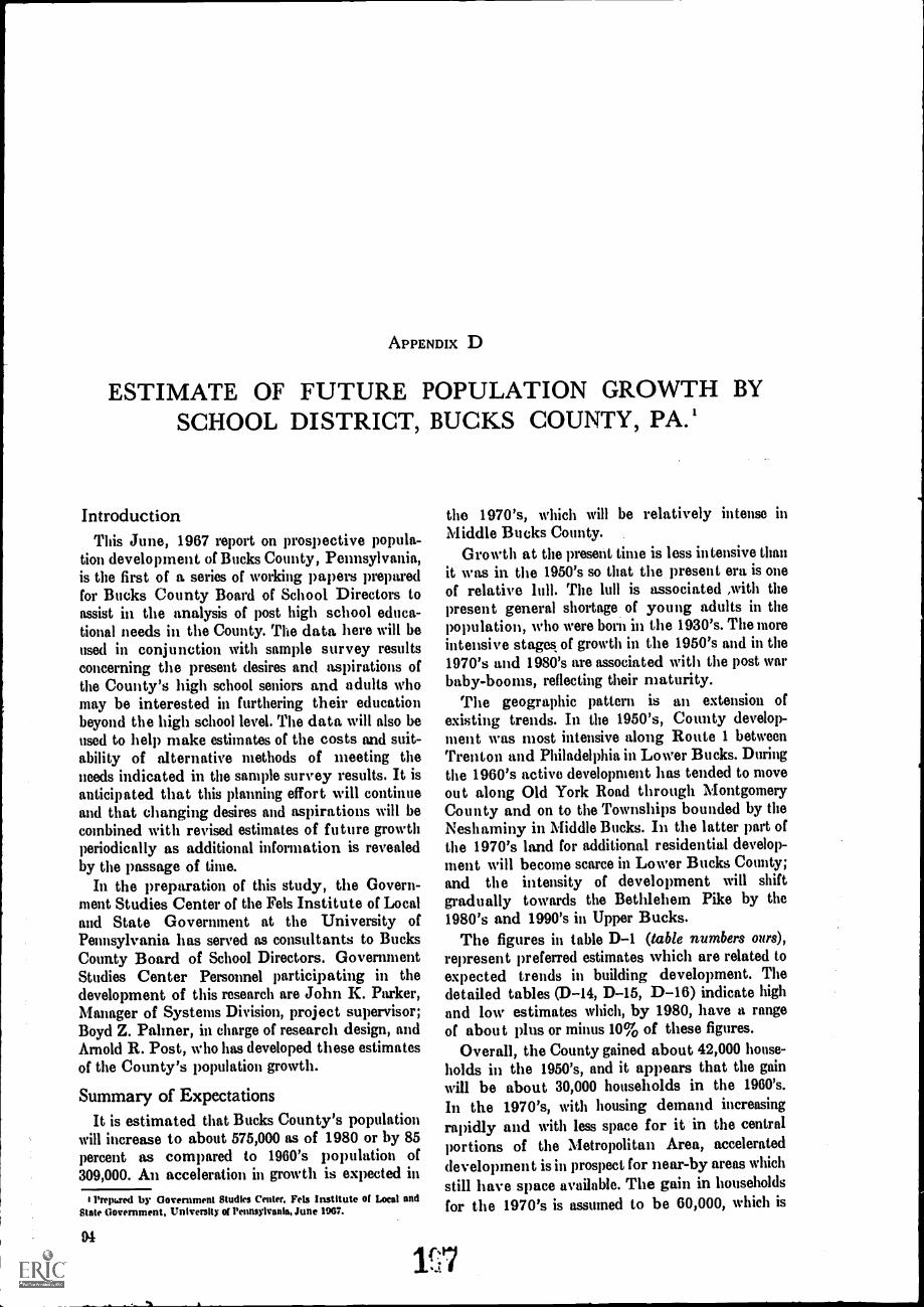
APPENDIX D
ESTIMATE OF FUTURE POPULATION GROWTH BYSCHOOL DISTRICT, BUCKS COUNTY, PA.'
IntroductionThis June, 1967 report on prospective popula-
tion development of Bucks County, Pennsylvania,is the first of a series of working papers preparedfor Bucks County Board of School Directors toassist in the analysis of post high school educa-tional needs in the County. The data here will beused in conjunction with sample survey resultsconcerning the present desires and aspirations ofthe County's high school seniors and adults whomay be interested in furthering their educationbeyond the high school level. The data will also beused to help make estimates of the costs and suit-ability of alternative methods of meeting theneeds indicated in the sample survey results. It isanticipated that this planning effort will continueand that changing desires and aspirations will becombined with revised estimates of future growthperiodically as additional information is revealedby the passage of time.
In the preparation of this study, the Govern-ment Studies Center of the Fels Institute of Localand State Government at the University ofPennsylvania has served as consultants to BucksCounty Board of School Directors. GovernmentStudies Center Personnel participating in thedevelopment of this research are John K. Parker,Manager of Systems Division, project supervisor;Boyd Z. Pahner, in charge of research design, andArnold R. Post, who has developed these estimatesof the County's population growth.
Summary of ExpectationsIt is estimated that Bucks County's population
will increase to about 575,000 as of 1980 or by 85percent as compared to 1960's population of309,000. An acceleration in growth is expected in
Prem.red by Government Studies Center, Feb Institute of Local andStale Government, University of Pennsylvania, June 1967.
94
the 1970's, which will be relatively intense inMiddle Bucks County.
Growth at the present time is less intensive thanit was in the 1950's so that the present era is oneof relative lull. The lull is associated ,with thepresent general shortage of young adults in thepopulation, who were born in the 1930's. The moreintensive stages of growth in the 1950's and in the1970's and 1980's are associated with the post warbaby-booms, reflecting their maturity.
The geographic pattern is an extension ofexisting trends. In the 1950's, County develop-ment was most intensive along Route 1 betweenTrenton and Philadelphia in Lower Bucks. Duringthe 1960's active development has tended to moveout along Old York Road through MontgomeryCounty and on to the Townships bounded by theNeshaminy in Middle Bucks. In the latter part ofthe 1970's land for additional residential develop-ment will become scarce in Lower Bucks County;and the intensity of development will shiftgradually towards the Bethlehem Pike by the1980's and 1990's in Upper Bucks.
The figures in table D-1 (table numbers ours),represent preferred estimates which are related toexpected trends in building development. Thedetailed tables (D-14, D-15, D-16) indicate highand low estimates which, by 1980, have a rangeof about plus or minus 10% of these figures.
Overall, the County gained about 42,000 house-holds in the 1950's, and it appears that the gainwill be about 30,000 households in the 1960's.In the 1970's, with housing demand increasingrapidly and with less space for it in the centralportions of the Metropolitan Area, accelerateddevelopment is in prospect for near-by areas whichstill have space available. The gain in householdsfor the 1970's is assumed to be 60,000, which is
1"7
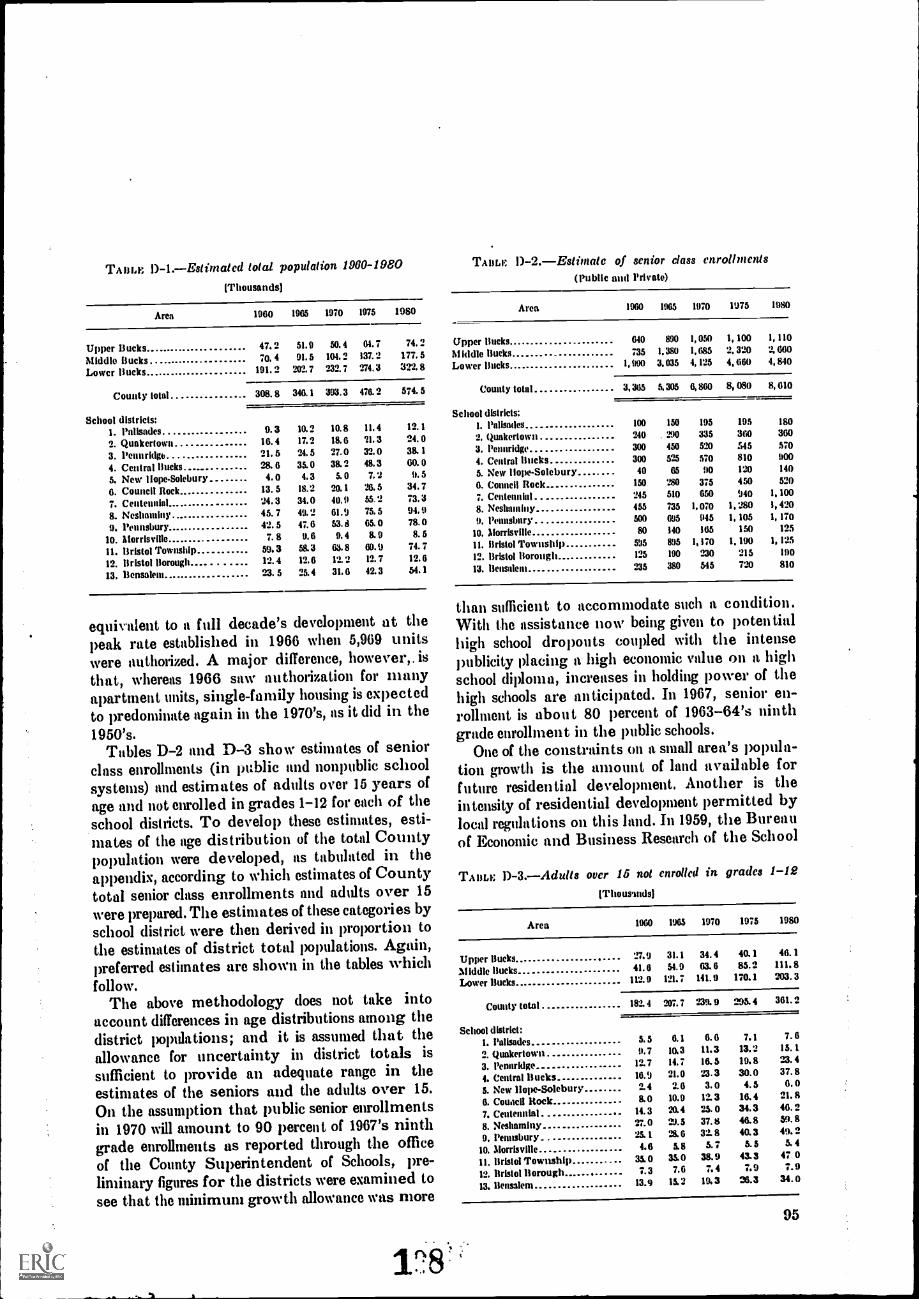
TA BLE D-1.-Estimated total population 1960-1980
(Thousands)
Area 1960 1965 1970 1975 1980
Upper Bucks 47. 2 51.9 50. 4 64. 7 74. 2
Middle Bucks 70. 4 91. 5 104. 2 137. 2 177. 5
Lower Ducks 101. 2 202. 7 232. 7 274. 3 322. 8
County total 308. 8 346. 1 393.3 476.2 574. 5
School districts:1. Palisades 9. 3 10. 2 10.8 II. 4 12. 1
2. Quakertown 16. 4 17.2 18. 6 11.3 24. 0
3. Penn Mgt, 21. 5 24. 5 27.0 32.0 38. 1
4. Central Bucks 28. 6 35. 0 38. 2 48. 3 GO. 0
5. New 1 lope-Solebury 4. 0 4.3 5. 0 7. 2 9. 5
6. Council Rock 13. 5 18. 2 20. 1 26. 5 34. 7
7. Centennial 24.3 34.0 40.9 55.2 73. 3
8. Neshaminy 45. 7 49.2 61.9 75, 5 94. 9
9. Pennsbury 42. 5 47. 6 53. 8 65. 0 78.0
10. Morrisville 7. 8 9.6 9. 4 8. 9 8. 5
11. Bristol Township 59. 3 58. 3 63.8 69.9 74. 7
12. Bristol Borough 12. 4 12.6 12. 2 12. 7 12. 6
13. Bensalem.. =. 5 25.4 31. 6 42.3 54. 1
equivalent to a full decade's development at thepeak rate established in 1966 when 5,969 unitswere authorized. A major difference, however,, isthat, whereas 1966 saw authorization for manyapartment units, single-family housing is expectedto predominate again in the 1970's, as it did in the1950's.
Tables D-2 and D-3 show estimates of seniorclass enrollments (in public and nonpublic schoolsystems) and estimates of adults over 15 years of
age and not enrolled in grades 1-12 for each of theschool districts. To develop these estimates, esti-mates of the age distribution of the total Countypopulation were developed, as tabulated in theappendix, according to which estimates of Countytotal senior class enrollments and adults over 15were prepared. The estimates of these categories byschool district were then derived in proportion tothe estimates of district total populations. Again,preferred estimates are shown in the tables whichfollow.
The above methodology does not take intoaccount differences in age distributions among thedistrict populations; and it is assumed that theallowance for uncertainty in district totals issufficient to provide an adequate range in theestimates of the seniors and the adults over 15.
On the assumption that public senior enrollmentsin 1970 will amount to 90 percent of 1967's ninthgrade enrollments as reported through the officeof the County Superintendent of Schools, pre-liminary figures for the districts were examined tosee that the minimum growth allowance was more
1 8,
TAnLE D-2.--Estimalc of senior class enrollments(Public aud Private)
Area 1960 1965 1970 1975 1980
Upper Bucks 640 890 1, 050 1, 100 I, 110
Middle liuckq 735 1.380 I, 685 2, 320 2, 660
Lower Bucks 1, 990 3.035 4, 125 4, 660 4, 840
County total 3, 365 5, 305 6, 860 8, 080 8, 610
School districts:I. Palisades 100 150 195 195 180
2. Quakertown 240 290 335 360 360
3. Penuridge 300 450 520 545 570
4. Central Bucks 300 525 570 810 900
5. New I lope-Solehury 40 65 90 120 140
6. Council Rock 150 280 375 450 520
7. Centennial . 245 510 650 940 I, 100
8. Neshaminy 455 735 1.070 1, 280 1, 420
9. Penusbury 500 695 045 1, 105 1, 170
10. Morrisville 80 140 165 150 125
11. Bristol Township 595 895 1,170 1, 190 1, 125
12. Bristol Borough 125 190 230 215 190
13. Bensalem 235 380 545 720 810
than sufficient to accommodate such a, condition.With the assistance now being given to potentialhigh school dropouts coupled with the intensepublicity placing a high economic value on a highschool diploma, increases in holding power of thehigh schools are anticipated. In 1967, senior en-rollment is about 80 percent of 1963-64's ninthgrade enrollment in the public schools.
One of the constraints on a small area's popula-tion growth is the amount of land available forfuture residential development. Another is theintensity of residential development permitted bylocal regulations on this land. In 1959, the Bureauof Economic and Business Research of the School
TA OLE D-3.-Adulls over 15 not enrolled in grades 1-12(Thousands)
Area 1960 1965 1970 1975 1980
Upper Bucks 27, 9 31.1 34. 4 40. 1 46. 1
Middle Bucks 41.6 54.9 63.6 85.2 111.8
Lower Bucks 112. 9 121.7 141.9 170. 1 203. 3
County total 182. 4 207. 7 239. 9 295. 4 361. 2
School district:1. Palisades 5. 5 6.1 6. 6 7.1 7. 6
2. Quakertown 9.7 10.3 113 13. 2 15. 1
3. Pennridge 12.7 14.7 16.5 19.8 M. 4
4. Central Bucks 16.9 21.0 12.3 30.0 37. 8
5. New llope-Solebury 2.4 2.6 3. 0 4.5 6. 0
6. Coulicil Rock 8.0 10.9 12.3 16.4 21. 8
7. Centennial . 14.3 20.4 25. 0 34.3 46. 2
8. Neshaminy 27.0 23.5 37.8 46.8 59. 8
9. Penusbury 25. 1 24 6 31 8 40. 3 49. 2
10. Morrisville 4,6 5.6 £7 5.5 5.4
Bristol Township 35.0 35.0 38.9 43.3 47 0
12. Bristol Borough 7.3 7.6 7.4 7.9 7.9
13. Bensalem 13.9 15. 2 19.3 33.3 34. 0
95
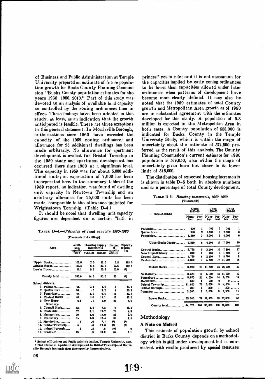
of Business and Public Administration at TempleUniversity prepared an estimate of future popula-tion growth for Bucks County Planning Commis-sion "Bucks County population estimates for theyears 1965, 1980, 2010." Part of this study wasdevoted to an analysis of available land capacityas controlled by the zoning ordinances then ineffect. These findings have been adopted in thisstudy, at least, as an indication that the growthanticipated is feasible. There are three exceptionsto this general statelnent. In Morrisville Borough,authorizations since 1960 have exceeded thecapacity of the 1959 zoning ordinance; andallowance for 25 additional dwellings has beenmade arbitrarily. No allowance for apartmentdevelopment is evident for Bristol Township inthe 1959 study and apartment development hasoccurred there since 1960 at a significant level.The capacity in 1959 was for about 5,000 addi-tional units; an expectation of 7,600 has beenincorporated here. In the summary tables of the1959 report, no indication was found of dwellingunit capacity in Newtown Tewnship and anarbitfary allowance for 15,000 units has beenmade, comparable to the allowance indicated forWrightstown Township. (Table D-4.)
It should be noted that dwelling unit capacityfigures are dependent on a certain "faith in
TABLE D-4.-Uliization of land capacity 1960-1980(Thousands of dwellings)
AreaAvail-
ablecapacity
1960 I
Housing supplyincrements
Percent Capacityof remai n-
capacity ingutilized1960-64 1960-80
Upper BucksMiddle BucksLower Bucks
County total
126.0150. 5
59. 1
2. 06. 65. 7
11. 037. 750. 3
7.822.695.0
115. 0112. 8
(t)
335.6 14.3 99. 0 30 (3)
School districts:1. Palisades 43. 0.4 1.4 3 41. 62. Quakertown 34. . 5 3. 2 8 30.83. Pennridge .. 49. 1.1 6.4 12 42. 64. Central Bucks 59. 2. 0 11.1 17 47.95. New Hope- 6. 5 .1 1.9 26 4.6
Solebury.6. Council Rock 63. 1.4 7. 5 9 55.57. Centennial 72. 3.1 17.2 71 4.88. Neshaminy 20. 1.6 17.0 82 3.09. Pennsbury 15 1.8 13. 5 81 1. 5
10. Morrisville . 5 .6 2. 7 (3) (3)
11. Bristol Township 5. .8 : 7. 6 (3) (3)
12. Bristol Borougk . 6 .2 .6 100 013. Bensalem 18. .9 10.9 65 7.1
t School of Business and l'ublic Administration, Temple University, 1959.2 Not available. Apartment development in Bristol Township and Morris-
ville Borough has made these 1939 capacity figures obsolete.
96
princes" yet to rule; and it is not uncommon forthe capacities implied by early zoning ordinancesto be lower than capacities allowed under laterordinances when patterns of developinent havebecolne more clearly defined. It may also benoted that the 1959 estimates of total Countygrowth and Metropolitan Area growth as of 1980are in substantial agreement with the estimatesdeveloped for this study. A population of 5.8million is expected in the Metropolitan Area inboth cases. A County population of 558,000 isindicated for Bucks County in the TempleUniversity Study, which is within the range ofuncertainty about the estimate of 574,500 pre-ferred as the result of this analysis. The CountyPlanning Commission's current estimate for 1980population is 539,650, also within the range ofuncertainty given here but closer to its lowerlimit of 515,000.
The distribution of expected housing incrementsis shown in table D-5 both in absolute numbersand as a percentage of total County development.
TABLE 1)-5.-Housing increments, 1950-1980(Thousands)
School district
Units195040
Units1960-70
Units1970-80
Nuni- Per-ber cent
Nuni- Per- Num- Per-ber cent ber cent
Palisades 490 1 700 2 700 1
Quakertown 980 2 1,100 3 2, 100 3l'en nridge 1,340 3 2, 200 6 4,200 6
Upper Bucks County 2, 810 6 4,000 12 7,000 10
Central Bucks 2, 720 6 3,300 10 7,800 12
New llope-Solebury 370 1 400 1 1,500 2Council Rock 1, 770 4 2,300 7 5, 200 8Centennial 4, 060 9 5, 500 17 11,700 18
Middle Bucks 8, 920 20 11, 500 35 26, 200 40
Neshaminy 8, 570 19 6,000 18 11,000 17
Pennsbury 8,870 20 4, 500 14 9,000 14
Morrisville 600 1 700 2 0Bristol Township 11, 620 VI 3,000 9 4,600 7
Bristol Borough 280 1 300 1 300Bensalem 3,300 7 3,000 9 7,900 12
Lower Bucks 33, 240 74 17, 500 53 32,800 50
County total 44,970 100 33,000 100 60, 000 100
MethodologyA Note on Method
This estimate of population growth by schooldistrict in Bucks County depends on a methodol-ogy which is still under development but is con-sistent with results produced by special censuses
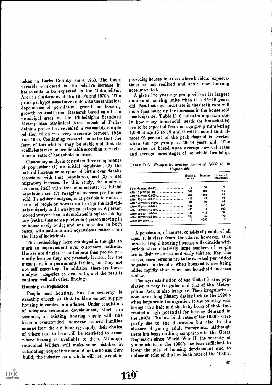
taken in Bucks County since 1960. The basicvariable considered is the relative increase inhouseholds to be expected in the MetropolitanArea in the decades of the 1960's and 1970's. Theprincipal hypotheses have to do with the statisticaldependence of population growth on housinggrowth by small area. Research based on all themunicipal areas in the Philadelphia StandardMetropolitan Statistical Area outside of Phila-delphia proper has revealed a reasonably simplerelation which was very accurate between 1950and 1960. Continuing research indicates that theform of this relation may be stable and that itscoefficients may be predictable according to varia-tions in rates of household increase.
Customary analysis considers three componentsof population: (1) an initial population, (2) thenatural increase or surplus of births over deathsassociated with that population, and (3) a netmigratory increase. In this study, the analysisconcerns itself with two components: (1) initialpopulation and (2) marginal increase per house-hold. In neither analysis, is it possible to make acount of people or houses and assign the individ-uals uniquely to the analytical categories. A personmoved away or a house demolished is replaceable byany (rather than some particular) person moving inor house newly built; and one must deal in bothcases, with patterns and equivalents rather thanthe fate of individuals.
The methodology here employed is thought tomark an improvement over customary. methods.Houses are simpler to anticipate than people pri-marily because they are precisely located, for themost part, in a permanent fashion, and they arenot self generating. In addition, there are feweranalytic categories to deal with, and the resultsconform well with other findings.
Housing vs. PopulationPeople need housing, but the economy is
exacting enough so that builders cannot supplyhousing in careless abundance. Under conditionsof adequate economic development, which areassumed, an existing housing supply will no tbecome overcrowded; however, as new familiesemerge from the old housing supply, their choiceof where next to live will be restricted to areaswhere housing is available to them. Althoughindividual builders will make some mistakes inestimating prospective demand for the houses theybuild, the industry as It whole will »ot persist in
providing houses in areas where builders' expecta-tions are not realized and actual new housinggoes unwanted.
A given five year age group will use its largestnumber of housing units when it is 45-49 yearsold. Past that age, increases in the death rate willmore than make up for increases in the householdheadship rate. Table D- 6 indicates approximate-ly how many household heads (or households)are to be expected from an age group numbering1,000 at age 15 to 19 and it will be noted that al-most 95 percent of the peak demand is exertedwhen the age group is 30-34 years old. Theestimates are based upon average survival ratesand average percentages of household headship.
TAMA; D-O.Prospedive housing demand of 1,000 15- lo19-year-olds
I lousingunits
Increase Pereent ofmaximum
First dema»d (15-19) 10 10 2
After 5 years (20-94) 200 190 45
After 10 years (25-29) 369 169 83
After 15 years (30-34) 416 47 94
After 20 years (35-39) 434 al 98
After 25 years (40-44) 444 10 100
After 30 years (45-49) 445 1 100
After 35 years (50-54) 431 14 97
After 40 years (55-59) 399 32 90
After 100 years 0 399 0
A population, of course, consists of people of allages. It is clear from the above, however, thatperiods of rapid housing increase will coincide withperiods when relatively large »umbers of peopleare in their twenties and early thirties. For thisreason, more persons are to be expected per addedhousehold in decades when households are beingadded rapidly than when net household increaseis slow.
The age distribution of the United States pop-ulation is very irregular and that of the Metro-politan Area is also irregular. These irregularitiesnow have a long history dating back to the 1920'swhen large scale immigration to the country wasbrought to a halt and the baby-boom of that timecreated a high potential for housing demand inthe 1950's. The low birth rates of the 1930's werepartly due to the depression but also to theabsence of young adult immigrants. Althoughthere has been nothing comparable to the GreatDepression since World War II, the scarcity ofyoung adults in the 1960's has been sufficient tolower the rate of housing development and toinduce an echo of the low birth rates of the 1930's,
97
an echo which has perhaps been amplified by thedevelopment of new means of fiunily planning.
The baby-boom following the second world warpersisted until about 1960; and those born at thebeginning of the period will enter the traditionalhouse-buying age-groups in 1971 and thereafter.The last of them will not leave these ago groupsuntil about 1995. In the latter part of the 1970's,the house-buying age groups will still be growingso that record levels of single family housing con-struction may well be expected in suburbanareas. The alternative would be misery. Variationsin the decennial rates of household increase canthus be anticipated with a good degree of con-fidence. After the present lull, the number ofhouseholders will increase more rapidly during the1970's.
In the 1950's, households in the MetropolitanArea increased by about 24 percent. Housing con-struction so far in the present decade indicates alikely gain of about 19 or 20 percent; and a growthrate of 23 percent is anticipated in the 1970's.Since the provision of additional housing is be-coming more and more of a suburban phenomenon,the impact of heightened building activity will begreater in suburban areas. In the 1950's, about42,000 additional families took residence in BucksCounty; and it seems likely, with the decade nowtwo-thirds gone, that the County's increase willtotal about 30,000 families for the 1960's. Anestimate of 60,000 additional householders in theCounty for the 1970's seems within the realm oflikelihood.
On this basis, it is estimated that the County'spopulation in 1980 will be about 575,000, a figurein substantial agreement with Delaware ValleyCouncil's estimate of 611,000 for 1985 and in theupper part of the range of 442,400 to 671,500estimated in 1959 for the County Planning Com-mission by Temple University's School of Businessand Public Administration.
Small Area ConsiderationsCensus tracts aro small areas having an average
poimlation of about five or six thousand persons.They are defined by the Bureau of the Census tocoincide with municipal boundaries. There are 86census tracts in Bucks County which may becombined to conform with the boundm ies of theCounty's 54 municipalities. On the basis of actualchanges reported for the decade of the 1950's, 1960census tract populations may be estimated in
98
proportion to the size of their 1950 populations andto their changes in housing supply or households.In the estimating equation below, r60 stands fora tract's 1960 household population, r50 is thehousehold population for the tract in 1950 and(dX) indicates the change in the number ofoccupied dwellings or households:
r60=.88r50 +4.1(dX) 15
In 95 percent of the metropolitan area's 427census tracts outside of Philadelphia, such esti-mates are accurate to within 350 persons and thecoefficient of multiple correlation is better than99 percent, overall. The above formula applied todata for Bucks County as a whole yields an esti-mate of 303,100 persons in the County's house-holds as of 1960. The reported figure was 304,900,for an error of 1,800 persons, or about 0.6 percent.
Research based on national census returnssince 1910 yields an indication that the comparablerelationships appropriate for household growthrates of 20 and 23 percent, as estimated for themetropolitan area in the 1960's and 1970's, areconsistent with the following formula:
r70=.97 P 60 +2.80 (dX)r80=.91 "70+3.75 (dX)
Short Time ConsiderationsIn order to estimate population growth over a
part of a decade adjustment of the esthnatingformulas has to be made. The coefficient of initialpopulation (.88 in the formula for 1960 popula-tions) clearly is time dependent. If it were em-ployed to estimate a 1961 population based on a1960 census report, it would imply a decimation ofthe population as if the census takers had carriedthe plague. The coefficient should be very closeto 100 percent for any estimate applying to a yearafter the most recent count. Assuming a steadyrate for the emergence of popWation out of thecensus year housing supply, one can adjust thecoefficient by taking the njlOth root of the valueexpected for 10 years later, i.e. for 1965 theroot or square root of .970 would be appropriate.
The coefficient of persons per added dwellingalso should also be adjusted; and a linear interpolation between the decennial values (4.1 and2.8) for the 1960's produces the following cor-respondence with the special censuses that havebeen taken in the County since 1960 as shown intable D-7.
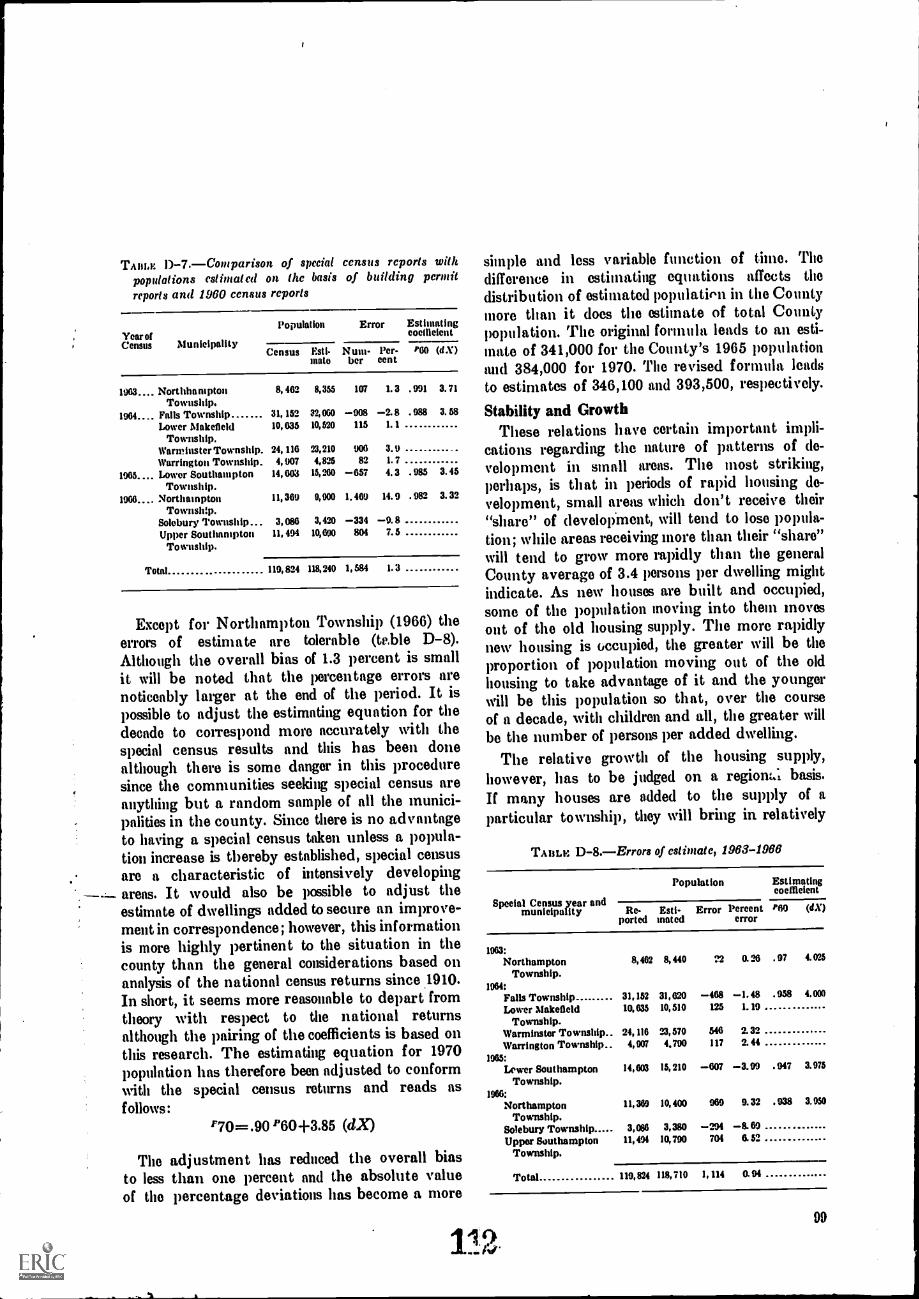
T D-7.Comparison of special census reports withpopulations estimated on the basis of building permitreports and 1960 census reports
Year ofCensus Municipality
Population Error Estimatingcoefficient
Census Esti- Num- Per- P60 (dX)mato her cent
Northhampton 8, 462 8,355 107 1. 3 . 991 3. 71
Township.1964.... Falls Township 31, 152 32,060 908 2. 8 . 988 3. 58
Lower Makefield 10,635 10,520 115 1. 1
Township.Warminster Township. 24, 116 23,210 006 3.9Warrington Township. 4, 907 4,825 82 1. 7
1965. Lower Southampton 14,603 15,260 657 4. 3 . 985 3. 45
Township.1966.... Northampton 11, 369 9,900 1. 469 14. 9 . 982 3. 32
Township.Solebury Township 3,086 3,420 334 9. 8Upper Southampton 11, 494 10,690 804 7. 5
Township.
Total 119,824 118,240 1, 584 I. 3
Except for Northampton Township (1966) theerrors of estimate are tolerable (te.ble D-8).Although the overall bias of 1.3 percent is smallit will be noted that the percentage errors arenoticeably larger at the end of the period. It ispossible to adjust the estimating equation for thedecade to correspond more accurately with thespecial census results and this has been donealthough there is some danger in this proceduresince the communities seeking special census areanything but a random sample of all the munici-palities in the county. Since there is no advantageto having a special census taken unless a popula-tion increase is thereby established, special censusare a characteristic of intensively developingareas. It would also be possible to adjust theestimate of dwellings added to secure an improve-ment in correspondence; however, this informationis more highly pertinent to the situation in thecounty than the general considerations based onanalysis of the national census returns since 1910.In short, it seems more reasonable to depart fromtheory with respect to the national returnsalthough the pturing of the coefficients is based onthis research. The estimating equation for 1970population has therefore been adjusted to conformwith the special census returns and reads asfollows:
F70= .90 P60+3.85 (dX)
The adjustment has reduced the overall biasto less than one percent and the absolute valueof the percentage deviations has become a more
simple and less variable function of time. Thedifference in estimating equations affects thedistribution of estimated population in the Countymore than it does the estimate of total Countypopulation. The original formula leads to an esti-mate of 341,000 for the County's 1965 populationand 384,000 for 1970. The revised formula leadsto estimates of 346,100 and 393,500, respectively.
Stability and GrowthThese relations have certain important impli-
cations regarding the nature of patterns of de-
velopment in small areas. The most striking,perhaps, is that in periods of rapid housing de-velopment, small areas which don't receive their"share" of development, will tend to lose popula-tion; while areas receiving more than their "share"will tend to grow more rapidly than the generalCounty average of 3.4 persons per dwelling mightindicate. As new houses are built and occupied,some of the population moving into them movesout of the old housing supply. The more rapidlynew housing is occupied, the greater will be theproportion of population moving out of the oldhousing to take advantage of it and the youngerwill be this population so that, over the courseof a decade, with children and all, the greater will
be the number of persons per added dwelling.
The relative growth of the housing supply,however, has to be judged on a regiont.; basis.
If many houses are added to the supply of aparticular township, they will bring in relatively
TA in. F: D-8.Errors of estimate, 1983-1988
Special Census year andmunicipality
Population Estimatingcoefficient
Re-ported
Esti-mated
Error Percenterror
P60 (CC)
1963:
Northampton 8, 462 8, 440 22 0. 26 . 97 4. 025
Township.1964:
Falls Township 31, 152 31,020 468 1. 48 . 958 4. 000
Lower Makefield 10, 635 10, 510 125 1. 19
Township.Warminster Township.. 24, 116 23,570 546 2. 32
Warrington Township.. 4, 907 4, 790 117 0 44
1965:Lcwer Sout hampton 14,603 15, 210 607 3. 99 . 947 3. 975
Township.1966:
Northampton 11, 369 10, 400 969 9.32 . 938 3. 950
Township.Solebury Township 3,086 3,380 294 8. 69
Upper Southampton 11, 494 10,790 704 6. 52
Township.
Total 119,824 118, 710 1, 114 0. 94
99
12
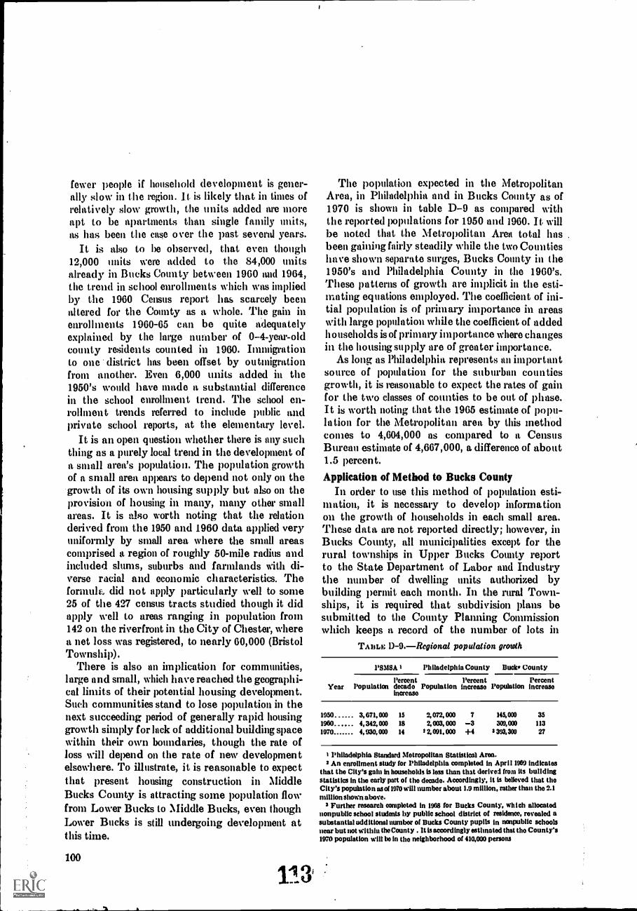
fewer people if household development is gener-ally slow in t he region. It is likely that in times ofrelatively slow growth, the units added are moreapt to be apartments than single family inths,as has been the case over the past several years.
It is also to be observed, that even though12,000 units were added to the 84,000 unitsalready in Bucks County between 1960 and 1964,the trend in school enrollments which was impliedby the 1960 Census report has scarcely beenaltered for the County as a whole. The gain inenrollments 1960-65 can be quite adequatelyexplained by the large number of 0-4-year-oldcounty residents counted in 1960. Immigrationto one district has been offset by outmigrationfrom another. Even 6,000 units added in the1950's would have made a substantial differencein the school enrollment trend. The school en-rollment trends referred to include public andprivate school reports, at the elementary level.
It is an open question whether there is any suchthing as a purely local trend in the development ofa small area's population. The population growthof a small area appears to depend not only on thegrowth of its own housing supply but also on theprovision of housing in many, many other smallareas. It is also worth noting that the relationderived from the 1950 and 1960 data applied veryuniformly by small area where the small areascomprised a region of roughly 50-mile radius andincluded slums, suburbs and farmlands with di-verse racial and economic characteristics. Theformulv, did not apply particularly well to some25 of the 427 census tracts studied though it didapply well to areas ranging in population from142 on the riverfront in the City of Chester, wherea net loss was registered, to nearly 60,000 (BristolTownship).
There is also an implication for communities,large and small, which have reached the geographi-cal limits of their potential housing development.Such communities stand to lose population in thenext succeeding period of generally rapid housinggrowth simply for lack of additional building spacewithin their own boundaries, though the rate ofloss will depend on the rate of new developmentelsewhere. To illustrate, it is reasonable to expectthat present housing construction in MiddleBucks County is attracting some population flowfrom Lower Bucks to Middle Bucks, even thoughLower Bucks is still undergoing development atthis time.
100
The population expected in the MetropolitanArea, in Philadelphia and in Bucks County as of1970 is shown in table D-9 as compared withthe reported populations for 1950 and 1960. It willbe noted that the Metropolitan Area total hasbeen gaining fairly steadily while the two Countieshave shown separate surges, Bucks County in the1950's and Philadelphia County in the 1960's.These patterns of growth are implicit in the esti-mating equations employed. The coefficient of ini-tial population is of primary importance in areaswith large population while the coefficient of addedhouseholds is of primary importance where changesin the housing supply are of greater importance.
As long as Philadelphia represents an importantsource of population for the suburban countiesgrowth, it is reasonable to expect the rates of gainfor the two classes of counties to be out of phase.It is worth noting that the 1965 estimate of popu-lation for the Metropolitan area by this methodcomes to 4,604,000 as compared to a CensusBureau estimate of 4,667,000, a difference of about1.5 percent.
Application of Method to Bucks CountyIn order to use this method of population esti-
mation, it is necessary to develop informationon the growth of households in each small area.These data are not reported directly; however, inBucks County, all municipalities except for therural townships in Upper Bucks County reportto the State Department of Labor and Industrythe number of dwelling units authorized bybuilding permit each month. In the rural Town-ships, it is required that subdivision plans besubmitted to the County Planning Conunissionwhich keeps a record of the number of lots in
TABLE D-9.Regional population growth
PSSISA Philadelphia County Buck, County
Percent Percent PercentYear Population decade Population increase Population increase
Increase
1950 3,671,000 15 2,072,003 7 145,000 35
1960 4,342,000 18 2,003,003 3 309,000 113
1970 4,930,000 14 2 2,091,003 +4 3 393,300 27
Philadelphia Standard Metropolitan Statistical Area.2 An enrollment study for Philadelphia completed in April 1969 indicates
that the City's gain in households is loss than that derived from its buildingstatistics in the early part of tho decade. Accordingly, it is believed that thoCity's population as of 1970 will number about 1.9 million, rather than tho 2.1million shown above.
3 Further research completed in 1968 for Ducks County, which allocatednonpublic school students by public school district of residence, revealed asubstantial additional number of Bucks County pupils in nonpublic schoolsnear but not within the County. . It is accordingly estimated that the County's1970 population will he in the neighborhood of 410,030 persons
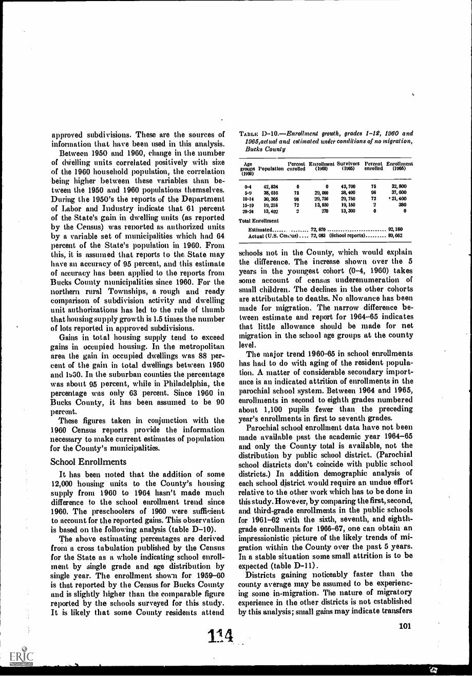
approved subdivisions. These are the sources ofinformation that have been used in this analysis.
Between 1950 and 1960, change in the numberof dWelling units correlated positively with sizeof the 1960 household population, the correlationbeing higher between these variables than be-tween the 1950 and 1960 populations themselves.During the 1950's the reports of the Departmentof Labor and Industry indicate that 61 percentof the State's gain in dwelling units (as reportedby the Census) was reported as authorized unitsby a variable set of municipalities which had 64percent of the State's population in 1960. Fromthis, it is assumed that reports to the, State mayhave an accuracy of 95 percent, and this estimateof accuracy has been applied to the reports fromBucks Comity municipalities since 1960. For thenorthern rural Townships, a rough and readycomparison of subdivision activity and dwellingunit authorizations has led to the rule of thumbthat housing supply growth is 1.5 times the numberof lots reported in approved subdivisions.
Gains in total housing supply tend to exceedgains in occupied housing. In the metropolitanarea the gain in occupied dwellings was 88 per-cent of the gain in total dwellings between 1950and 1b30. In the suburban counties the percentagewas about 95 percent, while in Philadelphia, thepercentage was only 63 percent. Since 1960 inBucks County, it has been assumed to be 90permit.
These figures taken in conjunction with the1960 Census reports provide the informationnecessary to make current estimates of populationfor the County's municipalities.
School EnrollmentsIt has been noted that the addition of some
12,000 housing units to the County's housingsupply from 1960 to 1964 hasn't made muchdifference to the school enrollment trend since1960. The preschoolers of 1960 were suffifientto account for the reported gains. This observationis based on the following analysis (table D-10).
The above estimating percentages are derivedfrom a cross tabulation published by the Censusfor the State as a whole indicating school enroll-ment by single grade and age distribution bysingle year. The enrollment shown for 1959-60is that reported by the Census for Bucks Countyand is slightly higher than the comparable figurereported by the schools surveyed for this study.It is likely that some County residents attend
114
TABLE 13-1O.Enrollment growth, grades 1-12, 1960 and1965,aclual and estimated under conditions of no migration,Bucks County
Ago Percent Enrollment, Survivors Percent Enrollmentgroups Population enrolled (1960) (1905) enrolled (1965)ONO)
0-4 .12, 834 0 0 43, 700 75 32, 800
5-9 38, 616 75 29, 000 38, 400 98 37, GOO
10-14 30, 365 98 29, 750 29, 750 72 / 21, 400
15-19 19, 218 72 13, 850 19, 150 2 380
20-24 13, 402 2 270 13, 300 0 0
Total Enrollment
Estimated 72, 870 92, 180
Actual (U.S. Celims).... 72, 083 (School reports) 89, 662
schools not in the County, which would explainthe difference. The increase shown over the 5years in the youngest cohort (0-4, 1960) takessonic account of census underenumeration ofsmall children. The declines in the other cohortsare attributable to deaths. No allowance has beenmade for migration. The narrow difference be-tween estimate and report for 1964-65 indicatesthat little allowance should be made for netmigration in the school age groups at the county
The major trend 1960-65 in school enrollmentshas had to do with aging of the resident popula-tion. A matter of considerable secondary import-ance is an indicated attrition of enrollments in theparochial school system. Between 1964 and 1965,enrollments in second to eighth grades numberedabout 1,100 pupils fewer than the precedingyear's enrollments in first to seventh grades.
Parochial school enrollment data have not beenmade available past the academic year 1964-65and only the County total is available, not thedistribution by public school district. (Parochialschool districts don't coincide with public schooldistricts.) In addition demographic analysis ofeach school district would require an undue effortrelative to the other work which has to be done inthis study. However, by comparing the first, second,and third-grade enrollments in the public schoolsfor 1961-62 with the sixth, seventh, and eighth-grade enrollinents for 1966-67, one can obtain animpressionistic picture of the likely trends of mi-gration within the County over the past 5 years.In a stable situation some small attrition is to beexpected (table D-11).
Districts gaining noticeably faster than thecounty average may be assumed to be experienc-ing some in-migration. The nature of migratoryexperience in the other districts is not establishedby this analysis; small gains may indicate transfers
101
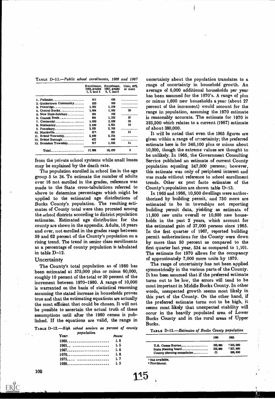
TABLE 1)-11.Public school enrollments, 1962 and 1967
Enrollment, Enrollment,1962, grades 1967, grades1, 2, and 3 0, 7, and 8
Gain, 10%or more
I. Palisades2. Quakertown Community
411
923
434
910
3. Pennridge 1, 201 1, 276
4. Central Bucks. 1, 004 1, 992 20
5. New llope-Solebury 201 193
0. Council Rock . 891 1, 222 37
7. Centennial. 1, 053 2,039 23
8. Neshaminy 2, 439 2, 821 10
9. Pennsbury. 2, 531 2, 703
10. Morrisville 21.'% 321 12
11. Bristol Township 3,490 3, 224
12. Bristol Borough 422 449
13. Bensalem Township 917 1, 035
Total 17,088 18, 079 9
from the private school systems while small lossesmay be explained by the death rate.
The population enrolled in school lies in the agegroup 5 to 34. To estimate the number of adultsover 16 not enrolled in the grades, reference wasmade to the State cross-tabulations referred toabove to determine percentages which might beapplied to the esthnated age distributions ofBucks County's population. The resulting esti-mates of County total were then prorated amongthe bchool districts according to district populationestimates. Estimated age distribution for thecounty are shown in the appendix. Adults, 16 yearsand over, not enrolled in the grades range between59 and 62 percent of the County's population on arising trend. The trend in senior class enrollmentsas a percentage of county population is tabulatedin table D-12.Uncertainty
The County's total population as of 1980 hasbeen estimated at 575,000 plus or minus 60,000,roughly 10 percent of the total or 30 percent of theincrement between 1970-1980. A range of 10,000is warranted on the basis of statistical reasoningassuming the stated increase in households provestrue and that the estimating equations are actuallythe most efficient that could be chosen. It will notbe possible to ascertain the actual truth of theseassumptions until after the 1980 census is pub-lished. If the equations are valid, the range inTABLE D-12.High school seniors as percent of county
populationYear: Percent
1960 1. 0
1965 1. 5
1967 1. 6
1970 1. 8
1975_ 1. 7
1980 1. 5
102
1i
uncertainty about the population translates to arange of uncertainty in household growth. Anaverage of 6,000 additional households per yearhas been assumed for the 1970's. A limp of plusor minus 1,600 new households a year (about 27percent of the increment) would account for therange in population, assuming the 1970 estimateis reasonably accurate. The estimate for 1970 is393,500 which relates to a current (1967) estimateof about 380,000.
It will be noted that even the 1965 figures aregiven within a range of uncertainty; the preferredestimate here is for 346,100 plus or minus about10,000, though the extreme values are thought tobe unlikely. In 1965, the Government ConsultingService published an estimate of current Countypopulation equaling 347,000 persons; however,this estimate was only of peripheral interest andwas made without reference to school enrollmenttrends. Other ex post facto estimates of theCounty's population are shown table D-13.
In 1965 and 1966, 10,500 dwellings were author-thorized by building permit, and 750 more areestimated to bs in townships not reportingbuilding permit data, yielding an estimate of11,800 new units overall or 10,600 new house-holds in the past 2 years, which account forthe estimated gain of 37,000 persons since 1965.In the first quarter of 1967, reported buildingpermit authorizations for the County were downby more than 50 percent as compared to thefirst quarter last year, 534 as compared to 1,101.The estimate for 1970 allows for the occupancyof approximately 7,000 more units by 1970.
The range of uncertainty has not been appliedsymmetrically in the various parts of the County.It has been assumed that if the preferred estimateturns out to be low, the errors will tend to bemost important in Middle Bucks County. In otherwords, unexpected growth seems most likely inthis part of the County. On the other hand, ifthe preferred estimate turns out to be high, itseems most likely that unexpected stability willoccur in the heavily populated area of LowerBucks County and in the rural areas of UpperBucks.
TABLE D-13.Eatimates of Bucks County population
1964 1965
U.S. Census Bureau 322,000 2 345,000
State planning board 323,800 2 327, 500
County planning commission 350, 850
I Not available.3 Provisional.
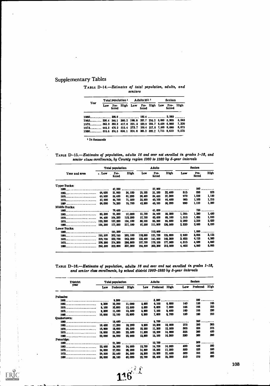
Supplementary TablesTABLE D-14.-Estima les of total population, adults, and
seniors
YearTotal population Adults 164- Seniors
Low Pre- High Low Pre- High Low Pre- Highferred tenni ferred
1960 308. 8 182.4 3, 2651965 330.4 348.1 360. 2 198. 8 207. 7 216. 2 4060 5,305 5,5451970 363.0 393.3 417.6 221. 5 239.9 254.7 6,420 6,860 7,3201975 445. 5 476. 2 515. 4 273. 7 295.4 217. 8 7,500 8,080 8,6751980 515.6 574.5 634.1 324.6 361.2 399.2 7,715 8,610 9,575
In thousands
TABLE D-15.-Estimates of population, adults 16 and over not enrolled in grades 1-12, andsenior class enrollments, by County region 1960 to 1980 by 5-year intervals
Year and area
Total population Adults Benton
.. Low Pre-ferred
High Low Pre-fared
II igh Low Pre-forted
High
U pper Bucks:1900 47, 200 27, 000 MO
1965 48, 030 51.900 M, BM 29,100 31, 100 32, 400 815 890 970
1970 49, 900 56, 400 61, 200 30,400 34, 400 37, 300 970 1, 050 1, 150
1975 57, 900 64, 700 71
34:40, 100 44, 400 985 1, 100 1, 215
1980 M. 000 74, 200 ,),,700 46, 100 50, 200 990 1, 110 1,200
Middle Bucks:1960 70, 400 41, 000 735
1965 ... 84 300 91, 500 97, 000 51, 700 54, 900 58, 200 1, 29b 1,380 1, 450
1974_ ... 94, 400 104, 200 113, 200 57, 700 63, 600 69, 100 1, 515 1, 685 1, 810
1975 129, 300 137, 200 154, 100 80, 100 85, 200 95, 500 Z MO Z 320 Z 620
1980 154, 300 173, 500 217, 100 97, 200 III, 800 136, 500 2, 320 2, 660 3, 310
Lower Bucks:1960 191, 200 113, 900 1,990
1965 195, 500 202, 700 200, 100 118, 000 121, 700 124 800 2, 950 3, 035 3, 125
1970 218 ZOO 233, POO 243, 200 133,400 141, 000 148.300 3. 935 4, 125 4, 300
1975 258, 300 274,300 288, 800 157,700 170, 100 177, 900 4, 315 4, 600 4, 840
1980 293, 300 322.800 337, 300 184, 600 203,300 212, 500 4, 405 4, 840 5, 065
TABLE D-16.-Estimates of population, adults 16 and over and not enrolled in grades 1-12,and senior class enrollments, by school district 1060-1980 by 5-year intervals
DistrictYear
Total population Adults Benton
Low Preferred High Low Preferred High Low Preferred High
Palisades:1960 9,300 5, 500 100
1965 9, 300 10,200 11, 000 5,600 6, 100 8, 600 140 150 165
1970 9, 100 10, 800 12, 500 5, 600 6, 600 7, 600 165 195 225
1975 9, 300 11, 400 13, 500 5, 800 7, 100 8, 400 180 195 230
1980 10, 000 12, 100 13, 800 6, 300 7, 600 8, 700 150 180 210
Quakertown:1960 19, 400 9, 700 240
1965 19, 400 13, 200 14 200 9, 800 10, 300 10, 900 275 290 305
1970 14 800 19, 000 20, 500 10, 200 11, 300 13, 500 305 335 375
1975 19, 000 21,300 23, 500 11, 800 13, 200 14, 600 325 300 400
1980 22, 000 24, 000 25, 900 13, 800 13, 100 14 300 330 360 390
Pennridge:1960 21, SOO 12, 700 300
1965 22, 900 24, WO 24, 900 13,700 14, 700 14, 900 400 450 500
1920 ... 24, 000 23,000 28, 200 14, 000 15, 500 17, 200 500 520 MO
1975 29, 500 33, 600 34, 500 19, 300 19, 800 21, 400 SOO 545 585
1980 34 000 39, 100 40, 000 22,700 23, 400 23, 200 510 570 000
103
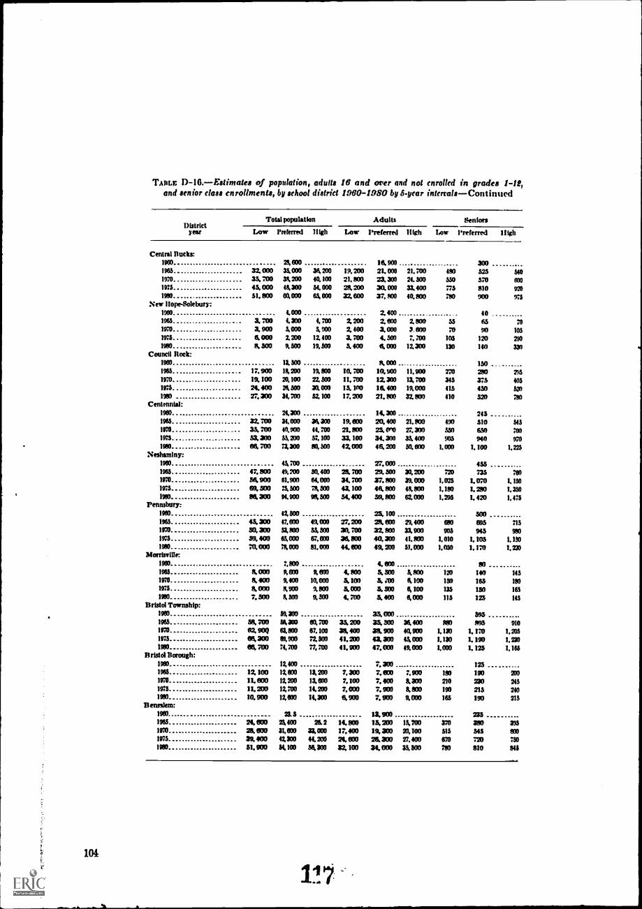
104
TABLE D-16.-Egitnates of population, adults 16 and over and not enrolled in grades 1-12,and senior class enrollments, by school district 1960-1980 by 6-year intervals-Continued
Districtyear
Total population Adults Seniors
Low Preferred High Low Preferred 1 I Igh Low Preferred High
Central Bucks:1960 23, 030 19. 900 300 ..196$ 32. 000 33, 000 34, 200 19, 200 23. 000 23, 700 480 523 3101970 35, :00 38 200 40, 100 21. 800 23. 300 24. 300 530 370 0001975 45. 000 43,300 54. 000 28, 200 30. 000 33, 400 773 810 9201980. 51, 800 00, 000 63, 000 32, 600 37, 800 40, 800 780 900 975
New 1 lope-Soleburr1900 4, 000 2. 400 401965 3.700 4,300 4.700 2.200 2. 000 2.800 ss 85 701970 9 900 3, 000 3, 900 2, 400 3, 000 3. 600 70 90 103193 6. 000 2, 200 12, 400 3. 700 4. 530 7, 700 103 120 2101980 9. 300 9, 500 19, 500 3. 400 0 000 13, 300 130 140 330
Council Rock:1903 13, 910 9 000 1501965 17, 900 18, 200 19, 000 10. 700 10 900 11, 900 270 280 2951970 19, 100 29, 100 22, 300 11, 700 IZ 300 13, 700 343 375 4031975 24, 400 24, 300 30, 000 13. 100 16. 400 19,000 415 430 5201990 27, 300 31, 700 33, 100 17. MO 21. POO 32, 800 410 320 780
Centennial:1960 24,300 14, 300 2431965 32, 1110 34. 000 34, 300 19 SOO 20, 400 21, 900 490 310 SO1970 35, 700 40.900 44, 700 21. 900 25, MO 27. 300 MO 630 7001975 53, 300 53, 200 57, 100 33, 100 34, 300 35, 400 903 940 9701900 60 700 mato 90, 300 42, COO 46, 200 30, MO 1. 000 1. 100 1, 223
Neshamlny:1900 43. 700 27. 000 455 ...1963 47, 900 49, 700 30, 400 20 700 29. 300 30, 200 720 73.8 no1970 34 SOO 61,900 64, 000 34. 700 37. 800 39, 000 1.023 L 070 1, 1501975. 69, 300 73, 500 73, 500 43, 100 44 900 45. 800 1.100 1. 280 1. 3S0190
rennsbury:80 300 91.903 98, 500 54, 400 59, 800 62, 000 1. as 3. 420 1. 47$
1900 42, 300 25. 100 3001965 45, 300 47, 600 49, 000 27, 200 29 9/0 29, 400 680 895 7151970 30 300 33, MO 33, 500 30, 700 32. 800 33, 90(1 003 943 9801975 59, 400 63, 000 67, 000 38, 900 40, 300 41, 930 1, 010 1, 103 1, 1501980 703, 000 78, 000 81, 000 44, 000 49, MO 31, 000 1, 050 1. 170 1, 220
Morrisville:1903 7,800 4, MO 931963 0 00o 9,00) 9, 030 4, 800 5, 500 3,10) 120 140 145tro 9. 400 9, 400 10, 000 5. 100 5. 100 4, 100 1311 165 1801975 9. 1300 9 900 9, 900 5, 000 5. 500 4, 100 13$ 150 1651900 7, 500 3,300 9, 300 4, 700 5. 400 4, 000 113 123 145
Bristol Township:1980. 59,300 33, 000 5951905. 30 700 54,300 01. ;00 33. 200 35. 300 34, 400 KO 993 9101270 82, 90Q 64.800 67, 100 38, 400 38, 900 40, 900 1, 130 L 170 1, 2031975 98, 300 04, 900 72,300 41, MO 43. 300 43, 000 1,130 L 190 1, 2301990 69. 700 74, loo 77, 700 41, 991 47, 000 49, 000 1, 000 I, 125 1. 165
Bristol Borough:1900 13. 400 7, 300 1231965 12, 100 13. 000 13, 200 7, 300 7, MO 7.900 180 190 2001970 IL GOO 13. 200 13, 600 7, 100 7, 400 8 300 210 230 2431973 11, 291 13.700 14, 200 7, 000 7, 900 8 800 190 213 2401980 10 900 12, 000 14.300 6, 900 7, 913 9, 0(10 165 190 215
Bensslem:1900 23. 5 13, 900 2351965 24. 800 23, 400 2& 2 14, 203 15. 200 13, 100 370 380 3931970 28, OM 33, 000 33, 000 17, 400 19. 300 20, 100 318 543 MO1975 39. 400 42,300 44, 200 24. 930 20 300 V, 400 070 720 no1900 53, 900 54. 100 50 300 32, 100 34, 000 33, 300 780 310 515
1
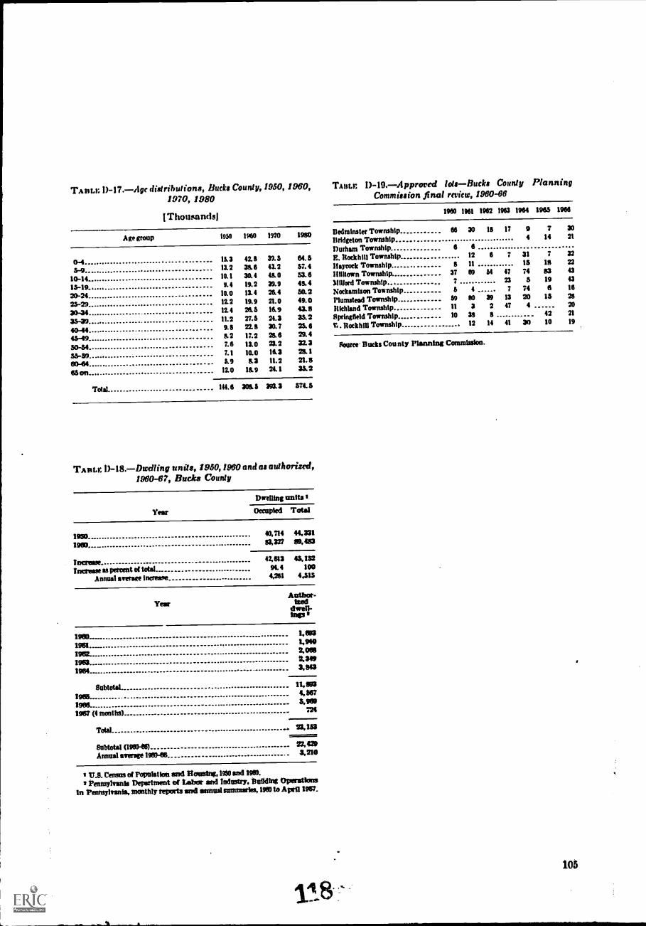
TABLE 1)-17.-Agc distributions, Bucks County, 1950, 1960, TABLE D-19.-Approred lots-Bucks County Planning
1970, 1980 Commission final review, 1960-66
(Thousands)
A018009 1930 1960 1970 1980
0-4 15.3 42.8 39. 5 64.5
5-9 13.2 35 6 43. 2 57. 4
10-14 10.1 30.4 450 33.6
15-19 I 4 19. 2 39.9 45 4
20-24 10.0 13.4 26.4 30.2
23-29 12. 2 19. 9 21 0 49.0
30-34 12.4 26 5 l& 9 43.8
35-29 11. 2 27.5 26.3 35. 2
40-44. 9. 8 22. 5 30. 7 23.6
45-49 5 2 17.2 28.6 29.4
50-54 7.6 110 23.2 32.3
5549 7. 1 10.0 16 3 25 1
80-64 5.9 53 11.2 21.8
6S on 12.0 15 9 W. 1 352
Total 144.6 305 3 393.3 574
TABLE 1)-18.-1)wdling units, 1950, /980 and as authorized,1960-67, Bucks County
Dwelling units
Year Occupied Total
1930 40,714 44,331
1960 83, 973 69.483
lacrosse 42,613 45,132
Increase in percent of total 94 4 100
Annual average increwee 4,261 4,315
YearAuthor-
Moddwell-ings I
1980 Lan1961 1,940
1982_ 2,063
1963 2. 349
ION I, 843
Subtotal 11,893
1985 4,867
19811 3,989
1967 (4 months) 724
Total *153
Subtotal (196)-68) 22, 429
Annual avenge 19E6496 3,210
II.S. Census of Population and Roush*, 1980 and 1960.Pennsylvatis Department of Labor and Industry. 13ti11din4 Operations
In Pennsylvania, monthly reports and animal sunclorties, 1960 to Mall 11967.
1960 1961 1962 1963 1964 1963 1966
Bedminster Township 66 30 18 1? 9 7 30
Bridgeton Township 4 14 21
Durham Township 6 6
E. Rock h Ill Township 12 6 7 31 7 32
Haycock Township 8 It 13 Is 22
11111lown Township 37 el SI 47 74 63 43
Milford Township 7 23 3 19 43
Nockamtson Township 6 4 7 74 6 16
Plumstead Township 59 60 39 13 20 13 28
Richland Township ll 3 2 47 4 20
Springfield Township 10 38 8 42 21
t . Itackhill Township 12 14 41 30 10 19
Source' Bucks Cou nty Planning Commission.
105
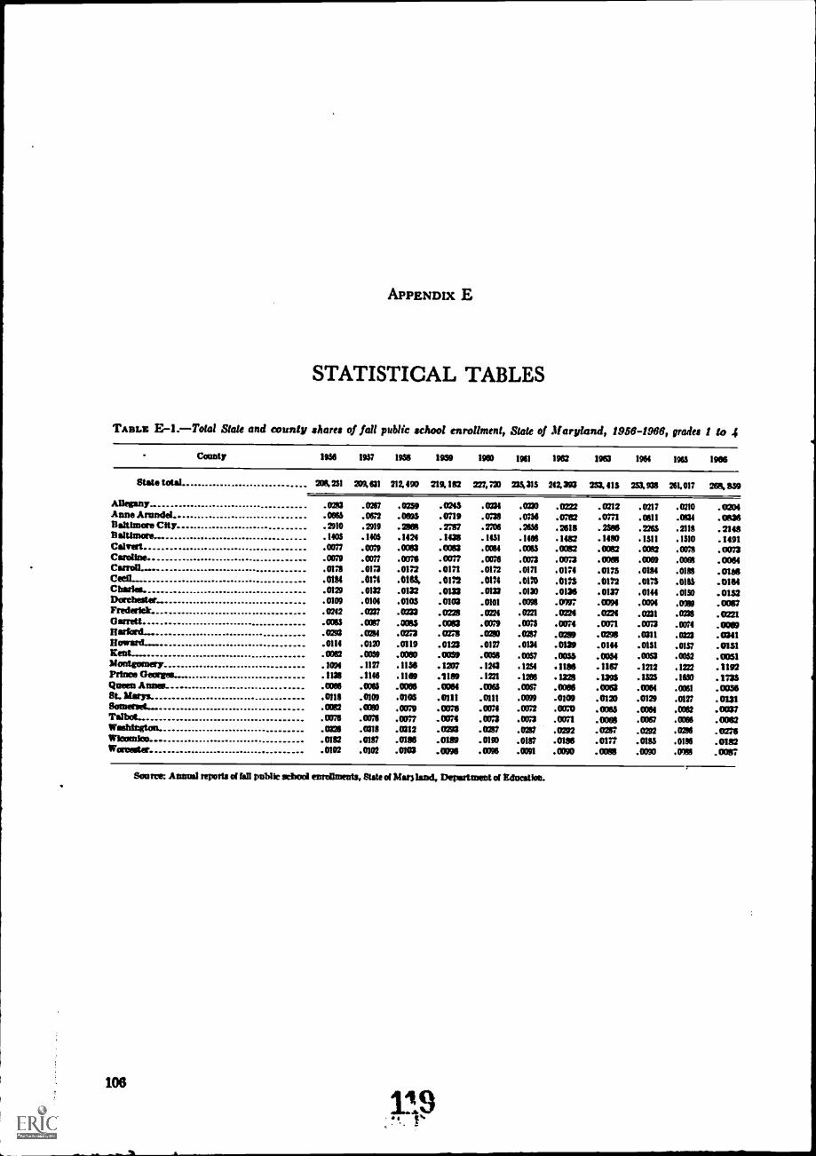
APPENDIX E
STATISTICAL TABLES
TABLE E-1.-Total Stale and county shares of fall public school enrollment, State of Maryland, 1958-1988, grades 1 to 4
County 1936 1957 1928 1939 1900 1961 1982 1963 1964 1965 1906
State total. 208.231 209,631 212.490 219.102 227,759 234313 242,393 233, 413 233,938 261.017 268. 659
Allegany 0283 .0267 .0239 .0243 .0234 .0230 .0222 .0212 .0217 .0210 .0204Anne Arundel. 0013 .0672 MOS .0719 .0138 .0754 0782 .0771 .0111 .0911 .0836Ealtimore City . 2910 . 2)19 . 2881 . 21717 .2706 . 2656 . 2618 , 2306 . 226S . 2119 . 2148lialtinsore... .1403 .1405 .1424 .1438 .1431 .1410 .1482 .1480 .1311 .1310 .1491Calvet .0071 .0019 .0083 .0083 .0084 .0063 .0082 .9% .0082 .0078 .0073Caroline .0079 .007; .0078 .0077 .0026 .0073 .0073 .0068 .0069 .0061 .0064Carroll. .0121 .0173 .0172 .0171 .0172 .0111 .0174 .0173 .0184 .0188 .0159Ceell____ .0184 .0171 .0103, .0112 .0171 .0124 .01/3 .0172 .0173 .0163 .0164Char1es. .0120 .0132 .0132 .0133 .0133 .0130 .0136 .0137 .0144 .0130 .0132Dorchester .0109 .0101 .0103 .0103 .0101 .0098 .0997 . WM .0091 .0189 .0087Frederick. .0242 .0227 .9% .0225 .0221 . 0221 .0224 .0224 .0231 .0238 .0221Garrett .0083 .0097 .0083 .0003 .0079 .0073 .0074 .0071 .0073 .0074 .0009itariord... .0293 .0284 .023 . OM .0200 .0247 .0289 .0298 .0311 .0323 .0341/toward.... .0114 .0120 .0119 .0123 .0127 .0134 .0139 .0144 .0131 .0137 .0131Kent_ .0062 .0039 .0000 .000 .0038 .0037 .0033 .0054 .0053 .0052 .0051Ifontgosun'y .1094 .1122 .1136 .1207 .1243 .1234 1186 .1187 .1212 .1222 .1192Prince Georges.... .1138 .1146 .1109 .1189 .1221 .1206 .1229 .1393 .1323 .1650 .1733Queen Anna! .0066 .0065 .0006 .0084 .0063 .0062 .0066 .0063 .0064 .0061 .0036St. Marys. .0119 .0109 .0103 .0111 .0111 .00)9 .0109 .0120 .0129 .0172 .0121Sonserset... .0082 .0090 .0079 .0016 .0024 .0072 .01720 .0063 .0064 .0062 .0037Tanya_ .0076 .0E6 0017 .0074 .0073 .0013 .0071 .9% .0067 .0088 .0062Washington. .03X .0118 .0312 .0293 .0217 .0292 .0292 .0217 .0292 .0280 . OMWiconfloo .0182 .0192 .0186 .0189 .0190 .0187 .0186 .0117 .0133 .0186 .0102Worcester. .0102 .0102 .0103 .0096 .0096 .0091 .0390 .0088 .0090 .0188 .0087
106
Salm Annusl reports of fall public school enrollMents, state of Man land, Department of Education.
119
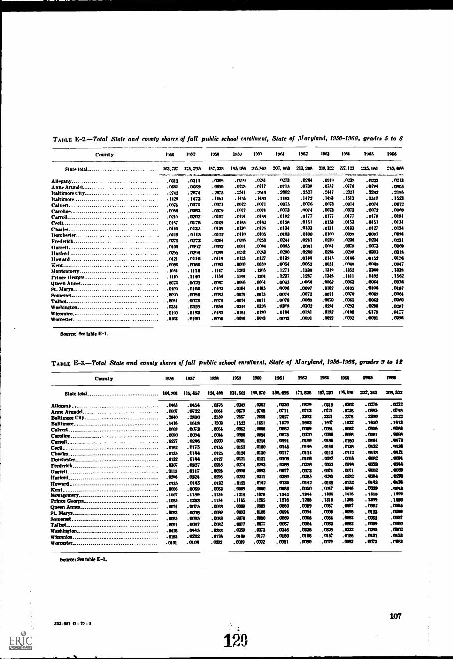
TABLE E-2.-Total State and county shares of fall public school enrollment, State of Maryland, 1958-1966, grades S to 8
Count y 1930 1997 192 1939 1900 2961 192 192 1964 1963 1966
State total .. 12, 73: 173. 213 197.331 143.92 203, $O 207. 2813 213. 22 219.322 227. 123 21. 961 243.62
Allegany. .213 . 0311 0306 . fee) .021 4273 . 0261 .0241 .029 .022 . 0213
A nne Arundel . o(Al . OW) . 0696 .0724 .0717 . 0713 . 0738 . 027 .0776 . 072 .CM33
Baltimore City . 7742 . 2674 . 2675 . 241 .264C, . 222 . 2527 . 2447 .221 . 2242 .2193
Baltimore . 142 . 1473 . 14s1 . 142 . 1480 . 1483 . 1472 . 1493 . 1313 . 1317 . 1323
Calvert .0073 . 0071 . 0071 . 0072 .0071 . 0073 . 0076 .0073 .0074 .0074 . 0012
Caroline 0211 . OW3 . 0079 . 0077 .0074 . 0073 . 0074 .012 .0073 .0072 .002Canon 0210 .202 .0197 .012 .012 .0182 .0177 .0177 .0177 .0178 .0191
Cecil .0117 .0176 .0160 .0163 .0162 .0138 .0151 .0153 .012 .0131 .0131
Charles . ono .0133 .0131 .0130 .0126 .0131 .0133 .0131 .012 .012 .0134
Ilorchest .0118 .0115 .0112 .0110 .0103 .0103 .0100 .0100 .000 .027 .002Frederkk .0273 .0773 . 0264 . .0233 . 0244 . 0241 . 0237 .0134 .0234 .0231
(I am4 t oleo . nna .0092 . 021 .0014 . 0013 .0081 .021 .271 .0073 .12911
Danced . 022 . 0294 . 0239 . 1 . 023 . 020 . 0 . 022 . 022 . 0335 . 031 s
Howard .0121 .0116 .0118 .0123 .0127 .0131 .0140 .0143 .0146 .0132 .0136
'gent 0066 . 0065 .002 . 002 . 0034 . 0032 .0031 .249 .11049 .0047
Montgomery . 1034 . 1114 . 1147 . 130 . 1203 . 1271 . 1330 . 1319 .1332 . 132 .1339
Prince ()earn9 .1110 .1140 .1154 .112 .1204 .1237 .1287 .1348 .1411 .1492 .1362
Queen A tines .023 .110113 .0067 .0366 .1064 . 005.S .102 .0062 .0003 .264 .0036
St. Marys .012 . 0105 . 0102 .0104 .0105 . 0796 . 0097 .0102 .0103 .0106 .0107
Somerset 22 .0104 .0182 .0024 .0073 .0074 . 0072 .0071 .270 .0001 .0164
Talbot .291 .0775 .0074 .0174 .0071 .0070 . 002 .0070 .063 .0062 .002Washington . . 0359 . 0334 .0341 .0326 . 0771 .11302 .021 .022 .0288 .022WIcornico .010 .0153 .0183 . elm .0190 .0194 .0111 .0182 .0110 .8179 .0177
Worcester . 0103 . 0100 .002 .026 .0073 . 002 . 01091 .0092 .1102 .0091 .1317101
Source: See tede E-1.
Tant.E E-3.-Total Stale and county shares of fall public school enrollment, State of Maryland, 1930-1988, grades 9 to It
County 1936 1957 1956 1993 1960 1961 1962 1963 1961 1963 192
State total 101, 801 115, 42 124, 416 131.502 140,20 136, 098 171, 838 197.20 191496 237,313 206.522
Allegany.. . 0163 . 024 . 0E6 . 249 .11352 . 032 . OM . 029 . OM _ 026 . 022Anne Arundel 062 .1E22 . 0564 . f29 . 0749 .1E11 .213 . 0211 .0725 .0693 .216Banknote City. . 2640 . 2830 . 2359 . 2357 . 2636 . 242 . 2333 . 2231 .2279 _zee .2122
Beltmore .1416 .1618 . 1503 .1522 .1631 .129 .1603 .127 .1622 .1630 . 213Calvert 203 .023 . MU . 0052 .22 . 0062 . 0059 . 0061 .0062 . 0036 . MaCaroline MO . 024 . 024 . 020 .214 . 023 . 0E0 .13086 . 0056 . 0061 .002Canoll 0227 . 0246 .17209 .0371 .0214 - 0191 . 0189 . 0136 .0190 .0161 .012Cecil 0162 . MI5 . 012 .0132 .0160 .0145 . M46 .0140 .012 .232 .0136
Charles 012 .0144 .0123 .0124 .0130 .0117 .0114 .0113 .0112 _0413 .0121
Doethester 0132 . 0144 . 0127 . 0121 .0121 . 0106 .0103 . 0037 . Me .0002 .1091
Prederick ONE . 0327 . 0285 .0E4 . 0293 . 029 . 0236 . 0332 . 0246 .023 . 024Garrett 0115 .0117 . 0099 . MN .023 . 027 . 0023 . OM .0E1 . 0062 -MOMilord 022 . 0324 . 022 . 032 .0311 . 0289 . 023 .0283 .0252 . 0264 .0213
1hnrard 0133 . 0145 .0132 .0125 .0142 . 0135 . 0142 . 01421 .0132 - 0143 . MNXent OM . 029 . 0053 . OM .0080 . 023 . 020 .021 . 0016 .0039 .023Montgomery .102 .1189 .1134 .1214 .1E6 .1342 .1344 MN .1416 .1453 .1499
Prtnce (kern; .1085 .1233 . 1134 .1163 .125 .1216 . 1289 .1319 .1365 .1399 .1480
Queen Armes 024 . 0075 .0068 . 0099 . 029 . 0060 . 029 . 0357 .11057 .0152 .026St. Mar's 0093 . 028 . 0099 023 .0106 . 0094 . OM .0095 .0096 . 012 . 002
Somerset 0085 . 0095 .023 . OM .0090 _0069 . 0066 .0064 .262 _0033 .6057
Talbot 0091 . 027 . 282 . 01122 . az . cos: .oces . 0063 .0052 - 0059 - 0090
Washington 0426 . 0445 . 032 . 029 . 0313 . 0346 .238 .0328 .0322 - 022 .0302
Wicamico 0195 .0202 .0176 .0103 .0117 . 0160 . 0138 . 01S/ . 0156 - 0131 . MaWorcester . 0101 . MOS . 0092 .000 . 2/2 . 0081 . 0090 . OM . 022 . 023 .22
Source: Eee table E-1.
353 -561 0.70.4
120
107'
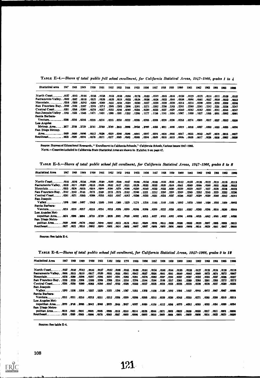
TABLE E-4.-Shares of total public fill school enrollment, for California Statistical Areas, 11047-1066, grades l to 4
Statistical area 194' 1943 1049 1950 1931 1952 1933 1954 1953 1936 1957 1938 1939 1960 1961 1962 1963 1964 196$ 1966
North Coast . .0137 .0145 .0144 .0156 .0136 .0133 .0158 .0161 .0176 .0161 .0149 .0145 .0144 .0134 .012) .0121 .0114 .0111 .0106 .0107Sacramento Valley. .0302 .0507 .0516 . 0621 .0526 .0620 .0324 .0333 .0526 . 0636 .0328 .0533 .0544 .0538 .0561 .(1561 .0537 . OSSO .0353 . OSS2Mountain .0316 .030) . 0Z12 0289 . 0269 . 0251 . 0248 . 0239 . 0230 0227 . 0220 . 0220 .0220 . 0214 . 0214 . 0203 . 0200 . 0203San Francisco Bay..2160 .2164 .22177 .2243 .2272 .2303 .2303 .2306 .2201 .2271 .2262 .2256 .2243 .2241 .2240 .2241 .2242 .2231 .2226 .2247Central Coast .0281 .0268 .0201 .0270 .0237 .0235 .11246 .0240 .0234 . OM9 .0233 . 0237 . .0240 . 0242 .0242 .0241 .0241 . (1244 .0247San Joaquin Valley .1915 .1333 .1546 . 1471 . 1431 .1363 .1301 .1232 . 1200 . 1177 1156 .1141 .1094 .1057 .1060 . .1033 .0391 .0202 .0991Santa Barbara-
Ventura .0203 .0216 .0216 .0219 .0214 .0215 .0210 .0222 .0205 .0206 .0208 .0220 .0238 .0251 .0274 .(001 .0517 . (037 .0352 .0339Los Angeles
Metrop. Area .3677 .3703 .3729 .3741 .3760 .3789 .3645 .3396 .3930 .3189 .4005 .4011 .4006 .4019 . 4016 .4(07 .4030 .4053 .40115 .4004San Diego Metrop.
Area ORO .0180 .006 .0612 .05011 .0559 .0940 .0686 .0011 .0927 .0304 .0616 .0646 .0647 .01656 .0643 .0127 .008 .0615 .0607Southeast 0623 .0589 .0594 .0576 .0671 .0.377 .0389 .0601 .0303 .0394 .0603 .0618 .0613 .0605 .0606 .0617 .0638 .0156 .0062 .0630
Source: Bureau of Educational Research." Enrollment in California Schooko.- Conferrals Moot., Various Issues 1947-1966.
Non..-Count les included in California State Statistical Areas ate shown in Ezhibit 9 on page 47.
TABLE E-6.-Shares of total public school fall enrollment, for California Statistical Areas, 1947-1966, grades 6 to 8
Statistical Area 1947 1943 1949 1930 1931 1932 1933 1954 1935 1936 1937 1958 1939 1900 1961 1962 1963 1964 1983 1966
North Coast .0144 .0166 .0136 .0168 .010) .0101 .0161 .0167 0166 .0136 .0148 .0144 .0144 .0142 .0133 .0126 .0122 .0118 .0116 .0113Sacramento Valley. .0313 .0511 .0530 .0316 . (613 .0632 .0627 .0331 . (ISA .0533 .0533 .0539 .0343 .0561 .0303 .0566 .0360 .0355 .0356 . OSS3Mountain 0115 .azn .1015 .UMM .02110 .0219 .0266 A0260 .0240 .0210 .0233 .0230 .029 .0271 .0221 .aza Jos .ans .0223San Frandsen Day. .2142 .2143 .2145 .2115 .2101 .2175 2173 2132 . 2221 .2212 .2250 .2255 .2249 .2245 .2232 .2245 .2223 .72/2 .2=16Central Coast 0281 .0271 .0265 .02011 .0215 .0231 .0247 .0242 .0236 .0225 .0231 .0234 .0237 .0234 .11217 .0231 .0239 .0240 .0242 .0244San lompiln
Valk, .1396 .1380 .1077 . 1543 .1301 .1444 .13M .1373 .1114 .1219 .1165 .1148 .1103 .1072 .1(170 .1050 .1033 .1016 .1009 .0993Santa Barbara-
Ventura 0214 .0219 .0217 .0213 .0214 .0213 .0203 .0272 .0206 .0208 .020) .0222 .0235 .0231 .0267 .0263 .0295 .0316 .0330 .0340Los Angeles Met-
ropolitan Area- .3674 .0396 .3694 .3719 .3759 .3326 .3901 .3150 .40ft2 .4015 .4027 .4010 .4002 .4001 .41118 . OM .4042 .4043 .4067 .4031San Diego Metro-
politan Ares .000 .0490 .0170 . ORO .0190 .0302 .0513 .0324 .0541 .0560 .0339 .0613 .006 .0636 .0633 .0633 .06117 .080S .0603 .0613Southeast 0527 .0621 .0610 .0002 .0208 .0001 .0614 .0033 .0007 .0607 .0008 .0009 .0601 .0800 .0606 .0614 .0620 .0641 .0647 .0643
Source: See table E-4.
TABLE E-6.-Shares of total public school fall enrollment, for California Statistical Areas, 1947-1966, grades 9 to 18
Statistical Area 190 1913 1949 1930 1931 1352 1953 129 1935 1936 1937 1938 1959 1960 1961 1962 1963 1964 19163 1966
North Coast 0137 .0140 .0142 .0151 .0157 .0162 .0108 .0163 .0106 .0161 .0134 .0146 .0144 .0135 .0133 .0127 .0123 .0124 .0120 .0118Sacramento Valley. 0198 .0315 .0510 .0617 .0620 .0531 .0334 .0341 .0562 .0537 .0014 .0541 .0541 .0650 .0562 .0569 .063 .0374 .0572 .0567Mountain .ans .ano Jos .0201 .0216 .0217 .021 .02a .own .026 .0260 .0249 .04 .0217 .0237 .0232 .0225 Jima .006 .0211,San Francisco Bay .2223 .2223 .2204 .2193 .230 .2313 .2214 .2210 .22011 .2194 .2194 .2198 .2217 .2261 .2M9 .2285 .2301 .2283 .2:12 .2772Central Coast 0254 0258 ONO . OX3 .0230 . 0247 .0243 .0213 .0233 .0227 .0225 .0224 .0225 .0220 .0225 .0226 .0226 .0220 .0230 .0335San ioaqnin
Valley .1330 .1326 .1354 . 1357 .1329 .1321 .1296 .1287 .1251 .1203 .1156 .1130 .1032 .1054 . 1027 .0995 .0912 .0967 .0967 .0960Santa Barbara-
Ventura .0211 .0211 .0210 .0213 .0211 .0212 .0313 .0209 .0206 .0203 .0212 .0220 Arno .0243 .0235 .0211 .0335 .0299 .0310 .0315Los Angeles Met-
ropolitan Area... .1g9 . rag .3966 .3942 .3916 . .3949 .3957 .4007 .4069 .4119 .4112 .4096 .44770 .4052 .4055 .4053 .4034 .4000 .4054San Diego Metro-
politan Ares 0518 .0481 .0191 .0501 .0503 .0018 .0513 .0510 .0514 .0328 .0544 .0571 .0003 .11622 .0639 .0633 .0617 .0611 . .0601Southeast 0554 0509 .0565 .0506 .0518 .0563 .0587 .003 .0396 .0600 .0610 .0609 .0608 .0601 .0600 .0606 .0614 .0523 .0623 .06X1
Source: See table IA
108
121
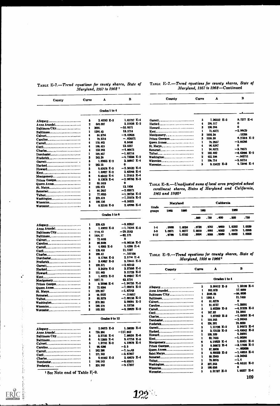
TAnt.r. E-7.-Trcnd equations for county shares, State of TAnt.t: F.-7.-Trend equations for county shares, State ofMaryland, 1957 to 19621 Maryland, 1957 to 1962-Continued
County Curve A
Grades 1 to 4
AlleganyAnne ArundelBaltimore CityBaltimoreCalvedCarolineCarrollCecilCharlesDorchesterFrederickGarrettIlarford
521
1
4
1
4
4
4
1
352
3.40243 E-3646007
3001.
13M.4354.9754
79.5714
170.463
165419133.94$
10555724135
1.09653 E-225115
1.61797 E-42.51458 E-2
-55 857113.5714
-3 4263$- 9285716.5456
13.5257-4.86471-1.85714-4.73336 E-2
3.50647 E-4o
!toward IS 9.02176 Z-3 -2.30132 13.-4
Kent 5 139027 E-2 2. 82916 E-4
Montgomery 5 503422 E4 1.21913 E-4
Prince Geoltell 5 9.12616 E-4 -2.05793 E-3Queen Anne% 2 56.1419 oSt. Marys 4 103.9:3 13.1358
Somerset. 1 64.2557 -103311
Talbot 2 77.9333 -1.20734 E-2Washington 3 229-43 -1.21078 E-2Wicomico 4 192.156 -O. 50321
Worcester 5 9-32145 E-3 2.49900 E-4
Grades 5 to 8
Allegany 1 325429 -8.92557Anne Arundel 5 1.41072 E-3 -1.74244 E-3Baltimore City I 2748. 43 -29.2143Baltimore 4 1405.1: -62. 171
Calvert 3 714453 0
Caroline 3 Se. 5468 96130 E-2
Canon .. 3 4.6303 E-3 1.4200 E-4
Cecil 4 121455 11.1137
Charles 3 15542 -.101550
Dorchester 5 117494 E-3 2.57oo E-4
Frederick 5 3.49607 E-3 0.19443 E-3
Garrett 1 KRIM 2.82143
Harked 3 3.31379 E-3 3.37956 E-5
Howard 2 111.462 3.11123 E-2
Kent.. S 1. 4ons E-2 & 99347 E-4
Montgomery 1 1017.71 415714
Prince Georges S 9.20056 E4 -1.91135 F.-3
Queen Annes 3 71 93M -7.05974 F.-2
St. Marys. 1 101557 -1.82143Somerset 3 910132 -.114017
Talbot 3 81 5273 -1.01156 E-2Washington 2 319.185 3.09M1 E-2WIcomIco 4 150.179 9.15158
Worcester 3 103.335 -6.23629 E-2
Grades 9 to 12
Allegany 5 104075 E-3 1.56039 F.-4
Anne Anmdel 4 736.364 -117. 042Baltimore City 6 157151 E4 7.88024 1-6Baltimore 6 & 12593 E-4 5 47716 E-5
Calvert S 137741 E-2 4.19876 E-4
Caroline 1 96 4286 -3.5Carroll 1 242.256 -7. 5.43Cecil 1 171.143 -3.5357Charles 5 & 91952 E-3 2.49679 E-4
Dorchester 1 146143 -6.03571Frederick. 1 324.143 -9.17837
I See note end of Table
County Curve A
Garrett!Wordthnnird
54
3
7.36532 E-3298 117136 244
8.7277 E-4oo
Kent 1 71.5571 -2.96429Montgomery. 3 1016311 .15208
Prince Georges 3 115538 627316 E-2
Queen Annes 1 752137 -2.81256St. Marys . 4 96 5= oSomerset I 94.8571 -13371Talbot 2 102.402 -6.63585 E-2Washington 2 432.196 -.013711Wkornico 1 191714 -5.85714
Worcester 5 9.1M22 E-3 4.73456 E-4
Tmn.E E-8.-Unadjuatcd sums of local arca projected schoolenrollment shares, States of Maryland and California,1965 and 19801
tiradeMaryland California
1985 1980 1965 1980groups
. 500 .750 . 400 . 500 . 150
1-4 .9988 LOOM .935 .932 .9809 1.0282 1.0039
64 1.0011 Lam 1.0019 .9964 .9503 .9970 1.0098
9-12 .9768 1.0102 .9994 .9991 .9509 1.0003 1.0055
TAnt: E-9.-Trend cquations for county shares, Slate ofMaryland, 1956 to 19661
County Curve A
Grades 1 to 4
Allegany 3 3.30412 E-3 1.33199 E-4
Anne Arundel 1 842. g3 17.9909
Balthnore City. . 1 3106.25 -84.0528
Baltimore 1 1393.4 11.1453
Calved 4 51.6279 0
Caroline 1 51.4P27 -1.83031
Candi 3 3.92M9 E-3 -4.31225 E-5
Cecil 4 167.82 14.5644
Charles 5 7.97032 E-3 -1.09092 E-4
Dorchester 1 110.545 -2.01345
Frederick 4 224.201 138039
Garrett 5 1.11128 E-2 2.94972 E-1
Harked 3 3.12123 E-3 -5 49042 F.-.1
Howard 1 101109 4.39091
Kent 1 517455 -1.06364
Montgmnery 6 5146= E4 1.05131 Z-4
Prince Georges 3 9-50872 13-4 -3.17405 13-5
Queen Annes 1 St 8308 -.663636
Saint Marys 5 9.80033 E-3 -1.44618 13-4
Somerset 1 852543 -134545Talbot I It 5818 -1.4Washington 3 327.545 -644151 E-2Wkomko 3 186.055 o
Wonestet. 5 9-51737 E-3 1.95327 K-4
109
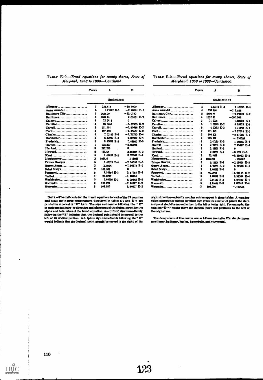
TAnt.r. E-9.-Trend equations for county shares, State of TAntx E-9.-Trend equations for county shares, Stale ofMaryland, 1956 to 1966-Continued Maryland, 1956 to 1986-Continued
Curve A Curve A
Grades 3 to 8 Oracles 9 to 12
Allegany 1 334.415 -10. 6909 Allegany 5 2.07312 E4 1.46388 E-4Anne Arundel 5 I. 49542 E4 -2. 26151 E-3 Anne Arundel 4 7319M -115646Baltimore City 1 252129 -53. 0152 Baltimore City 2 MI 44 -2.19373 E-2Baltimore 3 1435 44 2.08151 E-2 Baltimore 4 1637.19 -207.03Calvert 4 nom 0 Calvert 3 71.2238 7.50016 E4Caroline 3 M. 6236 -6.37305 E-2 Caroline 1.02160 E-2 518925 E4Carroll 3 211.991 -7 80688 E-2 Carroll 4.0:612 E-3 1.3482 E4Cecil 3 187.313 -9. 48557 E-2 Cecil 2 171.393 -2.27018 E4Charles 6 7 :2185 F.4 -529293 E-4 Charles 3 140.33 -15 5M73 E4Dorchester 3 11.329C6 E 2.03862 E-4 Dorchester 2 14536 -.0307154Frederick 5 3.53632 E4 7 441932 E-S Frederick IS 3. C1019 E4 1.05265 E-4Genet 1 109.327 -2. WW1 Hasten 2.89501 E-3 7.23867 E-4Harrold 3 257.293 o Harford 3.14421 E4Howard 2 111.65 3.07696 E-2 Howard 7.63601 E4 -6.999 E-3Kent 3 1.41492 E-2 6.70587 E4 Kent 2 73. NM -S. 45912 E-2Montgomery 3 1031.6 .11503.5 Ihmtgomery 3 1012.03 .15637Prince Georges 3 0.42074 E-4 -291537 E-3 Prince Georges 9.15604 E-4 -2.01624 E4Queen Annes 3 73.205 -7.36578 E-2 Queen Annes 1.25054 3.81553 E4Saint Marys 2 103. MS o Saint Marys L09233 E-2Somerset 5 1.10494 B-2 3. 675 E4 Someryet . 2 97. ?)14 -3.24145 E-2Talbot 1 61637 -1.76384 Talbot L 00491 E-2 6.143205 E4Washington 3 2.83658 E4 529462 E4 Washington 3 2.21342 E4 1.08162 E-4Wicomko 3 LW 372 -2.14817 E-2 Wicomico 3. MOM E-3 1.67245 E4Worcester 3 103 OST S. 54027 1:-2 Worcester 3 108.215 -.129456
Notx.-The coefficients for the trend equations kr nth of the 24 countiesand three gre !e group combinations displayed in taMes E.: and E-9 ateprinted in exponent or "E" form. The sign and number following the "E"in each case indicates the direction and placeMent of the decimal point fat thealpha and beta values of the trend equation. A- (r-tnts) sign immediatelyfollowing the "E" indicates that the decimal point should be moved to thelen of its original position. A+ (Plus) sign immediately following ihe"E"would indicate that the decimal point should be moved to the right of its
110
edgiest position-tactually no plus entries appear in these tables. A numbetvalue following the minus (or plus) sign gives the number of places the defl-mat point should be moved either to the left or to the tight. For example, thenotation" E-4" means move the decimal point four positions to the left ofthe original me.
The designations of the cur-es me as follows (see table 27): simple linearcurvilinear, log linear, log log, hyperbolic, and exponential.
123
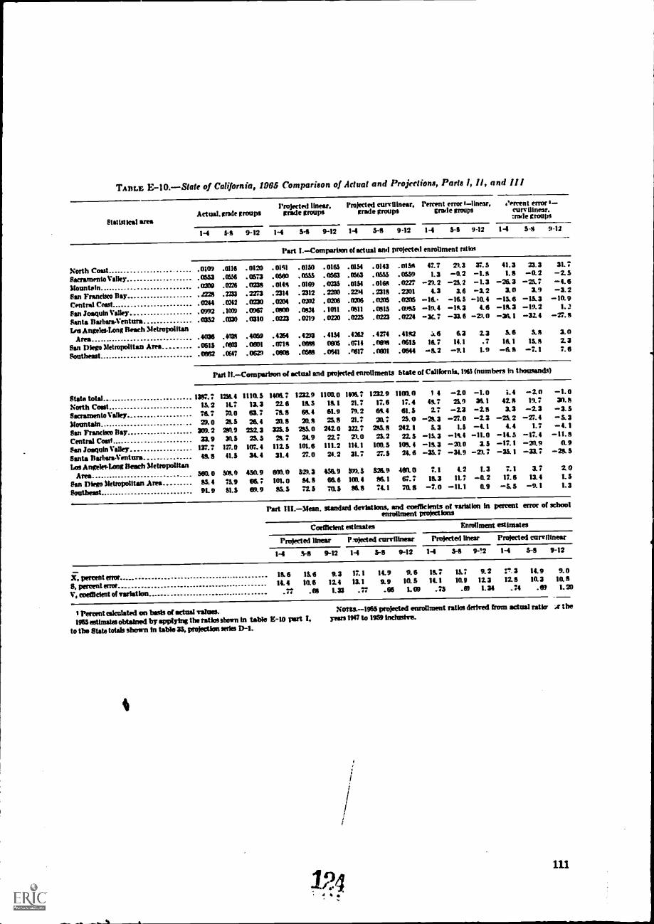
TAM.E E-10.-State of California, 1965 Comparison of Actual and Projections, Parts I, II, and II I
Statistical area641411. trade groups
1-4 5-6 9-12
North Cosst .0103 .0116 .0120
Sacramento Valley 0553 .0556 .0573
stountsin 0209 .0226 .0236
San Francisco Day 2225 .2253 .2213
Centnd Coast 0244 .0142 . 0220
San Joaquin Valley 0992 .103) .036:Santa flarbara-Ventura 0352 .0330 .0310
Les Angeles-Long Desch MetropolitanAres .4036 .4034 .4059
San Diego Metmpolitan Ares 0615 . .0601
Southeast .0662 .0647 .0621
Projected linear, Projected curvilinear. Percent error 1-11near. eercent error 1-grade groups Made groups grode groups curvilinesr.
:rade groups
1-4 5-6 9-12 1-4 3-5 9-12 1-4 5-5 9-12 1-4 5-8 9-12
Part 1.-Comparison of actual and projected enrollment ratios
.0141 .0150 .0165 .0154 .0143 .0156 41.7 29.3 37.5 41.3 25.3 31. 7
.0560 .0555 .0561 .0563 .0555 .0559 1.3 -0.2 -I.S I. 8 -0.2 -2. S
.0146 .0109 .0235 .0134 .0166 .0227 -29.2 - 23 2 -1.3 -26.3 -25.7 -t 6
.2314 .2312 . 2203 .224 . 2316 .2201 4.3 3.6 -3.2 10 19 -3. 2
. 0201 . 0202 . 0206 . (1206 . ams .0315 -1& -16. 5 -10. 4 -15. 6 -13. 3 -10.9
. ONO . OS24 . 1011 .0611 .0615 .0955 -19.4 -13.3 4.6 -13.3 -19.2 I. 1
.0223 .0219 0220 .0225 .0223 .0224 -347 -33.6 -21.0 -36.1 -32.4 -27.5
.4264 .4293 . 4154 .4262 .4114 .4162 :$.6 6.3 2.3 3.6 & 3.0
.0718 .0666 0005 .0714 .0015 .0615 16.7 14.1 .7 l& 1 15.6 2. 3
.0606 .096 .0541 .0617 .0001 .0644 -& 2 -9.1 1.9 -6. -7.1 7.6
Part 11.-Compertion of actual and projected enrollments State of California, 1965 (numbers in thousands)
State total lac.: 12564 1110.5 1408.7 1232.9 1100.0 140&: 1232.9 1100.0 1 4 -2.0 -1.0
Notth Coast 13.2 14.: 11 3 22.6 13.5 l& 1 21.7 17.6 17.4 4t 7 25.9 36.1
Samatnento Valley 76.: 70.0 617 789 63. 4 61.9 19.2 641. 4 61.5 2.7 -2.3 -IRSlormtaln 23.0 2&5 2& 4 Ma 20.1 25.11 21.7 20.7 25.0 -263 -27.0 -2.3
San Eranclsco flay 331 2 260.9 252.3 213. 5 265.0 242.0 222.: Mt 5 242. 1 5.3 1.5 -4.1
Central Coast 33.9 XS 25.5 2t7 24.9 22.7 71.0 25.2 22.5 -1&3 -PIA -11.0
San Joequin Valley I37.7 127.0 107.4 112.5 101.6 111.2 114.1 100.5 101 4 -163 -20.0 3.5
Santa Darbara-Ventnra 49. 5 41.5 34. 4 31.4 27.0 24.2 31. 7 27.5 21. 6 -3& 7 -3t 9 -29. 7
Los Antelei-Long Heath MetropolitanArea WO. 0 503.0 450. 9 eva. 0 521. 3 438 9 309. 3 VS& 9 461 0 :A 4. 2 1. 3
San Diego Metropolitan Area 63 4 75.9 436.7 101.0 64.5 66.6 100.4 86.1 67.7 163 11.7 -0.2
Southeast 91. 9 81.3 fn. 9 65.3 :2.3 70.3 96.5 74.1 70.9 -7.0 -11.1 0.9
14 -2.0 -1.042.8 19.1 at 813 -2.3 -3.5
-2.5.2 -27.4 -5.34.4 1.7 -4. 1
-14.5 -17.4 -11.5-11.1 -21.9 0.9- 3& 1
7. 1 3.1 2 011.6 13.4 1.5
- & 3 -9.1 1.3
Part 1/1.-Mean. standard deviationa, and coefficients of variation In percent error of schoolenrollment projections
Coefficient estimates Enrollment estbnates
Projected linear Pujected curvilinear Projected linear Projected curvilinear
14 6-8 9-12 1-4 5-0 9-12 1-4 31 9-!2 1-4 5-8 9-12
1T, percent enot 166 15.8 9.3 17.1 14.9 9.6 18: 131 9.2 11". 3 14.9 9.0
6. percent error 14.4 10.6 12.4 13.1 9.9 10.5 14.1 10.9 12.3 12.8 10.3 MS
V, coefficient of variatkrn .66 1.33 .77 .66 1.09 .75 .69 1.34 .:4 .03 1.20
1 Percent twkolated on basis of actual values.1265 estimates obtained by applying the laths shown In table E-10 part I.,
to tbe State totals shown in table 35, projection series 1)-1.
Notts.-1965 projected enrollment ratios delved from actual ratio' r tbeyears 1847 to 1959 inclusive.
124ill
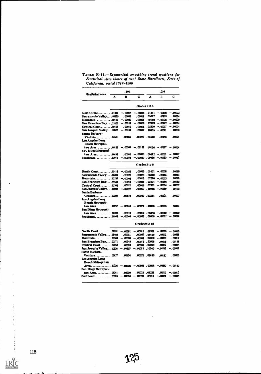
TAHLE E-11.-Erponenlial smoothing trend equations forStatistical Area shares of total State Enrollment, State ofCalifornia, period 1947-1960
Statistical area.500 .750
A B C A
Grades 1 to 4
North Coast .01342 -.00091 -.00016 .01341 -.00108 -.00023Sacramento Valley... .00570 .00E3 .00011 .03377 .00119 .00034Mountain .02149 -.03039 .00001 .07140 -.00020San Francisco Bay.. .22406 -.00244 -.00058 .22393 -.00242 -.00034Central Coast .024t9 .00012 . 00005 .02329 -.00004San Joaquin Valley .10656 -.00131 .03E2 .10965 -.00071 .00093Santa Barbara-
Ventura 02531 .0E66 .00027 .02330 .00156 .00021
Los Angeles-LongBeach Metropoli-tan Ares . 40149 -. 00309 -. 00157 56 -. E217 -. 00024
Sal Diego Metropoli-tan Ares 00496 .09091 -.000E .06472 -.03021 -.00077
Southeast .03079 -.00078 -.00030 .00056 -.00067
Grades 5 to 8
North Coast 01416 -.0E24 .00003 .01421 -.00008 .00010Sacramento Valley... .05803 .00120 .00020 .05610 . 00143 . OEMMountain . 10209 - . 00001 .00016 .02290 -.03003 .00015
Son Francisco Bay- .72513 .00044 -.00031 .22491 -.00166 -.03142Central Coast ... .02368 .00021 .00009 .02361 -.00004 -.00007San Joaquin Valley.. .10998 -.00197 .00057 .10916 -.00119 .00103Santa Barbara-
Ventura .02509 .00170 .00029 .02511 .00171 .00077Los Angeles-Long
Beach Metropoli-tan Ana 40E7 -.00146 -.00073 .40036 -.00005 .00014
San Diego Metropoli-tan Area .06392 .00110 -.00019 .06363 -.EEO -.EEO
Southeast . .0E03 -.ODOM -.00009 .00E0 -.03052 -.00014
Grades 9 to 12
North Coast. .01351 -.09381 -.00E1 .01334 -.0000 -.00015Sacramento Valley._ . EMS . 00051 .00007 .0510 .0E1093 .03031Mountain .02363 -.00096 -.03003 .0=0 -.00059 .03E2San Francisco Bay_ .2E71 .013411 .00E5 .23308 . M493 . OEMCentral Coast .02250 .00010 .00006 .02250 .0E07 .00006San Joaquin Valley.. .10535 -.00393 -.11110I3 .10640 -.00362 -.03339Sante Ba.-bara-
Ventura 02427 .00131 .00022 .02430 .00142 .00E6Los Angeles-Long
Beach MetroplitattArea 40736 -.00236 -.00102 .40096 -.0E62 -. 00102
San Diego Metropoli-tan Area 06241 .00290 . OWE .06223 .03212 -.0E17
Southeast 00016 -.00E3 -. 0=0 .06011 -.EOM -.0E38
112
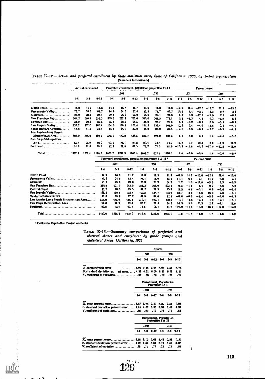
Tsntc E-12.-Adua/ and projcckd enrollment by State statistical area, State of California, 1905, by 4-4-4 organization[Numbers in thousands)
Actual enrollment Projrcted enrollment, population projection D-1 1 Percent error
14 5.5
.500 .730 .500 .750
9-12 1-4 5-6 9 12 1-4 5-8 9-12 1-4 5-5 9-12 1-4 5-5 9-12
North Coast. 15.2 14.7 13.3 14.1 168 11.7 13.2 12.8 11.3 -7.2 11.4 -12.5 -12.7 21.1 -15.0Sacramento Valley 76.7 700 es.; ste 74.5 62.4 87.8 76.7 63.2 10.6 6.4 -2.0 14.5 9.6 2.5Mountain MO 765 25.4 29.4 217 23.0 26.2 29.1 24.8 1.3 0.8 -12.9 -9.9 2.1 -6 2San Francisco hay ar 2 280.9 252.3 309.5 7:7.3 263.6 310. 0 261.5 773. 1 (L 1 -1.3 4.5 0.3 -5.8 6. 3Central Coast 33.9 315 23.5 33.6 30.5 25.5 310 28.7 23 3 & 1 -0.2 -0.1 0.5 -5.8 -0.9San Joaquin Valley 137.7 121.f 107.4 156.6 130.1 102.4 159.5 136.4 103.0 12.3 2.4 -4.6 1511 7.4 -41Santa llarbara-Vcntura 48.8 41.5 34.4 45.4 36.7 32.2 44.6 310 32.8 -7.0 -6.8 -64 -8.7 -62 -4.5Los Angeles-Lon! (leach
Metrormlitan Area 560. 0 SOIL 0 450.9 583 7 482. 8 433.5 367.7 496.0 478. 3 -I. 1 -5.0 -3.4 1.4 -2.4 -5.0San Dir.to Metropolitan
Arts 63. 4 73.9 66.7 97.2 81.7 80.3 87.4 73.4 74.7 13.8 7.7 20.3 2.3 -3.3 11.9Southeast 91.9 815 01.9 62.4 71.9 61.5 76.2 71.5 61.4 -10.3 -11.8 -9.2 -12.0 -12.2 -11.9
Total . 1387.7 1236.4 1110.5 1406.7 1232.9 1100.0 1406.7 1222.9 1100.0 1.4 -2.0 -0.9 1.4 -2.0 -0.9Projected enrollment, population projection I & 1 Percent error
.500 .730 .367 .730
1-4 5-5 9-12 1-4 5-6 9-12 1-4 5-8 9-12 1-4 35 9-12
North Coast 14.2 16 11.7 113 12.8 11.3 -6.8 14.7 -12.6 -12.4 21.4 -16.0Sacramento Valley QS. 2 74.6 62.4 PS. 1 76.9 65.2 11.1 6.6 -2.1 14.9 9.8 2.4Mountain . 21.5 218 23.0 26.3 212 24.7 I. 1.0 -12.9 -9.5 2.3 -63San Francbco Day 310.8 277.9 263.5 311.3 265.0 713.1 0.5 -1.1 4.4 0.7 -5.6 5.2Central Coast 3&7 315 ZS. 5 36 2 XS 25.3 5.5 0.4 -0.1 0.9 -5.6 -1.0San Joaquin Valley 155.2 131 4 102.4 160.2 136.7 192.9 11 7 2.6 -4.6 16.3 7.6 -4.1Santa flarbara-Ventura_ 45.6 368 32.2 44.8 39.0 32.8 -6.6 -6.6 -6.4 -5.3 -6.0 -4.8Los Anteles-Long 'leach Metropolitan Area 556.0 40.9 433. 4 510.1 497.1 478.1 -0.7 -4.8 -3.4 1.8 -2.1 -5.1San Dim) Metropolitan Ares 97.6 519 803 87.7 73.5 74.7 14.3 10 013 2.7 -3.1 11.9Southemt 82.8 72.0 63.5 16.6 71.7 61.6 -16.0 -11.6 -9.2 -16.7 -12.0 --110
Total 1412.6 1235.6 1099.7 1412.6 12356 1035.7 18 -18 -1.0 1.8 -1.8 -1.0
1 California Population Projection Series
TAW: 1..-13.-Sumnutry comparisons of projected andobserved shares and enrollment by grade groups andStatistical Arras, California, 1005
Shares
.500
14 5-8 9-12 1-4 5-8 9-12
IV, mean percent error 6.91 7.16 7.26 8.29 7.53 6.73S. standard deviation p, nt error 4 SS 4.71 6.05 6.51 6.73 4.51V, coellident of variation 06 .06 .83 .19 .89 .M
Enrollment, PopulationProjection 1)-1
.500 .750
1-4 5-8 9-12 1-4 5-8 9-12
X, mean percent error 6.87 5.05 7.59 6.3. 7.59 1.06S. standard deviation petcent error 4 63 4.52 5.85 634 3.42 4.34V. coefficient of variation .68 .80 .77 .16 .71 .61
Enrollment, PopulationProjection I & II
.500 .750
1-4 5-8 9-12 1-4 5-8 9-12
X, man percent error 6 95 5.72 7.61 8.43 7.56 2.178, standard deviation percent error 4.72 4.52 5.84 614 5.31 3.88V, coefficient of variation .68 .79 .17 .13 .73 .55
118
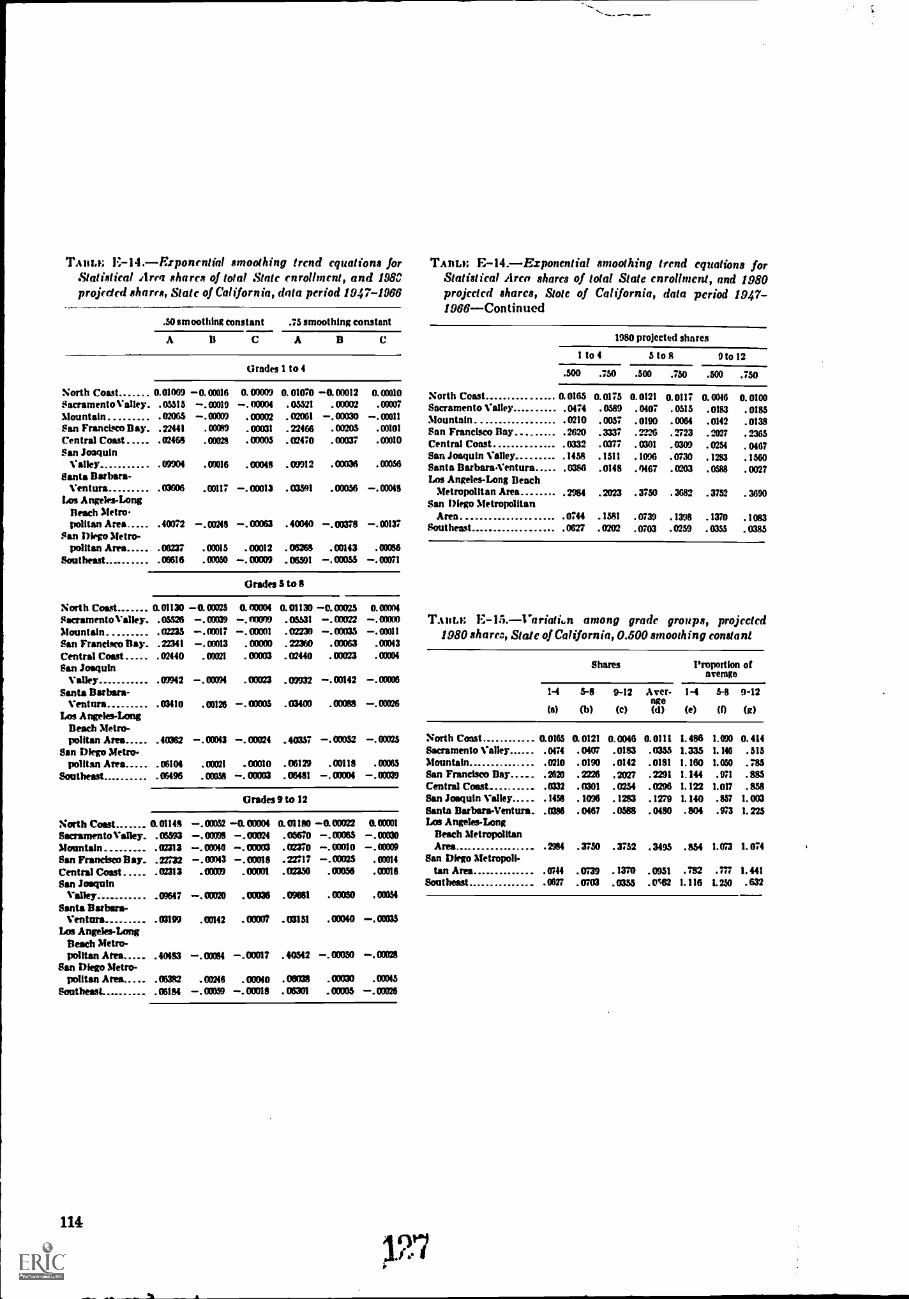
TAIII.I; E-14.-Erponential smoothing trend equations forStatistkal Area shares of total State enrolhnent, and 198Cprojeded shares, Stale of C'alifornia, data period 1947-1968
.W smoothing constant .75 smoothing constant
A II C A
Grades 1 to 4
North Coast 0. 0100) -0.00016 0.00009 0. 01070 -0.00012 0.00010Sacramento Valley. .05315 -.00019 -. 00004 .03321 .00002 .00007Mountain 02065 -.00009 .00002 . W061 -.00030 -.00011San Francisco Bay. .22441 . 00389 .00031 .22466 .00205 .00101
Central Coast 02468 .00028 .00005 .02470 .00037 .00010
San JoaquinValley. . 09904 .00016 .00048 .W912 .00036 .00056
Santa Barbara-Ventura 03W6 .00117 -.00013 .03301 .00056 -.00048
Los Angeles-LongBeach Metro.politan Area .40072 -.0O248 -.03063 .40040 -.00378 -.00137
San Diego Metro-politan Area .06237 .00015 .00012 .0626S .00143 .00386
Southeast 06616 .00050 -.00009 .06591 -.00055 -.00071
Grades 5 to 8
North Coast 0.01130 -0.00023 0. MOM 0.01130 -0.01025 0. 00004
SacramentoVaIley. .03526 -.00039 .05531 -.00022 -.00000Mountain 02235 -.00017 -.00001 . 02230 -. 00035 -.00011San Francisco Bay. .22341 -. 06013 . 00000 .22360 .00063 .W043Central Coast 02440 .00021 . 00003 . 02440 . 00(123 .00004
San JoaquinVs WY .09942 -.000X .00023 .09932 -.0142 -.00008
Santa Barbara-Ventura MO .00126 -.00005 .03400 .00M8 -.00026
Los Angeles-LongBeach Metro-politan Area .40362 -.00043 -.0004 40357 -.00)52 -.00725
San Diego Metro-politan Area .06101 .00021 .00010 .06129 O118 .00063
Southeast. 06496 . -.0(1003 .06481 -.00004 -.00039
Grades 9 to 12
North Coast 0.0114S -.WW2 -0.00004 0.01180 -0.00022 0.00001
Sacramento Valley. .05393 -.WM -.00024 . 05670 -. 00063 -. 00030Mountain .. .02313 -. 00040 -. 00033 . 02M0 - 00010 - 00009San Francisco nay. .2232 -.MG -.00018 .zar; -.03025 .W014
Central Coast 02313 . 00009 . own .02330 00056 03016
San JoaquinValiey .09647 -. 00020 . 00036 . 09681 . 00050 . 000M
Santa 8arbara-Ventura .03199 .00142 .00007 .03151 .00010 -.0003$
Los Angeles-LongBeach Metro-politan Area . 40483 -. 00084 -. 001317 . 40342 -. 00W0 0/028
San Diego Metro-politan .06382 .00246 .000W .00038 . .00045
Southeast. . 06184 -. 00059 -. 00018 . 06301 . 00005 -. 00M6
114
V.
TABLE E-14.-Exponential smoothing trend equations forStatistical Area shares of total Stale enrollment, and 1980projected shares, State of California, data period 1947-1988-Contin ued
1980 projected shares
1 to 4 5 to 8 Oto 12
.500 .750 .500 .750 .500 .750
North Coast .. 0. 0165 0. 0175 0. 0121 0. 0117 0. 0046 0. 0100Sacramento Valley 0474 .0589 .0407 . 0515 .0183 . 0185Mountain . 0210 .0057 .0190 .0064 .0142 .0138San Francisco Bay .. .2620 .3337 .2226 . 2723 .2365Central Coast . 033" .0377 . 0301 .0309 .0254 . 0467San Joaquin Valley 1458 .1511 .1096 .0730 .1283 .1560Santa Ilarbara-Ventura .0386 .0148 .0467 .0203 .0588 .0027Los Angeles-Long Beach
Metropolitan Area 2984 .2023 .3750 . 3682 .3752 . 3690San Diego Metropolitan
Area 0744 .1581 . 0739 .1398 .1370 . 1083Southeast 0627 .0202 .0703 .0259 .0355 . 0385
TABLE E-15.-l'ariatLn among grade groups, projected1980 share; State of California, 0.500 smoothing constant
Shares Proportion ofaverage
1-4
(a)
5-8
(b)
9-12
(c)
Aver-age(d)
1-4
(e)
5-8
(I)
9-12
(R)
North Comt 0.0165 0.0121 0.0046 0.0111 1. 486 1.090 0. 414Sacramento Valley . .0474 .0407 .0183 .0355 1.335 1.146 .515Mountain .0210 . 0190 .0142 .0181 1. 160 1.050 .785San Francisco Bay .2620 .2226 .2027 .2291 1.144 .971 .885Central Coast .0332 .0301 .0254 .0296 1. 122 1.017 .858San Joaquin Valley_ .1458 . 1096 . 1283 .1279 1. 140 .857 1.003Santa Barbara-Ventura_ .0386 .0467 .0938 .0480 . 801 .973 1. 22SLos Angeles-Long
Beach MetropolitanArea .2984 .3730 .3752 .3495 .854 1.073 1.074
Ban Men Metr090litan Area .0744 .0739 . 1370 .0951 .782 .777 I. 441
Southeast .0627 .0703 .0355 .062 1.116 1.250 .632
APPENDIX F
THE MULTIPLE REGRESSION APPROACH
The idea behind this approach is simple enough;we seek out a number of factors in an effort toexplain changes in the proportion of the State'senrollment found in a given county. For example,one county might have a continuously higher birthrate and thus have a higher proportion of childrenenrolled in public school. Accordingly, this ap-proach was tried for Maryland. Unfortunately, itdid not provide projections more accurate thanthose obtained from the procedures discussed inchapters 5 to 8. Furthermore, the amount ofpreparation involved in using it is very consid-erable. Nevertheless, with the thought that itmight prove to be useful in some other States, weare presenting it here. Only empirical testing be-yond the scope of this study will determine howuseful it may turn out to be.
The multiple regression equation or "cohort-ratio" is derived from the observed relationshipof the changes in a number of different sympto-matic data series to changes in shares of totalschool enrollment accounted for by a local politicalunit. In the case of the Maryland tests, therewere three dependent variables for each of the24 counties representing the three gradegroupsthe "4-4-4" organization of enrollment.Each dependent or "Y" variable in the regressionequation represents the ratio of the county's shareof the total State enrollment in a given year; forexample, .1956 to its share in the following year,1957. Thus for each grade-grouping, and eachcounty in the experiments, there was a total of10 dependent variables representing cohort-ratiosfor the years 1956 to 1966. The independent or"X" variables are expressed in the same way.The "X" variables in the experiments were:
Variable:Resident Births by CountyResident Deaths by CountyRetail Sales by CountyNumber of Households by CountyEffective Buying Income by CountyResident Income Tax Returns filed by County_Registered Private Vehicles by CountyResident Ineurne Paid by County
Symbol
XIX2X3X4X3X6X2Xl
A total of 75 multiple regression equations werederived from the basic data. Each of the 24counties had three multiple regression equationsfitted to the basic dataone for each of the threegrade groupings. In addition, all the data pointsfor all the counties were used to derive threeseparate multiple regression equations for theState of Maryland. The object of the 25th set ofestimating equations was to test the forecastingefficiency of the "State" versus the individuallytailored county forecasting enrollment ratios. Asan example of the application of the technique,the results of the regression analyses are shown intables F-1 to F-8 and cover the years 1956 to1962, inclusive, for Calvert County, Md.
For making projections of school enrollment, itis only necessary to project each of the independentvariables to the target date. Then, utilizing themultiple regression equation constants, thecounty's share of the total State enrollment isultimately obtained.
Specific Steps in the Approach
There are a total of seven steps in the use ofthe multiple-regression or cohort-ratio approach.
Step 1. The compilation and computation of theshares of State annual series on school enrollment,the dependent or "Y" variables, and the inde-pendent or "X" variables described next.
*Pt
128
115
Step 2. Computation of the cohort ratios of thedependent and independent variables.
Step 3. Development of multiple regressionestimating relationships of the cohort ratio ofcounty share of total State school enrollment,using the annual series of data for the independentor "X" variables developed in Step 2. This wasaccomplished for the three grade groupings foreach county and for the "State."
Step 4. Fitting statistical trend functions to thesignificant independent or "X" variables derivedin Step 3.
Step 5. Extrapolation of trend functions ofsignificant independent or "X" variables derivedin Stop 3.
Step 6. Solution of multiple regression equationderived in Step 3, using projected values forsignificant independent or "X" variables derivedin Step 5.
Step 7. Application of projected county enroll-ment shares of total State enrollment to inde-pendently derived total State enrollmentprojections.
Data Base Development and Description
In order to implement the school enrollmentratio, cohort-ratio multiple regression approachfor Maryland, several historical series on demo-graphic and economic changes in the counties hadto be developed. The historical period covered inthe tests was from 1955 to 1966.
The several demographic and economic historicalseries were derived from a variety of public andprivate published and unpublished sources.
County school enrollment ratios for gradegroups 1-4, 5-8 and 9-12 were derived fromStatistics on Enrollment and Number of Schools,Public and Nonpublic, State of Maryland, pub-lished annually by the Division of Research andDevelopment, Maryland State Department ofEducation.
Resident births and deaths by county in Mary-land, covering the period from 1955 to 1966, werederived from unpublished vital statistics seriesprovided the project and prepared by the Divi-sion of Biostatistics, Department of Health, Stateof Maryland.
Statistics on the number of privately registeredautomobiles by county for the period 1955 to 1966were obtained from the Director of Public In-formation, Department of Motor Vehicles, Stateof Maryland. The tallies for ea& county repre-
116
sented the total number of privately owned motorvehicles registered as of April 30 in each year.
Historical series on the number of households,volume of retail sales, and effeiltive buying incomeper household for counties fin Maryland, werederived from data publishld annually in the"Survey of Buying Power". published by SalesManagement magazine about the .second week inJune. The data published cover each State, countyand State of Maryland Statistical Areas (SMSA).
Data on the annual number of resident incometax returns filed by county in Maryland, as wellas the residential income tax take per county,were derived from Resident Income Tax Returnsfor the Year , published by the Comptrollerof the Treasury, Income Tax Division, State ofMaryland. The summary report on the volume ofresident income tax returns filed by county cov-ered the period from 1959 to 1965. To fill in thegaps, trend lines were fitted to the available datafor each county and estimates derived for the'years 1956 to 1958 and 1966.
Two additional historical series were consideredoriginally for the analysis, but were dropped sub-sequently because of significant lacunae in thedata. U.S. Bureau of the Census, Construction Re-ports, Building Permits, Series C-40, containsmonthly and annual summaries of building per-mits let by permit-issuing places in the UnitedStates. Out of the 24 counties in Maryland, only15 were effectively covered under the Censusseries. Collection of building permit data fromthe counties was considered impractical and timeconsuming. U.S. Bureau of -the Census, CountyBusiness Patterns, contains fairly detailed data onthe industrial affiliation of the labor force of eachcounty in the United States and would haveproved of some assistance in the Maryland tests.However, the series has been published continu-ously and annually only since 1964. Prior to thattime, the series was published every 3 years. Acheck with the State of Maryland, Bureau ofEmployment Security, revealed that continuoushistorical data on labor force composition bycounty was available only for the counties com-prising the Baltimore SMSA and for Alleganyand Washington, the latter designated as eco-nomically distressed areas in the AppalachiaProgram of the U.S. Department of Commerce,Economic Development Administration. At somefuture date, the U.S. Census County BusinessPatterns labor force estimates by county shouldbe considered as a substitute or additional hide-
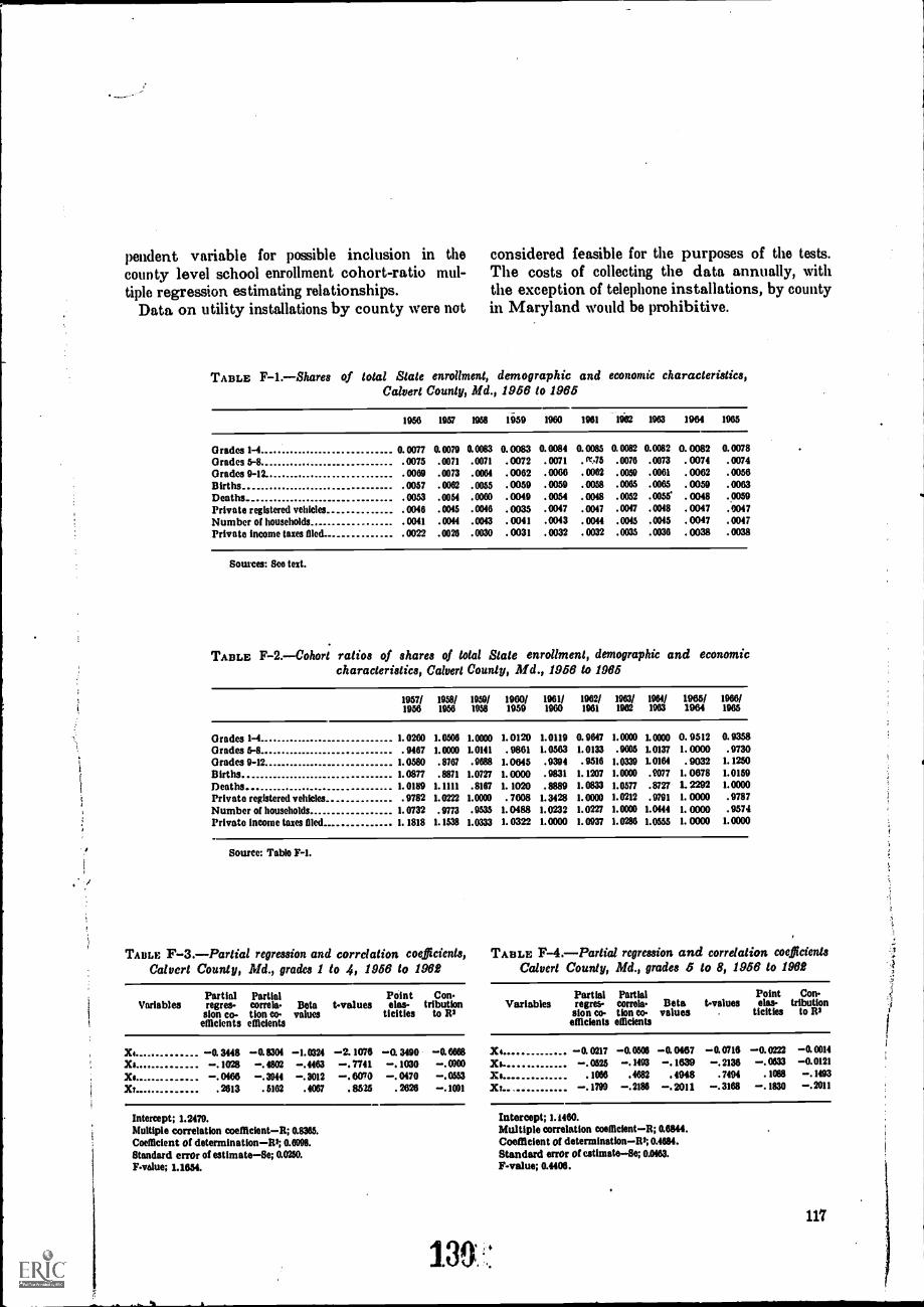
pendent variable for possible inclusion in thecounty level school enrollment cohort-ratio mul-tiple regression estimating relationships.
Data on utility installations by county were not
considered feasible for the purposes of the tests.The costs of collecting the data annually, withthe exception of telephone installations, by countyin Maryland would be prohibitive.
TABLE F-1.-Shares of total State enrollment, demographic and economic characteristics,Calvert County, Md., 1956 to 1965
1956 1957 mu 1659 1960 1961 1952 1963 1964 1965
Grades 1-4 0.0077 0.0079 0.0083 0. 0083 0.0084 0.0085 0.0082 0.0082 0. 0082 0.0078Grades 5-8 .0075 .0071 .0071 . 0072 .0071 . m75 .0076 .0073 . 0074 .0074Grades 9-12. .0069 .0073 .0064 .0062 .0060 .0062 .0050 .0061 .0062 .0056Births .0057 .0062 .0055 .0059 .0059 .0058 .0065 .0065 . 0059 .0063Deaths .0053 .0054 .0060 .0049 .0054 .0048 .0052 .0055 .0048 .0059Private registered vehicles 0046 .0045 .0046 .0035 .0047 .0047 .0047 .0048 . 0047 .9047Number of households 0041 .0044 .0043 .0041 .0043 .0044 .0045 .0045 .0047 .0047Private income taxes filed .0022 .0026 .0030 .0031 .0032 .0032 .0035 .0036 .0038 .0038
Sources: See text.
TABLE F-2.-Cohort ratios of shares of total State enrollment, demographic and economiccharacteristics, Calvert County, Md., 1956 to 1965
1957/1956
1958/1956
1959/1058
1960/1959
1961/1960
1962/1961
1963/1962
1964/1963
1965/1964
1966/1965
Grades 1-4 1.0260 1.0506 1.0000 1.0120 1.0119 0.9647 1.0000 1.0000 0.9512 0.9358Grades 5-8 9467 1.0000 1.0141 .9861 1.0563 1.0133 .9605 1.0137 1.0000 .9730Grades 9-12 1.0580 .8767 .9688 1.0645 .9394 .9516 1.0339 1.0164 .9032 1.1250
Births 1.0877 .8871 1.0727 1.0000 .9831 1.1207 1.0000 .2077 1.0678 1.0159
Deaths 1.0189 1.1111 .8167 1.1020 .8889 1.0833 1.0577 .8727 1. 2292 1.0000
Private registered vehicles 9782 1.0222 1.0000 .7608 1.3428 1.0000 1.0212 .9791 1.0000 .9787Number of households 1.0732 .9773 .9335 1.0488 1.0232 1.0227 1.0000 1.0444 1.0000 .9574Private income taxes filed 1.1818 1.1538 1.0333 1.0322 1.0000 1.0937 1.0286 1.0555 1.0000 1.0000
Source: Table F-1.
TABLE F-3.-Partial regression and correlation coefficients, TABLE F-4.-Partial regression and correlation coefficientsCalvert County, Md., grades 1 to 4, 1956 to 1968 Calvert County, Md., grades 5 to 8, 1956 to 1968
Partial PartialVariables regres- correla- Beta t-values
sion co- tion co valuesefficients efficients
Point Con.elas- tribution
ticities to It3
Partial Partial Point Con-Variables regres- correla- Beta t-values elu tribution
Mon co. tion co- values McKie" to It3efficient' efficient'
X -0.3448 -0.8304 -10324 -2.1076 -0.3490 -0.6668 X1 -0.0217 -0.0506 -0.0467 -0.0716 -0.0222 -0.0014
Xs -.1028 - 4802 - 4463 - 7741 -.1030 -.MOO Xs. - 0525 -.1493 -.1639 -.2136 -.033 -0.0121
Xe - 0466 - 3944 - 3012 - 6070 - 0470 -.0553 Xe .1066 .4682 .4948 .7494 .1088 -.1493Xi 2613 .5162 4067 8525 2828 -.1091 -.1799 -.218 -. 2011 -.3168 -.1830 -.2011
Intercept; 1.2479.Multiple correlation coeflicient-R; 0.8365.Coefficient of determination-Rs; 0.6998.Standard error of estimate-8e; 0.0250.F-value; 1.1654.
Intercept; 1.1460.Multiple correlation Coefficient-R; 0.6844.Coefficient of determinatlon-Rs; 0.4684.Standard error of estimate-Se; 0.0463.F-value; 0.4406.
117
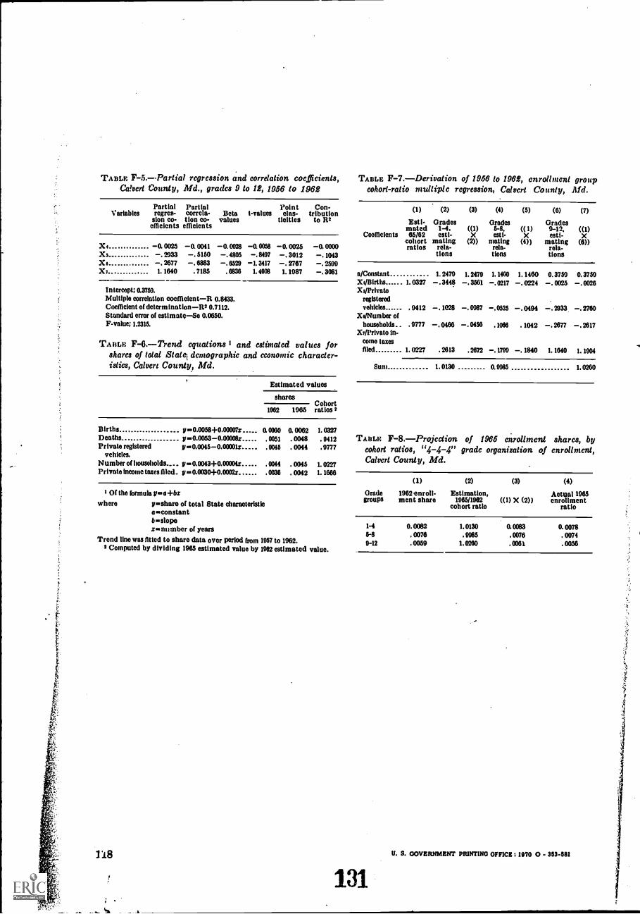
TABLE F-5.Partial regression and correlation coefficients,Ca!vert County, Md., grades 9 to 12, 1956 to 1962
Partial Partial Point Con-Variables regres- correla- Beta t-values etas- tribution
sion co- tion co- values ticities to R2efficients efficients
X. -0.0025 -0. 0041 -0.0028 -0.0058 -0. 0025 -0.0000Xs - 2933 -. 5150 -. 4805 -. 8497 -. 3012 -. 1043X - 2677 -. 6883 -. 6529 -I. 3417 -. 2767 -. 2599Xs . 1. 1640 . 7185 . 6836 1. 4608 1. 1987 -. 3081
Intercept; 0.3759.Multiple correlation coefficient-R 0.8433.Coefficient of determination-EA 0.7112.Standard error of estimate-Se 0.0650.F-value; 1.2315.
TABLE F-6.-Trend equations 1 and estimated values forshares of total Stateq demographic and economic character-istics, Calvert County, Md.
Estimated values
sharesCohortratios 21962 1965
Births y =0.0058+0.00007s 0. 0080 0.0052 1. 0327Deaths y =0.0053-0.00008x . 0351 .0048 . 9412Private registered y =0.0045 -0.0000Is
vehicles.. 0045 . 0044 .9777
Number of households._ y =0.0043+0.00004x . 0044 . 0045 1. 0227Private income taxes filed. y=0.0030+0.0002: . 0036 . 0042 1. 1686
I Of the formula y +bswhere y=sharo of total State characteristic
a =constantb =slopez number of years
Trend line was fitted to share data over period from 1957 to 1962.2 Computed by dividing 1965 estimated value by 1962 estimated value.
118
TABLE F-7.-Derivalion of 1956 to 1962, enrollment groupcohort-ratio ntultiple regression, Calvert County, Md.
(1) (2)
Esti- Gradesmated 1-4,
Coefficients 65/02 esti-cohort matingratios rela-
tions
(3) (4)
Grades((I) 5-8,)( est I-
(2)) matingrela-tions
(5) (6) (7)
Oracles(( 1) 9-12, ((1)X esti- )(
(4)) mating (1)))rela-tions
a/Constant 1. 2479 I. 2479 1. 1460 1. 1460 0.3759 O. 3759X./Births...... I. 0327 -. 3448 -. 3561 -. 0217 -. 0224 -. 0025 -.0026Xs/Privato
registeredvehicles .9412 -.1028 -.0987 -.0525 -.0494 -.2933 -.2750
X./Number ofhouseholds_ .9777 -.0466 -.0456 .1066 . 1042 -. 2677 -. 2617
Xs/Privato in-come taxesfiled I. 0227 . 2613 . 2672 -. 1799 -. 1840 1. 1640 1. 1904
Sum 1.0130 0.9985 1.0250
TABLE F-8.-Projection of 1965 enrollment shares, bycohort ratios, "4-4-4" grade organization of enrollment,Calvert County, Md.
Gradegroups
(1)
1962 onroll-ment share
(2) (3)
Estimation,1965/1982
cohort ratio
(4)
Actual 1965((I) )( (2)) enrollment
ratio
1-4
tr89-12
0.0082. 0076.0059
1.0130.9985
1.0260
0.0083.0076.0051
0. 0078. 0074. 0050
131
U. S. GOVERNMENT PRINTING OFFICE : 1970 0 - 353-581
Related Documents