07 April 2010 Denver, CO OPTIMIZING DEVELOPMENT STRATEGIES TO INCREASE RESERVES IN UNCONVENTIONAL GAS RESERVOIRS Presented to: RPSEA Unconventional Gas.

07 April 2010

Denver, CO

OPTIMIZING DEVELOPMENT STRATEGIES TO INCREASE RESERVES IN

UNCONVENTIONAL GAS RESERVOIRS

Presented to:RPSEA

Unconventional Gas Program

Prepared by:Duane McVay, Gulcan Turkarslan, and Rubiel Ortiz, Texas A&M University

J. Eric Bickel and Luis Montiel, The University of Texas at Austin

2

Agenda

Background and Motivation

Reservoir Model

Decline Curve Model

Decision Model

3

Project Objectives

Objectives-- Develop new technologies for determining optimal dynamic development strategies and testing programs in gas shale and tight sand reservoirs.

-- Understand the tradeoff between Stage 1 spacing and duration.

Application

University and industry partners to determine optimal well spacing and completion methods in the Barnett Shale, Parker County, Texas, and the Gething tight gas formation in Alberta, Canada.

Impact: Technology incorporation into operators’ development processes will enable reaching optimal spacing as quickly as possible, accelerating production and increasing reserves.

4

Our goal is to integrate a reservoir and a decision model.

+640

320

160

80

InitialSpacing

ProductionResults

640

320

160

80

FirstDownspacing

ProductionResults

…

640

320

160

80

FinalDownspacing

ProductionResults

CompletionMethod

CompletionMethod

CompletionMethod…

Decision Uncertainty

640

320

160

80

640

320

160

80

InitialSpacing

ProductionResults

640

320

160

80

FirstDownspacing

ProductionResults

…

640

320

160

80

FinalDownspacing

ProductionResults

CompletionMethod

CompletionMethod

CompletionMethod…

Decision Uncertainty

The reservoir model will be based on statistical or reservoir simulation techniques.

The decision model will employ decision tress or dynamic programming to determine the optimal development program.

The models will incorporate uncertainty in reservoir parameters.

5

Agenda


Reservoir Model

Decline Curve Model

Decision Model

6

Our initial work is based on the Berland River Formation.

The study area encompasses 650 km2 and 46 existing wells.

7

We have constructed a stochastic reservoir modeling tool.

Single-well, 1-layer, single-phase reservoir model used

A stochastic modeling tool, @Risk, coupled to CMG IMEX

Generated VBA code in Excel to create the simulation data files and run the simulator

Perform Monte Carlo combined with reservoir simulation

8

We consider drilling either 1, 2, 4 and 8 wells in a 640 acre section.

Drill up to 8 wells in a section

640 (1 well/section)

320 (2 wells/section)

160 (4 wells/section)

80 acres (8 wells/section)

9

We consider uncertainty in net pay, porosity, formation depth, and drainage area.

Uncertain Parameters & Distributions

Other input parameters

10

We correlate permeability and porosity.

0.01

0.1

1

10

0.04 0.05 0.06 0.07 0.08 0.09 0.1 0.11 0.12

Gas Porosity, %

Per

mea

bil

ity,

md

Probabilistic model Correlation model (Deterministic) Expon. (Probabilistic model)

55.0;0.0071ln 0.30)-(1*Porosity Total*517.47exp*92.1)( RiskNormalmdkgas

The simulation model is calibrated to well performance data.

11

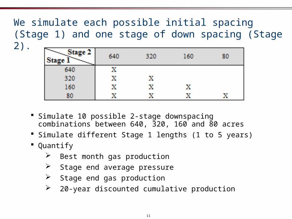
We simulate each possible initial spacing (Stage 1) and one stage of down spacing (Stage 2).

Simulate 10 possible 2-stage downspacing combinations between 640, 320, 160 and 80 acres

Simulate different Stage 1 lengths (1 to 5 years) Quantify

Best month gas production Stage end average pressure Stage end gas production 20-year discounted cumulative production

12

UGR provided a geostatistical study completed by Schlumberger.

A variogram analysis was performed to generate possible representations

of porosity, permeability and net pay at interwell locations and determine the

correlation coefficients between wells separated by specific distances.

13

Agenda


Reservoir Model

Decline Curve Model

Decision Model

14

To facilitate the integration of the reservoir and decision models, simulated production was fit with decline curves.

Modeled with hyperbolic decline with switch to exponential decline to account for long transient decline period in unconventional reservoirs.

Wrote VBA code coupled to the Solver add-in of Excel to perform the decline curve regression.

Integrated with the reservoir modeling software.

Determined decline parameters and the associated distribution functions for input to the decision model.

1000 Res. Sims.

Stages 1&2

Fit Decline Curves

Means

Std Devs

Correlation

Decision Model

Optimal Stage 1 Spacing

Optimal Stage 2 Spacing for every possible Stage 1 scenario

15

The decline curve model begins with hyperbolic and transitions to exponential.

Decline curve analysisperformed on simulated20-year production data

Decline curve analysisperformed on simulatedStage 1 production data

11 /( ) ( ) bi iq t q bDt

1 00

0

11

/ ( )( ) ( ) b i

i ii

D t tq t q bDt Exp

bDt

If

Else

0t t

16

Let’s look at example simulation results for a Stage 1 spacing of 160 acres and the downspacing to 80 acres.

Run # Qi Di b Qi Di b to Qi Di b to(MMscf/year) (1/year) (MMscf/year) (1/year) (year) (MMscf/year) (1/year) (year)

1 579.2874521 19.51090217 2.690628236 308.5480717 4.121016699 1.301250553 4.751228104 346.0439358 6.843065318 1.564714931 4.5350136512 542.6534094 33.88089553 2.422389906 188.988 3.781807468 1.058241967 4.890533543 246.732 3.458845905 0.896507401 5.402045533 871.8456112 31.21065924 2.059631195 245.82 3.453541961 0.971992644 4.801504711 130.7723691 5.224703792 1.348292046 4.5003537694 420.2300392 22.44841094 2.300467581 188.592 3.813929073 1.124899592 4.666791726 173.7034827 14.51516452 1.797626996 4.7367308695 2535.906503 17.39852897 2.294272579 870.768 2.717331129 0.664045369 5.425216524 679.776 2.945139966 0.753600142 5.2573731056 846.1461387 44.1652131 2.164888656 188.544 3.024928536 0.871280503 4.783820909 135.708 2.575778766 0.868591536 19.77728547 1588.075917 12.95321774 2.375993987 687.84 2.767017883 0.656140806 5.399116632 482.4354848 7.243769523 1.533511175 4.4556962698 576.3827579 24.15399374 2.421788008 216.432 3.281707069 0.917471412 5.109017075 340.764 3.40667185 0.889870016 5.4151051119 7586.392338 4788.801582 2.178530837 296.2191602 6.624513622 1.735553512 4.639650336 639.624 2.805006821 1.002975821 5.30083840210 907.1772116 28.53938468 2.636087741 394.0256512 4.246629735 1.402267432 4.757356074 542.6397941 4.06565545 1.383995579 4.733229303995 593.3805656 31.03630572 2.36376357 197.928 3.429690381 0.881695517 5.168412374 228.5401758 3.817650616 0.970830127 4.88368138996 927.9372273 20.79262045 2.452740163 388.5374808 3.54174877 0.937860863 4.831228351 214.104 4.270236876 1.202564543 4.670732554997 155.591259 24.49342232 3.362167267 122.878687 6.979508762 1.782815513 4.741082858 63.45625549 13.02056896 1.93040798 5.280391008998 363.1041289 15.02056635 3.090313614 263.8653135 4.313030498 1.467712222 4.801183333 206.680888 14.42168511 1.919068768 5.255246019999 291.6031431 26.38794043 2.862811213 148.3424682 4.301344216 1.51852206 4.851416881 197.3225363 7.421355324 1.741289624 4.6789230631000 1700.563667 74.8742782 2.26251908 431.8316211 4.320019231 1.438282928 4.692377946 540.1500354 5.889229449 1.629779861 4.56326565

Qi Di b Qi Di b to Qi Di b to(MMscf/year) (1/year) (MMscf/year) (1/year) (year) (MMscf/year) (1/year) (year)

mean 931.637011 467.9336135 2.550808628 298.5873497 4.562552452 1.269784744 4.85691977 339.2811346 5.138004238 1.241648883 5.038260373std dev 795.7231893 1997.154323 0.317095099 170.0123266 1.444083866 0.388458269 0.320296975 210.9332526 3.35466005 0.401489359 1.041973664

corr 0.446396055 0.428142198 0.684158879 0.426645293 -0.08335355 0.685885313

20 Year Decline Parameters20 Year Decline ParametersStage 2, Package 1 (80 acres) Stage 2, Package 2 (80 acres)Stage 1, Package 1 (160 acres)

20 Year Decline Parameters1st Year Decline Parameters 20 Year Decline Parameters

Stage 1, Well 3 (160 acres) Stage 2, Well 3 (80 acres) Stage 2, Well 4 (80 acres)

1st Year Decline Parameters

17

Stage 1 and 2 correlation results (1 Year and 3 Year Stage 1)…

Stage 1 Stage 2 ln(qi) ln(Di) b ln(qi) ln(Di) bSpacing Spacing

1 Year 640 640 0.23 0.43 0.82320 0.23 0.50 0.74 0.12 -0.08 0.17160 0.33 0.63 0.07 0.20 -0.06 -0.0380 0.36 0.67 0.03 0.24 0.12 -0.01

320 320 0.43 0.44 0.89160 0.45 0.58 0.46 0.41 -0.18 0.2280 0.57 0.73 0.30 0.56 -0.12 0.37

160 160 0.53 0.08 0.8180 0.66 0.63 0.68 0.64 -0.24 0.69

80 80 0.87 0.12 0.913 Year 640 640 0.62 0.51 0.95

320 0.61 0.46 0.90 0.30 -0.08 0.13160 0.60 0.60 0.11 0.42 -0.21 -0.0380 0.62 0.70 0.12 0.45 0.04 0.02

320 320 0.69 0.58 0.96160 0.69 0.39 0.46 0.42 -0.25 0.1180 0.67 0.67 0.26 0.57 -0.22 0.16

160 160 0.81 0.66 0.9380 0.80 0.66 0.73 0.61 -0.35 0.39

80 80 0.69 0.73 0.93

Correlation w/ Stage 1Stage 2: Package 1 Stage 2: Package 2

Correlation w/ Stage 1

18

This analysis provides several insights regarding learning.

Correlation in qi increases with:

Decreasing stage 1 spacing

Decreasing stage 2 spacing

Increasing stage 1 length

Our ability to learn about the initial decline rate for Package 2 is limited.

Our ability to learn about b is muted until we get down to about 160 ac for stage 1.

19

Agenda


Reservoir Model

Decline Curve Model

Decision Model

20

Our initial decision model allows for one stage of downspacing.

Key

Decision

Uncertainty

Calculation

Evocative

Value

Influence

Package 1(Stage 1)

Package 2(Stage 2)

qi (Pack 1)

D (Pack 1)

b (Pack 1)

qi (Pack 2)

b (Pack 2)

D (Pack 2)

NPV ($)

This is an “option” analysis. We make the Stage 2 decision after learning about Stage 1.

21

We make the following economic assumptions for illustrative purposes:

Gas Price $/MCF 5.50MC $/MCF 1.00FC MM $/yr/well 0.05Drilling Cost MM $/well 1.00Discout Rate 0.10

22

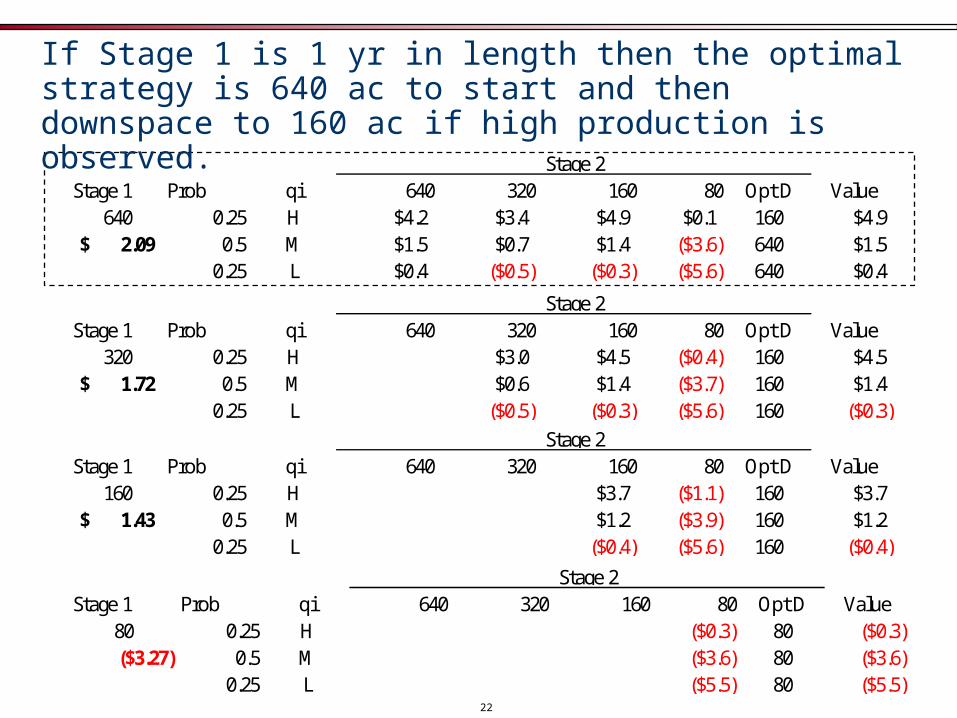
If Stage 1 is 1 yr in length then the optimal strategy is 640 ac to start and then downspace to 160 ac if high production is observed.

Stage 1 Prob qi 640 320 160 80 Opt D Value640 0.25 H $4.2 $3.4 $4.9 $0.1 160 $4.9

2.09$ 0.5 M $1.5 $0.7 $1.4 ($3.6) 640 $1.50.25 L $0.4 ($0.5) ($0.3) ($5.6) 640 $0.4

Stage 2

Stage 1 Prob qi 640 320 160 80 Opt D Value320 0.25 H $3.0 $4.5 ($0.4) 160 $4.5

1.72$ 0.5 M $0.6 $1.4 ($3.7) 160 $1.40.25 L ($0.5) ($0.3) ($5.6) 160 ($0.3)

Stage 2

Stage 1 Prob qi 640 320 160 80 Opt D Value160 0.25 H $3.7 ($1.1) 160 $3.7

1.43$ 0.5 M $1.2 ($3.9) 160 $1.20.25 L ($0.4) ($5.6) 160 ($0.4)

Stage 2

Stage 1 Prob qi 640 320 160 80 Opt D Value80 0.25 H ($0.3) 80 ($0.3)($3.27) 0.5 M ($3.6) 80 ($3.6)

0.25 L ($5.5) 80 ($5.5)

Stage 2

23

Notice that the dynamic strategy is about $660K better than a static 160 ac strategy.


2.09$ 0.5 M $1.5 $0.7 $1.4 ($3.6) 640 $1.50.25 L $0.4 ($0.5) ($0.3) ($5.6) 640 $0.4

Stage 2


1.43$ 0.5 M $1.2 ($3.9) 160 $1.20.25 L ($0.4) ($5.6) 160 ($0.4)

Stage 2

$2.09 MM - $1.43 MM = $0.66 MM

24

A three-year Stage 1 is worse than a 1-year Stage 1, but the dynamic strategy is still better.

Stage 1 Prob qi 640 320 160 80 Opt D Value640 0.25 H $1.4 $1.4 $3.4 ($1.0) 160 $3.4

$0.72 0.5 M $0.0 ($0.4) ($0.0) ($4.8) 640 $0.00.25 L ($0.6) ($1.4) ($2.1) ($7.2) 640 ($0.6)

Stage 2


$0.48 0.5 M ($0.4) ($0.0) ($4.8) 160 ($0.0)0.25 L ($1.4) ($2.1) ($7.2) 320 ($1.4)

Stage 2


$0.63 0.5 M $0.2 ($4.6) 160 $0.20.25 L ($2.0) ($7.0) 160 ($2.0)

Stage 2

Stage 1 Prob qi 640 320 160 80 Opt D Value80 0.25 H ($0.6) 80 ($0.6)($4.26) 0.5 M ($4.7) 80 ($4.7)

0.25 L ($7.1) 80 ($7.1)

Stage 2

25

Let’s look at a higher price environment.

Gas Price $/MCF 9.00MC $/MCF 1.00FC MM $/yr/well 0.05Drilling Cost MM $/well 2.00Discout Rate 0.10

26

With a 1-year stage 1, 640s are best to start and we downspace to 160s unless we see low production.


$4.14 0.5 M $2.8 $1.5 $3.2 ($5.2) 160 $3.20.25 L $0.8 ($0.6) $0.0 ($8.7) 640 $0.8

Stage 2

Stage 1 Prob qi 640 320 160 80 Opt D Value320 0.25 H $5.6 $8.6 $0.5 160 $8.6

$3.66 0.5 M $1.4 $3.0 ($5.4) 160 $3.00.25 L ($0.6) $0.0 ($8.7) 160 $0.0

Stage 2


$3.14 0.5 M $2.7 ($5.7) 160 $2.70.25 L ($0.1) ($8.7) 160 ($0.1)

Stage 2

Stage 1 Prob qi 640 320 160 80 Opt D Value80 0.25 H $0.6 80 $0.6($4.60) 0.5 M ($5.2) 80 ($5.2)

0.25 L ($8.6) 80 ($8.6)

Stage 2

27

However, under a 3-year Stage 1 we should start with 160s and not downspace.

Stage 1 Prob qi 640 320 160 80 Opt D Value640 0.25 H $2.6 $2.7 $6.6 ($0.5) 160 $6.6

$1.67 0.5 M $0.2 ($0.5) $0.5 ($7.4) 160 $0.50.25 L ($1.0) ($2.2) ($3.1) ($11.5) 640 ($1.0)

Stage 2


$1.38 0.5 M ($0.5) $0.5 ($7.4) 160 $0.50.25 L ($2.2) ($3.1) ($11.5) 320 ($2.2)

Stage 2

Stage 1 Prob qi 640 320 160 80 Opt D Value160 0.25 H $7.8 $0.7 160 $7.8

$1.72 0.5 M $1.0 ($6.9) 160 $1.00.25 L ($2.9) ($11.3) 160 ($2.9)

Stage 2

Stage 1 Prob qi 640 320 160 80 Opt D Value80 0.25 H $0.2 80 $0.2($6.35) 0.5 M ($7.1) 80 ($7.1)

0.25 L ($11.4) 80 ($11.4)

Stage 2

28

We are able to integrate the reservoir model and the decision model via the use of decline curves.

The reservoir / decline curve studies show that we are able to learn about reservoir parameters.

Initial spacing and stage lengths are substitutes to some degree.

We believe we can learn about each decline curve parameter, but learning about initial production rate appears strongest.

Optimal dynamic development strategies may be worth millions more than static strategies.

In conclusion…

29

Future Plans

Refine reservoir model.

Expand decision model to allow for learning about all decline curve parameters.

Incorporate completion efficiency into the reservoir/decision modelling.

Construct an areal, multi-well model of the same reservoir to better model heterogeneity and interference between wells.

Incorporate pilot down spacing into the reservoir/decision modeling to determine the optimum number and length of pilots.

30

07 April 2010

Denver, CO

OPTIMIZING DEVELOPMENT STRATEGIES TO INCREASE RESERVES IN

UNCONVENTIONAL GAS RESERVOIRS

Presented to:RPSEA

Unconventional Gas Program

Prepared by:Duane McVay, Gulcan Turkarslan, and Rubiel Ortiz, Texas A&M University

J. Eric Bickel and Luis Montiel, The University of Texas at Austin

31

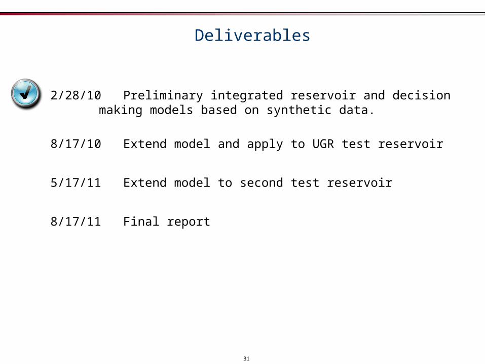
Deliverables

2/28/10 Preliminary integrated reservoir and decision making models based on synthetic data.

8/17/10 Extend model and apply to UGR test reservoir

5/17/11 Extend model to second test reservoir

8/17/11 Final report

32

Backup

33

Background

High risk associated with low-permeability gas sands Complex heterogeneities Variable reservoir properties Uncertain completion and stimulation efficiency

Sound development decisions needed Efficient completion practices Optimal well spacing

A trade-off between conserving capital and protecting the environment to avoid over drilling, but maximizing production by quickly achieving the optimum well spacing

34

Background

Determination of optimum development strategy in tight gas sands is technically challenging.

Large variability in rock quality

Wide range of depositional environments

Large number of wells

Limited reservoir information

Time & budget constraints

35

Background

Traditional methods for determining optimal well spacing

Statistical comparison of the performance of wells drilled at different spacings

Applicable only when sufficient production data from multiple infill programs are available

In emerging plays, historical infill programs are not available to evaluate optimal spacing with traditional methods.

36

Permeability Model

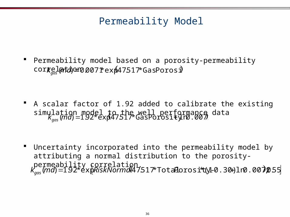
Permeability model based on a porosity-permeability correlation

A scalar factor of 1.92 added to calibrate the existing simulation model to the well performance data

Uncertainty incorporated into the permeability model by attributing a normal distribution to the porosity-permeability correlation.

55.0;0.0071ln 0.30)-(1*Porosity Total*517.47exp*92.1)( RiskNormalmdkgas

Porosity Gas*517.47exp*0071.0)( mdk gas

0.0071ln Porosity Gas*517.47exp*92.1)( mdk gas

38

Drainage Area Aspect Ratio (Y/X)

39

Reservoir Model Features

Distance between wells

The wells to be modeled were selected based upon the most prevalentseparation distance from well 1

40

Reservoir Model Features

Only one new well is modeled for each stage (i.e., 4 wells/section)

640 acres – Well 1



80 acres – Well 4

Each set of four wells are modelled individually but sampled from the same reservoir property distributions

Move to backup

41

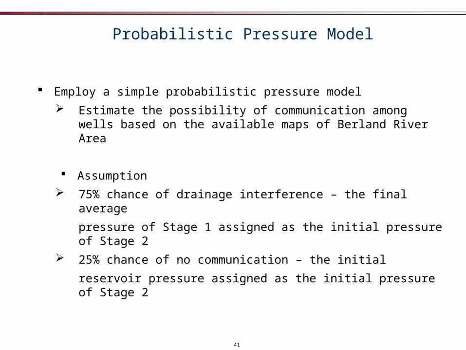
Probabilistic Pressure Model

Employ a simple probabilistic pressure model

Estimate the possibility of communication among wells based on the available maps of Berland River Area

Assumption

75% chance of drainage interference – the final average

pressure of Stage 1 assigned as the initial pressure of Stage 2

25% chance of no communication – the initial

reservoir pressure assigned as the initial pressure of Stage 2

07 April 2010 Denver, CO OPTIMIZING DEVELOPMENT STRATEGIES TO INCREASE RESERVES IN UNCONVENTIONAL GAS RESERVOIRS Presented to: RPSEA Unconventional Gas.

Documents

single phase reservoir

reservoir parameters

integrated reservoir

reservoir layers

single simulation model

client confidentialwe

decision tress

optimal development