05415666

8/4/2019 05415666

http://slidepdf.com/reader/full/05415666 1/10

1348 IEEE TRANSACTIONS ON BIOMEDICAL ENGINEERING, VOL. 57, NO. 6, JUNE 2010

Thyroid Segmentation and Volume Estimationin Ultrasound Images

Chuan-Yu Chang∗ , Senior Member, IEEE , Yue-Fong Lei, Chin-Hsiao Tseng, and Shyang-Rong Shih

Abstract—Physicians usually diagnose the pathology of the thy-roid gland by its volume. However, even if the thyroid glands arefound and the shapes are hand-marked from ultrasound (US) im-ages, most physicians still depend on computed tomography (CT)images, which are expensive to obtain, for precise measurementsof the volume of the thyroid gland. This approach relies heavilyon the experience of the physicians and is very time consuming.Patients are exposed to high radiation when obtaining CT images.In contrast, US imaging does not require ionizing radiation andis relatively inexpensive. US imaging is thus one of the most com-monly used auxiliary tools in clinical diagnosis. The present studyproposes a complete solution to estimate the volume of the thyroidgland directly from US images. The radial basis function neuralnetwork is used to classify blocks of the thyroid gland. The integralregion is acquired by applying a specific-region-growing methodto potential points of interest. The parameters for evaluating thethyroid volume are estimated using a particle swarm optimizationalgorithm. Experimental results of the thyroid region segmenta-tion and volume estimation in US images show that the proposedapproach is very promising.

Index Terms—Particle swarm optimization (PSO), radial ba-sis function (RBF) neural networks, region growing, thyroidsegmentation.

I. INTRODUCTION

THE THYROID gland is a butterfly shaped organ and is

composed of two cone-like lobes. Thyroid gland belongsto the endocrine system, and is located in the neck just in front

of the larynx. It controls the secretion of the thyroid hormone,

which regulates the temperature of the human body, and greatly

affects childhood intelligence, growth, and adult metabolism.

Too much or too little thyroid hormone (due to a thyroid that

is too large or two small, respectively) causes pathological

changes. Therefore, physicians often diagnose abnormal symp-

toms of the thyroid gland by its volume.

Ultrasound (US) imaging is currently the most popular di-

agnostic tool. It is inexpensive and easy to use; it can fol-

low anatomical deformations in real time during biopsy and

Manuscript received September 21, 2009; revised December 10, 2009;accepted January 4, 2010. Date of publication February 17, 2010; date of current version May 14, 2010. This work was supported by the NationalScience Council, Taiwan, under Grant NSC 96-2221-E-224-070 and by theNational Taiwan University Hospital, Yunlin Branch, under Grant NTUHYL96.YC-001. Asterisk indicates corresponding author .

∗C.-Y. Chang is with the Department of Computer Science and InformationEngineering, National Yunlin University of Science and Technology, Yunlin640, Taiwan (e-mail: [email protected]).

Y.-F. Lei is with Coretronic Corporation, Hsinchu 300, Taiwan.C.-H. Tseng and S.-R. Shih are with the Department of Internal Medicine,

National Taiwan University Hospital, Taipei, Taiwan (e-mail: [email protected]).

Color versions of one or more of the figures in this paper are available onlineat http://ieeexplore.ieee.org.

Digital Object Identifier 10.1109/TBME.2010.2041003

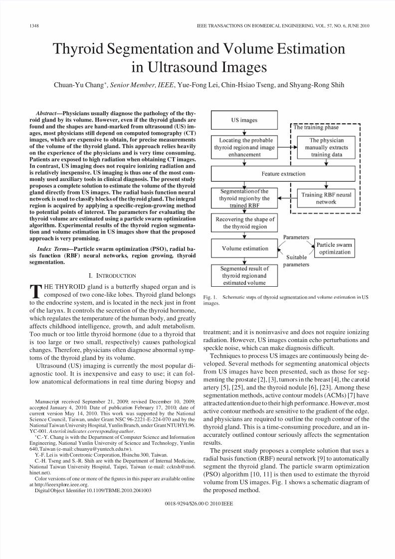
Fig. 1. Schematic steps of thyroid segmentation and volume estimation in USimages.

treatment; and it is noninvasive and does not require ionizing

radiation. However, US images contain echo perturbations and

speckle noise, which can make diagnosis difficult.

Techniques to process US images are continuously being de-

veloped. Several methods for segmenting anatomical objects

from US images have been presented, such as those for seg-

menting the prostate [2], [3], tumors in the breast [4], the carotid

artery [5], [25], and the thyroid nodule [6], [23]. Among these

segmentation methods, active contour models (ACMs) [7] have

attracted attention due to their high performance. However, most

active contour methods are sensitive to the gradient of the edge,

and physicians are required to outline the rough contour of the

thyroid gland. This is a time-consuming procedure, and an in-

accurately outlined contour seriously affects the segmentation

results.

The present study proposes a complete solution that uses a

radial basis function (RBF) neural network [9] to automatically

segment the thyroid gland. The particle swarm optimization

(PSO) algorithm [10, 11] is then used to estimate the thyroid

volume from US images. Fig. 1 shows a schematic diagram of

the proposed method.

0018-9294/$26.00 © 2010 IEEE

8/4/2019 05415666


CHANG et al.: THYROID SEGMENTATION AND VOLUME ESTIMATION IN ULTRASOUND IMAGES 1349

Fig. 2. Acquisition procedure. (a) Acquisition of longitudinal plane of

right thyroid lobe. (b) Acquisition of transversal plane of right thyroid lobe.(c) Segmented result in the right longitudinal plane by our proposed method.(d) Thickness and deepness axes in the right transverse plane.

In the training phase, the physicians must manually outline

the rectangular regions of interest (ROI) from the thyroid gland

and nonthyroid tissues. Six textural features extracted from the

ROIs are used to train the RBF neural network. The trained

RBF neural network can then automatically roughly classify the

thyroid regions from the US images. A specific-region-growing

method is then applied to retrieve the complete thyroid region.

Finally, based on the area of the segmented thyroid, the thick-

ness, and the depth of thyroid gland, the volume is estimated

using a PSO algorithm. Fig. 2 shows the acquisition procedure

and the two views of the thyroid gland of a patient. The US

probe is placed transversally and longitudinally to the left and

right thyroid lobe, respectively. Fig. 2(a) and (b) shows the ac-

quisition of longitudinal and transversal plane of right thyroid

lobe, respectively. Fig. 2(c) is the segmentation results in the

right longitudinal plane obtained using the proposed method,

and Fig. 2(d) shows the thickness and deepness axes in the right

transverse plane.

The rest of this paper is organized as follows. In Section II,

the details of the adaptive weighted median filter (AWMF) [13],

RBF neural network [9], reconstruction stages, and PSO algo-

rithm [10], [11] are described. Section III presents the experi-ment results. Conclusions are given in Section IV.

II. THYROID SEGMENTATION AND

VOLUME-ESTIMATION APPROACH

In order to directly estimate the thyroid volume from US im-

ages, thyroid segmentation must be accurate. Keramids et al.

extracted the local binary pattern (LBP) features from the ROI

of the thyroid and applied a k-nearest neighbor (k-NN) algo-

rithm to segment the thyroid gland. However, the segmented

thyroid glands are messy [23] and their method cannot extract

the complete thyroid gland. Therefore, in this paper, a com-

Fig. 3. (a) Original US image. (b) Horizontal projection of the US image.(c) Result of locating a probable thyroid region.

plete solution for segmenting thyroid glands is proposed. The

methods for thyroid segmentation and volume estimation are

presented in this section. There are five major steps, which are

as follows: 1) locating the probable thyroid region and image

enhancement; 2) feature extraction; 3) training RBF neural net-

works; 4) thyroid recovery; and 5) volume estimation. Detailsof these processes are described next.

A. Locating Probable Thyroid Region and Image Enhancement

In thyroid US images, low visual quality greatly affects the

segmentation and the volume estimation results. A preprocess-

ing step is thus required to enhance and locate the probable

thyroid region. The preprocessing steps are as follows: 1) locat-

ing the probable thyroid region; 2) applying an AWMF [13] to

reduce speckles; 3) applying two morphological operations [15]

to enhance the filtering result; and 4) compensating for different

US images according to the intensity template of the thyroid

region.1) Locating Probable Thyroid Region: In a thyroid US im-

age, the thyroid gland is always in the middle, below the bright

part and above the dark part of the image. Two reference values

(R1 and R2 ) are defined to locate the probable thyroid region.

R1 is the row index with the largest average intensity in the

horizontal projection of the US image. R2 is the first row index

with an average intensity of zero from the top to bottom in the

horizontal projection of the US image. The probable thyroid

region is located between the R1 th row and the R2 th row of the

US thyroid image. An example of locating a probable thyroid

region in an US thyroid image is shown in Fig. 3.

2) Adaptive Weighted Median Filter: Therole of preprocess-ing is to remove the speckle noise and to reduce the influence

of feature extraction. AWMF [13] is easy to use, has fewer free

parameters, and preserves small details better than other nonlin-

ear space-varying filters. Thus, an AWMF is applied to remove

inevitable speckle noise and to enhance the probable thyroid re-

gion in the US images. AWMF is conducted on a fixed moving

mask with the weights adjusted according to the local statistics.

For a mask with a size of M × M , the weight coefficient wi , j

at position (i, j) is given by

wi, j = w0

−gDσ 2

x, y

µx, y (1)

8/4/2019 05415666



where µx ,y and σ2x, y are the mean and variance of the M × M

window centered in the(x,y) pixel, respectively. w0 is the central

weight, g is a scale factor, [·] is round-to-nearest function, and

D is the Euclidean distance from the pixel point to the centre

of the mask. If the weights are negative, they are set to zero.

A 9 × 9 mask and parameters w0 = 10 and g = 0.25 are

used in this study [14]. The adaptive weighted median in anM × M region {I i ,j } is defined as the pure median of the

extended sequence formed by taking each term I i ,j , wi ,j times,

where {wi ,j } are the corresponding weight coefficients. For

example, if w1,1 = 2, w1,2 = 3, w2,1 = 3, and w2,2 = 1, the

weighted median of the mask {I 11 , I 12 , I 21 , I 22 } is given by

median {I 11 , I 11 , I 12 , I 12 , I 12 , I 21 , I 21 , I 21 , I 22 } = I 12 .

3) Morphological Operation: A set of 3 × 3 closing and

opening operators [15] were applied to remove the redundancy

enhanced by AWMF.

4) Gray-Level Compensation: The variation of the gray

level of the thyroid region in the US image greatly affects the

segmentation results [16]. A gray-level compensation technique

is thus applied to adjust the intensity of the probable thyroid re-gion. In thyroid US images, the intensities of skin/fat are larger

than those of other tissue. In general, the skin area occupied

20% of a thyroid US image. Hence, the normal-reference gray

level GLN is defined as the half gray level of an 8-bit image

(GLN = 128 in this study). The average value of the top 20%

pixels (in intensity) in the test image T (x,y) is regarded as the

test-reference gray level GLT . Accordingly, the intensity of the

test image is adjusted by the value between the normal-reference

gray level and the test-reference gray level using

T (x, y) =

255, if T (x, y)

−∆GL > 255

0, if T (x, y) − ∆GL < 0T (x, y) − ∆GL, otherwise

(2)

where ∆GL = GLN − GLT , x = 1, 2, . . . , H , and y = 1, 2,

. . . , W , where H and W denote the height and width of the

probable thyroid region, respectively.

B. Feature Extraction

Textural features contain important information that can be

used for the analysis andexplanationof US images. In this paper,

physicians manually extracted 2n ROIs with a size of M ×

M (n thyroid ROIs and n nonthyroid ROIs) from the probable

thyroid region. Various feature-extraction methods have been

implemented and analyzed. Six discriminative textural features

were then extracted from the selected ROIs: the Haar wavelet

[15], coefficient of local variation, histogram, block difference

of inverse probabilities (BDIPs) [17], and normalized multiscale

intensity difference (NMSID) [18]. These features are applied

to the RBF neural network to classify the thyroid region, as

described in Section II-C. These features are described in more

detail as follows.

1) Haar Wavelet Features: The Haar wavelet features are

significant features for segmentation in US images [19]. The

mean and the variance of the low-low-frequency subband (LL

band) were computed as follows [15] :

Mean of LL band : µx, y =1

M 2

(x, y )∈B

I (x, y) (3)

Variance of LL band : σ2x, y =

1

M 2

(x, y )∈B

(I (x, y)−

µx, y )2

(4)

where I (x, y) denotes the intensity of a pixel (x,y) in the ROI

block, which has passed through the Haar transformation, and

B denotes a block size of M × M .2) Coefficient of Local Variation Feature: The coefficient

of variation (CV) is a normalized measure of dispersion of a

probability distribution. Because the texture of thyroid glands

differs from those of other regions in the US image, CV is a

useful index to represent it. The coefficient of local variation of

a pixel located at (x, y) is defined as follows:

LCVx, y =σx, y

µx, y(5)

where µx ,y and σx, y are the local mean and standard deviation

of a pixel located at (x, y) with a block size of M × M ,respectively.

3) Histogram Feature: The histogram feature measures the

texture characteristics of an M × M block. Afterthe preprocess-

ing, the thyroid gland occupies most of the area in the probable

thyroid region. Thus, we extract the intensity of the largest area

and add a tolerance of ±

10. The value of the histogram feature

is defined as follows:

HF =

H + 10i= H −10 ,i= H

histo(i)

H = argi

max(histo(i)) (6)

where histo(i) is the value of the histogram for an intensity equal

to i of a block with a size of M × M . ±10 is a tolerance value

determined from experiments.

4) BDIP Feature: The BDIPs [17] uses local probabilities

in image blocks to measure local brightness variations of an

image. BDIP is defined as the difference between the number

of pixels in a block and the ratio of the sum of pixel intensities

in the block to the maximum in the block, i.e.,

BDIP =M 2 −(x, y )∈B I (x, y)

max(x, y )∈B I (x, y)(7)

where I (x, y) denotes the intensity of a pixel (x, y) and Bdenotes a block with a size of M × M .

5) NMSID Feature: NMSID [18] is defined as the differ-

ences between the pixel pairs with horizontal, vertical, diagonal,

8/4/2019 05415666



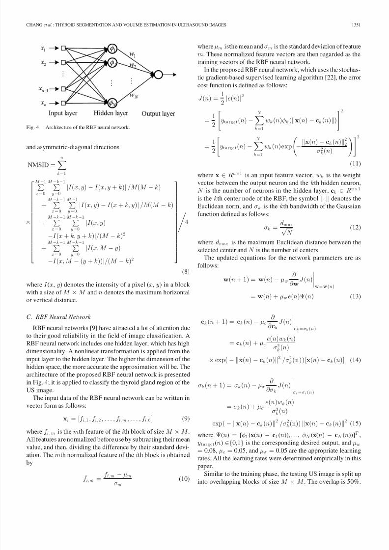
Fig. 4. Architecture of the RBF neural network.

and asymmetric-diagonal directions

NMSID =n

k =1

×

M −1

x= 0

M −k−1

y =0 |

I (x, y)

−I (x, y + k)

|/M (M

−k)

+M −k−1

x= 0

M −1y = 0

|I (x, y) − I (x + k, y)| /M (M − k)

+M −k−1

x= 0

M −k−1y =0

|I (x, y)

−I (x + k, y + k)|/(M − k)2

+M −k−1

x= 0

M −k−1y =0

|I (x, M − y)

−I (x, M − (y + k))|/(M − k)2

4

(8)

where I (x, y) denotes the intensity of a pixel (x, y) in a block

with a size of M × M and n denotes the maximum horizontal

or vertical distance.

C. RBF Neural Network

RBF neural networks [9] have attracted a lot of attention due

to their good reliability in the field of image classification. A

RBF neural network includes one hidden layer, which has high

dimensionality. A nonlinear transformation is applied from the

input layer to the hidden layer. The higher the dimension of the

hidden space, the more accurate the approximation will be. The

architecture of the proposed RBF neural network is presented

in Fig. 4; it is applied to classify the thyroid gland region of theUS image.

The input data of the RBF neural network can be written in

vector form as follows:

xi = [f i, 1 , f i, 2 , . . . , f i, m , . . . , f i, 6 ] (9)

where f i , m is the mth feature of the ith block of size M × M .All features are normalized before use by subtracting their mean

value, and then, dividing the difference by their standard devi-

ation. The mth normalized feature of the ith block is obtained

by

¯f i, m =

f i, m

−µm

σm (10)

where µm isthe mean and σm is the standard deviation of feature

m. These normalized feature vectors are then regarded as the

training vectors of the RBF neural network.

In the proposed RBF neural network, which uses the stochas-

tic gradient-based supervised learning algorithm [22], the error

cost function is defined as follows:

J (n) = 12

|e(n)|2

=1

2

ytarget(n) −

N k =1

wk (n)φk (x(n) − ck (n))

2

=1

2

ytarget(n) −

N k =1

wk (n)exp

−x(n) − ck (n)2

2

σ2k (n)

2

(11)

where x ∈ Rn×1 is an input feature vector, wk is the weight

vector between the output neuron and the kth hidden neuron,

N is the number of neurons in the hidden layer, ck ∈ Rn

×1

is the kth center node of the RBF, the symbol · denotes the

Euclidean norm, and σk is the kth bandwidth of the Gaussian

function defined as follows:

σk =dm ax√

N (12)

where dm ax is the maximum Euclidean distance between the

selected center and N is the number of centers.

The updated equations for the network parameters are as

follows:

w(n + 1) = w(n) − µw∂

∂ wJ (n)w=w(n)

= w(n) + µw e(n)Ψ(n) (13)

ck (n + 1) = ck (n) − µc∂

∂ ckJ (n)

ck =ck (n)

= ck (n) + µce(n)wk (n)

σ2k (n)

× exp( − x(n) − ck (n)2 /σ2k (n))[x(n) − ck (n)] (14)

σk (n + 1) = σk (n) − µσ

∂

∂σk J (n)

σ i =σ i (n)

= σk (n) + µσe(n)wk (n)

σ3k (n)

exp( − x(n) − ck (n)2 /σ2k (n)) x(n) − ck (n)2

(15)

where Ψ(n) = [φ1 (x(n) − c1 (n)),. . ., φN (x(n) − cN (n))]T ,

ytarget(n) ∈{0,1} is the corresponding desired output, and µw

= 0.08, µc = 0.05, and µσ = 0.05 are the appropriate learning

rates. All the learning rates were determined empirically in this

paper.

Similar to the training phase, the testing US image is split up

into overlapping blocks of size M × M . The overlap is 50%.

8/4/2019 05415666



Fig. 5. Structuring elements.

The normalized feature vectors of the overlapping block are

considered as input vectors in the trained RBF neural network.

The trained RBF neural network classifies the block into the

thyroid gland and the nonthyroid gland. For each thyroid block,

the number of thyroid blocks was calculated in its 8-nearest

neighbors. If the number is smaller than four, the block is re-

assigned to nonthyroid glands. Finally, the largest connected

component [20] is extracted from the classified US image. The

region of the largest connected component is considered as part

of the thyroid gland region.

D. Recovering Shape of Thyroid Region

Using the aforementioned procedures, a pure region of the

thyroid gland can be extracted (i.e., no pixels belong to the

nonthyroid gland region). However, the shape of the segmented

thyroid region is serrated, and thus, a refinement procedure is

required to recover the complete thyroid gland region. Con-

sequently, three specific reconstruction stages are applied to

recover the complete shape of the thyroid gland.

The first reconstruction stage is filtering out the blocking

shape of the segmented thyroid region. Let Bi , i = 1, 2, 3,

4 represent the four structuring elements, as shown in Fig. 5.

Entries marked by “×” indicate the “do not care” condition.The procedure consists of implementing the following

equation:

X i = (A ∗ Bi ) i = 1, 2, 3, 4 (16)

where A is the segmented thyroid region and ∗ denotes a match

operator [15]. The match operator is a morphological operator

designed to locate simple shapes within an image. A structuring

element is said to have found a match in the thyroid gland region

if the 3 × 3 region under the structuring element mask at that

location matches the pattern of the mask. For a particular mask,

a pattern match occurs when the center of the 3 × 3 region in the

thyroid gland region is 0, and the five pixels under the shadedmask elements are 1. The result of filtering out the blocking

shape of the segmented thyroid region A, denoted by S (A), is

thus

S (A) =

4∪

i= 1X i

∪ A. (17)

Fig. 6 shows the procedure given in (16) and (17). The origin

of each structuring element is at its center.

The second reconstruction stage is based on the convex-hull

concept [15]. Fig. 7 shows the four structuring elements of a

convex hull. The general convex-hull algorithm does not take

the local statistical information of the structuring element into

account; the algorithm was thus improved here to consider this

Fig. 6. (a) Set A. (b)–(e) Results with the structuring elements. (f) Final resultof filtering out the blocking shape of the segmented thyroid region showing thecontribution of each structuring element.

Fig. 7. Structuring elements of the convex hull.

information. If a pattern match occurs, the criterion of convex-

hull-based region growing is examined. The criterion is defined

as follows:

|m0 − m1 | < T (18)

where m0 denotes the mean gray-level value of 3 pixels under

the shaded mask elements, m1 denotes the mean gray level value

of 6 pixels under the bright mask elements, and T is a threshold.

T is set to four from trial and errors experiments. If a 3 × 3

mask centered on pixel (x, y) conforms to this criterion, then

pixel (x, y) is included in the thyroid gland region.

The thyroid gland usually contains cysts and blood vessels,

making messy holes in the obtained image. A region filling op-

eration and a 7 × 7 closing morphological operation are applied

to fill these holes [15]. Using the aforementioned processes, the

complete thyroid gland can be obtained, as shown in Fig. 2(c).The thickness axis of the segmented thyroid is acquired using

the longest horizontal axis of the segmented thyroid. Let DL and

DR denote the thickness axis of segmented thyroid glands in

the left and right longitudinal plans of US images, respectively.

E. Volume Estimation

Since computed tomography (CT) imaging is expensive and

involves hazardous radiation, US imaging is the most com-

monly used auxiliary tool currently utilized in clinical diagnosis.

Hence, this study proposes a complete solution to estimate the

volume of the thyroid gland directly from US images. PSO is a

population-based stochastic optimization technique developed

8/4/2019 05415666



by Eberhart and Kennedy [10], [11], inspired by the social be-

havior of bird flocking or fish schooling. The PSO algorithm is

usually used to obtain a set of potential solutions that evolves to

approach a convenient solution (or set of solutions) for a prob-

lem. The PSO algorithm has been reported to have strengths of

fast convergence and robust stability over other evolutionary op-

timization mechanisms, such as genetic algorithms or ant colonyalgorithms [26]. Therefore, the PSO algorithm is here applied to

estimate the parameters of the thyroid volume equation, which

is defined by

VolumeUS = a × (AreaL × DL + AreaR × DR ) + b (19)

where a and b are scale and bias parameters that are estimated

by the PSO algorithm, respectively. AreaL and AreaR represent

the areas of the left and the right lobes of segmented thyroid

regions in the left and right longitudinal planes of US images,

respectively. With this optimization scheme, the scale and bias

parameters for volume estimation canbe directly estimated from

the US images. The fitness function of the PSO algorithm is

defined by

Fitness = |[a × (AreaL × DL + AreaR × DR ) + b]

− VolumeCT | (20)

where VolumeCT denotes the volume calculated from the CT

image. To calculate the actual thyroid volume, the thyroid re-

gions were manually outlined and verified by two experienced

radiologists from the CT images. The areas of all slices and the

interslice distance were then integrated to calculate the actual

volume of thyroid gland.

The particle velocity and position can be mathematically

modeled according to the following equations:

V id = w × V id + c1 × rand() × ( pid − xid )

+ c2 × rand() × ( pg d − xid ) (21)

xid = xid + V id (22)

where V id denotes velocity of the dth dimension of the ith

particle, w denotes the inertia weight, c1 and c2 are learning

constants, rand(·) is a uniformly distributed random number

between 0 and 1, xid denotes the current position of the ith

particle, pid denotes the ith particle ( pid is used to keep track of

the particle coordinates in the problem space which are associ-

ated with the best solution (fitness) it has achieved so far), and

pg d denotes the best solution (fitness) of the entire population.Fig. 8 shows the flow chart of the general PSO algorithm. There

are five major steps. The particle positions and velocities are

randomly initialized. The fitness function for each particle is

calculated and the best solution for each particle is updated.

III. EXPERIMENTAL RESULTS

Four experiments were performed to show the capability of

the proposed method. The images used for the experiments were

taken from the Division of Endocrinology and Metabolism at

National Taiwan University Hospital, Yunlin Branch. All US

images were captured with a Toshiba Xario SSA-660A instru-

ment with the following parameters: thyroid echo = 4–6 cm,

Fig. 8. Flowchart describing the general PSO algorithm.

linear transducer = 5–7.5 cm. CT images were captured with

a General Electric LightSpeed-16 scanner with the following

parameters: 120 kVp and 248–396 mA.

Since CT imaging is expensive and involves hazardous radi-

ation, only five patients underwent both the US and CT inspec-

tions. Accordingly, the testing dataset contains a total of 20 US

images and five CT image series from five patients; each CT

series contained 80 slices. An additional 20 US images taken

of five patients were used to train the RBFNN for segmenting

thyroid regions from US images. In the 20 training US images, a

total of 60 training patterns, including 30 thyroid tissues and 30

nonthyroid tissues extracted by an experienced physician, were

used to train the RBF neural network. The size of the extracted

ROI blocks was 16 × 16.For the classification task, the RBF neural network was im-

plemented with one output node and 90 hidden neurons. Two

convergence conditions of the RBF neural network were defined

as: 1) the maximum iteration was set to 10000 and 2) the correc-

tion value of synaptic weights was less than 0.00001. When one

of the two conditions was satisfied, the training procedure was

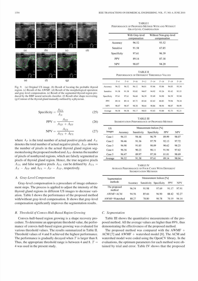
stopped. Fig. 9 shows the segmentation results obtained using

the proposed method. Fig. 9(a) shows the original US image,

which has serious speckle noise. The result of locating the prob-

able thyroid region is shown in Fig. 9(b). Fig. 9(c) and (d) shows

the results after image enhancement. Fig. 9(e) shows the clas-

sification result of the RBF neural network classifier. The seg-mented thyroid region after shape recovery is shown in Fig. 9(f).

Fig. 9(g) shows the contour of the thyroid gland outlined man-

ually by the physician. Fig. 9(g) and (f) are very similar.

In order to illustrate the segmentation performance of the pro-

posed method, five standardized measurements were adopted,

which are as follows: accuracy, sensitivity, specificity, positive

predictive value (PPV), and negative predictive value (NPV).

The five measurements are defined as follows:

Accuracy =ATP + ATN

AP + AN (23)

Sensitivity =

ATP

AP (24)

8/4/2019 05415666



Fig. 9. (a) Original US image. (b) Result of locating the probable thyroidregion. (c) Result of the AWMF. (d) Result of the morphological operationand gray-level compensation. (e) Result of the segmented thyroid region pro-duced by the RBF neural network classifier. (f) Result after shape recovering.

(g) Contour of the thyroid gland manually outlined by a physician.

Specificity =ATN

AN (25)

PPV =ATP

ATP + AFP(26)

NPV =ATN

ATN + AFN(27)

where AP is the total number of actual positive pixels and AN

denotes the total number of actual negative pixels. AT P denotes

the number of pixels in the actual thyroid gland region seg-mented using the proposed method and AFP denotes the number

of pixels of nonthyroid regions, which are falsely segmented as

pixels of thyroid gland region. Hence, the true negative pixels

ATN and false negative pixels AFN can be defined by AT N =AN − AFP and AFN = AP − ATP , respectively.

A. Gray-Level Compensation

Gray-level compensation is a procedure of image enhance-

ment steps. The process is applied to adjust the intensity of the

thyroid gland regions in different US images to decrease vari-

ation. Table I shows the performance of the proposed method

with/without gray-level compensation. It shows that gray-level

compensation significantly improves the segmentation results.

B. Threshold of Convex-Hull-Based Region Growing

Convex-hull-based region growing is a shape recovery pro-

cedure. To determine an appropriate threshold value, the perfor-

mance of convex-hull-based region growing was evaluated for

various threshold values. The results summarized in Table II.

Threshold values of 4 and 8 achieved the highest performance.

The performance is gradually decayed when T is larger than 8.

Thus, the appropriate threshold range is between 4 and 8. T =

4 was used in the present study.

TABLE IPERFORMANCE OF PROPOSED METHOD WITH AND WITHOUT

GRAY-LEVEL COMPENSATION

TABLE IIPERFORMANCE OF DIFFERENT THRESHOLD VALUES

TABLE IIISEGMENTATION PERFORMANCE OF PROPOSED METHOD

TABLE IVAVERAGE PERFORMANCE OF FOUR CASES WITH DIFFERENT

SEGMENTATION METHODS

C. Segmentation

Table III shows the quantitative measurements of the pro-

posed method. All the average values are higher than 89%, thus

demonstrating the effectiveness of the proposed method.

The proposed method was compared with the AWMF +ACM [7] and AWMF + watershed model [8]. The ACM and

watershed model were coded using the OpenCV library. In the

evaluations, the optimum parameters for each method were ob-

tained by trial and error. Table IV shows that the proposed

8/4/2019 05415666



Fig. 10. (a)–(c) Original US images. (d)–(f) Segmentation results of Fig. 11(a)–(c) using the proposed method shown with the overlapped contour,respectively. (g)–(i) Segmentation results using AWMF + ACM. (j)–(l) Seg-mentation results using AWMF + Watershed. (m)–(o) Contour of the thyroidgland manually outlined by a physician.

method outperforms the other segmentation methods. Because

of space limitations, only three of the 20 US image segmentation

results that were obtained are shown in Fig. 10. Fig. 10(a)–(c)

shows the original US images. The contours of the segmented

thyroid glands from the proposed method are superposed onto

the images in Fig. 10(d)–(f). Fig. 10(g)–(i) shows the segmenta-

tion results obtained using AWMF + ACM, while Fig. 10(j)–(l)

Fig. 11. Segmentation power of thyroid, where Az is equal to 0.891.

shows the segmented results obtained using AWMF + water-

shed. Finally, Fig. 10(m)–(o) shows the contours of the thyroid

glands manually outlined by a physician.The receiver–operating

characteristic (ROC) curves of thyroid segmentation are shown

in Fig. 11 [24]. Thevalue of true-positive fraction almost reaches

1 with a tiny loss of the false-positive fraction and the value of Az equals 0.891. The results show that the proposed method

correctly segments the thyroid gland region.

D. Volume Estimation

The detailed parameter settings for the PSO algorithm are

as follows: the maximum number of iterations was 200, the

population size was 12, the dimension of the search space was

set to 2, w = 1/(2×ln(2)), and c1 and c2 were both set to 0.5 +ln(2) [12]. To evaluate the accuracy of the estimated volume,

the difference ( Diff ) andthe MSE between the estimated volume

and the volume calculated from CT was applied. Diff and MSE

are defined as follows:

Diff =Gi − Gi

(28)

MSE =1

N

N i= 1

(Diff)2 (29)

where N is the case number, Gi is the volume estimation ob-

tainedusing theproposed method, and ˆ Gi is the volume obtained

from the CT images.

As mentionedearlier, only five CT seriesimages were taken of

five patients. To demonstrate the accuracy and efficiency of the

proposed volume estimation method, two cases were selected

randomly as training data and the others were used as testing

data. Theexperiment wasperformed ten times.The performance

of the proposed volume estimation method is shown in Table V.

The MSE values are below 0.9. In Table V, the training data are

in gray.

A low MSE indicates that the volume directly estimated from

US images is similar to that estimated from the CT images. The

proposed volume estimation method was compared with Brunn

et al.’s method [1], Wael et al.’s method [21], and standard

genetic algorithm [27], which are still used in clinical volume

estimation in most hospitals. Table VI shows the performance of

the volume estimation methods. The detailed parameter settings

for the genetic algorithm are summarized as follows: maximum

8/4/2019 05415666



TABLE VVOLUME ESTIMATION OF PROPOSED METHOD

TABLE VIPERFORMANCE WITH DIFFERENT VOLUME ESTIMATION METHODS

number of iterations: 500, population size: 200, crossover rate:

0.7, mutation rate: 0.0001, and two-point crossover: roulette

wheel selection. The fitness function was the same as that for

the PSO algorithm. The MSE value of the proposed method is

0.582, which indicates that it outperforms Brunn et al.’s, Waelet al.’s, and standard GA methods.

IV. CONCLUSION

US images are a widely used tool for clinical diagnosis, al-

though it is time consuming for physicians to manually segment

the thyroid gland region. The alternative to estimate the volume

of a thyroid gland using CT imaging is expensive and involves

hazardous radiation. Thus, a convenient system for thyroid seg-

mentation and volume estimation in US images is of interest.

The proposed method includes image enhancement processing

to remove speckle noise, which greatly affects the segmentation

results of the thyroid gland region obtained from US images.

The probable thyroid gland region is located in the US image,

and then, an RBF neural network is used to classify the re-

gion into thyroid and nonthyroid gland areas. Finally, a region

growing method is applied to recover an accurate shape of the

thyroid gland region. The experiment results show that the pro-

posed method can be used to segment the thyroid gland region

and to estimate thyroid volume directly from US images. Theproposed method offers two significant improvements: 1) it can

automatically segment the thyroid gland region from US images

and 2) it can accurately estimate the volume of the thyroid from

US images.

REFERENCES

[1] J. Brunn, U. Block, G. Ruf, I. Bos, W. P. Kunze, and P. C. Scriba, “Vol-umetric analysis of thyroid lobes by real-time ultrasound,” Dtsch Med

Wochenschr , vol. 106, pp. 1338–1340, Oct. 1981.[2] N. Hu, D. B. Downey, A. Fenster, and H. M. Ladak, “Prostate boundary

segmentation from3d ultrasound images,” Medical Physics, vol.30,no.7,pp. 1648–1659, Jul. 2003.

[3] B. Chiu, G. H. Freeman, M. M. A. Salama, and A. Fenster, “Prostate seg-mentationalgorithm using dyadic wavelet transform and discrete dynamiccontour,” Phys. Med. Biol., vol. 49, no. 21, pp. 4943–4960, Nov. 2004.

[4] D. R. Chen, R. F. Chang, W. J. Wu, W. K. Moon, and W. L. Wu, “3-Dbreast ultrasound segmentation using active contour model,” Ultrasound

Med. Biol., vol. 29, no. 7, pp. 1017–1026, Jul. 2003.[5] C. Baillard C. Barillot, P. Bouthemy, “Robust adaptive segmentation of

3d medical images with level sets,” Institut National de Recherche enInformatique et en Automatique (INRIA), Le Chesnay Cedex, France,Tech. Rep. 4071, Nov. 2000.

[6] D. E. Maroulis, M. A. Savelonas, D. K. Iakovidis, S. A. Karkanis,and N. Dimitropoulos, “Variable background active contour model forcomputer-aided delineation of nodules in thyroid ultrasound images,”

IEEE Trans. Inf. Technol. Biomed., vol. 11, no. 5, pp. 537–543, 2007.[7] M. Kass,A. Witkin, andD. Terzopoulos, “Snakes:Active contourmodels,”

Int. J. Comput. Vision, vol. 1, no. 4, pp. 321–331, 1987.[8] L. Vincent and P. Soille, “Watersheds in digital spaces: An efficient algo-

rithm based on immersion simulation,” IEEE Trans. Pattern Anal. Mach. Intell., vol. 13, no. 6, pp. 583–598, 1991.

[9] F. M. Ham and I. Kostanic, Principles of Neurocomputing for Science and Engineering. New York: McGraw-Hill, 2001.

[10] R. C. Eberhart and J. Kennedy, “A new optimizer using particle swarmtheory,”in Proc. 6thIEEE Int.Symp. Micro Mach. Human Science,pp.39–43, Oct. 1995.

[11] J. Kennedy and R. C. Eberhart, “Particle swarm optimization,” in Proc. IEEE Int. Conf. Neural Netw., vol. 4, pp. 1942–1948, 1995.

[12] M. Clerc, Standard PSO version 2006 . http://www.particleswarm.info/ Standard_PSO_2006.c, 2006.

[13] T. Loupas, W. N. McDicken, and P. L. Allan, “An adaptive weightedmedian filterfor speckle suppression in medical ultrasonic images,” IEEE Trans. Circuits Syst., vol. 36, pp. 129–135, Jan. 1989.

[14] Y. Chen,R. Yin,P.Flynn, andS. Broschat,“Aggressive regiongrowing forspeckle reduction in ultrasound images,” Pattern Recognit. Lett., vol. 24,pp. 677–691, Feb. 2003.

[15] R. C. Gonzalez and R. E. Woods, Digital Image Processing, 2nd ed.Englewood Cliffs, NJ: Prentice-Hall International Edition, 2002.

[16] R. L. Hsu, Mohamed Abdel-Mottaleb, and Anil K. Jain, “Face detectionin color image,” IEEE Trans. Pattern Anal. Mach. Intell., vol. 24, no. 5,May 2002.

[17] Y. D. Chum and S. Y. Seo, “Image retrieval using BDIP and BVLCmoments,” IEEE Trans. Circuits Syst. Video Technol, vol. 13, no. 9,pp. 951–957, Sep. 2003.

[18] E. L. Chen, P. C. Chung, C. L. Chen, H. M. Tsai, and C. I. Chang, “Anautomatic diagnostic system for CT liver image classification,” IEEE Trans. Biomed. Eng., vol. 45, no. 6, pp. 783–794, 1998.

[19] C. M. Wu, Y. C. Chen, andK. S. Hsieh, “Texturefeatures forclassificationof ultrasonic liver images,” IEEE Trans. Med. Imag., vol. 11, no. 2,pp. 141–152, Jun. 1992.

[20] L. D. Stefano andA. Bulgarelli, “A simpleand efficient connectedcompo-nents labeling algorithm,” in Proc. 10th Int. Conf. Image Anal., pp. 322–

327, 1999.

8/4/2019 05415666


05415666

Documents