Progress In Electromagnetics Research, PIER 42, 49–89, 2003 STABILITY OF CLASSICAL FINITE-DIFFERENCE TIME-DOMAIN (FDTD) FORMULATION WITH NONLINEAR ELEMENTS — A NEW PERSPECTIVE F. Kung and H. T. Chuah Faculty of Engineering Multimedia University Jalan Multimedia 63100 Cyberjaya, Selangor, Malaysia Abstract—In this paper new stability theorems for Yee’s Finite- Difference Time-Domain (FDTD) formulation are derived based on the energy method. A numerical energy expression is proposed. This numerical energy is dependent on the FDTD model’s E and H field components. It is shown that if the numerical energy is bounded, then all the field components will also be bounded as the simulation proceeds. The theorems in this paper are inspired by similar results in nonlinear dynamical system. The new theorems are used to prove the stability of a FDTD model containing non-homogeneous dielectrics, perfect electric conductor (PEC) boundary, nonlinear dielectric and also linear/nonlinear lumped elements. The theorems are intended to complement the well-known Courant-Friedrich-Lewy (CFL) Criterion. Finally it is shown how the theorems can be used as a test, to determine if the formulation of new lumped element in FDTD is proper or not. A proper formulation will preserve the dynamical stability of the FDTD model. The finding reported in this paper will have implications in the manner stability analysis of FDTD algorithm is carried out in the future. 1 Introduction 2 The New Stability Theorem 3 Application Example — Establishing the Stability of a Sourceless 3D Printed Circuit Board (PCB) Model 4 Extension of the Stability Theorem to 3D Model with Source

03.0301091.Kung
Dec 04, 2015
Stability of Classical Finite-Difference Time-Domain (FDTD) Formulation with Nonlinear Elements --- A New Perspective
Welcome message from author
This document is posted to help you gain knowledge. Please leave a comment to let me know what you think about it! Share it to your friends and learn new things together.
Transcript

Progress In Electromagnetics Research, PIER 42, 49–89, 2003
STABILITY OF CLASSICAL FINITE-DIFFERENCETIME-DOMAIN (FDTD) FORMULATION WITHNONLINEAR ELEMENTS — A NEW PERSPECTIVE
F. Kung and H. T. Chuah
Faculty of EngineeringMultimedia UniversityJalan Multimedia63100 Cyberjaya, Selangor, Malaysia
Abstract—In this paper new stability theorems for Yee’s Finite-Difference Time-Domain (FDTD) formulation are derived based onthe energy method. A numerical energy expression is proposed. Thisnumerical energy is dependent on the FDTD model’s E and H fieldcomponents. It is shown that if the numerical energy is bounded,then all the field components will also be bounded as the simulationproceeds. The theorems in this paper are inspired by similar results innonlinear dynamical system. The new theorems are used to prove thestability of a FDTD model containing non-homogeneous dielectrics,perfect electric conductor (PEC) boundary, nonlinear dielectric andalso linear/nonlinear lumped elements. The theorems are intended tocomplement the well-known Courant-Friedrich-Lewy (CFL) Criterion.Finally it is shown how the theorems can be used as a test, to determineif the formulation of new lumped element in FDTD is proper or not. Aproper formulation will preserve the dynamical stability of the FDTDmodel. The finding reported in this paper will have implications inthe manner stability analysis of FDTD algorithm is carried out in thefuture.
1 Introduction
2 The New Stability Theorem
3 Application Example — Establishing the Stability of aSourceless 3D Printed Circuit Board (PCB) Model
4 Extension of the Stability Theorem to 3D Model withSource

50 Kung and Chuah
5 Simulation Example
6 Conclusions
Appendix A. Finite-Difference Power Relation and V n
Appendix B. Stability for 3D FDTD Model
Appendix C. Negative Region for Resistive VoltageSource
References
1. INTRODUCTION
Classical Finite-Difference Time-Domain (FDTD) method using Yee’ssecond order formulation [1] has been successfully employed to modela wide range of microwave circuits and high-frequency printed circuitboard (PCB) assembly [2–5]. Traditionally to ensure numericalstability of the algorithm for a linear model, the Courant-Friedrich-Lewy (CFL) Criterion has to be fulfilled [3]. In an unstable algorithmthe computed E and H field components will increase without limitas the simulation progresses. The CFL Criterion has been derivedwith the assumption of homogeneous linear dielectric and unboundedmedium using Discrete Fourier Transform (DFT) (the Von Neumannapproach, [6, 9]). For a practical microwave circuit model the CFLCriterion serves as a rule-of-thumb at best. A few attempts recentlyextended the stability analysis to include linear dispersive media [6] andlinear lumped elements [7]. There is also an attempt to cast the FDTDmethod into iterative matrix equation [8]. The methods reportedstill rely on mathematical tools for linear systems (i.e., superpositionprinciple, DFT etc.) and will fail for nonlinear models. To-dateto the best of the authors’ knowledge, there is still no satisfactorytheory to explain the stability of FDTD formulation containing non-homogeneous dielectrics, boundary condition, nonlinear dielectric andalso linear and nonlinear lumped elements arranged in an arbitrarymanner. In this paper new stability theorems based on the energymethod are derived to address the issue. This work is inspiredby stability theory of dynamical systems [10], notably the SecondLiapunov Method [11–13]. Although not shown due to lack ofspace, the FDTD formulation is actually a discrete dynamical system.The proof of the theorems is shown in Appendix A and B andthe application is demonstrated in the main text. The theoremis used to prove what have been known throughout the years viasimulation, that the incorporation of certain lumped components such

Stability of classical FDTD formulation 51
as resistor, capacitor, diode and bipolar junction transistor in theFDTD framework is found to be stable. The theorems also show withease how a model containing non-homogeneous and nonlinear dielectricis stable. The theorems are intended to complement the CFL Criterionand the results of [6–8]. In Section 3 it is shown how the theoremsare used as a test, to determine whether the inclusion of new lumpedelement in FDTD is proper without performing lengthy simulation. Aproper formulation will preserve the stability of the FDTD model. Webegin by considering a 3D FDTD model for PCB or microwave circuitwithout any source (voltage or current source), with perfect electricconductor (PEC) as the model boundaries. The new theorems arestated and we proceed to prove the stability of the sourceless model.Then we extend the theorems to check the stability of a 3D FDTDmodel with voltage source. Finally a simple simulation example servesto substantiate the results.
Terminal
RF/MicrowaveConector
Casing,consistingof PEC
Spiralinductor
Active/Passivediscrete componentsand integrated circuits
Resonating
PCB
structures
Figure 1. A typical microwave circuit module.
2. THE NEW STABILITY THEOREM
Figure 1 shows a typical 3D FDTD model for microwave circuit PCBwithout any voltage or current source, with perfect electric conductor(PEC) as the model boundaries. Discretization and field componentsof each Yee’s Cell are shown in Figure 2. The model has nx, ny and nz

52 Kung and Chuah
Cube(nx,ny,1)
Cube(1,ny,n )
Cube(nx,1,1)
Cube(nx,1,n )
Cube(1,1,nz )
Cube(nx,1,1)
∆z
Cube(i,j,k)
Ez(i,j,k)
Ex(i,j,k)
Ey(i,j,k)
Hy(i,j,k)
Hz(i,j,k)
Hx(i,j,k
∆x
∆y
Ey(i,j,k+1)Ex(i,j,k+
Ez(i,j+1,k)
Ex(i,j+1,k)
Ey(i+1,j,k)
Ez(i+1,j,k)
1)
)
xy
z
z
z
Figure 2. Discretization of the 3D mode, and the standard Yee’s Cell(i, j, k) with associated field components.
cells along x, y and z axis respectively. Initially we assume the modelto be non-magnetic, i.e., µ = µo for all H fields. Also the cells are thesame in size. All the E and H field components within the model haveupdate equations given by the following form [3–5].
Hn+ 1
2
x(i,j,k) = Hn− 1
2
x(i,j,k) −∆tµ∇× Enx(i,j,k) (1a)
Hn+ 1
2
y(i,j,k) = Hn− 1
2
y(i,j,k) −∆tµ∇× Eny(i,j,k) (1b)
Hn+ 1
2
z(i,j,k) = Hn− 1
2
z(i,j,k) −∆tµ∇× Enz(i,j,k) (1c)
En+1x(i,j,k) = Enx(i,j,k) +
∆tεx(i,j,k)
[∇×Hn+ 1
2
x(i,j,k) − Jn+ 1
2
x(i,j,k)
](1d)
En+1y(i,j,k) = Eny(i,j,k) +
∆tεy(i,j,k)
[∇×Hn+ 1
2
y(i,j,k) − Jn+ 1
2
y(i,j,k)
](1e)
En+1z(i,j,k) = Enz(i,j,k) +
∆tεz(i,j,k)
[∇×Hn+ 1
2
z(i,j,k) − Jn+ 1
2
z(i,j,k)
](1f)
where in (1a)–(1f)
∇× Enx(i,j,k) =Enz(i,j+1,k) − Enz(i,j,k)
∆y−Eny(i,j,k+1) − Eny(i,j,k)
∆z(1g)
∇×Hn+ 12
x(i,j,k) =Hn+ 1
2
z(i,j,k) −Hn+ 1
2
z(i,j−1,k)
∆y−Hn+ 1
2
y(i,j,k) −Hn+ 1
2
y(i,j,k−1)
∆z(1h)

Stability of classical FDTD formulation 53
and so forth for y and z terms. Notice that the restriction for ε hasbeen removed, allowing it to vary according to location and orientation.Though not indicated, εr(i,j,k) (r = x, y, z) can also be functions of fieldcomponents at previous time-steps. Similarly the current density term
Jn+ 1
2
r(i,j,k) (r = x, y, z) also depends only on E and H field componentsat earlier time-steps.
Equations (1a)–(1f) will be known as the Canonical FDTD Formfor E andH field components. Update equations for many applicationscan usually be written in this form. Let us now introduce two newquantities, as defined by:
V n=∆V2
nz∑k=1
ny∑j=1
nx∑i=1
∑r=x,y,z
(εr(i,j,k)(E
nr(i,j,k))
2 + µo(Hn− 1
2
r(i,j,k))2
)
−Hn− 12
x(i,j,k)
[∆t∆y
(Enz(i,j+1,k) − Enz(i,j,k)
)
− ∆t∆z
(Eny(i,j,k+1) − Eny(i,j,k)
)]
−Hn− 12
y(i,j,k)
[∆t∆z
(Enx(i,j,k+1) − Enx(i,j,k)
)
− ∆t∆x
(Enz(i+1,j,k) − Enz(i,j,k)
)]
−Hn− 12
z(i,j,k)
[∆t∆x
(Eny(i+1,j,k) − Eny(i,j,k)
)
− ∆t∆y
(Enx(i,j+1,k) − Enx(i,j,k)
)]
(2a)
Pd=−∆Vnz∑k=1
ny∑j=1
nx∑i=1
{ ∑r=x,y,z
12
(En+1r(i,j,k) + Enr(i,j,k)
)Jn+ 1
2
r(i,j,k)
}(2b)
where ∆V = ∆x∆y∆z. In equation (2a), V n is known as the‘numerical energy’ of the 3D FDTD model at sequence n, it isanalogous to the stored electromagnetic energy in a physical system.It comprises all the E field components at time-step n and H fieldcomponents at time-step n− 1
2 . Similarly the numerical energy V n+1
comprises all E and H field components at time-step n+ 1 and n+ 12
respectively. In (2b) each term 12(En+1
r(i,j,k) + Enr(i,j,k))Jn+ 1
2
r(i,j,k) will beknown as ‘elemental dissipation’ since it is the approximate powerdensity dissipated by lumped element coinciding with Er(i,j,k) field.

54 Kung and Chuah
The negative sum of all elemental dissipation multiplied by ∆V is thetotal dissipation Pd of the model. Since all the boundaries are PEC, thenumerical energy within the model cannot escape from the boundary.The following theorems give the relationship between numerical energyand total dissipation, and the stability result.
Lemma 2.1 – Relationship between numerical energy and totaldissipation
Consider a 3D FDTD model with PEC boundaries of Figure 1.Given that all field update equations are of the form (1a)–(1f), withV n and Pd as defined in (2a) and (2b), then the following relation istrue:
V n+1 − V n = ∆t · Pd ✷ (3)
Lemma 2.2 – Positive definiteness of V n
Consider a 3D FDTD model with PEC boundaries of Figure 1.Given that all field update equations are of the form (1a)–(1f), thenV n is positive definite if and only if:
(a) εx(i,j,k) > 0, εy(i,j,k) > 0, εz(i,j,k) > 0 and µ = µo > 0. (4a)
(b) For ε = min{εx(i,j,k), εy(i,j,k), εz(i,j,k)} and cm = 1√µoε
, let:
∆t < min
1
cm√
2√
1∆y2
+ 1∆z2
,1
cm√
2√
1∆x2 + 1
∆z2
,1
cm√
2√
1∆x2 + 1
∆y2
(4b)
where i ∈ {1, 2, . . . , nx}, j ∈ {1, 2, . . . , ny}, k ∈ {1, 2, . . . , nz}. ✷
A function f(x) is positive definite when x = 0 implies f(x) > 0,and f(x) = 0 when x = 0 [13]. Note that x can be a vector or a scalar.The proofs for Lemma 2.1 and Lemma 2.2 are shown in Appendix A.In this context stability implies the FDTD algorithm for the 3D modelis both numerically and dynamically stable. This means that if wewere to reduce ∆t to zero or increase the time-step n to infinity, thesolution for E and H field components would always remain bounded.
Definition 2.1 – Stability of FDTD algorithm
Suppose we construct a vector Xn whose elements consist of all

Stability of classical FDTD formulation 55
E and H field components of the model:
Xn =
Enx(1,1,1)Enx(2,1,1)
...Enz(nx+1,ny+1,nz)
Hn− 1
2
x(1,1,1)
Hn− 1
2
x(2,1,1)...
Hn− 1
2
z(nx,ny ,nz+1)
(5a)
dimXn = M = 6nxnynz + 3(nxny + nxnz + nynz) + nx + ny + nz(5b)
Then the FDTD algorithm is stable when
∥∥Xn∥∥ ≤ C(T ) n = 1, 2, 3, . . . , N and N =T
∆t✷ (5c)
The symbol ‖x‖ means taking the ‘norm’ of a vector x [16],which is a measure of the ‘distance’ between x and the origin. C(T )is a positive real value which depends only on T , the maximumcomputation time. N = T/∆t is the maximum sequence. As∆t → 0, N will approach infinity. However (5c) dictates that C(T )must be finite as N approaches infinity as long as T is bounded.We allow C to be a function of T as certain solution of the FDTDcan increase with time. For instance when there is a source in themodel that increases with time, it is then reasonable to expect thefield components to gradually increase too. What (5c) means is thatthe solution remains bounded for finite time interval. If (5c) is notfulfilled as n increases, then the algorithm is not stable. Finally wedefine the stability theorem:
Theorem 2.3 – Stability theorem for 3D FDTD model
Consider a 3D FDTD model with PEC boundaries of Figure 1,if the model fulfills all the conditions in Lemma 2.2, then a sufficientcondition for it to be stable is Pd ≤ 0. ✷
The proof is given in Appendix B. The next section will shows howLemma 2.2 and Theorem 2.3 can be used to determine the stability ofa general 3D FDTD model for microwave circuits.

56 Kung and Chuah
3. APPLICATION EXAMPLE — ESTABLISHING THESTABILITY OF A SOURCELESS 3D PRINTED CIRCUITBOARD (PCB) MODEL
Assume a PCB model of Figure 1. The PCB model contains non-homogeneous dielectric, lumped resistors, lumped capacitors andnonlinear components such as PN junctions and bipolar junctiontransistors (BJTs). The FDTD update equations for E and H fieldsof all these elements can be found in [2–5]. Initially we will consider asourceless 3D FDTD model for reasons to be explained in Section 4.This means the model will not contain any source, such as the lumpedresistive voltage source [2]. We begin by computing the elemental
dissipation 12(En+1
r(i,j,k) +Enr(i,j,k))Jn+ 1
2
r(i,j,k) of each element, and show thatthis is always greater or equal to 0 under normal E and H fieldvalues. Furthermore we will also show that εr(i,j,k) is always positiveunder normal field values. Element meeting these two characteristicsis called proper. An elemental dissipation > 0 means that the elementis absorbing numerical energy from the model. When all the elementsare proper, the total dissipation Pd will be equal to 0 or negative,the condition of Theorem 2.3 will be fulfilled. We then limit thetime discretization ∆t as dictated by (4b) of Lemma 2.2. With thefinal condition met, Theorem 2.3 tells us that the model will bestable. For simplicity we assume the elements to be oriented in the+z direction. This can always be generalized to elements orientedalong other directions.
Lossless Linear Dielectric
For the Ez field of a lossless linear dielectric [3]:
En+1z(i,j,k) = Enz(i,j,k) +
∆tεrεo∇×Hn+ 1
2
z(i,j,k) (6a)
Comparing (6a) with the Canonical FDTD Form for Ez component:
Jn+ 1
2
z(i,j,k) = 0 and εz(i,j,k) = εrεo (6b)
Thus elemental dissipation 12(En+1
z(i,j,k) + Enz(i,j,k))Jn+ 1
2
z(i,j,k) = 0. Sinceεz(i,j,k) = εrεo > 0, the lossless linear dielectric formulation is proper.
Stability of classical FDTD formulation 57
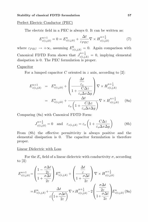
Perfect Electric Conductor (PEC)
The electric field in a PEC is always 0. It can be written as:
En+1z(i,j,k) = 0 = Enz(i,j,k) +
∆tεPEC
∇×Hn+ 12
z(i,j,k) (7)
where εPEC → +∞, assuming E0z(i,j,k) = 0. Again comparison with
Canonical FDTD Form shows that Jn+ 1
2
z(i,j,k) = 0, implying elementaldissipation is 0. The PEC formulation is proper.
Capacitor
For a lumped capacitor C oriented in z axis, according to [2]:
En+1z(i,j,k) = Enz(i,j,k) +
∆tεo
1 +C∆z
εo∆x∆y
∇×Hn+ 1
2
z(i,j,k)
= Enz(i,j,k) +∆t
εo
(1 +
C∆zεo∆x∆y
)∇×Hn+ 12
z(i,j,k) (8a)
Comparing (8a) with Canonical FDTD Form:
Jn+ 1
2
z(i,j,k) = 0 and εz(i,j,k) = εo
(1 +
C∆zεo∆x∆y
)(8b)
From (8b) the effective permittivity is always positive and theelemental dissipation is 0. The capacitor formulation is thereforeproper.
Linear Dielectric with Loss
For the Ez field of a linear dielectric with conductivity σ, accordingto [3]:
En+1z(i,j,k)=
1− σ∆t
2ε
1 +σ∆t2ε
Enz(i,j,k) +
∆tε
1 +σ∆t2ε
∇×Hn+ 1
2
z(i,j,k)
=Enz(i,j,k)+∆t
ε
(1+σ∆t2ε
)∇×Hn+ 12
z(i,j,k)−2
σ∆t2ε
1+σ∆t2ε
Enz(i,j,k) (9a)

58 Kung and Chuah
Comparing (9a) with Canonical FDTD Form:
εz(i,j,k) = ε
(1 +
σ∆t2ε
)(9b)
∆t
ε
(1 +
σ∆t2εo
)Jn+ 12
z(i,j,k) = 2
σ∆t2ε
1 +σ∆t2ε
⇒ J
n+ 12
z(i,j,k) = σEnz(i,j,k) (9c)
From (9b), εz(i,j,k) is always positive, but not the elemental dissipation.
Using x = Enz(i,j,k), d = σ∆t2ε and y = ∇ × Hn+ 1
2
z(i,j,k), the elementaldissipation is:
12
(En+1z(i,j,k) + Enz(i,j,k)
)Jn+ 1
2
z(i,j,k) =12
[1− d1 + d
x+∆t
ε(1 + d)y + x
](σx)
=σ
2(1 + d)
(2x+
∆tεy
)x (10)
This expression is not positive definite, certain combinations of xand y will cause it to become negative. To ensure that it is alwayspositive or 0, we need to introduce extra conditions. Requiring that
σ2(1+d)(2x+ ∆t
ε y)x ≥ 0:
For x ≥ 0 : y ≥ − 2ε∆tx⇒ ∇×Hn+ 1
2
z(i,j,k) ≥ −2ε
∆tEnz(i,j,k) (11a)
For x < 0 : y < − 2ε∆tx⇒ ∇×Hn+ 1
2
z(i,j,k) < −2ε
∆tEnz(i,j,k) (11b)
Most of the time the conditions of (11a) or (11b) are met,especially when σ is small (low loss at σ < 10). Extensive real-timeexaminations of elemental dissipation during FDTD simulation showthat the value is always positive for low to medium loss. We do nothave to explicitly impose conditions (11a) and (11b) during simulation.Equations (11a) and (11b) imply that current flowing through theelement is always limited. This is similar to an electrical circuit with afew paths having low resistance. Even though the low resistance pathcan support large current, the circuit configuration will tend to limitthe current through the paths, ensuring positive power dissipation.In the case of FDTD simulation, the system model will usually limitthe magnetic field components surrounding the electric field so thatpower dissipation is positive. However since finite-difference is only

Stability of classical FDTD formulation 59
an approximation to the actual Maxwell’s equations, it is expectedthat the elemental dissipation can become negative once in a while.Extensive simulations show that when σ is substantially greater than10, the elemental dissipation of (10) results in negative values once ina while. Most lossy dielectric material will have σ much smaller than1. When the elemental dissipation is negative, we could impose thefollowing equality (complying with (11a) and (11b)) to force it to 0:
∇×Hn+ 12
z(i,j,k) = −2ε
∆tEnz(i,j,k) (12a)
Applying (12a) to the update equation of (9a) would result in:
En+1z(i,j,k) = −Enz(i,j,k) (12b)
It is found that using (12b) for the case when elemental dissipation isnegative does not cause any noticeable change in the FDTD simulationresults. A typical flow of updating the E field for lossy dielectric withelemental dissipation checking and correction is shown in Figure 3.Therefore by modifying the update routine for linear dielectric withloss according to the flow of Figure 3, we could again conclude thatthe formulation is proper. A similar procedure can be used to showthat exponential time-stepping scheme [3] for high loss material is alsoproper, the details are omitted due to lack of space. Formulation such
as this where we limit ∇ × Hn+ 12
z(i,j,k) given Enz(i,j,k) will be known asconditionally proper.
Resistor
The update equation for a lumped resistive element of resistanceR is very similar to the form for linear dielectric with loss. We justreplace the term σ with ∆z
R∆x∆y [2].
En+1z(i,j,k) =
1− ∆t∆z2εoR∆x∆y
1+∆t∆z
2εoR∆x∆y
Enz(i,j,k)+
∆tεo
1+∆t∆z
2εoR∆x∆y
∇×Hn+ 1
2
z(i,j,k)
(13)
Using similar modified update routine as in Figure 3, the formulationfor resistor is also proper. Again simulation evidence shows that thisis not required most of the time, except for low resistance.

60 Kung and Chuah
Update Ez
21
22
2),,(1),,(1
11),,(
+
++
-+ ×∇
+
=
nkjiz
nkjiz
nkjiz HEE t
t
t
t
εσε
εσ
εσ
( ) ? 0),,(),,(1
),,(2≥++ n
kjizn
kjizn
kjiz EEEσ
End
Yes
Non
kjizn
kjiz EE ),,(1
),,( −=+
Elemental dissipation:
∆ ∆
∆∆
Start
Figure 3. Modified update routine for linear dielectric with nonzeroconductivity.
Diode or PN Junction
Consider a PN junction in parallel to the z-axis, with the updateequation for the corresponding electric field given by (using the firstorder approximation) [4]:
En+1z(i,j,k) = Enz(i,j,k) −
C1
B1(14)
C1 =N∆tε∆x∆y
InD −∆tεo∇×Hn+ 1
2
z(i,j,k),
B1 =∆t∆zε∆x∆y
(12dIDdV
(V n) +1
∆tCn
)+ 1
InD = Is
(exp
(V n
ηVT
)− 1
), V n = NEnz(i,j,k)∆z, VT =
kT
q
N is the orientation constant, it is +1 if the element is oriented in+z direction (i.e., positive current flows in +z direction) [4]. LetC2 = N∆t
εo∆x∆yInD, we could write (14) as:
En+1z(i,j,k) = Enz(i,j,k) +
∆tεoB1
∇×Hn+ 12
z(i,j,k) −C2
B1

Stability of classical FDTD formulation 61
Comparing this with the Canonical FDTD Form:
εz(i,j,k) = εoB1 =∆t∆z∆x∆y
(12dInDdV
+1
∆tCn
)+ εo
⇒ εz(i,j,k)
(Enz(i,j,k)
)
=∆t∆z∆x∆y
(Is
2ηVTexp
(NEnz(i,j,k)∆z
ηVT
)+
1∆tCn
)+εo (15a)
∆tεoB1
Jn+ 1
2
z(i,j,k) =C2
B1⇒ J
n+ 12
z(i,j,k) =εo∆tC2 (15b)
From (15a) the effective permittivity εz(i,j,k) is a function of Enz(i,j,k)and it is always positive, since Cn (the junction capacitance) and theexponential term always gives positive values. Let us form the followingproduct to examine the sign of elemental dissipation:
D =12
(En+1z(i,j,k) + Enz(i,j,k)
)Jn+ 1
2
z(i,j,k) =εo
2∆t
(2Enz(i,j,k) −
C1
B1
)C2 (16)
D is a function of Enz(i,j,k) and ∇ × Hn+ 12
z(i,j,k). Using x = Enz(i,j,k) and
y = ∇×Hn+ 12
z(i,j,k), a plot of D(x, y) versus x and y for a typical surface-mount Schottky diode HSMS-2820 [15] is shown in Figure 4. The diodeis oriented in −z direction (N = −1) and the range of x and y are:
x ∈ [−1000, 7500], y ∈ [−5000, 5000]
Using V = NEnz(i,j,k)∆z, the range for x corresponds to 0.55 to−4.125 Volts, from hard forward biased to hard reverse biased. Thisrange of x and y is typically encountered in simulation for low voltageRF circuits. We could enlarge the coverage if we wish, with similarresult obtained. It is seen from Figure 4 that D is weakly influenced byy. Figure 4 confirms that the elemental dissipation is always positiveor 0 for normal values of E field. In general it can be shown thatthis is also true for all practical diode models. Thus from the abovearguments, the diode or PN junction formulation is also proper.
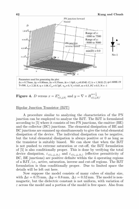
62 Kung and Chuah
x
y
D
Range of x:-1000 to 7500Range of y:-5000 to 5000
min(D) = 0.0
+z
Parameters used for generating the plot:x = 0.75mm, y = 0.80mm, z = 0.55mm, t = 1.0pS, εo=8.854E-12, k = 1.381E-23,
T=300, I = 2.2E-8, η = 1.08, C = 0.7pF, τ = 0, V = 0.65, m = 0.5, FC = 0.5, N = -1
0
5000
-50000
-1000
7500
N=-1
∆ ∆ ∆ ∆
s jo
q=1.608E-19
D j
PN junction forwardbiased
PN junction reverse biased
Figure 4. D versus x = Enz(i,j,k) and y = ∇×Hn+ 12
z(i,j,k).
Bipolar Junction Transistor (BJT)
A procedure similar to analyzing the characteristics of the PNjunction can be employed to analyze the BJT. The BJT is formulatedaccording to [5] where it consists of two PN junctions, the emitter (BE)and the collector (BC) junctions. The elemental dissipation of BE andBC junctions are summed up simultaneously to give the total elementaldissipation of the device. The individual dissipation can be negative,but the total elemental dissipation is always positive or 0 as long asthe transistor is suitably biased. We can show that when the BJTis not pushed to extreme saturation or cut-off, the BJT formulationof [5] is also conditionally proper. This is done by verifying the totaldevice dissipation, εz(ic,jc,kc) and εz(ie,je,ke) (effective permittivity ofBC, BE junctions) are positive definite within the 4 operating regionsof a BJT, i.e., active, saturation, inverse and cut-off regions. The BJTformulation is thus conditionally proper. Due to limited space thedetails will be left out here.
Now suppose the model consists of many cubes of similar size,with ∆x = 0.75 mm, ∆y = 0.8 mm, ∆z = 0.52 mm. The model is non-magnetic, but the dielectric constant is not uniform, with variation ofε across the model and a portion of the model is free space. Also from

Stability of classical FDTD formulation 63
(6b), (8b), (9b) and (15a), the effective permittivity εr(i,j,k) is alwaysgreater than εo. From this information, we conclude that the smallestpermittivity equals to εo as any dielectric which is not air will have εrgreater than unity. Using condition (4b) of Lemma 2.2:
cm =1√µoεo
∼= 1√(4π × 10−7)(8.854× 10⁻¹²)
∼= 2.99796× 10⁸
∆t < min
(cm√
2√
1∆y2
+1
∆z2
)−1
= 1.02835× 10⁻¹²,
(cm√
2√
1∆x2
+1
∆z2
)−1
= 1.0079× 10⁻¹²,
(cm√
2√
1∆x2
+1
∆y2
)−1
= 1.2905× 10⁻¹²
⇒ ∆t < 1.0079× 10⁻¹²
Compare this with CFL Criteria:
∆t <1
cm
√1
∆x2+
1∆y2
+1
∆z2
= 1.2573× 10⁻¹²
The new stability criterion has an increase in restriction by 19.84%.Finally we conclude that if all elements used have update equations ofthe above and ∆t < 1.0079× 10⁻¹², then according to Lemma 2.2 andTheorem 2.3, the model of Figure 1 will be stable. This means that ifthe initial E and H field components at time-step n = 0 is not 0, allfield components will remain bounded as we advance the time-step n.
Notice that throughout this section we only require the effectivepermittivity εr(i,j,k) of each E field component be positive. Thus thepermittivity can change with location, be a nonlinear function of fieldcomponents and yet the sourceless 3D model is still stable. So themethod proposed here could also be used to prove the stability ofmodel with non-homogeneous dielectric and nonlinear dielectric. Inthe next section, the case when there is a resistive voltage source inthe model will be considered.

64 Kung and Chuah
4. EXTENSION OF THE STABILITY THEOREM TO 3DMODEL WITH SOURCE
Suppose in addition to the elements mentioned in Section 3, the 3Dmodel of Figure 1 also contains a lumped resistive voltage source, withupdate equation for Ez field given by [2]:
En+1z(i,j,k) =
(1−Dz
1 +Dz
)Enz(i,j,k) +
∆tε(1 +Dz)
∇×Hn+ 12
z(i,j,k)
−[
2Dz
(1 +Dz)∆z
]V
(n+
12
)(17)
Where Dz = ∆t∆z2Rsε∆x∆y
, V (n+ 12) is the independent voltage source as
a function of time-step n and Rs being the source resistance. V (n+ 12)
can represent a constant d.c. source, a pulse, sinusoidal function andso forth. Converting (17) into the Canonical FDTD Form, we observethat the equivalent current density is:
Jn+ 1
2
z(i,j,k) =∆z
Rs∆x∆y
(Enz(i,j,k) +
V (n)∆z
)(18)
By introducing x = Enz(i,j,k), y = ∇ × Hn+ 12
z(i,j,k) and v = V (n+ 12)
∆z , theelemental dissipation can be written as:
Dn+ 12 (x, y, v) =
12
(En+1z(i,j,k) + Enz(i,j,k)
)Jn+ 1
2
z(i,j,k)
=∆z
2Rs∆x∆y· 11 +Dz
[2x+
∆tεy
]x
− ∆z2Rs∆x∆y
· 11 +Dz
[2Dzv −
∆tεy − 2(1−Dz)x
]v
(19)
Again this equation is indefinite, Dn+ 12 can be positive or negative.
When source element such as (17) is present, Pd can become positiveand from Lemma 2.1 the numerical energy V n of the model can increasewith time-step. Assuming v is a constant positive value (we canconsider it to be a d.c. voltage source), a plot of the region A in the x-yplane where elemental dissipation Dn+ 1
2 becomes negative is shown inFigure 5. A similar but inverted region can be easily plotted when vis a constant negative value.
A pertinent question is whether there is any further constraintapart from region A? In fact there is. The first constraint is the

Stability of classical FDTD formulation 65
x
y
0
A ( )xvDy zt−= ε2
vx −=
D less than 0 inthis region
A
Vs
+zRs
Is
∆
Figure 5. Negative region A of the resistive voltage source when v > 0and is constant.
current Is (see Figure 5) must not be more that Vs/Rs, which representsthe source current when the terminals are shorted. There are caseswhen source current can exceed this limit but for a properly designedcircuit Vs/Rs is usually the threshold. The second constraint is for thesource of (17) to continuously supply power to the model, elementaldissipation must always be negative or 0 at all sequence n. This meansif the (x, y) of sequence n result in Dn+ 1
2 ≤ 0, then (x, y) of sequencen + 1 must also result in Dn+ 3
2 ≤ 0. From Appendix C, we can showthat these requirements can be expressed mathematically as:
y <2ε∆t
(Dzv − x) (20a)
Dn+ 12 (x, y, v) ≤ 0 (20b)
xn+1 =(
1−Dz
1 +Dz
)xn +
∆tε(1 +Dz)
yn+ 12 − 2Dz
1 +Dzv ≥ −v (20c)
Using the criteria of (20a)–(20c), and assuming V (n + 12) = 1, a
new negative region, called B is shown in Figure 6a for Dz < 1 andFigure 6b for Dz > 1. When (x, y) is outside the shaded region B, theresistive voltage source will bound to stop supplying numerical powerto the model in future sequence and the E and H field componentswill start to decrease.
The negative regions B identified in Figure 6a and Figure 6bare still quite conservative, nevertheless it is sufficient for our nextargument. In order to have Dn+ 1
2 ≤ 0 for all n, the actual region couldbe smaller than shown. For a resistive voltage source to continuouslysupply numerical energy to the model, its state (x, y) must always be

66 Kung and Chuah
Parameters:x = 0.75mmy = 0.80mmz = 0.55mmt = 1.0ps
εr = 4.2Rs = 50Dz = 0.2465V/ z = v = 1.818.18
0x
y
v−( )xvDy zt
−= ε2
P1
P2
P3( )( )vxDy zt++= − 1ε
Coordinate of markers:
( )( )ztv DvP +−= 12,1
ε
( )0,2 vP −=
( )( )ztv DvP −−= 1, 2
3ε
0 4000−2000−4000
5 104
−5 104
0
Region where (20a)to (20c) are fulfilledfor (x,y).
15 104
B
∆∆∆∆
∆
∆
∆∆
∆
×
×
×
2000
v
xyt
−= ε2∆
Figure 6a. Negative region for resistive voltage source fulfilling (20a)to (20c), Dz < 1. P1 to P3 are marker points.
Parameters:x = 0.75mmy = 0.80mmz = 0.55mmt = 1.0ps
εr = 1.0Rs = 50Dz = 1.0353V/ z = v =
0x
y
v−
( )xvDy zt−= ε2
P1
P3
P2
Coordinate of markers:
( )( )ztv Dv +− 12, ε
( )0,v−
0 2000 4000−2000−4000
5×10
−5×104
0
Region where(20a) to (20c) arefulfilled for (x,y).
B ∆
∆∆∆∆
1.1818.18
∆P =1
2P =
P =3 ( )0,v
v
∆
Figure 6b. Negative region for resistive voltage source fulfilling (20a)to (20c), Dz > 1.
Stability of classical FDTD formulation 67
confined to B. Furthermore if the source V (n+ 12) is not constant, then
we can construct the negative region based on the largest magnitudeof V (n + 1
2). Negative regions for resistive voltage source whenV (n+1
2) is negative can be constructed in a similar manner using (20a)–(20c). The importance of the negative regions can be summed up asfollows. Suppose an FDTD model as in Figure 1 contains all proper orconditionally proper formulations and a few resistive voltage sources.Then initially the numerical energy V n of the system will increase.Since in Appendix B we have proven that V n is radially unbounded toall field components, a diverging V n will entails at least one or moreE or H field components that are increasing. Due to the propagatingnature of Maxwell’s equations, a field component that is increasingwithout limit will subsequently cause the rest of the model’s E andH field components to increase too. The important feature of thenegative regions is that it is bounded as long as the source voltage Vsis bounded and Rs greater than 0. If the increment of V n is not limitedby other dissipative elements in the model, (x, y) will eventually crossthe boundary of the negative region. Then the elemental dissipationof the resistive voltage source will bound to become positive againand the increment of numerical energy halts. Thus there is a built-in mechanism (due to Rs) in the resistive voltage source formulationto prevent uncontrolled increment of the field components. Withthis we can conclude that the general FDTD model with resistivevoltage sources will be numerically stable if and only if the following 3conditions are met:
1. Theorem 2.3 is fulfilled.2. There is no other source except resistive voltage sources.3. FDTD formulations of other elements are proper or conditionally
proper.
5. SIMULATION EXAMPLE
A simulation is carried out to verify the concepts discussed. Herea short conducting trace energized by a resistive voltage source isconnected to a parallel RC load. The PEC boundary is used in thisexperiment. The schematic and the top view of the FDTD model isshown in Figure 7. The simulated voltage across the resistive voltagesource and the load is shown in Figure 8(A), while the numerical energyV n is shown in Figure 8(B). In this model the resistive voltage sourceis immersed in the dielectric and is z directed. Its voltage functionis a single pulse of amplitude 3.3 V, active during 0–2100 ps and thenset to 0 beyond 2100 ps. As seen in Figure 8(B) when the voltage
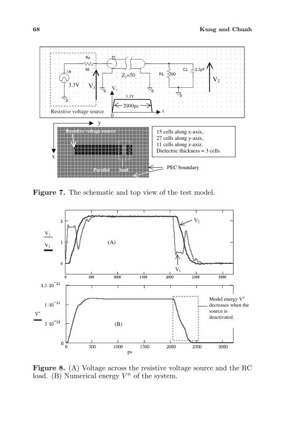
68 Kung and Chuah
Resistive voltage source
V1
V23.3V
15 cells along x-axis,27 cells along y-axis,11 cells along z-axiz.Dielectric thickness = 3 cells
Resistive voltage source
PEC boundary
x
y
Vs
t0
2000ps
3.3V
Zc=50
Parallel load
Figure 7. The schematic and top view of the test model.
V1
V2
Vn
ps
(A)
(B)
Model energy Vn
decreases when thesource isdeactivated.
V
V1
2
Figure 8. (A) Voltage across the resistive voltage source and the RCload. (B) Numerical energy V n of the system.

Stability of classical FDTD formulation 69
P1
P2
P3
n = 0
n = 2000
Negativeregion
x
y
Figure 9. Location of the state (x, y) for n = 0 to n = 2000 at aninterval of 10 time-steps.
source is active, V n increases rapidly and then saturates, as the ‘power’supplied by the source equals the ‘power’ dissipated by the resistors inthe model. During active stage the state (x, y) of the resistive voltagesource is determined from the correspondingE andH fields and plottedin the x-y plane of Figure 9. From the result we could clearly see thatthe coordinate never leaves the negative region. After the voltage Vsis deactivated, the resistive voltage source reverts to a normal resistormodel. We observe that the numerical energy V n of the model startsto decline, as now all the elements in the model are proper.
6. CONCLUSIONS
The theorems in Section 2 are useful. They overcome the limitationsof Von-Neumann approach, which result in the CFL Criterion. Firstand foremost, they can be used to determine and ensure the stability ofYee’s FDTD model for microwave circuit or high-speed PCB with thefollowing conditions: (a) Variable and nonlinear dielectric constant.(b) Containing linear and nonlinear lumped elements. (c) Includingthe effect of PEC boundary. In applying Theorem 2.3, the onlyrequirement for permittivity ε is that it must be positive for all E

70 Kung and Chuah
field components while the requirement for permeability µ is that itmust be equal to µo for all H field components.
Secondly, the conditions imposed on εr(i,j,k), Jn+ 1
2
z(i,j,k) and Pd inLemma 2.2 and Theorem 2.3 can be used as a test to check whetherthe FDTD formulation of a lumped element is proper. For a newlumped element, we can write its E field update equation in theCanonical FDTD Form, determine the equivalent current density and
compute its elemental dissipation 12(En+1
z(i,j,k) + Enz(i,j,k))Jn+ 1
2
z(i,j,k) againstall possible combinations of dependent field components as shown inSection 3. As long as the elemental dissipation is greater or equal to 0and εr(i,j,k) > 0, we know that the formulation is proper and will notcontribute to instability of the model.
The Von-Neumann and other linear approaches cannot be used toanalyze stability of the system under the above conditions of (a)–(c),and traditionally rule-of-thumbs are used to ensure that the FDTDmodel is stable. In addition, the approach presented here can also beextended to include:• Variable and nonlinear permeability.• Non-uniform cell size.• Dispersive elements and lumped inductors.• Absorbing boundary condition.
The first and second extension can be carried out by writingµ = µr(i,j,k) and reformulating the condition for V n to be positivedefinite. The third extension can be carried out by implement amonitoring algorithm much like Figure 3. The fourth extension canbe achieved by introducing a few layers of cells with conductivitybefore the PEC boundary. A better approach would be to introducemagnetic conductivity and magnetic current. Then formulate anabsorbing boundary condition (ABC) based on Perfectly MatchedLayer (PML) method [3]. Similar procedures as in the previous sectionscan be used to derive extended theorem incorporating magnetic loss
of 12
(Hn+ 1
2
r(i,j,k) +Hn− 1
2
r(i,j,k)
)Mnr(i,j,k), where Mn
r(i,j,k) is the corresponding
magnetic current density.The method does have some disadvantages. It will fail when there
is update equations for either E or H field that cannot be written inthe Canonical FDTD Form. Also the condition for ∆t is slightly morerigid than CFL Criterion. Finally the effect of absorbing boundarycondition based on mathematical formulation such as Mur’s ABC havenot been established. Efforts will be made to include this as well infuture research.
Stability of classical FDTD formulation 71
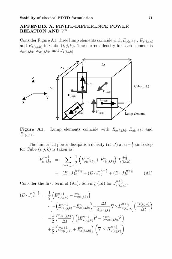
APPENDIX A. FINITE-DIFFERENCE POWERRELATION AND V N
Consider Figure A1, three lump elements coincide withEx(i,j,k), Ey(i,j,k)and Ez(i,j,k) in Cube (i, j, k). The current density for each element isJx(i,j,k), Jy(i,j,k), and Jz(i,j,k).
xy
z
Cube(i,j,k)
Lump element
Ez(i,j,k)
Ex(i,j,k)
Ey(i,j,k)
Hy(i,j,k)
Hz(i,j,k)
Hx(i,j,k)
xy
z
∆∆
∆
Figure A1. Lump elements coincide with Ex(i,j,k), Ey(i,j,k) andEz(i,j,k).
The numerical power dissipation density (E ·J) at n+ 12 time step
for Cube (i, j, k) is taken as:
Pn+ 1
2
(i,j,k) =∑
r=x,y,z
12
(En+1r(i,j,k) + Enr(i,j,k)
)Jn+ 1
2
r(i,j,k)
= (E · J)n+ 1
2x + (E · J)
n+ 12
y + (E · J)n+ 1
2z (A1)
Consider the first term of (A1). Solving (1d) for Jn+ 1
2
x(i,j,k):
(E · J)n+ 1
2x =
12
(En+1x(i,j,k) + Enx(i,j,k)
)·[−
(En+1x(i,j,k)−E
nx(i,j,k)
)+
∆tεx(i,j,k)
∇×Hn+ 12
x(i,j,k)
](εx(i,j,k)∆t
)
= −12
(εx(i,j,k)∆t
) ((En+1
x(i,j,k))2 − (Enx(i,j,k))
2)
+12
(En+1x(i,j,k) + Enx(i,j,k)
) (∇×Hn+ 1
2
x(i,j,k)
)

72 Kung and Chuah
Now let us introduce three new notations:(En · ∇ ×Hn+ 1
2
)(i,j,k)
=∑
r=x,y,z
Enr(i,j,k)∇×Hn+ 1
2
r(i,j,k) (A2)
(Hn+ 1
2 · ∇ × En)
(i,j,k)=
∑r=x,y,z
Hn+ 1
2
r(i,j,k)∇× Enr(i,j,k) (A3)
∇ ·(En+1 ×Hn+ 1
2
)(i,j,k)
= −(En+1 · ∇ ×Hn+ 1
2
)(i,j,k)
+(Hn+ 1
2 · ∇ × En+1)
(i,j,k)(A4)
In (A2)–(A4) the time-step is not critical, for instance we could replacen with n + 1 without affecting the validity. Using (A2) and summingup the x, y and z components, (A1) can be written in a more compactform:
−Pn+ 12
(i,j,k) =12
∑r=x,y,z
εr(i,j,k)
∆t
((En+1
r(i,j,k))2 − (Enr(i,j,k))
2)
−(En+1 · ∇ ×Hn+ 1
2
)(i,j,k)
−(En · ∇ ×Hn+ 1
2
)(i,j,k)
(A5)
Adding and subtracting (Hn+ 12 ·∇×En+1)(i,j,k) and (Hn+ 1
2 ·∇×En)(i,j,k)to the second and third terms on the right-hand side of (A5):(
En+1 · ∇ ×Hn+ 12
)(i,j,k)
=(Hn+ 1
2 · ∇ × En+1)
(i,j,k)
−∇ ·(En+1 ×Hn+ 1
2
)(i,j,k)
(A6a)(En · ∇ ×Hn+ 1
2
)(i,j,k)
=(Hn+ 1
2 · ∇ × En)
(i,j,k)
−∇ ·(En ×Hn+ 1
2
)(i,j,k)
(A6b)
Using (A3), (1a)–(1c), the first term on the right-hand side of (A6a),(A6b) can be expanded as:
(Hn+ 1
2 · ∇ × En+1)
(i,j,k)= −
∑r=x,y,z
µ
∆t
(−(H
n+ 12
r(i,j,k))2 + (H
n+ 12
r(i,j,k))2
)
+(Hn+ 1
2 · ∇ × En+1)
(i,j,k)(A7a)

Stability of classical FDTD formulation 73(Hn+ 1
2 · ∇ × En)
(i,j,k)= −
∑r=x,y,z
µ
∆t
((H
n+ 12
r(i,j,k))2 − (H
n− 12
r(i,j,k))2
)
−(Hn− 1
2 · ∇ × En)
(i,j,k)(A7b)
Finally substituting (A7a), (A7b), (A6a) and (A6b) into (A5), weobtain the desired expression for numerical power dissipation densityat Cube (i, j, k):
12∆t
[ ∑r=x,y,z
(εr(i,j,k)(E
n+1r(i,j,k))
2 + µ(Hn+ 1
2
r(i,j,k))2
)
− ∆t(Hn+ 1
2 · ∇ × En+1)
(i,j,k)
]
− 12∆t
[ ∑r=x,y,z
(εr(i,j,k)(E
nr(i,j,k))
2 + µ(Hn− 1
2
r(i,j,k))2
)
− ∆t(Hn− 1
2 · ∇ × En)
(i,j,k)
]
+12
{∇ ·
(En+1 ×Hn+ 1
2
)(i,j,k)
+∇ ·(En ×Hn+ 1
2
)(i,j,k)
}
= −Pn+ 12
(i,j,k) = −{ ∑r=x,y,z
12
(En+1z(i,j,k) + Enz(i,j,k)
)Jn+ 1
2
r(i,j,k)
}(A8)
Equation (A8) only applies to a single Yee’s cell at index (i, j, k).Now we determine the form for (A8) when sum up over all the cells.We could expand the expression in the third braces on the left-handside of (A8) using (A2)–(A4). For E and H field components at n andn+ 1
2 time steps:
∇ ·(En×Hn+ 1
2
)(i,j,k)
=∇·(En×Hn+ 1
2
)(i,j,k)x
+∇·(En×Hn+ 1
2
)(i,j,k)y
+∇ ·(En×Hn+ 1
2
)(i,j,k)z
=1
∆y
[Enx(i,j,k)H
n+ 12
z(i,j−1,k) − Enx(i,j+1,k)H
n+ 12
z(i,j,k)
]
+1
∆z
[Enx(i,j,k+1)H
n+ 12
y(i,j,k) − Enx(i,j,k)H
n+ 12
y(i,j,k−1)
]
+1
∆z
[Eny(i,j,k)H
n+ 12
x(i,j,k−1) − Eny(i,j,k+1)H
n+ 12
x(i,j,k)
]
74 Kung and Chuah
+1
∆x
[Eny(i+1,j,k)H
n+ 12
z(i,j,k) − Eny(i,j,k)H
n+ 12
z(i−1,j,k)
]
+1
∆x
[Enz(i,j,k)H
n+ 12
y(i−1,j,k) − Enz(i+1,j,k)H
n+ 12
y(i,j,k)
]
+1
∆y
[Enz(i,j+1,k)H
n+ 12
x(i,j,k) − Enz(i,j,k)H
n+ 12
x(i,j−1,k)
](A9)
The total sum ofnz∑k=1
ny∑j=1
nx∑i=1∇ · (En ×Hn+ 1
2 )(i,j,k) can be obtained by
considering the sum of each component. The details are not difficultbut very tedious; it will not be shown due to lack of space. For a 3Dmodel consisting of (nxnynz) cubes, it can be shown that:
nz∑k=1
ny∑j=1
nx∑i=1
∇ · (En ×Hn+ 12 )(i,j,k) =
1∆x
nz∑k=1
ny∑j=1
(Eny(nx+1,j,k)H
n+ 12
z(nx,j,k)− Eny(1,j,k)H
n+ 12
z(0,j,k)
− Enz(nx+1,j,k)Hn+ 1
2
y(nx,j,k)+ Enz(1,j,k)H
n+ 12
y(0,j,k)
)
+1
∆y
nz∑k=1
nx∑i=1
(Enz(i,ny+1,k)H
n+ 12
x(i,ny ,k)− Enz(i,1,k)H
n+ 12
x(i,0,k)
− Enx(i,ny+1,k)Hn+ 1
2
z(i,ny ,k)+ Enx(i,1,k)H
n+ 12
z(i,0,k)
)
+1
∆z
ny∑j=1
nx∑i=1
(Enx(i,j,nz+1)H
n+ 12
y(i,j,nz)− Enx(i,j,1)H
n+ 12
y(i,j,0)
− Eny(i,j,nz+1)Hn+ 1
2
x(i,j,nz)+ Eny(i,j,1)H
n+ 12
x(i,j,0)
)(A10)
Equation (A10) is also valid when En is replaced by En+1. Finally bysumming equation (A8) for all the cubes in a 3D model, we obtain thetotal numerical power relation:
12
nz∑k=1
ny∑j=1
nx∑i=1
[ ∑r=x,y,z
(εr(i,j,k)(E
n+1r(i,j,k))
2 + µ(Hn+ 1
2
r(i,j,k))2
)
− ∆t(Hn+ 1
2 · ∇ × En+1)
(i,j,k)
]

Stability of classical FDTD formulation 75
−12
nz∑k=1
ny∑j=1
nx∑i=1
[ ∑r=x,y,z
(εr(i,j,k)(E
nr(i,j,k))
2 + µ(Hn− 1
2
r(i,j,k))2
)
− ∆t(Hn− 1
2 · ∇ × En)
(i,j,k)
]
+∆t2
nz∑k=1
ny∑j=1
nx∑i=1
{∇ ·
(En+1×Hn+ 1
2
)(i,j,k)
+∇ ·(En×Hn+ 1
2
)(i,j,k)
}
= −∆tnz∑k=1
ny∑j=1
nx∑i=1
{ ∑r=x,y,z
12
(En+1r(i,j,k) + Enr(i,j,k)
)Jn+ 1
2
r(i,j,k)
}(A11)
It is understood that (A10) will be used to expand the thirdterm on the left-hand side of (A11). Equation (A11) is the finite-difference Poynting power relation for a 3D FDTD model with theupdate equations for E and H fields fulfilling the canonical form of(1a)–(1f). Both (A10) and (A11) are still formidable to apply. It willbe applied to a model with PEC boundary surfaces as shown in Figure1. All the following E field components on the boundaries will be zeroregardless of time-step n:
Enx(i,1,k), Enx(i,ny+1,k), E
nx(i,j,1), E
nx(i,j,nz+1) = 0
Eny(1,j,k), Eny(nx+1,j,k), E
ny(i,j,1), E
ny(i,j,nz+1) = 0
Enz(1,j,k), Enz(nx+1,j,k), E
nz(i,1,k), E
nz(i,ny+1,k) = 0
Substituting these components into (A10), we observe that:
nz∑k=1
ny∑j=1
nx∑i=1
{∇ ·
(En+1×Hn+ 1
2
)(i,j,k)
+∇ ·(En×Hn+ 1
2
)(i,j,k)
}= 0
(A12)
Thus putting (A12) into the numerical power relation (A11) yields:
12
nz∑k=1
ny∑j=1
nx∑i=1
[ ∑r=x,y,z
(εr(i,j,k)(E
n+1r(i,j,k))
2 + µ(Hn+ 1
2
r(i,j,k))2
)
− ∆t(Hn+ 1
2 · ∇ × En+1)
(i,j,k)
]
−12
nz∑k=1
ny∑j=1
nx∑i=1
[ ∑r=x,y,z
(εr(i,j,k)(E
nr(i,j,k))
2 + µ(Hn− 1
2
r(i,j,k))2
)

76 Kung and Chuah
− ∆t(Hn− 1
2 · ∇ × En)
(i,j,k)
]
= −∆tnz∑k=1
ny∑j=1
nx∑i=1
{ ∑r=x,y,z
12
(En+1r(i,j,k) + Enr(i,j,k)
)Jn+ 1
2
r(i,j,k)
}(A13)
We observe that the left-hand side of (A13) consists of two expressionsin similar form. The former expression contains E and H fieldcomponents at time-step n+1 and n+ 1
2 . The latter expression containsE and H field components at time-step n and n− 1
2 . Multiplying leftand right-hand side with ∆V and calling the first expression on theleft V n+1 and the second expression V n, (A13) can then be written ina compact form:
V n+1 − V n = ∆t · Pd (A14)
By expanding V n using the definitions of (A3) and (1g), we see that V nis similar to the definition in (2a) and Pd is as given in (2b). This provesLemma 2.1. ✷
The following steps will derive the positive definite criteria for V n.Consider the expanded expression for V n:
V n =∆V2
nz∑k=1
ny∑j=1
nx∑i=1
∑r=x,y,z
(εr(i,j,k)(E
nr(i,j,k))
2 + µ(Hn− 1
2
r(i,j,k))2
)
−Hn− 12
x(i,j,k)
[by
(Enz(i,j+1,k) − Enz(i,j,k)
)− bz
(Eny(i,j,k+1) − Eny(i,j,k)
)]−Hn− 1
2
y(i,j,k)
[bz
(Enx(i,j,k+1) − Enx(i,j,k)
)− bx
(Enz(i+1,j,k) − Enz(i,j,k)
)]−Hn− 1
2
z(i,j,k)
[bx
(Eny(i+1,j,k) − Eny(i,j,k)
)− by
(Enx(i,j+1,k) − Enx(i,j,k)
)]
(A15)
Where bx = ∆t∆x , by = ∆t
∆y and bz = ∆t∆z . We could see that (A15)
is a quadratic form, with the E and H field components constitutingthe variables. A quadratic expression can be written in matrix form

Stability of classical FDTD formulation 77
[14, 16], for example:
f(x1, x2, x3) = 2x21 + x2
2 + 3x23 + 4x1x2 − 6x1x3 + 11x2x3
= [x1 x2 x3]T
2 2 −3
2 1 112
−3 112 3
[
x1
x2
x3
]
The square matrix is symmetry. When f(x1, x2, x3) is positive definite,f > 0 when x1, x2, x3 = 0 and f(0, 0, 0) = 0. To show that f(x1, x2, x3)is positive definite, one can analyze the eigenvalues of the squarematrix. Only when all eigenvalues are greater than 0 is f(x1, x2, x3)positive definite. Another approach is to apply Sylvester’s Criteria[14]. Sylverster’s Criteria states that all the principal minors of thesquare matrix must be larger than 0 for f(x1, x2, x3) to be positivedefinite. By examining the principal minors of the matrix:
P1 = |2| = 2, P2 =∣∣∣∣ 2 21 1
∣∣∣∣ = −2, P3 =
∣∣∣∣∣2 2 −32 1 11/2−3 11/2 3
∣∣∣∣∣ = −141.5
Not all principal minors are positive, so this quadratic form is notpositive definite. Both approaches are extremely difficult to applydirectly to equation (A15) due to the large number of variables. Thesquare matrix will be extremely large and computing its eigenvaluesor principal minors will require huge computing effort. Furthermorethis brute force approach is not practical, as we have to recompute theeigenvalues or principal minors every time we change the configurationof the model.
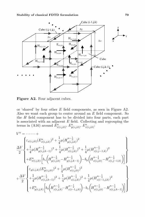
Therefore we seek an alternative method. We consider breakingthe right-hand side of (A15) into groups consisting of a few variables,with each group ideally also of quadratic form. Using Sylvester’sCriteria, conditions for each group to be positive definite are derivedand by combining the conditions from all group, a general criterioncan be obtained. This criterion is general in that if ∆x, ∆y, ∆z, ∆t,ε and µ of each cube fulfill the general criteria, the function V n onthe whole will be positive definite. The basis of choosing the groupis that we would like the positive definite criteria to hold when thereis variation of permittivity (or effective permittivity) ε(i,j,k) across themodel. Suppose we just pay particular attention to 4 cubes, whichare adjacent to each other, as shown in Figure A2. For simplicity weassume the model to be non-magnetic µ(i,j,k) = µ = µo and all cellsto be similar in size. Expanding (A15) and just concentrating on the
78 Kung and Chuah
stored energy in the 4 cubes of Figure A2.
V n =∆V2
{· · · · · ·+
∑r=x,y,z
(εr(i,j,k)(E
nr(i,j,k))
2 + 4 · 14µ(H
n− 12
r(i,j,k))2
)
−Hn− 12
x(i,j,k)
[by
(Enz(i,j+1,k)−Enz(i,j,k)
)− bz
(Eny(i,j,k+1)−Eny(i,j,k)
)]−Hn− 1
2
y(i,j,k)
[bz
(Enx(i,j,k+1)−Enx(i,j,k)
)− bx
(Enz(i+1,j,k)−Enz(i,j,k)
)]−Hn− 1
2
z(i,j,k)
[bx
(Eny(i+1,j,k)−Eny(i,j,k)
)− by
(Enx(i,j+1,k)−Enx(i,j,k)
)]+
∑r=x,y,z
(εr(i−1,j,k)(E
nr(i−1,j,k))
2 + 4 · 14µ(H
n− 12
r(i−1,j,k))2
)
−Hn− 12
x(i−1,j,k)
[by
(Enz(i−1,j+1,k)−Enz(i−1,j,k)
)−bz
(Eny(i−1,j,k+1)−Eny(i−1,j,k)
)]−Hn− 1
2
y(i−1,j,k)
[bz
(Enx(i−1,j,k+1)−Enx(i−1,j,k)
)− bx
(Enz(i,j,k)−Enz(i−1,j,k)
)]−Hn− 1
2
z(i−1,j,k)
[bx
(Eny(i,j,k)−Eny(i−1,j,k)
)− by
(Enx(i−1,j+1,k)−Enx(i−1,j,k)
)]+
∑r=x,y,z
(εr(i,j,k−1)(E
nr(i,j,k−1))
2 + 4 · 14µ(H
n− 12
r(i,j,k−1))2
)
−Hn− 12
x(i,j,k−1)
[by
(Enz(i,j+1,k−1)−Enz(i,j,k−1)
)−bz
(Eny(i,j,k)−Eny(i,j,k−1)
)]−Hn− 1
2
y(i,j,k−1)
[bz
(Enx(i,j,k)−Enx(i,j,k−1)
)− bx
(Enz(i+1,j,k−1)−Enz(i,j,k−1)
)]−Hn− 1
2
z(i,j,k−1)
[bx
(Eny(i+1,j,k−1)−Eny(i,j,k−1)
)−by
(Enx(i,j+1,k−1)−Enx(i,j,k−1)
)]+
∑r=x,y,z
(εr(i,j−1,k)(E
nr(i,j−1,k))
2 + 4 · 14µ(H
n− 12
r(i,j−1,k))2
)
−Hn− 12
x(i,j−1,k)
[by
(Enz(i,j,k)−Enz(i,j−1,k)
)−bz
(Eny(i,j−1,k+1)−Eny(i,j−1,k)
)]−Hn− 1
2
y(i,j−1,k)
[bz
(Enx(i,j−1,k+1)−Enx(i,j−1,k)
)−bx
(Enz(i+1,j−1,k)−Enz(i,j−1,k)
)]−Hn− 1
2
z(i,j−1,k)
[bx
(Eny(i+1,j−1,k)−Eny(i,j−1,k)
)− by
(Enx(i,j,k)−Enx(i,j−1,k)
)]+ · · · · · ·
}(A16)
In (A16), the justification for writing the H components as 4 ·14µ(H
n− 12
r(i,j,k))2, (r = x, y, z) is because each H component is surrounded
Stability of classical FDTD formulation 79
x
y
z
Ex(i,j,k)
Ey(i,j,k)
Ez(i,j,k)
Hz(i,j-1,k)Hz(i,j,k)
Hx(i,j-1,k)
Hy(i-1,j,k)
Hy(i,j,k)
Hx(i,j,k)
Hz(i-1,j,k)
Hy(i,j,k-1)Hx(i,j,k-1)
Cube (i,j-1,k)
Cube (i-1,j,k)
Cube (i,j,k-1)
Cube
x
y
z∆
∆
∆
Figure A2. Four adjacent cubes.
or ‘shared’ by four other E field components, as seen in Figure A2.Also we want each group to center around an E field component. Sothe H field component has to be divided into four parts, each partis associated with an adjacent E field. Collecting and regrouping theterms in (A16) around Enx(i,j,k), E
ny(i,j,k), E
nz(i,j,k):
V n = · · · · · ·+
∆V2
εx(i,j,k)(Enx(i,j,k))2 +
14µ(H
n− 12
y(i,j,k))2
+14µ(H
n− 12
y(i,j,k−1))2 +
14µ(H
n− 12
z(i,j,k))2 +
14µ(H
n− 12
z(i,j−1,k))2
+Enx(i,j,k)
[bz
(Hn− 1
2
y(i,j,k)−Hn− 1
2
y(i,j,k−1)
)−by
(Hn− 1
2
z(i,j,k)−Hn− 1
2
z(i,j−1,k)
)]
+∆V2
εy(i,j,k)(Eny(i,j,k))2 +
14µ(H
n− 12
x(i,j,k))2
+14µ(H
n− 12
x(i,j,k−1))2 +
14µ(H
n− 12
z(i,j,k))2 +
14µ(H
n− 12
z(i−1,j,k))2
+Eny(i,j,k)
[bx
(Hn− 1
2
z(i,j,k)−Hn− 1
2
z(i−1,j,k)
)−bz
(Hn− 1
2
x(i,j,k)−Hn− 1
2
x(i,j,k−1)
)]

80 Kung and Chuah
+∆V2
εz(i,j,k)(Enz(i,j,k))2 +
14µ(H
n− 12
x(i,j,k))2
+14µ(H
n− 12
x(i,j−1,k))2 +
14µ(H
n− 12
y(i,j,k))2 +
14µ(H
n− 12
y(i−1,j,k))2
+Enz(i,j,k)
[by
(Hn− 1
2
x(i,j,k)−Hn− 1
2
x(i,j−1,k)
)−bx
(Hn− 1
2
y(i,j,k)−Hn− 1
2
y(i−1,j,k)
)]
+ · · · (A17)
In writing (A17) some irrelevant terms from (A16) have been excluded.Each expression in the braces is a group. Call the first group V nxs sinceits associated E field is along x axis, s is an integer enumerating theE field index (i, j, k). Proceeding to group according to all E fields inthe model, (A17) can be written as:
V n = ∆V
(∑s
V nxs +∑s
V nys +∑s
V nzs
), s = 1, 2, 3, . . . (A18)
By showing that each V nxs, Vnys, V
nzs is positive definite, then V n is also
positive definite. Suppose we consider one of the groups centering onEz component. Writing this as:
Vz = εE21 +
14µH2
3 +14µH2
1 +14µH2
2 +14µH2
4
+E1[by(H3 −H1)− bx(H2 −H4)]
= [E1 H1 H2 H3 H4]T
ε −12by −1
2bx12by
12bx
−12by
14µ 0 0 0
−12bx 0 1
4µ 0 012by 0 0 1
4µ 012bx 0 0 0 1
4µ
E1
H1
H2
H3
H4
= xTAx (A19)
Equation (A19) is only applicable for interior cells, i.e., when the cellis not a boundary cell. In general to include boundary cells, the matrixA should be generalized as:
A =
ε −12by −1
2bx12by
12bx
−12by a2
1µ 0 0 0−1
2bx 0 a21µ 0 0
12by 0 0 a2
3µ 012bx 0 0 0 a2
4µ
(A20)
Stability of classical FDTD formulation 81
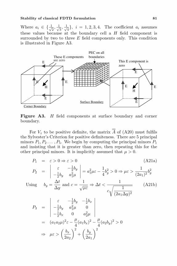
Where ai ∈ { 1√2, 1√
3, 1√
4}, i = 1, 2, 3, 4. The coefficient ai assumes
these values because at the boundary cell a H field component issurrounded by two to three E field components only. This conditionis illustrated in Figure A3.
E
H
E
E E
E
E E
E
H
These E componentsThis E component iszero
Corner BoundarySurface Boundary
PEC on allboundaries
are zero
Figure A3. H field components at surface boundary and cornerboundary.
For Vz to be positive definite, the matrix A of (A20) must fulfilsthe Sylvester’s Criterion for positive definiteness. There are 5 principalminors P1, P2 . . . , P5. We begin by computing the principal minors P1
and insisting that it is greater than zero, then repeating this for theother principal minors. It is implicitly assumed that µ > 0.
P1 = ε > 0⇒ ε > 0 (A21a)
P2 =
∣∣∣∣∣ ε −12by
−12by a2
1µ
∣∣∣∣∣ = a21µε−
14b2y > 0⇒ µε >
1(2a1)2
b2y
Using by =∆t∆y
and c =1√µε⇒ ∆t <
1
c
√1
(2a1∆y)2
(A21b)
P3 =
∣∣∣∣∣∣∣ε −1
2by −12bx
−12by a2
1µ 0−1
2bx 0 a22µ
∣∣∣∣∣∣∣= (a1a2µ)2ε−
µ
4(a1bx)2 −
µ
4(a2by)2 > 0
⇒ µε >
(bx2a2
)2
+(by2a1
)2
82 Kung and Chuah
⇒ ∆t <1
c
√1
(2a2∆x)2+
1(2a1∆y)2
(A21c)
P4 =
ε −12by −1
2bx12by
−12by a2
1µ 0 0−1
2bx 0 a22µ 0
12by 0 0 a2
3µ
= (−1)1+4
(12by
) ∣∣∣∣∣∣∣−1
2by a21µ 0
−12bx 0 a2
2µ12by 0 0
∣∣∣∣∣∣∣+ (−1)4+4a23µP3 > 0
⇒ −(a1a2
2µby
)2+
(a2
3µ)P3 > 0
⇒ µε >
(bx2a2
)2
+(by2a1
)2
+(by2a3
)2
⇒ ∆t <1
c
√√√√√√1
(2a2∆x)2+
1(2
a1a3√a2
1 + a23
)2
∆y2
(A21d)
P5 =
∣∣∣∣∣∣∣∣∣∣∣∣
ε −12by −1
2bx12by
12bx
−12by a2
1µ 0 0 0−1
2bx 0 a22µ 0 0
12by 0 0 a2
3µ 012bx 0 0 0 a2
4µ
∣∣∣∣∣∣∣∣∣∣∣∣
= (−1)1+5
(12bx
)∣∣∣∣∣∣∣∣∣
−12by a2
1µ 0 0−1
2bx 0 a22µ 0
12by 0 0 a2
3µ12bx 0 0 0
∣∣∣∣∣∣∣∣∣+(−1)5+5a2
4µP4 > 0
⇒ µε >
(bx2a2
)2
+(bx2a4
)2
+(by2a1
)2
+(by2a3
)2
⇒ ∆t <1
c
√√√√√√1(
2a2a4√a2
2 + a24
)2
∆x2
+1(
2a1a3√a2
1 + a23
)2
∆y2
(A21e)

Stability of classical FDTD formulation 83
Table A1. Computation of coefficient for ∆x and ∆y.
a1 or a2 a3 or a42a1a3√a21 + a23
or2a2a4√a22 + a24
ai i = 1, 2, 3, 4 2ai
1/√
4 1/√
4 1/√
2 ∼= 0.70711 1/√
4 2
1/√
4 1/√
3 1/√
7 ∼= 0.75593 1/√
3 2/√
3 ∼= 1.15470
1/√
4 1/√
2 2/√
6 ∼= 0.81650 1/√
2 2/√
2 ∼= 1.41421
1/√
3 1/√
3 2/√
6 ∼= 0.81650
1/√
3 1/√
2 2/√
5 ∼= 0.89443
1/√
2 1/√
2 1
From (A21a) to (A21e), we see that µ > 0, ε > 0 and ∆t needs to besmaller than a certain limit. The smallest limit from (A21b) to (A21e)for all combination of a1, a2, a3 and a4 will be taken as the constraintfor ∆t. Table A1 shows the values for the coefficient of ∆x and ∆y fordifferent combinations of a1, a2, a3 and a4.
Consider the expression:1√
1(c1∆x)2
+1
(c2∆y)2
=1√
1c21
(1
∆x2
)+
1c22
(1
∆y2
)
The smallest value is obtained when the denominator is maximum. If∆x and ∆y are fixed, then c1 and c2 must be as small as possible.Using Table A1, we observe that:
1√1
(2a1∆y)2
>1√
1(2a2∆x)2
+1
(2a1∆y)2
>1√√√√√
1(2a2∆x)2
+1(
2a1a3∆y√a1 + a3
)2
>1√√√√√√
1(2a2a4∆x√a2
2 + a42
)2 +1(
2a1a3∆y√a1 + a3
)2
(A22)
Also from Table A1, we observe that 2a1a3√a21+a23
and 2a2a4√a22+a24
are smallest
when a1 = a3 = a2 = a4 = 1√4. The corresponding coefficients for ∆x
84 Kung and Chuah
and ∆y are 1√2. We conclude that if ∆t satisfies:
∆t <1
c
√√√√√1(
1√2
)2
∆x2
+1(
1√2
)2
∆y2
=1
c√
2√
1∆x2
+1
∆y2
,
c =1√µε
(A23a)
Then all conditions of (A21b) to (A21e) will be fulfilled and Vz willbe positive definite. This procedure can also be applied to Vx and Vy,whose details would not be provided:
For Vx : ∆t <1
c√
2√
1∆y2
+1
∆z2
For Vy : ∆t <1
c√
2√
1∆x2
+1
∆z2(A23b)
Equations (A23a) and (A23b) apply to a single cell. To ensure that allgroups V nxs, V
nys and V nzs, s ∈ {1, 2, 3 . . . }, in the 3D model are positive
definite, these need to be enforced for every cell. This requirement canbe summarized as follows:
For a 3D FDTD model according to Yee’s formulation, supposethe followings apply:
1. Update equations for E and H field components are given by theCanonical FDTD Form (1a) to (1f).
2. Boundaries of the model are perfect electric conductor (PEC).3. All cubes are similar in size with edges ∆x, ∆y and ∆z.
Then for all i ∈ {1, 2, . . . , nx}, j ∈ {1, 2, . . . , ny}, k ∈ {1, 2, . . . , nz},∆V = ∆x∆y∆z, the function:
V n =∆V2
nz∑k=1
ny∑j=1
nx∑i=1
[ ∑r=x,y,z
(εr(i,j,k)(E
nr(i,j,k))
2 + µ(Hn− 1
2
r(i,j,k))2
)
− ∆t(Hn− 1
2 · ∇ × En)
(i,j,k)
]
is positive definite if and only if:
• εx(i,j,k) > 0, εy(i,j,k) > 0, εz(i,j,k) > 0 and µ > 0.
• For ε = min{εx(i,j,k), εy(i,j,k), εz(i,j,k)} and cm = 1√µε , let:

Stability of classical FDTD formulation 85
∆t < min
1
cm√
2√
1∆y2
+ 1∆z2
,1
cm√
2√
1∆x2 + 1
∆z2
,1
cm√
2√
1∆x2 + 1
∆y2
This proves Lemma 2.2.
APPENDIX B. STABILITY FOR 3D FDTD MODEL
We now prove Theorem 2.3. Suppose a FDTD framework satisfies allthe conditions of Lemma 2.1 and 2.2. Since V n is positive definite, itcan be written in the form [16]:
V n = XTP X, X ∈ RM (B1)
where M is as given by (5b) and P is a square symmetric matrix oforder M . Superscript T represents matrix transposition. Introducingthe linear transformation X = QY :
V n = YT
(QTP Q
)Y (B2)
The matrix transformation QTP Q of (B2) is a special form of
Similarity Transformation known as Congruence Transformation [16].Since matrix P is positive definite, from linear algebra we know thata nonsingular matrix Q exists such that [16, chapter 3]:
QTP Q = diag(1, 1, 1, . . . , 1)
Thus
V n = YT
(QTP Q
)Y = Y
TY = y2
1 + y22 + y2
3 + · · ·+ y2M (B3)
Taking an arbitrary norm for Y = Q−1X:
∥∥Y ∥∥ =∥∥∥∥Q−1
X
∥∥∥∥ ≤∥∥∥∥Q−1
∥∥∥∥∥∥X∥∥ (B4)
Where∥∥∥∥Q−1
∥∥∥∥ is a finite positive value called the matrix or operator
norm as defined in [16, chapter 2]. We thus have the followingimplication from (B4):∥∥Y ∥∥→∞⇒ ∥∥X∥∥→∞ (B5)
86 Kung and Chuah
Observe that from (B3), V n = XTP X = Y
TY is radially unbounded
[13, chapter 3] in relation to elements of Y . This means that ifV n approaches infinity, at least one of the elements of Y must alsoapproaches infinity. Suppose we use the L2 vector norm:∥∥X∥∥ =
(x2
1 + x22 + · · ·x2
M
) 12 and
∥∥Y ∥∥ =(y21 + y2
2 + · · ·+ y2M
) 12
(B6)
Using (B5) we note that V n is also radially unbounded in relation toelements of X. This implies that if V n is bounded, all the elements inX must also be finite, i.e., all the E and H field components are finite.For V n to be bounded for n = 1, 2, 3, . . . , a sufficient condition is Pdbe negative or zero. This completes the proof. ✷
APPENDIX C. NEGATIVE REGION FOR RESISTIVEVOLTAGE SOURCE
We first note from [2] that to derive equation (17) the current of aresistive voltage source is:
In+ 1
2s =
∆t2Rs
(Enz + En+1
z
)+Vn+ 1
2s
Rs(C1)
From ∇× H = J + ε∂E∂t and using center difference scheme accordingto Yee’s formulation [3], concentrating on z component of E field at(i, j, k) (assuming the source to coincide with Ez(i,j,k)):
∇×Hn+ 12
z(i,j,k) =In+ 1
2s
∆x∆y+ε
∆t
(En+1z(i,j,k) + Enz(i,j,k)
)(C2)
Let Vn+ 1
2s be a constant, called it Vso and limiting the maximum
source current to Is(max) = VsoRs
. Let us also introduce the notations
x = Enz(i,j,k), xn+1 = En+1
z(i,j,k), y = ∇ ×Hn+ 12
z(i,j,k), v = Vso∆z . Then from
(C2):
∆tε∇×Hn+ 1
2
z(i,j,k) −(En+1z(i,j,k) + Enz(i,j,k)
)
=∆tI
n+ 12
s
ε∆x∆y< 2
∆t∆z2ε∆x∆y∆z
· VsoRs
= 2Dzv
⇒ y <2ε∆tDzv +
ε
∆t(xn+1 − x
)(C3)
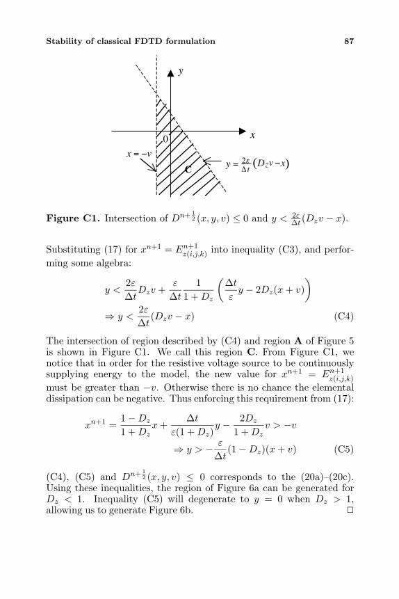
Stability of classical FDTD formulation 87
x
y
0
(yt
= ε2vx −=
C ∆Dzv −x (
Figure C1. Intersection of Dn+ 12 (x, y, v) ≤ 0 and y < 2ε
∆t(Dzv − x).
Substituting (17) for xn+1 = En+1z(i,j,k) into inequality (C3), and perfor-
ming some algebra:
y <2ε∆tDzv +
ε
∆t1
1 +Dz
(∆tεy − 2Dz(x+ v)
)
⇒ y <2ε∆t
(Dzv − x) (C4)
The intersection of region described by (C4) and region A of Figure 5is shown in Figure C1. We call this region C. From Figure C1, wenotice that in order for the resistive voltage source to be continuouslysupplying energy to the model, the new value for xn+1 = En+1
z(i,j,k)
must be greater than −v. Otherwise there is no chance the elementaldissipation can be negative. Thus enforcing this requirement from (17):
xn+1 =1−Dz
1 +Dzx+
∆tε(1 +Dz)
y − 2Dz
1 +Dzv > −v
⇒ y > − ε
∆t(1−Dz)(x+ v) (C5)
(C4), (C5) and Dn+ 12 (x, y, v) ≤ 0 corresponds to the (20a)–(20c).
Using these inequalities, the region of Figure 6a can be generated forDz < 1. Inequality (C5) will degenerate to y = 0 when Dz > 1,allowing us to generate Figure 6b. ✷

88 Kung and Chuah
REFERENCES
1. Yee, K. S., “Numerical solution of initial boundary value problemsinvolving Maxwell’s equations in isotropic media,” IEEE Trans.Antennas and Propagation, Vol. 14, 302–307, May 1966.
2. Piket-May, M. J., A. Taflove, and J. Baron, “FD-TD modeling ofdigital signal propagation in 3-D circuits with passive and activeloads,” IEEE Trans. Microwave Theory and Techniques, Vol. 42,1514–1523, August 1994.
3. Taflove, A., Computational Electrodynamics — The finite-difference time-domain method, Artech House, 1995.
4. Kung, F. and H. T. Chuah, “Modeling a diode in FDTD,” J. ofElectromagnetic Waves and Appl., Vol. 16, No. 1, 99–110, 2002.
5. Kung, F. and H. T. Chuah, “Modeling of bipolar junctiontransistor in FDTD simulation of printed circuit board,” Progressin Electromagnetic Research, PIER 36, 179–192, 2002.
6. Pereda, J. A., L. A. Vielva, A. Vegas, et al., “Analyzingthe stability of the FDTD technique by combining the vonNeumann method with the Routh-Hurwitz criterion,” IEEETrans. Microwave Theory and Techniques, Vol. 49, 377–381, Feb.2001.
7. Thiel, W. and L. P. B. Katehi, “Some aspects of stability andnumerical dissipation of the finite-difference time-domain (FDTD)technique including passive and active lumped-elements,” IEEETrans. Microwave Theory and Techniques, Vol. 50, 2159–2165,Sep. 2002.
8. Remis, R. F., “On the stability of the finite-difference time-domainmethod,” J. of Computational Physics, Vol. 163, No. 1, 249–261,Sep. 2000.
9. Strikwerda, J. C., Finite Difference Schemes and PartialDifferential Equations, Wadsworth & Brooks/Cole MathematicsSeries, 1989.
10. Scheinerman, E. R., Invitation to Dynamical Systems, PrenticeHall, 1996.
11. Elaydi, S. N., Discrete Chaos, Chapman & Hall/CRC, 2000.12. Merkin, D. R., Introduction to the Theory of Stability, Springer-
Verlag, 1997.13. Khalil, H. K., Nonlinear Systems, 2nd edition, Prentice Hall, 1996.14. James, G., Advance Modern Engineering Mathematics, Addison-
Wesley, 1993.15. “Surface mount RF Schottky barrier diodes: HSMS-

Stability of classical FDTD formulation 89
282x series,” Technical Data, Agilent Technologies Inc.,www.semiconductor.agilent.com, 2000.
16. Ortega, J. M., Matrix Theory — A second course, Plenum Press,1987.
Related Documents