03-Gravitational Search Algorithm Combined with Chaos for Unconstrained Numerical Optimization

Applied Mathematics and Computation 231 (2014) 48–62

Contents lists available at ScienceDirect

Applied Mathematics and Computation

journal homepage: www.elsevier .com/ locate /amc

Gravitational search algorithm combined with chaosfor unconstrained numerical optimization

0096-3003/$ - see front matter � 2014 Elsevier Inc. All rights reserved.http://dx.doi.org/10.1016/j.amc.2013.12.175

⇑ Corresponding author.E-mail address: [email protected] (S. Gao).

Shangce Gao a,⇑, Catherine Vairappan b, Yan Wang c, Qiping Cao d, Zheng Tang c

a College of Information Sciences and Technology, Donghua University, Shanghai 201620, Chinab Tateyama Institute of System, Toyama-shi 930-0016, Japanc Graduate School of Innovative Life Science, University of Toyama, Toyama-shi 930-8555, Japand School of Electrical and Computer Engineering, Kanazawa University, Kanazawa-shi 920-1192, Japan

a r t i c l e i n f o a b s t r a c t

Keywords:Gravitational search algorithmChaosLocal searchPerformanceParticle swarm optimization

Gravitational search algorithm (GSA) is the one of the newest developed nature-inspiredheuristics for optimization problem. It is designed based on the Newtonian gravity andhas shown excellent search abilities when applying it to optimization problems. Neverthe-less, GSA still has some disadvantages such as slow convergence speed and local optimatrapping problems. To alleviate these inherent drawbacks and enhance the performanceof GSA, chaos, which is of ergodicity and stochasticity, is incorporated into GSA by twokinds of methods. One method uses chaos to generate chaotic sequences to substitute ran-dom sequences, while another one uses chaos to act as a local search approach. The resul-tant hybrid algorithms, called chaotic gravitation search algorithms (CGSA1 and CGSA2),thus reasonably have advantages of both GSA and chaos. Eight widely used benchmarknumerical optimization problems are chosen from the literature as the test suit. Experi-mental results demonstrate that both CGSA1 and CGSA2 perform better than GSA andother five chaotic particle swarm optimization.

� 2014 Elsevier Inc. All rights reserved.

1. Introduction

Many problems arising from diverse areas such as network design for optimal performance, production-planning, inven-tory, and facility location can be formulated as combinatorial optimization problems. While many of these problems can besolved in polynomial time, a majority belong to the class of NP-hard [1]. In order to deal with these hard combinatorial opti-mization problems, approximation and heuristic algorithms have been employed as a compromise between solution qualityand computational time. This makes heuristic algorithms well-suited for applications where computational resources arelimited. The success of these heuristic algorithms depends on the computational complexity of the algorithm and their abil-ity to converge to the optimal solution [2]. In most cases, the solutions obtained by these heuristic algorithms are not guar-anteed optimal.

A recently developed class of heuristic algorithms, known as the meta-heuristic algorithms, have demonstrated promis-ing results in the field of combinatorial optimization. Meta-heuristic algorithms represent the class of all-purpose searchtechniques that can be applied to a variety of optimization problems including combinatorial optimization. The class ofmeta-heuristic algorithms include (but not restricted to) simulated annealing [3], tabu search, evolutionary algorithms(including genetic algorithms), ant colony optimization [4], bacterial foraging [5], scatter search, iterated local search, hill

S. Gao et al. / Applied Mathematics and Computation 231 (2014) 48–62 49

climbing [6], particle swarm optimization (PSO) [7], and so on. These algorithms solve different optimization problems. Somealgorithms give a better solution for some particular problems than others. Nevertheless, there is no specific algorithm toachieve the best solution for all optimization problems. Hence, searching for new heuristic optimization algorithms is anopen problem [8].

More recently, a new family of computationally efficient meta-heuristic algorithms better posed at handling non-convexsolution spaces has been developed. From this family of meta-heuristic algorithms, is gravitational search algorithm (GSA)[9]. Like other physics-inspired meta-heuristic algorithms, GSA is an adaptive search technique which is based on the New-tonian gravity. In GSA, a population of candidate solutions are modeled as a swarm of objects. At each iteration, the objectsupdate their position (and solution) by moving stochastically towards regions previously visited by the other objects. Theobject with heavier mass has a larger effective attraction radius and hence a greater intensity of attraction. By lapse of time,the objects tend to move towards the heaviest object. The simplicity, robustness, and adaptability of GSA, enable it to haveapplications in a wide-range of function optimization problems [9,10], and some real-world problems [11–14]. In compar-ison with other well-known optimization algorithms, such as PSO, GSA has been confirmed higher performance in searchingability. However, GSA still has some inherent disadvantages, such as it usually sticks on local optimal solutions, which indi-cates that it is unable to improve the solutions’ quality in the latter search phases.

Hybridization is nowadays recognized to be an essential aspect of high performing algorithms. Pure algorithms are almostalways inferior to hybridizations [15]. Numerous algorithms like evolution-neural network, simulated annealing-evolution,chaos-neural network and so forth have been brought up for discussion, meanwhile successfully applied. Among these newlyemerged algorithms, chaos [16], which is a universal phenomenon of nonlinear dynamic systems, is regarded as a powerfultool for hybridization and has recently received much interest. Chaos is apparently an irregular motion, seemingly unpredict-able random behavior exhibited by a deterministic nonlinear system under deterministic conditions. Chaotic variables cango through every state in a certain area according to their own regularity without repetition. Due to the ergodic and dynamicproperties of chaos variables, chaos search is more capable of hill-climbing and escaping from local optima than randomsearch [17], and thus has been applied to the area of optimization computation. In the last two decades, various chaos-basedoptimization algorithms, for example, a chaos optimization algorithm (COA) [18], a chaos-based simulated annealing algo-rithm (CSA) [19], a hybrid chaotic ant swarm optimization [20], chaotic harmony search algorithms (CHS) [21], chaotic beecolony algorithms (CABC) [22] and chaotic particle swarm optimization algorithms (CPSO) [23–26], have been proposed forsolving complex optimization problems more efficiently.

Following this consideration, in this paper, we propose a chaotic gravitational search algorithm (CGSA) which combinesGSA with chaos. There are two methods to incorporate chaos into GSA: (1) One method is to use sequences generated bychaotic systems to substitute random numbers for different parameters of GSA where it is necessary to make a random-based choice. By this way, it is intended to enhance the global convergence and to prevent the search to stick on a local solu-tion. (2) The other method is to insert the chaotic search as a local search approach into the procedures of GSA. The archi-tecture of the hybrid algorithm is emerged by switching the chaotic search and GSA to each other according to certainconditions. By doing so, the chaotic search will directly improve the current solutions found by GSA, leading a faster conver-gence speed, and further giving a higher probability to jump out of local optima. As a result, based on the above two methodswe construct two types of chaotic gravitational search algorithms, called CGSA1 and CGSA2, respectively, aiming not only toimprove the performance of the traditional GSA, but also to find out which embedded method is better.

The remainder of this paper is organized as follows: in the next section, we provide a general description of the gravita-tional search algorithm. In Section 3, the chaotic gravitational search algorithms CGSA1 and CGSA2 are proposed, respec-tively. In Section 4, we validate the two hybrid algorithms by applying them to a number of unconstrained numericaloptimization functions. Finally we give some general remarks to conclude this paper.

2. Traditional gravitational search algorithm

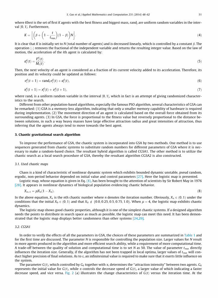
Gravitational search algorithm is a meta-heuristic technique inspired by physical behavior among individuals. GSA isoriginally presented by Rashedi et al. [9] for optimizing continuous nonlinear functions in 2009. The algorithm is basedon the Newtonian gravity: ‘‘Every particle in the universe attracts every other particle with a force that is directly propor-tional to the product of their masses and inversely proportional to the square of the distance between them.’’ Fig. 1 depictsthe conceptual graph of the law of gravity. In GSA, agents are considered as objects and their performance is measured bytheir masses. Each agent in GSA has four specifications: position, inertial mass, active gravitational mass, and passive grav-itational mass. The position of agent corresponds to a solution of the optimization problem at hand. Moving the position ofagent can result in an improvement of the solution’s quality. It is worth pointing out that, although gravitational and inertiamasses have different physical meanings, they are assumed to be equivalent during computation. All masses are calculatedby using the map of fitness.

From a view of optimization context, GSA approach can be regarded as a population-based algorithm that performs a par-allel search on the space of solutions. Several solutions of a given problem constitute a population (the swarm). Each solutionis seen as an object. All objects attract each other by a gravity force, and this force causes a movement of all objects globallytowards the objects with heavier masses. The heavy masses correspond to good solutions of the problem. These objectssearch the problem’s solution space by balancing the intensification and the diversification efforts. By lapse of time, the

FiQ

Fij

Fi2

Fi1

Fig. 1. Gravitational force: every agent (mass) accelerates towards the resulting force that act on it from the other agents.

50 S. Gao et al. / Applied Mathematics and Computation 231 (2014) 48–62

objects will be attracted by the heaviest object, which presents an optimum solution in the search space. The process iteratesuntil a stopping condition is fulfilled.

The flowchart of GSA is illustrated in Algorithm 1. Assumed there are N agents, the position of the ith agent isXi ¼ ðx1

i ; . . . ; xdi ; . . . ; xn

i Þ, where xdi presents the position of ith agent in the dth dimension. In Algorithm 1, the initialization pro-

cess is from line 1 to line 3, generating the initial population of agents randomly. The optimization process which starts fromline 4 to line 11 is an iteration-based searching algorithm based on Newton gravitation theory. The force acting on the ithagent from the jth agent is defined as:

FdijðtÞ ¼ GðtÞMiðtÞ �MjðtÞ

RijðtÞ þ eðxd

j ðtÞ � xdi ðtÞÞ; ð1Þ

where, Mi and Mj are masses of agents. Mi is calculated through the map of fitness Mi ¼ fitiðtÞ�worstðtÞbestðtÞ�worstðtÞ, where bestðtÞ is the best

fitness of all agents, worstðtÞ is the worst fitness of all agents, and fitiðtÞ represents the fitness of agent Mi by calculating theobjective function. Besides, Euclidean distance between two agents is computed RijðtÞ ¼ kxiðtÞ; xjðtÞk2, and e is a small con-stant, preventing the denominator in Eq. (1) from being zero. In addition, GðtÞ is the gravitational constant at time t. A pointworth emphasizing is that GðtÞ is very important in determining the performance of GSA. It is defined by a function of theiteration time t:

Algorithm 1. (Traditional GSA)

01: for all agent i (i ¼ 1;2; . . . ;N) do02: initialize position xi randomly in search space03: end-for04: while termination criteria not satisfied do05: for all agent i do

06: compute overall force Fdi ðtÞ according to Eqs. (1)–(4)

07: compute acceleration adi ðtÞ according to Eq. (5)

08: update velocity according to Eq. (6)09: update position according to Eq. (7)10: end-for11: end-while

GðtÞ ¼ G0 exp �at

tmax

� �; ð2Þ

where G0 is the initial value, a is a shrinking constant, t is the current iteration number, tmax is the maximum number of iter-ations. For the ith agent, the overall force that acts on it is a randomly weighted sum of the forces exerted from the surround-ing agents.

Fdi ðtÞ ¼

Xj2Kbest;j–i

randjFdijðtÞ; ð3Þ

S. Gao et al. / Applied Mathematics and Computation 231 (2014) 48–62 51

where Kbest is the set of first K agents with the best fitness and biggest mass, randj are uniform random variables in the inter-val ½0;1�. Furthermore,

K ¼ bþ 1� ttmax

� �ð1� bÞ

� �N

� �: ð4Þ

It is clear that K is initially set to N (total number of agents) and is decreased linearly, which is controlled by a constant b. Theoperation b�c removes the fractional of the independent variable and returns the resulting integer value. Based on the law ofmotion, the acceleration of the ith agent is calculated by:

adi ðtÞ ¼

Fdi ðtÞ

MiðtÞ: ð5Þ

Then, the next velocity of an agent is considered as a fraction of its current velocity added to its acceleration. Therefore, itsposition and its velocity could be updated as follows:

vdi ðt þ 1Þ ¼ randivd

i ðtÞ þ adi ðtÞ; ð6Þ

xdi ðt þ 1Þ ¼ xd

i ðtÞ þ vdi ðt þ 1Þ; ð7Þ

where randi is a uniform random variable in the interval ½0;1�, which in fact is an attempt of giving randomized character-istics to the search.

Different from other population-based algorithms, especially the famous PSO algorithm, several characteristics of GSA canbe remarked: (1) GSA is a memory-less algorithm, indicating that only a smaller memory capability of hardware is requiredduring implementation. (2) The movement direction of an agent is calculated based on the overall force obtained from itssurrounding agents. (3) In GSA, the force is proportional to the fitness value but reversely proportional to the distance be-tween solutions, in such a way heavy masses have large effective attraction radius and great intensities of attraction, thusinferring that the agents always tend to move towards the best agent.

3. Chaotic gravitational search algorithm

To improve the performance of GSA, the chaotic system is incorporated into GSA by two methods. One method is to usesequences generated from chaotic systems to substitute random numbers for different parameters of GSA where it is nec-essary to make a random-based choice. The resultant hybrid algorithm is called CGSA1. The other method is to utilize thechaotic search as a local search procedure of GSA, thereby the resultant algorithm CGSA2 is also constructed.

3.1. Used chaotic maps

Chaos is a kind of characteristic of nonlinear dynamic system which exhibits bounded dynamic unstable, pseud random,ergodic, non-period behavior depended on initial value and control parameters [27]. Here the logistic map is presented.

Logistic map, whose equation is given in Eq. (8), has been brought to the attention of scientists by Sir Robert May in 1976[28]. It appears in nonlinear dynamics of biological population evidencing chaotic behavior.

Xnþ1 ¼ lXnð1� XnÞ: ð8Þ

In the above equation, Xn is the nth chaotic number where n denotes the iteration number. Obviously, Xn 2 ð0;1Þ under theconditions that the initial X0 2 ð0;1Þ and that X0 R f0:0;0:25;0:5;0:75;1:0g. When l ¼ 4, the logistic map exhibits chaoticdynamics.

The logistic map shows good chaotic properties, although it is one of the simplest chaotic systems. If a designed algorithmneeds the points to distribute in search space as much as possible, the logistic map can meet this need. It has been demon-strated that the logistic map displays better randomness than other systems [24,29].

3.2. CGSA1

In order to verify the effects of all the parameters in GSA, the choices of these parameters are summarized in Table 1 andfor the first time are discussed. The parameter N is responsible for controlling the population size. Larger values for N resultin more agents produced in the algorithm and more efficient search ability, while a requirement of more computational time.A trade-off between the quality of solution and computational time is to set N as 50. The value of parameter tmax directlyinfluences the iteration size. Generally, if the algorithm has not been trapped in local optima, larger values of tmax will con-duct higher precision of final solutions. As to e, an infinitesimal value is required to make sure that it exerts little influence onthe system.

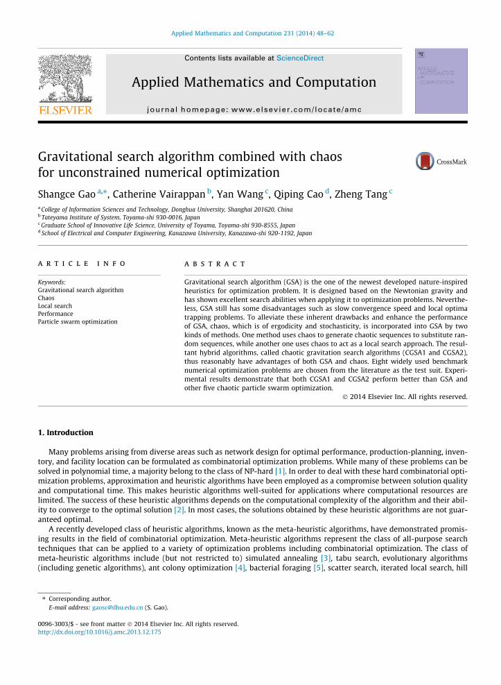
The parameter GðtÞ, which controlled by G0 together with a, determines the ‘‘attraction intensity’’ between two agents. G0

represents the initial value for GðtÞ, while a controls the decrease speed of GðtÞ, a larger value of which indicating a fasterdecrease speed, and vice versa. Fig. 2 (a) illustrates the change characteristics of GðtÞ versus the iteration time. At the

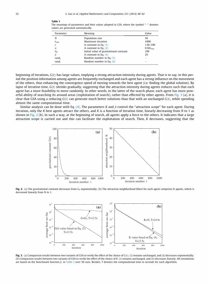
Table 1The meanings of parameters and their values adopted in GSA, where the symbol ‘‘�’’ denotesvalues are generated automatically.

Parameter Meaning Value

N Population size 50tmax Maximum iteration 1000e A constant in Eq. (1) 1.0e-100a A constant in Eq. (2) 0:02tmax

G0 Initial value of gravitational constant 100b A constant in Eq. (4) 2%randj Random number in Eq. (3) �randi Random number in Eq. (6) �

52 S. Gao et al. / Applied Mathematics and Computation 231 (2014) 48–62

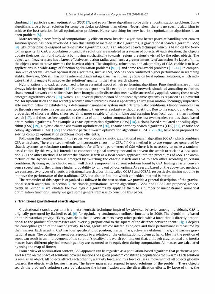
beginning of iterations, GðtÞ has large values, implying a strong attraction intensity during agents. That is to say, in this per-iod the position information among agents are frequently exchanged and each agent has a strong influence on the movementof the others, thus enhancing the convergence speed of moving towards the best agent (i.e. finding the global solution). Bylapse of iteration time, GðtÞ shrinks gradually, suggesting that the attraction intensity during agents reduces such that eachagent has a more feasibility to move randomly. In other words, in the latter of the search phase, each agent has more pow-erful ability of searching its around areas (exploitation of search), rather than effected by other agents. From Fig. 3 (a), it isclear that GSA using a reducing GðtÞ can generate much better solutions than that with an unchanged GðtÞ, while spendingalmost the same computational time.

Similar analysis can be done with Eq. (4). The parameters K and b control the ‘‘attraction scope’’ for each agent. Duringiteration, only the K best agents attract the others, and K is a function of iteration time, linearly decreasing from N to 1 asshown in Fig. 2 (b). In such a way, at the beginning of search, all agents apply a force to the others. It indicates that a largeattraction scope is carried out and this can facilitate the exploitation of search. Then, K decreases, suggesting that the

0 200 400 600 800 10000

20

40

60

80

100

iteration number: t

grav

itatio

nal c

onst

ant:

G(t

)

0 200 400 600 800 10000

10

20

30

40

50

iteration number: t

attr

actio

n ne

ighb

ourh

ood:

K

(a) (b)

Fig. 2. (a) The gravitational constant decreases from G0 exponentially; (b) The attraction neighborhood Kbest for each agent comprises K agents, which isdecreased linearly from N to 1.

0 200 400 600 800 100010

−20

10−15

10−10

10−5

100

105

iteration

ave

rage

bes

t−so

−fa

r

G(t) varies based on Eq. (2), T=13.5s

G=G0, T=13.5s

0 200 400 600 800 100010

−20

10−15

10−10

10−5

100

105

iteration

ave

rage

bes

t−so

−fa

r

K varies based on Eq. (4), T=13.5s

K=N, T=24.9s

(a) (b)

Fig. 3. (a) Comparison results between two variants of GSA to verify the effect of the choice of GðtÞ: (i) remains unchanged, and (ii) decreases exponentially;(b) Comparison results between two variants of GSA to verify the effect of the choice of K: (i) remains unchanged, and (ii) decreases linearly. All simulationsare based on the benchmark function f1 in Table 2 over 30 runs. Besides, T denotes the computational time in seconds for each algorithm.

S. Gao et al. / Applied Mathematics and Computation 231 (2014) 48–62 53

exploration fades out and exploitation fades in. At the end of search, there will be just one agent applying force to the others,making all the other agents move towards the current best one. In Fig. 3 (b), the comparison results between the two choicesof K demonstrate the superiority of the usage of Eq. (4), in terms of solution quality and computational time.

Based on the analysis concerning the above parameters, it is evident that there is no necessary to make a random-basedchoice for these parameters because there are some fixed rules of the choice to follow. Nevertheless, there are two random-based parameters randi and randj in GSA, representing the inertia weight value of velocity (in Eq. (6)) and the weight of com-ponents of the overall force (in Eq. (3)), respectively. The usage of the inertia weight randi in GSA is similar to that in PSO [7].In PSO, the value of inertia weight is a key factor to affect the convergence of algorithms [30]. A larger inertia weight achievesthe global exploration and a smaller inertia weight tends to facilitate the local exploration to fine-tune the current searcharea [31]. A point worth emphasizing is that although there are various methods to improve the inertia weight, such as atime-increasing function in [32,33], a dynamic scheme [34], a fuzzy variable adaption [35], and uniformly distribute randomnumbers [36,37], the chaotic system embedded method is undoubtedly a promising research direction [23,38]. Tracking theresearch history about the inertia weight in PSO, it is natural to incorporate chaotic system for determining the inertiaweight value into GSA, intending to improve its performance. As for the weight randj, whose effect is similar to the socialparameter (referring to [26] for a comprehensive description) in PSO, the analysis goes in a similar way. As a result, for bothrandi and randj whose values are randomly generated in the interval ½0;1� and unable to ensure the optimization’s ergodicityentirely in seach space, we use sequences chaosi and chaosj generated by the logistic map in Section 3.1 to substitute randi

and randj, respectively.Therefore, Eqs. (3) and (6) can be rewritten as:

Fdi ðtÞ ¼

Xj2Kbest;j–i

chaosjFdijðtÞ; ð9Þ

vdi ðt þ 1Þ ¼ chaosivd

i ðtÞ þ adi ðtÞ; ð10Þ

where both chaosi and chaosj are generated based on Eq. (8) and their initial values (i.e. chaosið0Þ and chaosjð0Þ) are randomlygenerated in ð0;1Þ and satisfy the conditions of feasibility in Eq. (8).

In addition, it is worth pointing out that the initialization process of GSA can also be accomplished chaotically, rather thanrandomly. That is to say, the positions of all N agents: Xi ¼ ðx1

i ; . . . ; xdi ; . . . ; xn

i Þ; i ¼ 1;2; . . . ;N are generated chaotically by thefollowing logistic mappings.

xdiþ1 ¼ lxd

i ð1� xdi Þ; i ¼ 1;2; . . . ;N; d ¼ 1;2; . . . ;n; ð11Þ

where i is the serial number of agents, d denotes the dimension of the position of each agent, l ¼ 4. Let i ¼ 0, and given the nchaotic variables different initial values xd

0 ðd ¼ 1;2; . . . ;nÞ, then the values of the n chaotic variables xd1 ðd ¼ 1;2; . . . ;nÞ are

produced by the logistic equation and encoded into a real-coded position of agent, i.e. X1 ¼ ðx11; x

21; . . . ; xn

1Þ. Letj ¼ 1;2; . . . ;N � 1, and then other N � 1 positions of agents are produced by the same method.

From the above construction method, it can be easily find out that the range of chaotic variables in each position is ½0;1�,which maybe different from that of optimization variables. Therefore, the ‘‘solution space transformation’’ between chaoticvariables and optimization variables must be determined using the following method. The ergodic space of the chaos system(11) is mapped to the solution space of the optimization problem by Eq. (12), and thus the n optimization variables can beexpressed by the n chaotic variables.

xdi ¼ xd

min þ ðxdmax � xd

minÞxdi ; d ¼ 1;2; . . . ;n; ð12Þ

where xdmin and xd

max are the search boundaries of X, supposing Xmin ¼ ðx1min; x

2min; . . . ; xn

minÞ and Xmax ¼ ðx1max; x

2max; . . . ; xn

maxÞ, thusthe domain of the optimization function is ½Xmin;Xmax�n. By doing so, it is intended to place the N initial agents in the searchspace ergodically.

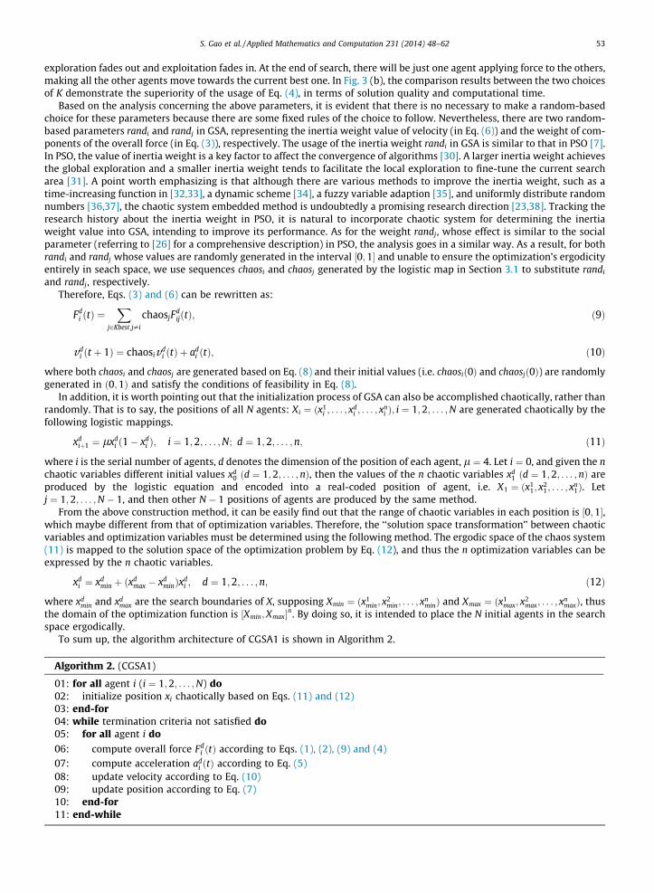
To sum up, the algorithm architecture of CGSA1 is shown in Algorithm 2.

Algorithm 2. (CGSA1)

01: for all agent i (i ¼ 1;2; . . . ;N) do02: initialize position xi chaotically based on Eqs. (11) and (12)03: end-for04: while termination criteria not satisfied do05: for all agent i do

06: compute overall force Fdi ðtÞ according to Eqs. (1), (2), (9) and (4)

07: compute acceleration adi ðtÞ according to Eq. (5)

08: update velocity according to Eq. (10)09: update position according to Eq. (7)10: end-for11: end-while

3.3. CGSA2

54 S. Gao et al. / Applied Mathematics and Computation 231 (2014) 48–62

Compared with CGSA1, CGSA2 does not change any values of the parameters in GSA, but incorporates the chaotic systemas a local search approach into GSA. Algorithm 3 illustrates the flowchart of CGSA2.

In Algorithm 3, lines 11–13 state the procedures of the proposed chaotic local search, while the other codes representtraditional GSA procedures. In detail, line 11 finds out the current global best agent Xg ¼ ðx1

g ; x2g ; . . . ; xn

gÞ, line 12 implementsthe chaotic local search (CLS) algorithm, and line 13 decreases chaotic search radius for the purpose of making CLS moreefficiently.

Algorithm 3. (CGSA2)

01: for all agent i (i ¼ 1;2; . . . ;N) do02: initialize position xi randomly in search space03: end-for04: while termination criteria not satisfied do05: for all agent i do

06: compute overall force Fdi ðtÞ according to Eqs. (1)–(4)

07: compute acceleration adi ðtÞ according to Eq. (5)

08: update velocity according to Eq. (6)09: update position according to Eq. (7)10: end-for11: find out the global best agent Xg

12: implement chaotic local search approach (CLS)13: decrease chaotic search radius using Eq. (16)14: end-while

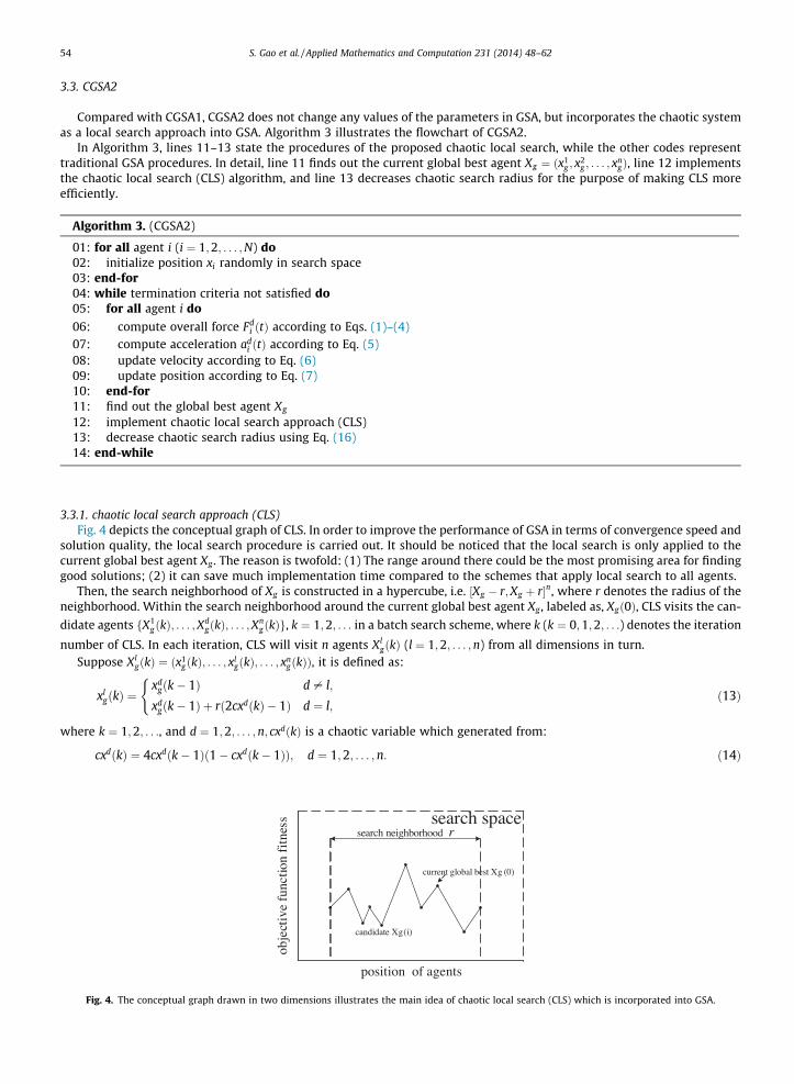
3.3.1. chaotic local search approach (CLS)Fig. 4 depicts the conceptual graph of CLS. In order to improve the performance of GSA in terms of convergence speed and

solution quality, the local search procedure is carried out. It should be noticed that the local search is only applied to thecurrent global best agent Xg . The reason is twofold: (1) The range around there could be the most promising area for findinggood solutions; (2) it can save much implementation time compared to the schemes that apply local search to all agents.

Then, the search neighborhood of Xg is constructed in a hypercube, i.e. ½Xg � r;Xg þ r�n, where r denotes the radius of theneighborhood. Within the search neighborhood around the current global best agent Xg , labeled as, Xgð0Þ, CLS visits the can-

didate agents fX1gðkÞ; . . . ;Xd

gðkÞ; . . . ;XngðkÞg, k ¼ 1;2; . . . in a batch search scheme, where k (k ¼ 0;1;2; . . .) denotes the iteration

number of CLS. In each iteration, CLS will visit n agents XlgðkÞ (l ¼ 1;2; . . . ;n) from all dimensions in turn.

Suppose XlgðkÞ ¼ ðx1

gðkÞ; . . . ; xlgðkÞ; . . . ; xn

gðkÞÞ, it is defined as:

F

xlgðkÞ ¼

xdgðk� 1Þ d – l;

xdgðk� 1Þ þ rð2cxdðkÞ � 1Þ d ¼ l;

(ð13Þ

where k ¼ 1;2; . . ., and d ¼ 1;2; . . . ;n; cxdðkÞ is a chaotic variable which generated from:

cxdðkÞ ¼ 4cxdðk� 1Þð1� cxdðk� 1ÞÞ; d ¼ 1;2; . . . ;n: ð14Þ

position of agents

current global best Xg (0)

ssentifnoitcnuf

evitcejbo

search spacesearch neighborhood r

candidate Xg(i)

ig. 4. The conceptual graph drawn in two dimensions illustrates the main idea of chaotic local search (CLS) which is incorporated into GSA.

S. Gao et al. / Applied Mathematics and Computation 231 (2014) 48–62 55

It should be noticed that if the acquired values of xlgðkÞ in Eq. (13) locate out of the search neighborhood ½Xg � r;Xg þ r�n, these

values will be resetted to the closest boundary values.After each iteration, the best agent during the batch will be picked up. Without loss of generality, for a minimization opti-

mization problem,

XgðkÞ ¼ MINfX1gðkÞ; . . . ;Xd

gðkÞ; . . . ;XngðkÞg; ð15Þ

where MIN returns the one whose objective function fitness is the minimal.The above processes cycle until a better solution XgðkÞ than the current global best solution Xgð0Þ is found, or the max-

imum iteration number kmax is reached. If a better solution XgðkÞ is found, output it as the result of CLS, and say that theimplementation of CLS is successful; otherwise just output Xgð0Þ. Algorithm 4 briefly summarizes the flowchart of CLS.

Algorithm 4. (CLS)

01: for all dimension d (d ¼ 1;2; . . . ;n) do02: initialize chaotic variables cxdð0Þ ¼ randð0;1Þ03: end-for04: while termination criteria not satisfied do05: for all dimension d do

06: compute candidate XdgðkÞ using Eqs. (13) and (14)

07: end-for08: pick up local optimal XgðkÞ using Eq. (15)09: end-while

In addition, by the fact that chaotic search is efficient in small range [18,24,25], Eq. (16) is used to narrow the searchneighborhood of CLS by lapse of iteration in order to improve its searching efficiency.

r ¼ qr; ð16Þ

where q is a shrinking parameter. Initially, the search radius is set to be half of the search domain, i.e., r0 ¼ 12 ðXmax � XminÞ.

3.3.2. general remarks

(1) First and foremost, the usage of CLS definitely enhances the local search ability of GSA, especially the most promisingareas round the current global best agent are exploited.

(2) Besides, when exploiting the neighborhood of the current global best agent, all candidate agents are generated by achaotic methodology. Taking the advantages of ergodicity and dynamics of chaos variables, CLS can exploit the neigh-borhood efficiently.

(3) Furthermore, the more successful iterations of CLS, the faster convergence speed of the algorithm. The reason is thatnot only the current global best agent is improved, but also the other agents can also be improved due to the attractionof the best one, thus inferring a comprehensive improvement for all agents.

(4) Last but not least, the gradually narrowed neighborhood radius guarantees the efficiency of CLS in the latter searchingphases of the algorithm.

4. Experiments and discussions

4.1. Numerical problem formulation

The problem of finding the global minimum of a real-valued function f ðXÞ in n-dimensional search space S is denoted by

min f ðXÞ;s:t: X 2 S # Rn;

ð17Þ

where f ðXÞ may be nonlinear, non-convex and non-differential. A vector X� 2 S ¼ ½Xmin;Xmax�n satisfying f ðX�Þ 6 f ðXÞ for allX 2 S is called a global minimizer of f ðXÞ over S and the corresponding value f ðX�Þ is called a global minimum.

4.2. Benchmark functions

To illustrate the effectiveness and performance of CGSA1 and CGSA2 for numerical optimization problems, a set of 8 rep-resentative benchmark functions is employed to evaluate them and then make a comparison with the standard GSA.

Table 2 summarizes the name, definition, dimension of search space, search domain, global minimum fitness, and prop-erty of these functions. The dimension for all functions are set at a relatively large value 30. All tested functions have a global

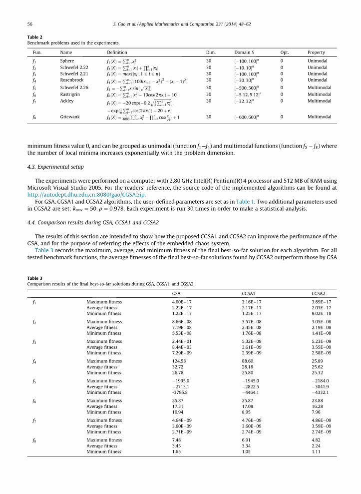
Table 2Benchmark problems used in the experiments.

Fun. Name Definition Dim. Domain S Opt. Property

f1 Sphere f1ðXÞ ¼Pn

i¼1x2i

30 ½�100;100�n 0 Unimodal

f2 Schwefel 2.22 f2ðXÞ ¼Pn

i¼1jxij þQn

i¼1jxij 30 ½�10;10�n 0 Unimodalf3 Schwefel 2.21 f3ðXÞ ¼ maxfjxij;1 6 i 6 ng 30 ½�100;100�n 0 Unimodalf4 Rosenbrock f4ðXÞ ¼

Pn�1i¼1 ½100ðxiþ1 � x2

i Þ2 þ ðxi � 1Þ2� 30 ½�30;30�n 0 Unimodal

f5 Schwefel 2.26 f5 ¼ �Pn

i¼1xisinðffiffiffiffiffiffiffijxij

pÞ 30 ½�500;500�n 0 Multimodal

f6 Rastrigrin f6ðXÞ ¼Pn

i¼1½x2i � 10cosð2pxiÞ þ 10� 30 ½�5:12;5:12�n 0 Multimodal

f7 Ackley f7ðXÞ ¼ �20 expð�0:2ffiffiffiffiffiffiffiffiffiffiffiffiffiffiffiffiffiffiffi1n

Pni¼1x2

i

qÞ 30 ½�32;32�n 0 Multimodal

� expð1nPn

i¼1cosð2pxiÞÞ þ 20þ ef8 Griewank f8ðXÞ ¼ 1

4000

Pni¼1x2

i �Qn

i¼1cosð xiffiip Þ þ 1 30 ½�600;600�n 0 Multimodal

56 S. Gao et al. / Applied Mathematics and Computation 231 (2014) 48–62

minimum fitness value 0, and can be grouped as unimodal (function f1—f4) and multimodal functions (function f5 � f8) wherethe number of local minima increases exponentially with the problem dimension.

4.3. Experimental setup

The experiments were performed on a computer with 2.80 GHz Intel(R) Pentium(R) 4 processor and 512 MB of RAM usingMicrosoft Visual Studio 2005. For the readers’ reference, the source code of the implemented algorithms can be found athttp://autodept.dhu.edu.cn:8080/gao/CGSA.zip.

For GSA, CGSA1 and CGSA2 algorithms, the user-defined parameters are set as in Table 1. Two additional parameters usedin CGSA2 are set: kmax ¼ 50;q ¼ 0:978. Each experiment is run 30 times in order to make a statistical analysis.

4.4. Comparison results during GSA, CGSA1 and CGSA2

The results of this section are intended to show how the proposed CGSA1 and CGSA2 can improve the performance of theGSA, and for the purpose of referring the effects of the embedded chaos system.

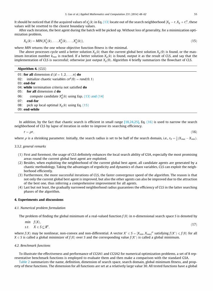
Table 3 records the maximum, average, and minimum fitness of the final best-so-far solution for each algorithm. For alltested benchmark functions, the average fitnesses of the final best-so-far solutions found by CGSA2 outperform those by GSA

Table 3Comparison results of the final best-so-far solutions during GSA, CGSA1, and CGSA2.

GSA CGSA1 CGSA2

f1 Maximum fitness 4.00E�17 3.16E�17 3.89E�17Average fitness 2.22E�17 2.17E�17 2.03E�17Minimum fitness 1.22E�17 1.25E�17 9.02E�18

f2 Maximum fitness 8.66E�08 3.57E�08 3.05E�08Average fitness 7.19E�08 2.45E�08 2.19E�08Minimum fitness 5.53E�08 1.76E�08 1.41E�08

f3 Maximum fitness 2.44E�01 5.32E�09 5.23E�09Average fitness 8.44E�03 3.61E�09 3.55E�09Minimum fitness 7.29E�09 2.39E�09 2.58E�09

f4 Maximum fitness 124.58 88.60 25.89Average fitness 32.72 28.18 25.62Minimum fitness 26.78 25.80 25.32

f5 Maximum fitness �1995.0 �1945.0 �2184.0Average fitness �2713.1 �2822.5 �3041.9Minimum fitness -3795.8 �4464.1 �4332.1

f6 Maximum fitness 25.87 25.87 23.88Average fitness 17.31 17.08 16.28Minimum fitness 10.94 8.95 7.96

f7 Maximum fitness 4.64E�09 4.76E�09 4.86E�09Average fitness 3.60E�09 3.60E�09 3.59E�09Minimum fitness 2.71E�09 2.74E�09 2.74E�09

f8 Maximum fitness 7.48 6.91 4.82Average fitness 3.45 3.34 2.24Minimum fitness 1.65 1.05 1.11

S. Gao et al. / Applied Mathematics and Computation 231 (2014) 48–62 57

and CGSA1, suggesting that CGSA2 holds the best searching performance. Furthermore, CGSA2 can find solutions with thehighest precision for all functions except f7. Although CGSA1 is not competitive with CGSA2, it surpasses GSA in terms ofthe average and minimum fitness of the final best-so-far solutions.

A detailed statistical analysis concerning the final best-so-far solutions is illustrated in Fig. 5 using a box-and-whiskerdiagram. In Fig. 5, the horizontal axis distinguishes the algorithms, while the vertical axis denotes the fitness of the final

GSA CGSA1 CGSA2

1

1.5

2

2.5

3

3.5

4

x 10−17

Fina

l Bes

t Sol

utio

ns

GSA CGSA1 CGSA2

2

3

4

5

6

7

8

9x 10

−8

Fina

l Bes

t Sol

utio

ns

GSA CGSA1 CGSA2

10−8

10−6

10−4

10−2

GSA CGSA1 CGSA2

30

40

50

60

70

80

90

100

110

120Fi

nal B

est S

olut

ions

Fina

l Bes

t Sol

utio

ns

Fina

l Bes

t Sol

utio

ns

GSA GSA1 GSA2−4500

−4000

−3500

−3000

−2500

−2000

Fin

al B

est S

olut

ions

GSA CGSA1 CGSA2

3

3.5

4

4.5

x 10−9

Fin

al B

est S

olut

ions

GSA CGSA1 CGSA2

1

2

3

4

5

6

7

Fin

al B

est S

olut

ions

GSA CGSA1 CGSA2

8

10

12

14

16

18

20

22

24

26

Fin

al B

est S

olut

ions

(a) f1 (b) f2

(c) f3 (d) f4

(e) f5 (f) f6

(g) f7 (h) f8

Fig. 5. Statistical values of the final best-so-far solutions obtained by GSA, GSA1 and GSA2 in solving the 8 numerical functions, respectively. Here, box plotsare used to illustrate the distribution of these solutions. In each box-and-whisker diagram, five-number summaries involving the smallest observation,lower quartile, median, upper quartile, and largest observation are depicted. Symbol + denotes outliers.

58 S. Gao et al. / Applied Mathematics and Computation 231 (2014) 48–62

best-so-far solutions. It should be noted that all vertical axis in Fig. 5 are represented in a linear scale except in Fig. 5(c)which uses a logarithmic scale. From Fig. 5, it is clear that CGSA2 and CGSA1 outperforms GSA in terms of not only the max-imum, average, and minimum values, but also the lower quartile, median, and upper quartile values of the final best-so-far

(a) (b)

(c) (d)

(e) (f)

(g) (h)

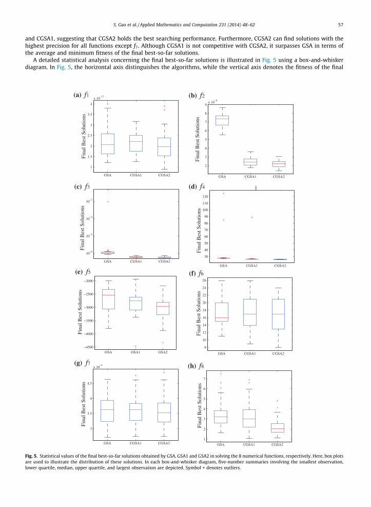
Fig. 6. The average fitness trendlines of the best-so-far solutions found by GSA, CGSA1 and CGSA2 over 30 runs on all tested benchmark functions,respectively. (a) f1 (Sphere), (b) f2 (Schwefel 2.22), (c) f3 (Schwefel 2.21), (d) f4 (Rosenbrock), (e) f5 (Schwefel 2.26), (f) f6 (Rastrigrin), (g) f7 (Ackley), (h) f8

(Griewank).

S. Gao et al. / Applied Mathematics and Computation 231 (2014) 48–62 59

solutions. In particular, for f3, GSA has a probability of generating very bad solutions, indicating that it has trapped in localoptima. Contrarily, both CGSA1 and CGSA2 can always generate relatively good solutions, which demonstrates that the chaossystem definitely enables GSA to have ability of jumping out of local optima. Thus, it can be concluded that by incorporatingchaos system into standard GSA, both CGSA1 and CGSA2 have better searching performance than GSA, and CGSA2 yields thebest performance.

(a) (b)

(c) (d)

(e) (f)

(g) (h)

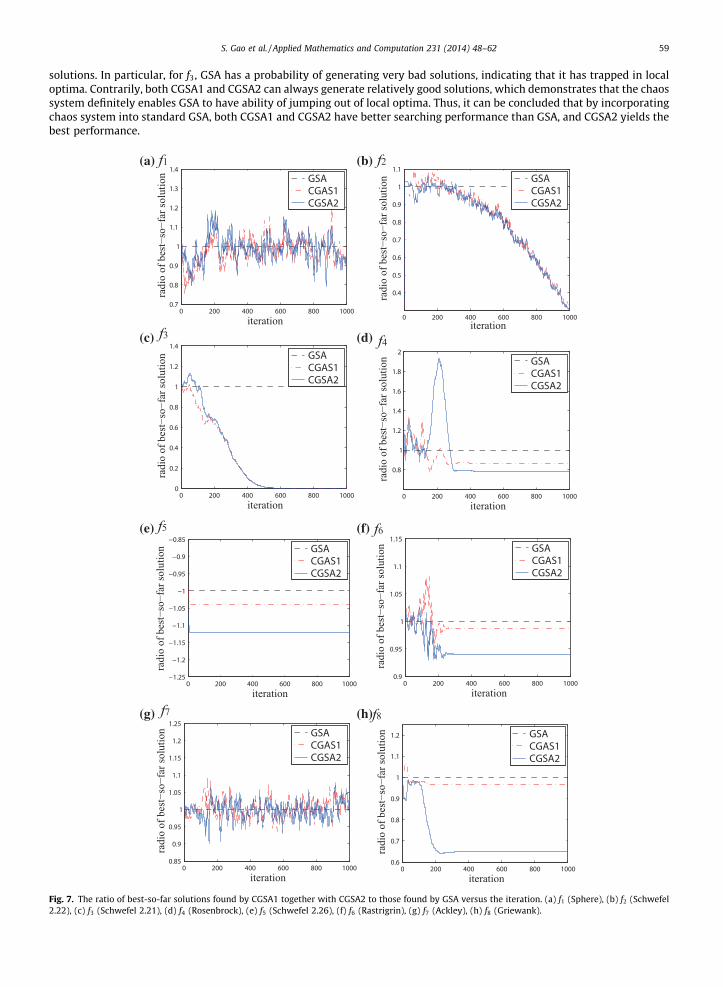
Fig. 7. The ratio of best-so-far solutions found by CGSA1 together with CGSA2 to those found by GSA versus the iteration. (a) f1 (Sphere), (b) f2 (Schwefel2.22), (c) f3 (Schwefel 2.21), (d) f4 (Rosenbrock), (e) f5 (Schwefel 2.26), (f) f6 (Rastrigrin), (g) f7 (Ackley), (h) f8 (Griewank).

60 S. Gao et al. / Applied Mathematics and Computation 231 (2014) 48–62

Besides, in order to find out how the embedded chaos system works, the convergence trendlines produced by these algo-rithms are necessary to be exhibited. Firstly, the average fitness trendlines of the best-so-far solutions generated by GSA,CGSA1 and CGSA2 are illustrated in Fig. 6, where the horizontal axis in linear scales denotes the iteration number of the algo-rithm, while the vertical axis in logarithmic scales represents the average fitness of the best-so-far solutions generated byeach algorithm. Moreover, the convergence graphs of the last 100 iterations are also plotted as subfigures. From this figure,we can find that all three algorithms have a similar convergence process for all tested instances except f3, f5 and f8, thussuggesting that the search in the solution space is mainly driven by gravitational forces during agents rather than the chaoticmechanisms. Even though, it is evident that both CGSA1 and CGSA2 still have abilities to find better solutions in the lattersearch phases, while GSA possibly have already been trapped in local optima.

Alternatively, Fig. 7 depicts the ratio of best-so-far solutions found by CGSA1 together with CGSA2 to those found by GSAversus the iteration, for a clearer illustration. Mathematically, we suppose AFGSA;AFCGSA1 and AFCGSA2 denote the average fit-ness of best-so-far solution found by GSA, CGSA1 and CGSA2, respectively. The ratio can be defined as:

Fig. 8.all 8 fu

Ratio ¼ AFcandidate

AFGSA; candidate 2 fGSA;CGSA1; CGSA2g: ð18Þ

In Fig. 7, the values of the solutions found by GSA are set as the basis, therefore these values form a horizontal line in thefigure. The values above this line denote worse solutions found by the algorithm than those by GSA, while the values belowthis line represent better ones. From Figs. 7(b), (c), (d), (e), (f), and (h), it is clear that both CGSA1 and CGSA2 perform betterthan GSA on tested functions f2—f6 and f8. These figures show that, in the earlier search phases, CGSA1 and CGSA2 generateonly competitive solutions when compared with GSA. The reason is that, during these periods, the algorithms have not con-verged, and meanwhile chaos system always makes the algorithm search in an ergodic space which is a guarantee of prom-ising area while not a better solution temporarily. Nevertheless, with running time goes, there are more and more valuesgenerated by CGSA1 and CGSA2 below the horizontal line of GSA, which indicates that even though GSA approaches to astable solution or can not find better solutions anymore, CGSA1 and CGSA2 still have abilities of finding better solutions, thusleading a better performance than GSA. The above analysis demonstrate that chaos system has definitely helped GSA findbetter solutions, thereafter resulting in better convergence and performance. In addition, the reason of that CGSA1 andCGSA2 have no distinct superiority over GSA for functions f1; f7, is because within 1000 iterations all three algorithms havenot converged and still have very powerful ability to search better solutions (see Fig. 6(a) and (g)). In this case, the improve-ment that chaos system acts on GSA is negligible compared with the performance of GSA itself.

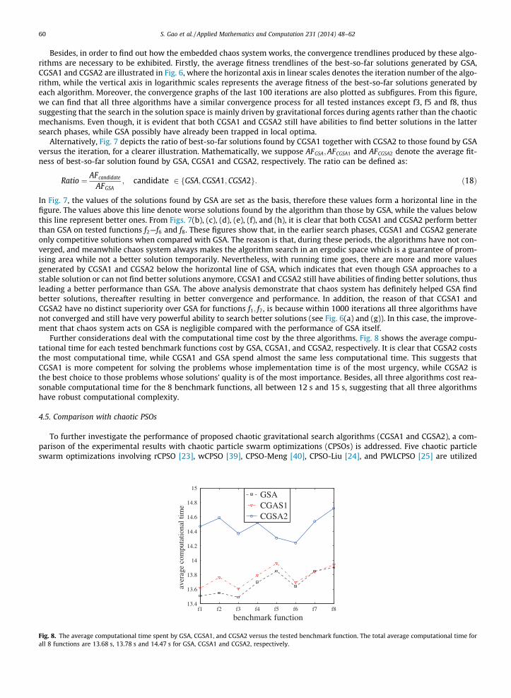
Further considerations deal with the computational time cost by the three algorithms. Fig. 8 shows the average compu-tational time for each tested benchmark functions cost by GSA, CGSA1, and CGSA2, respectively. It is clear that CGSA2 coststhe most computational time, while CGSA1 and GSA spend almost the same less computational time. This suggests thatCGSA1 is more competent for solving the problems whose implementation time is of the most urgency, while CGSA2 isthe best choice to those problems whose solutions’ quality is of the most importance. Besides, all three algorithms cost rea-sonable computational time for the 8 benchmark functions, all between 12 s and 15 s, suggesting that all three algorithmshave robust computational complexity.

4.5. Comparison with chaotic PSOs

To further investigate the performance of proposed chaotic gravitational search algorithms (CGSA1 and CGSA2), a com-parison of the experimental results with chaotic particle swarm optimizations (CPSOs) is addressed. Five chaotic particleswarm optimizations involving rCPSO [23], wCPSO [39], CPSO-Meng [40], CPSO-Liu [24], and PWLCPSO [25] are utilized

f1 f2 f3 f4 f5 f6 f7 f813.4

13.6

13.8

14

14.2

14.4

14.6

14.8

15

benchmark function

ave

rage

com

puta

tiona

l tim

e

GSA CGAS1 CGSA2

The average computational time spent by GSA, CGSA1, and CGSA2 versus the tested benchmark function. The total average computational time fornctions are 13.68 s, 13.78 s and 14.47 s for GSA, CGSA1 and CGSA2, respectively.

Table 4Comparison results based on 4 benchmark functions during CGSA1, CGSA2 and other five typical chaotic particle swarm optimization algorithms (CPSOs).

rCPSO [23] wCPSO [39] CPSO-Meng [40] CPSO-Liu [24] PWLCPSO [25] CGSA1 CGSA2

f1 Precision error 368.32 0.0019 5.25E�77 0.00078 4.05E�79 9.91E�86 1.39E�88Success rate (0.01) 0 0.96 1 0.98 1 1 1Convergence speed inf 3774.7 223.84 582.33 188.80 68.79 72.35

f4 Precision error 49179 328.32 13.003 131.20 12.455 22.17 9.35Success rate (100) 0 0.28 1 0.72 1 1 1Convergence speed inf 3685.4 105.36 958.53 253.44 68.95 72.6

f6 Precision error 158.03 43.01 11.80 56.39 47.28 8.37 7.34Success rate (100) 0.02 1 1 0.96 1 1 1Convergence speed 3357 946.72 47.66 429.54 79.30 68.5 72.6

f7 Precision error 14.57 8.57 0.32 1.30 0.28 4.25E�15 4.0E�15Success rate (0.1) 0 0.46 0.74 0.32 0.78 1 1Convergence speed inf 3297 179.76 2262.30 180.49 69.2 72.7

S. Gao et al. / Applied Mathematics and Computation 231 (2014) 48–62 61

to make the comparison. Both rCPSO and wCPSO use a chaotic map to control the values of the parameters in the velocityupdating process and the value of inertia weight; while CPSO-Meng, CPSO-Liu and PWLCPSO use chaotic search as a localsearch procedure of PSO.

In all compared algorithms, the population size is set to 30, the maximum number of iteration is 5000 in each run, and themaximum iteration number for chaotic search is set to 500. Each algorithm repeats 50 runs. Furthermore, three importantcriteria are employed to evaluate the performance of all algorithms. The convergence precision error indicates the differencebetween the global minimum (Opt.) shown in Table 2 and the actual value of the final best-so-far solution. The success raterepresents the rate of the number of times of successful running to that of total running, indicating the robustness of thealgorithm. The convergence speed is measured by the computational time of evaluation before convergence. This value isasserted to the total computational time if an algorithm has not converged until the maximum iteration number is reached.

Table 4 shows the simulation results of the CPSOs, CGSA1 and CGSA2. The values in the brackets behind the success raterepresent the error threshold to determine a successful run. The symbol inf denotes the algorithm cannot converge withinthe error threshold. From Table 4, it is evident that the robustness of CGSA1 and CGSA2 outperforms CPSOs in all testedbenchmark functions. The success rate of CGSA1 and CGSA2 always maintains 100%. In particular, CGSA2 can obtain the bestprecision error for all functions within a reasonable computational time. From another point of view, CPSO-Meng, CPSO-Liuand PWLCPSO perform better than rCPSO and wCPSO, meanwhile CGSA2 outperforms CGSA1, suggesting that the embeddedmethod of using chaos system as a local search approach is generally better than that as a chaotic sequence generator tosubstitute random sequences.

5. Conclusions

To our knowledge, this was the first report of hybridizing gravitational search algorithm (GSA) and chaos to propose aneffective and efficient optimization algorithm for numerical functions. Two kinds of hybridization methodologies were pro-posed. One used chaos to generate chaotic sequences to substitute random sequences of the parameters in GSA, and theother employed chaos to perform a local search approach. Experimental results based on a number of benchmark functionsshowed that both emerged chaotic gravitational search algorithms (CGSAs) had better performance than GSA. Comparisonresults with other five typical chaotic particle swarm optimization algorithms verified the superiorities of proposed CGSAs.Furthermore, the embedded method of using chaos as a local search could improve the performance of GSA much better thanthe other embedded method, thus remaining an evidence of the choice of embedded methods when incorporating chaos intoother meta-heuristics. In the future, we plan to combine both embedded methods with GSA synchronously to validate theemerged new hybrid algorithm.

Acknowledgements

This work is partially supported by the National Natural Science Foundation of China under Grants 61203325. We wouldlike to give thanks to the anonymous reviewer for the valuable suggestions to further improve the quality of the paper.

References

[1] K. Aardal, S. Hoesel, J. Lenstra, L. Stougie, A decade of combinatorial optimization, Tech. Rep. UU-CS-1997-12, Department of Information andComputing Sciences, Utrecht University, 1997.

[2] P. Festa, M.G.C. Resende, Hybrid grasp heuristics, Tech. Rep. NJ 07932, AT&T Labs Research, Florham Park, USA, 2008.[3] E.H.L. Aarts, J.H.M. Korst, P.J.M. van Laarhoven, Simulated Annealing, John Wiley & Sons, Chichester, UK, 1997. 91–120.[4] M. Dorigo, T. St}utzle, Ant Colony Optimization, MIT press, 2004.[5] K. Passino, Biomimicry of bacterial foraging for distributed optimization and control, IEEE Control Syst. Mag. 22 (2002) 52–67.

62 S. Gao et al. / Applied Mathematics and Computation 231 (2014) 48–62

[6] S.J. Russell, P. Norvig, Artificial Intelligence: A Modern Approach, Prentice Hall, Upper Saddle River, New Jersey, 2003.[7] J. Kennedy, R. Eberhart, Particle swarm optimization, in: Proceedings of IEEE International Conference on Neural Networks, 1995, pp. 1942–1948.[8] D.H. Wolpert, W.G. Macready, No free lunch theorems for optimization, IEEE Trans. Evol. Comput. 1 (1997) 67–82.[9] E. Rashedi, H. Nezamabadi-pour, S. Saryazdi, GSA: a gravitational search algorithm, Inf. Sci. 179 (13) (2009) 2232–2248.

[10] E. Rashedi, H. Nezamabadi-pour, S. Saryazdi, BGSA: binary gravitational search algorithm, Nat. Comput. 3 (9) (2010) 727–745.[11] B. Zibanezhad, K. Zamanifar, N. Nematbakhsh, F. Mardukhi, An approach for web services composition based on qos and gravitational search algorithm,

in: Proceedings of the 6th International Conference on Innovations in Information Technology, AI-Ain, United Arab Emirates, 2009, pp. 121–125.[12] S.R. Balachandar, K. Kannan, A meta-heuristic algorithm for vertex covering problem based on gravity, Int. J. Math. Stat. Sci. 1 (3) (2009) 130–136.[13] C. Lopez-Molina, H. Bustince, J. Fernandez, P. Couto, B.D. Baets, A Gravitational approach to edge detection based on triangular norms, Pattern Recognit.

43 (2010) 3730–3741.[14] C.S. Li, J.Z. Zhou, Parameters identification of hydraulic turbine governing system using improved gravitational search algorithm, Energy Convers.

Manage. 52 (1) (2011) 374–381.[15] C. Blum, Ant colony optimization: introduction and recent trends, Phys. Life Rev. 2 (2005) 353–373.[16] E. Ott, C. Grebogi, J.A. Yorke, Controlling chaos, Phys. Rev. Lett. 64 (1990) 1196–1199.[17] C. Zhou, T. Chen, Chaotic annealing for optimisation, Phys. Rev. E 55 (3) (1997) 2580–2587.[18] B. Li, W. Jiang, Optimizing complex functions by chaos search, Cybern. Syst. 29 (4) (1998) 409–419.[19] M. Ji, H. Tang, Application of chaos in simulated annealing, Chaos Solitons Fract. 21 (2004) 933–941.[20] Y. Li, Q. Wen, L. Li, H. Peng, Hybrid chaotic ant swarm optimization, Chaos Solitons Fract. 42 (2009) 880–889.[21] B. Alatas, Chaotic harmony search algorithms, Appl. Math. Comput. 216 (2010) 2687–2699.[22] B. Alatas, Chaotic bee colony algorithms for global numerical optimization, Expert Syst. Appl. 37 (2010) 5682–5687.[23] C. Jiang, E. Bompard, A self-adaptive chaotic particle swarm algorithm for short term hydroelectric system scheduling in deregulated environment,

Energy Convers. Manage. 46 (2005) 2689–2696.[24] B. Liu, L. Wang, Y.H. Jin, F. Tang, D.X. Huang, Improved particle swarm optimization combined with chaos, Chaos Solitons Fract. 25 (2005) 1261–1271.[25] T. Xiang, X. Liao, K. Wong, An improved particle swarm optimization algorithm combined with piecewise linear chaotic map, Appl. Math. Comput. 190

(2007) 1637–1645.[26] B. Alatas, E. Akin, A.B. Ozer, Chaos embedded particle swarm optimization algorithms, Chaos Solitons Fract. 40 (2009) 1715–1734.[27] C. Lng, S.Q. Li, Chaotic spreading sequences with multiple access performance better than random sequences, IEEE Trans. Circuit Syst. I, Fundam.

Theory Appl. 47 (3) (2000) 394–397.[28] R.M. May, Simple mathematical models with very complicated dynamics, Nature 261 (1976) 459.[29] M.J. Ji, H.W. Tang, Application of chaos in simulated annealing, Chaos Solitons Fract. 21 (2004) 933–941.[30] I.C. Trelea, The particle swarm optimization algorithm: convergence analysis and parameter selection, Inf. Process. Lett. 85 (6) (2003) 317–325.[31] Y. Shi, R.C. Eberhart, Parameter selection in particle swarm optimization, Lecture Notes Comput. Sci., Evol. Program. VII 1447 (1998) 591–600.[32] Y.L. Zheng, L.H. Ma, L.Y. Zhang, J.X. Qian, On the convergence analysis and parameter selection in particle swarm optimization, in: Proc. of the 2003

IEEE International Conference on Machine Learning and Cybernetics, Piscataway, NJ, 2003, pp. 1802–1807.[33] Y.L. Zheng, L.H. Ma, L.Y. Zhang, J.X. Qian, Empirical study of particle swarm optimizer with an increasing inertia weight, in: Proc. of the 2003 IEEE

Congress on Evolutionary Computation, Piscataway, NJ, 2003, pp. 221–226.[34] B. Jiao, Z.G. Lian, X.S. Gu, A dynamic inertia weight particle swarm optimization algorithm, Chaos Solitons Fract. 37 (3) (2008) 698–705.[35] Y. Shi, R.C. Eberhart, Fuzzy adaptive particle swarm optimization, in: Proc. of the 2001 IEEE Congress on Evolutionary Computation, Piscataway, NJ,

2001, pp. 101–106.[36] L. Zhang, H. Yu, S. Hu, A new approach to improve particle swarm optimization, in: Lecture Notes in Computer Science, GECCO, 2003, pp. 134–139.[37] R.C. Eberhart, Y. Shi, Tracking and optimizing dynamic systems with particle swarms, in: Proc. of the 2001 IEEE Congress on Evolutionary Computation,

Piscataway, NJ, 2001, pp. 94–100.[38] J.B. Park, Y.W. Jeong, H.H. Kim, J.R. Shin, An improved particle swarm optimization for economic dispatch with valve-point effect, Int. J. Innov. Energy

Syst. Power 1 (1) (2006) 1–7.[39] C. Jiang, E. Bompard, A hybrid method of chaotic particle swarm optimization and linear interior for reactive power optimization, Math. Comput. Simul.

68 (2005) 57–65.[40] H. Meng, P. Zheng, R. Wu, X. Hao, Z. Xie, A hybrid particle swarm algorithm with embedded chaotic search, in: Proc. of IEEE Conference on Cybernetics

and Intelligent Systems, Singapore, 2004, pp. 367–371.