02/09/2006 CS267 Lecture 8 1 CS 267 Dense Linear Algebra: Parallel Matrix Multiplication James Demmel www.cs.berkeley.edu/~demmel/ cs267_Spr06

Welcome message from author
This document is posted to help you gain knowledge. Please leave a comment to let me know what you think about it! Share it to your friends and learn new things together.
Transcript

02/09/2006 CS267 Lecture 8 1
CS 267Dense Linear Algebra:
Parallel Matrix Multiplication
James Demmel
www.cs.berkeley.edu/~demmel/cs267_Spr06

02/09/2006 CS267 Lecture 8 2
Outline
• Recall BLAS = Basic Linear Algebra Subroutines• Matrix-vector multiplication in parallel• Matrix-matrix multiplication in parallel

02/09/2006 CS267 Lecture 8 3
Review of the BLAS
BLAS level Ex. # mem refs # flops q
1 “Axpy”, Dot prod
3n 2n1 2/3
2 Matrix-vector mult
n2 2n2 2
3 Matrix-matrix mult
4n2 2n3 n/2
• Building blocks for all linear algebra• Parallel versions call serial versions on each processor
• So they must be fast!• Recall q = # flops / # mem refs
• The larger is q, the faster the algorithm can go in the presence of memory hierarchy
• “axpy”: y = *x + y, where scalar, x and y vectors
02/09/2006 CS267 Lecture 8 4
Different Parallel Data Layouts for Matrices
0123012301230123
0 1 2 3 0 1 2 3
1) 1D Column Blocked Layout 2) 1D Column Cyclic Layout
3) 1D Column Block Cyclic Layout
4) Row versions of the previous layouts
Generalizes others
0 1 0 1 0 1 0 12 3 2 3 2 3 2 30 1 0 1 0 1 0 12 3 2 3 2 3 2 30 1 0 1 0 1 0 12 3 2 3 2 3 2 30 1 0 1 0 1 0 12 3 2 3 2 3 2 3 6) 2D Row and Column
Block Cyclic Layout
0 1 2 3
0 1
2 3
5) 2D Row and Column Blocked Layout
b
02/09/2006 CS267 Lecture 8 5
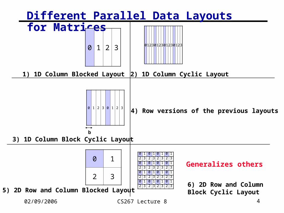
Parallel Matrix-Vector Product• Compute y = y + A*x, where A is a dense matrix• Layout:
• 1D row blocked
• A(i) refers to the n by n/p block row that processor i owns,
• x(i) and y(i) similarly refer to segments of x,y owned by i
• Algorithm:• Foreach processor i• Broadcast x(i)• Compute y(i) = A(i)*x
• Algorithm uses the formulay(i) = y(i) + A(i)*x = y(i) + j A(i,j)*x(j)
x
y
P0
P1
P2
P3
P0 P1 P2 P3
02/09/2006 CS267 Lecture 8 6
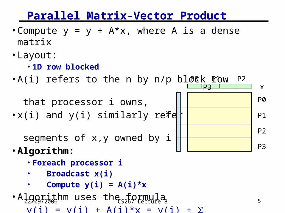
Matrix-Vector Product y = y + A*x
• A column layout of the matrix eliminates the broadcast of x• But adds a reduction to update the destination y
• A 2D blocked layout uses a broadcast and reduction, both on a subset of processors
• sqrt(p) for square processor grid
P0 P1 P2 P3
P0 P1 P2 P3
P4 P5 P6 P7
P8 P9 P10 P11
P12 P13 P14 P15

02/09/2006 CS267 Lecture 8 7
Parallel Matrix Multiply
• Computing C=C+A*B• Using basic algorithm: 2*n3 Flops• Variables are:
• Data layout• Topology of machine • Scheduling communication
• Use of performance models for algorithm design• Message Time = “latency” + #words * time-per-word
= + n*• Efficiency (in any model):
• serial time / (p * parallel time)• perfect (linear) speedup efficiency = 1
02/09/2006 CS267 Lecture 8 8
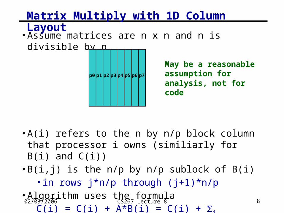
Matrix Multiply with 1D Column Layout
• Assume matrices are n x n and n is divisible by p
• A(i) refers to the n by n/p block column that processor i owns (similiarly for B(i) and C(i))
• B(i,j) is the n/p by n/p sublock of B(i) • in rows j*n/p through (j+1)*n/p
• Algorithm uses the formulaC(i) = C(i) + A*B(i) = C(i) + j A(j)*B(j,i)
p0 p1 p2 p3 p5 p4 p6 p7
May be a reasonable assumption for analysis, not for code

02/09/2006 CS267 Lecture 8 9
Matrix Multiply: 1D Layout on Bus or Ring
• Algorithm uses the formulaC(i) = C(i) + A*B(i) = C(i) + j A(j)*B(j,i)
• First consider a bus-connected machine without broadcast: only one pair of processors can communicate at a time (ethernet)
• Second consider a machine with processors on a ring: all processors may communicate with nearest neighbors simultaneously

02/09/2006 CS267 Lecture 8 10
MatMul: 1D layout on Bus without Broadcast
Naïve algorithm: C(myproc) = C(myproc) + A(myproc)*B(myproc,myproc)
for i = 0 to p-1 for j = 0 to p-1 except i if (myproc == i) send A(i) to processor j if (myproc == j) receive A(i) from processor i C(myproc) = C(myproc) + A(i)*B(i,myproc) barrier
Cost of inner loop: computation: 2*n*(n/p)2 = 2*n3/p2 communication: + *n2 /p

02/09/2006 CS267 Lecture 8 11
Naïve MatMul (continued)
Cost of inner loop: computation: 2*n*(n/p)2 = 2*n3/p2 communication: + *n2 /p … approximately
Only 1 pair of processors (i and j) are active on any iteration, and of those, only i is doing computation => the algorithm is almost entirely serial
Running time: = (p*(p-1) + 1)*computation + p*(p-1)*communication ~= 2*n3 + p2* + p*n2*
This is worse than the serial time and grows with p.Why might you still want to do this?

02/09/2006 CS267 Lecture 8 12
Matmul for 1D layout on a Processor Ring
• Pairs of processors can communicate simultaneously
Copy A(myproc) into Tmp
C(myproc) = C(myproc) + Tmp*B(myproc , myproc)
for j = 1 to p-1
Send Tmp to processor myproc+1 mod p
Receive Tmp from processor myproc-1 mod p
C(myproc) = C(myproc) + Tmp*B( myproc-j mod p , myproc)
• Same idea as for gravity in simple sharks and fish algorithm
• May want double buffering in practice for overlap
• Ignoring deadlock details in code• Time of inner loop = 2*( + *n2/p) + 2*n*(n/p)2

02/09/2006 CS267 Lecture 8 13
Matmul for 1D layout on a Processor Ring
• Time of inner loop = 2*( + *n2/p) + 2*n*(n/p)2
• Total Time = 2*n* (n/p)2 + (p-1) * Time of inner loop• ~ 2*n3/p + 2*p* + 2**n2
• Optimal for 1D layout on Ring or Bus, even with with Broadcast:
• Perfect speedup for arithmetic• A(myproc) must move to each other processor, costs at
least (p-1)*cost of sending n*(n/p) words
• Parallel Efficiency = 2*n3 / (p * Total Time) = 1/(1 + * p2/(2*n3) + * p/(2*n) ) = 1/ (1 + O(p/n))• Grows to 1 as n/p increases (or and shrink)

02/09/2006 CS267 Lecture 8 14
MatMul with 2D Layout
• Consider processors in 2D grid (physical or logical)• Processors can communicate with 4 nearest neighbors
• Broadcast along rows and columns
• Assume p processors form square s x s grid
p(0,0) p(0,1) p(0,2)
p(1,0) p(1,1) p(1,2)
p(2,0) p(2,1) p(2,2)
p(0,0) p(0,1) p(0,2)
p(1,0) p(1,1) p(1,2)
p(2,0) p(2,1) p(2,2)
p(0,0) p(0,1) p(0,2)
p(1,0) p(1,1) p(1,2)
p(2,0) p(2,1) p(2,2)
= *

02/09/2006 CS267 Lecture 8 15
Cannon’s Algorithm
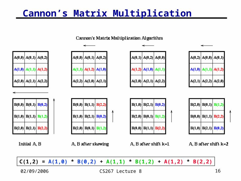
… C(i,j) = C(i,j) + A(i,k)*B(k,j)… assume s = sqrt(p) is an integer forall i=0 to s-1 … “skew” A left-circular-shift row i of A by i … so that A(i,j) overwritten by A(i,(j+i)mod s) forall i=0 to s-1 … “skew” B up-circular-shift column i of B by i … so that B(i,j) overwritten by B((i+j)mod s), j) for k=0 to s-1 … sequential forall i=0 to s-1 and j=0 to s-1 … all processors in parallel C(i,j) = C(i,j) + A(i,j)*B(i,j) left-circular-shift each row of A by 1 up-circular-shift each column of B by 1
k
02/09/2006 CS267 Lecture 8 16
C(1,2) = A(1,0) * B(0,2) + A(1,1) * B(1,2) + A(1,2) * B(2,2)
Cannon’s Matrix Multiplication

02/09/2006 CS267 Lecture 8 17
Initial Step to Skew Matrices in Cannon
• Initial blocked input
• After skewing before initial block multiplies
A(0,1) A(0,2)
A(1,0)
A(2,0)
A(1,1) A(1,2)
A(2,1)A(2,2)
A(0,0)
B(0,1) B(0,2)
B(1,0)
B(2,0)
B(1,1) B(1,2)
B(2,1) B(2,2)
B(0,0)A(0,1) A(0,2)
A(1,0)
A(2,0)
A(1,1) A(1,2)
A(2,1) A(2,2)
A(0,0)
B(0,1)
B(0,2)B(1,0)
B(2,0)
B(1,1)
B(1,2)
B(2,1)
B(2,2)B(0,0)
02/09/2006 CS267 Lecture 8 18
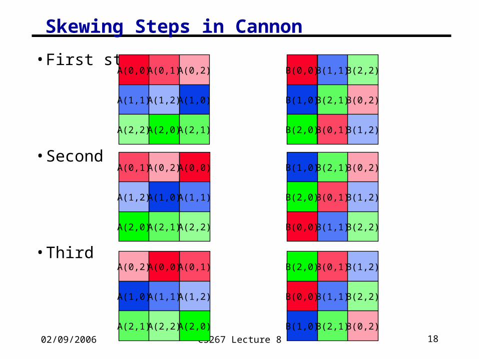
Skewing Steps in Cannon
• First step
• Second
• Third
A(0,1) A(0,2)
A(1,0)
A(2,0)
A(1,1) A(1,2)
A(2,1)A(2,2)
A(0,0)
B(0,1)
B(0,2)B(1,0)
B(2,0)
B(1,1)
B(1,2)
B(2,1)
B(2,2)B(0,0)
A(0,1) A(0,2)
A(1,0)
A(2,0)
A(1,2)
A(2,1)
B(0,1)
B(0,2)B(1,0)
B(2,0)
B(1,1)
B(1,2)
B(2,1)
B(2,2)B(0,0)
A(0,1)A(0,2)
A(1,0)
A(2,0)
A(1,1) A(1,2)
A(2,1) A(2,2)
A(0,0) B(0,1)
B(0,2)B(1,0)
B(2,0)
B(1,1)
B(1,2)
B(2,1)
B(2,2)B(0,0)
A(1,1)
A(2,2)
A(0,0)

02/09/2006 CS267 Lecture 8 19
Cost of Cannon’s Algorithm forall i=0 to s-1 … recall s = sqrt(p) left-circular-shift row i of A by i … cost = s*( + *n2/p) forall i=0 to s-1 up-circular-shift column i of B by i … cost = s*( + *n2/p) for k=0 to s-1 forall i=0 to s-1 and j=0 to s-1
C(i,j) = C(i,j) + A(i,j)*B(i,j) … cost = 2*(n/s)3 = 2*n3/p3/2
left-circular-shift each row of A by 1 … cost = + *n2/p up-circular-shift each column of B by 1 … cost = + *n2/p
° Total Time = 2*n3/p + 4* s* + 4**n2/s ° Parallel Efficiency = 2*n3 / (p * Total Time)
= 1/( 1 + * 2*(s/n)3 + * 2*(s/n) ) = 1/(1 + O(sqrt(p)/n)) ° Grows to 1 as n/s = n/sqrt(p) = sqrt(data per processor) grows° Better than 1D layout, which had Efficiency = 1/(1 + O(p/n))
02/09/2006 CS267 Lecture 8 20
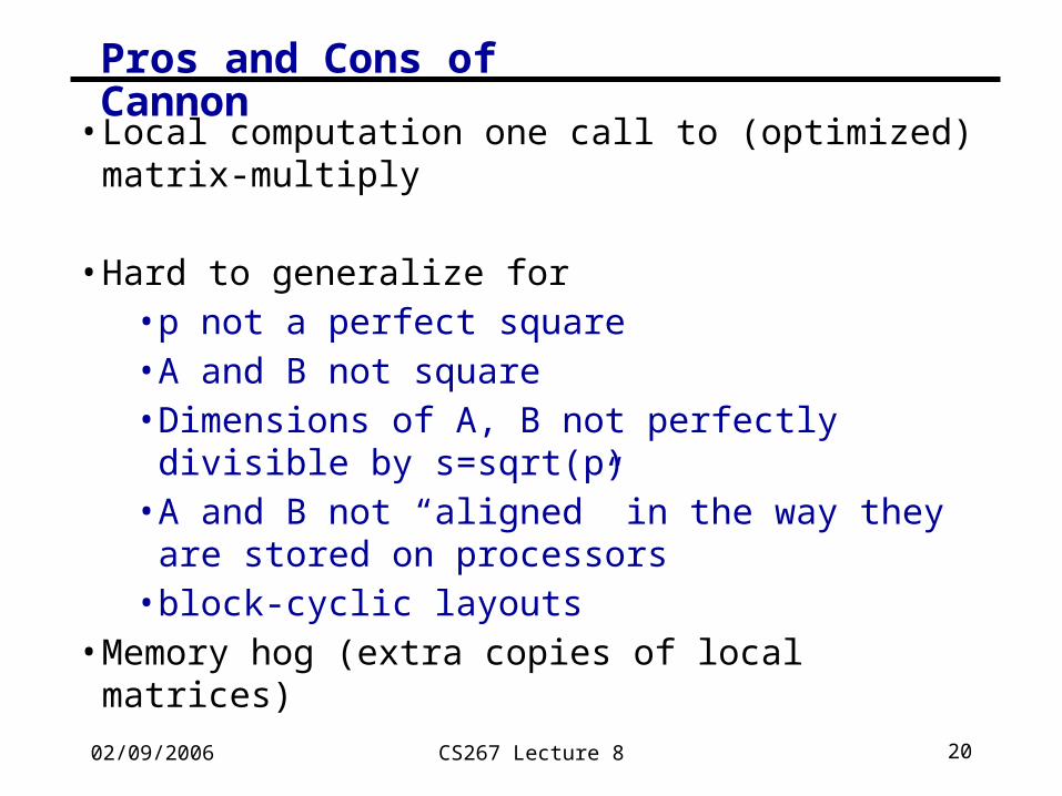
Pros and Cons of Cannon
• Local computation one call to (optimized) matrix-multiply
• Hard to generalize for• p not a perfect square• A and B not square• Dimensions of A, B not perfectly divisible by
s=sqrt(p)• A and B not “aligned” in the way they are stored on
processors• block-cyclic layouts
• Memory hog (extra copies of local matrices)
02/09/2006 CS267 Lecture 8 21
SUMMA Algorithm
• SUMMA = Scalable Universal Matrix Multiply • Slightly less efficient, but simpler and easier to
generalize• Presentation from van de Geijn and Watts
• www.netlib.org/lapack/lawns/lawn96.ps• Similar ideas appeared many times
• Used in practice in PBLAS = Parallel BLAS• www.netlib.org/lapack/lawns/lawn100.ps
02/09/2006 CS267 Lecture 8 22
SUMMA
* =i
j
A(i,k)
k
k
B(k,j)
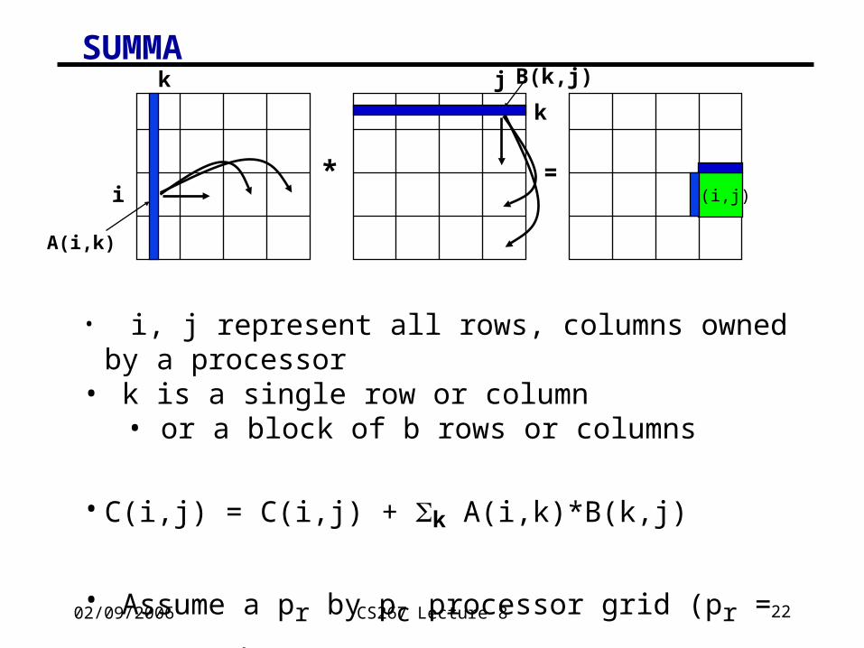
• i, j represent all rows, columns owned by a processor• k is a single row or column
• or a block of b rows or columns
• C(i,j) = C(i,j) + k A(i,k)*B(k,j)
• Assume a pr by pc processor grid (pr = pc = 4 above) • Need not be square
C(i,j)

02/09/2006 CS267 Lecture 8 23
SUMMA
For k=0 to n-1 … or n/b-1 where b is the block size
… = # cols in A(i,k) and # rows in B(k,j)
for all i = 1 to pr … in parallel
owner of A(i,k) broadcasts it to whole processor row
for all j = 1 to pc … in parallel
owner of B(k,j) broadcasts it to whole processor column
Receive A(i,k) into Acol
Receive B(k,j) into Brow
C_myproc = C_myproc + Acol * Brow
* =i
j
A(i,k)
k
k
B(k,j)
C(i,j)
02/09/2006 CS267 Lecture 8 24
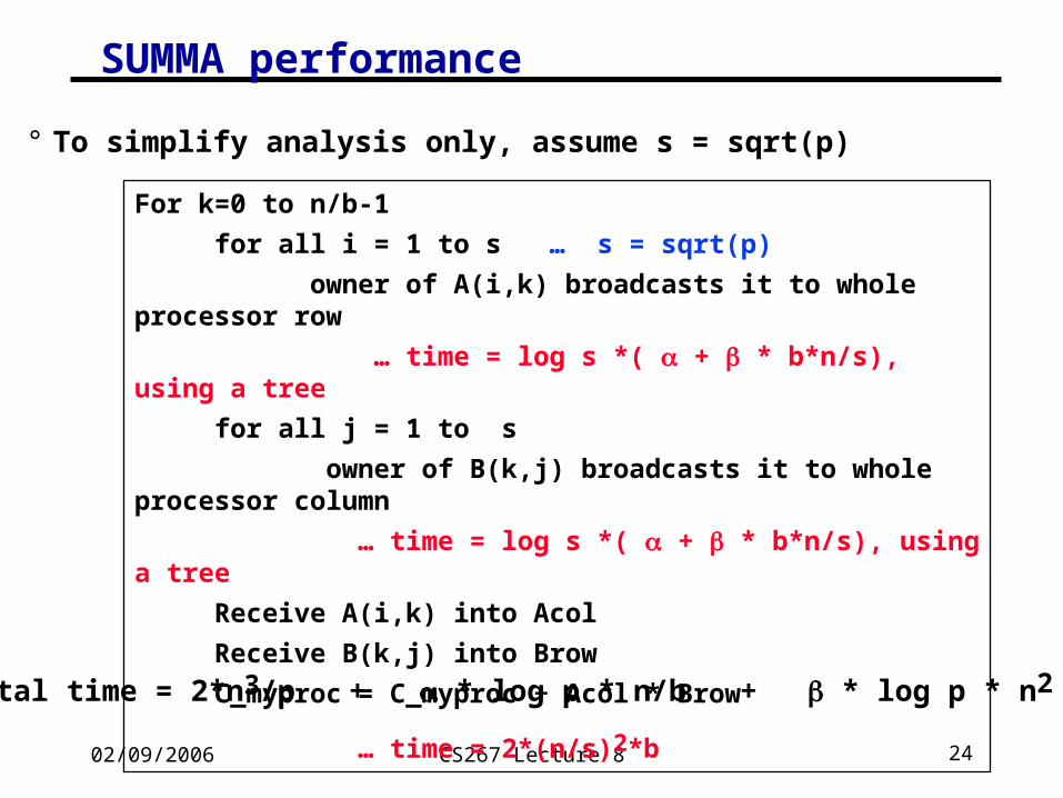
SUMMA performance
For k=0 to n/b-1
for all i = 1 to s … s = sqrt(p)
owner of A(i,k) broadcasts it to whole processor row
… time = log s *( + * b*n/s), using a tree
for all j = 1 to s
owner of B(k,j) broadcasts it to whole processor column
… time = log s *( + * b*n/s), using a tree
Receive A(i,k) into Acol
Receive B(k,j) into Brow
C_myproc = C_myproc + Acol * Brow
… time = 2*(n/s)2*b
° Total time = 2*n3/p + * log p * n/b + * log p * n2 /s
° To simplify analysis only, assume s = sqrt(p)

02/09/2006 CS267 Lecture 8 25
SUMMA performance
• Total time = 2*n3/p + * log p * n/b + * log p * n2 /s
• Parallel Efficiency =
1/(1 + * log p * p / (2*b*n2) + * log p * s/(2*n) )
• ~Same term as Cannon, except for log p factor
log p grows slowly so this is ok
• Latency () term can be larger, depending on b
When b=1, get * log p * n
As b grows to n/s, term shrinks to
* log p * s (log p times Cannon)
• Temporary storage grows like 2*b*n/s
• Can change b to tradeoff latency cost with memory
02/09/2006 CS267 Lecture 8 26
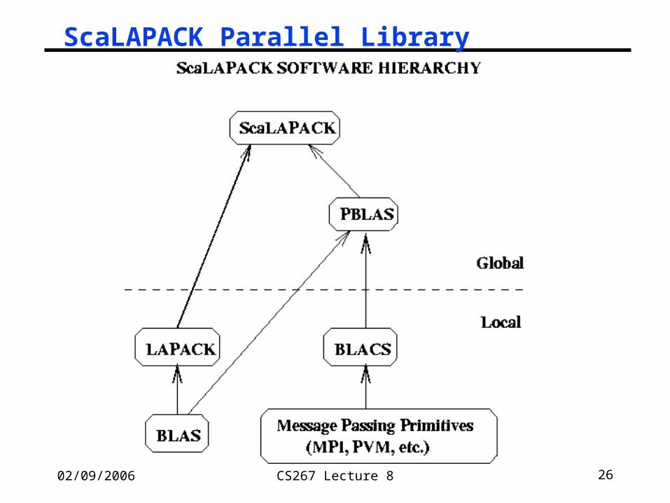
ScaLAPACK Parallel Library

02/09/2006 CS267 Lecture 8 27
PDGEMM = PBLAS routine for matrix multiply
Observations: For fixed N, as P increases Mflops increases, but less than 100% efficiency For fixed P, as N increases, Mflops (efficiency) rises
DGEMM = BLAS routine for matrix multiply
Maximum speed for PDGEMM = # Procs * speed of DGEMM
Observations (same as above): Efficiency always at least 48% For fixed N, as P increases, efficiency drops For fixed P, as N increases, efficiency increases
02/09/2006 CS267 Lecture 8 28
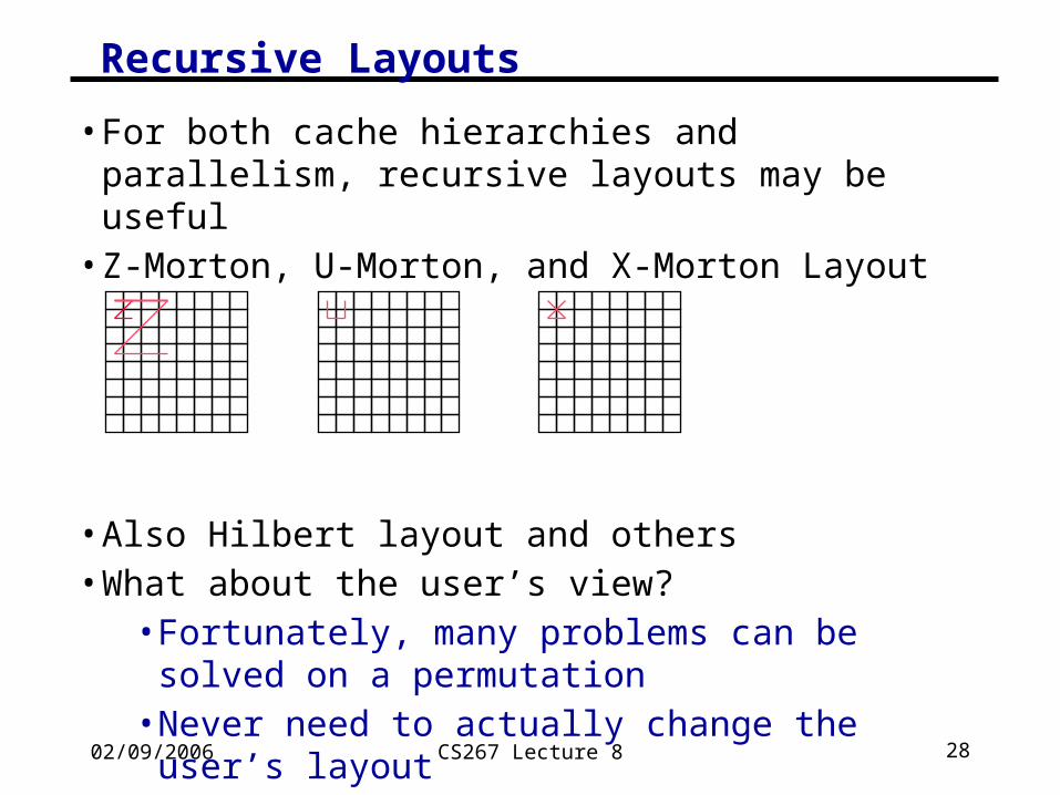
Recursive Layouts
• For both cache hierarchies and parallelism, recursive layouts may be useful
• Z-Morton, U-Morton, and X-Morton Layout
• Also Hilbert layout and others• What about the user’s view?
• Fortunately, many problems can be solved on a permutation
• Never need to actually change the user’s layout

02/09/2006 CS267 Lecture 8 29
Summary of Parallel Matrix Multiplication• 1D Layout
• Bus without broadcast - slower than serial• Nearest neighbor communication on a ring (or bus with
broadcast): Efficiency = 1/(1 + O(p/n))• 2D Layout
• Cannon• Efficiency = 1/(1+O(sqrt(p) /n+* sqrt(p) /n))• Hard to generalize for general p, n, block cyclic, alignment
• SUMMA• Efficiency = 1/(1 + O(log p * p / (b*n2) + log p * sqrt(p) /n))• Very General• b small => less memory, lower efficiency• b large => more memory, high efficiency
• Recursive layouts• Current area of research
02/09/2006 CS267 Lecture 8 30
Extra Slides

02/09/2006 CS267 Lecture 8 31
Gaussian Elimination
0x
x
xx
.
.
.
Standard Waysubtract a multiple of a row
0
x
00
. . .
0
LINPACKapply sequence to a column
x
nb
then apply nb to rest of matrix
a3=a3-a1*a2
a3
a2
a1
L
a2 =L-1
a2
0
x
00
. . .
0
nb LAPACKapply sequence to nb
Slide source: Dongarra

02/09/2006 CS267 Lecture 8 32
LU Algorithm: 1: Split matrix into two rectangles (m x n/2) if only 1 column, scale by reciprocal of pivot & return
2: Apply LU Algorithm to the left part
3: Apply transformations to right part (triangular solve A12 = L-1A12 and matrix multiplication A22=A22 -A21*A12 )
4: Apply LU Algorithm to right part
Gaussian Elimination via a Recursive Algorithm
L A12
A21 A22
F. Gustavson and S. Toledo
Most of the work in the matrix multiply Matrices of size n/2, n/4, n/8, …
Slide source: Dongarra
02/09/2006 CS267 Lecture 8 33
Recursive Factorizations
• Just as accurate as conventional method• Same number of operations• Automatic variable blocking
• Level 1 and 3 BLAS only !• Extreme clarity and simplicity of expression• Highly efficient• The recursive formulation is just a rearrangement of the point-wise
LINPACK algorithm• The standard error analysis applies (assuming the matrix
operations are computed the “conventional” way).
Slide source: Dongarra

02/09/2006 CS267 Lecture 8 34
DGEMM ATLAS & DGETRF Recursive
AMD Athlon 1GHz (~$1100 system)
0
100
200
300
400
500 1000 1500 2000 2500 3000
Order
MFl
op/s
Pentium III 550 MHz Dual Processor LU Factorization
0
200
400
600
800
500 1000 1500 2000 2500 3000 3500 4000 4500 5000
Order
Mflo
p/s
LAPACK
Recursive LU
Recursive LU
LAPACK
Dual-processor
Uniprocessor
Slide source: Dongarra
02/09/2006 CS267 Lecture 8 35
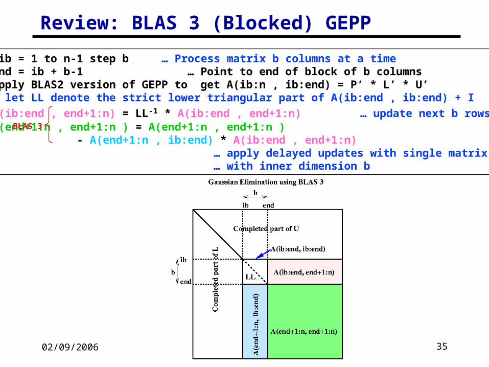
Review: BLAS 3 (Blocked) GEPP
for ib = 1 to n-1 step b … Process matrix b columns at a time end = ib + b-1 … Point to end of block of b columns apply BLAS2 version of GEPP to get A(ib:n , ib:end) = P’ * L’ * U’ … let LL denote the strict lower triangular part of A(ib:end , ib:end) + I
A(ib:end , end+1:n) = LL-1 * A(ib:end , end+1:n) … update next b rows of U A(end+1:n , end+1:n ) = A(end+1:n , end+1:n ) - A(end+1:n , ib:end) * A(ib:end , end+1:n) … apply delayed updates with single matrix-multiply … with inner dimension b
BLAS 3

02/09/2006 CS267 Lecture 8 36
Review: Row and Column Block Cyclic Layout
processors and matrix blocksare distributed in a 2d array
pcol-fold parallelismin any column, and calls to the BLAS2 and BLAS3 on matrices of size brow-by-bcol
serial bottleneck is eased
need not be symmetric in rows andcolumns

02/09/2006 CS267 Lecture 8 37
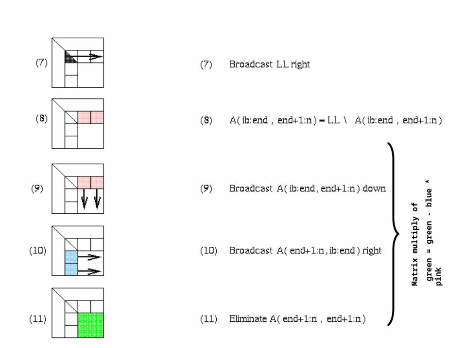
Distributed GE with a 2D Block Cyclic Layout
block size b in the algorithm and the block sizes brow and bcol in the layout satisfy b=brow=bcol.
shaded regions indicate busy processors or communication performed.
unnecessary to have a barrier between each step of the algorithm, e.g.. step 9, 10, and 11 can be pipelined

02/09/2006 CS267 Lecture 8 38
Distributed GE with a 2D Block Cyclic Layout
02/09/2006 CS267 Lecture 8 39
Ma
trix
mu
ltip
ly o
f
gre
en
= g
ree
n -
blu
e *
pin
k
02/09/2006 CS267 Lecture 8 40
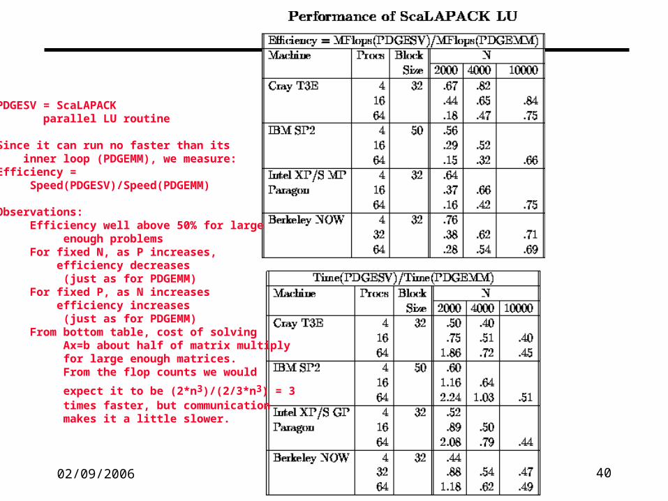
PDGESV = ScaLAPACK parallel LU routine
Since it can run no faster than its inner loop (PDGEMM), we measure:Efficiency = Speed(PDGESV)/Speed(PDGEMM)
Observations: Efficiency well above 50% for large enough problems For fixed N, as P increases, efficiency decreases (just as for PDGEMM) For fixed P, as N increases efficiency increases (just as for PDGEMM) From bottom table, cost of solving Ax=b about half of matrix multiply for large enough matrices. From the flop counts we would
expect it to be (2*n3)/(2/3*n3) = 3 times faster, but communication makes it a little slower.

02/09/2006 CS267 Lecture 8 41

02/09/2006 CS267 Lecture 8 42
Scales well, nearly full machine speed

02/09/2006 CS267 Lecture 8 43
Old version,pre 1998 Gordon Bell Prize
Still have ideas to accelerateProject Available!
Old Algorithm, plan to abandon

02/09/2006 CS267 Lecture 8 44
Have good ideas to speedupProject available!
Hardest of all to parallelizeHave alternative, and would like to compareProject available!
02/09/2006 CS267 Lecture 8 45
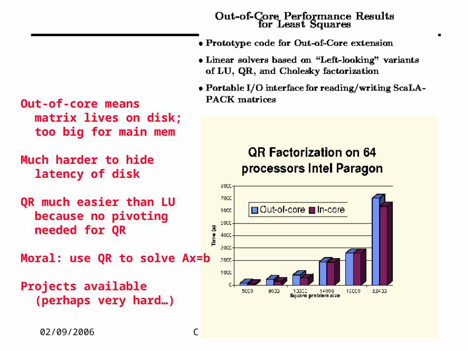
Out-of-core means matrix lives on disk; too big for main mem
Much harder to hide latency of disk
QR much easier than LU because no pivoting needed for QR
Moral: use QR to solve Ax=b
Projects available (perhaps very hard…)

02/09/2006 CS267 Lecture 8 46
A small software project ...

02/09/2006 CS267 Lecture 8 47
Work-Depth Model of Parallelism
• The work depth model:• The simplest model is used• For algorithm design, independent of a machine
• The work, W, is the total number of operations• The depth, D, is the longest chain of dependencies• The parallelism, P, is defined as W/D
• Specific examples include:• circuit model, each input defines a graph with ops at
nodes• vector model, each step is an operation on a vector of
elements• language model, where set of operations defined by
language

02/09/2006 CS267 Lecture 8 48
Latency Bandwidth Model
• Network of fixed number P of processors• fully connected• each with local memory
• Latency ()• accounts for varying performance with number of
messages• gap (g) in logP model may be more accurate cost if
messages are pipelined• Inverse bandwidth ()
• accounts for performance varying with volume of data• Efficiency (in any model):
• serial time / (p * parallel time)• perfect (linear) speedup efficiency = 1
Related Documents