Biologically Inspired Vision and Control for an Autonomous Flying Vehicle Matthew A. Garratt A thesis submitted for the degree of Doctor of Philosophy of the The Australian National University October, 2007

02 Whole
Sep 23, 2014
Welcome message from author
This document is posted to help you gain knowledge. Please leave a comment to let me know what you think about it! Share it to your friends and learn new things together.
Transcript
Biologically Inspired Vision and Control
for an Autonomous Flying Vehicle
Matthew A. Garratt
A thesis submitted for the degree of
Doctor of Philosophy of the
The Australian National University
October, 2007

Declaration
This thesis is an account of research undertaken between February 2000 and Oc-
tober 2007 at The Research School of Biological Sciences, The Australian National
University, Canberra, Australia.
Except where acknowledged in the customary manner, the material presented in
this thesis is, to the best of my knowledge, original and has not been submitted
in whole or part for a degree in any university. The following summarises my own
contributions and any contributions made by other people:
Chapter 1: This chapter is all my own work.
Chapter 2: I completed the literature review in this chapter independently.
Chapter 3: The simulation of the Eagle helicopter, including development of all
the C-code was implemented by myself. Mr Bilal Ahmed, provided assistance with
generating the frequency plots for roll, pitch and vertical motion using the CIFER R©
program. I conducted all of the systems identification experiments and was the pilot
for all flights.
Chapter 4: I designed the avionics system architecture for the RMAX and PC104
Eagle helicopters. I selected the PC104 hardware and implemented a variant of the
Linux operating system which would boot from a compact flash card on the various
flight computers. Electronics design for the inertial systems and autopilots was
completed at the UNSW@ADFA workshop under my direction. All of the onboard
software on the Eagle and RMAX helicopters was written by myself except for the
frame grabber driver and software for computing optic flow, which was provided by
Dr Javaan Chahl. I wrote the real-time driver software to interface to the Yamaha
Attitude Control System on the RMAX, a multi-port serial card, the NovAtel DGPS
system, laser rangefinder, ultrasonic sonar, servos and bluetooth modems. I wrote all
of the ground control, telemetry and command and control software. I developed the
calibration software for all of the sensors including accelerometers, magnetometers
and gyroscopes.
Chapter 5: I developed the beacon algorithm, sensor fusion, controller software and
associated simulations. The visual tracking code for the beacon experiments was
provided by Dr Chahl. I conducted the flight experiments for the beacon tracking
hover and the optic flow damped hover, including operating the ground control
computer, tuning control gains and piloting the helicopter in-between closed loop
flights.
iii
iv
Chapter 6: All work involving forward flight simulations, controller designs and
test flights in this chapter is my own.
Chapter 7: All work involving simulations, network designs, code, techniques and
flight test presented on neural networks is my own.
Chapter 8: The designs of the EKF algorithms are all my own. All of the code,
simulations, interpretation of results and conclusions presented in this chapter are
my own.
Chapter 9: The conclusions and recommendations in this chapter are all my own.
Matthew A. Garratt
October, 2007
Acknowledgements
I would like to thank Professor Mandyam Srinivasan for taking me on as a research
engineer in 1999, which ultimately led me down the path of doing a PhD in this
field.
I would like to thank the supervisory committee members, Dr Javaan Chahl, Dr
Jochen Zeil and Dr Sreenatha Annavatti for their guidance and patience during this
long project. In particular I would like to single out Dr Chahl for his mentorship and
to thank him for introducing me to biorobotics, real-time systems and the embedded
electronics world. I would also like to acknowledge Dr Chahl for providing me with
the code to compute optic flow using the Iterative Image Interpolation Algorithm.
On a personal note, I would like to recognise the sacrifices made by my wife to
get me through this project. During the busiest part of our lives, Lisa did more
than her fair share of raising the kids and looking after us all while I worked on this
project. I owe her much.
I would like to thank the University of New South Wales for supplying much
of the equipment for this project including a differential GPS setup, a mobile field
laboratory van, and for helping me to setup an autonomous systems laboratory on
the UNSW@ADFA campus.
This work has been partly supported by US Defence Advanced Research Projects
Agency (DARPA) grant N00014-99-1-0506, the Australian Defence Science Technol-
ogy Organisation (DSTO) Centre for Excellence in helicopter structures and diag-
nostics, and the Australian Research Council (ARC). In addition, Mr Joe Moharich,
founder of UAV Australia Pty Ltd has my sincere gratitude for providing the RMAX
helicopter used for this project through an ARC Linkage grant.
v

Abstract
This thesis makes a number of new contributions to control and sensing for un-
manned vehicles. I begin by developing a non-linear simulation of a small unmanned
helicopter and then proceed to develop new algorithms for control and sensing us-
ing the simulation. The work is field-tested in successful flight trials of biologically
inspired vision and neural network control for an unstable rotorcraft. The tech-
niques are more robust and more easily implemented on a small flying vehicle than
previously attempted methods.
Experiments from biology suggest that the sensing of image motion or optic
flow in insects provides a means of determining the range to obstacles and terrain.
This biologically inspired approach is applied to control of height in a helicopter,
leading to the World’s first optic flow based terrain following controller for an un-
manned helicopter in forward flight. Another novel optic flow based controller is
developed for the control of velocity in hover. Using the measurements of height
from other sensors, optic flow is used to provide a measure of the helicopters lateral
and longitudinal velocities relative to the ground plane. Feedback of these velocity
measurements enables automated hover with a drift of only a few cm per second,
which is sufficient to allow a helicopter to land autonomously in gusty conditions
with no absolute measurement of position.
New techniques for sensor fusion using Extended Kalman Filtering are devel-
oped to estimate attitude and velocity from noisy inertial sensors and optic flow
measurements. However, such control and sensor fusion techniques can be compu-
tationally intensive, rendering them difficult or impossible to implement on a small
unmanned vehicle due to limitations on computing resources. Since neural networks
can perform these functions with minimal computing hardware, a new technique of
control using neural networks is presented. First a hybrid plant model consisting
of exactly known dynamics is combined with a black-box representation of the un-
known dynamics. Simulated trajectories are then calculated for the plant using an
optimal controller. Finally, a neural network is trained to mimic the optimal con-
troller. Flight test results of control of the heave dynamics of a helicopter confirm
the neural network controller’s ability to operate in high disturbance conditions and
suggest that the neural network outperforms a PD controller. Sensor fusion and
control of the lateral and longitudinal dynamics of the helicopter are also shown to
be easily achieved using computationally modest neural networks.
vii

Contents
Declaration iii
Acknowledgements v
Abstract vii
Abbreviations xix
Nomenclature xxi
1 Introduction 1
1.1 Aim . . . . . . . . . . . . . . . . . . . . . . . . . . . . . . . . . . . . 1
1.2 Motivation . . . . . . . . . . . . . . . . . . . . . . . . . . . . . . . . . 1
1.2.1 Unmanned Aerial Vehicles . . . . . . . . . . . . . . . . . . . . 1
1.2.2 Why vision sensing? . . . . . . . . . . . . . . . . . . . . . . . 2
1.3 Approach . . . . . . . . . . . . . . . . . . . . . . . . . . . . . . . . . 3
1.4 Contributions . . . . . . . . . . . . . . . . . . . . . . . . . . . . . . . 4
1.5 Layout of the Thesis . . . . . . . . . . . . . . . . . . . . . . . . . . . 4
2 Related Work 7
2.1 Introduction . . . . . . . . . . . . . . . . . . . . . . . . . . . . . . . . 7
2.2 Biologically Inspired Vision . . . . . . . . . . . . . . . . . . . . . . . 7
2.3 Application of Visual Control to Robots . . . . . . . . . . . . . . . . 9
2.3.1 Biologically Inspired Visual Flight Control . . . . . . . . . . . 9
2.3.2 Non-Biological Examples of Visual Flight Control . . . . . . . 11
2.4 Methods for Calculating Optic Flow . . . . . . . . . . . . . . . . . . . 12
2.4.1 Correlation . . . . . . . . . . . . . . . . . . . . . . . . . . . . 13
2.4.2 Gradient Methods . . . . . . . . . . . . . . . . . . . . . . . . 13
2.4.3 Energy methods . . . . . . . . . . . . . . . . . . . . . . . . . . 15
2.4.4 Phase-Based Techniques . . . . . . . . . . . . . . . . . . . . . 16
2.4.5 Image Interpolation Technique . . . . . . . . . . . . . . . . . . 16
2.5 Helicopter Control . . . . . . . . . . . . . . . . . . . . . . . . . . . . 18
2.5.1 Classical Control . . . . . . . . . . . . . . . . . . . . . . . . . 18
2.5.2 Modern Control Methods . . . . . . . . . . . . . . . . . . . . 19
2.5.3 Black-box Approaches to Control . . . . . . . . . . . . . . . . 21
2.5.4 Artificial Neural Networks . . . . . . . . . . . . . . . . . . . . 22
2.5.5 Flight Control using Neural Networks . . . . . . . . . . . . . . 25
2.5.6 Controller Selection . . . . . . . . . . . . . . . . . . . . . . . . 27
2.6 Summary . . . . . . . . . . . . . . . . . . . . . . . . . . . . . . . . . 28
ix
x Contents
3 Helicopter Simulation and Control 29
3.1 Introduction . . . . . . . . . . . . . . . . . . . . . . . . . . . . . . . . 29
3.2 Helicopter Dynamics . . . . . . . . . . . . . . . . . . . . . . . . . . . 31
3.2.1 Aircraft Conventions . . . . . . . . . . . . . . . . . . . . . . . 31
3.2.2 Attitude Representation . . . . . . . . . . . . . . . . . . . . . 32
3.2.3 Rigid Body Dynamics . . . . . . . . . . . . . . . . . . . . . . 32
3.3 The Aerodynamics of a Helicopter . . . . . . . . . . . . . . . . . . . . 34
3.3.1 Momentum Theory . . . . . . . . . . . . . . . . . . . . . . . . 36
3.3.2 Blade Element Theory . . . . . . . . . . . . . . . . . . . . . . 37
3.3.3 Rotor Thrust . . . . . . . . . . . . . . . . . . . . . . . . . . . 39
3.3.4 Flapping Dynamics . . . . . . . . . . . . . . . . . . . . . . . . 40
3.3.5 Flybar Dynamics . . . . . . . . . . . . . . . . . . . . . . . . . 43
3.3.6 Main Rotor Control Forces and Moments . . . . . . . . . . . . 44
3.3.7 Main Rotor Torque . . . . . . . . . . . . . . . . . . . . . . . . 45
3.3.8 Tail Rotor . . . . . . . . . . . . . . . . . . . . . . . . . . . . . 46
3.3.9 Tailplane Forces and Moments . . . . . . . . . . . . . . . . . . 46
3.3.10 Fuselage Forces . . . . . . . . . . . . . . . . . . . . . . . . . . 46
3.3.11 Dynamics Subsystem . . . . . . . . . . . . . . . . . . . . . . . 47
3.4 Servo Dynamics . . . . . . . . . . . . . . . . . . . . . . . . . . . . . . 49
3.5 Atmospheric Disturbances . . . . . . . . . . . . . . . . . . . . . . . . 50
3.6 Sensor Models . . . . . . . . . . . . . . . . . . . . . . . . . . . . . . . 51
3.7 State Estimator . . . . . . . . . . . . . . . . . . . . . . . . . . . . . . 51
3.8 Simulation Validation . . . . . . . . . . . . . . . . . . . . . . . . . . . 52
3.9 Closed Loop Simulation . . . . . . . . . . . . . . . . . . . . . . . . . 57
3.10 Summary . . . . . . . . . . . . . . . . . . . . . . . . . . . . . . . . . 58
4 System Overview 61
4.1 Introduction . . . . . . . . . . . . . . . . . . . . . . . . . . . . . . . . 61
4.2 Helicopter Platforms . . . . . . . . . . . . . . . . . . . . . . . . . . . 61
4.3 Autopilot Systems . . . . . . . . . . . . . . . . . . . . . . . . . . . . 62
4.3.1 Control by Telemetry . . . . . . . . . . . . . . . . . . . . . . . 62
4.3.2 Eagle Embedded Control . . . . . . . . . . . . . . . . . . . . . 64
4.3.3 PC104 Implementation . . . . . . . . . . . . . . . . . . . . . . 66
4.3.4 RMAX Systems . . . . . . . . . . . . . . . . . . . . . . . . . . 67
4.4 Telemetry Systems . . . . . . . . . . . . . . . . . . . . . . . . . . . . 68
4.5 Sensors . . . . . . . . . . . . . . . . . . . . . . . . . . . . . . . . . . . 71
4.5.1 Vision Sensors . . . . . . . . . . . . . . . . . . . . . . . . . . . 71
4.5.2 Inertial Measurement Unit . . . . . . . . . . . . . . . . . . . . 71
4.5.3 Vibration Issues . . . . . . . . . . . . . . . . . . . . . . . . . . 73
4.5.4 Differential GPS . . . . . . . . . . . . . . . . . . . . . . . . . 76
4.5.5 Laser Rangefinder . . . . . . . . . . . . . . . . . . . . . . . . . 76
4.6 Sensor Calibration . . . . . . . . . . . . . . . . . . . . . . . . . . . . 78
4.6.1 Optic Flow Calibration . . . . . . . . . . . . . . . . . . . . . . 78
4.6.2 IMU Calibration . . . . . . . . . . . . . . . . . . . . . . . . . 80
4.7 Attitude Determination . . . . . . . . . . . . . . . . . . . . . . . . . . 81
Contents xi
4.8 Summary . . . . . . . . . . . . . . . . . . . . . . . . . . . . . . . . . 83
5 Control of Hover 85
5.1 Introduction . . . . . . . . . . . . . . . . . . . . . . . . . . . . . . . . 85
5.2 Beacon Hover . . . . . . . . . . . . . . . . . . . . . . . . . . . . . . . 85
5.2.1 Sensor Fusion . . . . . . . . . . . . . . . . . . . . . . . . . . . 90
5.2.2 Control Strategy . . . . . . . . . . . . . . . . . . . . . . . . . 91
5.2.3 Simulation of Beacon Hover . . . . . . . . . . . . . . . . . . . 91
5.2.4 Beacon Image Processing . . . . . . . . . . . . . . . . . . . . . 93
5.2.5 Beacon Experiment . . . . . . . . . . . . . . . . . . . . . . . . 97
5.3 Optic Flow Damped Hover . . . . . . . . . . . . . . . . . . . . . . . . 100
5.4 Summary . . . . . . . . . . . . . . . . . . . . . . . . . . . . . . . . . 104
6 Control of Forward Flight 105
6.1 Introduction . . . . . . . . . . . . . . . . . . . . . . . . . . . . . . . . 105
6.2 Sensor Fusion . . . . . . . . . . . . . . . . . . . . . . . . . . . . . . . 105
6.3 Simulation . . . . . . . . . . . . . . . . . . . . . . . . . . . . . . . . . 107
6.4 Terrain Following Experiments . . . . . . . . . . . . . . . . . . . . . . 110
6.4.1 Experimental Procedure . . . . . . . . . . . . . . . . . . . . . 110
6.4.2 Calculation of Optic Flow . . . . . . . . . . . . . . . . . . . . 110
6.4.3 Terrain Following using Control by Telemetry . . . . . . . . . 112
6.4.4 Terrain Following using Onboard Processing . . . . . . . . . . 113
6.4.5 Control of Lateral Motion using Optic Flow . . . . . . . . . . 116
6.5 Discussion . . . . . . . . . . . . . . . . . . . . . . . . . . . . . . . . . 117
6.6 Summary . . . . . . . . . . . . . . . . . . . . . . . . . . . . . . . . . 118
7 Control using Artificial Neural Networks 119
7.1 Introduction . . . . . . . . . . . . . . . . . . . . . . . . . . . . . . . . 119
7.2 ANN Training . . . . . . . . . . . . . . . . . . . . . . . . . . . . . . . 120
7.3 Control of Height using a Neural Network . . . . . . . . . . . . . . . 121
7.3.1 Simulation of Height Control using an ANN . . . . . . . . . . 122
7.3.2 ANN Based Height Control on an Actual Helicopter . . . . . . 128
7.3.3 Comparison with a PD controller . . . . . . . . . . . . . . . . 131
7.3.4 Flight Test of Vertical Controller . . . . . . . . . . . . . . . . 132
7.4 Optic Flow Damped Hover using a Neural Network . . . . . . . . . . 133
7.4.1 Sensor Fusion using ANN . . . . . . . . . . . . . . . . . . . . 135
7.4.2 Plant Training for Cyclic Pitch Controller . . . . . . . . . . . 136
7.4.3 Flight Test . . . . . . . . . . . . . . . . . . . . . . . . . . . . . 137
7.5 Summary . . . . . . . . . . . . . . . . . . . . . . . . . . . . . . . . . 137
8 Advanced Sensor Fusion 141
8.1 Introduction . . . . . . . . . . . . . . . . . . . . . . . . . . . . . . . . 141
8.1.1 Overview of the Discrete EKF Algorithm . . . . . . . . . . . . 141
8.2 Attitude Estimation . . . . . . . . . . . . . . . . . . . . . . . . . . . 142
8.2.1 EKF Algorithm One . . . . . . . . . . . . . . . . . . . . . . . 143
8.2.2 EKF Algorithm Two . . . . . . . . . . . . . . . . . . . . . . . 146

xii Contents
8.3 Attitude EKF Discussion . . . . . . . . . . . . . . . . . . . . . . . . . 149
8.4 Velocity and Height Estimation . . . . . . . . . . . . . . . . . . . . . 151
8.5 Summary . . . . . . . . . . . . . . . . . . . . . . . . . . . . . . . . . 154
9 Conclusions and Recommendations 155
9.1 Summary of Achievements . . . . . . . . . . . . . . . . . . . . . . . . 155
9.2 Areas for Future Study . . . . . . . . . . . . . . . . . . . . . . . . . . 155
9.2.1 Control of Flight using Optic Flow . . . . . . . . . . . . . . . 155
9.2.2 Computation of Optic Flow . . . . . . . . . . . . . . . . . . . 156
9.2.3 Control of Position using Vision . . . . . . . . . . . . . . . . . 157
9.2.4 Control of Flight using ANN . . . . . . . . . . . . . . . . . . . 157
9.3 Concluding Remarks . . . . . . . . . . . . . . . . . . . . . . . . . . . 158
Bibliography 159
Appendices 176
A Summary of Simulation Model Parameters 177
B Eagle Simulation Subsytems 179
C Calibration Procedures 183
C.0.1 Accelerometer Calibration . . . . . . . . . . . . . . . . . . . . 183
C.0.2 Gyroscope Calibration . . . . . . . . . . . . . . . . . . . . . . 186
C.0.3 Magnetometer Calibration . . . . . . . . . . . . . . . . . . . . 188
C.0.4 Thermal Calibration . . . . . . . . . . . . . . . . . . . . . . . 194
List of Figures
2.1 The bee centring response . . . . . . . . . . . . . . . . . . . . . . . . 8
2.2 The aperture problem . . . . . . . . . . . . . . . . . . . . . . . . . . 14
2.3 Model of a neuron . . . . . . . . . . . . . . . . . . . . . . . . . . . . 23
2.4 A multilayer network. . . . . . . . . . . . . . . . . . . . . . . . . . . . 23
3.1 Top level of eagle simulation . . . . . . . . . . . . . . . . . . . . . . . 31
3.2 Body axes system . . . . . . . . . . . . . . . . . . . . . . . . . . . . . 31
3.3 Actuator disk theory of vertical flight . . . . . . . . . . . . . . . . . . 36
3.4 Blade element diagram . . . . . . . . . . . . . . . . . . . . . . . . . . 38
3.5 Glauert’s assumed flow model . . . . . . . . . . . . . . . . . . . . . . 40
3.6 Flybar arrangement with Bell-Hiller stabilisation system . . . . . . . 43
3.7 Centre spring representation of rotor forces and moments . . . . . . . 45
3.8 Helicopter dynamics simulation subsystem . . . . . . . . . . . . . . . 48
3.9 Test signals used to determine frequency response . . . . . . . . . . . 53
3.10 Test signals applied to the helicopter and simulation . . . . . . . . . . 54
3.11 Lateral frequency response . . . . . . . . . . . . . . . . . . . . . . . . 56
3.12 Longitudinal frequency response . . . . . . . . . . . . . . . . . . . . . 56
3.13 Vertical frequency response . . . . . . . . . . . . . . . . . . . . . . . . 57
3.14 Simulation of closed loop hover . . . . . . . . . . . . . . . . . . . . . 59
4.1 UNSW@ADFA RMAX in flight . . . . . . . . . . . . . . . . . . . . . 62
4.2 Eagle with control by telemetry . . . . . . . . . . . . . . . . . . . . . 63
4.3 Control by telemetry GUI components . . . . . . . . . . . . . . . . . 64
4.4 Eagle with onboard embedded control . . . . . . . . . . . . . . . . . . 65
4.5 Eagle avionics architecture . . . . . . . . . . . . . . . . . . . . . . . . 67
4.6 RMAX avionics architecture . . . . . . . . . . . . . . . . . . . . . . . 69
4.7 Yamaha Attitude Control System (YACS) . . . . . . . . . . . . . . . 69
4.8 Eagle control GUI . . . . . . . . . . . . . . . . . . . . . . . . . . . . . 70
4.9 Eagle IMU interface . . . . . . . . . . . . . . . . . . . . . . . . . . . 73
4.10 AHRS timing loop . . . . . . . . . . . . . . . . . . . . . . . . . . . . 74
4.11 Eagle avionics vibration isolation . . . . . . . . . . . . . . . . . . . . 75
4.12 Laser scanning system . . . . . . . . . . . . . . . . . . . . . . . . . . 76
4.13 Rotating mirror assembly . . . . . . . . . . . . . . . . . . . . . . . . 77
4.14 Validation of laser rangefinder sensor height measurement . . . . . . . 79
4.15 Optic flow calibration machine . . . . . . . . . . . . . . . . . . . . . . 79
4.16 Calibration of optic flow scale . . . . . . . . . . . . . . . . . . . . . . 80
5.1 Beacon geometry . . . . . . . . . . . . . . . . . . . . . . . . . . . . . 86
5.2 Multiple solutions to the beacon problem . . . . . . . . . . . . . . . . 87
xiii
xiv LIST OF FIGURES
5.3 Beacon algorithm hover controller . . . . . . . . . . . . . . . . . . . . 91
5.4 Model of beacon sensor system . . . . . . . . . . . . . . . . . . . . . 92
5.5 Azimuth and elevation angles to beacons . . . . . . . . . . . . . . . . 93
5.6 Position and attitude from simulated beacon algorithm . . . . . . . . 94
5.7 Use of visual landmarks to control hover . . . . . . . . . . . . . . . . 96
5.8 Camera position determined from beacon algorithm . . . . . . . . . . 98
5.9 Beacon elevation angle . . . . . . . . . . . . . . . . . . . . . . . . . . 98
5.10 Beacon azimuth angle . . . . . . . . . . . . . . . . . . . . . . . . . . 98
5.11 Panoramic camera . . . . . . . . . . . . . . . . . . . . . . . . . . . . 99
5.12 Velocity calculated from optic flow . . . . . . . . . . . . . . . . . . . 102
5.13 Helicopter position during closed loop hover . . . . . . . . . . . . . . 103
5.14 DGPS Velocity during closed loop hover . . . . . . . . . . . . . . . . 103
6.1 Effect of velocity on optic flow ranging accuracy . . . . . . . . . . . . 106
6.2 Simulated terrain following for ramp and step changes in terrain . . . 109
6.3 Simulated terrain following for sinusoidal terrain . . . . . . . . . . . . 110
6.4 Simulated terrain following for real terrain . . . . . . . . . . . . . . . 111
6.5 Forward flight experimental procedure . . . . . . . . . . . . . . . . . 111
6.6 Height from LRF versus height from optic flow . . . . . . . . . . . . . 113
6.7 Terrain following results for RMAX . . . . . . . . . . . . . . . . . . . 115
6.8 Use of lateral optic flow for control of drift . . . . . . . . . . . . . . . 116
7.1 Ideal plant model . . . . . . . . . . . . . . . . . . . . . . . . . . . . . 123
7.2 Ideal plant versus ANN . . . . . . . . . . . . . . . . . . . . . . . . . . 124
7.3 Model of optimal control loop . . . . . . . . . . . . . . . . . . . . . . 125
7.4 ANN vertical flight plant model . . . . . . . . . . . . . . . . . . . . . 125
7.5 ANN mimicking optimal controller . . . . . . . . . . . . . . . . . . . 126
7.6 Model used for testing ANN controller . . . . . . . . . . . . . . . . . 127
7.7 ANN controller results for simulated data . . . . . . . . . . . . . . . . 127
7.8 Validation of ANN vertical flight model . . . . . . . . . . . . . . . . . 129
7.9 ANN vertical flight model for real plant . . . . . . . . . . . . . . . . . 130
7.10 Tracking performance comparison between PID and ANN controllers 131
7.11 Collective pitch comparison between PID and ANN controllers . . . . 132
7.12 Response of ANN controller to steps in commanded height . . . . . . 133
7.13 Response of ANN controller to steps in commanded height . . . . . . 133
7.14 Response of PID controller to steps in commanded height . . . . . . . 134
7.15 ANN for sensor fusion . . . . . . . . . . . . . . . . . . . . . . . . . . 135
7.16 Validation of ANN sensor fusion . . . . . . . . . . . . . . . . . . . . . 136
7.17 ANN cyclic pitch controller . . . . . . . . . . . . . . . . . . . . . . . 136
7.18 Optic flow damped hover control using ANN . . . . . . . . . . . . . . 138
8.1 EKF algorithm one results . . . . . . . . . . . . . . . . . . . . . . . . 147
8.2 Complimentary filter architecture . . . . . . . . . . . . . . . . . . . . 148
8.3 EKF algorithm two results . . . . . . . . . . . . . . . . . . . . . . . . 150
8.4 Optic flow and inertial EKF sensor fusion results . . . . . . . . . . . 153
LIST OF FIGURES xv
B.1 Main simulation . . . . . . . . . . . . . . . . . . . . . . . . . . . . . . 179
B.2 Dynamics simulation . . . . . . . . . . . . . . . . . . . . . . . . . . . 179
B.3 Controller . . . . . . . . . . . . . . . . . . . . . . . . . . . . . . . . . 180
B.4 Outer loop controller . . . . . . . . . . . . . . . . . . . . . . . . . . . 180
B.5 PID controller . . . . . . . . . . . . . . . . . . . . . . . . . . . . . . . 180
B.6 Servo subsystem . . . . . . . . . . . . . . . . . . . . . . . . . . . . . . 181
B.7 Sensor subsystem . . . . . . . . . . . . . . . . . . . . . . . . . . . . . 181
B.8 IMU subsystem . . . . . . . . . . . . . . . . . . . . . . . . . . . . . . 181
B.9 Optic flow sensor subsystem . . . . . . . . . . . . . . . . . . . . . . . 181
B.10 GPS sensor subsystem . . . . . . . . . . . . . . . . . . . . . . . . . . 182
B.11 Display subsystem . . . . . . . . . . . . . . . . . . . . . . . . . . . . 182
C.1 Rate gyroscope calibration data . . . . . . . . . . . . . . . . . . . . . 187
C.2 Magnetometer calibration apparatus . . . . . . . . . . . . . . . . . . 189
C.3 Magnetometer calibration data . . . . . . . . . . . . . . . . . . . . . 189
C.4 Accelerometer thermal calibration . . . . . . . . . . . . . . . . . . . . 194


List of Tables
3.1 Eagle helicopter inertia properties . . . . . . . . . . . . . . . . . . . . 33
3.2 Rotorcraft non-dimensional coefficients . . . . . . . . . . . . . . . . . 37
4.1 Telemetry packet structure . . . . . . . . . . . . . . . . . . . . . . . . 71
5.1 Example beacon bearings . . . . . . . . . . . . . . . . . . . . . . . . . 89
5.2 Multiple solutions to the beacon problem . . . . . . . . . . . . . . . . 89
8.1 Attitude EKF algorithm 1 results . . . . . . . . . . . . . . . . . . . . 146
8.2 Attitude EKF algorithm 2 rate offset results . . . . . . . . . . . . . . 149
8.3 EKF algorithm 2 attitude tracking results . . . . . . . . . . . . . . . 149
8.4 Attitude error and accelerometer bias estimates . . . . . . . . . . . . 154
xvii

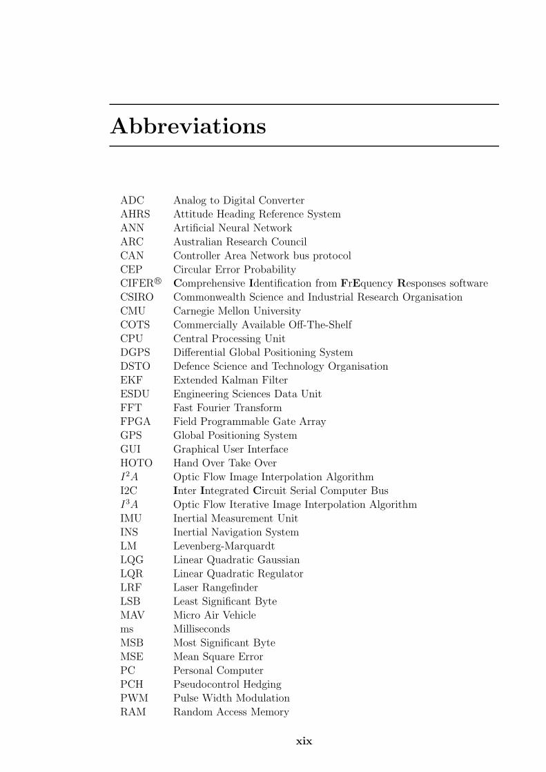
Abbreviations
ADC Analog to Digital Converter
AHRS Attitude Heading Reference System
ANN Artificial Neural Network
ARC Australian Research Council
CAN Controller Area Network bus protocol
CEP Circular Error Probability
CIFER R© Comprehensive Identification from FrEquency Responses software
CSIRO Commonwealth Science and Industrial Research Organisation
CMU Carnegie Mellon University
COTS Commercially Available Off-The-Shelf
CPU Central Processing Unit
DGPS Differential Global Positioning System
DSTO Defence Science and Technology Organisation
EKF Extended Kalman Filter
ESDU Engineering Sciences Data Unit
FFT Fast Fourier Transform
FPGA Field Programmable Gate Array
GPS Global Positioning System
GUI Graphical User Interface
HOTO Hand Over Take Over
I2A Optic Flow Image Interpolation Algorithm
I2C Inter Integrated Circuit Serial Computer Bus
I3A Optic Flow Iterative Image Interpolation Algorithm
IMU Inertial Measurement Unit
INS Inertial Navigation System
LM Levenberg-Marquardt
LQG Linear Quadratic Gaussian
LQR Linear Quadratic Regulator
LRF Laser Rangefinder
LSB Least Significant Byte
MAV Micro Air Vehicle
ms Milliseconds
MSB Most Significant Byte
MSE Mean Square Error
PC Personal Computer
PCH Pseudocontrol Hedging
PWM Pulse Width Modulation
RAM Random Access Memory
xix
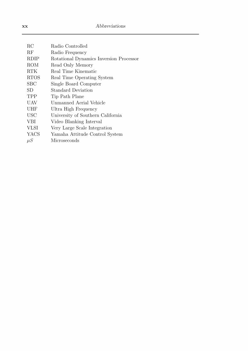
xx Abbreviations
RC Radio Controlled
RF Radio Frequency
RDIP Rotational Dynamics Inversion Processor
ROM Read Only Memory
RTK Real Time Kinematic
RTOS Real Time Operating System
SBC Single Board Computer
SD Standard Deviation
TPP Tip Path Plane
UAV Unmanned Aerial Vehicle
UHF Ultra High Frequency
USC University of Southern California
VBI Video Blanking Interval
VLSI Very Large Scale Integration
YACS Yamaha Attitude Control System
μS Microseconds
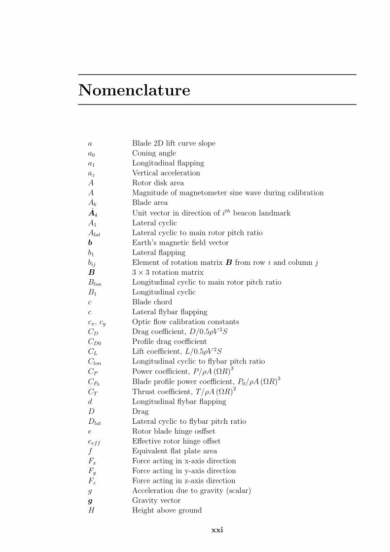
Nomenclature
a Blade 2D lift curve slope
a0 Coning angle
a1 Longitudinal flapping
az Vertical acceleration
A Rotor disk area
A Magnitude of magnetometer sine wave during calibration
Ab Blade area
Ai Unit vector in direction of ith beacon landmark
A1 Lateral cyclic
Alat Lateral cyclic to main rotor pitch ratio
b Earth’s magnetic field vector
b1 Lateral flapping
bij Element of rotation matrix B from row i and column j
B 3 × 3 rotation matrix
Blon Longitudinal cyclic to main rotor pitch ratio
B1 Longitudinal cyclic
c Blade chord
c Lateral flybar flapping
cx, cy Optic flow calibration constants
CD Drag coefficient, D/0.5ρV 2S
CD0 Profile drag coefficient
CL Lift coefficient, L/0.5ρV 2S
Clon Longitudinal cyclic to flybar pitch ratio
CP Power coefficient, P/ρA (ΩR)3
CP0Blade profile power coefficient, P0/ρA (ΩR)3
CT Thrust coefficient, T/ρA (ΩR)2
d Longitudinal flybar flapping
D Drag
Dlat Lateral cyclic to flybar pitch ratio
e Rotor blade hinge osffset
eeff Effective rotor hinge offset
f Equivalent flat plate area
Fx Force acting in x-axis direction
Fy Force acting in y-axis direction
Fz Force acting in z-axis direction
g Acceleration due to gravity (scalar)
g Gravity vector
H Height above ground
xxi
xxii Nomenclature
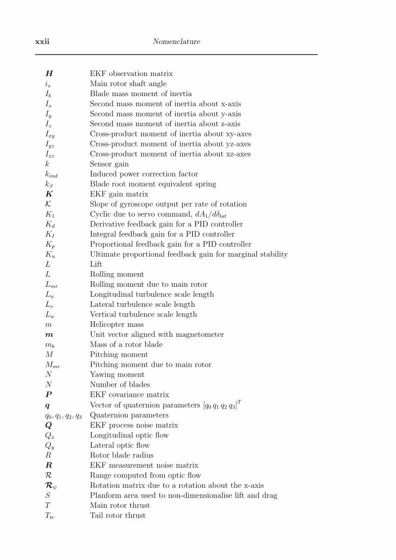
H EKF observation matrix
is Main rotor shaft angle
Ib Blade mass moment of inertia
Ix Second mass moment of inertia about x-axis
Iy Second mass moment of inertia about y-axis
Iz Second mass moment of inertia about z-axis
Ixy Cross-product moment of inertia about xy-axes
Iyz Cross-product moment of inertia about yz-axes
Ixz Cross-product moment of inertia about xz-axes
k Sensor gain
kind Induced power correction factor
kβ Blade root moment equivalent spring
K EKF gain matrix
K Slope of gyroscope output per rate of rotation
K1 Cyclic due to servo command, dA1/dδlatKd Derivative feedback gain for a PID controller
KI Integral feedback gain for a PID controller
Kp Proportional feedback gain for a PID controller
Ku Ultimate proportional feedback gain for marginal stability
L Lift
L Rolling moment
Lmr Rolling moment due to main rotor
Lu Longitudinal turbulence scale length
Lv Lateral turbulence scale length
Lw Vertical turbulence scale length
m Helicopter mass
m Unit vector aligned with magnetometer
mb Mass of a rotor blade
M Pitching moment
Mmr Pitching moment due to main rotor
N Yawing moment
N Number of blades
P EKF covariance matrix
q Vector of quaternion parameters [q0 q1 q2 q3]T
q0, q1, q2, q3 Quaternion parameters
Q EKF process noise matrix
Qx Longitudinal optic flow
Qy Lateral optic flow
R Rotor blade radius
R EKF measurement noise matrix
R Range computed from optic flow
Rψ Rotation matrix due to a rotation about the x-axis
S Planform area used to non-dimensionalise lift and drag
T Main rotor thrust
Ttr Tail rotor thrust
Nomenclature xxiii
u Longitudinal body-axis velocity
umean Mean longitudinal velocity
U Raw sensor output
v Lateral body-axis velocity
V Air velocity relative to TPP
Vi Rotor induced velocity
Vn Freestream velocity normal to TPP
VR Velocity of air relative to blade
Vt Freestream velocity tangential to TPP
w Vertical body-axis velocity
V∞ Freestream velocity
Vz Vertical velocity
X X position in Earth centred coordinates
Xb x body axis unit vector
Xg x global axis unit vector
W Vertical relative velocity between the ground and heliopter
Y Y position in Earth centred coordinates
Yb y body axis unit vector
Yg y global axis unit vector
zmr Vertical distance from main rotor hub to centre of gravity
Z Z position in Earth centred coordinates
Z Vertical position
Zb z body axis unit vector
Zg z global axis unit vector
Z Terrain clearance
α Blade section angle of attack
β Rotor blade flapping angle
δp Offset error of roll rate gyroscope
δq Offset error of pitch rate gyroscope
δr Offset error of yaw rate gyroscope
δx Offset error of x body axis accelerometer
δy Offset error of y body axis accelerometer
δz Offset error of z body axis accelerometer
δcol Collective pitch servo command
δlat Lateral (roll) servo command
δlon Longitudinal (pitch) servo command
δped Yaw servo command
δz Offset error of z body axis accelerometer
ΔT Time Step
γ Locke number, ρacR4/Ibγ2 CIFER R© correlation factor
ζix, ζiy, ζiz Sensor alignment coefficients for the ith sensor
θ Pitch angle
θ Blade incidence
xxiv Nomenclature
θmax Servo rate limit
θs Commanded sinusoidal servo amplitude
θ0 Blade collective pitch angle
κ Forward flight profile drag power correction factor
λ Rotor inflow ratio
λ Attitude vector correction factor
λx, λy, λz Components of Earth’s magnetic field along magnetometer axes
λi Rotor induced inflow ratio, Vi/ΩR
μ Rotor advance ratio
ρ Air density
σ Rotor solidity, Ab/A
σu Longitudinal turbulence intensity factor
σv Lateral turbulence intensity factor
σw Vertical turbulence intensity factor
τf Time constant of main rotor flapping
τs Time constant for flybar flapping
Υ Sensor offset
φ Roll angle
φ Phase angle of magnetometer sine wave during calibration
Φ Beacon elevation angle
Φ EKF fundamental matrix
ψ Blade azimuth angle measured anti-clockwise from above
ψ Yaw angle
ψ Rotation of IMU about an axes during calibration
Ψ Beacon azimuth angle
Ω Angular velocity of main rotor
Ωcr Servo corner frequency due to rate limit
Chapter 1
Introduction
1.1 Aim
The aim of this thesis is to investigate and develop an effective control system for a
flying vehicle using biologically inspired vision as the primary sensor. The underlying
motivation for this work is that it might make autonomy for Unmanned Aerial
Vehicles more practical in a real-world environment. This should be achievable
using cheaper and smaller vision based sensors to replace or augment sensors based
on Global Positioning Systems (GPS) and expensive Inertial Navigation Systems
(INS). In addition, vision potentially offers a better solution to the problem of
obstacle avoidance and terrain clearance than conventional techniques such as radar
or laser rangefinding.
Work in this thesis is confined to the control of helicopters in both hover and
forward flight. This is deliberately done as it increases the generality of the tech-
niques used, making them applicable to not just forward flight at high speed, but
also to vehicles attempting to operate in a confined region where motion may in-
volve occasionally stopping, flying sideways, vertically, turning on the spot or even
flying backwards. This makes the work more challenging owing to the additional
difficulties of controlling such a platform. Helicopters are dynamically unstable and
require constant external manipulation of the control inputs by a human or a ma-
chine pilot to prevent divergence from the desired flight path. Helicopter control is
highly non-linear due to the complex nature of the rotor aerodynamics. Helicopter
control channels are also highly coupled. For example, a commanded increase in
rotor thrust causes an increase in torque which must be compensated by application
of increased tail rotor pitch; this in turn requires a lateral tilt to the main rotor disk
to prevent sideways motion; this rotor tilt then needs to be offset by an increase in
thrust and a rotor longitudinal tilt to compensate for rotor flapping cross-coupling
effects.
1.2 Motivation
1.2.1 Unmanned Aerial Vehicles
Autonomous flying vehicles have many applications for operations in dangerous areas
where the risk to a human pilot would be unacceptable. Some examples include:
1
2 Introduction
mine detection and disposal, operations near a volcano and operations in radioactive
environments (e.g. dumping coolant on Chernobyl). They also have great potential
for applications such as search and rescue, exploration, crop dusting, interplanetary
exploration, survey, coastal patrol, pollution monitoring and atmospheric study.
Recent trends in modern warfare are showing an increased reliance on autonomous
flying vehicles to provide reconnaissance information and battlefield intelligence in
hostile environments. In April 2005, the New York Times [1] reported that the
number of UAVs in use in the skies over Iraq had exceeded 700. Such craft remove
humans from regions of potential danger and offer the hope of one day eliminating
humans from the battlefield.
1.2.2 Why vision sensing?
Laser Rangefinders (LRF) and radars both tend to be bulky which precludes them
from use on vehicles smaller than about 20kg. A typical LRF used for robotics is
the SICK LMS291 which weighs approximately 4.5kg [2]. The smallest Synthetic
Aperture Radar (SAR) planned for UAVs is likely to be the miniSAR from Sandia
Labs at 4-5kg [3]. By contrast, a self-contained device capable of measuring image
motion for terrain following has been produced by the Defence Science and Technol-
ogy Organisation (DSTO) which weighs less than 5 grams. The miniaturisation of
sensors will contribute to the practicality of Micro Air Vehicles (MAVs), classified as
aircraft with a wingspan of 15cm or less. MAVs could be used in a multitude of new
roles, benefiting from the low cost of manufacture and the difficulty of detection.
For military use, MAVs could be manufactured as a disposable item. The reduced
airworthiness regulatory requirements of MAVs makes them much easier to integrate
into the human environment since an MAV crash presents practically no risk to life
or property. The problem of fully integrating larger UAVs into civilian airspace is
still largely an unsolved problem and financial insurance for UAVs is hence difficult
to obtain for commercial operations.
The passive nature of a vision sensor provides many advantages over other forms
of ranging devices. Firstly, by not producing any electromagnetic emissions, a vision
sensor can be used in an operational environment where stealth is important, such
as on the battlefield or in a law enforcement situation. Secondly, there are health
risks associated with the use of radar and laser which need management. By using
a wide field of view, a camera also provides simultaneous ranging information over
a large area. Radars and laser rangefinders are essentially point sensors and need
to be scanned over the environment to build up a 3D map of the terrain. This
adds mechanical complexity or introduces the need for large antenna arrays to be
installed.
The most common navigation sensor used on UAVs is GPS. This is an appropri-
ate sensor for medium to high altitude aircraft flying away from terrain. However,
close to the ground, where terrain clearance must be maintained, GPS is only useful
when very detailed maps of the ground relief and other obstacles is held onboard.
In many cases this is not practical. In particular, when operating in urban environ-
ments, the obstacles to be avoided may be in motion such as cars and people. Vision
§1.3 Approach 3
provides an immediate observation of the environment and should be able to provide
a means of navigating through it which does not require a priori information about
the position of objects.
There is an increasing need for small UAVs to operate in urban cluttered envi-
ronments where GPS coverage cannot be guaranteed. Most accurate GPS imple-
mentations require at least 8 satellites to be observable in the sky. When flying
close to buildings, beneath underpasses and for indoor flight, this coverage will not
be achieved. One solution may be to augment GPS with visual sensing for parts
of the mission where GPS is not providing full accuracy. Alternatively, GPS would
be used to navigate a UAV into close proximity to a desired location before visual
guidance is activated to achieve high fidelity positioning near obstacles.
1.3 Approach
We learn from biology that it must be possible to build systems that are of small
size yet able to deal with complex environments. Many of the techniques used
by others in the related work section make use of feature matching and tracking
approaches which are difficult to achieve in repeated experiments due to changes in
environment such as varying lighting conditions. In this thesis, I have attempted
to search for ways to make the flight control system simple yet robust. Further I
have tried to apply biologically inspired vision to a more complicated and general
flight control problem than has been done before. Work by others on optic flow
sensing (see Chapter 2 for references) is mainly concerned with fixed wing aircraft,
ground robots and blimps which are either inherently stable or have such long time
constants in their motion that control stability becomes trivial.
As this thesis has progressed, the availability of new hardware has often su-
perceded work already completed. Initially, an off the shelf Hirobo Eagle helicopter
was adapted to autonomous operations by addition of sensors and a telemetry system
so that automated control could be executed from a ground-based computer. Later
developments in computer hardware and further competitive grant based funding,
permitted construction of an onboard processing system for another Eagle helicopter.
On these helicopters, all of the sensors were developed in-house including a series
of three-axis inertial measurement systems. The small payload capabilities of these
helicopters made miniaturisation of systems a primary concern. In 2004, through an
ARC Linkage grant, a Yamaha RMAX 90 kg helicopter became available. This he-
licopter had a much larger payload carrying capacity (30kg) and came with its own
inertial measurement system and convenient RS-232 based interfaces to controls and
telemetry. The longer endurance of the RMAX (1 hour compared to 15 minutes for
the Eagle) made the experimental side of the project much easier. For the purposes
of this thesis, the availability of the RMAX made much of the systems integration
work completed on the Eagle redundant. I have however persevered with the Eagle
architecture in parallel, to prove that the same concepts can be applied to a much
smaller rotorcraft with lower grade sensors.
Although the visual control in the thesis starts with fairly complex algorithms, I
4 Introduction
have been able to move to much simpler and less computationally intensive schemes
based on optic flow. The first visual guidance system used the more conventional
machine vision approach, involving the tracking of features on the ground with
detailed mathematics to resolve egomotion from the observed relative position of the
features. This method was found to be brittle and time consuming to implement.
The schemes based on optic flow were found to be much easier to demonstrate in the
field, owing to not having a reliance on feature tracking or complicated mathematical
processing.
1.4 Contributions
This thesis is primarily concerned with how to take processed visual sensor output
and use it in conjunction with the inertial sensors to control the flight path of a
helicopter. The thesis comprises the following key achievements:
• Development of a fully non-linear simulation of a small unmanned helicopter
and its sensors,
• A system for controlling a helicopter in hover using 3 visual landmarks on the
ground,
• Use of optic flow for controlling the longitudinal and lateral drift of a helicopter
attempting to hover over the ground without reference to any landmarks,
• The use of optic flow based ranging in forward flight to achieve terrain follow-
ing,
• The application of artificial neural networks to the control of a helicopter using
vision as the primary sensor, and
• An examination of new techniques for sensor fusion of inertial and visual in-
formation to produce estimates of attitude and velocity suitable for control of
the vehicle,
1.5 Layout of the Thesis
The thesis contains nine chapters. In Chapter 2, related work in the areas of visual
control of flight vehicles, calculation of optic flow and control techniques is presented.
Chapter 3 provides an overview of helicopter dynamics and details the implemen-
tation of a helicopter simulation for testing of control schemes and sensor fusion
used in the thesis. A detailed system description is provided for the helicopters
used in Chapter 4. Chapter 5 describes the experiments completed to control a he-
licopter in hover using vision as the primary sensor. The control of forward flight is
tackled in Chapter 6. Control schemes based on Artificial Neural Networks (ANN),
which reduce the mathematical complexity yet deal with the unmodelled helicopter

§1.5 Layout of the Thesis 5
dynamics are discussed in Chapter 7. In Chapter 8, advanced sensor fusion tech-
niques using Extended Kalman Filters are developed for combining the available
sensory inputs to provide useful variables for control. Finally, my conclusions and
recommendations for future work are provided in Chapter 9.

Chapter 2
Related Work
2.1 Introduction
This thesis project draws upon work from a number of diverse fields. I have struc-
tured my review of the related literature in terms of biologically inspired vision,
visual flight control, optic flow, sensor fusion and helicopter control.
2.2 Biologically Inspired Vision
This thesis was originally inspired by work done by Srinivasan et al [4–6] on the
mechanisms by which insects use optic flow to aid in navigation. Optic flow is the
motion of visual features across the field of view of the observer caused by translation
or rotation of the observer. Optic flow has various definitions in a machine vision
context, but is commonly described as the apparent motion of brightness patterns in
an image sequence [7]. Optic flow can be used to perceive relative range of objects
in the environment since close objects exhibit a higher angular motion in the visual
field than distant objects, when the observer is in motion.
A number of researchers e.g. [8–10] have suggested that insects in forward flight
perceive the range to objects in their field of view using optic flow. In [11], Srinivasan
theorises that insects use this process to maintain terrain and obstacle clearance by
effectively flying away from places in their field of view where angular motion is
high. This idea is at least 50 years old, and was put forward by Kennedy [12,13] as
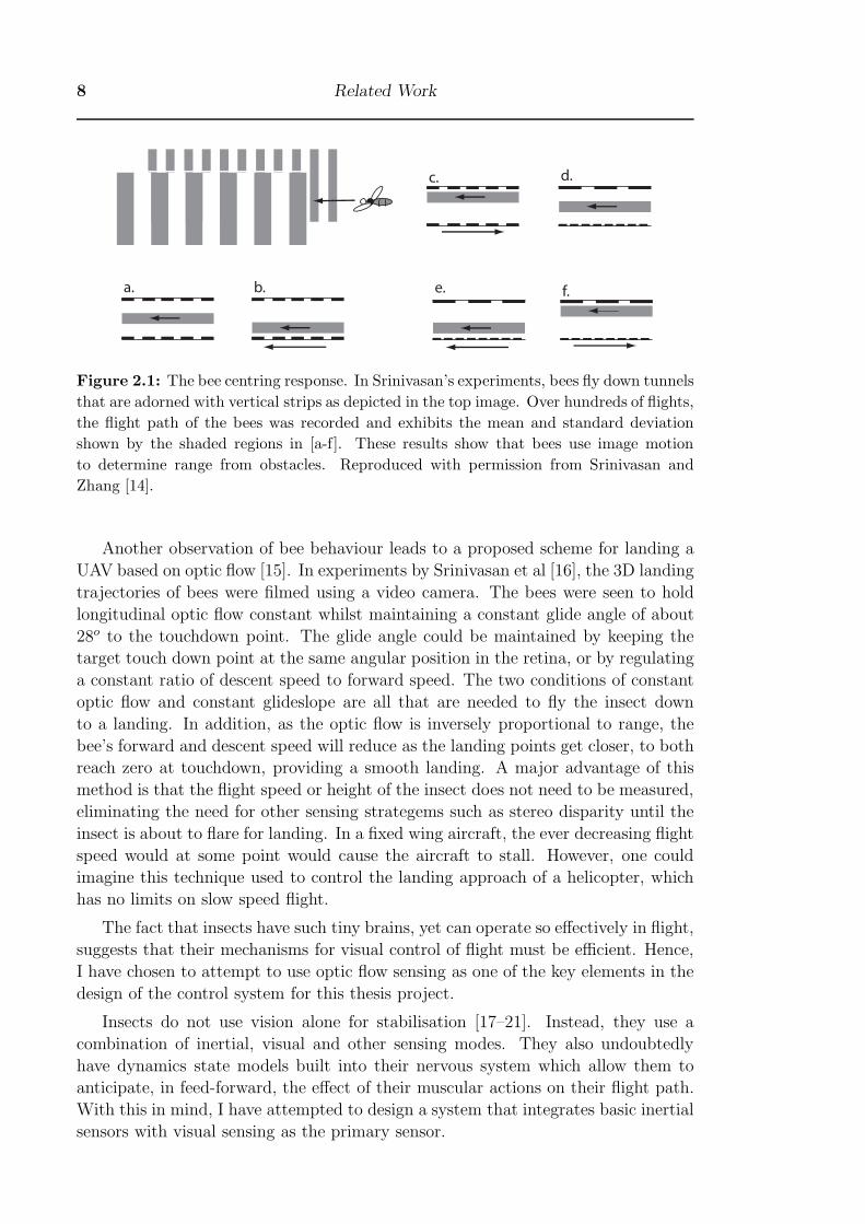
early as 1939. Through a series of experiments, Srinivasan and colleagues gathered
evidence for this idea based on the notion that bees use optic flow to centre their
flight path through narrow gaps. In the experiment, bees were trained to fly down
a tunnel. One of the walls of the tunnel was able to be moved longitudinally in
either direction using a conveyor belt arrangement. Averaged over many flights, a
very clear trend was that bees flying in the same direction as the moving wall flew
closer to the wall while bees flying in the opposite direction to the moving wall flew
further away. Further experiments demonstrated that this effect was not influenced
by the spatial period, intensity profile or contrast of the patterns placed on the
tunnel walls. Together, these experiments demonstrate that bees must judge their
distance from objects using the apparent angular speed of the environment. This
makes sense since it will provide a means of measuring range which is independent
of the visual texture of the environment, provided flight speed or height is known.
7
8 Related Work
c.
b. e. f.a.
d.
Figure 2.1: The bee centring response. In Srinivasan’s experiments, bees fly down tunnels
that are adorned with vertical strips as depicted in the top image. Over hundreds of flights,
the flight path of the bees was recorded and exhibits the mean and standard deviation
shown by the shaded regions in [a-f]. These results show that bees use image motion
to determine range from obstacles. Reproduced with permission from Srinivasan and
Zhang [14].
Another observation of bee behaviour leads to a proposed scheme for landing a
UAV based on optic flow [15]. In experiments by Srinivasan et al [16], the 3D landing
trajectories of bees were filmed using a video camera. The bees were seen to hold
longitudinal optic flow constant whilst maintaining a constant glide angle of about
28o to the touchdown point. The glide angle could be maintained by keeping the
target touch down point at the same angular position in the retina, or by regulating
a constant ratio of descent speed to forward speed. The two conditions of constant
optic flow and constant glideslope are all that are needed to fly the insect down
to a landing. In addition, as the optic flow is inversely proportional to range, the
bee’s forward and descent speed will reduce as the landing points get closer, to both
reach zero at touchdown, providing a smooth landing. A major advantage of this
method is that the flight speed or height of the insect does not need to be measured,
eliminating the need for other sensing strategems such as stereo disparity until the
insect is about to flare for landing. In a fixed wing aircraft, the ever decreasing flight
speed would at some point would cause the aircraft to stall. However, one could
imagine this technique used to control the landing approach of a helicopter, which
has no limits on slow speed flight.
The fact that insects have such tiny brains, yet can operate so effectively in flight,
suggests that their mechanisms for visual control of flight must be efficient. Hence,
I have chosen to attempt to use optic flow sensing as one of the key elements in the
design of the control system for this thesis project.
Insects do not use vision alone for stabilisation [17–21]. Instead, they use a
combination of inertial, visual and other sensing modes. They also undoubtedly
have dynamics state models built into their nervous system which allow them to
anticipate, in feed-forward, the effect of their muscular actions on their flight path.
With this in mind, I have attempted to design a system that integrates basic inertial
sensors with visual sensing as the primary sensor.

§2.3 Application of Visual Control to Robots 9
2.3 Application of Visual Control to Robots
Vision has been used to control robots since at least the early 1970s [22]. A number
of researchers have applied vision in control loops to ground-based robots using optic
flow [5, 23, 24] for collision avoidance. Other techniques that have been commonly
used in ground-based robots include stereo vision and target tracking.
During the life of this thesis project, visual control of UAVs has been a very
active area of research. Consequently, there have been a number of other groups
using similar approaches to mine which have published in the literature after I
completed the fundamental milestones of successful landmark tracking hover [25] in
2000 and optic flow controlled hover [26] in 2001. I have included the later work in
the following brief overview of progress in the field.
2.3.1 Biologically Inspired Visual Flight Control
For his PhD dissertation [27], Barrows developed a VLSI optic flow sensor for use
in a micro-UAV. The sensor consisted of a single chip sensor head containing photo
receptors and analog processing combined with a microcontroller that completed
the processing and output servo commands. The optic flow sensor was tested on a
small glider and used to avoid the floor and walls of an indoor hallway. The control
algorithm employed was ‘bang-bang’ in that if a certain threshold of optic flow was
exceeded, the aircraft elevator (or rudder) would be moved to a preset deflection.
In later work [28], optic flow sensors have been used outdoors by Barrows to control
the altitude of a small radio-controlled aircraft at altitudes ranging from 2 metres
to 10 metres.
In [29] a tethered 100 gram helicopter is described which used optic flow for ter-
rain following over an indoor circular track. The autopilot called OCTAVE (Optical
altitude Control sysTem for Autonomous VEhicles) was used to control a single
rotor mounted on a whirling arm. This arrangement constrained the rotorcraft to
flight in a circular path so that only one dimensional flow in the tangential direction
needed to be considered. The pitch of the rotor was adjusted by the operator to
set the desired speed of the helicopter. The height of the rotorcraft was controlled
by the autopilot by changing the speed, and hence thrust, of the rotor in response
to the perceived height over the terrain determined by optic flow. This technique
allowed the rotorcraft to maintain a relatively constant height over the terrain which
included a shallow ramp. In another experiment, the helicopter was able to land
by maintaining constant optic flow whilst the forward speed was reduced, a tech-
nique suggested by Srinivasan et al in [4]. For these experiments, the optic flow
was measured using a 1D Elementary Motion Detector (EMD) [30] inspired by the
physiological structure of a housefly’s visual system. The EMD circuit measured
the output of 20 photoreceptors arranged in a line and was implemented firstly on a
Field Programmable Gate Array (FPGA) [31] and later using a tiny microcontroller
to produce a sensor weighing less than one gram. In a related project, Zufferey [32]
used optic flow to control a number of robots. In Zufferey’s work, the output of
a 1D camera was processed by a PIC microcontroller to determine optical flow in
10 Related Work
one direction. The resulting optic flow computation was used to control a ground
vehicle and a small fixed wing aircraft. A number of behaviours were achieved:
• Steering control. Two 1D cameras, oriented at 45◦ from the forward axis,
were mounted on the fuselage of the fixed wing. The aircraft was flown inside a
large room and when optic flow on either camera exceeded a certain threshold,
the aircraft was turned by about 90◦ to avoid hitting a wall. The control was
achieved by smoothly applying rudder to full deflection and turning the aircraft
over a period of one second. Using this technique, the airplane was able to fly
four minutes without colliding with a wall.
• Simulated altitude control. A wheeled robot was used to maintain a con-
stant distance from a wall to simulate altitude control. By keeping optic flow
constant in a feedback loop, the robot maintained a relatively constant dis-
tance from the wall.
Reiser and Dickinson [33] describe object avoidance using optic flow in an insect-
inspired robotic control test bed comprising a 5 degree of freedom gantry. A vision
sensor comprising a 30 frame per second 115o x 95o field of view camera was placed
on the gantry and was free to move within a 92cm diameter cylindrical arena. A
PC attached to the sensor using a frame grabber was able to calculate optic flow
using an array of spatio-temporal correlation elements, using the method proposed
by Hassenstein and Reichardt [34]. For the experiments, the vertical position and
translational speed of the robot was kept constant and pitch and roll attitude was
kept fixed. Detectors for image expansion were used to trigger insect-like saccades,
such that the robot would rapidly change heading when approaching an obstacle.
The results showed that simple image loom detectors were enough to prevent the
robot from hitting the walls of the arena and obstacles placed inside the arena.
In [35,36] experiments were conducted on the AVATAR helicopter which suggest
that slow flying UAV may be able to avoid obstacles in an urban environment using
vision. For this experiment, the AVATAR was fitted with a forward looking stereo
camera and two cameras providing optic flow computation on the side. In forward
flight the sideways looking optic flow cameras determined range to objects in their
field of view. As the helicopter was flown towards obstacles on the side, such as
trees, the helicopter tended, in most instances, to turn away from those obstacles.
This technique might be extended to the point where a helicopter could safely pick
a path through an urban environment, such as flying down the middle of a street
autonomously.
Chahl tested a scheme for terrain following on a 1.2m wingspan delta-wing UAV
using optic flow [37]. For flight test, a downward looking camera with a field of
view of 100 degrees was used with a control-by-telemetry scheme implemented on a
500Mhz Pentium III ground computer. For each local optic flow vector calculated,
the scheme calculated the corresponding climb angle needed to clear the obstacle
represented by that flow vector. The maximum climb angle from the set of all
climb angles calculated was used as a reference input for the longitudinal controller.
Chahl noted that the rotational effect on the optic flow calculation dominates the
§2.3 Application of Visual Control to Robots 11
raw results, so that it is critical to subtract off the effect of rotations using a rate
gyroscope before calculating the range to obstacles.
2.3.2 Non-Biological Examples of Visual Flight Control
One of the earliest successful uses of vision to control a helicopter was undertaken
by Amidi for his PhD dissertation [38], submitted in 1996. In Amidi’s work, carried
out at Carnegie Melon University (CMU), a pair of cameras was used to track
natural features on the ground using high-speed template matching. The initial
features were selected by picking a window of pixels at the centre of the image. By
locking on to ground objects as the helicopter moves, the vision system was able to
estimate the helicopter’s position and velocity. Stereo vision was used to determine
the range to the features. A series of PD controllers were used in a feedback loop to
control the position of the helicopter in hover and slow forward flight. For outdoor
experiments, the vision system was implemented on a 67kg Yamaha R-50 helicopter
and was shown to be able to control the helicopter with a position accuracy of
3-10cm in hover.
Saripalli et al, at the University of Southern California (USC), have landed their
AVATAR autonomous helicopter on a helipad using vision and inertial information
[39]. The AVATAR is a small radio controlled helicopter with a PC-104 based avionic
architecture. In their work, a pattern comprised of polygons painted on the helipad
was detected and tracked so that the helicopter could align itself with the pattern
and then use its relative pose to land. The image was first segmented with a fixed
intensity threshold and then the first, second and third invariant moments of the
thresholded pixels were calculated and compared against a template descriptor of
the moments from the known target geometry (see [40] for an explanation of this
technique). The advantage of this approach is that the invariant moments are not
affected by translation, rotation or scaling and that the target descriptor is stored
as a relatively small vector. The helicopter was able to track the pattern even when
the helipad was moving, however, the helipad motion was stopped for the actual
landing.
In [41], Mejias et al worked with members from the USC group to achieve visual
servoing of the AVATAR and a similar small autonomous helicopter designated the
COLIBRI from the Universidad Politecnica de Madrid. The visual servoing target
was a window from a building. In the case of the COLIBRI, template matching based
on the Lucas-Kanade tracker [42] was used to match the image of the window being
tracked to a stored reference template of the window. This provided the coordinates
of the corners of the window which were used to generate a set of velocity commands
to an inner loop controller, to move the helicopter into a position where the target
was centred in the field of view. The helicopter was flown to within about 4m of the
window and then the visual servoing loop was activated. The helicopter trajectory
successfully converged to a position where the target was centred in the image.
Researchers at the University of California Berekely used a Yamaha R-50 un-
manned helicopter to test a vision system for control of landing [43, 44]. In this
work, a target comprising a black and white pattern of small squares of different
12 Related Work
sizes was placed on the ground. A camera image was first thresholded by using
a histogram technique with the intensity cuttoff set by trial and error. Once the
landing target was segmented from the background, the corners of the squares were
detected and each square was identified based on the centres of gravity. A non-linear
optimisation technique was used to calculate the position and attitude of the UAV
relative to the target. In their flight tests, the output of the vision algorithm was
compared to the output of the onboard GPS/INS system. The results compared to
within 5cm in translation and 5◦ in attitude.
Amongst other UAV programs, Georgia Tech operate a Yamaha RMAX UAV
dubbed the GTMax. This helicopter has been fitted with a variety of sensors in-
cluding differential GPS, inertial, magnetometers, an ultrasonic height sensor and a
camera. In their experiment, a target on the ground comprising a dark square on
a light background was tracked from a camera on the GTMax. Given the position
and orientation of the target apriori, an Extended Kalman Filter (EKF) was used
to fuse inertial data with data from the visual system, to provide the attitude and
position of the helicopter without GPS [45]. Using an EKF output as a reference,
the GTMax was able to follow position commands from the ground [46].
Proctor et al [47] constructed a glider with a camera and onboard video trans-
mitter which responds to commands telemetered from a control computer on the
ground. The guidance and control system used a high-speed pattern matching tech-
nique [48, 49] to track the outline of an open window using only a nose mounted
camera on the glider, with the aim of getting the glider to fly through the window.
A discrete EKF was used to estimate the states of the glider from the observed
window geometry. The results of simulation and flight test of the glider provided
an indication that, under some conditions, it would be possible to guide an aircraft
using vision alone.
2.4 Methods for Calculating Optic Flow
In selecting a method for calculating optic flow for my outdoor experiments, at-
tention was directed towards methods that are computationally efficient and fast
enough to be implemented in real-time on hardware small enough to be flown on-
board the helicopter. The methods had to be deterministic so that the execution
time never takes longer than the allocated time for processing within the control
loop (20 milliseconds). Finally, the method chosen had to be robust to noise so
that artifacts resulting from vibration, radio interference, dust and outdoor lighting
effects did not cause the method to fail.
Considerable work has been completed over the last three decades on developing
techniques for calculating optic flow robustly. The main approaches are correlation,
gradient models, energy methods and phase methods. An explanation of the classical
techniques can be found at [50]. A quantitative comparison of some of the best-
known techniques for calculating optic flow is provided by Barron and Beauchemin
in [51]. I will provide an overview of the main techniques described in the literature
before describing the image-interpolation technique used in this thesis.

§2.4 Methods for Calculating Optic Flow 13
2.4.1 Correlation
Correlation is probably the most obvious technique and involves matching image
regions or features between frames from different times. The objective is to find
the shift between two image regions, that correspond to the same features being
observed, which maximises some quantitative measure of similarity. The correlation
coefficient defined by the integral in Equation (2.1) is one such measure where f(x, y)
and g(x, y) are the intensities of the two frames being compared. Several types
of correlation measures are used including mean-normalised correlation, variance-
normalised correlation and sum of squared differences (SSD).∫ ∫f (x+ δx, y + δy) g (x, y) dx dy (2.1)
Anandan developed a hierarchical framework and algorithm for matching over-
lapping patches in an image [52]. Groups of pixels are compared with the surround-
ing pixel blocks to find the best match in terms of SSD to whole integer values of
pixel location. A quadratic approximation to the SSD surface centred on this pixel
location is then used to do a sub-pixel match. The search is conducted using a coarse
grid first which is used to guide the match at finer levels. A smoothness constraint is
used at each level of coarseness with a finite-element based minimisation technique
to find a smooth displacement field that approximates the displacements found from
the matching process.
Singh describes another two stage framework for computing image flow [53].
The first stage comprises a search strategy to find the best match between adjacent
patches to find local measurements of optic flow. The second stage combines the
velocity measurements for the pixels in a given image neighborhood using a Gaussian
weighting function which weights measurements from the centre of the neighborhood
more than those further from the centre.
Other correlation techniques are described in the literature including those by
Bulthoff et al [54]; Dutta and Weems [55]; Little and Kahan [56]; Burt et al [57];
and Glazer et al [58]. According to Barron [51], matching techniques tend to have
poor sub-pixel accuracy compared to other techniques such as gradient based meth-
ods. The correlation techniques can be robust but also tend to be computationally
demanding [59].
2.4.2 Gradient Methods
Gradient methods exploit the spatiotemporal gradients of image intensity to calcu-
late optic flow [60]. Gradient methods begin by assuming that the image intensity
is constant, which is a reasonable assumption provided that lighting conditions are
uniform and do not change suddenly, that specular reflections are small, shadows
are not present and surfaces are not translucent. Note that this assumption is also
required by most other optic flow methods [50]. With this assumption in place, the
intensity of a given point in the image f(x, y, t) does not change with time, so that
we can write:
14 Related Work
a b
b
c
c
a
V
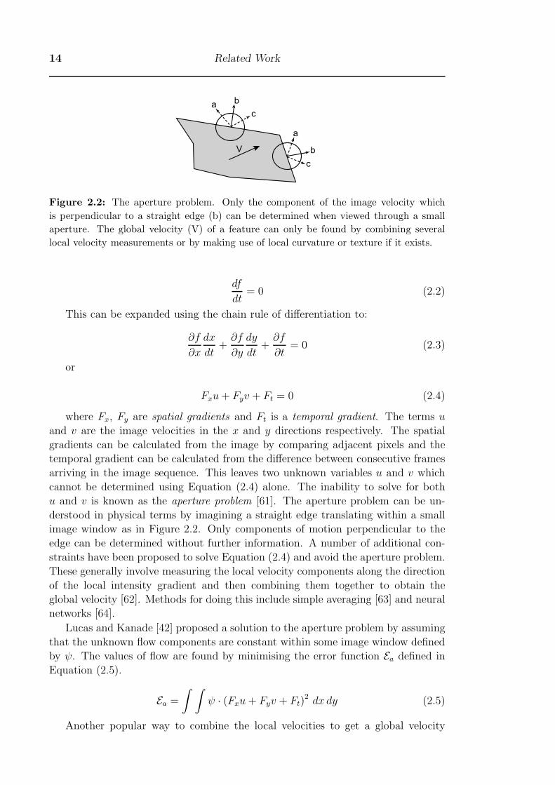
Figure 2.2: The aperture problem. Only the component of the image velocity which
is perpendicular to a straight edge (b) can be determined when viewed through a small
aperture. The global velocity (V) of a feature can only be found by combining several
local velocity measurements or by making use of local curvature or texture if it exists.
df
dt= 0 (2.2)
This can be expanded using the chain rule of differentiation to:
∂f
∂x
dx
dt+∂f
∂y
dy
dt+∂f
∂t= 0 (2.3)
or
Fxu+ Fyv + Ft = 0 (2.4)
where Fx, Fy are spatial gradients and Ft is a temporal gradient. The terms u
and v are the image velocities in the x and y directions respectively. The spatial
gradients can be calculated from the image by comparing adjacent pixels and the
temporal gradient can be calculated from the difference between consecutive frames
arriving in the image sequence. This leaves two unknown variables u and v which
cannot be determined using Equation (2.4) alone. The inability to solve for both
u and v is known as the aperture problem [61]. The aperture problem can be un-
derstood in physical terms by imagining a straight edge translating within a small
image window as in Figure 2.2. Only components of motion perpendicular to the
edge can be determined without further information. A number of additional con-
straints have been proposed to solve Equation (2.4) and avoid the aperture problem.
These generally involve measuring the local velocity components along the direction
of the local intensity gradient and then combining them together to obtain the
global velocity [62]. Methods for doing this include simple averaging [63] and neural
networks [64].
Lucas and Kanade [42] proposed a solution to the aperture problem by assuming
that the unknown flow components are constant within some image window defined
by ψ. The values of flow are found by minimising the error function Ea defined in
Equation (2.5).
Ea =
∫ ∫ψ · (Fxu+ Fyv + Ft)
2 dx dy (2.5)
Another popular way to combine the local velocities to get a global velocity
§2.4 Methods for Calculating Optic Flow 15
field is with a smoothness constraint which assumes that the flow velocities vary
smoothly between adjacent points in the image. For example, Horn and Schunk [65]
use a smoothness constraint based on minimising the square of the magnitude of
the gradient of the optical flow velocity E2c where:
E2c =
(∂u
∂x
)2
+
(∂u
∂y
)2
+
(∂v
∂x
)2
+
(∂v
∂y
)2
(2.6)
In Horn and Schunk’s method, the smoothness criterion and the sum of the errors
Eb in the image intensity equation are minimised simultaneously. A weighting factor
α is used to describe the relative weighting of these errors as in Equation (2.8). An
iterative scheme is then used to find the velocities which minimise the total error E .
Eb = fxu+ fyv + ft (2.7)
E2 =
∫ ∫ (α2E2
c + E2b
)dx dy (2.8)
Nagel [66] also uses a smoothness constraint but uses second order derivatives
to orient the smoothness constraint so that it is not imposed across steep intensity
gradients. This enables real-world images containing edges and occlusions to be pro-
cessed. Numerous other smoothness constraints have been proposed. Incorporation
of smoothness constraints are computationally intensive [62] and do not always lead
to the correct global velocities [67].
Lucas and Kanade’s technique is classified as a local method whilst techniques
using smoothness constraints are classified as global methods. The major drawback
of the local methods are that they do not overcome the aperture problem in parts
of the image where the image gradient is small [68], leading to sparse flow fields.
Global methods on the other hand provide denser flow fields but are thought to be
more sensitive to noise [51, 69].
Srinivasan developed a generalised gradient based algorithm [70] which addresses
some of the problems with gradient algorithms, namely deriving the correct global
velocity without first getting the local velocities and requiring higher order deriva-
tives. Srinivasan’s technique uses six spatiotemporal filters applied to the same
image patch. The size of the patch determines how local or global the resulting ve-
locities are. In later work [71], however, Srinivasan develops the Image Interpolation
algorithm and shows that it has better robustness and accuracy with a negligible
increase in execution time [72].
2.4.3 Energy methods
It has been suggested that some image motion properties are more evident in the
frequency domain [73, 74]. There is biological evidence to support the use of such
elements in nature [75]. Energy methods work by finding the energy peaks in the
spatiotemporal spectrum from a sequence of images. The term energy tends to be
used rather than power to be compatible with the spectrum involving coordinates in
16 Related Work
both time and space. Energies are calculated by means such as summing and squar-
ing of the outputs from the applied filters. Various combinations of spatiotemporal
filters of different orientation sensitivities are used to span the spectrum adequately.
Adelson and Bergen [76] explain that image motion presents itself as orientation
in space-time. They propose a concept using a series of spatiotemporal filters to
extract the orientation and hence the flow from the image. Heeger [75] points out
that the power spectrum of a translating two dimensional texture occupies a tilted
plane in the frequency domain. Using Gabor filters, Heeger presents results for an
optic flow algorithm based on extracting orientation.
Watson and Ahumada [73] use a combination of delays, temporal and spatial
filters to form sensors which are tuned to particular spatial frequencies and direc-
tions. Multiple sensors at different orientations and centred at different locations
in the image are used to determine a complete flow field. For testing Watson and
Ahumada’s sensors, 16 consecutive frames were required. This type of approach is
therefore computationally intensive [71]. Energy models can also be quite suscepti-
ble to variations in the contrast of image components [73].
2.4.4 Phase-Based Techniques
Phase based methods use the phase behaviour of band-pass filter outputs to measure
optic flow. Phase methods have the advantage of being able to cope with several
different velocities occurring on the same spatial patch, which would occur in the
case of changing occlusion and transparency. They are also more robust to noise
[74] than the amplitude-based energy methods discussed previously, owing to the
independence of phase from amplitude variations resulting from changes in lighting
conditions.
The use of phase dates back to the work of Hildreth [77]; Buxton and Buxton [78];
and Duncan and Chou [79]. In this early work, binary edge maps were generated
using various filters such as the Laplacian of a Gaussian which can be seen as finding
phase zero-crossings. Fleet and Jepson have provided a generalised treatment of the
use of phase information for optic flow in reference [74] in which the local optic flow
is computed from the motion of contours of constant phase. Their method uses
the output from a series of linear velocity tuned filters similar to the ones used by
Heeger [75].
2.4.5 Image Interpolation Technique
I have chosen to use Srinivasan’s Image Interpolation Algorithm [71], abbreviated
I2A, to compute optic flow resulting from the motion of a plane perpendicular to the
camera. The technique is non-iterative, does not require identification or tracking of
individual features in the image, and does not require the calculation of high order
spatial or temporal derivatives. These features make it robust to noise and quick to
execute. Of all the techniques reviewed, these properties make I2A most suited to
use for flight control.
Srinivasan discusses versions of the algorithm for any combination of translations
§2.4 Methods for Calculating Optic Flow 17
parallel to the plane with a rotation about an axis perpendicular to the plane. A
simplified version of the algorithm is also discussed which calculates the flow due to
pure lateral and longitudinal translation. For small rates of rotation, e.g. less than
about 10 degrees between consecutive frames, it is possible to accurately extract
translation signals at different parts of the image whilst neglecting the rotation
effects. For the work in this thesis, where optic flow is applied to the control of
hover and forward flight, the yaw rate of the helicopter is constrained by the tail
rotor control loop to be less than 0.1 degree per frame, hence, only the translatory
flow in various parts of the image needs to be considered. Furthermore, it is possible
to determine rotation from this flow field by looking at the distribution of translation
flow components in the image. This makes inclusion of the effects of rotation in the
algorithm of limited benefit, allowing us to dispense with the added computation
which is significant since the rotated reference images would need to be generated
using trigonometric functions. A simplified version of the algorithm is therefore used
which calculates the flow due to lateral and longitudinal translation only. A detailed
derivation of the I2A algorithm can be found in [71].
The algorithm compares the current image with a set of four reference images
which are translated from a previous frame. We define the pixel intensity functions
at times t0 and t as f0(x, y) and f(x, y) respectively where x and y are the image
coordinates measured in pixels. The reference images f1, f2, f3 and f4 are formed
from the first image by shifting them by reference shifts Δxref and Δyref pixels
along the x and y axes, so that Equation (2.9) applies.
f1(x, y) = f0(x+ Δxref , y)
f2(x, y) = f0(x− Δxref , y)
f3(x, y) = f0(x, y + Δyref)
f4(x, y) = f0(x, y − Δyref) (2.9)
The I2A algorithm relies on the assumption that the image at time t can be lin-
early interpolated from f0 and the reference images so that Equation (2.10) applies.
f = f0 + 0.5
(Δx
Δxref
)(f2 − f1) + 0.5
(Δy
Δyref
)(f4 − f3) (2.10)
Our objective is to calculate the translations Δx and Δy which give the best
match between the actual image f and the interpolated approximation f . We can
express this as a least square problem over an image patch defined by the window
function Ψ by minimising the error E where E is defined by Equation (2.12). The
two dimensional window function Ψ specifies the size and form of the patch. Gaus-
sian, triangular and boxcar kernels could be used, but the latter requires much less
computation time.
18 Related Work
E =
∫ ∫Ψ · [f − f ]2 dx dy (2.11)
=
∫ ∫Ψ · [f − {f0 + 0.5
(Δx
Δxref
)(f2 − f1) + 0.5
(Δy
Δyref
)(f4 − f3)}]2 dx dy
The error may be minimised by taking the partial derivatives of E with respect
to Δx and Δy and setting them to zero. After simplification, the two resulting linear
equations are at (2.12-2.13) can be solved simultaneously for Δx and Δy.
(Δx
Δxref
)∫ ∫Ψ · (f2 − f1)
2 dx dy +
(Δy
Δyref
)∫ ∫Ψ · (f4 − f3) (f2 − f1) dx dy
= 2
∫ ∫Ψ · (f − f0) (f2 − f1) dx dy
(2.12)
(Δx
Δxref
)∫ ∫Ψ · (f2 − f1) (f4 − f3) dx dy +
(Δy
Δyref
)∫ ∫Ψ · (f4 − f3)
2 dx dy
= 2
∫ ∫Ψ · (f − f0) (f4 − f3) dx dy
(2.13)
2.5 Helicopter Control
The last decade has seen a plethora of control techniques applied to unmanned
helicopters appear in the literature. My aim in reviewing this literature has been to
determine the most simple yet practical control system for a helicopter that would
allow demonstration of visual control. I have examined both classical, modern and
black-box control techniques.
2.5.1 Classical Control
The essence of classical control is successive feedback loop closure using linear control
elements such as Proportional (P), Integral (I), Derivative (D) and combinations of
these (e.g. PI for Proportional and Integral feedback). The gain of these controllers
can be tuned by trial and error, with empirical techniques such as those employed
by Ziegler and Nichols [80] or, in the presence of an accurate system model, using
tools such as root-locus [81] or frequency analysis [82, 83].
In Amidi’s work [84] with a Yamaha R-50 helicopter, the helicopter controller
was implemented as a series of PD controllers with output saturation. Single PD
controllers were used with the collective and tail rotor pitch servos to control height
and yaw respectively. The control of horizontal position and velocity was achieved
§2.5 Helicopter Control 19
with a series of three nested loops with two PD controllers in each loop for separate
control of the lateral and longitudinal channels. In the outermost loop, position er-
rors were used to control two reference velocities. In the middle loop, the reference
velocities were used as the input to the PD controllers for pitch and roll attitude
reference values. Finally the reference pitch and attitude values were used as in-
puts to the PDs controlling lateral and longitudinal cyclic. This system effectively
controlled the helicopter in hover to within 15cm.
Saripalli et al [39] implement a very similar control scheme to Amidi except in
their system a PI controller is used instead of a PD controller for control of alti-
tude and a simple proportional controller is used to control the inner loop attitude.
Mettler points out in [85] that the derivative feedback for the attitude inner loop
does not provide any advantage since the Bell-Hiller stabiliser bar fitted to most un-
manned helicopters already provides attitude rate feedback. Similar systems have
also been used by Buskey et al [86]; Sanders [87]; and Mettler et al [85].
Small-scale helicopters have faster dynamics than full-size helicopters which
makes them harder to control [88]. Most small helicopters designed for human
piloted control are therefore fitted with a mechanical stabilizer bar that provides
lagged attitude rate feedback to the main rotor, to improve stability. However, the
presence of a stabilizer bar complicates automatic control as it decreases the stabil-
ity margin for the coupled dynamic mode between the rotor and the fuselage. This
prevents high gain controllers from being implemented. Mettler et al [85] describe
the use of a notch filter in combination with a series of PD controllers to develop
an attitude controller for a Yamaha R-50 helicopter. The notch filter was set to the
natural frequency of the fuselage-rotor mode allowing the roll angle feedback gain
to be increased more than fivefold.
2.5.2 Modern Control Methods
The design of controllers using classical methods such as root locus and Bode meth-
ods is essentially trial and error [89]. The two concepts defining modern control are
that: (a) the design is based directly on the state-variable model and (b) perfor-
mance specifications are expressed in terms of a mathematically precise performance
criterion [90]. All the gains are solved simultaneously and are directly solved from
the state space matrix algebra. Modern controllers offer the prospect for improved
performance and can, in some cases, adapt to changing conditions. The downside of
most modern controller methods is that they require unmeasured states which can
be hard to accurately estimate. Whilst many modern control techniques are shown
to be closed loop stable and function on real helicopters, improvements in perfor-
mance over equivalent classical controllers on the same plant are rarely confirmed or
quantified in the literature. Furthermore, they may require accurate system models
which, in the case of a highly non-linear helicopter, may be difficult to achieve. It
is often stated that the use of PID control requires laborious tuning to take place.
Whilst this is true to some extent, the systems identification step required to de-
velop a modern controller is no less laborious and opens up many opportunities for
numeric error during the controller design stage. I have included a brief overview
20 Related Work
of the application of modern control theory to helicopter control for the sake of
completeness.
Many of the modern control techniques are linear methods. As the helicopter
is non-linear, linearisation of the system model is necessary in order to design a
working controller. Koo and Sastry present approaches to this based on differen-
tial flatness [91] and approximate feedback linearisation [92]. In these techniques,
approximate models are developed which are minimum phase, whereas the actual
plant being modelled is in fact non-minimum phase [93]. Unfortunately their work
was conducted in simulation models which ignore the rotor and actuator dynamics,
so successful performance on a real system is not guaranteed.
Optimal control is a branch of control theory that aims to find control laws to
maximise some optimality criterion. A typical optimality criterion involves a linear
quadratic form which serves to simultaneously minimise the control energy and the
time it takes the system to reach steady-state. Noting that the model has to be
linearised, and is therefore only an approximation of the real plant, it can be argued
that the condition of optimality can become somewhat invalid. Furthermore, the
choice of weighting factors used in the optimality criterion can become somewhat
arbitrary. Optimal controllers for helicopters have been proposed by Morris [94];
Mettler et al [95] and Bogdanov et al [96]. Morris et al tested a Linear Quadratic
Gaussian (LQG) controller [97, 98] on a small electric helicopter constrained to
moving in only pitch, roll and yaw. Even with this simplified system, the system
performance was not good, owing to unmodelled dynamics and the lack of angular
rate sensors. Mettler et al developed a successful LQG controller for the lateral-
directional dynamics of a small helicopter by ignoring the flapping dynamics and
treating the helicopter as a rigid body. Using a notch filter to attenuate the fuselage-
rotor mode, the controller was shown to successfully control bank angle in flight,
however removal of the notch filter resulted in instability.
Bogdanov et al describe State-Dependant Riccati Equation (SDRE) control [99]
of an X-cell 8kg RC helicopter and the Yamaha RMAX helicopter. The approach
consists of approximating the non-linear model with a linear set of state update
equations at each time step based on the current state. Treating the state equations
as linear, the Ricatti equation is then solved and used to calculate optimal control
inputs based on a linear quadratic cost function. Bogdanov’s results for trajectory
control of an RMAX flying a 183m× 183m square racetrack pattern are good with
a position accuracy of 2m and an altitude accuracy of about 1.2m. However, the
computational power required to solve the Ricatti equation is demanding, requiring
14ms out of 20ms at 50Hz on a 300MHz Pentium CPU to compute. This level of
processing could not be achieved on either of the systems used for this project as it
would have required an additional CPU to be added.
One method of dealing with inaccurate systems identification is to apply the
principles of robust control. In robust control methods, such as H2 and H∞ [100], the
objective is to ensure sufficient stability remains in all scenarios that could arise from
the presence of noise, disturbances and bounded uncertainties in the plant model. A
number of researchers have applied robust controllers to small helicopters. Takahashi
applied a H2 controller to a control of hover in a full-size helicopter simulator.
§2.5 Helicopter Control 21
Bendotti and Morris discuss a H∞ controller for a model helicopter constrained to
3 degrees of freedom only and show that it out performs an LQG controller [101].
Hashimoto et al develop and flight test a third order H∞ velocity controller for a
full-scale unmanned helicopter which augments an existing stability augmentation
system [102]. Other examples of H∞ techniques applied to helicopter control are
La Civita et al [103] ; Shim et al [93] and Yang et al [104–107]. Recent results
from test of a H∞ loop shaping controller on a Yamaha R-50 helicopter at CMU
have shown tracking performance which is claimed to exceed the performance of any
other techniques in the published literature [108]. On the basis of this result, one
would expect that H∞ would be a good candidate for future unmanned helicopter
control designs. However, this work was only made possible by the presence of a high
fidelity simulation model [103], so I have not pursued the approach in this thesis.
A number of schemes for controlling a helicopter using backstepping [109] have
appeared in the literature. Backstepping is a recursive technique whereby the com-
plete system is built up in cascaded stages, starting with a simple system that can
be stabilised using a known Lyapounov function. As each system is stabilised, an
integrator is added to the input and then the same process is repeated to design
a Lypanov function and feedback law to stabilise the new system. The process
continues until the complete system is stabilised. The advantage of backstepping
is that it can be applied to nonlinear system without having to make linearising
approximations. It also guarantees stability and can be made to be adaptive [110].
Mahoney and Hamel present simulation results for a robust trajectory tracking con-
troller using backstepping [111] which can enable a priori bounds on the tracking
performance to be set. A very similar approach is taken by Frazzoli et al [112] who
also develop a backstepping trajectory control in simulation. The disdavantage of
backstepping is that, even for simple systems, the algebra can become very compli-
cated and unwieldy. Hence, the currently published applications of backstepping to
helicopters tend to make a number of assumptions to simplify the models that are
unrealistic [113], such as assuming that the rotor can be manipulated to provided
instantaneous control forces and moments. For example the backstepping algorithm
by Mahoney et al [114] assumes that the flapping angles are directly measurable and
controllable, neither of which is practical. Whilst backstepping does show promise,
the complexity is not consistent with my stated aim of keeping the control systems
as simple and practical as possible.
2.5.3 Black-box Approaches to Control
The complexities and mathematical tedium of developing high-fidelity systems iden-
tification models of a plant can be avoided by using a black-box approach where no
assumptions are made about the internal structure of the plant. The two dominant
approaches for achieving this are fuzzy logic and Artificial Neural Networks (ANN).
Of these two, I have only pursued neural control because it has the greatest simi-
larity to the neural foundation of insect flight control, which is the inspiration for
this thesis. In addition, most of the work on fuzzy logic for helicopter control has
been tested in simulation only, whereas there are some encouraging results using
22 Related Work
ANNs that have been demonstrated on real helicopters. In some situations neural
networks and fuzzy logic can be shown to be equivalent.
Control based on fuzzy logic uses the concept of simultaneous membership in
various fuzzy sets. For example, if temperature feedback was being used in a control
system, the controlled variable might have a membership in both hot and warm
sets. As the temperature varies towards a state of being hot, the membership in
the hot set would increase whilst decreasing in the warm set. This approach allows
for smooth changes in parameters rather than the abrupt changes that would result
from using a simple threshold with binary logic. The advantage of fuzzy control
is that it can be built up from rules of logic that have physical meaning to the
designer, unlike neural networks for which the internal mechanisms can be difficult
or impossible to conceptualise.
The work on fuzzy logic control for helicopters dates back to the early 1990s
and has continued until present day. In 1995, Sugeno et al [115, 116] implemented
a set of 57 if-then type control rules for control of hover and slow speed flight on
a Yamaha R-50 helicopter. Jiang et al [117] designed a fuzzy logic controller to
adaptively cancel the errors in another controller which was based on approximate
inversion of a helicopter plant model. The controller was then tested on an AH-
64 Apache helicopter simulation. Sasaki et al [118] applied a learning fuzzy logic
controller to a linearised simulation of an RC helicopter in hover and showed that
it provided stable hover control. Amaral et al [119, 120] showed in simulation that
a neuro-fuzzy inference controller based on a combination of ANN and fuzzy logic
controllers could be used to control a Sikorsky S-61 full-size helicopter in hover.
Kadmiry and Driankov tested the use of fuzzy logic to schedule the gain for an
unmanned helicopter in a non-linear simulation [121,122]. In a non-linear simulation
for an X-Cell RC helicopter, Sanchez et al tested a combination of PID controllers for
control of attitude and altitude and fuzzy logic controllers for controlling translation
movement [123]. Other fuzzy logic controllers for helicopters have been tested in
simulation by Cavalcante et al [124] ; Phillips et al [125]; and Hoffmann et al [126].
2.5.4 Artificial Neural Networks
A neural network is a computational system comprised of interconnected processing
elements called neurons or nodes. Neural networks from the basis of mental function
in the brains of animals. Artificial neural networks (ANN) are a biologically inspired
paradigm for computing, implemented either in software or hardware. The idea of
using an ANN to perform computation was first proposed by McCulloch and Pitts
in 1943 [127].
The computational requirements for executing ANN (once trained) are generally
small and can be readily implemented for real-time control, making them suited to
implementation on a small robot where only modest computing resources may be
available. ANN can also be trained to perform a task without having to explicitly
model or understand the underlying dynamics. This is good for complicated systems
which may be unweildy or analytically non-tractable. ANNs can act as excellent
function interpolators, but cannot be relied on to extrapolate into regions where
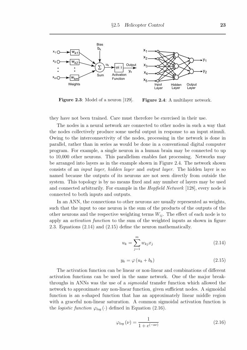
§2.5 Helicopter Control 23
Σ
wk1
wk2
wkm
Outputϕ(⋅)
yk
Bias
bk
Sum Activation
Function
uk
x1
x2
xm
Weights
Figure 2.3: Model of a neuron [129].
x1
x2
x3
x4
x5
y1
y2
InputLayer
HiddenLayer Layer
Output
Figure 2.4: A multilayer network.
they have not been trained. Care must therefore be exercised in their use.
The nodes in a neural network are connected to other nodes in such a way that
the nodes collectively produce some useful output in response to an input stimuli.
Owing to the interconnectivity of the nodes, processing in the network is done in
parallel, rather than in series as would be done in a conventional digital computer
program. For example, a single neuron in a human brain may be connected to up
to 10,000 other neurons. This parallelism enables fast processing. Networks may
be arranged into layers as in the example shown in Figure 2.4. The network shown
consists of an input layer, hidden layer and output layer. The hidden layer is so
named because the outputs of its neurons are not seen directly from outside the
system. This topology is by no means fixed and any number of layers may be used
and connected arbitrarily. For example in the Hopfield Network [128], every node is
connected to both inputs and outputs.
In an ANN, the connections to other neurons are usually represented as weights,
such that the input to one neuron is the sum of the products of the outputs of the
other neurons and the respective weighting terms Wij . The effect of each node is to
apply an activation function to the sum of the weighted inputs as shown in figure
2.3. Equations (2.14) and (2.15) define the neuron mathematically.
uk =
m∑j=1
wkjxj (2.14)
yk = ϕ (uk + bk) (2.15)
The activation function can be linear or non-linear and combinations of different
activation functions can be used in the same network. One of the major break-
throughs in ANNs was the use of a sigmoidal transfer function which allowed the
network to approximate any non-linear function, given sufficient nodes. A sigmoidal
function is an s-shaped function that has an approximately linear middle region
with a graceful non-linear saturation. A common sigmoidal activation function is
the logistic function ϕlog (·) defined in Equation (2.16).
ϕlog (ν) =1
1 + e(−aν)(2.16)
24 Related Work
In the various training algorithms that have been developed for ANNs, the ob-
jective is to adaptively change the weights in the internodal connections so that the
performance of the network is optimised. The most common methods for training
neural networks are supervised learning, unsupervised learning, and reinforcement
learning techniques. In supervised learning the network is provided with example
pairs of input data x and output data y from which it can learn a mapping between
the two. In unsupervised learning, the ANN is given the input data x but instead of
providing the desired outputs y, a cost function is provided, which is to be optimised
in some way. The cost function can be any function of the inputs and outputs. Re-
inforcement learning is similar to Unsupervised learning, except that the input data
is not provided beforehand, but generated by the interaction of the network with its
environment. In reinforcement learning, the network must learn by trying various
policies to optimise a reward signal provided to the network as a consequence of its
actions (outputs) [130].
After a period of dormancy in the 1970’s [129], neural networks underwent a
resurgence of interest following the publication of a book edited by McClelland and
Rumelhart [131] which outlined a method for training multi-layer ANNs using the
back-propogation algorithm. Backpropogation [132, 133] is a gradient descent tech-
nique designed to minimise the least square error between the ANN outputs and
the desired outputs. The training proceeds with a series of forward and backward
passes through the network using a set of training data. In the first pass, the out-
puts of the neurons are propogated forwards using Equations (2.14-2.15), starting
from the input side of the network, working through each layer in turn, until the
output layer is reached. In the forward pass the network weights are fixed. In the
second pass, the output errors are propogated backwards through the network and
used to adjust the network weights using an error-correction learning rule. As the
cycle is repeated for different training inputs and desired outputs, the weights of the
network gradually adapt to improve the match to the desired outputs. Whilst back-
propogation is well-known and easy to implement, it can be very slow to converge.
Other algorithms have been proposed which have much faster convergence for most
problems. The Levenberg-Marquardt (LM) algorithm [134] is renowned as one of
the fastest techniques for training ANNs with up to several hundred weights [135].
The LM algorithm was used for the work on ANNs in this thesis.
Certain kinds of ANNs can achieve temporal processing by making use of delayed
inputs. This allows ANNs to perform functions such as differentiation, integration,
filtering and state space representation of plant. A number of mechanisms for tem-
poral processing can be used, such as placing tapped delays on some of the inputs
to provide the network with a time history. The outputs of any layer can also be
passed back to the input layer. For example, the outputs of the hidden layer could
be passed back to the input layer through a tapped delay to provide a state-space
representation of the dynamics being modeled. Networks that have at least one feed-
back loop in their structure are known as recurrent networks, whereas feed-forward
neural networks do not feedback the output of any neuron to a pathway which can
affect the input of the same neuron. In this thesis, use is made of recurrent ANNs
to perform numerical integration for state-space propogation.
§2.5 Helicopter Control 25
2.5.5 Flight Control using Neural Networks
Teaching by Showing control for the attitude control of a small helicopter was demon-
strated in simulation by Montogomery and Bekey [136]. Their approach was to
augment a fuzzy logic controller with a neural network. The fuzzy logic controller
was implemented using a set of fuzzy rules relating angles and rate errors to roll
and pitch control inputs. The number and type of membership functions making up
the structure of the fuzzy controller were decided upon by a competent human pilot
based on their perceptions of how they flew a helicopter. A fuzzy learning algorithm
devised by Wang [137] was used to tune the fuzzy rule set as a teacher flew the heli-
copter. In practise, the teacher could be a human pilot, but in this case a non-linear
controller described in reference [138] was used. Once trained satisfactorily, the
fuzzy logic controller was activated and the teacher relinquished control. Whenever
the control performance fell below some criterion, due to changes in the system for
example, the trainer would take over control again and then a neural net would be
trained to predict the difference between the fuzzy controller and the trainer. Once
trained, the neural net output would then be used to augment the fuzzy controller
so as to better mimic the teacher. The combined fuzzy/ANN controller was found
to outperform the standalone fuzzy controller and provide stable control of attitude.
Buskey et al trained a simple feed-forward ANN with 10 hidden units to mimic
the actions of a human pilot [139]. The network inputs were accelerometer and rate
gyroscope outputs. For flight test, only the aileron servo was driven by the ANN
whilst the other servos were controlled by the pilot. The helicopter hovered for 15
seconds in this fashion until a wind gust necessitated the pilot taking over control.
The authors of this work attempted to use recurrent neural networks at first but
abandoned the attempt as no advantage was achieved from doing this with their
simple approach.
In 2001, Bagnell and Schneider demonstrated a reinforcement learning policy for
an autonomous helicopter [140]. In their scheme, a pair of very simple feed-forward
networks were used, comprising 5 weighted connections for each of the pitch and
roll control channels. The inputs to the roll channel network were lateral position,
lateral velocity and roll angle. Equivalent inputs were used for the pitch channel
which was treated as decoupled from the roll axis. A single hidden layer node was
used between the position input and the control output. The network functioned in
a similar fashion to a linear PD controller but the sigmoidal nature of the hidden
unit provided the ability to deal with large changes in the position set point. The
network weights were optimised using the amoeba technique outlined in [141] based
on various trajectories calculated in simulation. Cost functions which minimised the
velocities, position errors and control inputs were used. After proving the stability of
the resulting controller in simulation, the controller was tested on a R-50 helicopter
belonging to CMU. The helicopter was able to track moving position set points in
the presence of strong wind gusts.
In 2004, Ng et al published the results for a simple neural network controller
for a Yamaha R-50 helicopter using another reinforcement learning technique [142].
The approach was to first identify a non-linear 12 state model of the helicopter
26 Related Work
dynamics in hover. Next the PEGASUS reinforcement learning algorithm of [143]
was used to teach the ANN a policy for hovering in place. The inputs to the ANN
were the difference between the actual and desired helicopter state. The outputs
of the net were the cyclic pitch, collective pitch and tail rotor controls. The ANN
was structured so such that the lateral, longitudinal and vertical channels were
separated. For trajectory following, feed-forward between the yaw channel and the
other channels was also added. A quadratic cost function based on the control input
energy, velocities, orientation and the errors in position was used to optimise the
ANN weights. This technique was successful in not only hovering the helicopter, but
also in allowing it to follow trajectories, including a nose in circle and a rectangle
in the vertical plane. In later work [144], autonomous control of inverted hover was
successfully demonstrated using the same techniques.
Extensive work has been progressed at Georgia Tech to use neural networks to
augment other controllers. The aim of this approach is to reduce the reliance on
high-fidelity mathematical models when designing high-bandwidth controllers and to
allow the controller to adapt to changing environmental conditions. In 1994, Calise
et al published a scheme for adaptively correcting the inversion errors for an attitude
controller based on an inverted model of the helicopter attitude dynamics [145]. The
inverse controller known as the Rotational Dynamics Inversion Processor (RDIP)
takes as inputs the desired angular accelerations φ, θ and ψ and outputs the control
signals which it predicts should approximately accomplish these accelerations. The
desired angular accelerations were the output of PD controllers for roll, pitch and
yaw channels which were in turn driven by the output of a second order command
filter. Pilot commands were passed through the command filter to provide desired
outputs θd, θd,θd. The outputs used to generate a commanded angular acceleration
Uc using Uc = Kp(θc−θ)+Kd(θc− θ)+ θc where Kp and Kd are the gains of the PD
controller. The inversion model was a linear function of collective pitch angle, linear
velocities, angular rates and Uc. As the RDIP was based on a simple linear model
of the dynamics it contained errors owing to model uncertainty and the unmodelled
non-linearities. The ANN outputs were added to the desired angular accelerations
coming from the PD controllers to correct the inversion errors. A training scheme
based on the notion of Lyapunov stability and described in reference was used to
train the network online so that it could adapt to the inversion errors in flight [146].
When tested in a high fidelity Apache helicopter simulation, the controller was found
to track attitude commands much more precisely with the neural augmentation than
without it.
The work by Calise et al was extended by Leitner et al in 1998 to include a second
controller based on inversion which controlled the translational dynamics [147]. A
trajectory outer loop was built around the attitude inner loop and tested in simula-
tion. The outer loop uses an inverse dynamics block to calculate attitude commands
for the attitude controller. The inputs to the translational inverse dynamics block
were the desired linear accelerations which were calculated from the position/velocity
commands in a similar fashion to that used in the attitude command filter. The
translational inverse was a very simple analytic expression derived from considera-
tion of the desired tilt of the platform to obtain the desired accelerations. In 1999,
§2.5 Helicopter Control 27
Prasad et al published another application of this technique tested on an R-50 heli-
copter which implemented a rate control attitude hold (RCAH) function, by adding
an integrator to the commanded rate system [148].
In [149], Calise et al simulated R-50 pitch attitude control using the same neural
augmentation techniques with the addition of Pseudocontrol Hedging (PCH). PCH
was used to adjust the output of the command filter (i.e. the pseudocontrol) so
that the ANN did not see the actuator characteristics as model tracking error.
Actuators suffer from saturation and add high order dynamics and a pure delay
effect. The inverse model neglected the actuators and the neural network could not
adequately cope with effects such as saturation, so that the PCH was found to be
necessary to allow the ANN to adapt correctly. The 2nd order command filter was
also replaced by a 3rd order command filter as it better matched the dynamics of
the underlying system, dominated by the actuators. The new command filter and
the PCH gave much better results than previously attained. Other variations of this
approach were tested by Hovakimyan et al [150] who added a state space observer
to estimate the inversion errors and Corban et al [151] who added tapped delay lines
to the network inputs. In [152], Corban et al added an outer loop velocity controller
around the attitude loop already described and used a first order velocity filter to
convert the velocity commands from the pilot to pseudocontrol accelerations. PCH
was used to protect outer loop from adapting to inner loop dynamics. Using the
same control structure as Corban et al, Johnson and Kannan have obtained excellent
tracking results on the GTMAX unmanned helicopter [153]. These have included
precise tracking of racetrack, circular and square patterns in forward flight as well
as following a complex 3D trajectory previously flown by a human pilot and logged.
The ANN structure used in the neural augmentation work predominantly consisted
of two layers with five nodes in the hidden layer. The inputs to the ANN were the
full state and pseudocontrol error.
2.5.6 Controller Selection
Based on the literature, I have chosen to initially apply a classical helicopter con-
troller based on PID controllers and an attitude inner loop. This approach has been
shown to work on other small-scale helicopters and has a number of advantages over
other methods for experimentation. One such advantage is that the inner-loop can
be used as a stability augmentation system in the event of the outer loops being
deactivated or malfunctioning. The controller can be built up in stages with the
inner loop being designed and tested first. The inner loop also provides a bound on
the reference attitude used so that if the outer loop were to malfunction, the effect
on the helicopter can be constrained.
PID controllers are preferred because they are easily implemented and debugged,
can be readily tuned by trial and error and analysed without having a detailed plant
model. Whilst using the wrong gains can result in instability during tuning, this
can be overcome experimentally with a safety pilot. If the pilot is simultaneously
able to provide control inputs to augment the controller, gains can be gradually
ramped up until instability is reached and then backed off to provide desirable
28 Related Work
control performance.
Noting the biological parallels, I also intend to pursue the use of neural networks
for sensor fusion and control. There are many examples in the literature that show
that ANN can be used for flight control. ANN are computationaly efficient and can
easily be implemented with the hardware on the helicopter.
2.6 Summary
I have identified that visual control of an unstable rotorcraft is feasible. Based on
the biological observations, the use of optic flow would appear to be a very useful
sensing technique for control of flight, and I will aim to make use of this approach.
Noting its reported robustness and ability to be computed in real-time, I will use
the optic flow image interpolation algorithm (I2A) to calculate optic flow.
Chapter 3
Helicopter Simulation and Control
3.1 Introduction
The testing of new control and sensor algorithms is made practical for this thesis by
using a time domain simulation in SIMULINKR© of the helicopter dynamics, sensors
and controller. This allows the practicality of algorithms to be tested rapidly without
putting the helicopter at risk. The aim of the simulation is not to develop controllers
that can be copied directly from the simulation to the helicopter without further
tuning of control gains. Rather, the aim of the simulation is to determine what
style of controller can be used on the helicopter, taking into account the types of
sensors proposed. The simulation is also an excellent tool for developing sensor
fusion algorithms as in most cases the code can be transferred directly from the
simulation as a C file to the helicopter autopilot. For this thesis, a simulation of the
Eagle helicopter is used for all of the development work.
A number of other researchers have constructed simulations for small unmanned
helicopters. Munzinger [154] created a real-time hardware-in-the-loop (HIL) simula-
tion running on a Single Board Computer for a Yamaha R-50 unmanned helicopter.
The output of the simulation could be used to mimic the sensor data passed to the
actual onboard control system. Cunha and Silvestre [155] have developed a generic
helicopter dynamic simulation model and used this model to demonstrate an LQ
state feedback hover controller. Gavrilets et al developed and validated [156,157] a
HIL simulation under the QNXR© real-time operating system for their X-Cell 60size
helicopter. The Gavrilets simulation incorporated servo dynamics and sensor char-
acteristics and provided a good match with experimental data for a wide range of
conditions. Kowalchuk et al [158] created a 3 degree of freedom longitudinal dy-
namics model of their Raptor 50 sized helicopter, created within MATLAB R© with
a good match to flight data for pitch rate and pitch angle.
Mathematical models for small-scale helicopters have been extensively docu-
mented in the literature in recent years [94, 102, 159–161]. The general approach
is to combine a linearised rotor aerodynamic model with the non-linear rigid body
equations. Sometimes a non-linear thrust and rotor inflow model is incorporated,
usually involving an iterative scheme to simultaneously solve for the induced velocity
through the rotor and the thrust. The non-linear fuselage and tailplane aerodynam-
ics forces are only usually added when forward flight is considered. An underlying
theme in simulating small helicopters has been the realisation that owing to the
29
30 Helicopter Simulation and Control
complexity of the helicopter, minimum complexity simulations tends to be most
practical, so most researchers have chosen to use the minimum level of detail re-
quired to capture the key system dynamics. This approach was championed by
Heffley who published a report for NASA in 1988 on a minimum complexity heli-
copter model [162] that is regularly cited in the field. Heffley maintains that adding
higher order effects such as the off-axis moments due to blade flapping does not
automatically lead to a better match with flight data.
While hardware-in-the-loop models are very useful for specific platforms, a va-
riety of different platforms and sensor combinations have been used in this thesis,
so that the time spent writing interface code to mimic the data output protocols of
certain kinds of sensors would be prohibitive. SIMULINKR© was chosen as a devel-
opment environment for convenience as the graphical drag and drop building block
approach speeds up the development cycle and allows the simulation to be quickly
adapted to other helicopters. Balancing simulation fidelity against practicality, a
simulation has been created that is capable of simulating the following effects:
• Exact non-linear rigid body equations of motion;
• Wind gusts and turbulence;
• First order main rotor flapping dynamics;
• Hover, rearwards, sideways and forward flight;
• Dynamic effects of the Bell-Hiller stabiliser bar;
• Fuselage and tailplane aerodynamic forces;
• Approximate servo dynamics; and
• Sensor lags, filtering, offsets and noise.
The simulation does not model ground effect, interaction of rotor downwash with
the fuselage and rotor lead-lag mechanisms. Higher order flapping modes are only
really of interest when studying vibration and aeroelastic problems [163] so they
have also been ignored. Only low rates of descent are allowed on the helicopter so
that momentum theory can still be applied. This seems reasonable noting that all
of the experiments conducted for the thesis involve flight close to the ground so that
high descent rates cannot be achieved.
To simplify debugging, the simulation is divided into a number of blocks and
subsystems. On the highest level, the simulation consists of an aerodynamics sub-
system, sensor subsystem, sensor fusion block and controller subsystem as shown
in Figure 3.1. Diagrams of the internal structure of each subsystem are provided
in Appendix B. Most of the computational blocks have been implemented as C
code S-functions. In all, the base simulation consists of 19 C-files not including the
variety of blocks used later for testing sensor fusion algorithms and artificial neural
networks.

§3.2 Helicopter Dynamics 31
StateEstimator
Controller
states
Estimate
StateDisplay
ServoDynamics
State
Inertials
GPS
Optic Flow
Height
Position
Sensors
HelicopterDynamics
DesiredState
emu
Tail Rotor Pitch
Pitch Cyclic (B1)
Collective Pitch
Actual State
EstimatedState
Roll Cyclic (A1)
ServoCommands
Figure 3.1: Top level of eagle simulation
x
yz
Figure 3.2: Body axes system
3.2 Helicopter Dynamics
Having discussed the motivation for the simulation, a brief overview of the under-
lying theory is now provided.
3.2.1 Aircraft Conventions
The body axes system of the helicopter is fixed to the aircraft centre of gravity and
rotates as the aircraft’s attitude changes as shown in Figure 3.2. This set of axes is
particularly useful as the sensors are fixed with respect to the body axes. Another
set of axes, known as the inertial axes, are required for navigation and defined with
respect to the surface of the earth. The inertial axes are aligned so that the x-axis is
horizontal and points North, the y-axis is horizontal and points East and the z-axis
is positive down towards the centre of the earth. A precise mapping between the
inertial and body axes can be made based on the attitude of the helicopter.
Using standard aircraft nomenclature, the velocity components of the helicopter
along the body axes x,y and z are given the designations u,v and w respectively.
Likewise, the body axes rotation rates of the helicopter are p, q and r. The sense of
the rotations are defined in accordance with a right hand axes system.
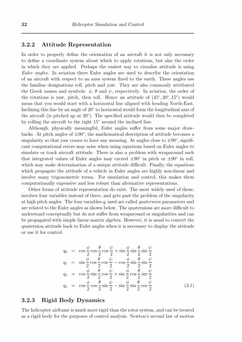
32 Helicopter Simulation and Control
3.2.2 Attitude Representation
In order to properly define the orientation of an aircraft it is not only necessary
to define a coordinate system about which to apply rotations, but also the order
in which they are applied. Perhaps the easiest way to visualise attitude is using
Euler angles. In aviation three Euler angles are used to describe the orientation
of an aircraft with respect to an axes system fixed to the earth. These angles use
the familiar designations roll, pitch and yaw. They are also commonly attributed
the Greek names and symbols: φ, θ and ψ, respectively. In aviation, the order of
the rotations is yaw, pitch, then roll. Hence an attitude of (45◦, 20◦, 15◦) would
mean that you would start with a horizontal line aligned with heading North-East.
Inclining this line by an angle of 20◦ to horizontal would form the longitudinal axis of
the aircraft (ie pitched up at 20◦). The specified attitude would then be completed
by rolling the aircraft to the right 15◦ around the inclined line.
Although, physically meaningful, Euler angles suffer from some major draw-
backs. At pitch angles of ±90◦, the mathematical description of attitude becomes a
singularity so that yaw ceases to have any meaning. At angles close to ±90◦, signifi-
cant computational errors may arise when using equations based on Euler angles to
simulate or track aircraft attitude. There is also a problem with wraparound such
that integrated values of Euler angles may exceed ±90◦ in pitch or ±90◦ in roll,
which may make determination of a unique attitude difficult. Finally, the equations
which propagate the attitude of a vehicle in Euler angles are highly non-linear and
involve many trigonometric terms. For simulation and control, this makes them
computationally expensive and less robust than alternative representations.
Other forms of attitude representation do exist. The most widely used of these,
involves four variables instead of three, and gets past the problem of the singularity
at high pitch angles. The four variables qi used are called quaternion parameters and
are related to the Euler angles as shown below. The quaternions are more difficult to
understand conceptually but do not suffer from wraparound or singularities and can
be propagated with simple linear matrix algebra. However, it is usual to convert the
quaternion attitude back to Euler angles when it is necessary to display the attitude
or use it for control.
q0 = cosφ
2cos
θ
2cos
ψ
2+ sin
φ
2sin
θ
2sin
ψ
2
q1 = sinφ
2cos
θ
2cos
ψ
2− cos
φ
2sin
θ
2sin
ψ
2
q2 = cosφ
2sin
θ
2cos
ψ
2+ sin
φ
2cos
θ
2sin
ψ
2
q3 = cosφ
2cos
θ
2sin
ψ
2− sin
φ
2sin
θ
2cos
ψ
2(3.1)
3.2.3 Rigid Body Dynamics
The helicopter airframe is much more rigid than the rotor system, and can be treated
as a rigid body for the purposes of control analysis. Newton’s second law of motion
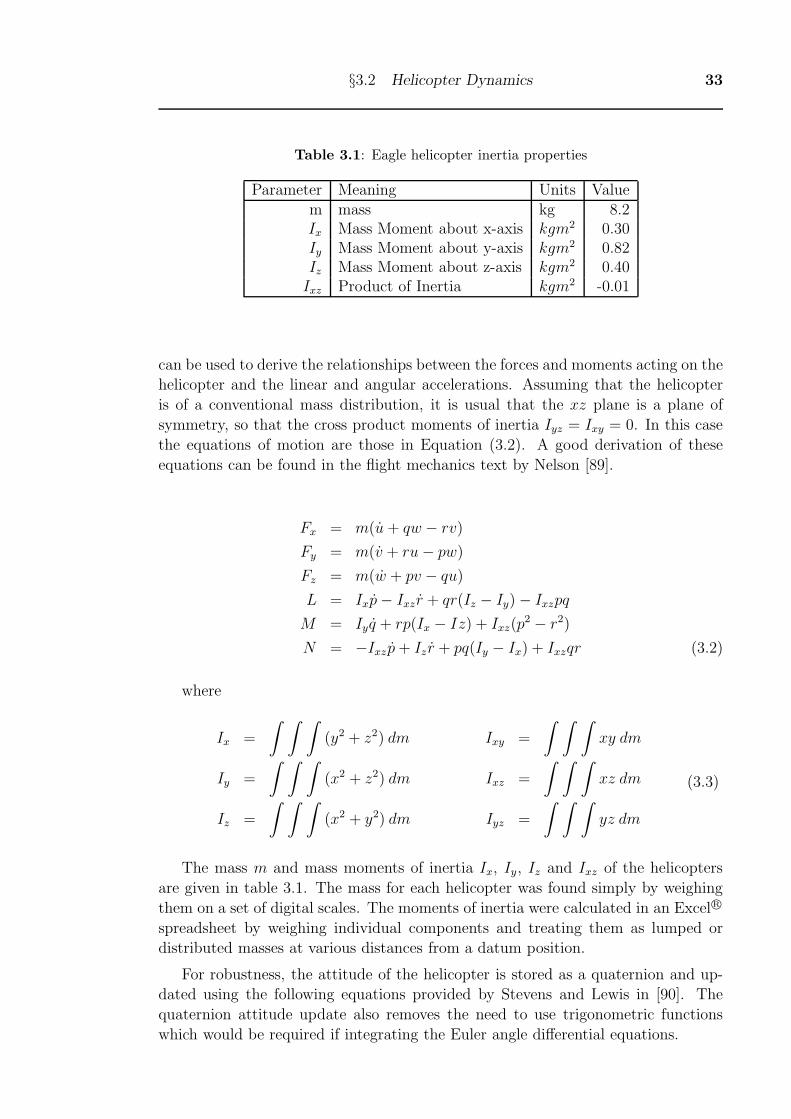
§3.2 Helicopter Dynamics 33
Table 3.1: Eagle helicopter inertia properties
Parameter Meaning Units Valuem mass kg 8.2Ix Mass Moment about x-axis kgm2 0.30Iy Mass Moment about y-axis kgm2 0.82Iz Mass Moment about z-axis kgm2 0.40Ixz Product of Inertia kgm2 -0.01
can be used to derive the relationships between the forces and moments acting on the
helicopter and the linear and angular accelerations. Assuming that the helicopter
is of a conventional mass distribution, it is usual that the xz plane is a plane of
symmetry, so that the cross product moments of inertia Iyz = Ixy = 0. In this case
the equations of motion are those in Equation (3.2). A good derivation of these
equations can be found in the flight mechanics text by Nelson [89].
Fx = m(u+ qw − rv)
Fy = m(v + ru− pw)
Fz = m(w + pv − qu)
L = Ixp− Ixzr + qr(Iz − Iy) − Ixzpq
M = Iyq + rp(Ix − Iz) + Ixz(p2 − r2)
N = −Ixzp+ Iz r + pq(Iy − Ix) + Ixzqr (3.2)
where
Ix =
∫ ∫ ∫(y2 + z2) dm
Iy =
∫ ∫ ∫(x2 + z2) dm
Iz =
∫ ∫ ∫(x2 + y2) dm
Ixy =
∫ ∫ ∫xy dm
Ixz =
∫ ∫ ∫xz dm
Iyz =
∫ ∫ ∫yz dm
(3.3)
The mass m and mass moments of inertia Ix, Iy, Iz and Ixz of the helicopters
are given in table 3.1. The mass for each helicopter was found simply by weighing
them on a set of digital scales. The moments of inertia were calculated in an ExcelR©
spreadsheet by weighing individual components and treating them as lumped or
distributed masses at various distances from a datum position.
For robustness, the attitude of the helicopter is stored as a quaternion and up-
dated using the following equations provided by Stevens and Lewis in [90]. The
quaternion attitude update also removes the need to use trigonometric functions
which would be required if integrating the Euler angle differential equations.
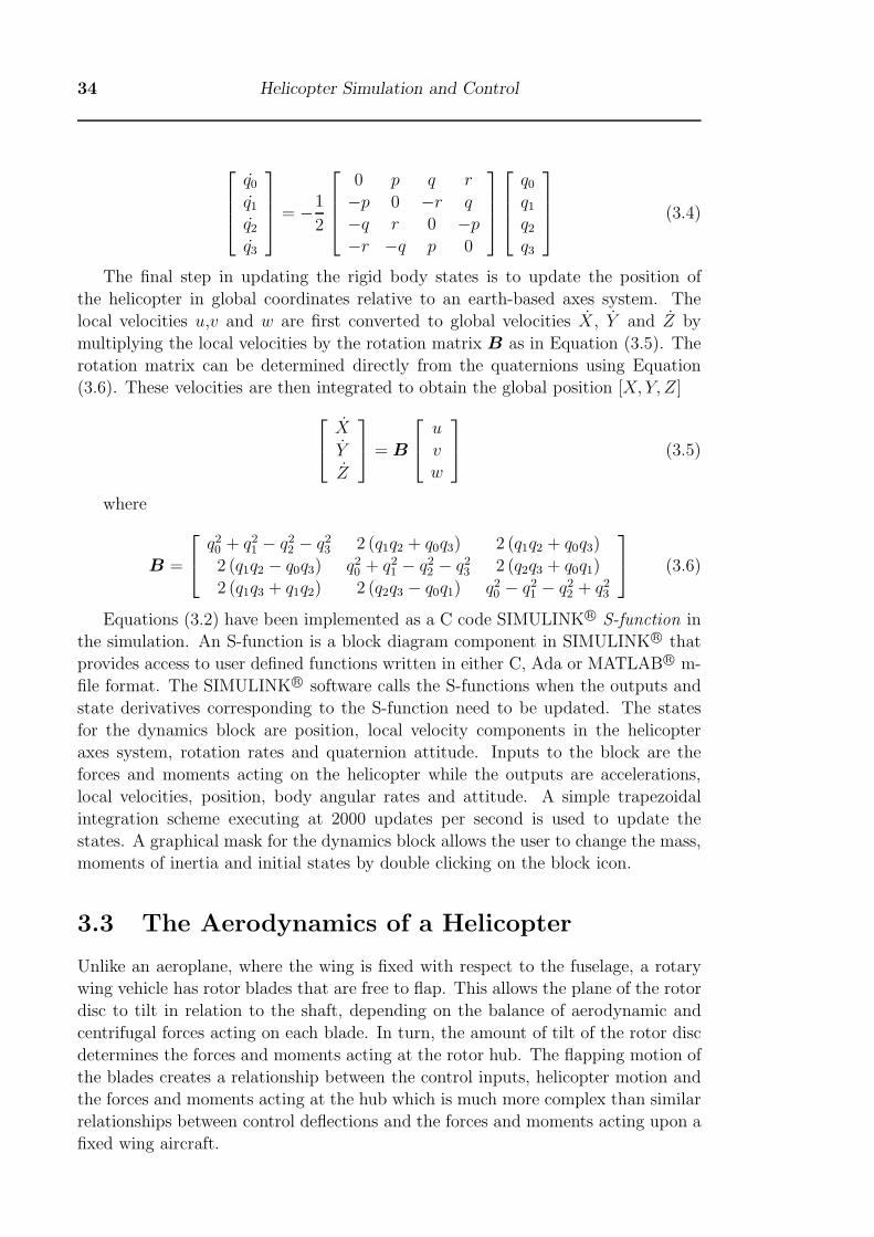
34 Helicopter Simulation and Control
⎡⎢⎢⎣q0q1q2q3
⎤⎥⎥⎦ = −1
2
⎡⎢⎢⎣0 p q r
−p 0 −r q
−q r 0 −p−r −q p 0
⎤⎥⎥⎦⎡⎢⎢⎣q0q1q2q3
⎤⎥⎥⎦ (3.4)
The final step in updating the rigid body states is to update the position of
the helicopter in global coordinates relative to an earth-based axes system. The
local velocities u,v and w are first converted to global velocities X, Y and Z by
multiplying the local velocities by the rotation matrix B as in Equation (3.5). The
rotation matrix can be determined directly from the quaternions using Equation
(3.6). These velocities are then integrated to obtain the global position [X, Y, Z]⎡⎣ X
Y
Z
⎤⎦ = B
⎡⎣ u
v
w
⎤⎦ (3.5)
where
B =
⎡⎣ q20 + q2
1 − q22 − q2
3 2 (q1q2 + q0q3) 2 (q1q2 + q0q3)
2 (q1q2 − q0q3) q20 + q2
1 − q22 − q2
3 2 (q2q3 + q0q1)
2 (q1q3 + q1q2) 2 (q2q3 − q0q1) q20 − q2
1 − q22 + q2
3
⎤⎦ (3.6)
Equations (3.2) have been implemented as a C code SIMULINKR© S-function in
the simulation. An S-function is a block diagram component in SIMULINKR© that
provides access to user defined functions written in either C, Ada or MATLABR© m-
file format. The SIMULINKR© software calls the S-functions when the outputs and
state derivatives corresponding to the S-function need to be updated. The states
for the dynamics block are position, local velocity components in the helicopter
axes system, rotation rates and quaternion attitude. Inputs to the block are the
forces and moments acting on the helicopter while the outputs are accelerations,
local velocities, position, body angular rates and attitude. A simple trapezoidal
integration scheme executing at 2000 updates per second is used to update the
states. A graphical mask for the dynamics block allows the user to change the mass,
moments of inertia and initial states by double clicking on the block icon.
3.3 The Aerodynamics of a Helicopter
Unlike an aeroplane, where the wing is fixed with respect to the fuselage, a rotary
wing vehicle has rotor blades that are free to flap. This allows the plane of the rotor
disc to tilt in relation to the shaft, depending on the balance of aerodynamic and
centrifugal forces acting on each blade. In turn, the amount of tilt of the rotor disc
determines the forces and moments acting at the rotor hub. The flapping motion of
the blades creates a relationship between the control inputs, helicopter motion and
the forces and moments acting at the hub which is much more complex than similar
relationships between control deflections and the forces and moments acting upon a
fixed wing aircraft.
§3.3 The Aerodynamics of a Helicopter 35
The controls of the helicopters used in this thesis are the same as a conventional
helicopter and consist of 5 control channels: collective pitch, lateral cyclic pitch, lon-
gitudinal cyclic pitch, tail rotor pitch and throttle. Observations of the RMAX and
Eagle helicopters with an optical tachometer have shown that the RPM does not
vary more than 1 percent during flight owing to onboard governors controlling the
throttle channel. For this reason the throttle channel has been ignored and a con-
stant RPM assumed. This simplification may not be appropriate during aggressive
manoeuvring.
The main rotor forces and moments are controlled by the collective and cyclic
pitch channels. The collective pitch control varies the average blade incidence of all
of the blades. Increasing the collective pitch control results in an increased angle of
attack of each blade and a subsequent increase in main rotor thrust. Decreasing the
collective pitch has the opposite effect. The vertical motion of the helicopter is thus
controlled by varying the collective pitch.
In order to achieve pitching and rolling moments, the orientation or tilt of the
rotor disk is changed by applying pitch that varies cyclically, once per revolution.
Increasing the blade pitch on one side of the rotor disk and decreasing it on the
opposite side causes the path of the blade tips, known as the Tip Path Plane (TPP)
to be tilted. Since the thrust vector acts essentially perpendicular to the TPP [164],
this can be used to change the trim of the helicopter. In addition to tilting the
thrust vector, moments acting at the rotor hub are generated by the effect of cyclic
pitch on the blade aerodynamic forces. Cyclic pitch is applied through a swashplate
comprising one fixed and one rotating plate joined by bearings. The servos are
connected to the fixed part of the swashplate as shown in Figure 3.6. The pitch
change links controlling the main rotor blade pitch are connected to the rotating
part of the swashplate so that tilting the swashplate causes the blade pitch to be
varied once per revolution in a sinusoidal fashion. Collective pitch can be achieved by
raising or lowering the swashplate to increase or decrease the blade pitch collectively.
The blade pitch θ can be described as the first three terms in a Fourier series as per
Equation (3.7) where ψ represents the azimuth angle of the rotor blade measured
anti-clockwise when viewed from above and starting with ψ = 0◦ at the tail. Note
that, as a general rule, blades may be twisted along their length, in which case the
blade pitch is also a function of radius. However for the Eagle, this is not the case.
In accordance with standard conventions [165], I will use the symbol θ0 for collective
pitch at the root of the blade and A1 and B1 for cyclic pitch.
θ = θ0 + A1 cosψ +B1 sinψ (3.7)
The variable A1 is known as lateral cyclic as it predominantly causes a rolling
moment while B1 is known as longitudinal cyclic as it results in predominantly a
pitching moment. The rotor control inputs are stimulated by three angular servos on
the Eagle which receive commands at 50Hz using Pulse Width Modulation (PWM).
Horns fitted to the shaft of each servo move to an angular position which is linearly
proportional to the width of the PWM pulse, with neutral servo angle being defined
as when the pulse width is 1.5 milliseconds. The angular displacements of the
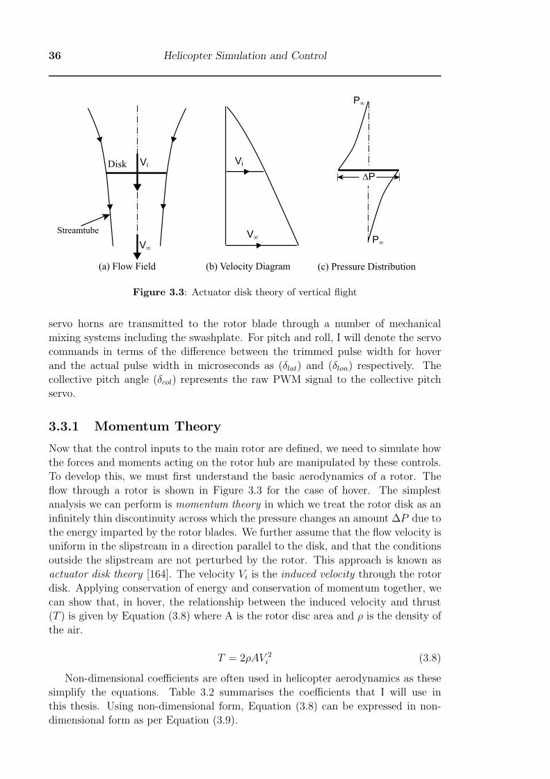
36 Helicopter Simulation and Control
Vi
V∞
Vi
V∞ P∞
P∞
ΔP
Disk
Streamtube
(a) Flow Field (b) Velocity Diagram (c) Pressure Distribution
Figure 3.3: Actuator disk theory of vertical flight
servo horns are transmitted to the rotor blade through a number of mechanical
mixing systems including the swashplate. For pitch and roll, I will denote the servo
commands in terms of the difference between the trimmed pulse width for hover
and the actual pulse width in microseconds as (δlat) and (δlon) respectively. The
collective pitch angle (δcol) represents the raw PWM signal to the collective pitch
servo.
3.3.1 Momentum Theory
Now that the control inputs to the main rotor are defined, we need to simulate how
the forces and moments acting on the rotor hub are manipulated by these controls.
To develop this, we must first understand the basic aerodynamics of a rotor. The
flow through a rotor is shown in Figure 3.3 for the case of hover. The simplest
analysis we can perform is momentum theory in which we treat the rotor disk as an
infinitely thin discontinuity across which the pressure changes an amount ΔP due to
the energy imparted by the rotor blades. We further assume that the flow velocity is
uniform in the slipstream in a direction parallel to the disk, and that the conditions
outside the slipstream are not perturbed by the rotor. This approach is known as
actuator disk theory [164]. The velocity Vi is the induced velocity through the rotor
disk. Applying conservation of energy and conservation of momentum together, we
can show that, in hover, the relationship between the induced velocity and thrust
(T ) is given by Equation (3.8) where A is the rotor disc area and ρ is the density of
the air.
T = 2ρAV 2i (3.8)
Non-dimensional coefficients are often used in helicopter aerodynamics as these
simplify the equations. Table 3.2 summarises the coefficients that I will use in
this thesis. Using non-dimensional form, Equation (3.8) can be expressed in non-
dimensional form as per Equation (3.9).
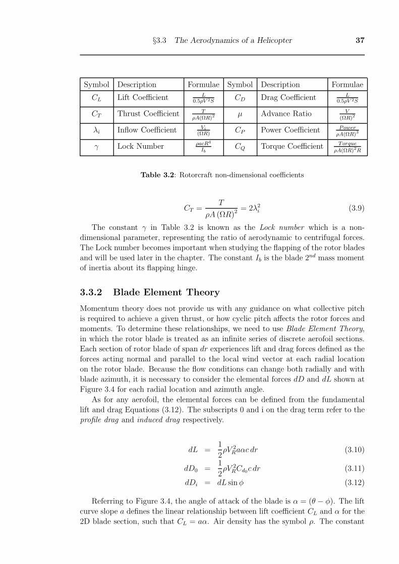
§3.3 The Aerodynamics of a Helicopter 37
Symbol Description Formulae Symbol Description Formulae
CL Lift Coefficient L0.5ρV 2S
CD Drag Coefficient L0.5ρV 2S
CT Thrust Coefficient T
ρA(ΩR)2μ Advance Ratio V
(ΩR)2
λi Inflow Coefficient Vi
(ΩR)CP Power Coefficient Power
ρA(ΩR)3
γ Lock Number ρacR4
IbCQ Torque Coefficient Torque
ρA(ΩR)2R
Table 3.2: Rotorcraft non-dimensional coefficients
CT =T
ρA (ΩR)2 = 2λ2i (3.9)
The constant γ in Table 3.2 is known as the Lock number which is a non-
dimensional parameter, representing the ratio of aerodynamic to centrifugal forces.
The Lock number becomes important when studying the flapping of the rotor blades
and will be used later in the chapter. The constant Ib is the blade 2nd mass moment
of inertia about its flapping hinge.
3.3.2 Blade Element Theory
Momentum theory does not provide us with any guidance on what collective pitch
is required to achieve a given thrust, or how cyclic pitch affects the rotor forces and
moments. To determine these relationships, we need to use Blade Element Theory,
in which the rotor blade is treated as an infinite series of discrete aerofoil sections.
Each section of rotor blade of span dr experiences lift and drag forces defined as the
forces acting normal and parallel to the local wind vector at each radial location
on the rotor blade. Because the flow conditions can change both radially and with
blade azimuth, it is necessary to consider the elemental forces dD and dL shown at
Figure 3.4 for each radial location and azimuth angle.
As for any aerofoil, the elemental forces can be defined from the fundamental
lift and drag Equations (3.12). The subscripts 0 and i on the drag term refer to the
profile drag and induced drag respectively.
dL =1
2ρV 2
Raαc dr (3.10)
dD0 =1
2ρV 2
RCd0c dr (3.11)
dDi = dL sinφ (3.12)
Referring to Figure 3.4, the angle of attack of the blade is α = (θ − φ). The lift
curve slope a defines the linear relationship between lift coefficient CL and α for the
2D blade section, such that CL = aα. Air density has the symbol ρ. The constant
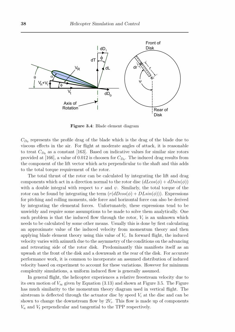
38 Helicopter Simulation and Control
θ
φ
α
dT
dL
φ
VR
dDo
Axis of Rotation
dDi
Vn
Vt
i+V ψ
dr r
Rear of
Disk
Front of
Disk
Figure 3.4: Blade element diagram
CD0represents the profile drag of the blade which is the drag of the blade due to
viscous effects in the air. For flight at moderate angles of attack, it is reasonable
to treat CD0as a constant [163]. Based on indicative values for similar size rotors
provided at [166], a value of 0.012 is choosen for CD0. The induced drag results from
the component of the lift vector which acts perpendicular to the shaft and this adds
to the total torque requirement of the rotor.
The total thrust of the rotor can be calculated by integrating the lift and drag
components which act in a direction normal to the rotor disc (dLcos(φ) + dDsin(φ))
with a double integral with respect to r and ψ. Similarly, the total torque of the
rotor can be found by integrating the term (r(dDcos(φ) +DLsin(φ))). Expressions
for pitching and rolling moments, side force and horizontal force can also be derived
by integrating the elemental forces. Unfortunately, these expressions tend to be
unwieldy and require some assumptions to be made to solve them analytically. One
such problem is that the induced flow through the rotor, Vi is an unknown which
needs to be calculated by some other means. Usually this is done by first calculating
an approximate value of the induced velocity from momentum theory and then
applying blade element theory using this value of Vi. In forward flight, the induced
velocity varies with azimuth due to the asymmetry of the conditions on the advancing
and retreating side of the rotor disk. Predominantly this manifests itself as an
upwash at the front of the disk and a downwash at the rear of the disk. For accurate
performance work, it is common to incorporate an assumed distribution of induced
velocity based on experiment to account for these variations. However for minimum
complexity simulations, a uniform induced flow is generally assumed.
In general flight, the helicopter experiences a relative freestream velocity due to
its own motion of V∞ given by Equation (3.13) and shown at Figure 3.5. The Figure
has much similarity to the momentum theory diagram used in vertical flight. The
airstream is deflected through the actuator disc by speed Vi at the disc and can be
shown to change the downstream flow by 2Vi. This flow is made up of components
Vn and Vt perpendicular and tangential to the TPP respectively.
§3.3 The Aerodynamics of a Helicopter 39
V 2∞ = u2 + v2 + w2 = V 2
n + V 2t (3.13)
Making small angle approximation for the flapping angles is justified since the
flapping angles rarely exceed 10o in normal flight [164]. Hence the expressions for
Vn and Vt are:
Vn = (a1 + is)u− b1v − w (3.14)
V 2t = u2 + v2 (3.15)
The most basic inflow assumption that can be made is to assume uniform inflow,
which is to say that the inflow Vi does not change with radius or azimuth. In this
case, we can integrate the elemental forces to achieve a closed form solution for
thrust in terms of collective pitch, inflow relative to the TPP (λ′) and advance ratio
(μ) as per Equation (3.16) (see [167] for a detailed derivation).
T =ρa (ΩR)2Ab
2
[1
3θ0
(1 +
3
2μ2
)− 1
2λ′]
(3.16)
where
λ′ =Vi + Vn
ΩRand μ =
VtΩR
(3.17)
3.3.3 Rotor Thrust
In order to calculate the inflow and hence thrust, use is made of Glauert’s induced
flow model [168] which likens a rotor in forward flight to an elliptically loaded fixed
wing of circular planform. This approach has been taken by several others [154,157,
162]. Based on the downwash for the equivalent wing, Glauert suggested that the
mean induced velocity Vi can be expressed as in Equation (3.18).
Vi =T
2ρAVwhere V =
√V 2T + (Vn + Vi)
2 (3.18)
Note that no theoretical basis exists for using the assumed flow pattern of Figure
3.5, other than: (a) in hover, Equation (3.18) reduces to Vi =√
T2ρA
which is the
momentum equation derived for axial flight; and (b) in fast forward flight V ≈ V∞and the formula becomes the same as that predicted for an elliptically loaded wing.
However there does appear to be a good match between this model and experiment
[167]. After some manipulation [165] of Equation (3.18) we can write:
V 2i =
√√√√( V2
)2
+
(T
2ρA
)2
− V 2
2(3.19)
The combination of momentum theory and blade element theory using Glauert’s
simple inflow model results in two coupled non-linear Equations (3.16) and (3.19)
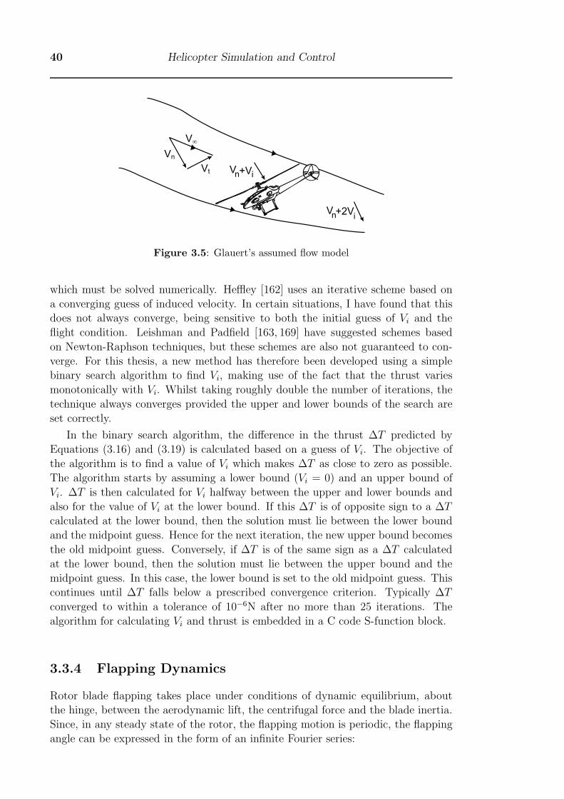
40 Helicopter Simulation and Control
V∞
Vn
Vn i+VVt
Vn i+2V
Figure 3.5: Glauert’s assumed flow model
which must be solved numerically. Heffley [162] uses an iterative scheme based on
a converging guess of induced velocity. In certain situations, I have found that this
does not always converge, being sensitive to both the initial guess of Vi and the
flight condition. Leishman and Padfield [163, 169] have suggested schemes based
on Newton-Raphson techniques, but these schemes are also not guaranteed to con-
verge. For this thesis, a new method has therefore been developed using a simple
binary search algorithm to find Vi, making use of the fact that the thrust varies
monotonically with Vi. Whilst taking roughly double the number of iterations, the
technique always converges provided the upper and lower bounds of the search are
set correctly.
In the binary search algorithm, the difference in the thrust ΔT predicted by
Equations (3.16) and (3.19) is calculated based on a guess of Vi. The objective of
the algorithm is to find a value of Vi which makes ΔT as close to zero as possible.
The algorithm starts by assuming a lower bound (Vi = 0) and an upper bound of
Vi. ΔT is then calculated for Vi halfway between the upper and lower bounds and
also for the value of Vi at the lower bound. If this ΔT is of opposite sign to a ΔT
calculated at the lower bound, then the solution must lie between the lower bound
and the midpoint guess. Hence for the next iteration, the new upper bound becomes
the old midpoint guess. Conversely, if ΔT is of the same sign as a ΔT calculated
at the lower bound, then the solution must lie between the upper bound and the
midpoint guess. In this case, the lower bound is set to the old midpoint guess. This
continues until ΔT falls below a prescribed convergence criterion. Typically ΔT
converged to within a tolerance of 10−6N after no more than 25 iterations. The
algorithm for calculating Vi and thrust is embedded in a C code S-function block.
3.3.4 Flapping Dynamics
Rotor blade flapping takes place under conditions of dynamic equilibrium, about
the hinge, between the aerodynamic lift, the centrifugal force and the blade inertia.
Since, in any steady state of the rotor, the flapping motion is periodic, the flapping
angle can be expressed in the form of an infinite Fourier series:
§3.3 The Aerodynamics of a Helicopter 41
β = β0 + a1 cosψ + b1 sinψ + a2 cos 2ψ + b2 sin 2ψ + . . . (3.20)
For most work, only the constant term and the two first harmonic terms are used.
The constant term represents the coning angle. The magnitude of the coefficients
dies off by approximately an order of magnitude for each harmonic, so that the
sin 2ψ and cos 2ψ terms are usually about 1/10th as significant as the sinψ and
cosψ terms. When only the first order terms are considered, the flapping angle β is
defined in terms of the coning angle a0, longitudinal flapping a1 and lateral flapping
b1 as per Equation (3.21).
β = a0 + a1 cosψ + b1 sinψ (3.21)
The flapping is affected by the cyclic pitch and also by the pitching and rolling
rates. Gyroscopic effects on the blade hinge moments result in coupling with the
rotation rates, which causes the TPP to lag behind the shaft when the aircraft is
pitching and rolling. For a typical helicopter, a pure pitch rate will generate a longi-
tudinal flapping effect which is about double the magnitude of the lateral flapping.
This is a source of cross-coupling known as rate cross coupling. However, Heffley
suggests that the rate cross-coupling be ignored, as it does not necessarily produce
a good match to flight data. Prouty [165] derives a rather complex expression for
the effect of the rotation rates in terms of the hinge offset, advance ratio and other
constants. For low speed and zero hinge offset, this simplifies to Equations (3.22-
3.23).
a1 = −16
γ
( qΩ
)+( p
Ω
)(3.22)
b1 = −16
γ
( pΩ
)−( q
Ω
)(3.23)
Tischler and Remple [170] show that the main flapping of the main rotor, which
is a second order systems, can be accurately represented as two coupled first order
equations. If the cross-coupling terms are initially ignored as suggested by Heffley
[162], these equations become those in Equations (3.24-3.25).
a1 = −q − 1
τf
(a1 +
da1
dB1
B1
)(3.24)
b1 = −p− 1
τf
(b1 +
db1dA1
A1
)(3.25)
For a teetering rotor, consisting of a rotor blade hinged on the axis of the shaft,
it can be shown that the natural frequency of the flapping is equal to the angular
velocity of the rotor Ω. As the system is therefore in resonance, the phase lag
between the excitation (the once per revolution cyclic pitch) and the flapping is
exactly 90◦. The Eagle main rotor hub consists of a pivot on the shaft axis about
42 Helicopter Simulation and Control
which the blades can flap and an elastomeric element that allows moments, as well
as forces, to be transferred from the rotor blade to the hub. The arrangement can
be conceptualised as the combination of a moment from a centre spring and a tilted
TPP [157] as shown in Figure 3.7. A consequence of the centre spring is that the
natural frequency of the rotor blade flapping is no longer in resonance with the
rotational excitation, leading to a reduced phase shift between flapping and cyclic
pitch and a decreased flapping time constant. Prouty [165] derives the time constant
for flapping of a hinged rotor blade to arrive at Equation (3.26) in terms of the hinge
offset from the shaft. The time constant is typically between one-quarter and one
half of a rotor revolution, depending on the effective hinge offset and spring constant.
τf =16 (1 − e/R)
γΩ (1 − e/R)4 (1 + e/3R)(3.26)
Cooke [171] shows that the effect of a spring on the rotor blade hinge is equivalent
to the effect of hinge offset and goes on to derive equations for the effect of the spring
on the natural frequency and damping ratio. Re-arranging Cooke’s equations which
deal with both hinge offset and spring constant, provides Equation (3.27) which
allows the effective hinge offset eeff to be calculated.
eeff =Kβ
mbrgR2Ω2(3.27)
where Kβ is the spring stiffness, mb is the mass of the blade and rg is the radial
location of the centre of gravity of the blade. Substitution of the effective hinge
offset back into Equation (3.26) provides a means to calculate the time constant.
For the case of the Eagle, this results in an effective hinge offset of e = 0.12 and a
flapping time constant of approximately 6 milliseconds.
One other important effect on flapping needs to be considered. A helicopter rotor
responds to changes in sideslip through an effect well-known for fixed wing, dihedral
effect. The effect of dihedral is for the helicopter to roll away from sideslip. This is
a stabilising influence which acts to maintain wings level, since a bank to one side
results in the aircraft sideslipping towards the low wing. The resulting sideslip and
dihedral effect then causes the aircraft to roll away from the low wing. Consider
a hovering helicopter with blades rotating anti-clockwise. If a helicopter were to
suddenly experience a gust from the right, the rear of the disk would be advancing
into the flow and generate increased lift. Blades at the front of the disk would be
retreating from the relative wind and receive a net decrease in lift. Due to phase lag,
the TPP would be tilted to the left and the helicopter would get a rolling moment to
the left, rolling the helicopter away from the gust. I make use of Heffley’s equation
for dihedral effect (3.28) which is provided at [162]. Since the thrust coefficient does
not change greatly between hover and forward flight, its value is calculated once at
the start of the simulation based on the thrust coefficient for steady hover.
db1dv
=da1
du=
2
ΩR
(8CTaσ
+
√CT2
)(3.28)

§3.3 The Aerodynamics of a Helicopter 43
Flybar
Paddle
Swashplate
Servos
R1
Shaft
R2
L1 L2
L3
RotorBlade
Fixed Plate
Rotating PlateBell-HillerMixing Lever
Figure 3.6: Flybar arrangement with Bell-Hiller stabilisation system
The main rotor flapping is implemented as a discrete S-function block in SIMULINKR©.
The inputs to the block are the velocities (for dihedral effect), the rotation rates for
calculation of gyroscopic effects and the cyclic pitch. The outputs of the block are
the longitudinal and lateral flapping angles, a1 and b1.
3.3.5 Flybar Dynamics
A feature of practically all small unmanned helicopters is a control rotor, known
as a flybar, which augments the stability of the main rotor. The flybar is a hybrid
of stabilising arrangements patented by Bell and Hiller. The primary effect of the
flybar is to provide feedback from the helicopter pitch and roll rates to the cyclic
pitch of the blades. The time constant of the flybar is much lower than for the main
rotor which slows down the dynamics of the helicopter, making it easier for a human
pilot to fly. A number of groups have provided an analysis of the flybar with varying
degrees of complexity [172]. All of the UAV platforms utilised for this thesis project
employ a flybar arrangement consisting of a teetering rotor rotated 90 degrees out
of phase with the main rotor. The flybar blades comprise small paddles which are
connected to the main rotor pitch change horns through a Bell-Hiller mixing lever
as shown in Figure 3.6. The incidence of the paddles is controlled by linkages to the
swashplate (not shown in the figure).
Unlike the Hiller stabiliser bar, the flapping angle of the flybar is used to control
the main rotor blade pitch. Application of cyclic pitch causes the flybar pitch to
change, resulting in flapping of the flybar. The flapping of the flybar is fed through
mechanical linkages to adjust the main rotor blade cyclic pitch, resulting in the
TPP tilting as desired. This scheme introduces significant lag into the control loop,
which would be problematic for the pilot, so that some cyclic pitch is fed through a
mechanical mixing system directly into the main rotor to provide some faster control.
The flybar is hinged at the shaft so that the time constant Equation (3.26) simplifies
to Equation (3.29). For the Eagle, the time constant of the flybar is approximately
0.23 seconds which is significantly slower than that for the main rotor.
44 Helicopter Simulation and Control
τs =16
γsΩ(3.29)
The flapping (βs) of the flybar is defined by the longitudinal flapping c and the
lateral flapping d such that βs = c cosψ + d sinψ. A set of first order Equations
(3.30) defines the flapping dynamics. The constants Dlat and Dlon represent the
gearing ratio between the servo commands δlat and δlon and the corresponding pitch
change of the flybar paddles.
τsd = −d− τsp+Dlatδlat
τsc = −c− τsq + Clonδlon (3.30)
The linearised relationship between the cyclic pitch fed to the main rotor blades,
the flybar flapping and the servo commands are presented in Equation (3.32). The
constants Alat, Blon and Ks represent the combined gain of the servos and the
mechanical mixing ratios of the linkages. The values of the constants Alat and
Blon were found by measuring the variation in pitch with variation in the control
signal sent to the servos. The value of the constant Ks was estimated based on the
kinematics of the linkage geometry. For the purposes of simulation, the mechanical
mixing equation was treated as linear, although some non-linearity does exist. The
flybar dynamics are implemented in their own S-function block. Inputs are the
rotation rates and cyclic pitch. Outputs are the flapping which is fed to the input
of the main rotor flapping block.
A1 = Alatδlat +Ksd (3.31)
B1 = Blonδlon −Ksc (3.32)
3.3.6 Main Rotor Control Forces and Moments
The longitudinal and lateral forces and moments acting on the main rotor hub are
a result of tilting the TPP. Referring to Figure 3.7, it can be seen that the effect
of the centre spring is to create a moment to be transferred to the rotor hub which
is linearly proportional to the flapping angle β. The stiffness of the centre spring
acting on the Eagle rotor hub, was measured in a force deflection test and found to
be Kβ = 270 Nm/radian. The TPP tilt also causes the thrust vector to act on a
line of action which is offset by Zmrβ from the centre of gravity, creating additional
moments. The combined effect is to generate main rotor pitching and rolling moment
contributions as per Equation (3.33).
Lmr = Kβb1 + Tzmrb1 and Mmr = Kβa1 + Tzmra1 (3.33)
The forces acting on the main rotor are commonly approximated as acting per-
pendicular to the TPP [169]. Making small angle approximations, we can write the
forces acting at the rotor hub as per equation (3.34).
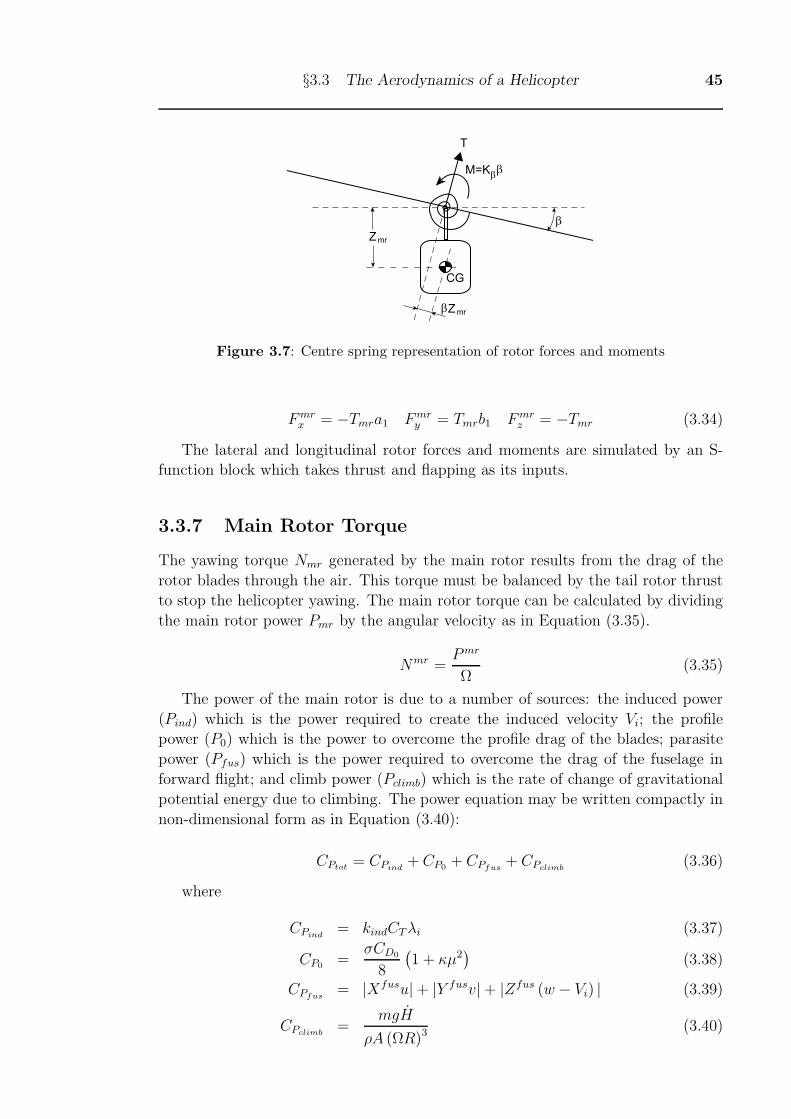
§3.3 The Aerodynamics of a Helicopter 45
β
T
CG
Z mr
βZ mr
M=K ββ
Figure 3.7: Centre spring representation of rotor forces and moments
Fmrx = −Tmra1 Fmr
y = Tmrb1 Fmrz = −Tmr (3.34)
The lateral and longitudinal rotor forces and moments are simulated by an S-
function block which takes thrust and flapping as its inputs.
3.3.7 Main Rotor Torque
The yawing torque Nmr generated by the main rotor results from the drag of the
rotor blades through the air. This torque must be balanced by the tail rotor thrust
to stop the helicopter yawing. The main rotor torque can be calculated by dividing
the main rotor power Pmr by the angular velocity as in Equation (3.35).
Nmr =Pmr
Ω(3.35)
The power of the main rotor is due to a number of sources: the induced power
(Pind) which is the power required to create the induced velocity Vi; the profile
power (P0) which is the power to overcome the profile drag of the blades; parasite
power (Pfus) which is the power required to overcome the drag of the fuselage in
forward flight; and climb power (Pclimb) which is the rate of change of gravitational
potential energy due to climbing. The power equation may be written compactly in
non-dimensional form as in Equation (3.40):
CPtot= CPind
+ CP0+ CPfus
+ CPclimb(3.36)
where
CPind= kindCTλi (3.37)
CP0=
σCD0
8
(1 + κμ2
)(3.38)
CPfus= |Xfusu| + |Y fusv| + |Zfus (w − Vi) | (3.39)
CPclimb=
mgH
ρA (ΩR)3 (3.40)
46 Helicopter Simulation and Control
The constant kind is a correction factor to compensate for tip losses and for the
inflow not being uniform. The constant κ compensates the profile drag power for
the effects of the reverse flow region and the spanwise flow over the rotor blade
in forward flight. Values of kind = 1.2 and κ = 4.7 have been assumed based on
suggestions by Leishman [163].
3.3.8 Tail Rotor
The calculation of tail rotor thrust is treated in the same way as the main rotor,
except the orientation is changed and flapping effects are not included. Another
S-function block was created to calculate the tail rotor thrust T tr and the tail rotor
power. The yawing moment from the tail rotor is calculated from the tail rotor
thrust using N tr = T trdtr where dtr is the distance from the centre of the tail rotor
to the centre of gravity.
3.3.9 Tailplane Forces and Moments
The Eagle helicopter is fitted with a vertical fin on the tailplane which helps to
stabilise the helicopter directionally in forward flight. The fin is treated like a wing
which creates lift when exposed to an angle of attack. The equations for the force
and moment contributions of the stabiliser are provided in Equation (3.44). The
drag force of the tailplane is lumped in with the drag force of the fuselage as a whole.
V vtR =
(u2 + w2
)(3.41)
αvt =v + rdvt
u(3.42)
F vty =
1
2ρV vt
R avtαvt (3.43)
Nvt = F vy d
vt (3.44)
3.3.10 Fuselage Forces
The fuselage drag forces are calculated along each body axis using the formulae in
Equation (3.47). The values Sx, Sy and Sz are the equivalent flat plate areas of the
fuselage in the respective directions.
F fusx =
ρ
2Sfusx u2 (3.45)
F fusY =
ρ
2Sfusy v2 (3.46)
F fusZ =
ρ
2Sfusz (w + Vi)
2 (3.47)

§3.3 The Aerodynamics of a Helicopter 47
3.3.11 Dynamics Subsystem
The helicopter dynamics are combined into a SIMULINKR© subsystem containing
all of the aerodynamic effects and rigid body dynamics as shown in Figure 3.8.
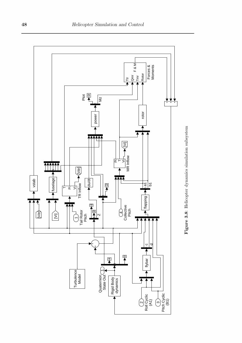
48 Helicopter Simulation and Control
Pto
t
1Q
uate
rnio
nS
tate
Out
T Pi
Vi
TR
Inflo
wT
urbu
lenc
eM
odel
vsta
b
flyba
rro
tor
flapp
ing
fuse
lage
pow
er
Pi T Vi
MR
Inflo
w
Rig
id B
ody
dyna
mic
s
[Vitr
]
[Vi]
[Vitr
]
[Vi]
Ttr
Qm
r
Tm
r
Rot
or
F &
M
For
ces
&M
omen
ts
du/d
t
emu
emu
emu
emu
emu
emu
emu
4C
olle
ctiv
eP
itch
3P
itch
Cyc
lic (
B1)2
Rol
l Cyc
lic(A
1)
1T
ail R
otor
Pitc
h
a1 b1
ZM
z
c d
Fig
ure
3.8
:H
elic
opte
rdynam
ics
sim
ula
tion
subsy
stem

§3.4 Servo Dynamics 49
The inputs to the subsystem are the collective pitch, tail rotor pitch and cyclic
pitch angles produced by the servos. The outputs are the state vector comprised of
position, local velocities, quaternion attitude, angular rates and accelerations. The
parameters used in the dynamics simulation are summarised in Appendix A.
3.4 Servo Dynamics
The Eagle helicopter has been fitted with DS8411 fast-response digital RC servos
manufactured by the Japan Radio Control Company (JR). Each servo contains an
integral PID controller that positions the servo in response to a Pulse Width Mod-
ulated control signal (PWM). The controller receives updates every 20 milliseconds
from the PWM stream. Various representations of RC servo dynamics have been
used ranging from first order to third order systems [157,173]. Gavrillets et al [157]
used a first order representation of the servo dynamics based on an identified band-
width for a typical RC servo of 6Hz, defined as being the frequency at which the
output lags the input with a 90 degree phase lag.
Brennan [174] conducted a detailed analysis of high-end digital servos and notes
that the frequency response of the servos is not in fact linear, being dependent on
amplitude. This agrees with observations made by driving a servo with sinewaves
ranging in frequency from 0.125Hz to 6.5Hz and measuring the servo horn position
with a sampled potentiometer output. My tests show that the magnitude response
begins to fall below unity at a speed of 1Hz for maximum deflection and 4Hz for
5 percent of full travel. At amplitudes below this, the servo Bode plot exhibits a
corner frequency of between 3.5Hz-4.0Hz. By comparing the frequency at which the
magnitude begins to drop, Ωcr, and the commanded amplitude θs, it is possible to
calculate the rate limit θmax using Equation (3.48) which is derived from consid-
ering when the derivative of the commanded sine wave exceeds the rate limit. At
amplitudes of 60◦, 48◦ and 36◦, the indicated rate limits were 314◦/sec, 301◦/sec
and 302◦/sec respectively. This agrees well with the 300◦/sec maximum angular
rate specification for the servo, provided by the manufacturer.
θmax = Ωcrθs (3.48)
Brennan achieved a good match to experimental data in his work by modeling
the servo as a second order dynamic with a rate limiter. Increased fidelity can be
achieved by including a small deadband of about 1 degree of servo horn travel that
is incorporated into COTS servos to reduce their power consumption. I have used
a similar approach to Brennan except I have used the simpler first order transfer
function Fs(s) in Equation (3.49) combined with a rate limiter of 300◦/sec, as the
measuring equipment was not accurate enough to determine the damping ratio of
the servo dynamics from the resonant peak and hence characterise the second or-
der dynamics properly. Noting that most other researchers use only a first order
representation this is not expected to be a significant source of error.
Fs(s) =1
1 + 0.05s(3.49)
50 Helicopter Simulation and Control
3.5 Atmospheric Disturbances
The aim of including turbulence into the simulation is to ensure that the sensing
and control system can cope with a real-world environment where wind effects can
be a significant challenge to station keeping. Only linear velocities are considered as
the small size of the helicopter means that gradient effects which might cause local
rotational flow are negligible [173]. The velocities corresponding to turbulence are
added to the body axis velocities provided by the rigid body dynamics block and
these velocities are fed as the freestream velocity input to the aerodynamic blocks.
The dominant techniques for simulating the effects of atmospheric turbulence
on flying vehicles are based on the Dryden and von Karman spectral models of
atmospheric turbulence. The Dryden spectra has been used for this simulation as it
can be most readily generated, simply by passing white noise through appropriate
linear filters [175]. The filters used to generate the Dryden spectra are described by
the transfer functions at Equations (3.50-3.51), reproduced from [176], where the
constant lengths Lu, Lv and Lw refer to the scale of turbulence. The output of the
velocities will be the relative wind velocities on all three axes. The parameter V
in the transfer functions is the relative speed of the aircraft to the airmass. The
equations are aimed at aircraft in forward flight where the longitudinal velocity is
dominant, hence the longitudinal filter is different to the lateral and vertical filters
which are the same. Whilst, in the case of a hovering helicopter, the wind can be
from any direction, for most work, the helicopter is flown with its nose into wind, so
that the speed V can be approximated by the mean wind speed. The scale lengths
can be found from a number of empirical sources such as ESDU [177] and MIL-F-
8785C [178]. The latter states that, at heights below 6m, which is representative of
the conditions that the experiments for this thesis were conducted, constant values
of Lu = Lv = 722.5m and Lw = 3m may be used. The turbulence intensity factors
σu, σv and σw depend on the mean speed of the relative wind and the altitude H .
They are described by Equations (3.52-3.53) which are reproduced from [178]. The
scale lengths and mean wind speed are entered in a graphical mask of the turbulence
block by the user before starting the simulation.
Fu(s) = σu
√2V
πLu
(1
s+ VLu
)(3.50)
Fv(s) = σv,w
√3V
πLv,w
⎛⎜⎝ s+ V√3Lv,w(
s+ VLv,w
)2
⎞⎟⎠ (3.51)
σw = 0.1umean (3.52)σuσw
=σvσw
=1
(0.177 + 0.000823H)0.4(3.53)
§3.6 Sensor Models 51
3.6 Sensor Models
The sensor block functions to simulate the characteristics of the sensors fitted to
the helicopter. The input to the block are the state variables from the helicopter
dynamics block comprising position, velocity, acceleration and atttitude. It consists
of the following subsytems:
• Inertial Measurement Unit. This block simulates the accelerometers, mag-
netometers and gyroscopes. A graphical mask allows offsets, gains and random
noise to be changed for each sensor. A two pole butterworth filter is imple-
mented for each sensor with the same corner frequencies as the actual sensors.
The accelerometers and gyroscopes have a 20Hz corner frequency with a 400Hz
sample rate whilst the magnetometers have a 10Hz corner frequency. All of
the inertial sensors are sampled at a 400Hz sample rate.
• Optic Flow. The optic flow sensor subsystem calculates the flow that would
be seen by a downwards looking camera. The inputs to the sensor are the
local velocities and the height above ground. Gaussian white noise is added
to the flows with the same variance as that measured from experiment.
• GPS. The position from the dynamics block is converted into global X, Y and
Z coordinates with an adjustable sample rate and added position white noise.
For the experiments in this thesis, a 20Hz sample rate was used to simulate
the NovAtel DGPS sensor fitted to the Eagle helicopter.
• Rangefinder. This block simulates a generic rangefinder for determining
height above ground such as a laser rangefinder or stereo camera. A graphical
mask allows sensor offset, scale error and random noise to be set.
• Beacon Position. This block generates a set of three azimuth and elevation
angles to simulated visual landmarks. The block simulates a camera sensor
with a 50 Hz frame rate and a single pixel quantisation. Angles are calculated
relative to the aircraft body axes.
3.7 State Estimator
To control a helicopter in hover, the following states are required: position, velocity,
attitude and rotation rates. These states must be deduced from the sensor outputs
using a state estimator. An S-function block was implemented to do this. The
block is capable of accepting input from a variety of different types of sensors. The
sensory inputs are grouped into inertial, GPS, optic flow, height and visual position
measurements. The outputs of the block are output with an update rate of 50Hz to
match the controller sample rate.
The estimator executes in a predict and correct cycle. The predict cycle occurs
at the sample rate of the incoming inertial data which is 400Hz. At each time
step the state equations are propagated based on the measured accelerations and
52 Helicopter Simulation and Control
rotation rates. The same equations used for the rigid body dynamics block are used
in the estimator with the exception of attitude which is propagated as two separate
reference vectors.
Position and velocity are corrected when measurements of these state variables
are taken. The GPS measurements arrive at 20Hz, the visual data arrive at the
speed of the frame grabber which is 50Hz and the height data arrive at the speed of
the sonar which is 25Hz. The corrections to each state x are made using Equation
(3.54) where k is an appropriate weighting factor and z is an observation of the
state. The correction term k for each sensor measurement is able to be modified by
the user by modifying the variables in the S-function GUI mask. The performance
of the estimator is generally not that sensitive to the values of k and these values
can be quickly set by trial and error to an appropriate value for the sensor noise
being simulated.
x∗ = x+ k (z − x) (3.54)
Attitude is stored and propagated inside the estimator as two vectors correspond-
ing to the gravity or downwards vector and a vector corresponding to the direction of
the local magnetic field. The gravity and magnetic field vectors are converted into a
rotation matrix and quaternion attitude representation as required. The vectors are
corrected at 50Hz using the measured magnetic vector from the magnetometers and
the gravitational vector measured by the accelerometers. It is assumed that over
a long time period, the accelerometer vector averages to that due to gravitational
acceleration. Hence the gravitational correction is based on the simple correction
cycle at Equation (3.54) with the observations being the measured accelerations.
During periods of rapid acceleration, this assumption causes errors in the pitch and
roll angles but I have found this does not upset the control of the helicopter in hover
or steady forward flight. For future work, it needs to be borne in mind that, if the
helicopter were to enter a banked turn, the attitude from the state estimator would
erect to a false horizon after a few seconds.
3.8 Simulation Validation
Initial adjustments of the simulation were made to match the trim control settings
of the simulation to the helicopter. The trim collective, aileron and elevator PWM
settings of the simulation were matched to values observed from flight test. The
simulation was validated against actual flight test data using frequency response
techniques. Time domain data were not used for validation since the helicopter is
dynamically unstable and requires constant attention by the pilot or control system
to keep in a stable hover. Due to small differences between the simulation and
plant, attempts to feed open loop control inputs recorded from flight test into the
simulation (or vice versa) result in rapid divergence from stable flight.
A chirp signal was used to stimulate the control inputs in both the simulation and
the actual plant (see Figure 3.9b), to generate a frequency response spectrum. The
chirp signal is made up of a sinusoidal signal of constant amplitude with a frequency
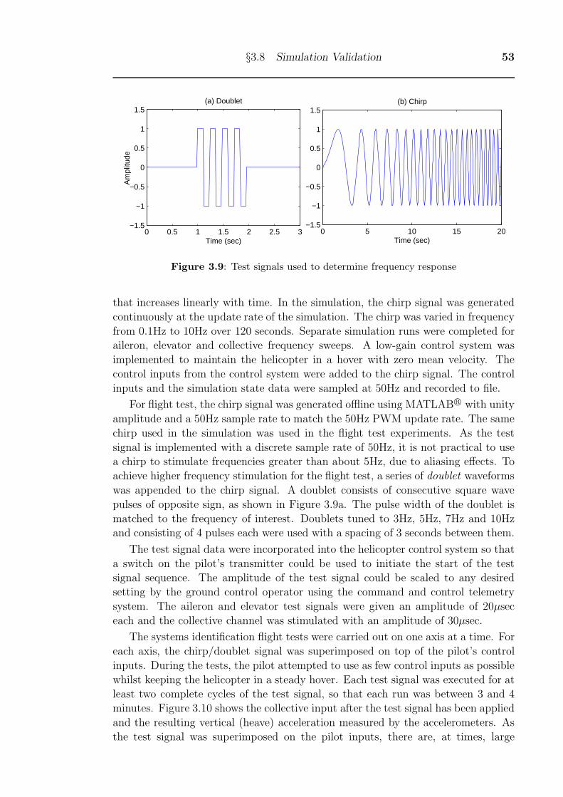
§3.8 Simulation Validation 53
0 0.5 1 1.5 2 2.5 3−1.5
−1
−0.5
0
0.5
1
1.5
Time (sec)
Am
plitu
de
(a) Doublet
0 5 10 15 20−1.5
−1
−0.5
0
0.5
1
1.5
Time (sec)
(b) Chirp
Figure 3.9: Test signals used to determine frequency response
that increases linearly with time. In the simulation, the chirp signal was generated
continuously at the update rate of the simulation. The chirp was varied in frequency
from 0.1Hz to 10Hz over 120 seconds. Separate simulation runs were completed for
aileron, elevator and collective frequency sweeps. A low-gain control system was
implemented to maintain the helicopter in a hover with zero mean velocity. The
control inputs from the control system were added to the chirp signal. The control
inputs and the simulation state data were sampled at 50Hz and recorded to file.
For flight test, the chirp signal was generated offline using MATLABR© with unity
amplitude and a 50Hz sample rate to match the 50Hz PWM update rate. The same
chirp used in the simulation was used in the flight test experiments. As the test
signal is implemented with a discrete sample rate of 50Hz, it is not practical to use
a chirp to stimulate frequencies greater than about 5Hz, due to aliasing effects. To
achieve higher frequency stimulation for the flight test, a series of doublet waveforms
was appended to the chirp signal. A doublet consists of consecutive square wave
pulses of opposite sign, as shown in Figure 3.9a. The pulse width of the doublet is
matched to the frequency of interest. Doublets tuned to 3Hz, 5Hz, 7Hz and 10Hz
and consisting of 4 pulses each were used with a spacing of 3 seconds between them.
The test signal data were incorporated into the helicopter control system so that
a switch on the pilot’s transmitter could be used to initiate the start of the test
signal sequence. The amplitude of the test signal could be scaled to any desired
setting by the ground control operator using the command and control telemetry
system. The aileron and elevator test signals were given an amplitude of 20μsec
each and the collective channel was stimulated with an amplitude of 30μsec.
The systems identification flight tests were carried out on one axis at a time. For
each axis, the chirp/doublet signal was superimposed on top of the pilot’s control
inputs. During the tests, the pilot attempted to use as few control inputs as possible
whilst keeping the helicopter in a steady hover. Each test signal was executed for at
least two complete cycles of the test signal, so that each run was between 3 and 4
minutes. Figure 3.10 shows the collective input after the test signal has been applied
and the resulting vertical (heave) acceleration measured by the accelerometers. As
the test signal was superimposed on the pilot inputs, there are, at times, large
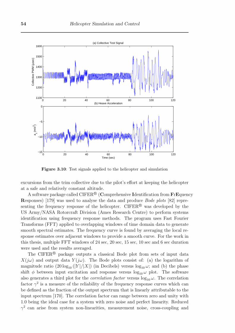
54 Helicopter Simulation and Control
0 20 40 60 80 100 1201100
1200
1300
1400
1500
1600
Col
lect
ive
PW
M (
μsec
)
(a) Collective Test Signal
0 20 40 60 80 100 120−15
−10
−5
0
Time (sec)
a z (m
/s2 )
(b) Heave Acceleration
Figure 3.10: Test signals applied to the helicopter and simulation
excursions from the trim collective due to the pilot’s effort at keeping the helicopter
at a safe and relatively constant altitude.
A software package called CIFERR© (Comprehensive Identification from FrEquency
Responses) [179] was used to analyse the data and produce Bode plots [82] repre-
senting the frequency response of the helicopter. CIFERR© was developed by the
US Army/NASA Rotorcraft Division (Ames Research Centre) to perform systems
identification using frequency response methods. The program uses Fast Fourier
Transforms (FFT) applied to overlapping windows of time domain data to generate
smooth spectral estimates. The frequency curve is found by averaging the local re-
sponse estimates over adjacent windows to provide a smooth curve. For the work in
this thesis, multiple FFT windows of 24 sec, 20 sec, 15 sec, 10 sec and 6 sec duration
were used and the results averaged.
The CIFER R© package outputs a classical Bode plot from sets of input data
X(jω) and output data Y (jω). The Bode plots consist of: (a) the logarithm of
magnitude ratio (20 log10 (|Y |/|X|) (in Decibels) versus log10 ω; and (b) the phase
shift φ between input excitation and response versus log10 ω plot. The software
also generates a third plot for the correlation factor versus log10 ω. The correlation
factor γ2 is a measure of the reliability of the frequency response curves which can
be defined as the fraction of the output spectrum that is linearly attributable to the
input spectrum [170]. The correlation factor can range between zero and unity with
1.0 being the ideal case for a system with zero noise and perfect linearity. Reduced
γ2 can arise from system non-linearities, measurement noise, cross-coupling and
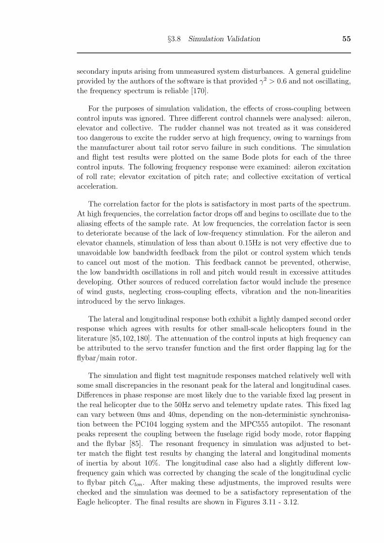
§3.8 Simulation Validation 55
secondary inputs arising from unmeasured system disturbances. A general guideline
provided by the authors of the software is that provided γ2 > 0.6 and not oscillating,
the frequency spectrum is reliable [170].
For the purposes of simulation validation, the effects of cross-coupling between
control inputs was ignored. Three different control channels were analysed: aileron,
elevator and collective. The rudder channel was not treated as it was considered
too dangerous to excite the rudder servo at high frequency, owing to warnings from
the manufacturer about tail rotor servo failure in such conditions. The simulation
and flight test results were plotted on the same Bode plots for each of the three
control inputs. The following frequency response were examined: aileron excitation
of roll rate; elevator excitation of pitch rate; and collective excitation of vertical
acceleration.
The correlation factor for the plots is satisfactory in most parts of the spectrum.
At high frequencies, the correlation factor drops off and begins to oscillate due to the
aliasing effects of the sample rate. At low frequencies, the correlation factor is seen
to deteriorate because of the lack of low-frequency stimulation. For the aileron and
elevator channels, stimulation of less than about 0.15Hz is not very effective due to
unavoidable low bandwidth feedback from the pilot or control system which tends
to cancel out most of the motion. This feedback cannot be prevented, otherwise,
the low bandwidth oscillations in roll and pitch would result in excessive attitudes
developing. Other sources of reduced correlation factor would include the presence
of wind gusts, neglecting cross-coupling effects, vibration and the non-linearities
introduced by the servo linkages.
The lateral and longitudinal response both exhibit a lightly damped second order
response which agrees with results for other small-scale helicopters found in the
literature [85,102,180]. The attenuation of the control inputs at high frequency can
be attributed to the servo transfer function and the first order flapping lag for the
flybar/main rotor.
The simulation and flight test magnitude responses matched relatively well with
some small discrepancies in the resonant peak for the lateral and longitudinal cases.
Differences in phase response are most likely due to the variable fixed lag present in
the real helicopter due to the 50Hz servo and telemetry update rates. This fixed lag
can vary between 0ms and 40ms, depending on the non-deterministic synchronisa-
tion between the PC104 logging system and the MPC555 autopilot. The resonant
peaks represent the coupling between the fuselage rigid body mode, rotor flapping
and the flybar [85]. The resonant frequency in simulation was adjusted to bet-
ter match the flight test results by changing the lateral and longitudinal moments
of inertia by about 10%. The longitudinal case also had a slightly different low-
frequency gain which was corrected by changing the scale of the longitudinal cyclic
to flybar pitch Clon. After making these adjustments, the improved results were
checked and the simulation was deemed to be a satisfactory representation of the
Eagle helicopter. The final results are shown in Figures 3.11 - 3.12.
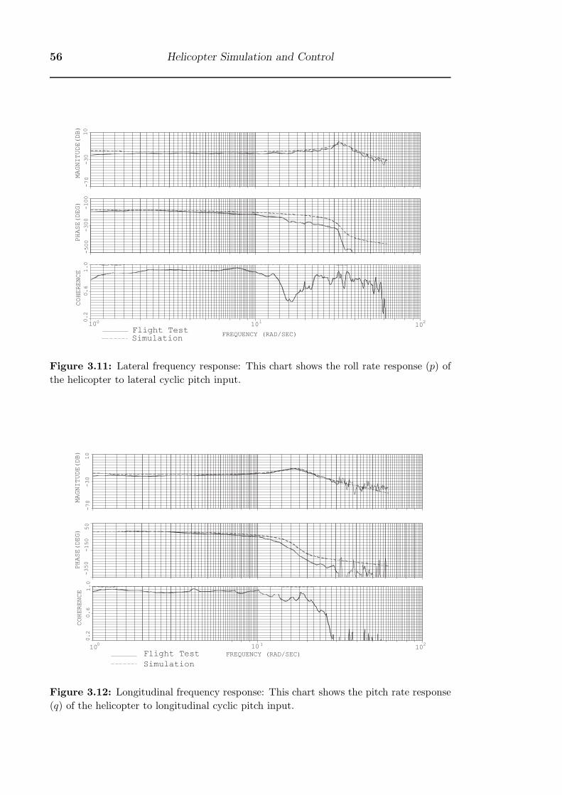
56 Helicopter Simulation and Control
Flight TestSimulation
MAGNITUDE(DB)
PHASE(DEG)
100 101
102
FREQUENCY (RAD/SEC)
COHERENCE
0.2
0.6
1.0
-500
-300
-100
-70
-30
10
Figure 3.11: Lateral frequency response: This chart shows the roll rate response (p) of
the helicopter to lateral cyclic pitch input.
Flight Test
Simulation
MAGNITUDE(DB)
PHASE(DEG)
FREQUENCY (RAD/SEC)
COHERENCE
0.2
0.6
1.0
-350
-150
50
-70
-30
10
10210 1
100
Figure 3.12: Longitudinal frequency response: This chart shows the pitch rate response
(q) of the helicopter to longitudinal cyclic pitch input.
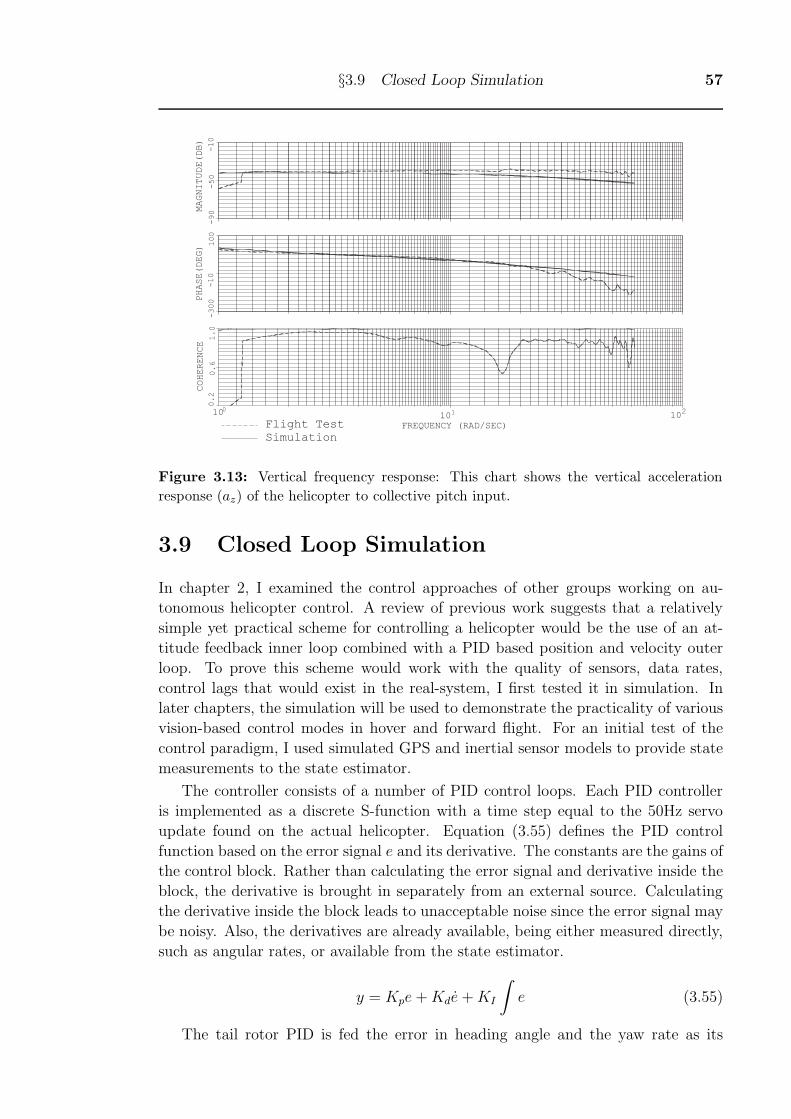
§3.9 Closed Loop Simulation 57
Simulation
Flight Test
MAGNITUDE(DB)
PHASE(DEG)
COHERENCE
0.2
0.6
1.0
-300
-10
-90
-50
100
-10
FREQUENCY (RAD/SEC)
102
101100
Figure 3.13: Vertical frequency response: This chart shows the vertical acceleration
response (az) of the helicopter to collective pitch input.
3.9 Closed Loop Simulation
In chapter 2, I examined the control approaches of other groups working on au-
tonomous helicopter control. A review of previous work suggests that a relatively
simple yet practical scheme for controlling a helicopter would be the use of an at-
titude feedback inner loop combined with a PID based position and velocity outer
loop. To prove this scheme would work with the quality of sensors, data rates,
control lags that would exist in the real-system, I first tested it in simulation. In
later chapters, the simulation will be used to demonstrate the practicality of various
vision-based control modes in hover and forward flight. For an initial test of the
control paradigm, I used simulated GPS and inertial sensor models to provide state
measurements to the state estimator.
The controller consists of a number of PID control loops. Each PID controller
is implemented as a discrete S-function with a time step equal to the 50Hz servo
update found on the actual helicopter. Equation (3.55) defines the PID control
function based on the error signal e and its derivative. The constants are the gains of
the control block. Rather than calculating the error signal and derivative inside the
block, the derivative is brought in separately from an external source. Calculating
the derivative inside the block leads to unacceptable noise since the error signal may
be noisy. Also, the derivatives are already available, being either measured directly,
such as angular rates, or available from the state estimator.
y = Kpe+Kde+KI
∫e (3.55)
The tail rotor PID is fed the error in heading angle and the yaw rate as its
58 Helicopter Simulation and Control
inputs. The inputs to the collective pitch PID are the error in altitude and the
vertical velocity. The lateral and longitudinal control scheme consists of an outer
and inner loop as proposed in Chapter 2.
The gains were tuned systematically using trial and error to converge on an
acceptable solution. In the first instance, the attitude control loop was tuned in-
dependently by turning off the outer loop and stopping the integration of velocity
and position in the dynamics block. Once satisfactory stability was demonstrated,
the outer loop was re-activated and the position and velocity gains were then tuned.
By disconnecting selected force and moment signals it was possible to tune pitch
and roll independently at first. Based on the approach of Ziegler and Nichols [80],
proportional gains on all loops were steadily increased to an ultimate gain Ku for
which the helicopter was marginally stable. The gains were then reduced to about
60% of Ku and then small adjustments were made to obtain a good compromise
between stability and speed of response.
Figure 3.14 shows the results of simulation of hover using the PID control scheme.
The desired reference position for the hover is X = 0m, Y = 0m, Z = 0m and
ψ = 0o. Turbulence corresponding to 5m/s mean wind speed is applied to the
relative air velocities. Sensor noise equivalent to that recorded from the actual
sensors is applied to the inertial and DGPS sensor blocks. The results show that
the helicopter is able to hold position and remains stable throughout the test. The
helicopter height wanders no more than 20cm from its datum position due to the
effect of the turbulence.
3.10 Summary
A closed-loop simulation of the Eagle helicopter has been developed using SIMULINKR©.
The model incorporates realistic sensor models, state estimation and control. In sim-
ulation, a position control loop scheme using PID control with an attitude feedback
inner loop has been shown to be a practical means of controlling the helicopter. The
simulation will be used in the following chapters to demonstrate the feasibility of
various sensing and control schemes.
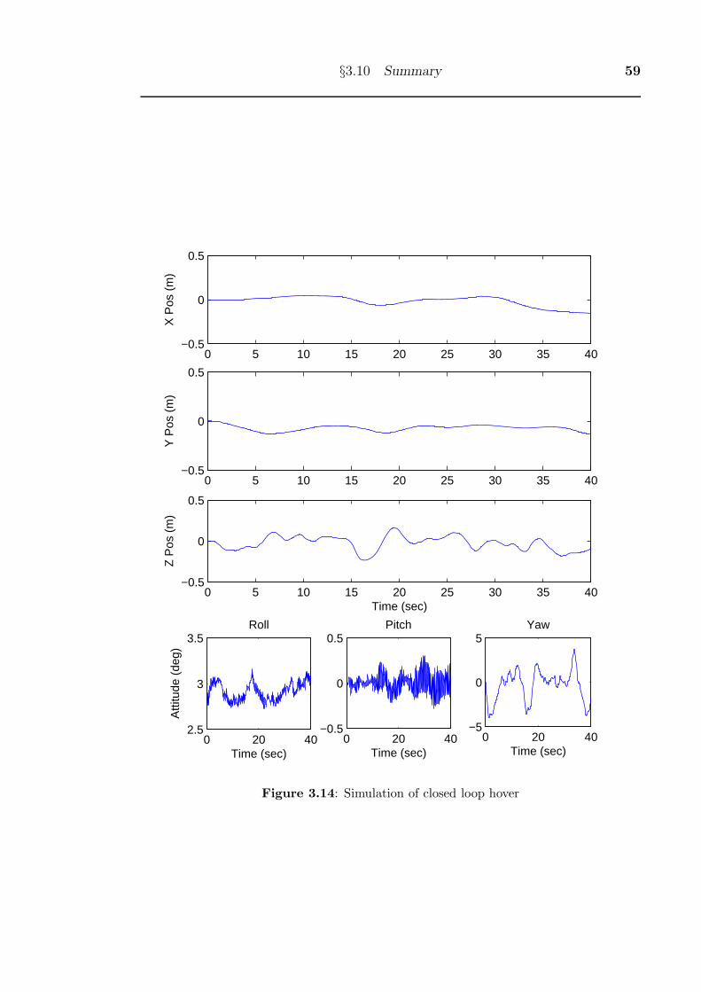
§3.10 Summary 59
0 5 10 15 20 25 30 35 40−0.5
0
0.5
X P
os (
m)
0 5 10 15 20 25 30 35 40−0.5
0
0.5
Y P
os (
m)
0 5 10 15 20 25 30 35 40−0.5
0
0.5
Z P
os (
m)
Time (sec)
0 20 402.5
3
3.5
Time (sec)
Atti
tude
(de
g)
Roll
0 20 40−0.5
0
0.5
Time (sec)
Pitch
0 20 40−5
0
5
Time (sec)
Yaw
Figure 3.14: Simulation of closed loop hover

Chapter 4
System Overview
4.1 Introduction
This chapter provides an overview of the platforms and systems used to conduct the
various flight experiments. This includes a discussion of the extensive embedded
systems development carried out by the author to field the avionics, telemetry and
sensors required to perform close loop flight experiments.
4.2 Helicopter Platforms
Experiments for this thesis were conducted on two separate helicopter types, both
comprising a conventional helicopter design with a single main rotor and a single
tail-rotor for anti-torque compensation. The first of these were built from kits man-
ufactured by the Japanese hobby company Hirobo. These kits are all based on
variants of the Eagle 60 size radio-controlled helicopter used by radio-control en-
thusiasts. The competition grade Eagles were selected on the basis of the perceived
quality of construction. Being of all carbon fibre construction, the airframe weight
is reduced, providing more capacity for avionics to be carried. Also, the Eagles
had all metal control linkages and high quality rotor parts, reducing concerns re-
lating to control slop and wear. In all, four Eagle helicopters were constructed and
instrumented for visual control research. A gasoline powered Eagle was also built
and tested but was abandoned due to low payload capability and high vibration.
Three of the helicopters were powered by internal combustion engines running on
methanol based fuel. A fourth helicopter was converted to electric power in 2005
using a brushless DC motor. This modification reduces vibration, eliminates fuel
spills on to avionics, eliminates problems with exhaust smoke obscuring the camera
and means that it is no longer necessary to account for fuel burnoff changing the
helicopter weight and balance in flight. I made a decision to transition all exper-
iments to the electric helicopter owing to these advantages. Unfortunately, it has
only been in the last two years that advances in battery technology have made an
electrical autonomous helicopter practical.
The second platform is an RMAX unmanned helicopter manufactured by Yamaha.
The RMAX helicopter used for this thesis is designated as a model L-50 by the
manufacturer and is designed for agricultural work. This RMAX has no inherent
autonomy other than a Yamaha Attitude Control System (YACS) which provides
61
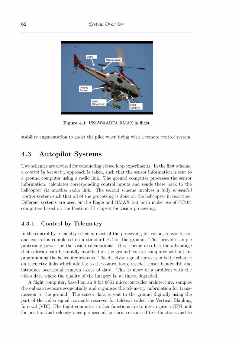
62 System Overview
Figure 4.1: UNSW@ADFA RMAX in flight
stability augmentation to assist the pilot when flying with a remote control system.
4.3 Autopilot Systems
Two schemes are devised for conducting closed loop experiments. In the first scheme,
a control by telemetry approach is taken, such that the sensor information is sent to
a ground computer using a radio link. The ground computer processes the sensor
information, calculates corresponding control inputs and sends these back to the
helicopter via another radio link. The second scheme involves a fully embedded
control system such that all of the processing is done on the helicopter in real-time.
Different systems are used on the Eagle and RMAX but both make use of PC104
computers based on the Pentium III chipset for vision processing.
4.3.1 Control by Telemetry
In the control by telemetry scheme, most of the processing for vision, sensor fusion
and control is completed on a standard PC on the ground. This provides ample
processing power for the vision calculations. This scheme also has the advantage
that software can be rapidly modified on the ground control computer without re-
programming the helicopter systems. The disadvantage of the system is the reliance
on telemetry links which add lag to the control loop, restrict sensor bandwidth and
introduce occasional random losses of data. This is more of a problem with the
video data where the quality of the imagery is, at times, degraded.
A flight computer, based on an 8 bit 8051 microcontroller architecture, samples
the onboard sensors sequentially and organises the telemetry information for trans-
mission to the ground. The sensor data is sent to the ground digitally using the
part of the video signal normally reserved for teletext called the Vertical Blanking
Interval (VBI). The flight computer’s other functions are to interrogate a GPS unit
for position and velocity once per second, perform sensor self-test functions and to
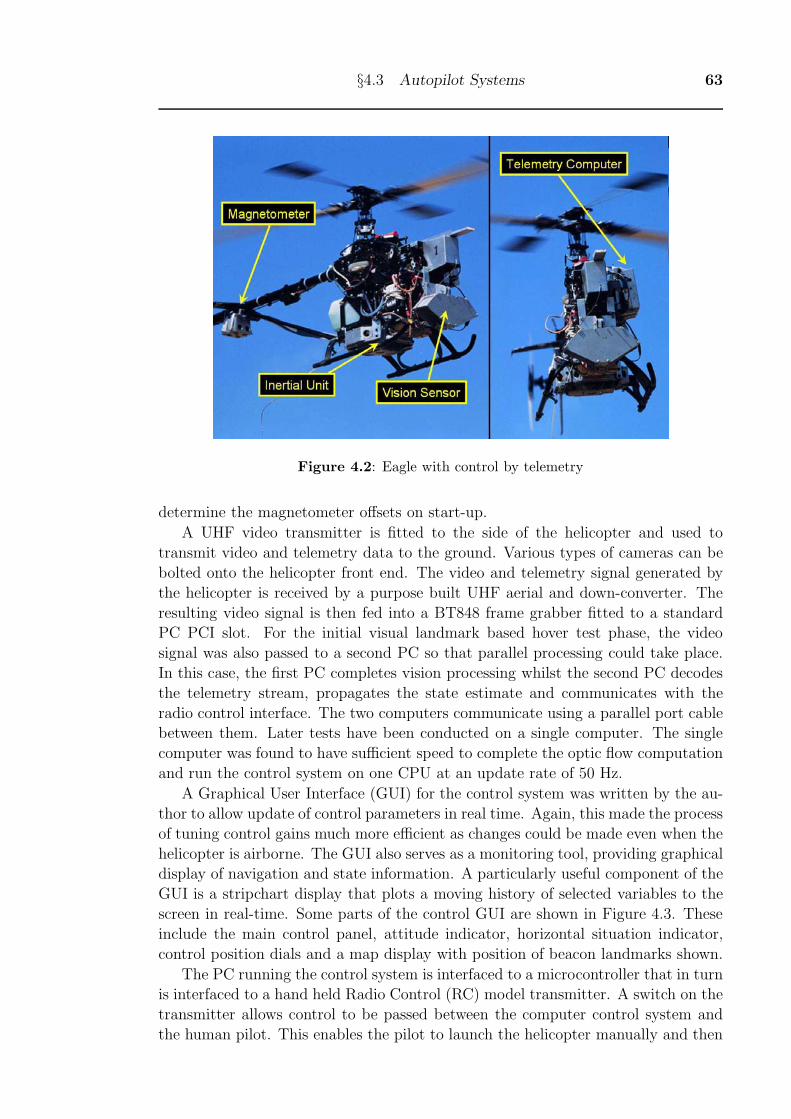
§4.3 Autopilot Systems 63
Figure 4.2: Eagle with control by telemetry
determine the magnetometer offsets on start-up.
A UHF video transmitter is fitted to the side of the helicopter and used to
transmit video and telemetry data to the ground. Various types of cameras can be
bolted onto the helicopter front end. The video and telemetry signal generated by
the helicopter is received by a purpose built UHF aerial and down-converter. The
resulting video signal is then fed into a BT848 frame grabber fitted to a standard
PC PCI slot. For the initial visual landmark based hover test phase, the video
signal was also passed to a second PC so that parallel processing could take place.
In this case, the first PC completes vision processing whilst the second PC decodes
the telemetry stream, propagates the state estimate and communicates with the
radio control interface. The two computers communicate using a parallel port cable
between them. Later tests have been conducted on a single computer. The single
computer was found to have sufficient speed to complete the optic flow computation
and run the control system on one CPU at an update rate of 50 Hz.
A Graphical User Interface (GUI) for the control system was written by the au-
thor to allow update of control parameters in real time. Again, this made the process
of tuning control gains much more efficient as changes could be made even when the
helicopter is airborne. The GUI also serves as a monitoring tool, providing graphical
display of navigation and state information. A particularly useful component of the
GUI is a stripchart display that plots a moving history of selected variables to the
screen in real-time. Some parts of the control GUI are shown in Figure 4.3. These
include the main control panel, attitude indicator, horizontal situation indicator,
control position dials and a map display with position of beacon landmarks shown.
The PC running the control system is interfaced to a microcontroller that in turn
is interfaced to a hand held Radio Control (RC) model transmitter. A switch on the
transmitter allows control to be passed between the computer control system and
the human pilot. This enables the pilot to launch the helicopter manually and then
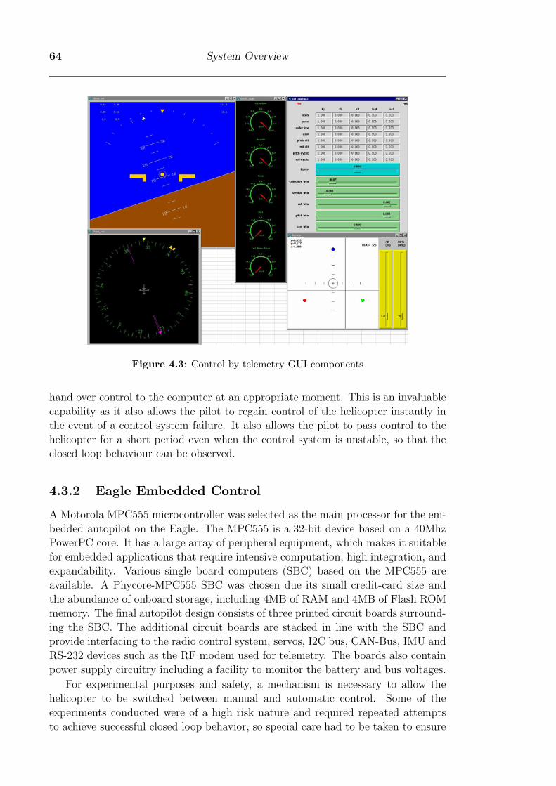
64 System Overview
Figure 4.3: Control by telemetry GUI components
hand over control to the computer at an appropriate moment. This is an invaluable
capability as it also allows the pilot to regain control of the helicopter instantly in
the event of a control system failure. It also allows the pilot to pass control to the
helicopter for a short period even when the control system is unstable, so that the
closed loop behaviour can be observed.
4.3.2 Eagle Embedded Control
A Motorola MPC555 microcontroller was selected as the main processor for the em-
bedded autopilot on the Eagle. The MPC555 is a 32-bit device based on a 40Mhz
PowerPC core. It has a large array of peripheral equipment, which makes it suitable
for embedded applications that require intensive computation, high integration, and
expandability. Various single board computers (SBC) based on the MPC555 are
available. A Phycore-MPC555 SBC was chosen due its small credit-card size and
the abundance of onboard storage, including 4MB of RAM and 4MB of Flash ROM
memory. The final autopilot design consists of three printed circuit boards surround-
ing the SBC. The additional circuit boards are stacked in line with the SBC and
provide interfacing to the radio control system, servos, I2C bus, CAN-Bus, IMU and
RS-232 devices such as the RF modem used for telemetry. The boards also contain
power supply circuitry including a facility to monitor the battery and bus voltages.
For experimental purposes and safety, a mechanism is necessary to allow the
helicopter to be switched between manual and automatic control. Some of the
experiments conducted were of a high risk nature and required repeated attempts
to achieve successful closed loop behavior, so special care had to be taken to ensure
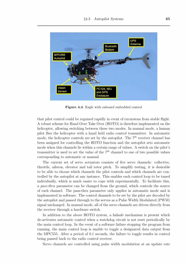
§4.3 Autopilot Systems 65
Figure 4.4: Eagle with onboard embedded control
that pilot control could be regained rapidly in event of excursions from stable flight.
A robust scheme for Hand Over Take Over (HOTO) is therefore implemented on the
helicopter, allowing switching between these two modes. In manual mode, a human
pilot flies the helicopter with a hand held radio control transmitter. In automatic
mode, the helicopter controls are set by the autopilot. The 7th receiver channel has
been assigned for controlling the HOTO function and the autopilot sets automatic
mode when this channels lie within a certain range of values. A switch on the pilot’s
transmitter is used to set the value of the 7th channel to one of two possible values
corresponding to automatic or manual.
The current set of servo actuators consists of five servo channels: collective,
throttle, aileron, elevator and tail rotor pitch. To simplify testing, it is desirable
to be able to choose which channels the pilot controls and which channels are con-
trolled by the autopilot at any instance. This enables each control loop to be tuned
individually, which is much easier to cope with experimentally. To facilitate this,
a pass-thru parameter can be changed from the ground, which controls the source
of each channel. The pass-thru parameter only applies in automatic mode and is
implemented in software. The control channels to be set by the pilot are decoded by
the autopilot and passed through to the servos as a Pulse Width Modulated (PWM)
signal unchanged. In manual mode, all of the servo channels are driven directly from
the receiver through a hardware switch.
In addition to the above HOTO system, a failsafe mechanism is present which
de-activates automatic control when a watchdog circuit is not reset periodically by
the main control loop. In the event of a software failure stopping the program from
running, the main control loop is unable to toggle a designated data output from
the MPC555. After a period of 0.1 seconds, the failure to toggle results in control
being passed back to the radio control receiver.
Servo channels are controlled using pulse width modulation at an update rate
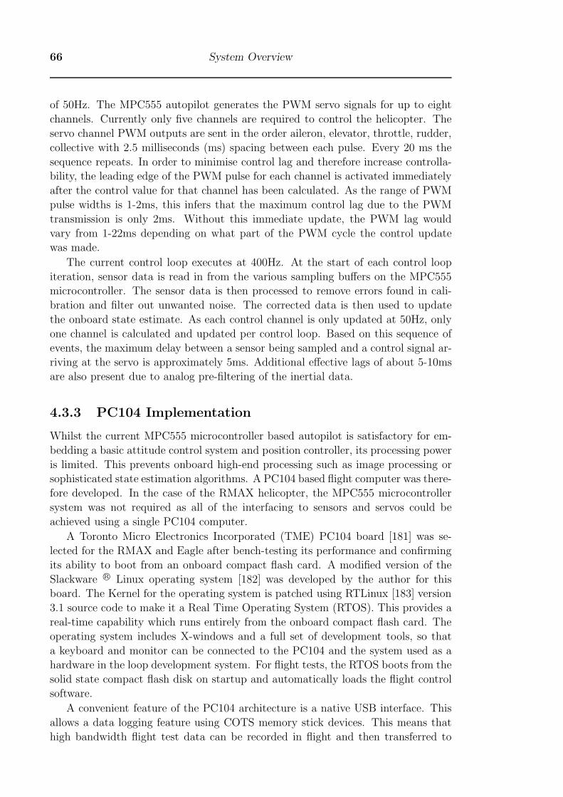
66 System Overview
of 50Hz. The MPC555 autopilot generates the PWM servo signals for up to eight
channels. Currently only five channels are required to control the helicopter. The
servo channel PWM outputs are sent in the order aileron, elevator, throttle, rudder,
collective with 2.5 milliseconds (ms) spacing between each pulse. Every 20 ms the
sequence repeats. In order to minimise control lag and therefore increase controlla-
bility, the leading edge of the PWM pulse for each channel is activated immediately
after the control value for that channel has been calculated. As the range of PWM
pulse widths is 1-2ms, this infers that the maximum control lag due to the PWM
transmission is only 2ms. Without this immediate update, the PWM lag would
vary from 1-22ms depending on what part of the PWM cycle the control update
was made.
The current control loop executes at 400Hz. At the start of each control loop
iteration, sensor data is read in from the various sampling buffers on the MPC555
microcontroller. The sensor data is then processed to remove errors found in cali-
bration and filter out unwanted noise. The corrected data is then used to update
the onboard state estimate. As each control channel is only updated at 50Hz, only
one channel is calculated and updated per control loop. Based on this sequence of
events, the maximum delay between a sensor being sampled and a control signal ar-
riving at the servo is approximately 5ms. Additional effective lags of about 5-10ms
are also present due to analog pre-filtering of the inertial data.
4.3.3 PC104 Implementation
Whilst the current MPC555 microcontroller based autopilot is satisfactory for em-
bedding a basic attitude control system and position controller, its processing power
is limited. This prevents onboard high-end processing such as image processing or
sophisticated state estimation algorithms. A PC104 based flight computer was there-
fore developed. In the case of the RMAX helicopter, the MPC555 microcontroller
system was not required as all of the interfacing to sensors and servos could be
achieved using a single PC104 computer.
A Toronto Micro Electronics Incorporated (TME) PC104 board [181] was se-
lected for the RMAX and Eagle after bench-testing its performance and confirming
its ability to boot from an onboard compact flash card. A modified version of the
Slackware R© Linux operating system [182] was developed by the author for this
board. The Kernel for the operating system is patched using RTLinux [183] version
3.1 source code to make it a Real Time Operating System (RTOS). This provides a
real-time capability which runs entirely from the onboard compact flash card. The
operating system includes X-windows and a full set of development tools, so that
a keyboard and monitor can be connected to the PC104 and the system used as a
hardware in the loop development system. For flight tests, the RTOS boots from the
solid state compact flash disk on startup and automatically loads the flight control
software.
A convenient feature of the PC104 architecture is a native USB interface. This
allows a data logging feature using COTS memory stick devices. This means that
high bandwidth flight test data can be recorded in flight and then transferred to
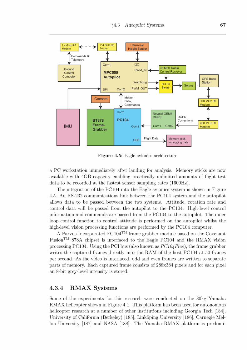
§4.3 Autopilot Systems 67
Com1
Com2
MPC555
Autopilot
DGPS
Corrections
Motion
Data,
Commands
Com1
Com2
PC104
USBFlight Data
Camera
BT878
Frame-
GrabberIMU
Commands &
Telemetry
2.4 GHz RF
Modem
Memory stick
for logging data
Novatel OEM4
DGPS
Com1 Com2
36 MHz Radio
Control Reciever
2.4 GHz RF
Modem
GPS Base
Station
900 MHz RF
Modem
900 MHz RF
Modem
Ground
Control
Computer
Servos
I2C
Ultrasonic
Height Sensor
PWM_IN
PWM_OUTSPI
WatchdogHOTO
Switch
Figure 4.5: Eagle avionics architecture
a PC workstation immediately after landing for analysis. Memory sticks are now
available with 4GB capacity enabling practically unlimited amounts of flight test
data to be recorded at the fastest sensor sampling rates (1600Hz).
The integration of the PC104 into the Eagle avionics system is shown in Figure
4.5. An RS-232 communications link between the PC104 system and the autopilot
allows data to be passed between the two systems. Attitude, rotation rate and
control data will be passed from the autopilot to the PC104. High-level control
information and commands are passed from the PC104 to the autopilot. The inner
loop control function to control attitude is performed on the autopilot whilst the
high-level vision processing functions are performed by the PC104 computer.
A Parvus Incorporated FG104TM frame grabber module based on the Coxenant
FusionTM 878A chipset is interfaced to the Eagle PC104 and the RMAX vision
processing PC104. Using the PCI bus (also known as PC104Plus), the frame grabber
writes the captured frames directly into the RAM of the host PC104 at 50 frames
per second. As the video is interlaced, odd and even frames are written to separate
parts of memory. Each captured frame consists of 288x384 pixels and for each pixel
an 8-bit grey-level intensity is stored.
4.3.4 RMAX Systems
Some of the experiments for this research were conducted on the 80kg Yamaha
RMAX helicopter shown in Figure 4.1. This platform has been used for autonomous
helicopter research at a number of other institutions including Georgia Tech [184],
University of California (Berkeley) [185], Linkoping University [186], Carnegie Mel-
lon University [187] and NASA [188]. The Yamaha RMAX platform is predomi-
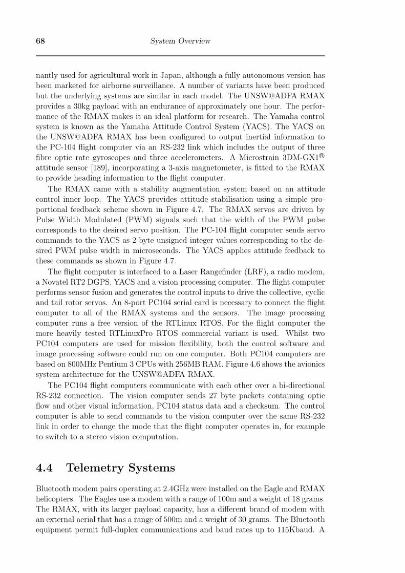
68 System Overview
nantly used for agricultural work in Japan, although a fully autonomous version has
been marketed for airborne surveillance. A number of variants have been produced
but the underlying systems are similar in each model. The UNSW@ADFA RMAX
provides a 30kg payload with an endurance of approximately one hour. The perfor-
mance of the RMAX makes it an ideal platform for research. The Yamaha control
system is known as the Yamaha Attitude Control System (YACS). The YACS on
the UNSW@ADFA RMAX has been configured to output inertial information to
the PC-104 flight computer via an RS-232 link which includes the output of three
fibre optic rate gyroscopes and three accelerometers. A Microstrain 3DM-GX1R©
attitude sensor [189], incorporating a 3-axis magnetometer, is fitted to the RMAX
to provide heading information to the flight computer.
The RMAX came with a stability augmentation system based on an attitude
control inner loop. The YACS provides attitude stabilisation using a simple pro-
portional feedback scheme shown in Figure 4.7. The RMAX servos are driven by
Pulse Width Modulated (PWM) signals such that the width of the PWM pulse
corresponds to the desired servo position. The PC-104 flight computer sends servo
commands to the YACS as 2 byte unsigned integer values corresponding to the de-
sired PWM pulse width in microseconds. The YACS applies attitude feedback to
these commands as shown in Figure 4.7.
The flight computer is interfaced to a Laser Rangefinder (LRF), a radio modem,
a Novatel RT2 DGPS, YACS and a vision processing computer. The flight computer
performs sensor fusion and generates the control inputs to drive the collective, cyclic
and tail rotor servos. An 8-port PC104 serial card is necessary to connect the flight
computer to all of the RMAX systems and the sensors. The image processing
computer runs a free version of the RTLinux RTOS. For the flight computer the
more heavily tested RTLinuxPro RTOS commercial variant is used. Whilst two
PC104 computers are used for mission flexibility, both the control software and
image processing software could run on one computer. Both PC104 computers are
based on 800MHz Pentium 3 CPUs with 256MB RAM. Figure 4.6 shows the avionics
system architecture for the UNSW@ADFA RMAX.
The PC104 flight computers communicate with each other over a bi-directional
RS-232 connection. The vision computer sends 27 byte packets containing optic
flow and other visual information, PC104 status data and a checksum. The control
computer is able to send commands to the vision computer over the same RS-232
link in order to change the mode that the flight computer operates in, for example
to switch to a stereo vision computation.
4.4 Telemetry Systems
Bluetooth modem pairs operating at 2.4GHz were installed on the Eagle and RMAX
helicopters. The Eagles use a modem with a range of 100m and a weight of 18 grams.
The RMAX, with its larger payload capacity, has a different brand of modem with
an external aerial that has a range of 500m and a weight of 30 grams. The Bluetooth
equipment permit full-duplex communications and baud rates up to 115Kbaud. A
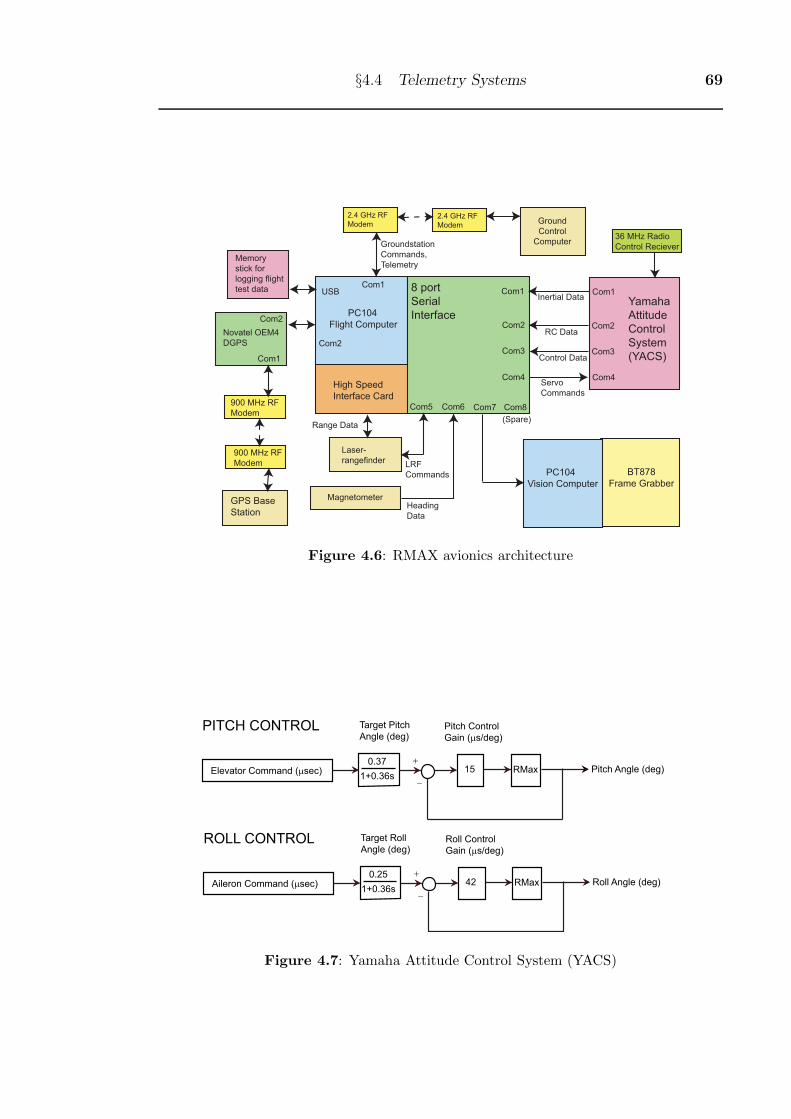
§4.4 Telemetry Systems 69
900 MHz RF
Modem
900 MHz RF
Modem
GPS Base
Station
36 MHz Radio
Control Reciever
Yamaha
Attitude
Control
System
(YACS)
8 port
Serial
Interface
Com1
Com2
Com3
Com4
Com5 Com6 Com7 Com8
Com1
Com2
Com3
Com4
Inertial Data
RC Data
Control Data
Servo
Commands
PC104
Flight Computer
Com1
Com2
USB
Memory
stick for
logging flight
test data
Novatel OEM4
DGPS
Com1
Com2
High Speed
Interface Card
(Spare)
Laser-
rangefinder LRF
Commands
MagnetometerHeading
Data
Groundstation
Commands,
Telemetry
2.4 GHz RF
Modem
2.4 GHz RF
Modem Ground
Control
Computer
Range Data
PC104
Vision Computer
BT878
Frame Grabber
Figure 4.6: RMAX avionics architecture
RMax150.37
1+0.36sElevator Command (μsec)
+
−
Pitch Angle (deg)
Pitch Control
Gain (μs/deg)
Target Pitch
Angle (deg)PITCH CONTROL
RMax420.25
1+0.36sAileron Command (μsec)
+
−
Roll Angle (deg)
Roll Control
Gain (μs/deg)
Target Roll
Angle (deg)ROLL CONTROL
Figure 4.7: Yamaha Attitude Control System (YACS)

70 System Overview
Figure 4.8: Eagle control GUI. Various parameters can be changed in flight. The page
shown in the diagram is used to adjust the controller gains remotely.
communications protocol was developed which intersperses 50Hz telemetry from the
helicopters with bi-directional command and control data between a ground station
and the helicopters. The protocol used by the Eagles and the RMAX is the same
except some platform specific packets apply to only one helicopter type.
The ground station comprises a personal computer running RTLinux with a serial
port connected to the Bluetooth modem. Both desktops and a laptop computer have
been used as the ground station for field work. The author has developed a real-time
communications stack for the ground station which encodes and decodes telemetry
packets between the helicopters and ground station. A GUI shown in figure 4.8 has
also been developed to allow the operator to easily interact with the communications
stack and send commands. This allows the type of telemetry being sent from the
helicopter to be changed by the press of a button. Graphical utilities have been
implemented to display all of the variables that can be sent from the helicopters.
Commands are sent to the helicopters in a set format depicted in Table 4.1. A
header character and checksum allows the helicopter to decode command packets of
variable length. The second character in the command data packet establishes the
length of the packet being received. Depending on the type of the command being
sent, the amount of command data being transmitted varies. Some commands such
as ‘start logging’ have no option data while some commands such as an instruction
to change a control gain may contain several bytes of option data. Every time a
command is sent, the command identifier field is incremented to define a unique
command. Upon successful receipt of a command packet, the autopilot sends an
acknowledgement packet containing the command identifier embedded in the orig-
inal message. The ground computer waits for a number of seconds after sending a
command to see if an acknowledgment has been sent by the autopilot. A record of
all commands sent to the helicopter is stored on the ground control computer. If
an acknowledgement is not received within a set time (usually about 5 seconds) for
§4.5 Sensors 71
Table 4.1: Telemetry packet structure
Byte Index Description0 Header character 0x551 Command character2 Length of packet in bytes (n)3 Command identifier MSB4 Command identifier LSB
5..n Data Optionsn+ 1 8 bit checksum
any of the commands sent, the command is resent. Fields within the control GUI
corresponding to transmitted commands are highlighted in a bright red colour until
an acknowledgement has been received. At present, 35 different types of command
packets have been implemented to perform tasks such as zeroing of sensors, changing
gains for PID controllers, changing flight modes and controlling logging of data.
Telemetry from the helicopters uses a similar scheme for transmitting sensor,
state and control data so that it may be displayed on the ground station GUI or
logged to a file. The type of telemetry being sent to the ground may be varied by
sending a command from the ground station.
4.5 Sensors
4.5.1 Vision Sensors
The RMAX and Eagle helicopter are fitted with a compatible camera mounting
bracket so that the cameras can be swapped between helicopters when required.
The mount allows the camera to be pointed to any tilt angle from straight down to
pointing forward along the helicopter longitudinal axis. For most of the experiments
discussed in this thesis, an analog Sony CCD image sensor is used. The camera
outputs a PAL standard composite video signal which is captured by the frame
grabber. The camera is housed in a 3cm x 3cm x 2.5cm enclosure with a lug to
attach to the mounting bracket on the nose of each helicopter.
4.5.2 Inertial Measurement Unit
Whilst the RMAX comes fitted with gyroscopes and accelerometers, the Eagle heli-
copters had to be fitted with inertial sensors. When the project commenced, funding
was not available for a satisfactory COTS Inertial Measurement Unit (IMU), forcing
the construction of an in-house system. Three different IMU designs have been con-
structed, calibrated and test flown on the Eagle helicopters during the evolution of
this project. The first of these comprises a sensor cluster with three accelerometers
and three Murata ENV-05D gyroscopes in the same case. A separate box with a
three-axis magnetometer system is used in conjunction with this system to provide
72 System Overview
all the sensors needed for a complete Attitude Heading Reference System (AHRS).
A 16bit Analog to Digital Converter (ADC) is installed in each box and interfaced
to a remote microcontroller.
The other two IMU designs comprise three accelerometers, three magnetometers
and three rate gyroscopes with ADC circuity and an integrated microcontroller in
the same housing. The primary difference between these two IMUs is that the latest
device uses smaller Analog Devices ADXRS-150ABG [190] gyroscopes rather than
the Murata gyroscopes.
The axes of each set of sensors are arranged in an orthogonal fashion so that
the orientation and motion of the helicopter along all three axes can be determined.
The sensors rotate with the body axes system of the helicopter, which is fixed to the
aircraft centre of gravity and rotates as the aircraft’s attitude changes. The faces of
the metal IMU case are deliberately machined to be square to within 0.1 degrees.
The IMU x,y and z reference axes are defined in a direction normal to the faces of
the IMU case. The naming of the IMU x,y and z reference axes were selected so
that when the IMU is installed in the helicopter, the axes would then be coincident
with the helicopter body axes. The sensors used in the Inertial Measurement Units
are as follows:
a. Accelerometers. The accelerometers measure the sum of gravitational accel-
eration and the velocity derivatives of the IMU. If the assumption is made that the
motion derivatives average out to zero over a long enough time period, then the
mean values of the accelerometers can be assumed to represent the gravity vector.
As the axes of the accelerometers are aligned with the helicopter axes, the gravity
vector is measured relative to the helicopter. In effect, the accelerometers act like
a pendulum hanging from beneath the helicopter. Such a pendulum would tend to
hang vertically downwards but would swing from side to side in response to hori-
zontal accelerations. As well as providing a noisy estimate of the vertical direction,
the accelerometers provide motion derivatives, which can be integrated to provide
velocity.
b. Magnetometers. Each magnetometer provides a voltage output in proportion
to the degree of alignment with the local magnetic field. Using three orthogonal
magnetometers it is possible to measure the relative orientation of the earth’s mag-
netic vector to the helicopter. The horizontal component of the earth’s magnetic
field points towards the magnetic North pole. When combined with the gravity vec-
tor measured by the accelerometers, the helicopter is able to determine its complete
orientation including pitch, roll and yaw.
c. Gyroscopes. Three piezoelectric gyroscopes provide a voltage output propor-
tional to measured rotation rate around the aircraft body axes. By integrating the
gyroscopic rates, the attitude of the helicopter can be updated. The Murata gyro-
scopes used have a range of−90◦/sec to +90◦/sec and the Analog Devices gyroscopes
have a range of −150◦/sec to +150◦/sec.In designing the IMUs for the MPC555 autopilot, the aim is to achieve the
highest sampling rate possible without interrupting the processor continuously. This
is achieved by having a separate processor to carry out the low-level sampling,
leaving the MPC555 to run the state estimation algorithm without interruption.
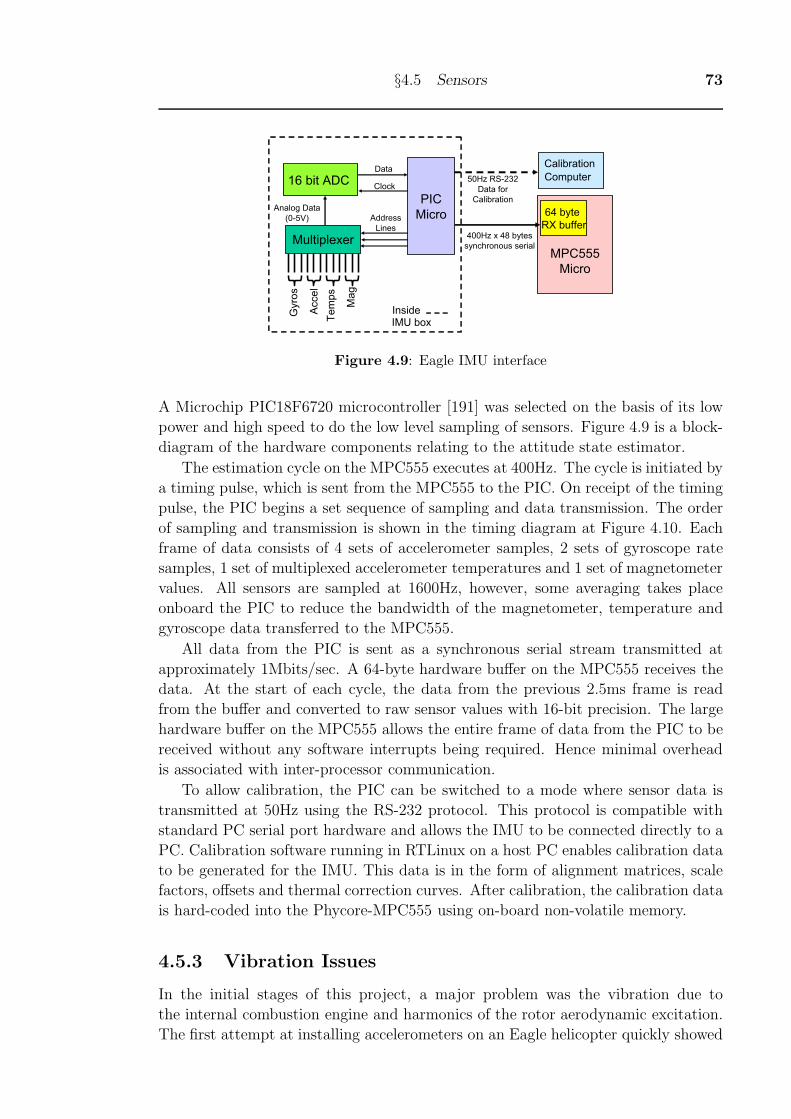
§4.5 Sensors 73
16 bit ADC
Multiplexer
Gyro
s
Acce
l
Tem
ps
Ma
g
Analog Data
(0-5V) Address
Lines
PIC
Micro
50Hz RS-232
Data for
Calibration
MPC555
Micro
64 byte
RX buffer400Hz x 48 bytes
synchronous serial
Calibration
Computer
Inside IMU box
Clock
Data
Figure 4.9: Eagle IMU interface
A Microchip PIC18F6720 microcontroller [191] was selected on the basis of its low
power and high speed to do the low level sampling of sensors. Figure 4.9 is a block-
diagram of the hardware components relating to the attitude state estimator.
The estimation cycle on the MPC555 executes at 400Hz. The cycle is initiated by
a timing pulse, which is sent from the MPC555 to the PIC. On receipt of the timing
pulse, the PIC begins a set sequence of sampling and data transmission. The order
of sampling and transmission is shown in the timing diagram at Figure 4.10. Each
frame of data consists of 4 sets of accelerometer samples, 2 sets of gyroscope rate
samples, 1 set of multiplexed accelerometer temperatures and 1 set of magnetometer
values. All sensors are sampled at 1600Hz, however, some averaging takes place
onboard the PIC to reduce the bandwidth of the magnetometer, temperature and
gyroscope data transferred to the MPC555.
All data from the PIC is sent as a synchronous serial stream transmitted at
approximately 1Mbits/sec. A 64-byte hardware buffer on the MPC555 receives the
data. At the start of each cycle, the data from the previous 2.5ms frame is read
from the buffer and converted to raw sensor values with 16-bit precision. The large
hardware buffer on the MPC555 allows the entire frame of data from the PIC to be
received without any software interrupts being required. Hence minimal overhead
is associated with inter-processor communication.
To allow calibration, the PIC can be switched to a mode where sensor data is
transmitted at 50Hz using the RS-232 protocol. This protocol is compatible with
standard PC serial port hardware and allows the IMU to be connected directly to a
PC. Calibration software running in RTLinux on a host PC enables calibration data
to be generated for the IMU. This data is in the form of alignment matrices, scale
factors, offsets and thermal correction curves. After calibration, the calibration data
is hard-coded into the Phycore-MPC555 using on-board non-volatile memory.
4.5.3 Vibration Issues
In the initial stages of this project, a major problem was the vibration due to
the internal combustion engine and harmonics of the rotor aerodynamic excitation.
The first attempt at installing accelerometers on an Eagle helicopter quickly showed
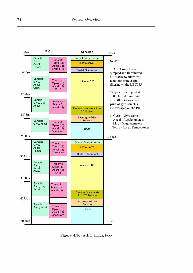
74 System Overview
Correct Sensor errors
Update servo 1
Digital Filter Accel
Attitude EKF
Process commands from RF Modem
Interrogate Misc Sensors
Spare
Sample: Gyro, Accel, Temps
Sample: Gyro, Accel, Ch16
Sample :Gyro, Mag, Accel
Sample: Gyro, Accel
Temp (x3) Accel (x3) Frame No
Sample: Gyro, Accel, Temps
Sample: Gyro, Accel, Ch16
Sample: Gyro, Mag, Accel
Sample: Gyro, Accel
5 ms
2.5 ms
0 ms 0μs
1875μs
625μs
1250μs
2500μs
3125μs
3750μs
4375μs
5000μs
PIC MPC555
Gyros (x3) Accel (x3)
Ch16
Mag x 3, Accel (x3)
Gyros (x3) Accel (x3) Checksum
Temp (x3) Accel (x3) Frame No
Gyros (x3) Accel (x3)
Ch16
Mags x 3 Accel (x3)
Gyros (x3) Accel (x3) Checksum
Correct Sensor errors
Update Servo 2
Digital Filter Accel
Attitude EKF
Process Commands from RF Modem
Interrogate Misc Sensors
Spare
Transmit:
Transmit:
Transmit:
Transmit:
Transmit:
Transmit:
Transmit:
Transmit:
NOTES:
1. Accelerometers are
sampled and transmitted
at 1600Hz to allow for
more elaborate digital
filtering on the MPC555.
2.Gyros are sampled at
1600Hz and transmitted
at 800Hz. Consecutive
pairs of gyro samples
are averaged on the PIC.
3. Gyros - Gyroscopes
Accel - Accelerometers
Mag - Magnetometers
Temp - Accel. Temperatures
Figure 4.10: AHRS timing loop
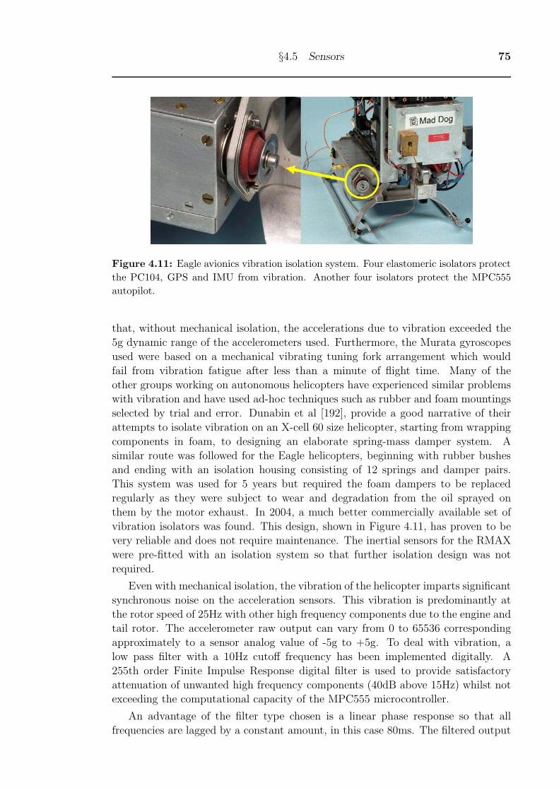
§4.5 Sensors 75
Figure 4.11: Eagle avionics vibration isolation system. Four elastomeric isolators protect
the PC104, GPS and IMU from vibration. Another four isolators protect the MPC555
autopilot.
that, without mechanical isolation, the accelerations due to vibration exceeded the
5g dynamic range of the accelerometers used. Furthermore, the Murata gyroscopes
used were based on a mechanical vibrating tuning fork arrangement which would
fail from vibration fatigue after less than a minute of flight time. Many of the
other groups working on autonomous helicopters have experienced similar problems
with vibration and have used ad-hoc techniques such as rubber and foam mountings
selected by trial and error. Dunabin et al [192], provide a good narrative of their
attempts to isolate vibration on an X-cell 60 size helicopter, starting from wrapping
components in foam, to designing an elaborate spring-mass damper system. A
similar route was followed for the Eagle helicopters, beginning with rubber bushes
and ending with an isolation housing consisting of 12 springs and damper pairs.
This system was used for 5 years but required the foam dampers to be replaced
regularly as they were subject to wear and degradation from the oil sprayed on
them by the motor exhaust. In 2004, a much better commercially available set of
vibration isolators was found. This design, shown in Figure 4.11, has proven to be
very reliable and does not require maintenance. The inertial sensors for the RMAX
were pre-fitted with an isolation system so that further isolation design was not
required.
Even with mechanical isolation, the vibration of the helicopter imparts significant
synchronous noise on the acceleration sensors. This vibration is predominantly at
the rotor speed of 25Hz with other high frequency components due to the engine and
tail rotor. The accelerometer raw output can vary from 0 to 65536 corresponding
approximately to a sensor analog value of -5g to +5g. To deal with vibration, a
low pass filter with a 10Hz cutoff frequency has been implemented digitally. A
255th order Finite Impulse Response digital filter is used to provide satisfactory
attenuation of unwanted high frequency components (40dB above 15Hz) whilst not
exceeding the computational capacity of the MPC555 microcontroller.
An advantage of the filter type chosen is a linear phase response so that all
frequencies are lagged by a constant amount, in this case 80ms. The filtered output
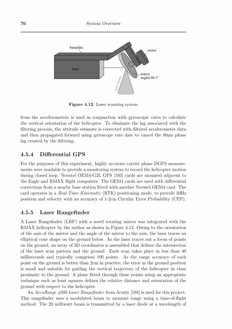
76 System Overview
Figure 4.12: Laser scanning system
from the accelerometers is used in conjunction with gyroscopic rates to calculate
the vertical orientation of the helicopter. To eliminate the lag associated with the
filtering process, the attitude estimate is corrected with filtered accelerometer data
and then propagated forward using gyroscope rate date to cancel the 80ms phase
lag created by the filtering.
4.5.4 Differential GPS
For the purposes of this experiment, highly accurate carrier phase DGPS measure-
ments were available to provide a monitoring system to record the helicopter motion
during closed loop. Novatel OEM4-G2L GPS [193] cards are mounted adjacent to
the Eagle and RMAX flight computers. The OEM4 cards are used with differential
corrections from a nearby base station fitted with another Novatel OEM4 card. The
card operates in a Real-Time Kinematic (RTK) positioning mode, to provide 20Hz
position and velocity with an accuracy of 1-2cm Circular Error Probability (CEP).
4.5.5 Laser Rangefinder
A Laser Rangefinder (LRF) with a novel rotating mirror was integrated with the
RMAX helicopter by the author as shown in Figure 4.12. Owing to the orientation
of the axis of the mirror and the angle of the mirror to the axis, the laser traces an
elliptical cone shape on the ground below. As the laser traces out a locus of points
on the ground, an array of 3D coordinates is assembled that defines the intersection
of the laser scan pattern and the ground. Each scan takes place in less than 40
milliseconds and typically comprises 100 points. As the range accuracy of each
point on the ground is better than 2cm in practice, the error in the ground position
is small and suitable for guiding the vertical trajectory of the helicopter in close
proximity to the ground. A plane fitted through these points using an appropriate
technique such as least squares defines the relative distance and orientation of the
ground with respect to the helicopter.
An AccuRange 4000 Laser Rangefinder from Acuity [194] is used for this project.
This rangefinder uses a modulated beam to measure range using a time-of-flight
method. The 20 milliwatt beam is transmitted by a laser diode at a wavelength of

§4.5 Sensors 77
Figure 4.13: Rotating mirror assembly
780nm. The manufacturer claims a stated range of a few cm up to 16.5m with an
accuracy of 2.5mm. Although Acuity provide a linecaster system of their own, this
system is replaced to obtain the conical scan pattern peculiar to this application. A
mirror is machined out of a block of aluminium with a reflecting face cut at 86.5◦ to
the axis of the motor. This provides a distorted cone with an average included angle
of approximately 7.0◦ as the mirror spins. The mirror is hand polished and then
electroplated with gold to provide a reflectivity to the laser light of 95%. Figure
4.13 shows the mirror assembled on the drive motor.
To obtain a sufficiently fast scan rate, the mirror is spun at least 1500RPM or 25
cycles per second. As the mirror is not symmetrical about the axis, the imbalance of
the mirror needed to be addressed to operate at these speeds. A balancing collar was
therefore designed out of stainless steel to offset the static and dynamic imbalance
of the mirror. The collar is of constant thickness but the end profile is machined to
maintain the centre of gravity of each longitudinal slice of the combined collar/mirror
assembly on the axis of the shaft. Once assembled, the balance of the assembly is
finely adjusted by adding tiny weights and removing material where required. The
entire assembly with LRF and mirror is mounted under the belly of the RMAX
using 4 cable mounts for vibration isolation. The mounts were tuned to attenuate
vibrations at the main rotor frequency and above.
The mirror is mounted directly onto the shaft of a small DC motor, which is itself
mounted at 45◦ to the beam of the laser rangefinder. The speed of the motor can
be adjusted by changing the input voltage using a multi-position switch. An optical
encoder is fitted on the shaft of the motor. The encoder outputs a quadrature pulse
train with a precision of 4096 pulses per revolution. An index pulse is triggered
once per revolution for synchronisation purposes. The pulse train from the encoder
is monitored by an analogue safety interlock system that automatically disrupts
power to the laser in case of the mirror speed falling below 1000rpm. This stops the
laser from being concentrated on to a single spot for too long and causing a hazard
to observers.
The rangefinder and encoder signals are read into a PC104 form factor High
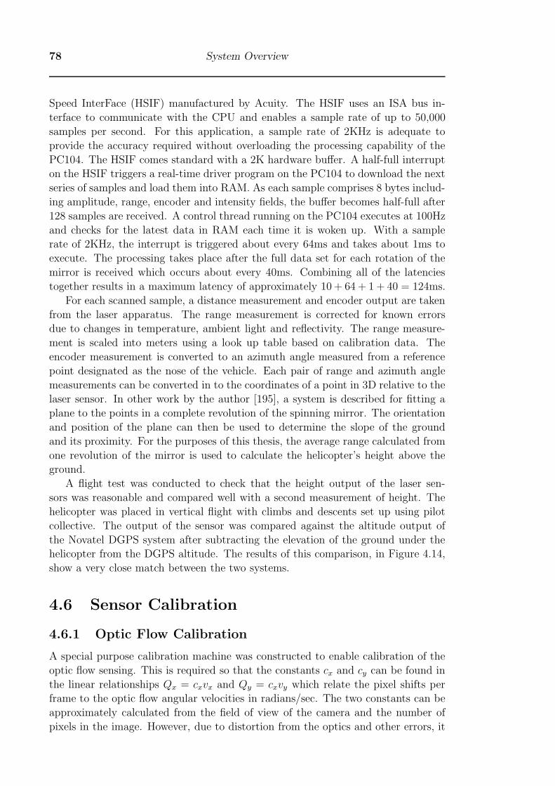
78 System Overview
Speed InterFace (HSIF) manufactured by Acuity. The HSIF uses an ISA bus in-
terface to communicate with the CPU and enables a sample rate of up to 50,000
samples per second. For this application, a sample rate of 2KHz is adequate to
provide the accuracy required without overloading the processing capability of the
PC104. The HSIF comes standard with a 2K hardware buffer. A half-full interrupt
on the HSIF triggers a real-time driver program on the PC104 to download the next
series of samples and load them into RAM. As each sample comprises 8 bytes includ-
ing amplitude, range, encoder and intensity fields, the buffer becomes half-full after
128 samples are received. A control thread running on the PC104 executes at 100Hz
and checks for the latest data in RAM each time it is woken up. With a sample
rate of 2KHz, the interrupt is triggered about every 64ms and takes about 1ms to
execute. The processing takes place after the full data set for each rotation of the
mirror is received which occurs about every 40ms. Combining all of the latencies
together results in a maximum latency of approximately 10 + 64 + 1 + 40 = 124ms.
For each scanned sample, a distance measurement and encoder output are taken
from the laser apparatus. The range measurement is corrected for known errors
due to changes in temperature, ambient light and reflectivity. The range measure-
ment is scaled into meters using a look up table based on calibration data. The
encoder measurement is converted to an azimuth angle measured from a reference
point designated as the nose of the vehicle. Each pair of range and azimuth angle
measurements can be converted in to the coordinates of a point in 3D relative to the
laser sensor. In other work by the author [195], a system is described for fitting a
plane to the points in a complete revolution of the spinning mirror. The orientation
and position of the plane can then be used to determine the slope of the ground
and its proximity. For the purposes of this thesis, the average range calculated from
one revolution of the mirror is used to calculate the helicopter’s height above the
ground.
A flight test was conducted to check that the height output of the laser sen-
sors was reasonable and compared well with a second measurement of height. The
helicopter was placed in vertical flight with climbs and descents set up using pilot
collective. The output of the sensor was compared against the altitude output of
the Novatel DGPS system after subtracting the elevation of the ground under the
helicopter from the DGPS altitude. The results of this comparison, in Figure 4.14,
show a very close match between the two systems.
4.6 Sensor Calibration
4.6.1 Optic Flow Calibration
A special purpose calibration machine was constructed to enable calibration of the
optic flow sensing. This is required so that the constants cx and cy can be found in
the linear relationships Qx = cxvx and Qy = cxvy which relate the pixel shifts per
frame to the optic flow angular velocities in radians/sec. The two constants can be
approximately calculated from the field of view of the camera and the number of
pixels in the image. However, due to distortion from the optics and other errors, it
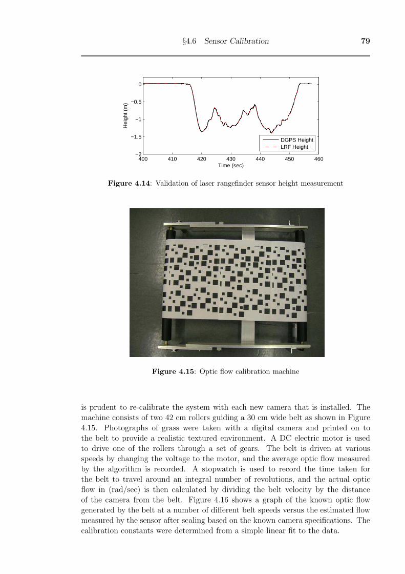
§4.6 Sensor Calibration 79
400 410 420 430 440 450 460−2
−1.5
−1
−0.5
0
Time (sec)
Hei
ght (
m)
DGPS HeightLRF Height
Figure 4.14: Validation of laser rangefinder sensor height measurement
Figure 4.15: Optic flow calibration machine
is prudent to re-calibrate the system with each new camera that is installed. The
machine consists of two 42 cm rollers guiding a 30 cm wide belt as shown in Figure
4.15. Photographs of grass were taken with a digital camera and printed on to
the belt to provide a realistic textured environment. A DC electric motor is used
to drive one of the rollers through a set of gears. The belt is driven at various
speeds by changing the voltage to the motor, and the average optic flow measured
by the algorithm is recorded. A stopwatch is used to record the time taken for
the belt to travel around an integral number of revolutions, and the actual optic
flow in (rad/sec) is then calculated by dividing the belt velocity by the distance
of the camera from the belt. Figure 4.16 shows a graph of the known optic flow
generated by the belt at a number of different belt speeds versus the estimated flow
measured by the sensor after scaling based on the known camera specifications. The
calibration constants were determined from a simple linear fit to the data.

80 System Overview
0
20
40
60
80
100
120
140
160
180
0 20 40 60 80 100 120 140 160
Measured Flow (rad/sec)
Actu
al
Flo
w (
rad
/sec)
Figure 4.16: Calibration of optic flow scale
4.6.2 IMU Calibration
One of the major problems facing attitude estimators is the effect of sensor error.
Various forms of sensor errors exist including misalignment, offset, gain and thermal
drift. With careful calibration, many of the fixed errors can be reduced significantly.
Specifically, calibration procedures have been devised for the following errors:
a. Sensor misalignment. The alignment of the axis of each sensor within its
package is generally only known to within a few degrees. Consequently, it is nec-
essary to determine the actual alignment of the sensors with respect to the IMU
housing. Misalignment of the sensors results in cross-coupling between the various
sensor axes. Misalignment is corrected by multiplying the sensor values by a 3x3
alignment matrix. This alignment matrix is determined in a set of separate calibra-
tion processes devised for each of the accelerometer, gyroscope and magnetometer
sensors.
b. Gain. Each sensor outputs a voltage between 0 and 5V which is proportional
to the variable being measured. The sensors have a linear relationship between input
and output and the gain of each sensor refers to the slope of the voltage versus input
variable. The gain is slightly different for each sensor and is determined during
calibration.
c. Offset. Each sensor has a nominal output of about 2.5v when the measured
variable is zero. For accelerometers and gyroscope, this applies to the case where
there is no acceleration or no rotation respectively. For the magnetometers, a zero
reading occurs when the magnetic field is perpendicular to the sensor. The null
position of each sensor is usually slightly offset from 2.5v due to variations during
the manufacturing process. This offset is measured during calibration and stored
for each sensor in non-volatile memory on the MPC555 autopilot.
d. Thermal Drift. Variations in temperature cause a shift in the offset of each
sensor. This shift can be measured during calibration by cycling the temperature of
§4.7 Attitude Determination 81
the IMU in a thermally controlled environment and measuring the change in sensor
reading. As the thermal drift is the only error that changes dynamically, it is the
only error that needs to be accounted for post-calibration.
I have developed my own methods and software for calibration, for which a
detailed description is provided in Appendix C.
4.7 Attitude Determination
Helicopters are dynamically unstable and require constant control inputs to prevent
them from diverging from a level-flying attitude. Accurate knowledge of attitude
(pitch, roll and yaw) is therefore vital to robust control. The RMAX helicopter
is fitted with an in-house sytem for attitude determination. However the Eagle
helicopter requires development of an attitude state estimator.
Determination of attitude using inertial sensors is made by measuring the di-
rection of two vectors: the gravity vector and the magnetic vector aligned with the
Earth’s local magnetic field. The global z-axis (vertical) is aligned with the gravity
vector. Knowledge of this vector alone is sufficient to determine pitch and roll angles.
Determination of yaw, however, requires at least one other orthogonal measurement
vector. The magnetic vector provides this information.
I have developed a simple but robust attitude estimation algorithm for determin-
ing attitude for the control by telemetry Eagle and on the MPC555 autopilot. This
algorithm does not attempt to estimate sensor errors during operation and uses a
fixed gain correction to the attitude estimate from observed attitude vectors at each
time step. The simple attitude algorithm has many advantages over a more complex
filtering algorithm. These include:
(a) Low computational overhead. The filter can therefore be run at much higher
speed than would otherwise be possible and will have much faster dynamic response.
This trait is essential for robust real-time control.
(b) Robustness. The filter is highly robust to initial conditions being inaccurate
and can withstand errors in attitude of 180 degrees. Acceleration noise levels due
to vibration which are several times larger than the acceleration due to gravity, do
not prevent the filter from functioning adequately. This is especially important for
operations on a small rotary wing vehicle, which will be subject to a high level of
vibration.
Attitude is stored in the autopilot as six state variables. The six states comprise
the estimate of the three components of the gravity vector and the three compo-
nents of the magnetic vector. Gyroscopic information is used to update the estimate
of the two vectors by rotating their orientation in accordance with measured rota-
tion rates. If the vectors were only updated by the gyroscopic rates, the attitude
would gradually diverge from the actual attitude because of sensor errors and nu-
merical rounding. This divergence is prevented by making a small correction to the
vector estimates based on measurements of the acceleration and magnetic vectors.
Equation (4.1) is used to correct the estimated vectors from the observed vectors.
82 System Overview
xk+1 = xk + λ (xobs − xk) (4.1)
where xk is the current estimate of the vector, xobs is the noisy measurement
of the vector and λ is the correction factor. Experiments have shown that a good
choice of value for λ is about 0.01.
Attitude is estimated by comparing the difference between the body and inertial
frames of reference. The first step is to express the orientation of each inertial axis as
a unit vector in body coordinates. Now, the inertial frame of reference is defined by a
set of axes x, y, z where x represents the horizontal North direction, y the horizontal
East direction and z represents vertically down. The unit vectors representing the
inertial axes in inertial coordinates are given by the trivial expressions in Equation
(4.2).
Xg =[
1 0 0]T, Yg =
[0 1 0
]T, Zg =
[0 0 1
]T(4.2)
The inertial axes unit vectors are transformed to body coordinate unit vectors
by multiplying by the rotation matrix B as follows,
Xg =[Xb Yb Zb
]T= B
[Xg Yg Zg
]T(4.3)
where each unit vector forms one column of a 3x3 square matrix. Since the
inertial unit vectors together form the identity matrix, the rotation matrix B is
simply equal to the 3x3 square matrix formed from the body coordinates of the
inertial axes unit vectors.
Unit vectors representing the inertial axes can be obtained in body coordinates
from the IMU state estimate. As the Zg unit vector represents vertically down,
its value in body coordinates is taken directly from the gravity estimate. The Yg
axis represents the horizontal East direction. The East direction is perpendicular
to the plane of the magnetic and gravity vectors. Hence the Yg unit vector in body
coordinates is found by taking the vector cross product of the magnetic and gravity
vector estimates. Finally, the Xg axis represents the horizontal North direction.
It is perpendicular to the other two axes and is found by taking the vector cross
product of the body coordinates of the Yg and Zg axes.
Once the rotation matrix has been determined, the attitude can be calculated
from it. If B represents the complete transformation from inertial to body axes
for an attitude (φ, θ, ψ), then B is given by Equation (4.4). (Note the use of the
shorthand for the sin and cos functions e.g. cφ means cos(φ).)
B =
⎡⎣ cθcψ cθsψ −sθ−cφsψ + sφsθcψ cφcψ + sφsθsψ −sφcθsφsψ + cφsθcψ −sφcψ + cφsθsψ cφcθ
⎤⎦ (4.4)
The attitude angles can be readily found from elements in the first row and last
column of B. Thus, if bij is an element of B from row i and column j,
φ = atan2 (b23, b33) , θ = −asin (b13) , ψ = atan2 (b12, b11) (4.5)
§4.8 Summary 83
The attitude estimator implemented on the control by telemetry computer ex-
ecutes at 200Hz whilst that on the MPC555 updates at 400Hz. Trapezoidal inte-
gration is used to integrate the gyroscope rotation rates and update the estimated
gravity and magnetic vectors. The attitude is converted to Euler angles only when
required for control purposes. As the servo update rate is 50Hz, the conversion to
Euler angles is only made at 50Hz.
4.8 Summary
In this chapter, the development of autonomy systems needed to conduct the flight
experiments in this thesis have been described. The systems are well-suited to rapid
prototyping of algorithms, owing to the ability to change control parameters and
software quickly in the field.

Chapter 5
Control of Hover
5.1 Introduction
Various visual mechanisms for controlling hover on the RMAX and Eagle helicopters
have been field tested. Hover is the most difficult phase of flight to control as there is
no additional stability provided by the vertical tail and horizontal tail. Hence once
control of hover can be achieved, transition to more elaborate flight modes should
be possible.
The first means of controlling the helicopter was chosen to prove that the control
by telemetry system could be used with a vision sensor to control the helicopter. In
the first instance, mimicking biological sensing and control was not a high priority, so
a conventional visual servoing method was used where the position of the helicopter
was triangulated from known landmarks on the ground. Once the landmark or
beacon hover was completed, work then turned to achieving a biologically inspired
means of sensing.
5.2 Beacon Hover
The so-called beacon algorithm uses the known position of three visual landmarks
(beacons) placed on the ground to triangulate position and attitude. As well as ap-
plication to hover, the method could also provide a means for guiding the helicopter
during a landing approach to a prepared site, provided that the separation and size
of beacons is sufficient for the camera to resolve. The accuracy of the technique for
a conventional camera system is about 2cm in position and 1 degree in attitude for
a helicopter hovering in front of the beacons, when the beacons are spaced about
5m apart. The technique is therefore comparable to the most accurate implemen-
tations of differential carrier phase GPS, without the need for costly base station
infrastructure.
A single camera is used to track the elevation and azimuth angles of the beacons
with respect to the helicopter local axes. The visual segmentation software produces
six observations, consisting of three pairs of azimuth and elevation angles. The
conversion of these angles into 6 DOF position and attitude coordinates is non-
trivial and has no closed form solution [196].
The method chosen is a numerical procedure based on a search through angle
space to determine all possible solutions. For each set of 6 beacon bearings, there
85
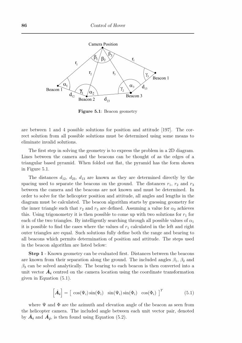
86 Control of Hover
α1
α2
α3
β1 β2
β3
γ1
γ2
γ3
r1
r1
r2 r3
d12
d23
dBeacon 1
Beacon 2Beacon 3
Beacon 1
Camera Position
γ13
Figure 5.1: Beacon geometry
are between 1 and 4 possible solutions for position and attitude [197]. The cor-
rect solution from all possible solutions must be determined using some means to
eliminate invalid solutions.
The first step in solving the geometry is to express the problem in a 2D diagram.
Lines between the camera and the beacons can be thought of as the edges of a
triangular based pyramid. When folded out flat, the pyramid has the form shown
in Figure 5.1.
The distances d12, d23, d13 are known as they are determined directly by the
spacing used to separate the beacons on the ground. The distances r1, r2 and r3between the camera and the beacons are not known and must be determined. In
order to solve for the helicopter position and attitude, all angles and lengths in the
diagram must be calculated. The beacon algorithm starts by guessing geometry for
the inner triangle such that r2 and r3 are defined. Assuming a value for α2 achieves
this. Using trigonometry it is then possible to come up with two solutions for r1 for
each of the two triangles. By intelligently searching through all possible values of α1
it is possible to find the cases where the values of r1 calculated in the left and right
outer triangles are equal. Such solutions fully define both the range and bearing to
all beacons which permits determination of position and attitude. The steps used
in the beacon algorithm are listed below:
Step 1 - Known geometry can be evaluated first. Distances between the beacons
are known from their separation along the ground. The included angles β1, β2 and
β3 can be solved analytically. The bearing to each beacon is then converted into a
unit vector Ai centred on the camera location using the coordinate transformation
given in Equation (5.1).
[Ai
]=[
cos(Ψi) sin(Φi) sin(Ψi) sin(Φi) cos(Φi)]T
(5.1)
where Ψ and Φ are the azimuth and elevation angle of the beacon as seen from
the helicopter camera. The included angle between each unit vector pair, denoted
by Ai and Aj, is then found using Equation (5.2).
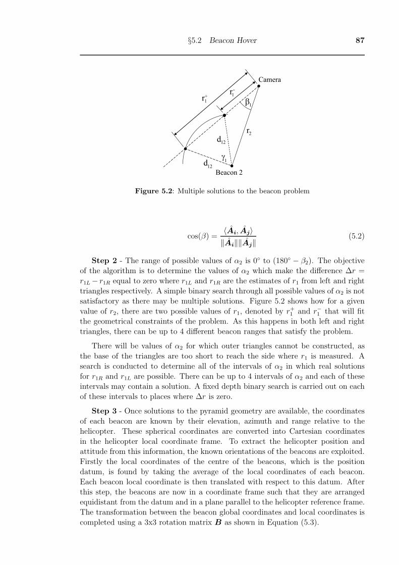
§5.2 Beacon Hover 87
β1
γ1
r2
d12
Beacon 2
Camera
d12
r1+
r1-
Figure 5.2: Multiple solutions to the beacon problem
cos(β) =〈Ai, Aj〉‖Ai‖‖Aj‖
(5.2)
Step 2 - The range of possible values of α2 is 0◦ to (180◦ − β2). The objective
of the algorithm is to determine the values of α2 which make the difference Δr =
r1L− r1R equal to zero where r1L and r1R are the estimates of r1 from left and right
triangles respectively. A simple binary search through all possible values of α2 is not
satisfactory as there may be multiple solutions. Figure 5.2 shows how for a given
value of r2, there are two possible values of r1, denoted by r+1 and r−1 that will fit
the geometrical constraints of the problem. As this happens in both left and right
triangles, there can be up to 4 different beacon ranges that satisfy the problem.
There will be values of α2 for which outer triangles cannot be constructed, as
the base of the triangles are too short to reach the side where r1 is measured. A
search is conducted to determine all of the intervals of α2 in which real solutions
for r1R and r1L are possible. There can be up to 4 intervals of α2 and each of these
intervals may contain a solution. A fixed depth binary search is carried out on each
of these intervals to places where Δr is zero.
Step 3 - Once solutions to the pyramid geometry are available, the coordinates
of each beacon are known by their elevation, azimuth and range relative to the
helicopter. These spherical coordinates are converted into Cartesian coordinates
in the helicopter local coordinate frame. To extract the helicopter position and
attitude from this information, the known orientations of the beacons are exploited.
Firstly the local coordinates of the centre of the beacons, which is the position
datum, is found by taking the average of the local coordinates of each beacon.
Each beacon local coordinate is then translated with respect to this datum. After
this step, the beacons are now in a coordinate frame such that they are arranged
equidistant from the datum and in a plane parallel to the helicopter reference frame.
The transformation between the beacon global coordinates and local coordinates is
completed using a 3x3 rotation matrix B as shown in Equation (5.3).
88 Control of Hover
⎡⎣ x1 x2 x3
y1 y2 y3
z1 z2 z3
⎤⎦local
= B
⎡⎣ x1 x2 x3
y1 y2 y3
z1 z2 z3
⎤⎦global
(5.3)
The positions of the beacons in global coordinates relative to the datum are
known from the constraints of the problem. The beacon positions in local coordi-
nates are the output of the beacon algorithm. Hence the equation above can be
re-arranged to solve for the rotation matrix in terms of the beacon observations and
their known positions as shown in Equation (5.4).
B =
⎡⎣ x1 x2 x3
y1 y2 y3
z1 z2 z3
⎤⎦−1
local
⎡⎣ x1 x2 x3
y1 y2 y3
z1 z2 z3
⎤⎦global
(5.4)
With the rotation matrix defined, the aircraft attitude can be extracted. The
most robust method is to compare elements of the rotation matrix with the quater-
nion representation of B derived from first principles. It can be shown [198] that
the magnitude of each quaternion parameter qi can be expressed in terms of the
main diagonals of the rotation matrix as in Equation (5.5).
4q20 = 1 + b11 + b22 + b33
4q21 = 1 + b11 − b22 − b33
4q22 = 1 − b11 + b22 − b33
4q23 = 1 − b11 − b22 + b33
(5.5)
where bij are the elements of the rotation matrix B. The sign of each quaternion
parameter can be found from the off-diagonal terms in a similar fashion. As an
alternative, Euler angles can also be calculated directly from the rotation matrix,
however, Euler angles are an inferior method of storing attitude since they suffer
from singularities. With attitude determined, the position of the helicopter is found
by rotating the position of the datum point to global coordinates.
Step 4 - Corresponding to each unique set of beacon ranges, will be a helicopter
position and attitude which would produce the same three pairs of elevation and
azimuth angles to target. For example, the set of beacon bearings in table 5.1 gives
rise to the two 6DOF solutions in table 5.2. Clearly, only one solution can be correct
at any one time. The method used to determine which of the 1-4 beacon algorithm
solutions is valid is in two parts. Firstly, a comparison with the inertial attitude is
made. If the beacon attitude differs more than 15◦ from the inertial attitude, it is
discarded. This part is not sufficient by itself, as in some circumstances the beacon
attitude can be very close to the actual attitude, but still be the wrong solution.
Secondly, if more than one solution to the beacon algorithm exists at this point, the
current estimate of position is compared to the solutions. The solution closest to
the current position estimate is then assumed to be correct.
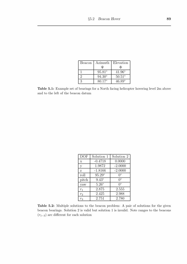
§5.2 Beacon Hover 89
Beacon Azimuth ElevationΨ Φ
1 95.81◦ 41.96◦
2 94.30◦ 50.51◦
3 80.17◦ 46.89◦
Table 5.1: Example set of bearings for a North facing helicopter hovering level 2m above
and to the left of the beacon datum
DOF Solution 1 Solution 2x -0.4718 0.0000y 1.9872 -2.0000z -1.8166 -2.0000roll 95.29◦ 0◦
pitch 9.43◦ 0◦
yaw 5.26◦ 0◦
r1 2.875 2.555r2 2.425 2.988r3 2.751 2.780
Table 5.2: Multiple solutions to the beacon problem: A pair of solutions for the given
beacon bearings. Solution 2 is valid but solution 1 is invalid. Note ranges to the beacons
(r1−3) are different for each solution
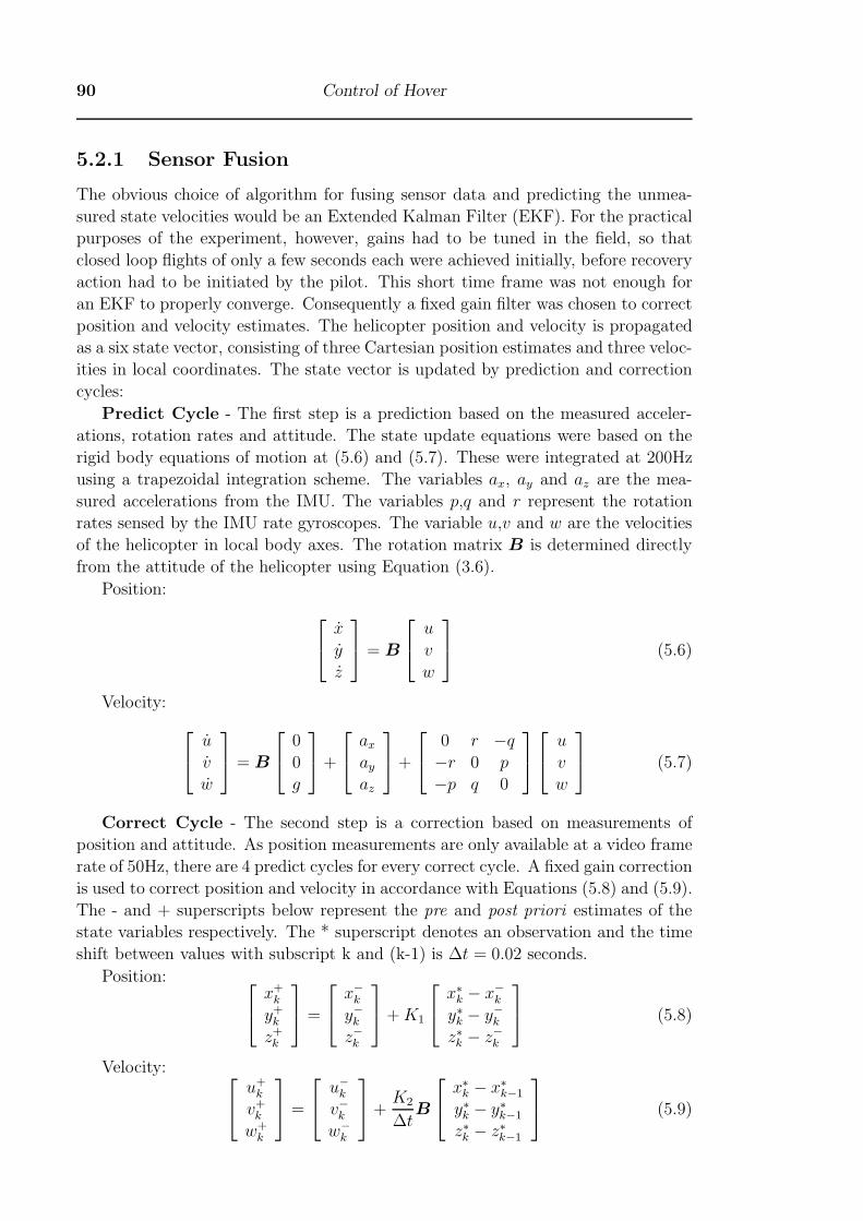
90 Control of Hover
5.2.1 Sensor Fusion
The obvious choice of algorithm for fusing sensor data and predicting the unmea-
sured state velocities would be an Extended Kalman Filter (EKF). For the practical
purposes of the experiment, however, gains had to be tuned in the field, so that
closed loop flights of only a few seconds each were achieved initially, before recovery
action had to be initiated by the pilot. This short time frame was not enough for
an EKF to properly converge. Consequently a fixed gain filter was chosen to correct
position and velocity estimates. The helicopter position and velocity is propagated
as a six state vector, consisting of three Cartesian position estimates and three veloc-
ities in local coordinates. The state vector is updated by prediction and correction
cycles:
Predict Cycle - The first step is a prediction based on the measured acceler-
ations, rotation rates and attitude. The state update equations were based on the
rigid body equations of motion at (5.6) and (5.7). These were integrated at 200Hz
using a trapezoidal integration scheme. The variables ax, ay and az are the mea-
sured accelerations from the IMU. The variables p,q and r represent the rotation
rates sensed by the IMU rate gyroscopes. The variable u,v and w are the velocities
of the helicopter in local body axes. The rotation matrix B is determined directly
from the attitude of the helicopter using Equation (3.6).
Position: ⎡⎣ x
y
z
⎤⎦ = B
⎡⎣ u
v
w
⎤⎦ (5.6)
Velocity: ⎡⎣ u
v
w
⎤⎦ = B
⎡⎣ 0
0
g
⎤⎦+
⎡⎣ axayaz
⎤⎦+
⎡⎣ 0 r −q−r 0 p
−p q 0
⎤⎦⎡⎣ u
v
w
⎤⎦ (5.7)
Correct Cycle - The second step is a correction based on measurements of
position and attitude. As position measurements are only available at a video frame
rate of 50Hz, there are 4 predict cycles for every correct cycle. A fixed gain correction
is used to correct position and velocity in accordance with Equations (5.8) and (5.9).
The - and + superscripts below represent the pre and post priori estimates of the
state variables respectively. The * superscript denotes an observation and the time
shift between values with subscript k and (k-1) is Δt = 0.02 seconds.
Position: ⎡⎣ x+k
y+k
z+k
⎤⎦ =
⎡⎣ x−ky−kz−k
⎤⎦+K1
⎡⎣ x∗k − x−ky∗k − y−kz∗k − z−k
⎤⎦ (5.8)
Velocity: ⎡⎣ u+k
v+k
w+k
⎤⎦ =
⎡⎣ u−kv−kw−k
⎤⎦+K2
ΔtB
⎡⎣ x∗k − x∗k−1
y∗k − y∗k−1
z∗k − z∗k−1
⎤⎦ (5.9)
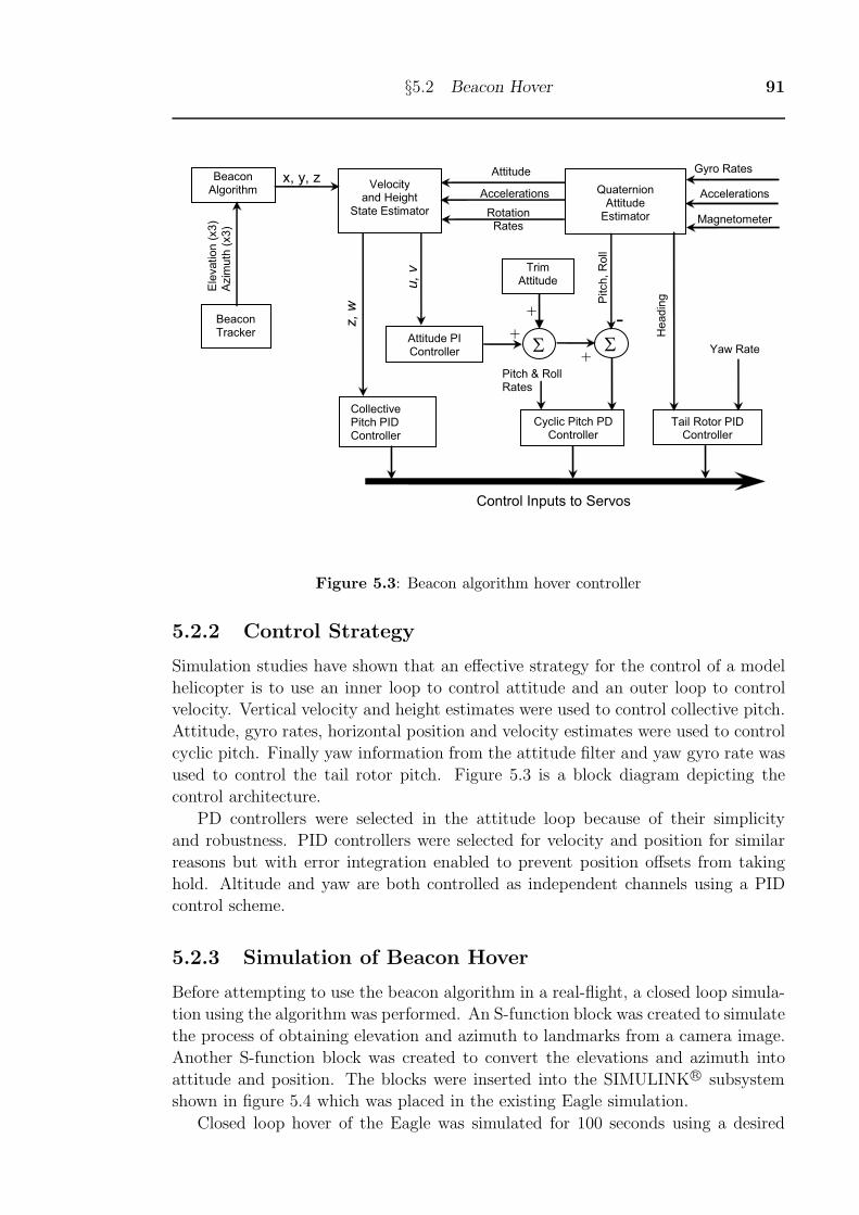
§5.2 Beacon Hover 91
Velocity and Height
State Estimator
Beacon Tracker
Cyclic Pitch PD Controller
Collective Pitch PID Controller
Attitude PI Controller
Quaternion Attitude
Estimator
Trim Attitude
Σ
Tail Rotor PID Controller
Gyro Rates
Magnetometer
Accelerations
Yaw Rate
Headin
g
Pitch, R
oll
Pitch & Roll Rates
u, v
z, w
Accelerations
Attitude
Control Inputs to Servos
Rotation Rates
Beacon Algorithm
+
+
+
- Σ
x, y, z
Ele
vation (
x3)
Azim
uth
(x3)
Figure 5.3: Beacon algorithm hover controller
5.2.2 Control Strategy
Simulation studies have shown that an effective strategy for the control of a model
helicopter is to use an inner loop to control attitude and an outer loop to control
velocity. Vertical velocity and height estimates were used to control collective pitch.
Attitude, gyro rates, horizontal position and velocity estimates were used to control
cyclic pitch. Finally yaw information from the attitude filter and yaw gyro rate was
used to control the tail rotor pitch. Figure 5.3 is a block diagram depicting the
control architecture.
PD controllers were selected in the attitude loop because of their simplicity
and robustness. PID controllers were selected for velocity and position for similar
reasons but with error integration enabled to prevent position offsets from taking
hold. Altitude and yaw are both controlled as independent channels using a PID
control scheme.
5.2.3 Simulation of Beacon Hover
Before attempting to use the beacon algorithm in a real-flight, a closed loop simula-
tion using the algorithm was performed. An S-function block was created to simulate
the process of obtaining elevation and azimuth to landmarks from a camera image.
Another S-function block was created to convert the elevations and azimuth into
attitude and position. The blocks were inserted into the SIMULINKR© subsystem
shown in figure 5.4 which was placed in the existing Eagle simulation.
Closed loop hover of the Eagle was simulated for 100 seconds using a desired
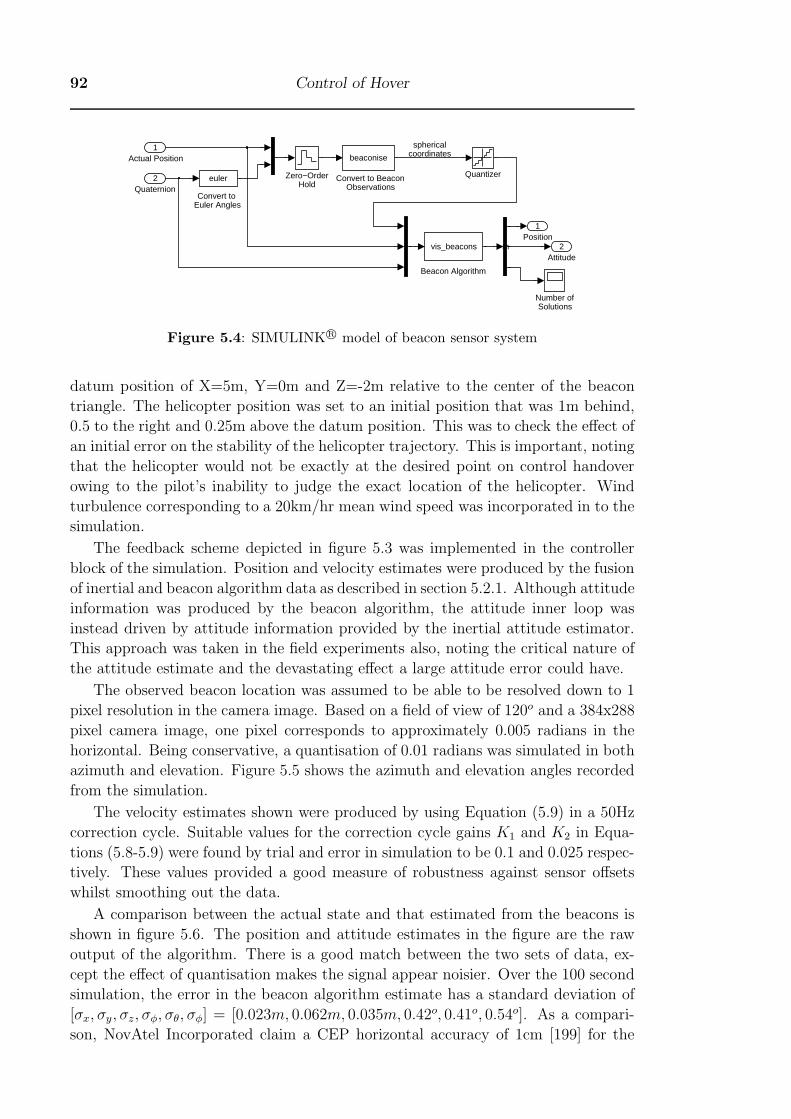
92 Control of Hover
Convert to Euler Angles
Convert to BeaconObservations
Beacon Algorithm
2Attitude
1Position
Zero−OrderHold
euler
vis_beacons
beaconise
Quantizer
Number ofSolutions
emu
2Quaternion
1Actual Position
sphericalcoordinates
Figure 5.4: SIMULINK R© model of beacon sensor system
datum position of X=5m, Y=0m and Z=-2m relative to the center of the beacon
triangle. The helicopter position was set to an initial position that was 1m behind,
0.5 to the right and 0.25m above the datum position. This was to check the effect of
an initial error on the stability of the helicopter trajectory. This is important, noting
that the helicopter would not be exactly at the desired point on control handover
owing to the pilot’s inability to judge the exact location of the helicopter. Wind
turbulence corresponding to a 20km/hr mean wind speed was incorporated in to the
simulation.
The feedback scheme depicted in figure 5.3 was implemented in the controller
block of the simulation. Position and velocity estimates were produced by the fusion
of inertial and beacon algorithm data as described in section 5.2.1. Although attitude
information was produced by the beacon algorithm, the attitude inner loop was
instead driven by attitude information provided by the inertial attitude estimator.
This approach was taken in the field experiments also, noting the critical nature of
the attitude estimate and the devastating effect a large attitude error could have.
The observed beacon location was assumed to be able to be resolved down to 1
pixel resolution in the camera image. Based on a field of view of 120o and a 384x288
pixel camera image, one pixel corresponds to approximately 0.005 radians in the
horizontal. Being conservative, a quantisation of 0.01 radians was simulated in both
azimuth and elevation. Figure 5.5 shows the azimuth and elevation angles recorded
from the simulation.
The velocity estimates shown were produced by using Equation (5.9) in a 50Hz
correction cycle. Suitable values for the correction cycle gains K1 and K2 in Equa-
tions (5.8-5.9) were found by trial and error in simulation to be 0.1 and 0.025 respec-
tively. These values provided a good measure of robustness against sensor offsets
whilst smoothing out the data.
A comparison between the actual state and that estimated from the beacons is
shown in figure 5.6. The position and attitude estimates in the figure are the raw
output of the algorithm. There is a good match between the two sets of data, ex-
cept the effect of quantisation makes the signal appear noisier. Over the 100 second
simulation, the error in the beacon algorithm estimate has a standard deviation of
[σx, σy, σz, σφ, σθ, σφ] = [0.023m, 0.062m, 0.035m, 0.42o, 0.41o, 0.54o]. As a compari-
son, NovAtel Incorporated claim a CEP horizontal accuracy of 1cm [199] for the
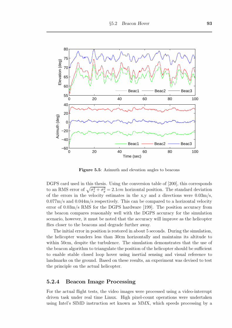
§5.2 Beacon Hover 93
0 20 40 60 80 10055
60
65
70
75
80
Ele
vatio
n (d
eg)
Beac1 Beac2 Beac3
0 20 40 60 80 100−60
−40
−20
0
20
40
Azi
mut
h (d
eg)
Time (sec)
Beac1 Beac2 Beac3
Figure 5.5: Azimuth and elevation angles to beacons
DGPS card used in this thesis. Using the conversion table of [200], this corresponds
to an RMS error of√σ2x + σ2
y = 2.1cm horizontal position. The standard deviation
of the errors in the velocity estimates in the x,y and z directions were 0.03m/s,
0.077m/s and 0.044m/s respectively. This can be compared to a horizontal velocity
error of 0.03m/s RMS for the DGPS hardware [199]. The position accuracy from
the beacon compares reasonably well with the DGPS accuracy for the simulation
scenario, however, it must be noted that the accuracy will improve as the helicopter
flies closer to the beacons and degrade further away.
The initial error in position is restored in about 5 seconds. During the simulation,
the helicopter wanders less than 30cm horizontally and maintains its altitude to
within 50cm, despite the turbulence. The simulation demonstrates that the use of
the beacon algorithm to triangulate the position of the helicopter should be sufficient
to enable stable closed loop hover using inertial sensing and visual reference to
landmarks on the ground. Based on these results, an experiment was devised to test
the principle on the actual helicopter.
5.2.4 Beacon Image Processing
For the actual flight tests, the video images were processed using a video-interrupt
driven task under real time Linux. High pixel-count operations were undertaken
using Intel’s SIMD instruction set known as MMX, which speeds processing by a
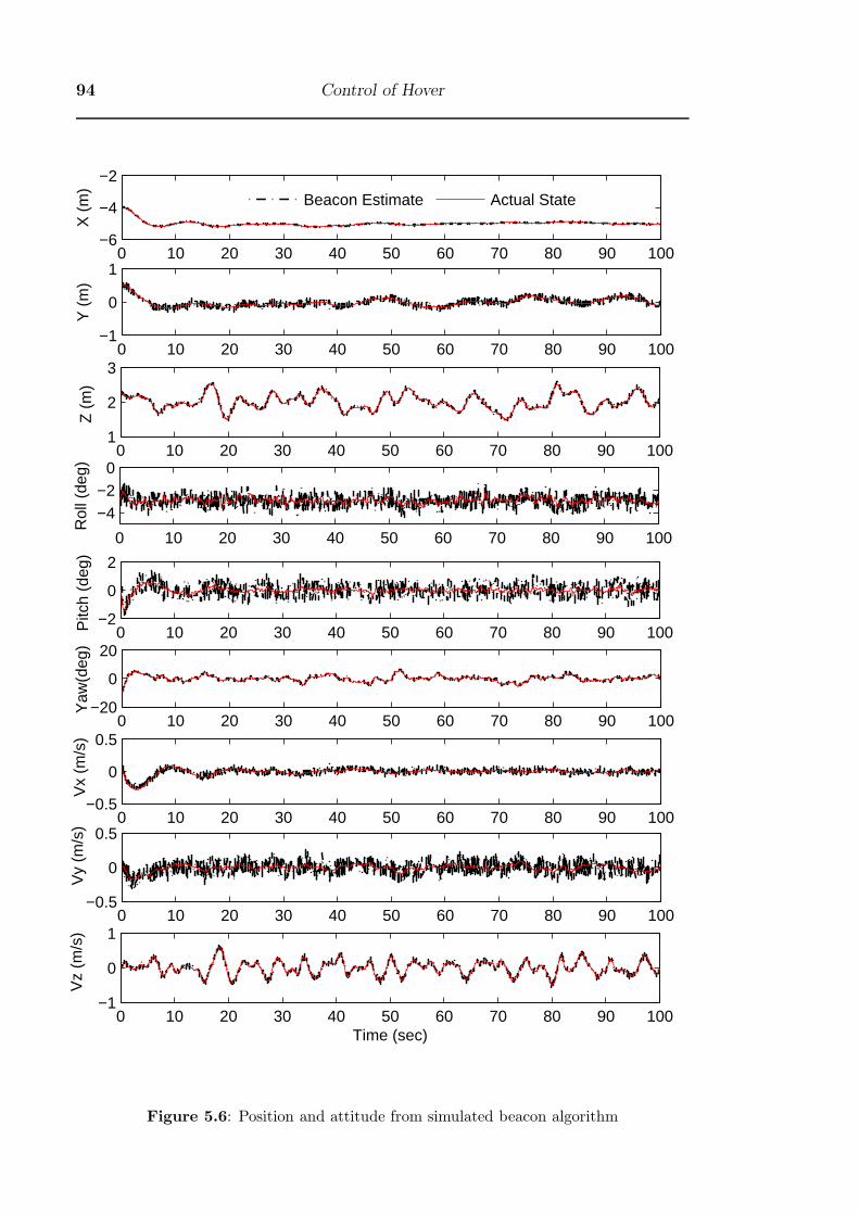
94 Control of Hover
0 10 20 30 40 50 60 70 80 90 100−6
−4
−2
X (
m)
Beacon Estimate Actual State
0 10 20 30 40 50 60 70 80 90 100−1
0
1
Y (
m)
0 10 20 30 40 50 60 70 80 90 1001
2
3
Z (
m)
0 10 20 30 40 50 60 70 80 90 100
−4−2
0
Rol
l (de
g)
0 10 20 30 40 50 60 70 80 90 100−2
0
2
Pitc
h (d
eg)
0 10 20 30 40 50 60 70 80 90 100−20
0
20
Yaw
(deg
)
0 10 20 30 40 50 60 70 80 90 100−0.5
0
0.5
Vx
(m/s
)
0 10 20 30 40 50 60 70 80 90 100−0.5
0
0.5
Vy
(m/s
)
0 10 20 30 40 50 60 70 80 90 100−1
0
1
Vz
(m/s
)
Time (sec)
Figure 5.6: Position and attitude from simulated beacon algorithm

§5.2 Beacon Hover 95
factor of four over the normal instruction set. The image size was 344x288 pixels.
The camera was an inexpensive security camera rated at 400 TV lines with a compa-
rable wide-angle lens giving a horizontal field of view of 120◦. Due to the inexpensive
nature of the optics, the image produced by the system was highly distorted and
unacceptable for this precision positioning application. In order to overcome these
issues, Tsai’s camera calibration algorithm [201,202] was applied. A non-linear op-
timisation of camera radial distortion parameters is performed based on comparing
ideal pixel locations to measured pixel positions. Using this technique, there was
no sign of visible distortion in the image. Rather than apply a look-up-table to the
entire image on every frame, all coordinates measured from the screen were trans-
formed by the camera calibration parameters prior to passing the data to the beacon
solution.
The images were initially pre-processed using a centre surround also known as
Mexican hat operator [203], which is essentially a bandpass filter on the image.
The effect of this operator was to remove regions of the image that did not contain
high contrast. The beacons were made from styrofoam, and were thus very bright.
Certain sites where testing was undertaken were very bright in the near infrared
wavelengths, as is typical of vegetation in sunlight. Short pass filters were placed
over the camera to accentuate the intensity of the beacons. The filters used did not
cut wavelengths longer than 700nm (Kodak Wratten filters), so only undesirable
visible wavelengths could be blocked.
After pre-processing to eliminate regions of no contrast, a threshold was applied
to segment the beacons from the background. Figure 5.7 shows a typical view of
the beacons from the helicopter during a hover trial and a view of the beacons after
a threshold has been applied. Due to the contamination with IR, thresholds of as
little as 16 out of 256 grey levels were used, rather than the expected 40 or 50. Since
the essential configuration of the beacons was known, it was possible for the tracking
system to search for the beacons from the bottom of the screen towards the top,
labelling the beacons in sequence. In order to qualify as being a beacon, a certain
threshold number of white pixels was required to be within a 60x60 pixel window.
The size of each beacon was measured based on the first moment of intensity (ie.
measuring only white pixels) within each tracking window.
The tracking system was a standard alpha, beta, gamma tracker, with online
adjustable tracking parameters [204]. Values of alpha, beta and gamma of 1, 0,
and 0.04 were found to be successful, and no modifications were made after early
tests. Essentially the tracking stage was not required. In addition to position, the
size of each window was also tracked while tracking, so as to reduce the effect of
additional ‘speckle’ (particularly dandelions) around the beacons. The window size
was adjusted by assuming that the beacon was elliptical, and thus that the first
moment in each major axis would define the shape. The size of the window was
adjusted to be 1.2 times the size of the moments of the beacon, on each major axis.
Track parameters for the window resizing operation were an alpha of 0.1 and the
other parameters all zero. Using this system, track was held for all beacons under
almost all situations until a beacon departed the 120◦ field of view of the camera.
The beacon tracking system converts the 2D Cartesian screen coordinates deter-
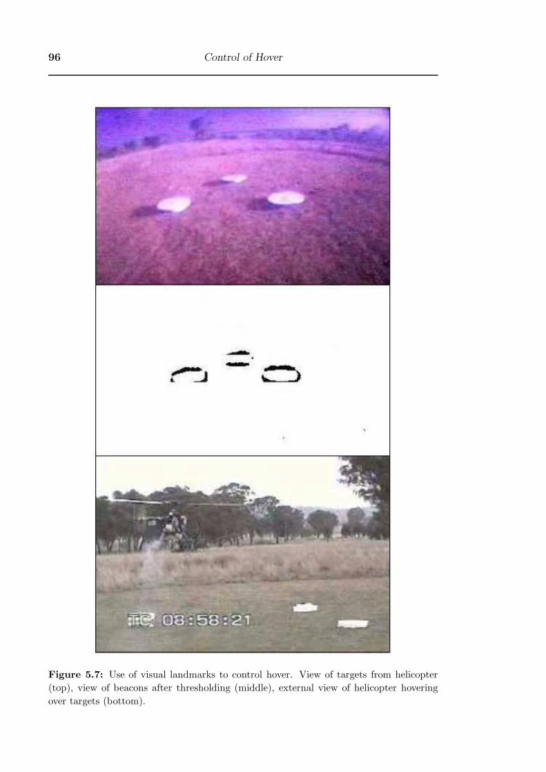
96 Control of Hover
Figure 5.7: Use of visual landmarks to control hover. View of targets from helicopter
(top), view of beacons after thresholding (middle), external view of helicopter hovering
over targets (bottom).
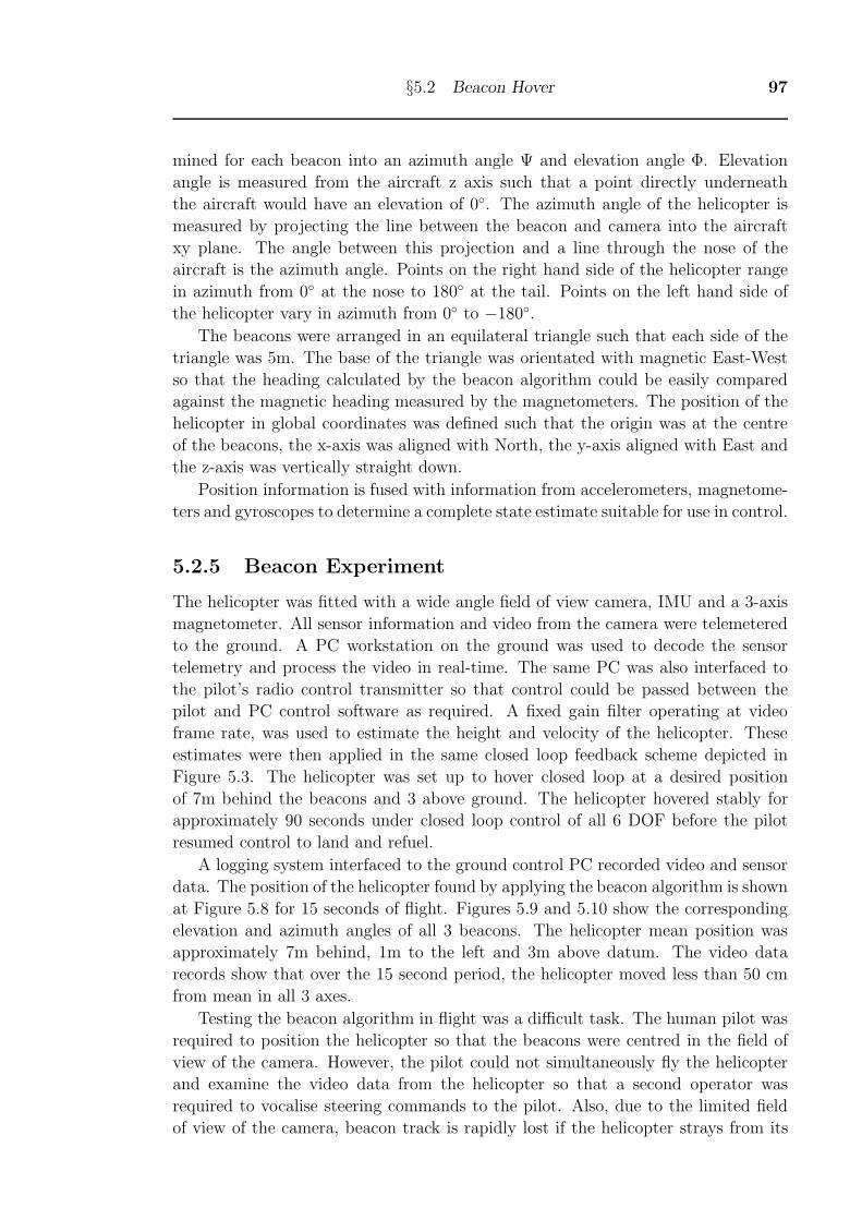
§5.2 Beacon Hover 97
mined for each beacon into an azimuth angle Ψ and elevation angle Φ. Elevation
angle is measured from the aircraft z axis such that a point directly underneath
the aircraft would have an elevation of 0◦. The azimuth angle of the helicopter is
measured by projecting the line between the beacon and camera into the aircraft
xy plane. The angle between this projection and a line through the nose of the
aircraft is the azimuth angle. Points on the right hand side of the helicopter range
in azimuth from 0◦ at the nose to 180◦ at the tail. Points on the left hand side of
the helicopter vary in azimuth from 0◦ to −180◦.The beacons were arranged in an equilateral triangle such that each side of the
triangle was 5m. The base of the triangle was orientated with magnetic East-West
so that the heading calculated by the beacon algorithm could be easily compared
against the magnetic heading measured by the magnetometers. The position of the
helicopter in global coordinates was defined such that the origin was at the centre
of the beacons, the x-axis was aligned with North, the y-axis aligned with East and
the z-axis was vertically straight down.
Position information is fused with information from accelerometers, magnetome-
ters and gyroscopes to determine a complete state estimate suitable for use in control.
5.2.5 Beacon Experiment
The helicopter was fitted with a wide angle field of view camera, IMU and a 3-axis
magnetometer. All sensor information and video from the camera were telemetered
to the ground. A PC workstation on the ground was used to decode the sensor
telemetry and process the video in real-time. The same PC was also interfaced to
the pilot’s radio control transmitter so that control could be passed between the
pilot and PC control software as required. A fixed gain filter operating at video
frame rate, was used to estimate the height and velocity of the helicopter. These
estimates were then applied in the same closed loop feedback scheme depicted in
Figure 5.3. The helicopter was set up to hover closed loop at a desired position
of 7m behind the beacons and 3 above ground. The helicopter hovered stably for
approximately 90 seconds under closed loop control of all 6 DOF before the pilot
resumed control to land and refuel.
A logging system interfaced to the ground control PC recorded video and sensor
data. The position of the helicopter found by applying the beacon algorithm is shown
at Figure 5.8 for 15 seconds of flight. Figures 5.9 and 5.10 show the corresponding
elevation and azimuth angles of all 3 beacons. The helicopter mean position was
approximately 7m behind, 1m to the left and 3m above datum. The video data
records show that over the 15 second period, the helicopter moved less than 50 cm
from mean in all 3 axes.
Testing the beacon algorithm in flight was a difficult task. The human pilot was
required to position the helicopter so that the beacons were centred in the field of
view of the camera. However, the pilot could not simultaneously fly the helicopter
and examine the video data from the helicopter so that a second operator was
required to vocalise steering commands to the pilot. Also, due to the limited field
of view of the camera, beacon track is rapidly lost if the helicopter strays from its
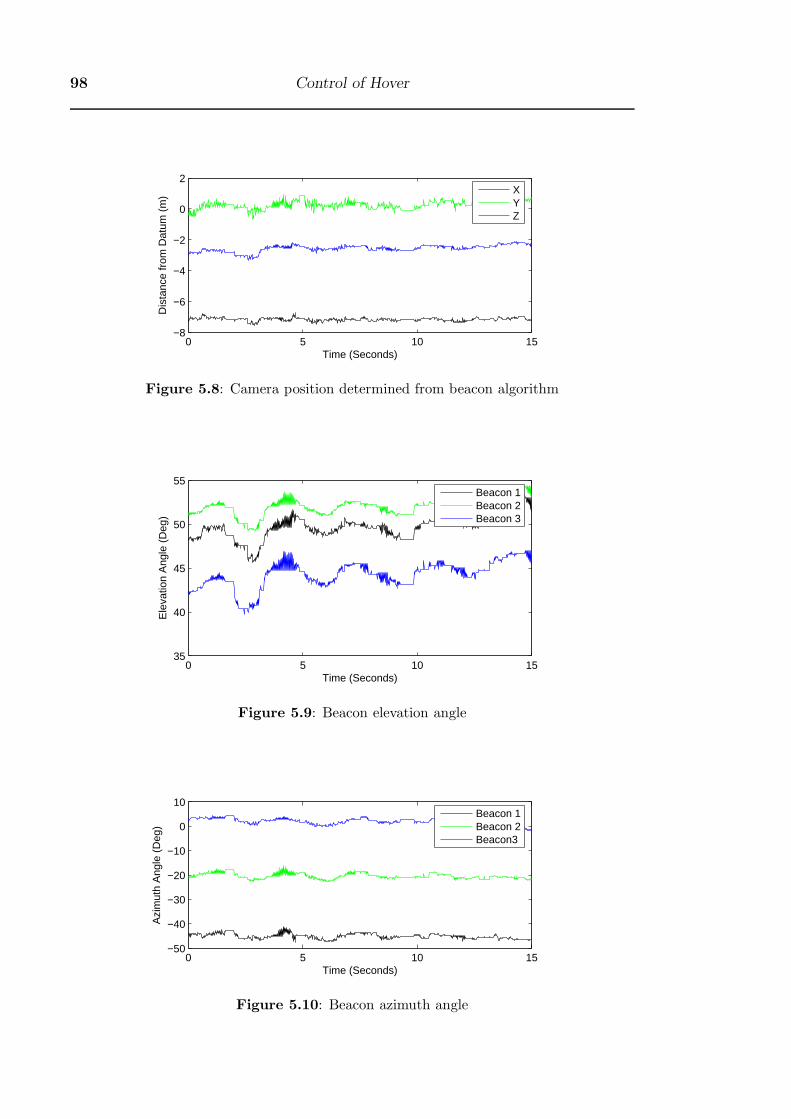
98 Control of Hover
0 5 10 15−8
−6
−4
−2
0
2
Time (Seconds)
Dis
tanc
e fr
om D
atum
(m
)
XYZ
Figure 5.8: Camera position determined from beacon algorithm
0 5 10 1535
40
45
50
55
Time (Seconds)
Ele
vatio
n A
ngle
(D
eg)
Beacon 1Beacon 2Beacon 3
Figure 5.9: Beacon elevation angle
0 5 10 15−50
−40
−30
−20
−10
0
10
Time (Seconds)
Azi
mut
h A
ngle
(D
eg)
Beacon 1Beacon 2Beacon3
Figure 5.10: Beacon azimuth angle
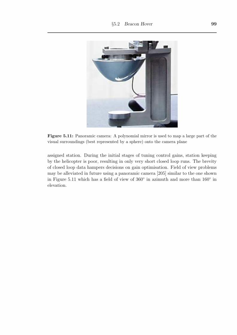
§5.2 Beacon Hover 99
Figure 5.11: Panoramic camera: A polynomial mirror is used to map a large part of the
visual surroundings (best represented by a sphere) onto the camera plane
assigned station. During the initial stages of tuning control gains, station keeping
by the helicopter is poor, resulting in only very short closed loop runs. The brevity
of closed loop data hampers decisions on gain optimisation. Field of view problems
may be alleviated in future using a panoramic camera [205] similar to the one shown
in Figure 5.11 which has a field of view of 360◦ in azimuth and more than 160◦ in
elevation.
100 Control of Hover
5.3 Optic Flow Damped Hover
In this section, an optic flow based hover and landing system is presented which
provides a means to land in an unknown environment without a reliance on GPS or
other navigation aids. The sensor is used to reduce the lateral and longitudinal drift
of the helicopter to negligible rates so that a safe landing can take place without an
absolute position reference. An operational scenario could be envisaged where an
unmanned helicopter could first search for a suitable landing area using visual or
other means. During the search, terrain clearance could be maintained with sensing
based on visual, laser range finding or radar systems. As aprt of other research,
I have developed a novel laser ranging system [195] that determines the slope and
distance of the ground in one 40 millisecond scan using a conical scan pattern. This
sensor could be used to search for a piece of ground that was level enough to land
on, and then, in combination with the optic flow sensor, an automated landing
could be executed. The optic flow and inertial sensor compliment each other well.
The optic flow provides a noisy measurement of horizontal velocity which does not
suffer from offsets. When integrated, the accelerations match the velocity well but
due to slight offsets, the integrated velocity diverges quickly if not corrected by a
separate measure of velocity. Accelerometers suffer offsets due to thermal effects,
misalignment and calibration errors. By combining the integrated inertial data with
the vision sensing, the noise of the optic flow measurement can be smoothed whilst
simultaneously compensating for offsets in the measured accelerations.
Optic flow can result from translations and rotations. For a downwards looking
camera, like the one used here, the effect of positive (nose-up) pitch rate q is the same
as the effect of forward velocity. Likewise, the effect of positive roll rate p (right wing
down) is the same as lateral translation to the left. In these cases, for a relatively
planar surface under the helicopter, the entire image is translated by the motion.
The effect of yaw is to produce an image flow field consisting of vectors rotated
around the point in the image corresponding to the center of rotation. Without any
translation, the average of these vectors cancels out. Also, during hover, yaw rates
are kept relatively small by the heading control loop which is very effective. Yaw
can therefore be ignored in calculating the lateral and longitudinal drift. Likewise
the effect of vertical motion results in image loom, however, due to the collective
control loop, the vertical velocity are very small (3cm/sec for autoland) and can be
neglected. Using an inertial system, the effect of rotations can be removed simply
by subtracting the rotations rates measured by onboard rate gyroscopes. The net
remaining angular motion of the image is proportional to the horizontal velocity. In
terms of the components of motion, we can express the longitudinal u and lateral
v velocities in terms of the helicopter height above ground level H and the flow
components Qx and Qy as in Equation (5.10). In these equations, the flow is defined
to be positive when it corresponds to a positive translation along one of the helicopter
body axes.
u = (Qx − q)H v = (Qy + p)H (5.10)
The Yamaha attitude system (YAS) outputs pitch angle (θ), roll angle (φ), roll

§5.3 Optic Flow Damped Hover 101
rate (p), pitch rate (q) and yaw rate (r). The YAS also outputs the net accelerations
[ax, ay, az] sensed in the body axes coordinates after the gravitational acceleration
vector has been subtracted. The offsets from these sensors are relatively small, less
than 0.05m/s2 in acceleration and 0.1 deg/sec in rotation rates. I have previously
described an Extended Kalman Filter [26] which enables the accelerometer offsets
to be estimated online. This was for a low grade IMU on a very small helicopter
which suffered from significant sensor offsets and drift. For the RMAX, this extra
complexity is not required and a simpler complimentary filter has been applied. This
is a similar approach to that taken by Corke in [206] to fuse optic flow data with
inertials on a small helicopter. The fusion of inertial and optic flow information
takes part in two parts consisting of a state update phase and then a correction
phase:
Predict Cycle - The first step is a prediction based on the measured accelerations,
rotation rates and attitude. The state update equations were based on the rigid
body motion Equations (5.11). These were integrated at 100Hz using a trapezoidal
integrations scheme. The variables ax, ay and az are the measured accelerations
from the IMU. The variables p,q and r represent the rotation rates sensed by the
IMU rate gyroscopes. The variable u,v and w are the velocities of the helicopter in
local body axes. ⎡⎣ u
v
w
⎤⎦ =
⎡⎣ axayaz
⎤⎦+
⎡⎣ 0 r −q−r 0 p
−p q 0
⎤⎦⎡⎣ u
v
w
⎤⎦ (5.11)
Correct Cycle - The second step is a correction based on measurements of the
optic flow and height. As optic flow measurements are only available at a video
frame rate of 50Hz, there are 2 predict cycles for every correct cycle. A fixed gain
correction is used to correct velocity in accordance with Equation (5.12) . The -
and + superscripts below represent the pre and post priori estimates of the state
variables respectively. The * superscript denotes an observation and the time shift
between values with subscript k and (k-1) is t = 0.02 seconds. The vertical velocity
is corrected from the GPS vertical velocity output or from the derivative of the
laser-range finder height, depending on which sensor is being used at the time.[u+k
v+k
]=
[u−kv−k
]+ α
[Q∗xH
∗ − u−kQ∗yH
∗ − v−k
](5.12)
A value of 0.25 was used for the gain α. This was thought to be an adequate
compromise between smoothing out noise in the sensor and minimising the effect of
accelerometer drift.
The helicopter was flown at a height of approximately 1m above a grass field
with no artificial texture in view of the camera. Once the helicopter was established
in a reasonably stable hover by the pilot on the ground, control was switched to
the flight computer. GPS altitude was used to control the height of the helicopter
by varying the collective pitch using a PI controller. The height of the helicopter
was regulated to within 10cm of the set height. The aileron and elevator inputs
were controlled by PI control loops using the lateral and longitudinal velocities
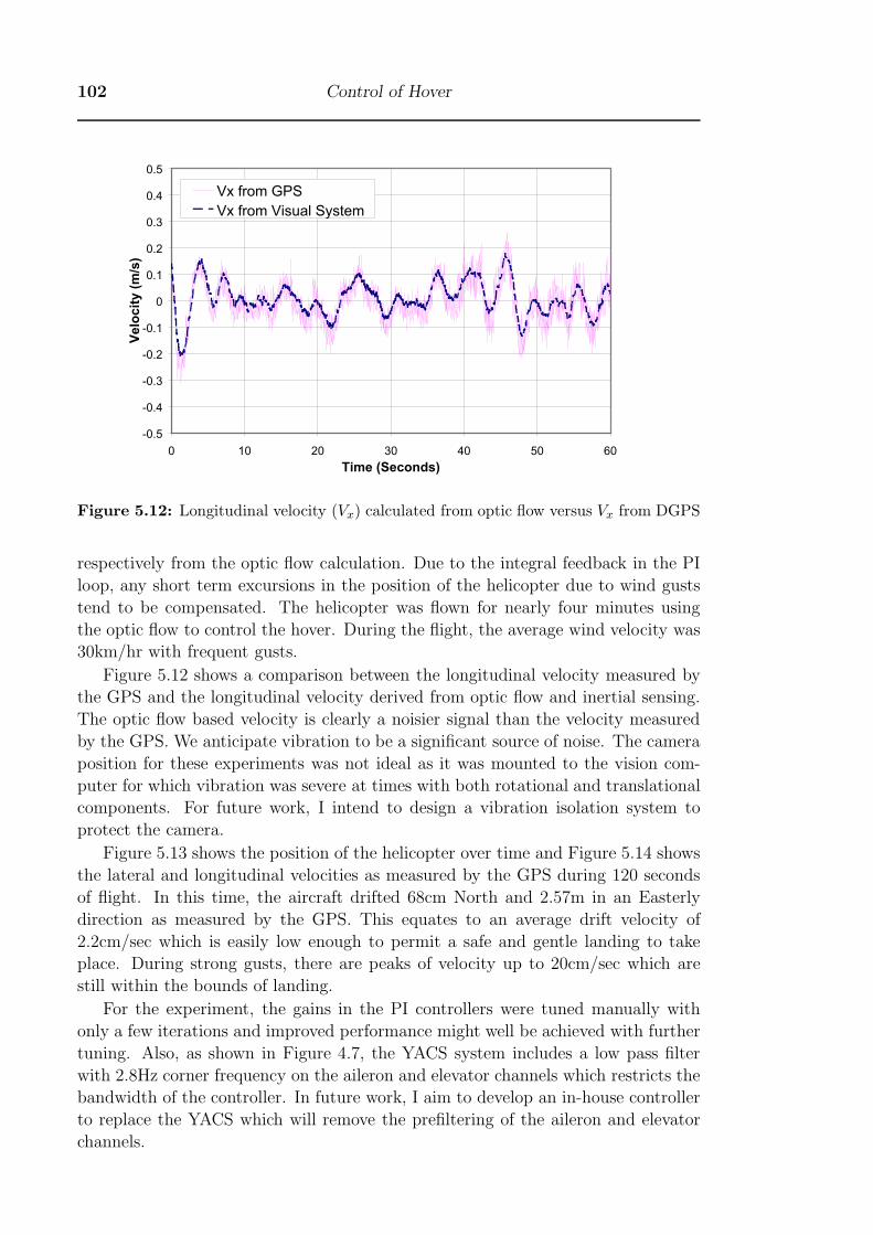
102 Control of Hover
-0.5
-0.4
-0.3
-0.2
-0.1
0
0.1
0.2
0.3
0.4
0.5
0 10 20 30 40 50 60
Time (Seconds)
Velo
cit
y (
m/s
)
Vx from GPS
Vx from Visual System
Figure 5.12: Longitudinal velocity (Vx) calculated from optic flow versus Vx from DGPS
respectively from the optic flow calculation. Due to the integral feedback in the PI
loop, any short term excursions in the position of the helicopter due to wind gusts
tend to be compensated. The helicopter was flown for nearly four minutes using
the optic flow to control the hover. During the flight, the average wind velocity was
30km/hr with frequent gusts.
Figure 5.12 shows a comparison between the longitudinal velocity measured by
the GPS and the longitudinal velocity derived from optic flow and inertial sensing.
The optic flow based velocity is clearly a noisier signal than the velocity measured
by the GPS. We anticipate vibration to be a significant source of noise. The camera
position for these experiments was not ideal as it was mounted to the vision com-
puter for which vibration was severe at times with both rotational and translational
components. For future work, I intend to design a vibration isolation system to
protect the camera.
Figure 5.13 shows the position of the helicopter over time and Figure 5.14 shows
the lateral and longitudinal velocities as measured by the GPS during 120 seconds
of flight. In this time, the aircraft drifted 68cm North and 2.57m in an Easterly
direction as measured by the GPS. This equates to an average drift velocity of
2.2cm/sec which is easily low enough to permit a safe and gentle landing to take
place. During strong gusts, there are peaks of velocity up to 20cm/sec which are
still within the bounds of landing.
For the experiment, the gains in the PI controllers were tuned manually with
only a few iterations and improved performance might well be achieved with further
tuning. Also, as shown in Figure 4.7, the YACS system includes a low pass filter
with 2.8Hz corner frequency on the aileron and elevator channels which restricts the
bandwidth of the controller. In future work, I aim to develop an in-house controller
to replace the YACS which will remove the prefiltering of the aileron and elevator
channels.

§5.3 Optic Flow Damped Hover 103
-4
-3
-2
-1
0
1
2
3
4
0 10 20 30 40 50 60 70 80 90 100 110 120
Time (Seconds)
Dis
tan
ce T
ravelled
(m
)
Northings
Eastings
Figure 5.13: Helicopter position during closed loop hover
-1
-0.8
-0.6
-0.4
-0.2
0
0.2
0.4
0.6
0.8
1
0 20 40 60 80 100 120
Time (Seconds)
Velo
cit
y (
m/s
)
Vx
Vy
Figure 5.14: Helicopter longitudinal (Vx) and lateral (Vy) velocities measured by DGPS
during closed loop hover
104 Control of Hover
5.4 Summary
Visual sensing provides a cheap, lightweight and passive way of controlling hover or
low speed flight in an autonomous flying vehicle. A method using triangulation of
postion in three dimensions from visual bearings to landmarks was used succesfully
to control a helicopter in hover.
Chapter 6
Control of Forward Flight
6.1 Introduction
A number of researchers have suggested that insects use optic flow in forward flight
to control their terrain clearance [8–10]. The aim of this chapter is to show, in
simulation and experimentally, that calculation of range from optic flow can also
be used to avoid terrain by an inherently unstable rotorcraft. Experiments were
completed with both the Eagle helicopter and the RMAX helicopter. The concept
was first tested in closed loop on a relatively flat surface using the control by teleme-
try scheme on an Eagle helicopter. Later, the RMAX helicopter completed terrain
following experiments over a more irregular landscape using all onboard processing.
The tests in this chapter make use of a downwards looking camera that measures
the optic flow of the ground underneath the helicopter. If speed is known, the terrain
clearance (H) can be calculated from Equation (6.1) where V is the horizontal
speed of the helicopter and Q is the magnitude of the optic flow vector due to pure
translation. The basic assumption in this work is that the ground speed of the
vehicle is known approximately. In our case, the speed of the helicopter is known
from GPS measurements or from the observed open loop behaviour of the helicopter.
H = V/Q (6.1)
6.2 Sensor Fusion
Equation (6.1) can be used to measure height above terrain. This estimate tends
to be rather noisy owing to the vibration of the platform and the resulting noise in
the optic flow measurement. To reduce the effects of vibration, the optic flow and
velocity data are both smoothed using a moving average filter comprising 5 samples,
before the velocity is divided by the optic flow to get range. Figure 6.1 shows ground
speed and optic flow range versus time for the same period of flight for the RMAX
helicopter flying over a rough grass paddock. The output of the laser rangefinder
(LRF) is provided as a benchmark. The optic flow range is calculated by dividing
the longitudinal velocity by the longitudinal optic flow after applying the averaging
filter. The plot of standard deviation in figure 6.1 was calculated using a sliding
window of 50 samples (i.e. 1 second) width applied to the discrepancy between the
optic flow range and the LRF. At 5m/s the standard deviation of the noise is about
105
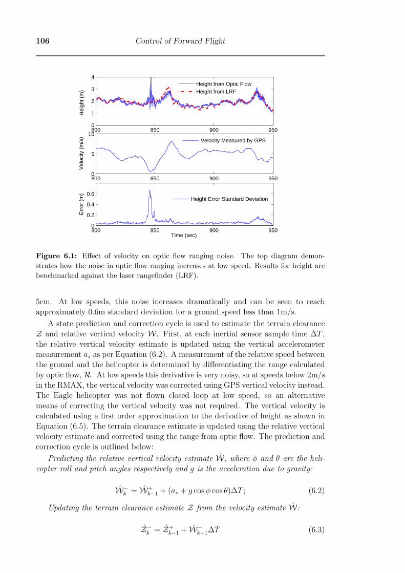
106 Control of Forward Flight
800 850 900 9500
1
2
3
4H
eigh
t (m
)Height from Optic FlowHeight from LRF
800 850 900 9500
5
10
Vel
ocity
(m
/s)
Velocity Measured by GPS
800 850 900 9500
0.2
0.4
0.6
Err
or (
m)
Time (sec)
Height Error Standard Deviation
Figure 6.1: Effect of velocity on optic flow ranging noise. The top diagram demon-
strates how the noise in optic flow ranging increases at low speed. Results for height are
benchmarked against the laser rangefinder (LRF).
5cm. At low speeds, this noise increases dramatically and can be seen to reach
approximately 0.6m standard deviation for a ground speed less than 1m/s.
A state prediction and correction cycle is used to estimate the terrain clearance
Z and relative vertical velocity W. First, at each inertial sensor sample time ΔT ,
the relative vertical velocity estimate is updated using the vertical accelerometer
measurement az as per Equation (6.2). A measurement of the relative speed between
the ground and the helicopter is determined by differentiating the range calculated
by optic flow, R. At low speeds this derivative is very noisy, so at speeds below 2m/s
in the RMAX, the vertical velocity was corrected using GPS vertical velocity instead.
The Eagle helicopter was not flown closed loop at low speed, so an alternative
means of correcting the vertical velocity was not required. The vertical velocity is
calculated using a first order approximation to the derivative of height as shown in
Equation (6.5). The terrain clearance estimate is updated using the relative vertical
velocity estimate and corrected using the range from optic flow. The prediction and
correction cycle is outlined below:
Predicting the relative vertical velocity estimate W, where φ and θ are the heli-
copter roll and pitch angles respectively and g is the acceleration due to gravity:
W−k = W+
k−1 + (az + g cos φ cos θ)ΔT ; (6.2)
Updating the terrain clearance estimate Z from the velocity estimate W:
Z−k = Z+
k−1 + W−k−1ΔT (6.3)
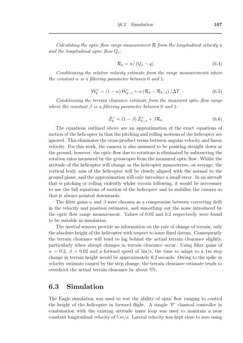
§6.3 Simulation 107
Calculating the optic flow range measurement R from the longitudinal velocity u
and the longitudinal optic flow Qx:
Rk = u/ (Qx − q) (6.4)
Conditioning the relative velocity estimate from the range measurements where
the constant α is a filtering parameter between 0 and 1:
W+k = (1 − α) W−
k−1 + α (Rk −Rk−1) /ΔT (6.5)
Conditioning the terrain clearance estimate from the measured optic flow range
where the constant β is a filtering parameter between 0 and 1:
Z+k = (1 − β) Z+
k−1 + βRk (6.6)
The equations outlined above are an approximation of the exact equations of
motion of the helicopter in that the pitching and rolling motions of the helicopter are
ignored. This eliminates the cross-product terms between angular velocity and linear
velocity. For this work, the camera is also assumed to be pointing straight down at
the ground, however, the optic flow due to rotations is eliminated by subtracting the
rotation rates measured by the gyroscopes from the measured optic flow. Whilst the
attitude of the helicopter will change as the helicopter manoeuvres, on average, the
vertical body axis of the helicopter will be closely aligned with the normal to the
ground plane, and the approximation will only introduce a small error. In an aircraft
that is pitching or rolling violently whilst terrain following, it would be neccessary
to use the full equations of motion of the helicopter and to stabilise the camera so
that it always pointed downwards.
The filter gains α and β were choosen as a compromise between correcting drift
in the velocity and position estimates, and smoothing out the noise introduced by
the optic flow range measurement. Values of 0.02 and 0.2 respectively were found
to be suitable in simulation.
The inertial sensors provide no information on the rate of change of terrain, only
the absolute height of the helicopter with respect to some fixed datum. Consequently
the terrain clearance will tend to lag behind the actual terrain clearance slightly,
particularly when abrupt changes in terrain clearance occur. Using filter gains of
α = 0.2, β = 0.02 and a forward speed of 5m/s, the time to adapt to a 1m step
change in terrain height would be approximately 0.2 seconds. Owing to the spike in
velocity estimate caused by the step change, the terrain clearance estimate tends to
overshoot the actual terrain clearance by about 5%.
6.3 Simulation
The Eagle simulation was used to test the ability of optic flow ranging to control
the height of the helicopter in forward flight. A simple ’P’ classical controller in
combination with the existing attitude inner loop was used to maintain a near
constant longitudinal velocity of 5m/s. Lateral velocity was kept close to zero using
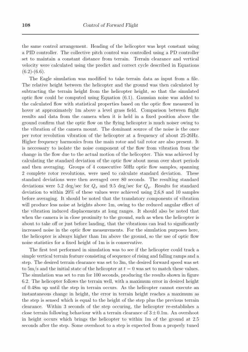
108 Control of Forward Flight
the same control arrangement. Heading of the helicopter was kept constant using
a PID controller. The collective pitch control was controlled using a PD controller
set to maintain a constant distance from terrain. Terrain clearance and vertical
velocity were calculated using the predict and correct cycle described in Equations
(6.2)-(6.6).
The Eagle simulation was modified to take terrain data as input from a file.
The relative height between the helicopter and the ground was then calculated by
subtracting the terrain height from the helicopter height, so that the simulated
optic flow could be computed using Equation (6.1). Gaussian noise was added to
the calculated flow with statistical properties based on the optic flow measured in
hover at approximately 1m above a level grass field. Comparison between flight
results and data from the camera when it is held in a fixed position above the
ground confirm that the optic flow on the flying helicopter is much noiser owing to
the vibration of the camera mount. The dominant source of the noise is the once
per rotor revolution vibration of the helicopter at a frequency of about 25-26Hz.
Higher frequency harmonics from the main rotor and tail rotor are also present. It
is neccessary to isolate the noise component of the flow from vibration from the
change in the flow due to the actual motion of the helicopter. This was achieved by
calculating the standard deviation of the optic flow about mean over short periods
and then averaging. Groups of 4 consecutive 50Hz optic flow samples, spanning
2 complete rotor revolutions, were used to calculate standard deviation. These
standard deviations were then averaged over 80 seconds. The resulting standard
deviations were 5.2 deg/sec for Qx and 9.5 deg/sec for Qy. Results for standard
deviation to within 20% of these values were achieved using 2,6,8 and 10 samples
before averaging. It should be noted that the translatory components of vibration
will produce less noise at heights above 1m, owing to the reduced angular effect of
the vibration induced displacements at long ranges. It should also be noted that
when the camera is in close proximity to the ground, such as when the helicopter is
about to take off or just before landing, that the vibrations can lead to significantly
increased noise in the optic flow measurements. For the simulation purposes here,
the helicopter is always higher than 1m above the ground, so the use of optic flow
noise statistics for a fixed height of 1m is is conservative.
The first test performed in simulation was to see if the helicopter could track a
simple vertical terrain feature consisting of sequence of rising and falling ramps and a
step. The desired terrain clearance was set to 3m, the desired forward speed was set
to 5m/s and the initial state of the helicopter at t = 0 was set to match these values.
The simulation was set to run for 100 seconds, producing the results shown in figure
6.2. The helicopter follows the terrain well, with a maximum error in desired height
of 0.48m up until the step in terrain occurs. As the helicopter cannot execute an
instantaneous change in height, the error in terrain height reaches a maximum as
the step is sensed which is equal to the height of the step plus the previous terrain
clearance. Within 3 seconds of the step occuring, the helicopter re-establishes a
close terrain following behaviour with a terrain clearance of 3± 0.1m. An overshoot
in height occurs which brings the helicopter to within 1m of the ground at 2.5
seconds after the step. Some overshoot to a step is expected from a properly tuned
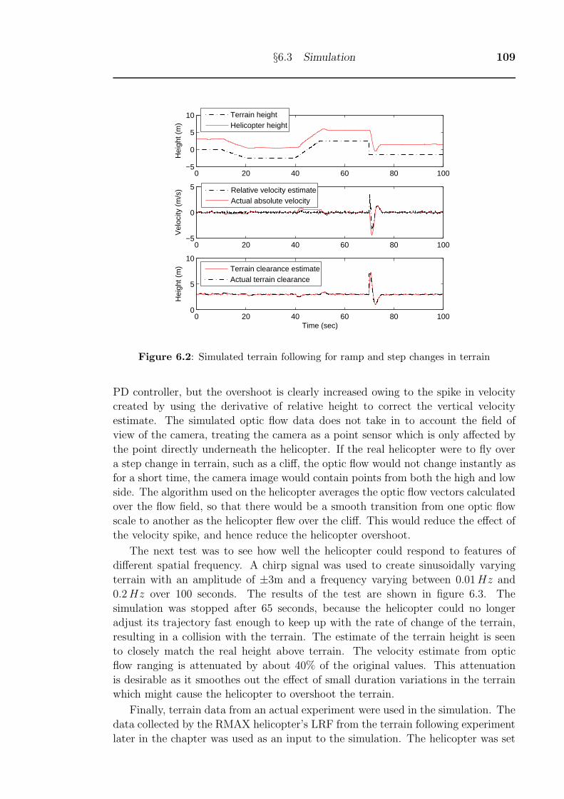
§6.3 Simulation 109
0 20 40 60 80 100−5
0
5
10
Hei
ght (
m)
Terrain heightHelicopter height
0 20 40 60 80 100−5
0
5V
eloc
ity (
m/s
) Relative velocity estimateActual absolute velocity
0 20 40 60 80 1000
5
10
Time (sec)
Hei
ght (
m) Terrain clearance estimate
Actual terrain clearance
Figure 6.2: Simulated terrain following for ramp and step changes in terrain
PD controller, but the overshoot is clearly increased owing to the spike in velocity
created by using the derivative of relative height to correct the vertical velocity
estimate. The simulated optic flow data does not take in to account the field of
view of the camera, treating the camera as a point sensor which is only affected by
the point directly underneath the helicopter. If the real helicopter were to fly over
a step change in terrain, such as a cliff, the optic flow would not change instantly as
for a short time, the camera image would contain points from both the high and low
side. The algorithm used on the helicopter averages the optic flow vectors calculated
over the flow field, so that there would be a smooth transition from one optic flow
scale to another as the helicopter flew over the cliff. This would reduce the effect of
the velocity spike, and hence reduce the helicopter overshoot.
The next test was to see how well the helicopter could respond to features of
different spatial frequency. A chirp signal was used to create sinusoidally varying
terrain with an amplitude of ±3m and a frequency varying between 0.01Hz and
0.2Hz over 100 seconds. The results of the test are shown in figure 6.3. The
simulation was stopped after 65 seconds, because the helicopter could no longer
adjust its trajectory fast enough to keep up with the rate of change of the terrain,
resulting in a collision with the terrain. The estimate of the terrain height is seen
to closely match the real height above terrain. The velocity estimate from optic
flow ranging is attenuated by about 40% of the original values. This attenuation
is desirable as it smoothes out the effect of small duration variations in the terrain
which might cause the helicopter to overshoot the terrain.
Finally, terrain data from an actual experiment were used in the simulation. The
data collected by the RMAX helicopter’s LRF from the terrain following experiment
later in the chapter was used as an input to the simulation. The helicopter was set
110 Control of Forward Flight
0 10 20 30 40 50 60 70−5
0
5
10H
eigh
t (m
)Terrain heightHelicopter height
0 10 20 30 40 50 60 70−5
0
5
Vel
ocity
(m
/s) Relative velocity estimate
Actual absolute velocity
0 10 20 30 40 50 60 700
2
4
6
Time (sec)
Hei
ght (
m)
Terrain clearance estimateActual terrain clearance
Figure 6.3: Simulated terrain following for sinusoidal terrain
to fly at the average speed of the RMAX during the test. The results are shown in
figure 6.4.
6.4 Terrain Following Experiments
6.4.1 Experimental Procedure
For the experimental work, a mechanism was required to allow the pilot to take over
control of the helicopter in event of a control or sensor failure. As the helicopter
quickly flies out of sight of the pilot in forward flight, a technique was used to chase
the helicopter at a relatively safe constant distance. The pilot was accomodated in
the back of a utility vehicle as shown in figure 6.5. The pilot crouched over the back
of the vehicle so that he had a clear view of the helicopter in flight. The driver of
the vehicle was instructed to maintain a constant distance from the helicopter.
6.4.2 Calculation of Optic Flow
For robustness, the optic flow calculation must be able to cope with flight at various
altitudes and speed. In forward flight, it must simultaneously measure small lateral
optic flow values whilst measuring large optic flows in the longitudinal direction.
When the optic flow shift exceeds the reference shift, the I2A ceases to function,
and its performance becomes unpredictable and degraded [71]. Ideally, reference
shifts would be choosen to be about double the expected optic flow so that there is
a sufficient margin over saturation whilst maintaining optimum measurement preci-
sion. Because of these considerations, an adaptive algorithm is required, otherwise
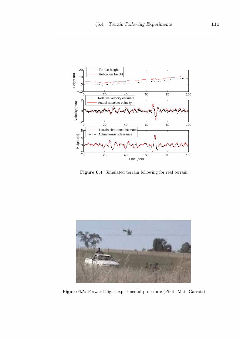
§6.4 Terrain Following Experiments 111
0 20 40 60 80 100−10
0
10
20H
eigh
t (m
)Terrain heightHelicopter height
0 20 40 60 80 100−2
0
2
Vel
ocity
(m
/s)
Relative velocity estimateActual absolute velocity
0 20 40 60 80 1002
3
4
5
Time (sec)
Hei
ght (
m)
Terrain clearance estimateActual terrain clearance
Figure 6.4: Simulated terrain following for real terrain
Figure 6.5: Forward flight experimental procedure (Pilot: Matt Garratt)

112 Control of Forward Flight
the optic flow measurement would be saturated at low altitude, too insensitive at
high altitude, and operable only in a very narrow range of height and speed.
To overcome the limited range of flow rates that can be measured using I2A, the
simple tracking estimator in Equation (6.7) was used to estimate the size of the next
image shift Sk+1 based on previous image shifts Sk and the measured optic flow Q.
The constant γ is a parameter between 0 and 1.0 adjusted to give stable tracking.
Sk+1 = γ (Sk +Q) + (1 − γ)Sk (6.7)
The expected shift is applied to the image before computation of optic flow, and
added to the result after computation, so that all measured shifts are less than 2
pixels. Despite the narrow range of the measurement, the adaptive feature of the
modified algorithm allows rates in excess of 10 pixels per frame to be measured
(over 700o/s with the camera used in the experiments). The adaptive version of the
I2A algorithm is known as the Iterative Image Interpolation Algorithm, abbreviated
I3A.
6.4.3 Terrain Following using Control by Telemetry
This test involved a control by telemetry scheme. All of the optic flow processing,
state estimation and control was executed on a real-time Linux PC in the chase
vehicle. A PC mounted in the chase vehicle was interfaced to the pilot’s transmitter
so that control could be switched between the pilot and the computer using a switch
on the transmitter.
The camera was oriented at 45o to the vertical axis of the helicopter to provide
some anticipation of terrain. For this test, DGPS information was not available.
As closed loop control of forward speed was not possible, the helicopter was instead
flown at a constant pitch attitude using a proportional feedback loop. The a priori
observed forward flight speed at this attitude was then used with Equation (6.1) to
provide a measurement of the height above ground using optic flow. Note that this
technique is only really applicable in low wind conditions as the open loop behaviour
of the helicopter can only be used to estimate air speed and not the ground speed
which is needed for accurate optic flow ranging. The height estimate was combined
with accelerometer information to provide an estimate of height and vertical velocity.
A PD controller was used to control collective pitch to maintain a datum height
of 2m above terrain. The pilot retained control of roll cyclic in order to keep the
helicopter on the desired ground track. Heading was controlled using a PID con-
troller.
The tests were performed on a flat, dry lake bed with the chase vehicle positioned
behind the helicopter. Before control was handed over to the computer system, the
helicopter was first established in forward flight under manual control. Once in
steady flight and telemetry confirmed, control was handed over to the computer.
After some initial tuning of gains, the helicopter was flown closed loop in a straight
line for over 2km with the optic flow ranging controlling height. The motion of the
helicopter was recorded by an external video camera but no provision was made for
recording the inertial data embedded in the telemetry stream. During the closed
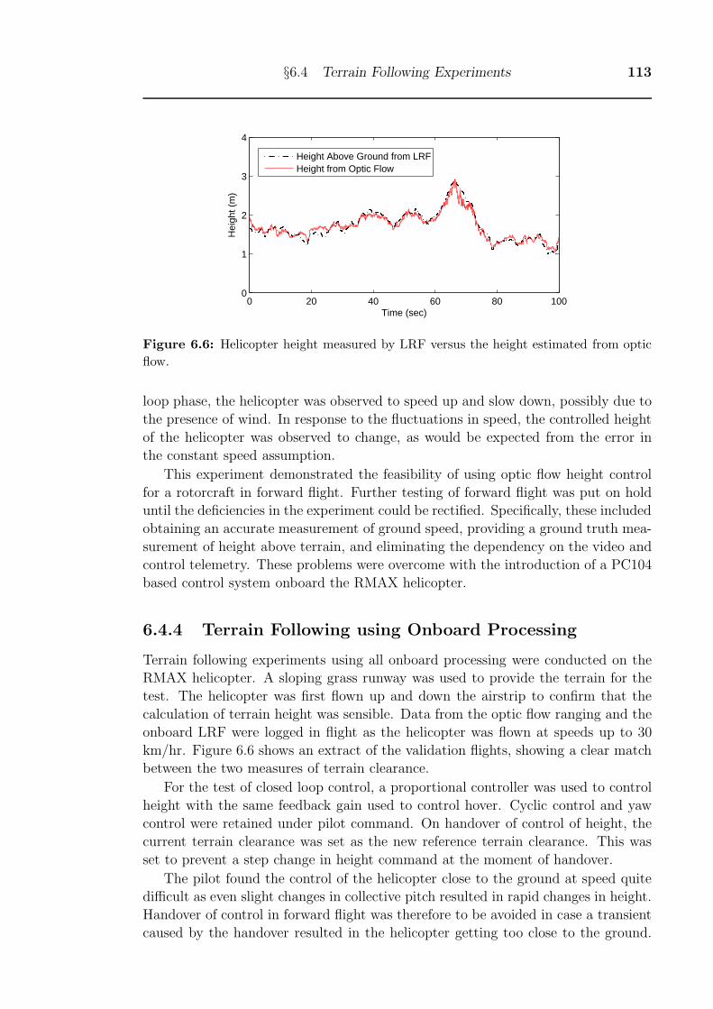
§6.4 Terrain Following Experiments 113
0 20 40 60 80 1000
1
2
3
4
Time (sec)
Hei
ght (
m)
Height Above Ground from LRFHeight from Optic Flow
Figure 6.6: Helicopter height measured by LRF versus the height estimated from optic
flow.
loop phase, the helicopter was observed to speed up and slow down, possibly due to
the presence of wind. In response to the fluctuations in speed, the controlled height
of the helicopter was observed to change, as would be expected from the error in
the constant speed assumption.
This experiment demonstrated the feasibility of using optic flow height control
for a rotorcraft in forward flight. Further testing of forward flight was put on hold
until the deficiencies in the experiment could be rectified. Specifically, these included
obtaining an accurate measurement of ground speed, providing a ground truth mea-
surement of height above terrain, and eliminating the dependency on the video and
control telemetry. These problems were overcome with the introduction of a PC104
based control system onboard the RMAX helicopter.
6.4.4 Terrain Following using Onboard Processing
Terrain following experiments using all onboard processing were conducted on the
RMAX helicopter. A sloping grass runway was used to provide the terrain for the
test. The helicopter was first flown up and down the airstrip to confirm that the
calculation of terrain height was sensible. Data from the optic flow ranging and the
onboard LRF were logged in flight as the helicopter was flown at speeds up to 30
km/hr. Figure 6.6 shows an extract of the validation flights, showing a clear match
between the two measures of terrain clearance.
For the test of closed loop control, a proportional controller was used to control
height with the same feedback gain used to control hover. Cyclic control and yaw
control were retained under pilot command. On handover of control of height, the
current terrain clearance was set as the new reference terrain clearance. This was
set to prevent a step change in height command at the moment of handover.
The pilot found the control of the helicopter close to the ground at speed quite
difficult as even slight changes in collective pitch resulted in rapid changes in height.
Handover of control in forward flight was therefore to be avoided in case a transient
caused by the handover resulted in the helicopter getting too close to the ground.
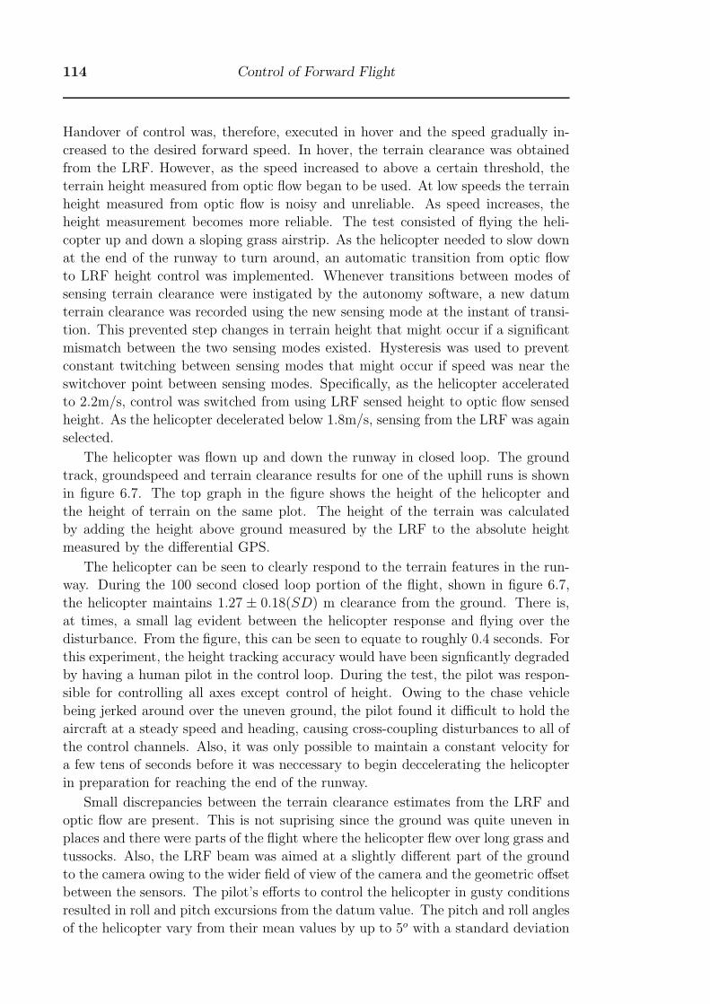
114 Control of Forward Flight
Handover of control was, therefore, executed in hover and the speed gradually in-
creased to the desired forward speed. In hover, the terrain clearance was obtained
from the LRF. However, as the speed increased to above a certain threshold, the
terrain height measured from optic flow began to be used. At low speeds the terrain
height measured from optic flow is noisy and unreliable. As speed increases, the
height measurement becomes more reliable. The test consisted of flying the heli-
copter up and down a sloping grass airstrip. As the helicopter needed to slow down
at the end of the runway to turn around, an automatic transition from optic flow
to LRF height control was implemented. Whenever transitions between modes of
sensing terrain clearance were instigated by the autonomy software, a new datum
terrain clearance was recorded using the new sensing mode at the instant of transi-
tion. This prevented step changes in terrain height that might occur if a significant
mismatch between the two sensing modes existed. Hysteresis was used to prevent
constant twitching between sensing modes that might occur if speed was near the
switchover point between sensing modes. Specifically, as the helicopter accelerated
to 2.2m/s, control was switched from using LRF sensed height to optic flow sensed
height. As the helicopter decelerated below 1.8m/s, sensing from the LRF was again
selected.
The helicopter was flown up and down the runway in closed loop. The ground
track, groundspeed and terrain clearance results for one of the uphill runs is shown
in figure 6.7. The top graph in the figure shows the height of the helicopter and
the height of terrain on the same plot. The height of the terrain was calculated
by adding the height above ground measured by the LRF to the absolute height
measured by the differential GPS.
The helicopter can be seen to clearly respond to the terrain features in the run-
way. During the 100 second closed loop portion of the flight, shown in figure 6.7,
the helicopter maintains 1.27 ± 0.18(SD) m clearance from the ground. There is,
at times, a small lag evident between the helicopter response and flying over the
disturbance. From the figure, this can be seen to equate to roughly 0.4 seconds. For
this experiment, the height tracking accuracy would have been signficantly degraded
by having a human pilot in the control loop. During the test, the pilot was respon-
sible for controlling all axes except control of height. Owing to the chase vehicle
being jerked around over the uneven ground, the pilot found it difficult to hold the
aircraft at a steady speed and heading, causing cross-coupling disturbances to all of
the control channels. Also, it was only possible to maintain a constant velocity for
a few tens of seconds before it was neccessary to begin deccelerating the helicopter
in preparation for reaching the end of the runway.
Small discrepancies between the terrain clearance estimates from the LRF and
optic flow are present. This is not suprising since the ground was quite uneven in
places and there were parts of the flight where the helicopter flew over long grass and
tussocks. Also, the LRF beam was aimed at a slightly different part of the ground
to the camera owing to the wider field of view of the camera and the geometric offset
between the sensors. The pilot’s efforts to control the helicopter in gusty conditions
resulted in roll and pitch excursions from the datum value. The pitch and roll angles
of the helicopter vary from their mean values by up to 5o with a standard deviation
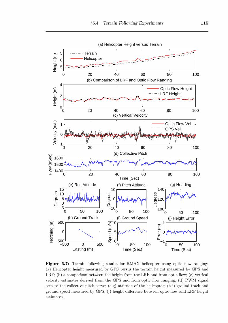
§6.4 Terrain Following Experiments 115
0 20 40 60 80 100
−5
0
5H
eigh
t (m
)
(a) Helicopter Height versus Terrain
TerrainHelicopter
0 20 40 60 80 1000
2
4
Hei
ght (
m)
(b) Comparison of LRF and Optic Flow Ranging
Optic Flow HeightLRF Height
0 20 40 60 80 100−1
0
1
Vel
ocity
(m
/s)
(c) Vertical Velocity
Optic Flow Vel.GPS Vel.
0 20 40 60 80 1001400
1500
1600
Time (Sec)
PW
M(u
Sec
) (d) Collective Pitch
0 50 100−5
05
1015
Deg
rees
(e) Roll Attitude
0 50 100−10
0
10
Deg
rees
(f) Pitch Attitude
0 50 100100
120
140
Deg
rees
(g) Heading
−500 0 500−500
0
500
Easting (m)
Nor
thin
g (m
)
(h) Ground Track
0 50 1000
5
10
Time (Sec)
Spe
ed (
m/s
)
(i) Ground Speed
0 50 100−1
0
1
Time (Sec)
Err
or (
m)
(j) Height Error
Figure 6.7: Terrain following results for RMAX helicopter using optic flow ranging:
(a) Helicopter height measured by GPS versus the terrain height measured by GPS and
LRF; (b) a comparison between the height from the LRF and from optic flow; (c) vertical
velocity estimates derived from the GPS and from optic flow ranging; (d) PWM signal
sent to the collective pitch servo; (e-g) attitude of the helicopter; (h-i) ground track and
ground speed measured by GPS; (j) height difference between optic flow and LRF height
estimates.
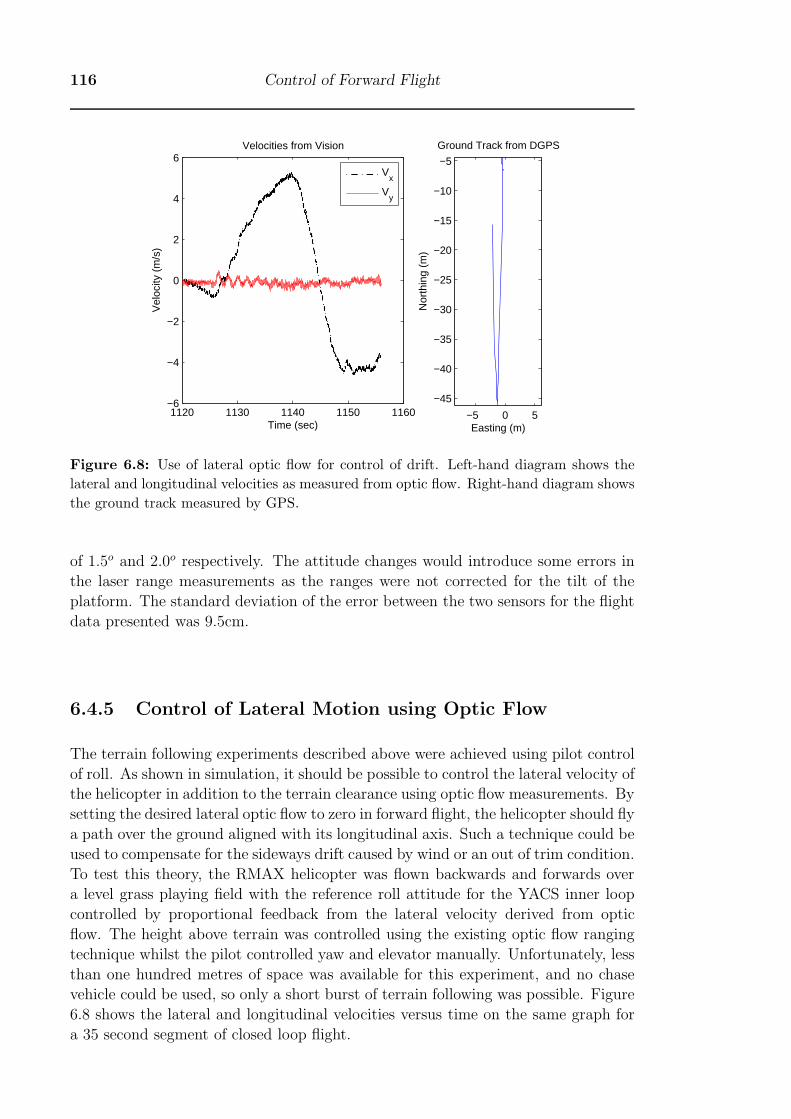
116 Control of Forward Flight
1120 1130 1140 1150 1160−6
−4
−2
0
2
4
6
Time (sec)
Vel
ocity
(m
/s)
Velocities from Vision
Vx
Vy
−5 0 5
−45
−40
−35
−30
−25
−20
−15
−10
−5
Easting (m)N
orth
ing
(m)
Ground Track from DGPS
Figure 6.8: Use of lateral optic flow for control of drift. Left-hand diagram shows the
lateral and longitudinal velocities as measured from optic flow. Right-hand diagram shows
the ground track measured by GPS.
of 1.5o and 2.0o respectively. The attitude changes would introduce some errors in
the laser range measurements as the ranges were not corrected for the tilt of the
platform. The standard deviation of the error between the two sensors for the flight
data presented was 9.5cm.
6.4.5 Control of Lateral Motion using Optic Flow
The terrain following experiments described above were achieved using pilot control
of roll. As shown in simulation, it should be possible to control the lateral velocity of
the helicopter in addition to the terrain clearance using optic flow measurements. By
setting the desired lateral optic flow to zero in forward flight, the helicopter should fly
a path over the ground aligned with its longitudinal axis. Such a technique could be
used to compensate for the sideways drift caused by wind or an out of trim condition.
To test this theory, the RMAX helicopter was flown backwards and forwards over
a level grass playing field with the reference roll attitude for the YACS inner loop
controlled by proportional feedback from the lateral velocity derived from optic
flow. The height above terrain was controlled using the existing optic flow ranging
technique whilst the pilot controlled yaw and elevator manually. Unfortunately, less
than one hundred metres of space was available for this experiment, and no chase
vehicle could be used, so only a short burst of terrain following was possible. Figure
6.8 shows the lateral and longitudinal velocities versus time on the same graph for
a 35 second segment of closed loop flight.
§6.5 Discussion 117
6.5 Discussion
The techniques presented in this chapter require an approximate measure of ground
speed. GPS velocity is one suitable means of velocity measurement. In the absence
of GPS, another measure of speed could be used such as airspeed from a pitot-
static air data system. However, airspeed needs to be corrected for the effect of
wind, otherwise the calculated range would have a scale error. Using airpseed would
result in a lower height above ground in a headwind and an increased height in a
tailwind.
The use of optic flow for height control is really most practical where an aircraft
is operating close to the ground. For example, a 747 cruising at Mach 0.86 and
40,000 feet generates an optic flow for a downwards looking camera of 1.5deg/sec.
Whilst this flow is certainly measurable, even a 1% error in ranging would result
in a 400ft error in height which would make it too inaccurate for traffic separation.
However, a 10% error in ranging for a terrain following aircraft flying at 400 ft would
be acceptable since this would generate an acceptable 40ft error, which is within the
existing error margin associated with flying over trees and uneven ground. The
scale, and hence accuracy, of the optic flow measurements could be optimised for
various applications by varying the frame rate. For a situation where the flow is
small, the frame rate could be reduced to increase the pixel shift and hence provide
a more easily measured signal. Digital processing hardware continues to increase in
speed, so it is concievable that it will soon, if not already, be possible to calculate
optic flow at several hundred frames per second, which would be fast enough for any
conceivable aircraft application.
As there is a lag between a change in terrain being sensed, and the response, some
a priori knowledge of the upcoming terrain could be used to improve performance.
The use of a downwards looking camera provides no anticipation of changes in
terrain ahead of the helicopter’s current position. By tilting the camera forward,
however, some anticipation of bumps could be applied. In [35], Hrabar proposes
that the optimum camera inclination for obstacle avoidance using optic flow is 45o.
This would introduce some inaccuracy in the range measurement if the simple range
equation (Eqn. (6.1)) was still used, since it assumes the camera axis is normal to
the ground. However, as the control by telemetry experiment demonstrated, the
method is sufficiently robust to cope with a 45o forward tilt of the camera without
any obvious side-effects, when using the average optic flow from the entire image.
In this work, the average optic flow over the whole image was used so that
the camera acts as a point sensor. In a more general situation, optic flow vectors
could be obtained and interpreted separately from different parts of the image. This
would provide not only the range, but also the azimuth and elevation of obstacles
that might be a threat to the vehicle. This would allow steering commands to
be generated in addition to height control. A limitation of this technique is that
objects in the direction of travel will not exhibit any translatory flow, so will not
be detected. Measurement of image expansion or loom could be used to detect
approaching obstacles at the front of an aircraft in forward flight, although this
signal tends to be weaker than the optic flow from motion parallel to a surface.
118 Control of Forward Flight
Future work should investigate the use of complete flow fields for obstacle avoidance.
6.6 Summary
In this section, systems for maintaining terrain clearance in an unstable rotorcraft
have been demonstrated and benchmarked against a LRF sensor. The system con-
sists of a downwards looking or forward tilted camera and computational hardware
to compute optic flow using the I3A algorithm. When combined with speed mea-
surements from GPS, the approach was able to estimate terrain clearance to within
7.5% of the actual mean height at an average forward flight speed of 20km/hr.
Lateral optic flow was also shown to be able to be used in forward flight to correct
sideways drift for a helicopter.
Chapter 7
Control using Artificial Neural
Networks
7.1 Introduction
In keeping with a biological inspiration for the system architecture, a neural network
based control system has been implemented. This technique has been applied to the
case of altitude control and the control of lateral and longitudinal drift in hover.
The aim of this chapter is to show that simple computational models can perform
the task of sensor fusion and control without a detailed mathematical model of
the plant being known. In biological systems, flight control and sensory processing
systems are partly hardwired into the animal as a result of evolutionary adaption
passed genetically and partly learnt from interaction with the environment. In this
case, off-line neural computational models will be trained using recorded data from
the real plant. Later work, beyond this thesis, could investigate the use of on-line
adaption to adapt the neural controllers to changing conditions and to improve the
control response.
Whilst we can use simplified mathematical models for designing controllers that
will work on the helicopter, there are many unmodelled dynamics that a simple
model will not incorporate. If we consider the collective control channel, for example,
significant errors can arise from ignoring or simplifying any of the following: actuator
kinematic non-linearities; ground effect; fuselage download; servo dynamics; rotor
speed variation; sensor lag; and rotor inflow lag associated with the rate of change
of collective pitch. These effects are virtually impossible to model exactly. The
use of ANNs does not require an explicit analytical model of these effects, only raw
flight test data from which a black-box model can be learnt. This simplifies the
controller design significantly and allows the ANN controllers to be run on very
simple hardware.
The 7 state EKF prediction and correction cycle used for fusing inertial and visual
information discussed in Chapter 8 executes on PC104 hardware in approximately
1ms. By comparison, a single layer feedforward ANN with eight hidden nodes used
to fuse inertials and vision executes in about 10μs on the same hardware. An
ANN can be executed on much simpler processors than an EKF and may have
other advantages in terms of robustness to unforeseen variations in sensor noise
characteristics.
119
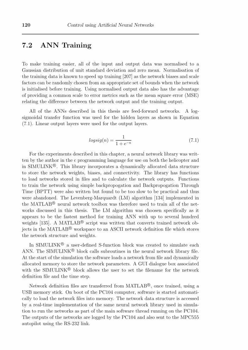
120 Control using Artificial Neural Networks
7.2 ANN Training
To make training easier, all of the input and output data was normalised to a
Gaussian distribution of unit standard deviation and zero mean. Normalisation of
the training data is known to speed up training [207] as the network biases and scale
factors can be randomly chosen from an appropriate set of bounds when the network
is initialised before training. Using normalised output data also has the advantage
of providing a common scale to error metrics such as the mean square error (MSE)
relating the difference between the network output and the training output.
All of the ANNs described in this thesis are feed-forward networks. A log-
sigmoidal transfer function was used for the hidden layers as shown in Equation
(7.1). Linear output layers were used for the output layers.
logsig(n) =1
1 + e−n(7.1)
For the experiments described in this chapter, a neural network library was writ-
ten by the author in the c programming language for use on both the helicopter and
in SIMULINKR©. This library incorporates a dynamically allocated data structure
to store the network weights, biases, and connectivity. The library has functions
to load networks stored in files and to calculate the network outputs. Functions
to train the network using simple backpropogation and Backpropogation Through
Time (BPTT) were also written but found to be too slow to be practical and thus
were abandoned. The Levenberg-Marquardt (LM) algorithm [134] implemented in
the MATLABR© neural network toolbox was therefore used to train all of the net-
works discussed in this thesis. The LM algorithm was choosen specifically as it
appears to be the fastest method for training ANN with up to several hundred
weights [135]. A MATLABR© script was written that converts trained network ob-
jects in the MATLABR© workspace to an ASCII network definition file which stores
the network structure and weights.
In SIMULINK R© a user-defined S-function block was created to simulate each
ANN. The SIMULINK R© block calls subroutines in the neural network library file.
At the start of the simulation the software loads a network from file and dynamically
allocated memory to store the network parameters. A GUI dialogue box associated
with the SIMULINKR© block allows the user to set the filename for the network
definition file and the time step.
Network definition files are transferred from MATLABR©, once trained, using a
USB memory stick. On boot of the PC104 computer, software is started automati-
cally to load the network files into memory. The network data structure is accessed
by a real-time implementation of the same neural network library used in simula-
tion to run the networks as part of the main software thread running on the PC104.
The outputs of the networks are logged by the PC104 and also sent to the MPC555
autopilot using the RS-232 link.
§7.3 Control of Height using a Neural Network 121
7.3 Control of Height using a Neural Network
In this section, the control of height using a neural network is first shown to be
feasible using a simplified simulation of the helicopter dynamics. The approach is
then shown to work on the real helicopter based on a plant model trained from real
flight data. For this thesis, the helicopter height has been measured by a number
of means including using a stereo camera, height from optic flow (only in forward
flight), laser range finding and DGPS. For the work in this chapter, which was
carried out on the Eagle helicopter, only DGPS height will be used, however the
methods apply equally well to any of the other sensing modes.
The strategy used for control of height is a three-step process aiming at achieving
an ANN implementation of an optimal controller. The process consists of training a
neural network to represent the plant, developing a controller off-line using compu-
tationally intensive, but optimal methods, and then training another neural network
to mimic the optimal controller. The technique has a number of advantages. Firstly,
an optimal controller can be designed and tested in simulation using full and noise-
free state data which may not be available in flight. The ANN can be trained to
mimic the optimal controller but using only the data which it has available to it,
which may be uncalibrated, corrupted by noise and affected by sensor lag. For
example, the optimal controller might be executed with noise-free vertical velocity
and height data but the ANN may only be given height data with no velocity infor-
mation. Secondly, the optimisation process is computationally intensive and could
not be achieved in real-time. The use of optimal control is of particular interest in
this work, as biological entities will have optimised their control pathways through
evolutionary process and also learned behavior during their individual lifetimes.
In order to develop an optimal controller for the helicopter, a means of captur-
ing the dynamics of the helicopter is required. Certain aspects of the dynamics are
known exactly. For example it is known from basic physics that the vertical accel-
eration can be integrated exactly to obtain vertical velocity and integrated again to
obtain height. Furthermore, the dynamics of the collective servo have been measured
directly and can be hard wired in to a model of the plant. The remaining dynamics
involve the relationship between the vertical acceleration and the collective pitch,
vertical velocity and ground effect. This relationship is affected by the kinematic
relationship between the servo input and the blade pitch, the vertical drag on the
fuselage caused by the downwash and rate of climb/descent and other effects. These
non-linear dynamics are more difficult to predict analytically and would require a
tedious experimental effort to model accurately. An ANN is therefore one means
of capturing this dynamic behavior in one step without a detailed mathematical
model.
The helicopter is fitted with a vertical accelerometer which allows the vertical
acceleration to be recorded from flight test and used to train the ANN plant model.
The accelerometer measures the local acceleration which is the sum of the component
of gravitational acceleration (g) and the rate of change of velocity of the platform.
The z-accelerometer output az is actually just equal to the net aerodynamic z-
axis force (T) acting on the helicopter divided by the helicopter mass (m), so that
122 Control using Artificial Neural Networks
az = T/M . The force T is the net effect of the main rotor thrust and the vertical drag
caused by the rotor downwash. No compensation for pitch and roll tilt is required as
the accelerometer moves with the helicopter local axes. Although counter-intuitive
this can be understood by considering a simple helicopter of mass (m) with no tail
rotor side force so that it hovers perfectly level with thrust (T) equal to weight
(W). If the helicopter is in equilibrium hover, T = W and the accelerometer would
measure az = W/m = T/m. If the thrust of the helicopter suddenly changed to zero,
the helicopter would be in free-fall and the accelerometer would be zero, so that still
az = T/m = 0. If the helicopter suddenly rolls to 45◦ without changing its thrust,
the helicopter would begin to fly sideways and descend since the vertical component
of thrust is now less than the weight force. The accelerometer would measure the
sum of the z-axis component of gravity and the rate of change of z-axis velocity
which is −gcos45◦ + (mg cos 45◦ − T )/m = T/m. In each case, the accelerometer
still measures T/M regardless of the effect of gravity and tilt. The significance
of this is that all of the aerodynamic effects are encapsulated in the measurement
of az, so that training a neural network to represent az is the same as training a
neural network to represent the aerodynamics of vertical flight. The dynamics of the
vehicle, which is essentially integrating the acceleration to get velocity and position,
are known exactly and for these purposes do not need to be represented by an ANN
as they are very simply implemented. However, if desired, use of a recurrent neural
network would allow the integration of acceleration to be carried out by the ANN
also.
7.3.1 Simulation of Height Control using an ANN
The feasibility of using an ANN to control height was first tested in simulation
using SIMULINK R©. The first objective was to train a neural network to mimic
an analytical model of the helicopter and then see if this ANN could be used to
develop an optimal controller to control the plant. The second objective was to see
if another ANN could then be trained to mimic the optimal plant and to see how
well this ANN could do the job of the optimal controller.
The vertical dynamic components of the eagle simulation developed in Chapter
3 were isolated to generate simulated helicopter data. The rotor induced flow model
calculates thrust given collective pitch and vertical velocity as inputs. The weight
of the helicopter is subtracted from the thrust and divided by mass to calculate the
vertical acceleration. This acceleration is then integrated twice to get the velocity
and height. For the purposes of this test, ground effect was not included in the
vertical flight model. A servo model based on the measured dynamics was however
included.
The objective of the simulation is to provide training data to allow an ANN to
be trained to mimic the plant. A large training set was desired to adequately span
the possible combinations of vertical velocity and collective pitch. The plant model
was stimulated to provide this training set using a random step block in series with
a rate limiter to generate a reference set of desired vertical velocities to drive the
model. The random step block was set to output velocities using a step period
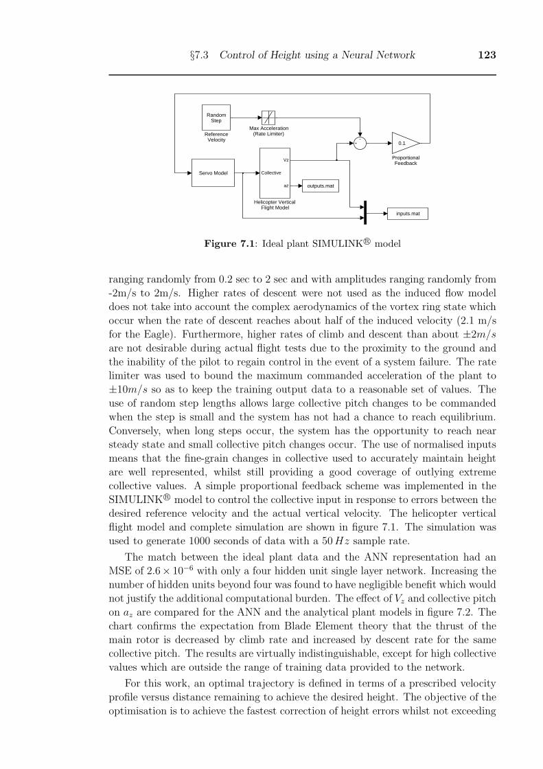
§7.3 Control of Height using a Neural Network 123
inputs.mat
outputs.mat
Servo Model
RandomStep
ReferenceVelocity
0.1
ProportionalFeedback
Max Acceleration(Rate Limiter)
Collective
Vz
az
Helicopter Vertical Flight Model
Figure 7.1: Ideal plant SIMULINK R© model
ranging randomly from 0.2 sec to 2 sec and with amplitudes ranging randomly from
-2m/s to 2m/s. Higher rates of descent were not used as the induced flow model
does not take into account the complex aerodynamics of the vortex ring state which
occur when the rate of descent reaches about half of the induced velocity (2.1 m/s
for the Eagle). Furthermore, higher rates of climb and descent than about ±2m/s
are not desirable during actual flight tests due to the proximity to the ground and
the inability of the pilot to regain control in the event of a system failure. The rate
limiter was used to bound the maximum commanded acceleration of the plant to
±10m/s so as to keep the training output data to a reasonable set of values. The
use of random step lengths allows large collective pitch changes to be commanded
when the step is small and the system has not had a chance to reach equilibrium.
Conversely, when long steps occur, the system has the opportunity to reach near
steady state and small collective pitch changes occur. The use of normalised inputs
means that the fine-grain changes in collective used to accurately maintain height
are well represented, whilst still providing a good coverage of outlying extreme
collective values. A simple proportional feedback scheme was implemented in the
SIMULINK R© model to control the collective input in response to errors between the
desired reference velocity and the actual vertical velocity. The helicopter vertical
flight model and complete simulation are shown in figure 7.1. The simulation was
used to generate 1000 seconds of data with a 50Hz sample rate.
The match between the ideal plant data and the ANN representation had an
MSE of 2.6× 10⁻⁶ with only a four hidden unit single layer network. Increasing the
number of hidden units beyond four was found to have negligible benefit which would
not justify the additional computational burden. The effect of Vz and collective pitch
on az are compared for the ANN and the analytical plant models in figure 7.2. The
chart confirms the expectation from Blade Element theory that the thrust of the
main rotor is decreased by climb rate and increased by descent rate for the same
collective pitch. The results are virtually indistinguishable, except for high collective
values which are outside the range of training data provided to the network.
For this work, an optimal trajectory is defined in terms of a prescribed velocity
profile versus distance remaining to achieve the desired height. The objective of the
optimisation is to achieve the fastest correction of height errors whilst not exceeding
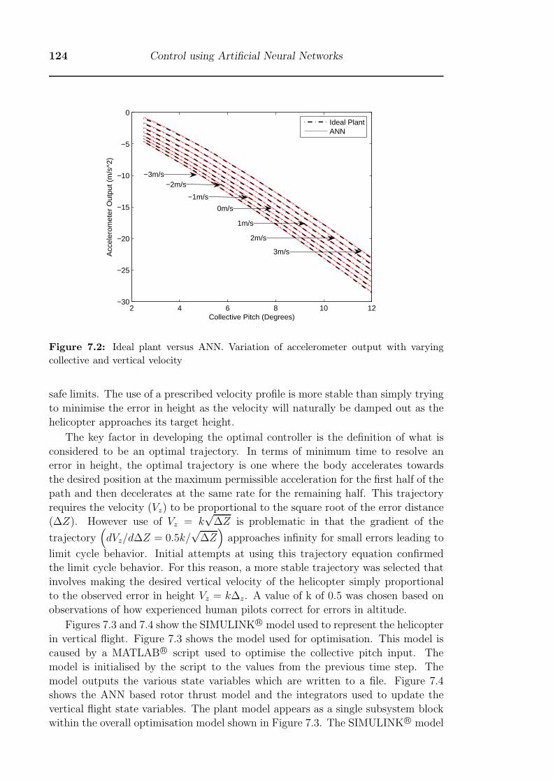
124 Control using Artificial Neural Networks
2 4 6 8 10 12−30
−25
−20
−15
−10
−5
0
Collective Pitch (Degrees)
Acc
eler
omet
er O
utpu
t (m
/s^2
)
Ideal PlantANN
−3m/s−2m/s
−1m/s
0m/s
1m/s
2m/s
3m/s
Figure 7.2: Ideal plant versus ANN. Variation of accelerometer output with varying
collective and vertical velocity
safe limits. The use of a prescribed velocity profile is more stable than simply trying
to minimise the error in height as the velocity will naturally be damped out as the
helicopter approaches its target height.
The key factor in developing the optimal controller is the definition of what is
considered to be an optimal trajectory. In terms of minimum time to resolve an
error in height, the optimal trajectory is one where the body accelerates towards
the desired position at the maximum permissible acceleration for the first half of the
path and then decelerates at the same rate for the remaining half. This trajectory
requires the velocity (Vz) to be proportional to the square root of the error distance
(ΔZ). However use of Vz = k√
ΔZ is problematic in that the gradient of the
trajectory(dVz/dΔZ = 0.5k/
√ΔZ)
approaches infinity for small errors leading to
limit cycle behavior. Initial attempts at using this trajectory equation confirmed
the limit cycle behavior. For this reason, a more stable trajectory was selected that
involves making the desired vertical velocity of the helicopter simply proportional
to the observed error in height Vz = kΔz. A value of k of 0.5 was chosen based on
observations of how experienced human pilots correct for errors in altitude.
Figures 7.3 and 7.4 show the SIMULINKR© model used to represent the helicopter
in vertical flight. Figure 7.3 shows the model used for optimisation. This model is
caused by a MATLABR© script used to optimise the collective pitch input. The
model is initialised by the script to the values from the previous time step. The
model outputs the various state variables which are written to a file. Figure 7.4
shows the ANN based rotor thrust model and the integrators used to update the
vertical flight state variables. The plant model appears as a single subsystem block
within the overall optimisation model shown in Figure 7.3. The SIMULINKR© model
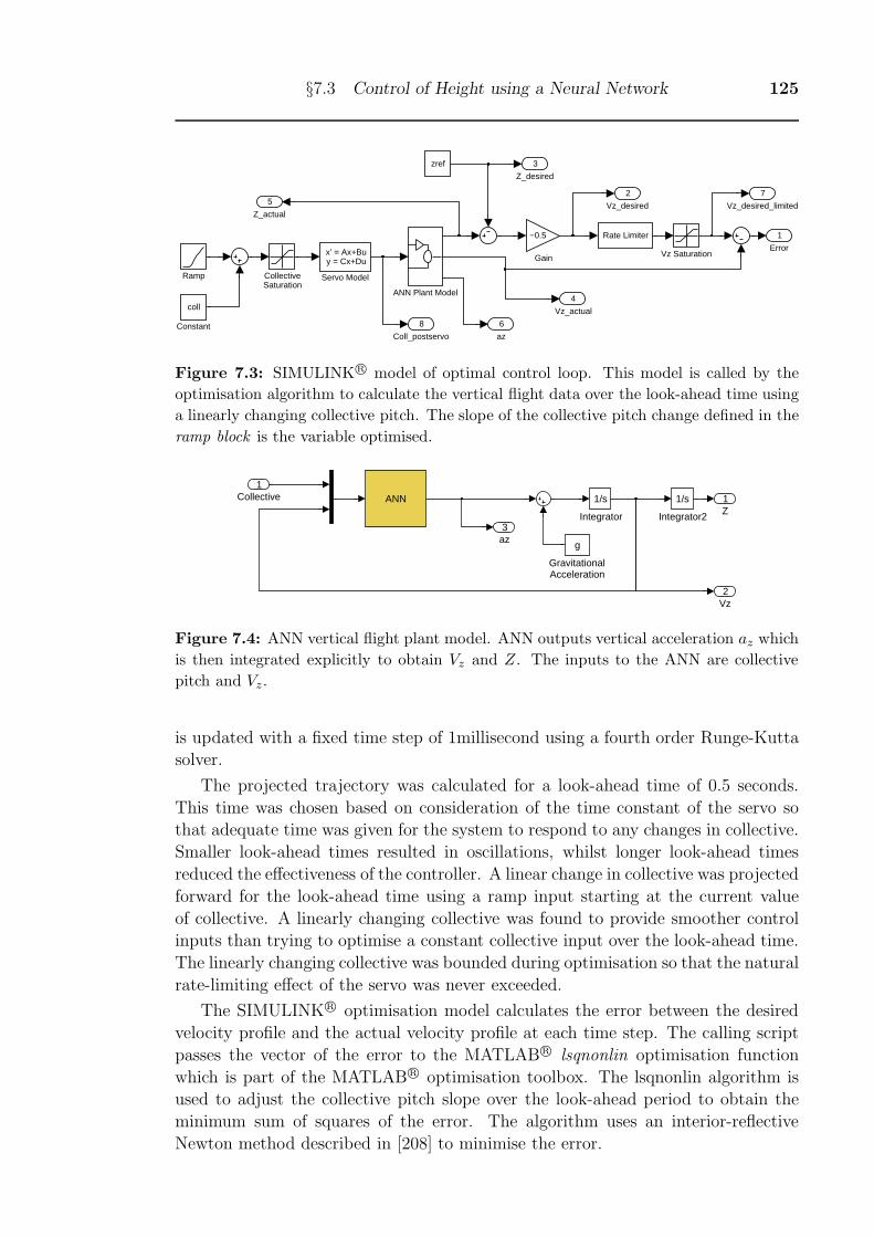
§7.3 Control of Height using a Neural Network 125
8
Coll_postservo
7
Vz_desired_limited
6
az
5
Z_actual
4
Vz_actual
3
Z_desired
2
Vz_desired
1
Error
zref
Vz Saturationx’ = Ax+Bu y = Cx+Du
Servo Model
Rate Limiter
Ramp
−0.5
Gain
coll
Constant
CollectiveSaturation
ANN Plant Model
Figure 7.3: SIMULINK R© model of optimal control loop. This model is called by the
optimisation algorithm to calculate the vertical flight data over the look-ahead time using
a linearly changing collective pitch. The slope of the collective pitch change defined in the
ramp block is the variable optimised.
3az
2Vz
1Z
ANN 1/s
Integrator2
1/s
Integrator
g
GravitationalAcceleration
1Collective
Figure 7.4: ANN vertical flight plant model. ANN outputs vertical acceleration az which
is then integrated explicitly to obtain Vz and Z. The inputs to the ANN are collective
pitch and Vz.
is updated with a fixed time step of 1millisecond using a fourth order Runge-Kutta
solver.
The projected trajectory was calculated for a look-ahead time of 0.5 seconds.
This time was chosen based on consideration of the time constant of the servo so
that adequate time was given for the system to respond to any changes in collective.
Smaller look-ahead times resulted in oscillations, whilst longer look-ahead times
reduced the effectiveness of the controller. A linear change in collective was projected
forward for the look-ahead time using a ramp input starting at the current value
of collective. A linearly changing collective was found to provide smoother control
inputs than trying to optimise a constant collective input over the look-ahead time.
The linearly changing collective was bounded during optimisation so that the natural
rate-limiting effect of the servo was never exceeded.
The SIMULINK R© optimisation model calculates the error between the desired
velocity profile and the actual velocity profile at each time step. The calling script
passes the vector of the error to the MATLABR© lsqnonlin optimisation function
which is part of the MATLABR© optimisation toolbox. The lsqnonlin algorithm is
used to adjust the collective pitch slope over the look-ahead period to obtain the
minimum sum of squares of the error. The algorithm uses an interior-reflective
Newton method described in [208] to minimise the error.
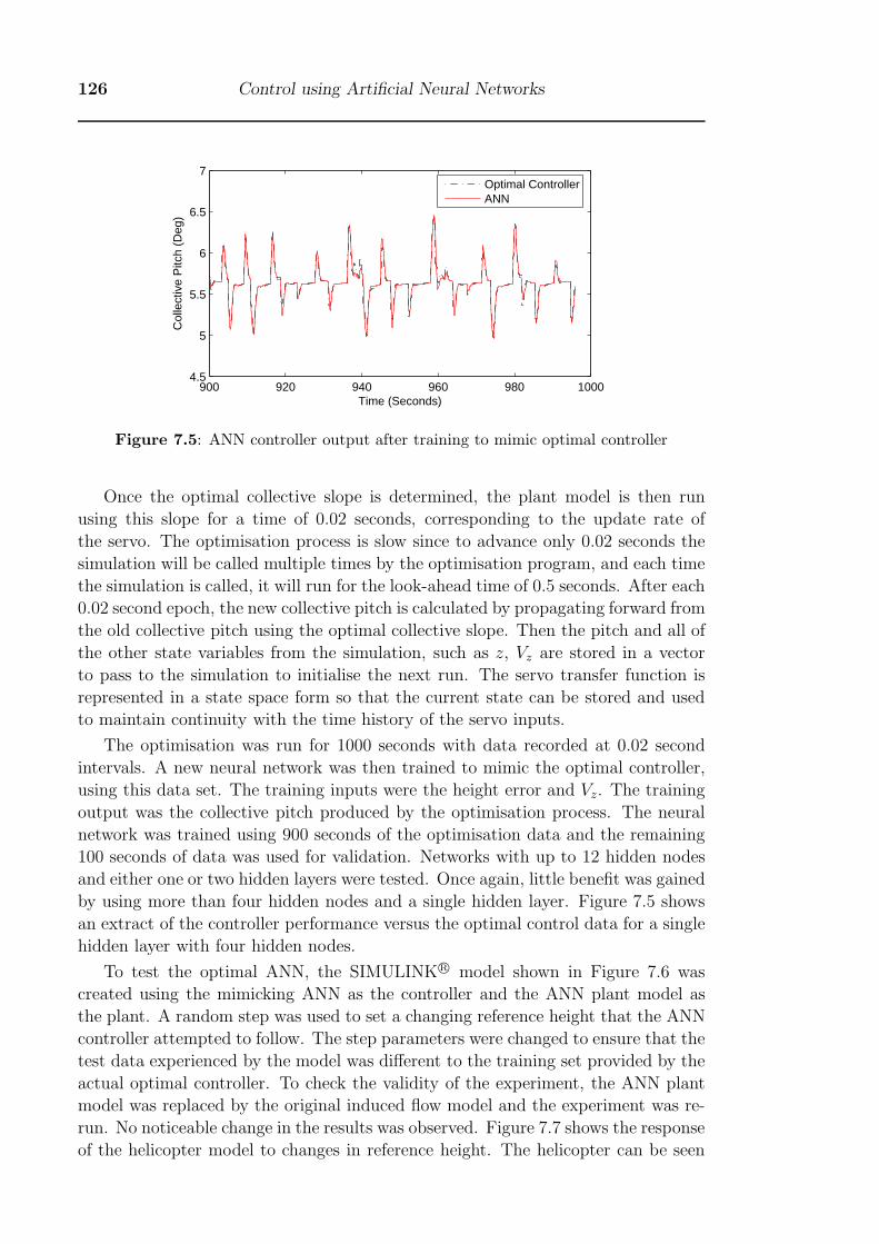
126 Control using Artificial Neural Networks
900 920 940 960 980 10004.5
5
5.5
6
6.5
7
Time (Seconds)
Col
lect
ive
Pitc
h (D
eg)
Optimal ControllerANN
Figure 7.5: ANN controller output after training to mimic optimal controller
Once the optimal collective slope is determined, the plant model is then run
using this slope for a time of 0.02 seconds, corresponding to the update rate of
the servo. The optimisation process is slow since to advance only 0.02 seconds the
simulation will be called multiple times by the optimisation program, and each time
the simulation is called, it will run for the look-ahead time of 0.5 seconds. After each
0.02 second epoch, the new collective pitch is calculated by propagating forward from
the old collective pitch using the optimal collective slope. Then the pitch and all of
the other state variables from the simulation, such as z, Vz are stored in a vector
to pass to the simulation to initialise the next run. The servo transfer function is
represented in a state space form so that the current state can be stored and used
to maintain continuity with the time history of the servo inputs.
The optimisation was run for 1000 seconds with data recorded at 0.02 second
intervals. A new neural network was then trained to mimic the optimal controller,
using this data set. The training inputs were the height error and Vz. The training
output was the collective pitch produced by the optimisation process. The neural
network was trained using 900 seconds of the optimisation data and the remaining
100 seconds of data was used for validation. Networks with up to 12 hidden nodes
and either one or two hidden layers were tested. Once again, little benefit was gained
by using more than four hidden nodes and a single hidden layer. Figure 7.5 shows
an extract of the controller performance versus the optimal control data for a single
hidden layer with four hidden nodes.
To test the optimal ANN, the SIMULINKR© model shown in Figure 7.6 was
created using the mimicking ANN as the controller and the ANN plant model as
the plant. A random step was used to set a changing reference height that the ANN
controller attempted to follow. The step parameters were changed to ensure that the
test data experienced by the model was different to the training set provided by the
actual optimal controller. To check the validity of the experiment, the ANN plant
model was replaced by the original induced flow model and the experiment was re-
run. No noticeable change in the results was observed. Figure 7.7 shows the response
of the helicopter model to changes in reference height. The helicopter can be seen
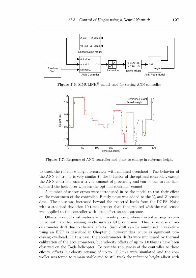
§7.3 Control of Height using a Neural Network 127
RandomStep
x’ = Ax+Bu y = Cx+Du
Servo Model
Z_clean
Vz_Clean
Z_out
Vz_out
Sensor/Noise Model
Saturation
Coll
Vz
Height
ANN Plant Model
Actual Vz
Actual Z
Desired Z
Coll
ANN Controller
Figure 7.6: SIMULINK R© model used for testing ANN controller
0 50 100 150 200 250 300−2
−1.5
−1
−0.5
0
0.5
1
1.5
2
Time (Seconds)
Hei
ght (
m)
Reference HeightActual Height
Figure 7.7: Response of ANN controller and plant to change in reference height
to track the reference height accurately with minimal overshoot. The behavior of
the ANN controller is very similar to the behavior of the optimal controller, except
the ANN controller uses a trivial amount of processing and can be run in real-time
onboard the helicopter whereas the optimal controller cannot.
A number of sensor errors were introduced in to the model to test their effect
on the robustness of the controller. Firstly noise was added to the Vz and Z sensor
data. The noise was increased beyond the expected levels from the DGPS. Noise
with a standard deviation 10 times greater than that realised with the real sensor
was applied to the controller with little effect on the outcome.
Offsets in velocity estimates are commonly present where inertial sensing is com-
bined with another sensing mode such as GPS or vision. This is because of ac-
celerometer drift due to thermal effects. Such drift can be minimised in real-time
using an EKF as described in Chapter 8, however this incurs as significant pro-
cessing overhead. In this case, the accelerometer drifts were minimised by thermal
calibration of the accelerometers, but velocity offsets of up to ±0.05m/s have been
observed on the Eagle helicopter. To test the robustness of the controller to these
effects, offsets in velocity sensing of up to ±0.2m/s were simulated and the con-
troller was found to remain stable and to still track the reference height albeit with
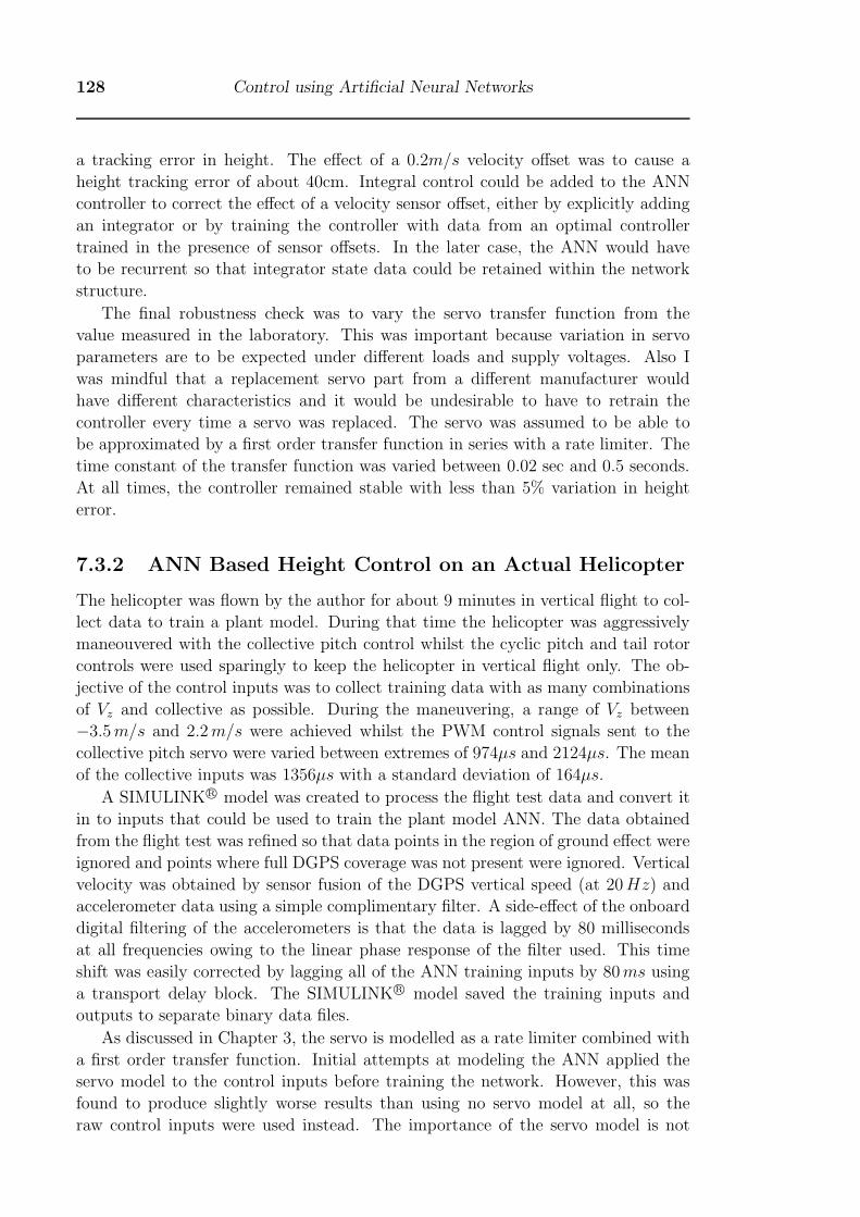
128 Control using Artificial Neural Networks
a tracking error in height. The effect of a 0.2m/s velocity offset was to cause a
height tracking error of about 40cm. Integral control could be added to the ANN
controller to correct the effect of a velocity sensor offset, either by explicitly adding
an integrator or by training the controller with data from an optimal controller
trained in the presence of sensor offsets. In the later case, the ANN would have
to be recurrent so that integrator state data could be retained within the network
structure.
The final robustness check was to vary the servo transfer function from the
value measured in the laboratory. This was important because variation in servo
parameters are to be expected under different loads and supply voltages. Also I
was mindful that a replacement servo part from a different manufacturer would
have different characteristics and it would be undesirable to have to retrain the
controller every time a servo was replaced. The servo was assumed to be able to
be approximated by a first order transfer function in series with a rate limiter. The
time constant of the transfer function was varied between 0.02 sec and 0.5 seconds.
At all times, the controller remained stable with less than 5% variation in height
error.
7.3.2 ANN Based Height Control on an Actual Helicopter
The helicopter was flown by the author for about 9 minutes in vertical flight to col-
lect data to train a plant model. During that time the helicopter was aggressively
maneouvered with the collective pitch control whilst the cyclic pitch and tail rotor
controls were used sparingly to keep the helicopter in vertical flight only. The ob-
jective of the control inputs was to collect training data with as many combinations
of Vz and collective as possible. During the maneuvering, a range of Vz between
−3.5m/s and 2.2m/s were achieved whilst the PWM control signals sent to the
collective pitch servo were varied between extremes of 974μs and 2124μs. The mean
of the collective inputs was 1356μs with a standard deviation of 164μs.
A SIMULINK R© model was created to process the flight test data and convert it
in to inputs that could be used to train the plant model ANN. The data obtained
from the flight test was refined so that data points in the region of ground effect were
ignored and points where full DGPS coverage was not present were ignored. Vertical
velocity was obtained by sensor fusion of the DGPS vertical speed (at 20Hz) and
accelerometer data using a simple complimentary filter. A side-effect of the onboard
digital filtering of the accelerometers is that the data is lagged by 80 milliseconds
at all frequencies owing to the linear phase response of the filter used. This time
shift was easily corrected by lagging all of the ANN training inputs by 80ms using
a transport delay block. The SIMULINKR© model saved the training inputs and
outputs to separate binary data files.
As discussed in Chapter 3, the servo is modelled as a rate limiter combined with
a first order transfer function. Initial attempts at modeling the ANN applied the
servo model to the control inputs before training the network. However, this was
found to produce slightly worse results than using no servo model at all, so the
raw control inputs were used instead. The importance of the servo model is not
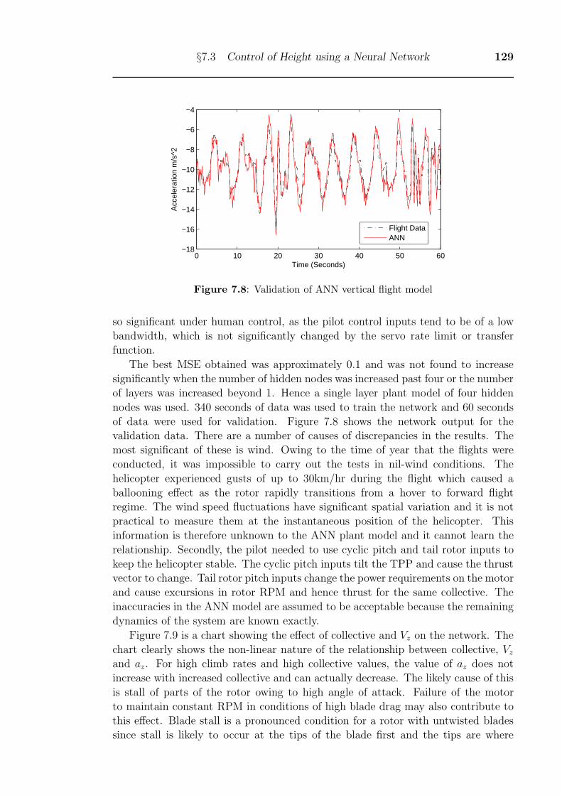
§7.3 Control of Height using a Neural Network 129
0 10 20 30 40 50 60−18
−16
−14
−12
−10
−8
−6
−4
Time (Seconds)
Acc
eler
atio
n m
/s^2
Flight DataANN
Figure 7.8: Validation of ANN vertical flight model
so significant under human control, as the pilot control inputs tend to be of a low
bandwidth, which is not significantly changed by the servo rate limit or transfer
function.
The best MSE obtained was approximately 0.1 and was not found to increase
significantly when the number of hidden nodes was increased past four or the number
of layers was increased beyond 1. Hence a single layer plant model of four hidden
nodes was used. 340 seconds of data was used to train the network and 60 seconds
of data were used for validation. Figure 7.8 shows the network output for the
validation data. There are a number of causes of discrepancies in the results. The
most significant of these is wind. Owing to the time of year that the flights were
conducted, it was impossible to carry out the tests in nil-wind conditions. The
helicopter experienced gusts of up to 30km/hr during the flight which caused a
ballooning effect as the rotor rapidly transitions from a hover to forward flight
regime. The wind speed fluctuations have significant spatial variation and it is not
practical to measure them at the instantaneous position of the helicopter. This
information is therefore unknown to the ANN plant model and it cannot learn the
relationship. Secondly, the pilot needed to use cyclic pitch and tail rotor inputs to
keep the helicopter stable. The cyclic pitch inputs tilt the TPP and cause the thrust
vector to change. Tail rotor pitch inputs change the power requirements on the motor
and cause excursions in rotor RPM and hence thrust for the same collective. The
inaccuracies in the ANN model are assumed to be acceptable because the remaining
dynamics of the system are known exactly.
Figure 7.9 is a chart showing the effect of collective and Vz on the network. The
chart clearly shows the non-linear nature of the relationship between collective, Vzand az. For high climb rates and high collective values, the value of az does not
increase with increased collective and can actually decrease. The likely cause of this
is stall of parts of the rotor owing to high angle of attack. Failure of the motor
to maintain constant RPM in conditions of high blade drag may also contribute to
this effect. Blade stall is a pronounced condition for a rotor with untwisted blades
since stall is likely to occur at the tips of the blade first and the tips are where
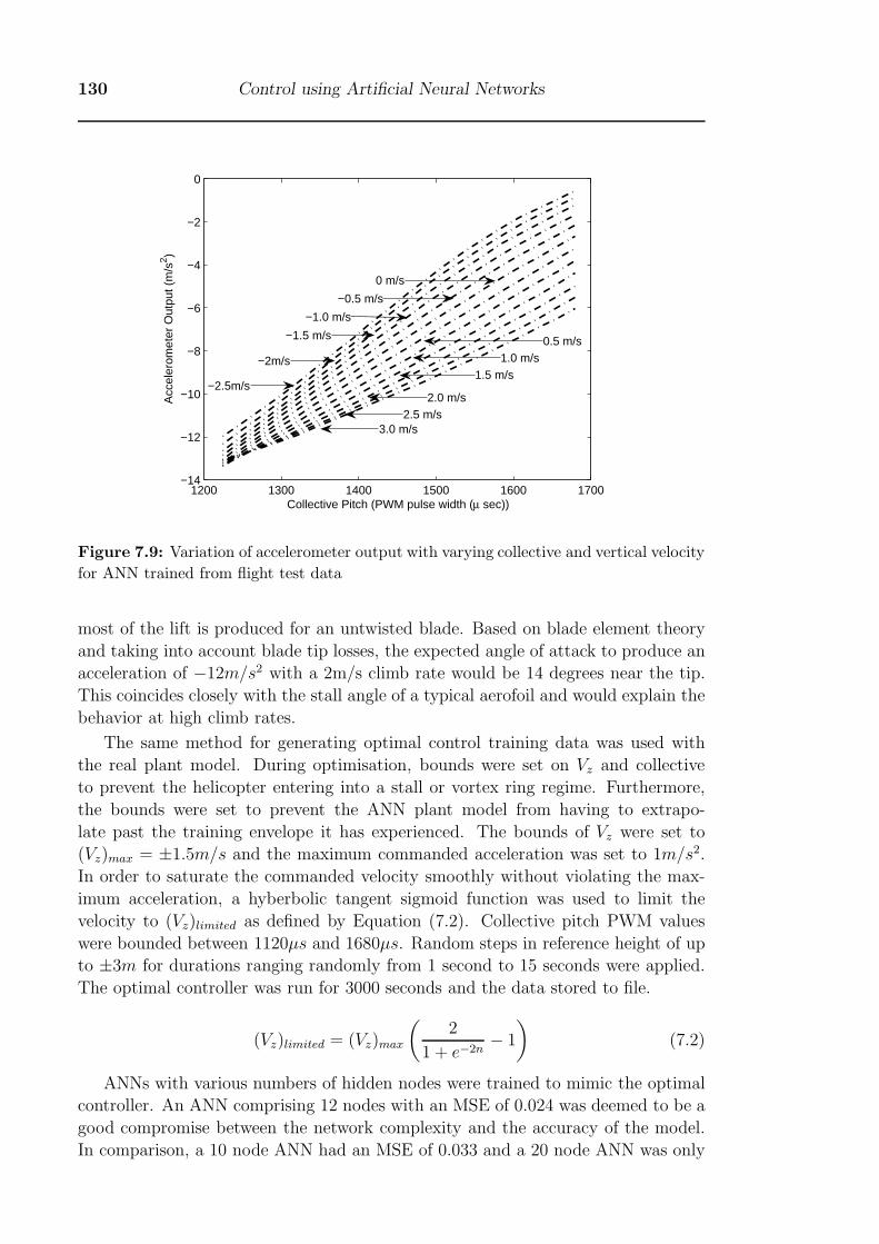
130 Control using Artificial Neural Networks
1200 1300 1400 1500 1600 1700−14
−12
−10
−8
−6
−4
−2
0
Collective Pitch (PWM pulse width (μ sec))
Acc
eler
omet
er O
utpu
t (m
/s2 )
0 m/s
−0.5 m/s
−1.5 m/s
−1.0 m/s
0.5 m/s1.0 m/s
3.0 m/s
−2m/s
2.5 m/s
1.5 m/s
2.0 m/s−2.5m/s
Figure 7.9: Variation of accelerometer output with varying collective and vertical velocity
for ANN trained from flight test data
most of the lift is produced for an untwisted blade. Based on blade element theory
and taking into account blade tip losses, the expected angle of attack to produce an
acceleration of −12m/s2 with a 2m/s climb rate would be 14 degrees near the tip.
This coincides closely with the stall angle of a typical aerofoil and would explain the
behavior at high climb rates.
The same method for generating optimal control training data was used with
the real plant model. During optimisation, bounds were set on Vz and collective
to prevent the helicopter entering into a stall or vortex ring regime. Furthermore,
the bounds were set to prevent the ANN plant model from having to extrapo-
late past the training envelope it has experienced. The bounds of Vz were set to
(Vz)max = ±1.5m/s and the maximum commanded acceleration was set to 1m/s2.
In order to saturate the commanded velocity smoothly without violating the max-
imum acceleration, a hyberbolic tangent sigmoid function was used to limit the
velocity to (Vz)limited as defined by Equation (7.2). Collective pitch PWM values
were bounded between 1120μs and 1680μs. Random steps in reference height of up
to ±3m for durations ranging randomly from 1 second to 15 seconds were applied.
The optimal controller was run for 3000 seconds and the data stored to file.
(Vz)limited = (Vz)max
(2
1 + e−2n− 1
)(7.2)
ANNs with various numbers of hidden nodes were trained to mimic the optimal
controller. An ANN comprising 12 nodes with an MSE of 0.024 was deemed to be a
good compromise between the network complexity and the accuracy of the model.
In comparison, a 10 node ANN had an MSE of 0.033 and a 20 node ANN was only
§7.3 Control of Height using a Neural Network 131
0 10 20 30 40 50 60 70 80 90 100−2
−1.5
−1
−0.5
0
0.5
1
1.5
2
2.5
3
Time (Seconds)
Hei
ght (
m)
Reference HeightPID ControllerANN Controller
Figure 7.10: Tracking performance comparison between PID and ANN controllers for
step changes in reference height
slightly better with an MSE of 0.018. The 12 node network was saved to a file and
loaded on to the Eagle helicopter flash card.
7.3.3 Comparison with a PD controller
A PD controller was tested with the ANN plant model to compare with the ANN
optimal controller. Such a comparison is difficult to make objectively, since the gains
of the PD controller need to be matched in a subjective way to the design parameters
of the optimal controller. Gains for the PD controller were taken from a controller
tuned in flight on the actual helicopter using the Ziegler and Nichols method [80]
discussed in Chapter 3. As a further validation of the ANN plant model, the model
reacted stably and in the same fashion as the real plant when the same PD gains
were used as the actual helicopter.
A comparison of the controllers was conducted using the same random step
heights, servo dynamics model, plant model and sensor noise parameters. An offset
in collective trim pitch of 4μs was used on both models. Figure 7.10 shows the
response of the ANN and the PD controller on the same plot. The ANN exhibits a
much faster response than the PD controller whilst maintaining minimal overshoot.
The ANN also shows far less height offset error than the PD controller. Figure 7.11
shows the collective pitch from both controllers for the same test. Despite the better
tracking performance, the ANN model uses less collective pitch with lower peaks in
the collective pitch used. This places less stress on the servos, reducing mechanical
wear and reducing power consumption. On the basis of the simulation, the ANN
controller appears to be superior in all accounts to the PD controller.
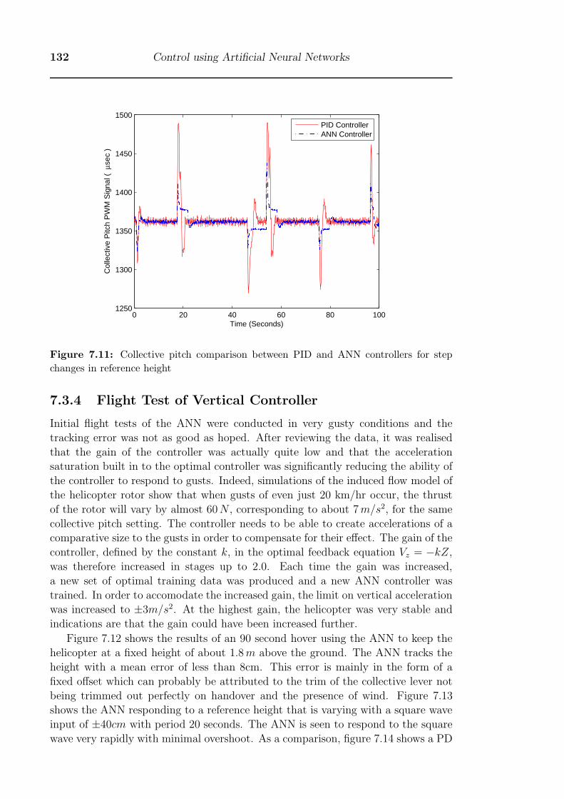
132 Control using Artificial Neural Networks
0 20 40 60 80 1001250
1300
1350
1400
1450
1500
Time (Seconds)
Col
lect
ive
Pitc
h P
WM
Sig
nal (
μsec
)
PID ControllerANN Controller
Figure 7.11: Collective pitch comparison between PID and ANN controllers for step
changes in reference height
7.3.4 Flight Test of Vertical Controller
Initial flight tests of the ANN were conducted in very gusty conditions and the
tracking error was not as good as hoped. After reviewing the data, it was realised
that the gain of the controller was actually quite low and that the acceleration
saturation built in to the optimal controller was significantly reducing the ability of
the controller to respond to gusts. Indeed, simulations of the induced flow model of
the helicopter rotor show that when gusts of even just 20 km/hr occur, the thrust
of the rotor will vary by almost 60N , corresponding to about 7m/s2, for the same
collective pitch setting. The controller needs to be able to create accelerations of a
comparative size to the gusts in order to compensate for their effect. The gain of the
controller, defined by the constant k, in the optimal feedback equation Vz = −kZ,
was therefore increased in stages up to 2.0. Each time the gain was increased,
a new set of optimal training data was produced and a new ANN controller was
trained. In order to accomodate the increased gain, the limit on vertical acceleration
was increased to ±3m/s2. At the highest gain, the helicopter was very stable and
indications are that the gain could have been increased further.
Figure 7.12 shows the results of an 90 second hover using the ANN to keep the
helicopter at a fixed height of about 1.8m above the ground. The ANN tracks the
height with a mean error of less than 8cm. This error is mainly in the form of a
fixed offset which can probably be attributed to the trim of the collective lever not
being trimmed out perfectly on handover and the presence of wind. Figure 7.13
shows the ANN responding to a reference height that is varying with a square wave
input of ±40cm with period 20 seconds. The ANN is seen to respond to the square
wave very rapidly with minimal overshoot. As a comparison, figure 7.14 shows a PD
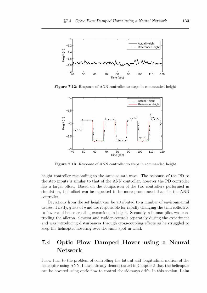
§7.4 Optic Flow Damped Hover using a Neural Network 133
40 50 60 70 80 90 100 110 120−2
−1.8
−1.6
−1.4
−1.2
−1
Time (sec)
Hei
ght (
m)
Actual HeightReference Height
Figure 7.12: Response of ANN controller to steps in commanded height
40 50 60 70 80 90 100 110 120−3
−2.5
−2
−1.5
−1
Time (sec)
Hei
ght (
m)
Actual HeightReference Height
Figure 7.13: Response of ANN controller to steps in commanded height
height controller responding to the same square wave. The response of the PD to
the step inputs is similar to that of the ANN controller, however the PD controller
has a larger offset. Based on the comparison of the two controllers performed in
simulation, this offset can be expected to be more pronounced than for the ANN
controller.
Deviations from the set height can be attributed to a number of environmental
causes. Firstly, gusts of wind are responsible for rapidly changing the trim collective
to hover and hence creating excursions in height. Secondly, a human pilot was con-
trolling the aileron, elevator and rudder controls separately during the experiment
and was introducing disturbances through cross-coupling effects as he struggled to
keep the helicopter hovering over the same spot in wind.
7.4 Optic Flow Damped Hover using a Neural
Network
I now turn to the problem of controlling the lateral and longitudinal motion of the
helicopter using ANN. I have already demonstrated in Chapter 5 that the helicopter
can be hovered using optic flow to control the sideways drift. In this section, I aim
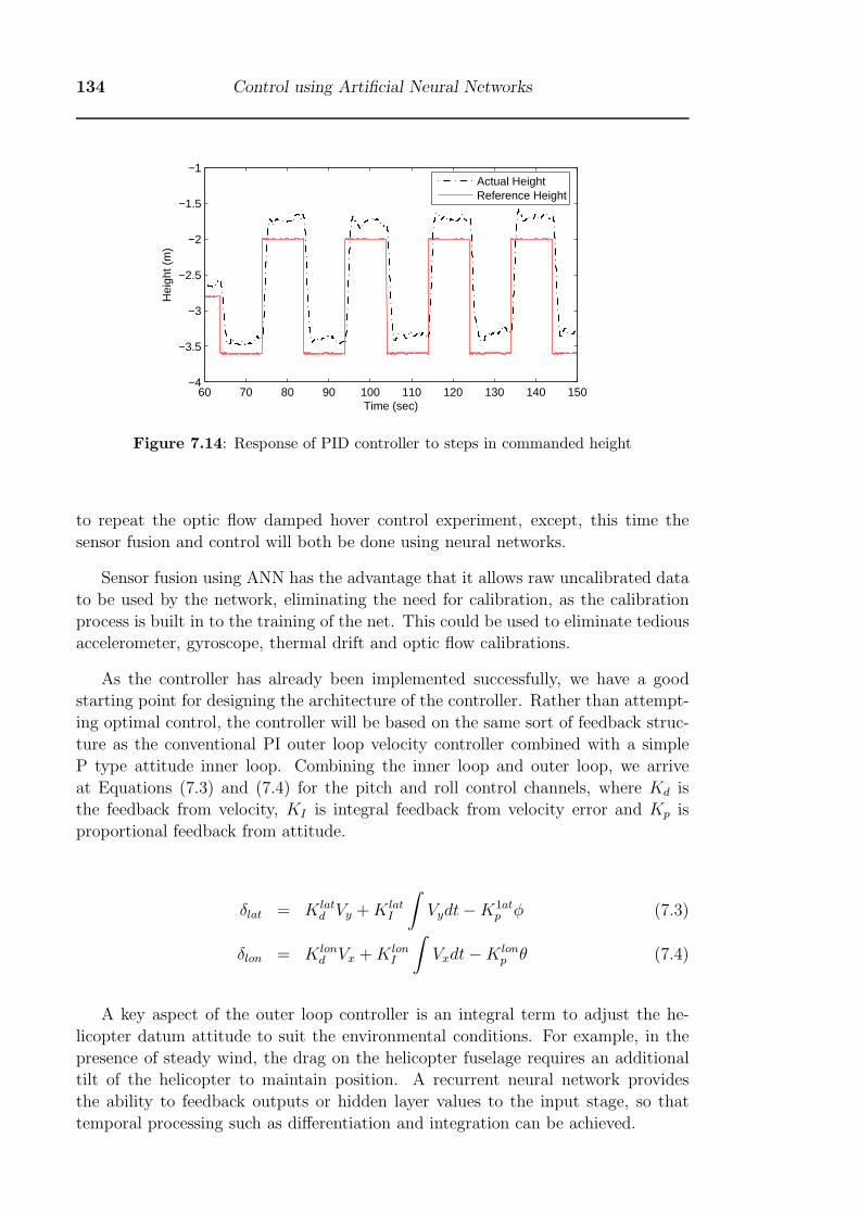
134 Control using Artificial Neural Networks
60 70 80 90 100 110 120 130 140 150−4
−3.5
−3
−2.5
−2
−1.5
−1
Time (sec)
Hei
ght (
m)
Actual HeightReference Height
Figure 7.14: Response of PID controller to steps in commanded height
to repeat the optic flow damped hover control experiment, except, this time the
sensor fusion and control will both be done using neural networks.
Sensor fusion using ANN has the advantage that it allows raw uncalibrated data
to be used by the network, eliminating the need for calibration, as the calibration
process is built in to the training of the net. This could be used to eliminate tedious
accelerometer, gyroscope, thermal drift and optic flow calibrations.
As the controller has already been implemented successfully, we have a good
starting point for designing the architecture of the controller. Rather than attempt-
ing optimal control, the controller will be based on the same sort of feedback struc-
ture as the conventional PI outer loop velocity controller combined with a simple
P type attitude inner loop. Combining the inner loop and outer loop, we arrive
at Equations (7.3) and (7.4) for the pitch and roll control channels, where Kd is
the feedback from velocity, KI is integral feedback from velocity error and Kp is
proportional feedback from attitude.
δlat = K latd Vy +K lat
I
∫Vydt−K1at
p φ (7.3)
δlon = K lond Vx +K lon
I
∫Vxdt−K lon
p θ (7.4)
A key aspect of the outer loop controller is an integral term to adjust the he-
licopter datum attitude to suit the environmental conditions. For example, in the
presence of steady wind, the drag on the helicopter fuselage requires an additional
tilt of the helicopter to maintain position. A recurrent neural network provides
the ability to feedback outputs or hidden layer values to the input stage, so that
temporal processing such as differentiation and integration can be achieved.
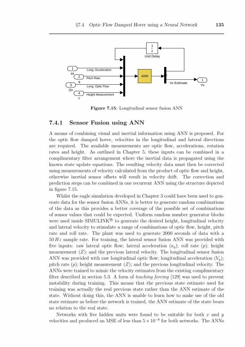
§7.4 Optic Flow Damped Hover using a Neural Network 135
Vx Estimate1
Vx
z
1
Unit Delay
ANN emu
4
z
3
Qx
2
q
1
axLong. Acceleration
Pitch Rate
Long. Optic Flow
Height Measurement
Figure 7.15: Longitudinal sensor fusion ANN
7.4.1 Sensor Fusion using ANN
A means of combining visual and inertial information using ANN is proposed. For
the optic flow damped hover, velocities in the longitudinal and lateral directions
are required. The available measurements are optic flow, accelerations, rotation
rates and height. As outlined in Chapter 5, these inputs can be combined in a
complimentary filter arrangement where the inertial data is propagated using the
known state update equations. The resulting velocity data must then be corrected
using measurements of velocity calculated from the product of optic flow and height,
otherwise inertial sensor offsets will result in velocity drift. The correction and
prediction steps can be combined in one recurrent ANN using the structure depicted
in figure 7.15.
Whilst the eagle simulation developed in Chapter 3 could have been used to gen-
erate data for the sensor fusion ANNs, it is better to generate random combinations
of the data as this provides a better coverage of the possible set of combinations
of sensor values that could be expected. Uniform random number generator blocks
were used inside SIMULINK R© to generate the desired height, longitudinal velocity
and lateral velocity to stimulate a range of combinations of optic flow, height, pitch
rate and roll rate. The plant was used to generate 2000 seconds of data with a
50Hz sample rate. For training, the lateral sensor fusion ANN was provided with
five inputs: raw lateral optic flow; lateral acceleration (ay); roll rate (p); height
measurement (Z); and the previous lateral velocity. The longitudinal sensor fusion
ANN was provided with raw longitudinal optic flow; longitudinal acceleration (Vy);
pitch rate (p); height measurement (Z); and the previous longitudinal velocity. The
ANNs were trained to mimic the velocity estimates from the existing complimentary
filter described in section 5.3. A form of teaching forcing [129] was used to prevent
instability during training. This means that the previous state estimate used for
training was actually the real previous state rather than the ANN estimate of the
state. Without doing this, the ANN is unable to learn how to make use of the old
state estimate as before the network is trained, the ANN estimate of the state bears
no relation to the real state.
Networks with five hidden units were found to be suitable for both x and y
velocities and produced an MSE of less than 5×10⁻⁸ for both networks. The ANNs
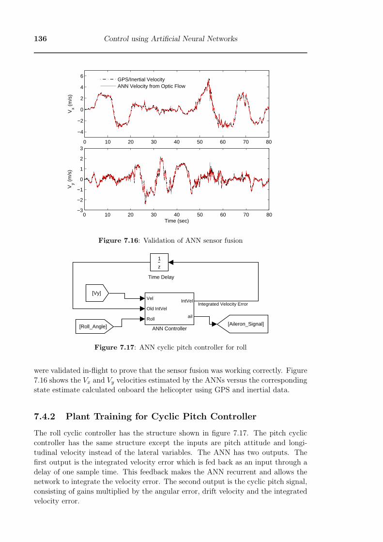
136 Control using Artificial Neural Networks
0 10 20 30 40 50 60 70 80
−4
−2
0
2
4
6V
x (m
/s)
GPS/Inertial VelocityANN Velocity from Optic Flow
0 10 20 30 40 50 60 70 80−3
−2
−1
0
1
2
3
Vy (
m/s
)
Time (sec)
Figure 7.16: Validation of ANN sensor fusion
Time Delay
z
1
[Roll_Angle]
[Vy]
[Aileron_Signal]
Vel
Old IntVel
Roll
IntVel
ail
ANN Controller
Integrated Velocity Error
Figure 7.17: ANN cyclic pitch controller for roll
were validated in-flight to prove that the sensor fusion was working correctly. Figure
7.16 shows the Vx and Vy velocities estimated by the ANNs versus the corresponding
state estimate calculated onboard the helicopter using GPS and inertial data.
7.4.2 Plant Training for Cyclic Pitch Controller
The roll cyclic controller has the structure shown in figure 7.17. The pitch cyclic
controller has the same structure except the inputs are pitch attitude and longi-
tudinal velocity instead of the lateral variables. The ANN has two outputs. The
first output is the integrated velocity error which is fed back as an input through a
delay of one sample time. This feedback makes the ANN recurrent and allows the
network to integrate the velocity error. The second output is the cyclic pitch signal,
consisting of gains multiplied by the angular error, drift velocity and the integrated
velocity error.
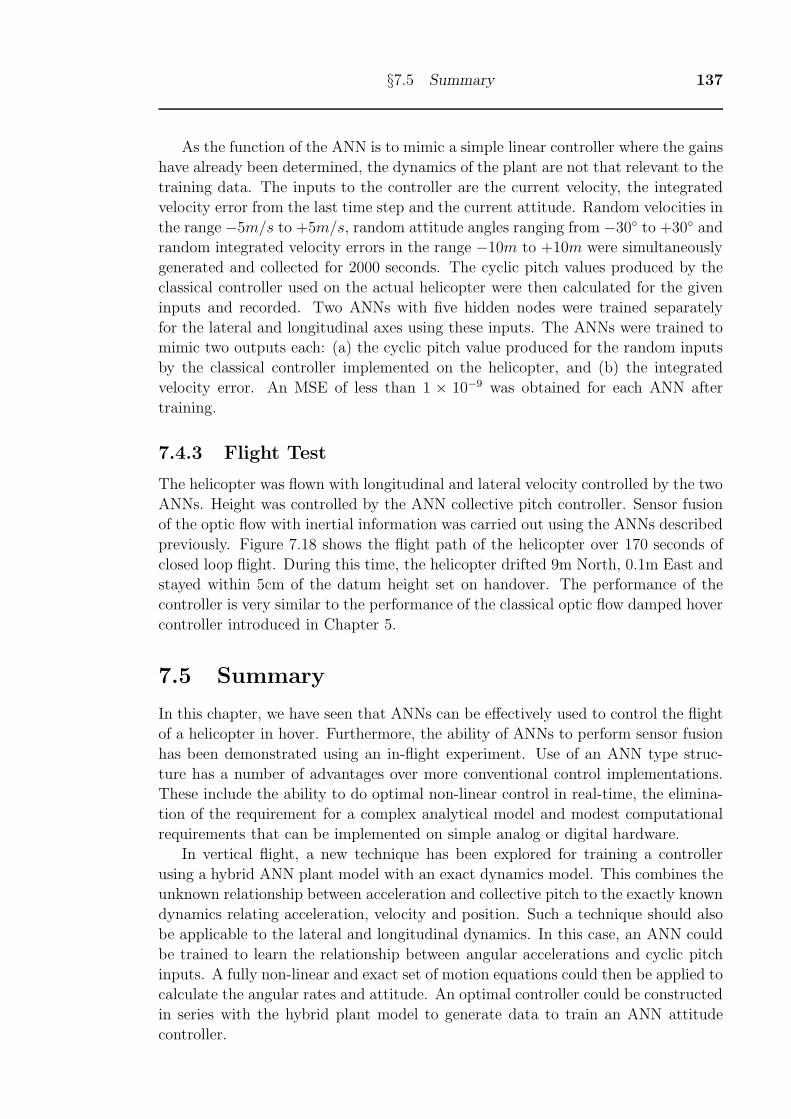
§7.5 Summary 137
As the function of the ANN is to mimic a simple linear controller where the gains
have already been determined, the dynamics of the plant are not that relevant to the
training data. The inputs to the controller are the current velocity, the integrated
velocity error from the last time step and the current attitude. Random velocities in
the range −5m/s to +5m/s, random attitude angles ranging from −30◦ to +30◦ and
random integrated velocity errors in the range −10m to +10m were simultaneously
generated and collected for 2000 seconds. The cyclic pitch values produced by the
classical controller used on the actual helicopter were then calculated for the given
inputs and recorded. Two ANNs with five hidden nodes were trained separately
for the lateral and longitudinal axes using these inputs. The ANNs were trained to
mimic two outputs each: (a) the cyclic pitch value produced for the random inputs
by the classical controller implemented on the helicopter, and (b) the integrated
velocity error. An MSE of less than 1 × 10⁻⁹ was obtained for each ANN after
training.
7.4.3 Flight Test
The helicopter was flown with longitudinal and lateral velocity controlled by the two
ANNs. Height was controlled by the ANN collective pitch controller. Sensor fusion
of the optic flow with inertial information was carried out using the ANNs described
previously. Figure 7.18 shows the flight path of the helicopter over 170 seconds of
closed loop flight. During this time, the helicopter drifted 9m North, 0.1m East and
stayed within 5cm of the datum height set on handover. The performance of the
controller is very similar to the performance of the classical optic flow damped hover
controller introduced in Chapter 5.
7.5 Summary
In this chapter, we have seen that ANNs can be effectively used to control the flight
of a helicopter in hover. Furthermore, the ability of ANNs to perform sensor fusion
has been demonstrated using an in-flight experiment. Use of an ANN type struc-
ture has a number of advantages over more conventional control implementations.
These include the ability to do optimal non-linear control in real-time, the elimina-
tion of the requirement for a complex analytical model and modest computational
requirements that can be implemented on simple analog or digital hardware.
In vertical flight, a new technique has been explored for training a controller
using a hybrid ANN plant model with an exact dynamics model. This combines the
unknown relationship between acceleration and collective pitch to the exactly known
dynamics relating acceleration, velocity and position. Such a technique should also
be applicable to the lateral and longitudinal dynamics. In this case, an ANN could
be trained to learn the relationship between angular accelerations and cyclic pitch
inputs. A fully non-linear and exact set of motion equations could then be applied to
calculate the angular rates and attitude. An optimal controller could be constructed
in series with the hybrid plant model to generate data to train an ANN attitude
controller.
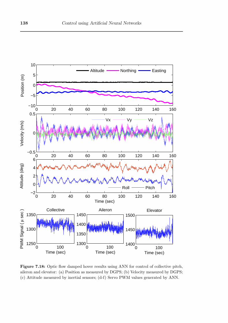
138 Control using Artificial Neural Networks
0 20 40 60 80 100 120 140 160−10
−5
0
5
10
Pos
ition
(m
)
Altitude Northing Easting
0 20 40 60 80 100 120 140 160−0.5
0
0.5
Vel
ocity
(m
/s) Vx Vy Vz
0 20 40 60 80 100 120 140 160−2
0
2
4
6
Atti
tude
(de
g)
Time (sec)
Roll Pitch
0 1001250
1300
1350
PW
M S
igna
l ( μ
sec
)
Time (sec)
Collective
0 1001300
1350
1400
1450
Time (sec)
Aileron
0 1001400
1450
1500
Time (sec)
Elevator
Figure 7.18: Optic flow damped hover results using ANN for control of collective pitch,
aileron and elevator: (a) Position as measured by DGPS; (b) Velocity measured by DGPS;
(c) Attitude measured by inertial sensors; (d-f) Servo PWM values generated by ANN.
§7.5 Summary 139
In this work I have not tested the limits of stability for the optimal controller.
In future work, the gain k in the feedback equation Vz = −kz could be increased
in steps to determine at what point the control loop becomes unstable or the effect
of noise becomes too great. Increasing the gain will improve tracking performance.
Steady state offsets in height due to collective pitch trim errors might be reduced
further by introducing integral feedback in parallel with the ANN controller. The
effect of the integral control on the stability of the ANN should be investigated in
future work.

Chapter 8
Advanced Sensor Fusion
8.1 Introduction
The simple fusion techniques used so far in this thesis have been adequate for demon-
strating closed loop control of the helicopters, but have had some shortcomings re-
lated to ignoring sensor errors. The main problem experienced is that the inertial
sensors suffer drift, which arises because the sensor offsets change with temperature.
In this chapter, I attempt to address these problems by exploring online sensor error
estimation using Extended Kalman Filters (EKF).
8.1.1 Overview of the Discrete EKF Algorithm
A Kalman filter is a recursive filter that can provide an optimal estimate of the
states of a linear dynamical system given noisy measurements of the system. The
development of the Kalman filter is largely attributed to Rudolf Kalman [209] who
the filter is named after. An Extended Kalman Filter (EKF), first proposed by
Schmidt [210], is an extension of the Kalman filter where the state update equations
and relationship between the measurements and the states is not linear. The EKF
is an ad-hoc technique [211] which is not optimal owing to the linearisation that is
used to propagate the filter. Both Kalman filters and EKF can be used to estimate
states that are not directly measured. For example, in the case of vertical flight, an
EKF could be used to estimate vertical velocity given only acceleration and height,
but no direct measure of w. The downside of using an EKF is that it requires a
higher level of computational overhead than a simple filter and in some cases may
diverge or fail numerically.
A discrete EKF assumes a non-linear dynamic model defined by:
xk = f (xk−1, k − 1) + wk (8.1)
where xk is the kth estimate of the state variables and wk is process noise. The
non-linear measurement model for the EKF is defined by:
zk = h (xk, k) + vk (8.2)
The measurement and plant noise vk and wk are assumed to be zero-mean
Gaussian sequences. The EKF algorithm is implemented by solving the following
set of equations recursively:
141
142 Advanced Sensor Fusion
Computing the predicted state estimate:
x−k = f
(x+k−1, k − 1
)(8.3)
Computing the predicted measurement:
zk = h(x−k , k) (8.4)
Linear approximation equation:
Φk−1 ≈ ∂f (x, k − 1)
∂x
∣∣∣∣x=x
−
k
(8.5)
Conditioning the predicted estimate on the measurement:
x+k = x−
k + Kk(zk − zk) (8.6)
Hk ≈ ∂h(x, k)
∂x
∣∣∣∣z=x
−
k
(8.7)
Computing the a priori covariance matrix:
P−k = Φk−1P k−1Φ
Tk−1 + Qk−1 (8.8)
Computing the Kalman gain:
Kk = P−k HT
k [HkP−k HT
k + Rk]−1 (8.9)
Computing the a posteriori covariance matrix:
P +k = (I − KkHk) P−
k (8.10)
The Q and R matrices represent the process and measurement noise respectively.
They are approximately represented by diagonal matrices having the diagonal terms
set equal to the statistical variance of the noise.
In the EKFs described in this chapter, only first order approximations to the
fundamental matrix Φ will be used, since use of higher order approximations do not
generally lead to an improvement in the performance of the EKF [212].
8.2 Attitude Estimation
The gyroscopes used on the Eagle helicopter are subject to thermal drift, which
requires either: (a) constant zeroing in the field to eliminate the offsets, or (b)
switching the avionics on and then waiting for up to an hour for the gyroscope
temperatures to stabilise before use. A system that could estimate the gyroscope
offset errors in real-time to provide a corrected gyroscope rate output would therefore
§8.2 Attitude Estimation 143
be very useful. Two methods of achieving this using EKF were devised and simulated
for comparison. The aim of each EKF algorithm was to determine the gyroscope
offsets dynamically, but not to estimate the gyroscope scale and misalignment errors
as they could be removed by calibration as described in Appendix C and were not
able to change appreciably post-calibration. Each EKF algorithm was tested using
simulated sensor data for the helicopter in hover. The algorithm and results are
described separately below.
8.2.1 EKF Algorithm One
This algorithm propogates a nine element state vector consisting of a unit vector
(g) representing the direction of gravity, a unit vector (b) representing the earth’s
magnetic field and the three gyroscope offsets. The unit vectors define the direc-
tions relative to the helicopter body axes. The observations for this algorithm are
the measured acceleration and magnetic vectors. Because both the observations of
attitude and the representation of attitude are in vector form, the correction of the
state estimate is already linear, and does not need to be linearised. This means that
observations with large deviations from mean do not violate linearity assumptions
and therefore very noisy observations can be tolerated. Also, because the magnetic
and accelerometer vectors are independently stored, the algorithm can continue in
a degraded mode when one sensor fails. The state vector for this algorithm is:
x =[gx gy gz bx by bz δx δy δz
]T(8.11)
where g = [gx gy gz]T , b = [bx by bz]
T and δ = [δx δy δz]T are the gravity direction
unit vector, magnetic direction unit vector and gyroscope offset vectors respectively.
The vectors are subject to body axis rotation rates defined by the symbols P,Q and
R which are equal to the sum of the measured gyroscope rates (p, q and r) and the
gyroscope offsets δx, δy and δz as in Equation (8.12).
P = p + δp, Q = q + δq, R = r + δr (8.12)
The change in the vectors due to P,Q and R over a time step ΔT can be expressed
as a rotation matrix. To determine this rotation matrix, first consider Equation
(8.13) which describes the effect of these rotation rates on the attitude quaternion:⎡⎢⎢⎣q0q1q2q3
⎤⎥⎥⎦ = −1
2
⎡⎢⎢⎣0 P Q R
−P 0 −R Q
−Q R 0 −P−R −Q P 0
⎤⎥⎥⎦T ⎡⎢⎢⎣
q0q1q2q3
⎤⎥⎥⎦ (8.13)
or in more compact form
dq
dt= −1
2Ωq (8.14)
where q is the vector of quaternion paramaters [q0 q1 q2 q3]T and Ω is the angular
velocity tensor. For sufficiently small ΔT , this can be approximated with the first
144 Advanced Sensor Fusion
order expression in Equation (8.15).
Δq ≈ −1
2ΩqΔT (8.15)
As we are only interested in the change of the vectors relative to the existing
body axes then we can set the quaternion on the right hand side of Equation (8.15)
to q = [1 0 0 0]T corresponding to a datum attitude. The change in attitude over the
time step is then given by Equation (8.16).⎡⎢⎢⎣Δq0Δq1Δq2Δq3
⎤⎥⎥⎦ =1
2
⎡⎢⎢⎣0
P
Q
R
⎤⎥⎥⎦ΔT (8.16)
Hence the change in attitude over the time-step relative to the body axes is:⎡⎢⎢⎣q0q1q2q3
⎤⎥⎥⎦ =
⎡⎢⎢⎣1
PΔT/2
QΔT/2
RΔT/2
⎤⎥⎥⎦ =
⎡⎢⎢⎣1
P
Q
R
⎤⎥⎥⎦ (8.17)
where the definitions below have been used to simplify the expression:
P = PΔT
2, Q = Q
ΔT
2, R = R
ΔT
2(8.18)
The effect of this change in attitude on the g and b vectors can be determined
by a 3 × 3 rotation matrix B. The complete state transition matrix is given below
where Bij are the elements of B.
⎡⎢⎢⎢⎢⎢⎢⎢⎢⎢⎢⎢⎢⎢⎣
gxgygzbxbybzδpδqδr
⎤⎥⎥⎥⎥⎥⎥⎥⎥⎥⎥⎥⎥⎥⎦k+1
= F (x, k) =
⎡⎢⎢⎢⎢⎢⎢⎢⎢⎢⎢⎢⎢⎢⎣
B11 B12 B13 0 0 0 0 0 0
B21 B22 B23 0 0 0 0 0 0
B31 B32 B33 0 0 0 0 0 0
0 0 0 B11 B12 B13 0 0 0
0 0 0 B21 B22 B23 0 0 0
0 0 0 B31 B32 B13 0 0 0
0 0 0 0 0 0 1 0 0
0 0 0 0 0 0 0 1 0
0 0 0 0 0 0 0 0 1
⎤⎥⎥⎥⎥⎥⎥⎥⎥⎥⎥⎥⎥⎥⎦
⎡⎢⎢⎢⎢⎢⎢⎢⎢⎢⎢⎢⎢⎢⎣
gxgygzbxbybzδpδqδr
⎤⎥⎥⎥⎥⎥⎥⎥⎥⎥⎥⎥⎥⎥⎦k
(8.19)
The rotation matrix B is defined in terms of quaternion parameters as:
B =
⎡⎣ q20 + q2
1 − q22 − q2
3 2 (q1q2 + q0q3) 2 (q1q2 + q0q3)
2 (q1q2 − q0q3) q20 + q2
1 − q22 − q2
3 2 (q2q3 + q0q1)
2 (q1q3 + q1q2) 2 (q2q3 − q0q1) q20 − q2
1 − q22 + q2
3
⎤⎦ (8.20)
Using the quaternion attitude change in Equation (8.17), this becomes:
§8.2 Attitude Estimation 145
B =
⎡⎣ 1 0 0
0 1 0
0 0 1
⎤⎦+
⎡⎣ P 2 − Q2 − R2 2(P Q+ R
)2(P R + Q
)2(P Q+ R
) −P 2 + Q2 − R2 2(QR+ P
)2(P R + Q
)2(QR− P
) −P 2 − Q2 + R2
⎤⎦ (8.21)
For the sake of brevity, only the state-update for the x-gravity component will be
shown. In scalar form, the state update for gx can be found from Equation (8.19):
gk+1x = gkx +
ΔT 2
4
((p+ δp)2 − (q + δq)2 − (r + δr)2 −) gkx
+
(ΔT 2
2(p+ δp) (q + δq) + ΔT (r + δr)
)gky
+
(ΔT 2
2(p+ δp) (r + δr) − ΔT (q + δq)
)gkz (8.22)
In order to derive the fundamental matrix, Φ, this equation is differentiated
with respect to each state variable resulting in Equations (8.23-8.28). Each partial
derivative of gx forms a unique column of the first row of Φ.
∂gk+1x
∂gkx= 1 +
ΔT 2
4
((p+ δp)2 − (q + δq)2 − (r + δr)2) (8.23)
∂gk+1x
∂gky=
ΔT 2
2
(ΔT 2
2(p+ δp) (q + δq) + ΔT (r + δr)
)(8.24)
∂gk+1x
∂gkz=
ΔT 2
2
(ΔT 2
2(p+ δp) (r + δr) − ΔT (q + δq)
)(8.25)
∂gk+1x
∂δkp=
ΔT 2
2(p+ δp) gkx +
ΔT 2
2(q + δq) gky +
ΔT 2
2(r + δr) gkz (8.26)
∂gk+1x
∂δkq= −ΔT 2
2(q + δq) gkx +
ΔT 2
2(p+ δp) gky − ΔTgkz (8.27)
∂gk+1x
∂δkr= −ΔT 2
2(r + δr) gkx + ΔTgky +
ΔT 2
2(p+ δp) gkz (8.28)
Similarly, the scalar equation of gy is differentiated with respect to each state
variable to form the second row of Φ. A row is created for each state variable to
create the entire Φ matrix.
The observations are the six normalised vector components so that the measure-
ment matrix is linear and time invariant. Hence:
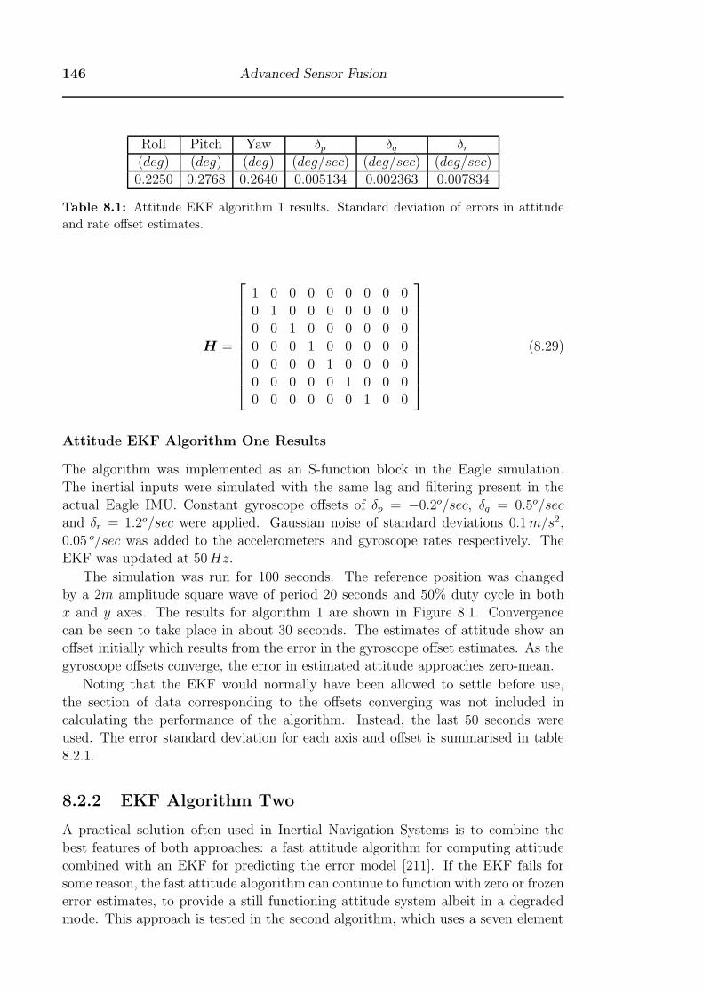
146 Advanced Sensor Fusion
Roll Pitch Yaw δp δq δr(deg) (deg) (deg) (deg/sec) (deg/sec) (deg/sec)0.2250 0.2768 0.2640 0.005134 0.002363 0.007834
Table 8.1: Attitude EKF algorithm 1 results. Standard deviation of errors in attitude
and rate offset estimates.
H =
⎡⎢⎢⎢⎢⎢⎢⎢⎢⎢⎣
1 0 0 0 0 0 0 0 0
0 1 0 0 0 0 0 0 0
0 0 1 0 0 0 0 0 0
0 0 0 1 0 0 0 0 0
0 0 0 0 1 0 0 0 0
0 0 0 0 0 1 0 0 0
0 0 0 0 0 0 1 0 0
⎤⎥⎥⎥⎥⎥⎥⎥⎥⎥⎦(8.29)
Attitude EKF Algorithm One Results
The algorithm was implemented as an S-function block in the Eagle simulation.
The inertial inputs were simulated with the same lag and filtering present in the
actual Eagle IMU. Constant gyroscope offsets of δp = −0.2o/sec, δq = 0.5o/sec
and δr = 1.2o/sec were applied. Gaussian noise of standard deviations 0.1m/s2,
0.05 o/sec was added to the accelerometers and gyroscope rates respectively. The
EKF was updated at 50Hz.
The simulation was run for 100 seconds. The reference position was changed
by a 2m amplitude square wave of period 20 seconds and 50% duty cycle in both
x and y axes. The results for algorithm 1 are shown in Figure 8.1. Convergence
can be seen to take place in about 30 seconds. The estimates of attitude show an
offset initially which results from the error in the gyroscope offset estimates. As the
gyroscope offsets converge, the error in estimated attitude approaches zero-mean.
Noting that the EKF would normally have been allowed to settle before use,
the section of data corresponding to the offsets converging was not included in
calculating the performance of the algorithm. Instead, the last 50 seconds were
used. The error standard deviation for each axis and offset is summarised in table
8.2.1.
8.2.2 EKF Algorithm Two
A practical solution often used in Inertial Navigation Systems is to combine the
best features of both approaches: a fast attitude algorithm for computing attitude
combined with an EKF for predicting the error model [211]. If the EKF fails for
some reason, the fast attitude alogorithm can continue to function with zero or frozen
error estimates, to provide a still functioning attitude system albeit in a degraded
mode. This approach is tested in the second algorithm, which uses a seven element
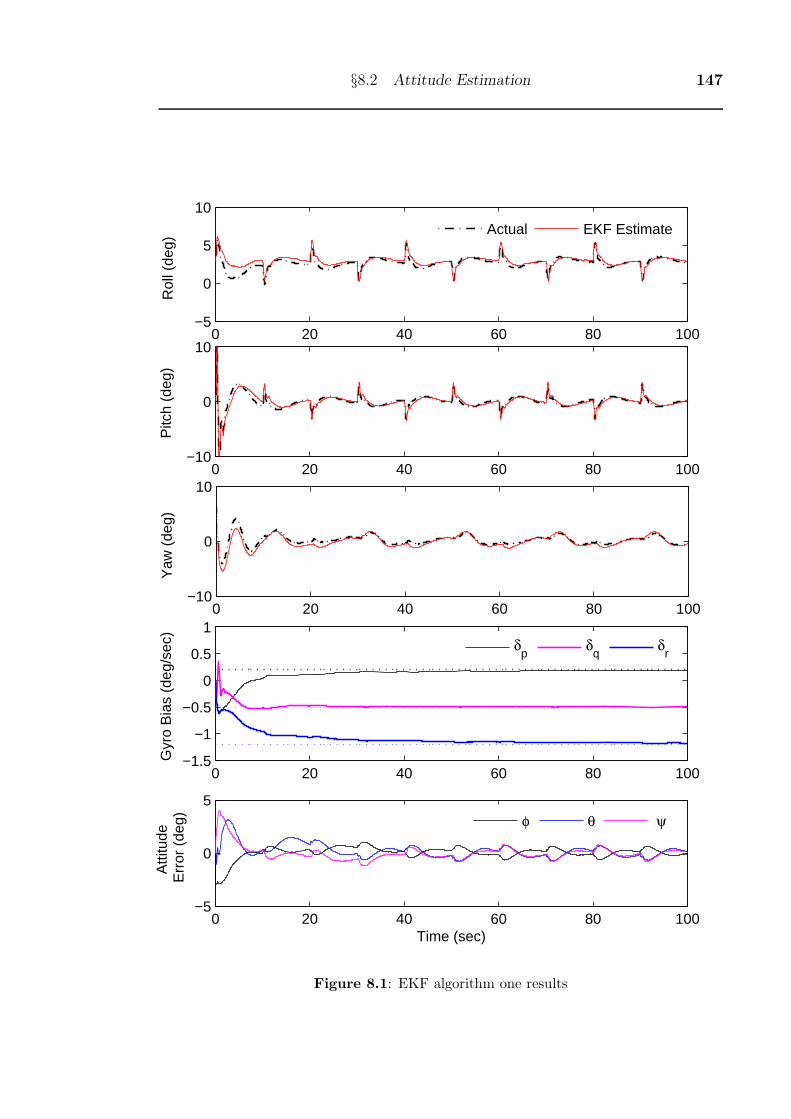
§8.2 Attitude Estimation 147
0 20 40 60 80 100−5
0
5
10
Rol
l (de
g)
Actual EKF Estimate
0 20 40 60 80 100−10
0
10
Pitc
h (d
eg)
0 20 40 60 80 100−10
0
10
Yaw
(de
g)
0 20 40 60 80 100−1.5
−1
−0.5
0
0.5
1
Gyr
o B
ias
(deg
/sec
)
δp
δq
δr
0 20 40 60 80 100−5
0
5
Atti
tude
Err
or (
deg)
Time (sec)
φ θ ψ
Figure 8.1: EKF algorithm one results
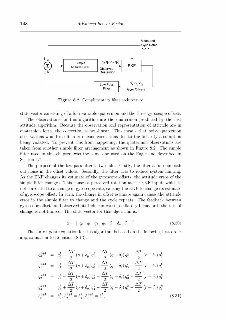
148 Advanced Sensor Fusion
[q0 q1 q2 q3]
Low Pass
Filter
Σ
Measured
Gyro Rates
p,q,r
Observed Quaternion
Gyro Offsets
δx δy δz
+
-
Simple
Attitude Filter EKFΣ
Figure 8.2: Complimentary filter architecture
state vector consisting of a four-variable quaternion and the three gyroscope offsets.
The observations for this algorithm are the quaternion produced by the fast
attitude algorithm. Because the observation and representation of attitude are in
quaternion form, the correction is non-linear. This means that noisy quaternion
observations would result in erroneous corrections due to the linearity assumption
being violated. To prevent this from happening, the quaternion observations are
taken from another simple filter arrangement as shown in Figure 8.2. The simple
filter used in this chapter, was the same one used on the Eagle and described in
Section 4.7.
The purpose of the low-pass filter is two fold. Firstly, the filter acts to smooth
out noise in the offset values. Secondly, the filter acts to reduce system hunting.
As the EKF changes its estimate of the gyroscope offsets, the attitude error of the
simple filter changes. This causes a perceived rotation at the EKF input, which is
not correlated to a change in gyroscope rate, causing the EKF to change its estimate
of gyroscope offset. In turn, the change in offset estimate again causes the attitude
error in the simple filter to change and the cycle repeats. The feedback between
gyroscope offsets and observed attitude can cause oscillatory behavior if the rate of
change is not limited. The state vector for this algorithm is:
x =[q0 q1 q2 q3 δp δq δr
]T(8.30)
The state update equation for this algorithm is based on the following first order
approximation to Equation (8.13):
qk+10 = qk0 − ΔT
2(p+ δp) q
k1 − ΔT
2(q + δq) q
k2 −
ΔT
2(r + δr) q
k3
qk+11 = qk1 − ΔT
2(p+ δp) q
k0 +
ΔT
2(q + δq) q
k3 − ΔT
2(r + δr) q
k2
qk+12 = qk2 − ΔT
2(p+ δp) q
k3 − ΔT
2(q + δq) q
k0 −
ΔT
2(r + δr) q
k1
qk+13 = qk3 +
ΔT
2(p+ δp) q
k4 −
ΔT
2(q + δq) q
k4 − ΔT
2(r + δr) q
k4
δk+1p = δkp , δ
k+1q = δkq , δ
k+1r = δkr , (8.31)

§8.3 Attitude EKF Discussion 149
δp δq δrRaw 0.01657o/sec 0.02123o/sec 0.01755o/sec
Filtered 0.007746o/sec 0.006431o/sec 0.006557o/sec
Table 8.2: EKF algorithm 2 - standard deviation of errors in raw and filtered rate offset
estimates.
Roll Pitch Yaw0.3221o 0.4053o 0.3745o
Table 8.3: EKF algorithm 2 - standard deviation of errors in attitude.
Using the same process used for algorithm one the Φ matrix can be derived. The
measurement matrix H is:
H =
⎡⎢⎢⎣1 0 0 0 0 0 0 0 0
0 1 0 0 0 0 0 0 0
0 0 1 0 0 0 0 0 0
0 0 0 1 0 0 0 0 0
⎤⎥⎥⎦ (8.32)
Attitude EKF Algorithm Two Results
The second algorithm was tested using the same sensor errors and helicopter mo-
tions as for algorithm one. The results for algorithm two are shown in Figure 8.3.
Convergence can be seen to have taken place in about 50 seconds, but the raw
prediction of offsets is very noisy and not useable without filtering. As the rate of
change of the gyroscope offsets is known to be very slow, heavy low pass filtering is
possible. The black lines in Figure 8.3 show the filtered values of gyroscope offset
after passing through a 2-pole Butterworth filter with a time constant of 50 seconds.
8.3 Attitude EKF Discussion
Both EKFs tested showed an initial spike in the offset estimations of up to 5o/sec.
This spike occurs as the EKF is poorly converged after initialisation. This spike
would not be so marked in normal operation because the gyroscope offsets would be
zeroed prior to starting the EKF algorithm.
In both algorithms, the assumption is made that the average observation of the
gravity vector is pointing straight down. This assumption is not true in the general
case, as the vehicle is subject to g-force when maneovering and the accelerometers
actually measure the sum of the earth’s gravity and the vehicle acceleration. Hence,
if the helicopter was placed in a sustained banked turn, the gravity vector measured
by the accelerometers would, in fact, be tilted away from the direction of turn. Using
either algorithm would result in a level attitude estimate despite the angle of bank.

150 Advanced Sensor Fusion
0 20 40 60 80 100−5
0
5
10
Rol
l (de
g)
Actual EKF Estimate
0 20 40 60 80 100−10
0
10
Pitc
h (d
eg)
0 20 40 60 80 100−10
0
10
Yaw
(de
g)
0 20 40 60 80 100−1
0
1
δ p (de
g/s)
Smoothed Bias Raw Bias Actual Bias
0 20 40 60 80 100−2
0
2
δ q (de
g/s)
0 20 40 60 80 100−5
0
5
δ r (de
g/s)
0 20 40 60 80 100−5
0
5
Atti
tude
Err
or (
deg)
Time (sec)
φ θ ψ
Figure 8.3: EKF algorithm two results

§8.4 Velocity and Height Estimation 151
The same errors will arise whenever the helicopter accelerates along one of its axes.
For example, if the helicopter was to accelerate forwards and stay level, the pitch
attitude estimate would indicate a nose-up attitude that did not exist. One solution
to this problem would be to make use of GPS to determine the absolute accelerations,
so that the GPS acceleration could be subtracted from the accelerometer reading
before it was used as an observation [213–215].
The best performing filter in terms of estimate accuracy is algorithm one. This
nine state algorithm uses a linear correction step, which gives it the greatest advan-
tage in terms of robustness. This algorithm is the recommended choice for embedded
application in the autopilot.
8.4 Velocity and Height Estimation
Optic flow provides the helicopter with observations of longitudinal and lateral ve-
locity, u and v. A measurement of height above terrain (Z) may be obtained from
a laser rangefinder, a downwards looking stereo camera, or by comparing GPS al-
titude with a known terrain height. Additional inertial data from accelerometers
and gyroscopes can be used to update the velocity estimates. In order for stable
control of height to be achieved, one unmeasured state, vertical velocity w, is re-
quired. The obvious choice of algorithm for fusing these sensor data and predicting
the unmeasured state is the Extended Kalman Filter.
The accelerometer offset in the Eagle IMU can be mostly eliminated using accu-
rate thermal calibration as each accelerometer is fitted with an on-chip temperature
sensor. However, this may not be the case with all other IMU implementations. In
addition, offset errors may still arise from errors in attitude due to IMU misalignment
during installation. The effect of neglecting these errors is a biased velocity estimate.
In the case of the optic flow damped hover controller, such a bias would cause the
helicopter to continually drift in one direction. The solution to this problem may
be to use an EKF to predict the biases in x, y and z acceleration measurements.
The seven state representation chosen for the EKF, provided at Equation (8.33),
includes the velocity estimates, acceleration offsets and height.
x =[u v w δx δy δz Z ] (8.33)
For a small enough time step, the state update equations can be written directly
from the rigid body equations of motion using a first order approximation as:
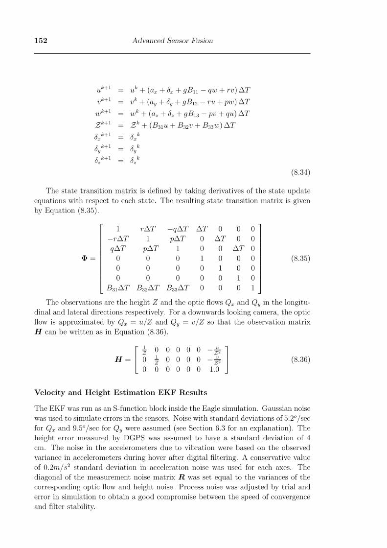
152 Advanced Sensor Fusion
uk+1 = uk + (ax + δx + gB11 − qw + rv)ΔT
vk+1 = vk + (ay + δy + gB12 − ru+ pw)ΔT
wk+1 = wk + (az + δz + gB13 − pv + qu)ΔT
Zk+1 = Zk + (B31u+B32v +B33w)ΔT
δxk+1 = δx
k
δyk+1 = δy
k
δzk+1 = δz
k
(8.34)
The state transition matrix is defined by taking derivatives of the state update
equations with respect to each state. The resulting state transition matrix is given
by Equation (8.35).
Φ =
⎡⎢⎢⎢⎢⎢⎢⎢⎢⎢⎣
1 rΔT −qΔT ΔT 0 0 0
−rΔT 1 pΔT 0 ΔT 0 0
qΔT −pΔT 1 0 0 ΔT 0
0 0 0 1 0 0 0
0 0 0 0 1 0 0
0 0 0 0 0 1 0
B31ΔT B32ΔT B33ΔT 0 0 0 1
⎤⎥⎥⎥⎥⎥⎥⎥⎥⎥⎦(8.35)
The observations are the height Z and the optic flows Qx and Qy in the longitu-
dinal and lateral directions respectively. For a downwards looking camera, the optic
flow is approximated by Qx = u/Z and Qy = v/Z so that the observation matrix
H can be written as in Equation (8.36).
H =
⎡⎣ 1Z 0 0 0 0 0 − u
Z2
0 1Z
0 0 0 0 − vZ2
0 0 0 0 0 0 1.0
⎤⎦ (8.36)
Velocity and Height Estimation EKF Results
The EKF was run as an S-function block inside the Eagle simulation. Gaussian noise
was used to simulate errors in the sensors. Noise with standard deviations of 5.2o/sec
for Qx and 9.5o/sec for Qy were assumed (see Section 6.3 for an explanation). The
height error measured by DGPS was assumed to have a standard deviation of 4
cm. The noise in the accelerometers due to vibration were based on the observed
variance in accelerometers during hover after digital filtering. A conservative value
of 0.2m/s2 standard deviation in acceleration noise was used for each axes. The
diagonal of the measurement noise matrix R was set equal to the variances of the
corresponding optic flow and height noise. Process noise was adjusted by trial and
error in simulation to obtain a good compromise between the speed of convergence
and filter stability.
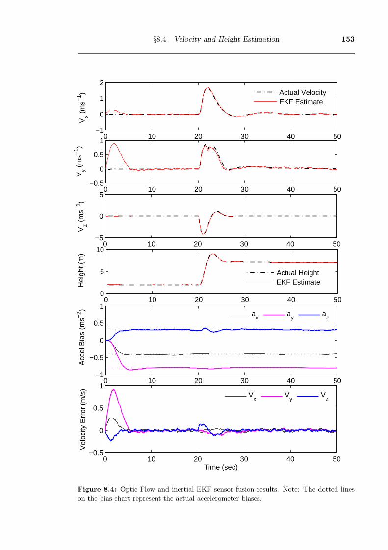
§8.4 Velocity and Height Estimation 153
0 10 20 30 40 50−1
0
1
2V
x (m
s−1 ) Actual Velocity
EKF Estimate
0 10 20 30 40 50−0.5
0
0.5
1
Vy (
ms−
1 )
0 10 20 30 40 50−5
0
5
Vz (
ms−
1 )
0 10 20 30 40 500
5
10
Hei
ght (
m)
Actual HeightEKF Estimate
0 10 20 30 40 50−1
−0.5
0
0.5
1
Acc
el B
ias
(ms−
2 )
ax
ay
az
0 10 20 30 40 50−0.5
0
0.5
1
Vel
ocity
Err
or (
m/s
)
Time (sec)
Vx
Vy
Vz
Figure 8.4: Optic Flow and inertial EKF sensor fusion results. Note: The dotted lines
on the bias chart represent the actual accelerometer biases.
154 Advanced Sensor Fusion
Vx Vy Vz Z δx δy δz(m/s) (m/s) (m/s) (m) (m/s2) (m/s2) (m/s2)0.0023 0.0032 0.0037 0.0160 0.012 0.012 0.018
Table 8.4: Standard deviations of attitude error and accelerometer bias estimates
The simulated accelerometer biases were set to δx = 0.3m/s2,δy = −0.4m/s2
and δz = −0.8m/s2. The simulated helicopter was subjected to a step in desired
position of 5m in x and y position, and 2m in height at 20 seconds after the simulation
was started. The results for 50 seconds are shown in Figure 8.4. Convergence of the
biases takes place in less than 10 seconds.
Table 8.4 shows the standard deviations of the attitude errors and accelerometer
bias estimates, calculated from the period of flight after the first 10 seconds when
convergence is occuring. The errors in velocity and height, after convergence, are
negligible and would be suitable for use in precision control of the helicopter in
hover. The accelerometer biases are found to within 0.02m/s2 of their true values.
8.5 Summary
In this chapter, a number of means for estimating sensor offsets have been described.
These techniques are not biologically inspired but could be used to augment an oth-
erwise biologically inspired sensing and control system. Unfortunately, due to time
constraints, flight testing of these EKF algorithms was not achieved but indications
are that they would have worked on a real platform.
In future work, it may be possible to estimate the sensor error offsets using
artificial neural networks instead of EKF, which would reduce computation time
and may help to ensure stability. Future work on sensor fusion should include
combining the attitude and velocity estimates into a single EKF. This would allow
the errors determined from one sensing mode to be used to improve the estimates
of the other. For example, the accelerometer biases found from optic flow could be
used to reduce offset errors in the attitude.
Chapter 9
Conclusions and
Recommendations
9.1 Summary of Achievements
In this thesis, techniques have been demonstrated for sensing and control for an au-
tonomous helicopter in hover and forward flight using techniques inspired by biology.
Optic flow combined with some measure of attitude from basic MEMS inertials was
shown to be sufficient to contain the drift of a helicopter in hover, and to control
the height of a helicopter in forward flight.
The use of the I2A algorithm for computing optic flow is robust in an outdoor
environment and has been shown to work sufficiently well for precision flight control
over unprepared surfaces such as tarmac, concrete and grass. The I2A algorithm
appears to be more robust than classical machine vision techniques that involve
feature tracking, owing to its ability to match over complete image patches rather
than relying on identifying and correlating specific features.
I have presented a new technique for control using neural networks. Flight tests
have confirmed that a neural network control system can achieve similar results to
an optimal trajectory controller with orders of magnitude greater computational
requirement. This makes a platform with complex open loop dynamics controllable
using simple computational hardware. I have also shown that sensor fusion of visual
and inertial information can be achieved using simple neural networks.
9.2 Areas for Future Study
9.2.1 Control of Flight using Optic Flow
Throughout the thesis other sensing modes have been combined with optic flow to
determine either range given speed or speed given range. The problem of how vision
might be used in a standalone mode without a secondary sensing mode has not been
tackled. For example, is it possible to use optic flow to determine height above ter-
rain when there is no available measure of ground speed? Preliminary experimental
work by Baird and Boeddeker [216] at the Australian National University suggest
that bees deliberately impart a lateral sinusoidal displacement of known amplitude
upon their flight path in order to generate optic flow in a defined way (a notion
155
156 Conclusions and Recommendations
suggested on theoretical grounds in 1993 by Srinivasan et al [217]). As the veloc-
ities corresponding to the lateral wiggle are a function of the amplitude, the bees
would be able to deduce range from the lateral optic flow signal and thereby control
their height. Apparently, bees can also regulate their flight speed based on the lon-
gitudinal optic flow signal [218], which explains why bees can maintain a constant
flight speed regardless of headwinds and tailwinds which may reach 50% of the bee’s
forward flight speed [219]. With range known from lateral optic flow and forward
speed known from longitudinal optic flow, the bees are able to regulate both speed
and height using the one sensory system.
One could imagine such an optic flow sensing scheme being implemented on a
helicopter. An open loop oscillation in attitude could be applied about the trim
roll reference attitude. Optic flow ranging from the assumed open loop lateral
velocity would be used to control height. Sideways drift due to wind could be
estimated and corrected based on the mean lateral optic flow over a complete lateral
oscillation. This scheme could be used equally to control hover and forward flight
of the helicopter. In the case of hover, the controller would simply act to maintain
zero longitudinal optic flow. In forward flight, the controller would aim to achieve
constant longitudinal optic flow, corresponding to the desired ground speed.
9.2.2 Computation of Optic Flow
In this thesis, optic flow was calculated with PC hardware implemented either on the
ground using telemetry or using onboard PC104 flight computers. The control by
telemetry approaches suffer problems in that telemetry degrades the quality of the
imagery and may fail completely when line of sight is lost. Considerable research
is underway towards developing autonomy for Micro Air Vehicles (MAV), which
are defined by DARPA as flight vehicles with a maximum dimension of less than
15cm [220]. PC104 hardware is comparatively heavy and much too heavy and power
consuming for implementation on an MAV. A number of researchers have proposed
using custom made integrated circuits as autopilot devices with optic flow sensing
built in [221–224]. Ultimately, this approach would lead to a lightweight system,
but the expense and long turn-around time is prohibitive in the short term.
Recent unpublished research at UNSW@ADFA has shown that use of the I2A
on an FPGA can result in data at up to 50 frames per second, which is fast enough
for flight control. FPGAs are integrated circuits containing millions of logic gates,
which can be reconfigured through software to form any desired digital processing
network. Due to their internal architecture, FPGA chips can process data in a
massively parallel way rather than the sequential fashion normally present in com-
puters, enabling real-time processing of high-bandwidth visual information. Some
other groups [225,226] have attempted optic flow on FPGA, but so far this has been
done using slower algorithms than I2A and heavier electronics implementations, not
suited for real-time control of a MAV. Research into development of an FPGA based
optic flow system using I2A may result in a combined vision sensor and autopilot
on a single chip which be suited to installation on an MAV payload.
§9.2 Areas for Future Study 157
9.2.3 Control of Position using Vision
One of the major problems of using optic flow for stabilisation in hover is that a
near perfect hover will result in a very weak optic flow signal because motions are
small. Further, optic flow does not provide for identification of landmark features
that can be used to maintain station. There is some evidence that bees make use of
a stored 2D snapshot to locate themselves [227, 228]. Cartwright and Collett [227]
suggest that the direction in which the bees move at any moment is governed by the
discrepancy between the snapshot and its current retinal image. A new algorithm is
therefore proposed that uses a stored image of the ground, a snapshot, so to speak,
taken of the ground directly under the helicopter. This snapshot would form a visual
anchor point for the helicopter. By comparing subsequent frames with this snapshot
using the I2A algorithm, it should be possible to calculate absolute translation from
the datum.
For a practical implementation, sufficient overlap between the snapshot and the
current image is neccessary. This means that the helicopter could not stray more
than about 20 percent of the helicopter height away from where the snapshot was
taken. Whenever the original image moves outside the image catchment area, a new
snapshot would have to be taken. New snapshots might also be taken from time
to time to compensate for long term environmental changes. To compensate for
perspective distortion of the image as the craft moves, it may be necessary to trans-
form the snapshot image according to the estimated position shift since the image
was captured, prior to applying the interpolation. This should provide for greater
accuracy and stability of the algorithm, although it is much more computationally
demanding. A system using a stored snapshot may also need to compensate for
changes in the lighting conditions that occur naturely, such as when the sun be-
comes occluded by a cloud. Work by Sturzl and Zeil [229], suggests that contrast
normalisation may achieve this aim. A 2D version of the snapshot algorithm would
need to make use of a secondary means of determining height above the ground,
such as stereo vision. A 3D version of the snapshot hover might also be possible
based on calculating the expansion and contraction of the image as the helicopter
climbed and descended.
9.2.4 Control of Flight using ANN
In this thesis, sensor fusion using ANNs was demonstrated for the lateral and lon-
gitudinal velocities. The approach could easily be extended to the vertical motion
of the helicopter and to the estimation of position. Future work might also yield
methods for computing the sensor errors using ANN. For example, given optic flow
and inertial data, the ANN might be able to be trained to predict the accelerometer
offsets as well as the velocities. The estimates might also be improved by combin-
ing a feed-forward estimate of the vehicle motion, based on an ANN plant model
provided with the control input history.
The use of ANN could be extended to flight regimes other than vertical flight.
The dynamics of a helicopter change significantly at moderate to high forward flight
158 Conclusions and Recommendations
speeds. Having an additional forward flight speed input to the ANN controller would
allow it to account for the effect of forward flight speed. An alternative strategem
would be to allow the ANN to adapt to changes in flight conditions online.
9.3 Concluding Remarks
Vision provides a low-cost option for navigation and control of small vehicles which
has many advantages over competing technologies such as GPS and laser-rangefinding.
Visual sensing clearly plays a dominant part in the flight control of flying insects
providing a strong suggestion for artificial flying machines to garner inspiration from
biology. There are still issues of robustness to be tackled to make visually guided
platforms practical in cluttered outdoor environments but there is certainly much
promise that this is achievable.
Bibliography
[1] E.Schmitt. US drones crowd Iraq’s skies to fight insurgents. New York Times,
April 2005.
[2] Sick Inc., Minneapolis, MN. LMS 200/291 technical specifications. Available
from http:\\www.sick.com.
[3] Sandia Corporation. Sandia’s miniSAR offers great promise of recon-
naissance and precision guided weapons. News Release, 18 Feb 2004.
Available online from www.sandia.gov/news-center/nes-releases/2004/
def-nonprolif-sec/minisar.html.
[4] M.V.Srinivasan, S.Zhang, and J.S.Chahl. Landing strategies in honeybees,
and possible applications to autonomous airborne vehicles. Biological Bulletin,
200:216–221, April 2001.
[5] M.V. Srinivasan, J.C. Chahl, K. Weber, S. Venkatesh, M.G. Nagle, S.W. Na-
gle, and S. Zhang. Robotic navigation inspired by principles of insect vision.
Robotics and Autonomous Systems, 26:203–216, 1999.
[6] M.V. Srinivasan, S.Zhang, M.Altwein, and J.Tautz. Honeybee navigation:
Nature and calibration of the odometer. Science, 287(5454):851–853, Feb
2000.
[7] B.K.P. Horn. Robot Vision. MIT Press, Cambridge, Mass., 1986.
[8] M.Lehrer, M.V.Srinivasan, S.W.Zhang, and G.A.Horridge. Motion cues pro-
vide the bee’s visual world with a third dimension. Nature, 332:356–357, 1988.
[9] G.A. Horridge. A theory of insect vision: velocity parallax. In Proceedings of
the Royal Society B, volume 229, pages 13–27, London, 1986.
[10] M.V.Srinivasan, M.Lehrer, S.W.Zhang, and G.A.Horridge. How honeybees
measure their distance from objects of unknown size. Journal of Comparative
Physiology, A(165):605–613, 1989.
[11] M.V.Srinivasan, M.Lehrer, W.H. Kirchner, and S.W. Zhang. Range percep-
tion through apparent image speed in freely flying honeybees. Visual Neuro-
science, 6(5):519–535, May 1991.
[12] J.S. Kennedy. The migration of the desert locust. Phil. Trans. Royal Soc.,
B235:163–290, 1951.
159

160 Bibliography
[13] J.S. Kennedy. The visual response of flying mosquitoes. In Proceedings of the
Royal Society A, volume 109, pages 221–242, London, 1939.
[14] M.V. Srinivasan and S.W. Zhang. Visual control of honeybee flight. EXS,
84:95–113, 1997.
[15] M.V.Srinivasan, S.W.Zhang, J.S.Chahl, and M.A.Garratt. Landing Strate-
gies in Honeybees, and Application to UAVs, volume 6, chapter Robotics Re-
search, STAR 6, pages 373–384. Springer-Verlag, Berlin Heidelberg, 2003.
Eds: R.A.Jarvis and A.Zelinsky.
[16] M.V.Srinivasan. How honeybees make grazing landings on flat surfaces. Bio-
logical Cybernetics, 83:171–183, 2000.
[17] G.Nalbach. Extremely non-orthogonal axes in a sense organ for rotation:
Behavioural analysis of the dipteran haltere system. Neuroscience, 61(1):149–
163, 1994.
[18] W.P.Chan, F.Prete, and M.H.Dickinson. Visual input to the efferent control
system of a fly’s ’gyroscope’. Science, 280(5361):289–292, 1998.
[19] A.Fayyazuddin and M.H.Dickinson. Haltere afferents provide direct, electronic
input to a steering motor neuron on the haltere of the blowfly. The Journal
of Neuroscience, 16:5225–5232, Aug 1996.
[20] W.P. Chan and M.H. Dickinson. Position-specific central projections of the
mechanosensory neurons on the haltere of the blowfly. The Journal of Com-
paritive Neurology, 369(3):405–418, 1996.
[21] R.Hengstenberg. Controlling the fly’s gyroscopes. Nature, 392:757–758, 23
April 1998.
[22] Y.Shirai and M.Inoue. Guiding a robot by visual feedback in assembling tasks.
Pattern Recognition, 5:99–108, 1973.
[23] J. Santos-Victor, G. Sandini, F. Curotto, and S. Garibaldi. Divergent stereo
for robot navigation: Learning from bees. In The Computer Society Confer-
ence on Computer Vision and Pattern Recognition, pages 434–439, Los Alami-
tos, 1993. IEEE Computer Society Press.
[24] J. Chahl, K. Weber, M. V. Srinivasan, and S. Venkatesh. Centering behaviour
for mobile robots using insect based cues. In Second Asian Conference on
Computer Vision, volume I, pages 224–228, Singapore, December 1995.
[25] M.A.Garratt and J.S.Chahl. Visual control of a rotary wing UAV. In UAV
Asia-Pacific Conference, Melbourne, Feb 2003. Flight International.
[26] M. A. Garratt and J. S. Chahl. Visual control of an autonomous helicopter.
In 41st Aerospace Sciences Meeting and Exhibit, Reno, Nevada, 6–8 January
2003. AIAA.
Bibliography 161
[27] G.Barrows. Mixed-Mode VLSI Optic Flow Sensors for Micro Air Vehicles.
PhD thesis, Department of Electrical Engineering, University of Maryland,
December 1999.
[28] W.E.Green, P.Y.Oh, K.Sevcik, and G.Barrows. Autonomous landing for in-
door flying robots using optic flow. In Proceedings of the 2003 ASME In-
ternational Mechanical Engineering Congress, Washington, USA, November
2003.
[29] F.Ruffier and N.Franceschini. Optic flow regulation: the key to aircraft auto-
matic guidance. Robotics and Autonomous Systems, 50:177–194, 2005.
[30] T.Netter and N.Franceschini. A robotic aircraft that follows terrain using
a neuromorphic eye. In Proceedings of IEEE/RSJ IROS 2002, Lausanne,
Switzerland, 30Sep-4Oct 2002.
[31] N.Franceshini, C.Blanes, and L.Oufar. Passive, non contact optical velocity
sensor. Dossier Technique ANVAR/DVAR, 51(549), 1986.
[32] Jean-Christophe Zufferey. Bio-inspired Vision-Based Flying Robots. PhD the-
sis, Ecole Polytechnique Fe derale de Lausanne, 2005.
[33] M.B.Reiser and M.H.Dickinson. A test bed for insect-inspired robotic control.
Philosophical Transactions of the Royal Society London A, pages 2267–2285,
2003.
[34] W.Reichardt. Autocorrelation, a principle for relative movement discrimina-
tion by the central nervous system. Sensory Communication, pages 303–317,
1961.
[35] S.Hrabar. Vision-Based Navigation for an Autonomous Helicopter. PhD the-
sis, Graduate School of the University of Southern California, 2006.
[36] S.Hrabar, G.S. Sukhatme, P.Corke, K.Usher, and J.Roberts. Combined optic-
flow and stereo-based navigation of urban canyons for a UAV. In IEEE/RSJ
International Conference on Intelligent Robots and Systems, pages 3309– 3316,
2-6 Aug 2005.
[37] J.S.Chahl. Terrain following for UAVs using optical flow. In Proceedings of
Unmanned Systems North America 2004, Anaheim Ca, 2-5 Aug 2004.
[38] O.Amidi. An Autonomous Vision-Guided Helicopter. PhD thesis, Depart-
ment of Electrical and Computer Engineering, Carnegie Mellon University,
Pittsburgh, PA, August 1996.
[39] S.Saripalli, J.F.Montgomery, and G.S.Sukhatme. Visually guided landing of
an unmanned aerial vehicle. IEEE Transactions on Robotics and Automation,
19(3):371–380, June 2003.

162 Bibliography
[40] M.K.Hu. Visual pattern recognition by moment invariants. IRE Trans. In-
form. Theory, IT-8:179–187, 1962.
[41] L.Mejias, S.Saripalli, P.Campoy, and G.S.Sukhatme. Visual servoing of an
autonomous helicopter in urban areas using feature tracking. Journal of Field
Robotics, 23:185–199, 2006.
[42] B.D.Lucas and T.Kanade. An iterative image registration technique with an
application to stereo vision. In Proceedings of the 7th IJCAI, pages 674–679,
Vancouver, Canada, 1981.
[43] C.S.Sharp, O.Shakernia, and S.S.Sastry. A vision system for landing an un-
manned aerial vehicle. In IEEE International Conference on Robotics and
Automation, 2001.
[44] O.Shakernia, R.Vidal, C.S. Sharp, Y. Ma, and S.Sastry. Multiple view motion
estimation and control for landing an unmanned aerial vehicle. In Proceed-
ings of the IEEE International Conference on Robotics and Automation,2002.,
volume 3, pages 2793–2798, Nov 2002.
[45] A.D.Wu, E.N.Johnson, and A.A.Proctor. Vision-aided inertial navigation for
flight control. AIAA Journal of Aerospace Computing, Information and Com-
munication, 2:348–360, 2005.
[46] B.Ludington, E.Johnson, and G.Vachtsevanos. Augmenting UAV autonomy.
IEEE Robotics and Automation Magazine, 13(3):63–71, Sep 2006.
[47] A.A. Proctor, E.N.Johnson, and T.B. Apker. Vision-only control and guidance
for aircraft. Journal of Field Robotics, 23(10):863–890, 2006.
[48] P.Viola and M.Jones. Rapid object detection using a boosted cascade of simple
features. In IEEE Computer Society Conference on Computer Vision and
Pattern Recognition, volume 1, pages 1511–1518, 2001.
[49] C.D.Wagter, A.A.Proctor, and E.N.Johnson. Vision only aircraft flight con-
trol. In AIAA Digital Avionics Conference, Indianapolis, IN, Oct 2003.
[50] S.S.Beauchemin and J.L.Barron. The computation of optic flow. ACM Com-
puting Surveys, 27(3):433–450, Sep 1995.
[51] J.L.Barron, D.J.Fleet, and S.S. Beauchemin. Performance of optical flow tech-
niques. International Journal of Computer Vision, 12(1):43–77, 1994.
[52] P.Anandan. A computational framework and an algorithm for the measure-
ment of visual motion. International Journal of Computer Vision, 2:283–310,
1989.
[53] A.Singh. An estimation-theoretic framework for image-flow computation. In
Proceedings of the IEEE International Conference on Computer Vision, pages
168–177, Osaka, Dec 1990.
Bibliography 163
[54] H. Bulthoff, J.Little, and T.Poggio. A parallel algorithm for real-time compu-
tation of optical flow. Nature, 337(6207):549–553, 1989.
[55] R.Dutta and C.Weems. Parallel dense depth from motion on the image un-
derstanding architecture. In Proceedings of the IEEE 1993 Computer Vision
and Pattern Recognition, pages 154–159, 15-17 June 1993.
[56] J.Little and J.Kam. A smart buffer for tracking using motion data. In Proceed-
ings of the IEEE Workshop on Computer Architecture for Machine Perception,
pages 257–266, New Orleans, USA, 1993.
[57] P.J.Burt, C.Chen, and X.Xu. Multiresolution flow-through motion analy-
sis. In Proceedings of the IEEE Conference on Computer Vision and Pattern
Recognition, pages 246–252, Washington, DC, USA, 1983.
[58] F.Glazer, G.Reynolds, and P.Anandan. Scene matching through hierarchical
correlation. In Proceedings of the IEEE Conference on Computer Vision and
Pattern Recognition, pages 432–441, Washington, DC, USA, 1983.
[59] T.Camus. Real-time quantized optical flow. Real-Time Imaging, 3:71–86,
1997.
[60] R.Jain, R.Kasturi, and B.G.Schunk. Machine Vision. McGraw-Hill, Inc.,
1995.
[61] D.Marr and S.Ullman. Directional selectivity and its use in early visual pro-
cessing. Proceedings of the Royal Society of London. Series B, Biological Sci-
ences, 211:151–180, 1981.
[62] P. Sobey and M. V. Srinivasan. Measurement of optical flow by a generalized
gradient scheme. J. Opt. Soc. Am. A, 8(9):1488–1498, 1991.
[63] J.A.Perrone. Simple technique for optical flow estimation. Journal of the
Optical Society of America A, 7(2):264–278, Feb 1990.
[64] D.Kersten, A.J.Toole, M.E.Sereno, D.C.Knill, and J.A.Anderson. Associative
learning of scene parameters from images. Applied Optics, 26(23):4999–5006,
1987.
[65] B.K.P.Horn and B.G.Schunk. Determining optical flow. Artificial Intelligence,
17:185–203, 1981.
[66] H.H.Nagel. On the estimation of optic flow: Relations between different ap-
proaches and some new results. Artificial Intelligence, pages 299–324, 1987.
[67] Ellen Catherine Hildreth. The Measurement of Visual Motion. PhD the-
sis, Department of Electrical Engineering and Computer Science, MIT, Cam-
bridge, Massachusetts, May 1983.
164 Bibliography
[68] A.Bruhn, J.Weickert, and C.Schnorr. Lucas/Kanade meets Horn/Schunk:
Combining local and global optic flow methods. International Journal of Com-
puter Vision, 61(3):211–231, 2005.
[69] B.Galvin, B.McCane, K.Novins, D.Mason, and S.Mills. Recovering motion
fields: An analysis of eight optical flow algorithms. In Proceedings of the 1998
British Machine Vision Conference, Southampton, England, 1998.
[70] M.V. Srinivasan. Generalized gradient schemes for the measurement of two-
dimensional image motion. Biological Cybernetics, 63:421–431, 1990.
[71] M.V. Srinivasan. An image interpolation technique for the computation of
optic flow and egomotion. Biological Cybernetics, 71:401–415, 1994.
[72] M.V. Srinivasan. Generalised gradients versus image interpolation: A criti-
cal evaluation of two schemes for measurement of image motion. Australian
Journal of Intelligent Information Processing Systems, 1:41–50, 1994.
[73] A.B.Watson and A.J.Ahumada. Model of human visual motion sensing. Jour-
nal of the Optical Society of America A, 2(2):284–299, Feb 1985.
[74] D.J.Fleet and A.D.Jepson. Computation of component image velocity from
local phase information. International Journal of Computer Vision, 5(1):77–
104, 1990.
[75] D.J.Heeger. Model for the extraction of image flow. Journal of the Optical
Society of America A, 4(8):1455–1471, Aug 1987.
[76] E.H.Adelson and J.R.Bergen. Spatiotemporal energy methods for the percep-
tion of motion. Journal of the Optical Society of America A, 2(2):284–299,
Feb 1985.
[77] E.C.Hildreth. The computation of the velocity field. Proceedings of the Royal
Society of London. Series B, Biological Sciences, 221(1223):189–220, April
1984.
[78] B.Buxton and H.Buxton. Computation of optic flow from the motion of edge
features in image sequences. Image and Vision Computing, 2(2):59–75, May
1984.
[79] J.H.Duncan and T.C.Chou. Temporal edges: The detection of motion and the
computation of optical flow. In Proceedings of the 2nd International Confer-
ence on Comput. Vis, pages 374–382, Tampa, 1988.
[80] J.G.Ziegler and N.B.Nichols. Optimum settings for automatic controllers.
Trans. ASME, 64(11):759–768, 1942.
[81] W.R.Evans. Control system synthesis by root locus method. AIEE Trans.
Part II, 69:66–69, 1950.

Bibliography 165
[82] H.W.Bode. Network Analysis and Feedback Amplifier Design. Van Nostrand
New York, 1945.
[83] H.Nyquist. Regeneration theory. Bell System Technical Journal, 11:126–147,
1932.
[84] O.Amidi, T.Kanade, and K.Fujita. A visual odometer for autonomous heli-
copter flight. Robotics and Autonomous Systems, 28(2):185–193, 1999.
[85] B.Mettler, T.Kanade, M.B.Tischler, and W.Messner. Attitude control opti-
mization for a small-scale unmanned helicopter. In AIAA Guidance, Navi-
gation and Control Conference and Exhibit, Denver, CO, USA, 14-17 August
2000.
[86] G.Buskey, J.Roberts, P.Corke, P.Ridley, and G.Wyeth. Sensing and Control
for a Small-Size Helicopter in Experimental Robotics VIII, volume 5, pages
476–483. Springer-Verlag, New York, 2003.
[87] C.P.Sanders, P.A.DeBitetto, E.Feron, H.F.Vuong, and N.Leveson. Hierarchi-
cal control of small autonomous helicopters. In Proceedings of the 37th IEEE
Conference on Decision and Control, volume 4, Tampa, Florida, December
1998.
[88] S.K.Kim and D.M.Tilbury. Mathematical modeling and experimental identi-
fication of an unmanned helicopter robot with flybar dynamics. Journal of
Robotic Systems, 21(3):95–116, 2004.
[89] R.C.Nelson. Flight Stability and Automatic Control, volume 2nd Edition.
McGraw-Hill, 1998.
[90] B.L. Stevens and F.L. Lewis. Aircraft Control and Simulation. John Wiley
and Sons, New York, 1992.
[91] T.J.Koo and S.Satry. Differential flatness based full authority helicopter con-
trol design. In Proceedings of the 38th IEEE Conference on Decision and
Control, pages 1982–1987, Phoenix, Arizona, USA, Dec 1999.
[92] T.J.Koo and S.Satry. Output tracking control design of a helicopter model
based on approximate linearization. In Proceedings of the 37th IEEE Confer-
ence on Decision and Control, pages 3635–3640, Tampa, Florida, USA, Dec
1998.
[93] H.Shim, T.J.Koo, F.Hoffmann, and S.Sastry. A comprehensive study of con-
trol design for an autonomous helicopter. In Proceedings of the 37th IEEE
Conference on Decision and Control, pages 3653–3658, Tampa, Florida, USA,
Dec 1998.
[94] J.C. Morris, M. Van Nieuwstadt, and P.Bendotti. Identification and control
of a model helicopter in hover. In Proceedings of the American Control Con-
ference, volume 2, pages 1238–1242, Baltimore, Maryland, June 1994.
166 Bibliography
[95] B.Mettler, V.Gavrilets, E.Feron, and T.Kanade. Dynamic compensation for
high-bandwidth control of small-scale helicopter. In American Helicopter So-
ciety Specialist Meeting, San Francisco, CA, USA, Jan 2002.
[96] A.Bogdanov, E.Wan, and G.Harvey. SDRE flight control for X-Cell and R-
Max autonomous helicopters. In 43rd IEEE Conference on Decision and Con-
trol, Atlantis, Paradise Island, Bahamas, Dec 2004.
[97] T.F. Gunckel and G.F. Franklin. A general solution for linear sampled data
control systems. Trans. ASME, 85D:197, 1963.
[98] P.D. Joseph and J.T. Tou. On linear control theory. Trans. AIEE, 80-3(18),
1961.
[99] J. R. Cloutier, C. N. DSouza, and C. P. Mracek. Nonlinear regulation and non-
linear H-infinity control via the state-dependent Riccati equation technique:
Part1, theory. In Proceedings of the International Conference on Nonlinear
Problems in Aviation and Aerospace, Daytona Beach, Florida, USA, May 1996.
[100] J. C. Doyle and K. Glover and P. P. Khargonekar and B. Francis. State-space
solutions to the standard H2 and H∞ control problems. IEEE Transactions
on Automatic Control, 34:831–847, 1989.
[101] P.Bendotti and J.C.Morris. Robust hover control for a model helicopter.
In Proceedings of the American Control Conference, pages 682–687, Seattle,
Washington, USA, June 1995.
[102] S.Hashimoto, T.Ogawa, S.Adachi, A.Tan, and G.Miyamori. System identi-
fication experiments on a large-scale unmanned helicopter for autonomous
flight. In Proceedings of the 2000 IEEE International Conference on Control
Applications, pages 850–855, Anchorage, Alaska, 25–27 September 2000.
[103] M. La Civita, T.Kanade, G.Papageorgiou, and W.C. Messner. Design and
flight testing of a high-bandwidth H∞ loop shaping controller for a robotic
helicopter. In AIAA Guidance, Navigation, and Control Conference and Ex-
hibit, Monterey, California, USA, August 2002.
[104] C.Yang and C.Kung. Nonlinear H∞ flight control of general six-degree-of-
freedom motions. Journal of Guidance, Control, and Dynamics, 23(2):278–
288, March—April 2000.
[105] C.Yang, W.Liu, and C.Kung. Nonlinear H∞ decoupling control for hovering
helicopter. In Proceedings of the American Control Conference, pages 4353–
4358, Anchorage, AK, 8–10 May 2002.
[106] C.Yang and W.Liu. Nonlinear H∞ decoupling hover control of helicopter with
parameter uncertainties. In Proceedings of the American Control Conference,
pages 3454–3459, Denver, Colorado, USA, June 2003.
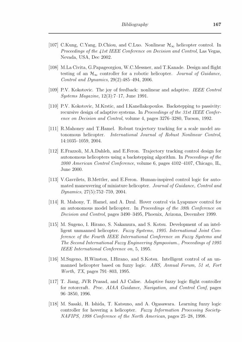
Bibliography 167
[107] C.Kung, C.Yang, D.Chiou, and C.Luo. Nonlinear H∞ helicopter control. In
Proceedings of the 41st IEEE Conference on Decision and Control, Las Vegas,
Nevada, USA, Dec 2002.
[108] M.La Civita, G.Papageorgiou, W.C.Messner, and T.Kanade. Design and flight
testing of an H∞ controller for a robotic helicopter. Journal of Guidance,
Control and Dynamics, 29(2):485–494, 2006.
[109] P.V. Kokotovic. The joy of feedback: nonlinear and adaptive. IEEE Control
Systems Magazine, 12(3):7–17, June 1991.
[110] P.V. Kokotovic, M.Krstic, and I.Kanellakopoulos. Backstepping to passivity:
recursive design of adaptive systems. In Proceedings of the 31st IEEE Confer-
ence on Decision and Control, volume 4, pages 3276–3280, Tucson, 1992.
[111] R.Mahoney and T.Hamel. Robust trajectory tracking for a scale model au-
tonomous helicopter. International Journal of Robust Nonlinear Control,
14:1035–1059, 2004.
[112] E.Frazzoli, M.A.Dahleh, and E.Feron. Trajectory tracking control design for
autonomous helicopters using a backstepping algorithm. In Proceedings of the
2000 American Control Conference, volume 6, pages 4102–4107, Chicago, IL,
June 2000.
[113] V.Gavrilets, B.Mettler, and E.Feron. Human-inspired control logic for auto-
mated maneuvering of miniature helicopter. Journal of Guidance, Control and
Dynamics, 27(5):752–759, 2004.
[114] R. Mahony, T. Hamel, and A. Dzul. Hover control via Lyapunov control for
an autonomous model helicopter. In Proceedings of the 38th Conference on
Decision and Control, pages 3490–3495, Phoenix, Arizona, December 1999.
[115] M. Sugeno, I. Hirano, S. Nakamura, and S. Kotsu. Development of an intel-
ligent unmanned helicopter. Fuzzy Systems, 1995. International Joint Con-
ference of the Fourth IEEE International Conference on Fuzzy Systems and
The Second International Fuzzy Engineering Symposium., Proceedings of 1995
IEEE International Conference on, 5, 1995.
[116] M.Sugeno, H.Winston, I.Hirano, and S.Kotsu. Intelligent control of an un-
manned helicopter based on fuzzy logic. AHS, Annual Forum, 51 st, Fort
Worth, TX, pages 791–803, 1995.
[117] T. Jiang, JVR Prasad, and AJ Calise. Adaptive fuzzy logic flight controller
for rotorcraft. Proc. AIAA Guidance, Navigation, and Control Conf, pages
96–3850, 1996.
[118] M. Sasaki, H. Ishida, T. Katsuno, and A. Ogasawara. Learning fuzzy logic
controller for hovering a helicopter. Fuzzy Information Processing Society-
NAFIPS, 1998 Conference of the North American, pages 25–28, 1998.
168 Bibliography
[119] TGB Amaral and MM Crisostomo. Automatic helicopter motion control using
fuzzy logic. Fuzzy Systems, 2001. The 10th IEEE International Conference on,
2, 2001.
[120] T.G.Amaral, M.M.Crisostomo, and V.F.Pires. Helicopter motion control us-
ing adaptive neuro-fuzzy inference controller. In Proceedings of the IEEE
28th Annual Conference of the Industrial Electronics Society, volume 3, pages
2090–2095, Nov 2002.
[121] B. Kadmiry, P. Bergsten, and D. Driankov. Autonomous helicopter control
using fuzzy gain scheduling. Robotics and Automation, 2001. Proceedings 2001
ICRA. IEEE International Conference on, 3, 2001.
[122] B. Kadmiry and D. Driankov. A fuzzy gain-scheduler for the attitude control
of an unmanned helicopter. Fuzzy Systems, IEEE Transactions on, 12(4):502–
515, 2004.
[123] EN Sanchez, HM Becerra, and CM Velez. Combining fuzzy and PID con-
trol for an unmanned helicopter. Fuzzy Information Processing Society, 2005.
NAFIPS 2005. Annual Meeting of the North American, pages 235–240, 2005.
[124] C. Cavalcante, J. Cardoso, JJG Ramos, and OR Neves. Design and tuning
of a helicopter fuzzy controller. Fuzzy Systems, 1995. International Joint
Conference of the Fourth IEEE International Conference on Fuzzy Systems
and The Second International Fuzzy Engineering Symposium., Proceedings of
1995 IEEE International Conference on, 3:1549 – 1554, March 1995.
[125] C.Phillips, C.L.Karr, and G.Walker. Helicopter flight control with fuzzy logic
and genetic algorithms. Engineering Applications of Artificial Intelligence,
9(2):175–184, 1996.
[126] F. Homann, T.J. Koo, and O. Shakernia. Evolutionary design of a helicopter
autopilot. 3rd On-line World Conf. on Soft Computing (WSC3), 1998.
[127] W.S.McCulloch and W.Pitts. A logical calculus of ideas immanent in nervous
activitiy. Bulletin of Mathematical Biophysics, 5:115–133, 1943.
[128] J.J.Hopfield. Neural networks and physical systems with emergent collective
computational abilities. In Proceedings of the National Academy of Sciences,
pages 2554–2558, 1982.
[129] S.Haykin. Neural Networks: A Comprehensive Foundation. Prentice Hall,
New Jersey, 2nd edition edition, 1999.
[130] R.S.Sutton and A.G.Barto. Reinforcement learning: An introduction. The
MIT Press, Cambridge, Massachusetts, 1998.
[131] D. Rumellhart and J. McClelland, editors. Parallel Distributed Processing.
MIT Press, Cambridge, MA, 1986.
Bibliography 169
[132] A.E.Bryson and Y.C.Ho. Applied Optimal Control. Blaisdell, New York, 1969.
[133] P.J.Werbos. Beyond Regression: New Tools for Prediction and Analysis in the
Behavioral Sciences. PhD thesis, Harvard University, 1974.
[134] M.T. Hagan and M.Menhaj. Training feedforward networks with the mar-
quardt algorithm. IEEE Transactions on Neural Networks, 5(6):989–993,
1994.
[135] The MathWorks, Inc., www.mathworks.com. Neural Network Toolbox User’s
Guide, 2005.
[136] J.F. Montgomery and G.A. Bekey. Learning helicopter control through teach-
ing by showing. In Proceedings of the 37th IEEE Conference on Decision and
Control, volume 4, 1998.
[137] L.X.Wang. Adaptice Fuzzy Systems and Control: Design and Stability Analy-
sis. Prentice-Hall, Englewood Cliffs, NJ, 1994.
[138] D.Y.Maharaj. The Application of Nonlinear Control Theory to Robust Heli-
copter Flight Control. PhD thesis, Department of Aeronautics, Imperial Col-
lege of Science, Technology and Medicine, 1994.
[139] G. Buskey, G. Wyeth, and J.Roberts. Autonomous helicopter hover using
an artificial neural network. In Proceedings 2001 ICRA. IEEE International
Conference on Robotics and Automation, volume 2, pages 1635– 1640, 2001.
[140] J.A.Bagnell and J.G.Schneider. Autonomous helicopter control using rein-
forcement learning policy search methods. In Proceedings of the 2001 IEEE
International Conference on Robotics and Automation, Seoul, Korea, May
2001.
[141] A.Moore and J.Schneider. Memory based stochastic optimization. In Ad-
vances in Neural Information Processing Systems 8, Denver, CO, USA, Nov
1995. MIT Press.
[142] A.Y. Ng, H.J. Kim, M.I. Jordan, and S. Sastry. Autonomous helicopter flight
via reinforcement learning. Advances in Neural Information Processing Sys-
tems, 16, 2004.
[143] A.Y. Ng and M. Jordan. PEGASUS: A policy search method for large MDPs
and POMDPs. In Proceedings of the Sixteenth Conference on Uncertainty in
Artificial Intelligence, pages 406–415, 2000.
[144] A.Y. Ng, A. Coates, M. Diel, V. Ganapathi, J. Schulte, B. Tse, E. Berger, and
E. Liang. Autonomous inverted helicopter flight via reinforcement learning.
International Symposium on Experimental Robotics, 2004.
170 Bibliography
[145] AJ Calise, BS Kim, J. Leitner, and JVR Prasad. Helicopter adaptive flight
control using neural networks. In Proceedings of the 33rd IEEE Conference
on Decision and Control, volume 4, 1994.
[146] B.S.Kim. Nonlinear Flight Control Using Neural Networks. PhD thesis,
School of Aerospace Engineering, Georgia Institute of Technology, Atlanta,
Georgia, USA, Dec 1993.
[147] J. Leitner, A. Calise, and JVR Prasad. A full authority helicopter adaptive
neuro-controller. In Proceedings of the IEEE Aerospace Conference, volume 2,
1998.
[148] J.V.R Prasad, A.J. Calise, J.E.Corban, and Y. Pei. Adaptive nonlinear con-
troller synthesis and flight test evaluation on an unmanned helicopter. In
IEEE International Conference on Control Applications, 1999.
[149] A.J.Calise, H.Lee, and N.Kim. High bandwidth adaptive flight control. In
AIAA Guidance, Navigation and Control Conference, Denver, Colorado, Au-
gust 2000.
[150] N.Hovakimyan, N.Kim, A.J. Calise, and J. V. R. Prasad. Adaptive out-
put feedback for high-bandwidth control of an unmanned helicopter. In
AIAA Guidance, Navigation, and Control Conference, pages 1–11, Montreal,
Canada, 6–9 August 2001.
[151] J.E.Corban, A.J. Calise, J.V.R.Prasad, J.Hur, and N.Kim. Flight evaluation
of adaptive high-bandwidth control methods for unmanned helicopters. In
AIAA Guidance, Navigation and Control Conference, Monterey, CA, August
2002.
[152] J.E.Corban, A.J.Calise, J.V.R.Prasad an G.Heynen, B.Koenig, and J.Hur.
Flight evaluation of an adaptive velocity command system for unmanned heli-
copters. In AIAA Guidance, Navigation, and Control Conference and Exhibit,
Austin, Texas, 11-14 August 2003.
[153] E.N.Johnson and S.K.Kannan. Adaptive trajectory control for autonomous
helicopters. Journal of Guidance, Control and Dynamics, 28(3), 2005.
[154] C.Munzinger. Development of a real-time flight simulator for an experimental
model helicopter. Master’s thesis, Georgia Institute of Technology, Atlanta,
Dec 1998.
[155] R.Cunha and C.Silvestre. SimModHeli: A dynamic simulator for model-scale
helicopters. In 11th Mediterranean Conference on Control and Automation,
Rhodes, Greece, June 2003.
[156] V. Gavrilets, I. Martinos, B. Mettler, and E. Feron. Flight test and simulation
results for an autonomous aerobatic helicopter. In The 21st Proceedings of the
Digital Avionics Systems Conference, volume 2, pages 311–316. IEEE, 2002.
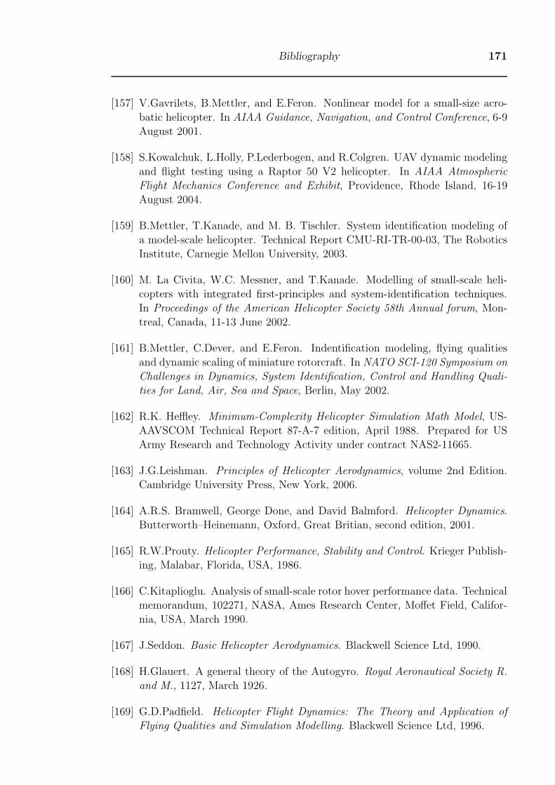
Bibliography 171
[157] V.Gavrilets, B.Mettler, and E.Feron. Nonlinear model for a small-size acro-
batic helicopter. In AIAA Guidance, Navigation, and Control Conference, 6-9
August 2001.
[158] S.Kowalchuk, L.Holly, P.Lederbogen, and R.Colgren. UAV dynamic modeling
and flight testing using a Raptor 50 V2 helicopter. In AIAA Atmospheric
Flight Mechanics Conference and Exhibit, Providence, Rhode Island, 16-19
August 2004.
[159] B.Mettler, T.Kanade, and M. B. Tischler. System identification modeling of
a model-scale helicopter. Technical Report CMU-RI-TR-00-03, The Robotics
Institute, Carnegie Mellon University, 2003.
[160] M. La Civita, W.C. Messner, and T.Kanade. Modelling of small-scale heli-
copters with integrated first-principles and system-identification techniques.
In Proceedings of the American Helicopter Society 58th Annual forum, Mon-
treal, Canada, 11-13 June 2002.
[161] B.Mettler, C.Dever, and E.Feron. Indentification modeling, flying qualities
and dynamic scaling of miniature rotorcraft. In NATO SCI-120 Symposium on
Challenges in Dynamics, System Identification, Control and Handling Quali-
ties for Land, Air, Sea and Space, Berlin, May 2002.
[162] R.K. Heffley. Minimum-Complexity Helicopter Simulation Math Model, US-
AAVSCOM Technical Report 87-A-7 edition, April 1988. Prepared for US
Army Research and Technology Activity under contract NAS2-11665.
[163] J.G.Leishman. Principles of Helicopter Aerodynamics, volume 2nd Edition.
Cambridge University Press, New York, 2006.
[164] A.R.S. Bramwell, George Done, and David Balmford. Helicopter Dynamics.
Butterworth–Heinemann, Oxford, Great Britian, second edition, 2001.
[165] R.W.Prouty. Helicopter Performance, Stability and Control. Krieger Publish-
ing, Malabar, Florida, USA, 1986.
[166] C.Kitaplioglu. Analysis of small-scale rotor hover performance data. Technical
memorandum, 102271, NASA, Ames Research Center, Moffet Field, Califor-
nia, USA, March 1990.
[167] J.Seddon. Basic Helicopter Aerodynamics. Blackwell Science Ltd, 1990.
[168] H.Glauert. A general theory of the Autogyro. Royal Aeronautical Society R.
and M., 1127, March 1926.
[169] G.D.Padfield. Helicopter Flight Dynamics: The Theory and Application of
Flying Qualities and Simulation Modelling. Blackwell Science Ltd, 1996.
172 Bibliography
[170] M.B.Tischler and R.K.Temple. Aircraft and Rotorcraft System Identification:
Engineering Methods with Flight Test Examples. AIAA Education Series, Re-
ston, Virginia, USA, 2006.
[171] A.Cooke and E.W.H.Fitzpatrick. Helicopter Test and Evaluation. AIAA,
2002.
[172] R.Cunha and C.Silvestre. Dynamic modeling and stability analysis of model-
scale helicopters with Bell-Hiller stabilizing bar. In AIAA Guidance Naviga-
tion and Control Conference, Texas, USA, 2003.
[173] M.G.Perhinschi and J.V.R.Prasad. A simulation model of an autonomous
helicopter. In Proceedings of the RPV/UAV 13th Bristol International Con-
ference, pages 36.1–36.13, Bristol, United Kingdom, March 1998.
[174] S.N.Brennan. Modeling and control issues associated with scaled vehicles.
Master’s thesis, Graduate College of the University of Illinois, 1999.
[175] T.R.Beal. Digital simulation of atmospheric turbulence for Dryden and von
Karman models. Journal of Guidance, Control and Dynamics, 16(1), 1993.
[176] J.D.McMinn. Extension of a Kolmogorov atmospheric turbulence model for
time-based simulation implementation. In AIAA Guidance, Navigation, and
Control Conference, pages 322–334, New Orleans, LA, USA, 1997.
[177] Characteristics of atmospheric turbulence near the ground. Technical report,
ESDU, 2001.
[178] Flying qualities of piloted aircraft. Technical Report MIL-F-8785C, United
States Department of Defence, Nov 1980.
[179] M.B.Tischler and M.G.Cauffman. Frequency-response method for rotorcraft
system identification: Flight application to BO-105 coupled rotor/fuselage
dynamics. Journal of the American Helicopter Society, 37(3):3–17, 1992.
[180] B.Mettler, M. B. Tischler, and T.Kanade. System identification modeling of
a small-scale unmanned rotorcraft for flight control design. Journal of the
American Helicopter Society, pages 50–63, January 2002.
[181] TME Inc. Toronto MicroElectronics Inc. - your embedded single board com-
puters. http://www.tme-inc.com/, 2005.
[182] www.slackware.org. The Slackware Linux Project, Oct 2007.
[183] FSM Labs. RTLinux Free. http://www.rtlinuxfree.com/, 2007.
[184] E.N.Johnson and D.P Schrage. The Georgia Tech unmanned aerial research
vehicle: GTMax. In Proceedings of the AIAA Guidance, Navigation, and
Control Conference, Austin, Texas, Aug. 11-14 2003.
Bibliography 173
[185] H. J.Kim, D. H. Shim, and S.Sastry. Flying robots: Modelling, control and
decision making. In Proceedings of the 2002 IEEE International Conference
on Robotics & Automation, pages 66–71, Washington, DC, May 2002.
[186] P.Doherty. Advanced research with autonomous unmanned aerial vehicles. In
Proceedings of the 9th International Conference on Knowledge Representation
and Reasoning, 2004.
[187] J.Charles. CMU’s autonomous helicopter explores new territory. Intelligent
Systems and Their Applications, 13(5):85–87, 1998.
[188] M.Whalley, M.Freed, M.Takahashi, D.Christian, A.Patternson-Hine,
G.Shulein, and R.Harris. The NASA/Army autonomous rotorcraft project.
In Proceedings of the American Helicopter Society 59th Annual Forum, 2003.
[189] Microstrain Inc. MicroStrain: Orientation Sensors. http://www.
microstrain.com/, 2007.
[190] Analog Devices, Inc. Homepage. http://www.analog.com, 2007.
[191] Microchip Technology Inc. Microchip Technology Inc. is a Leading Provided of
Microcontroller and Analaog Semiconductors. http://www.microchip.com,
2007.
[192] M.Dunbabin, S.Brosnan, J.Roberts, and P.Corke. Vibration isolation of au-
tonomous helicopter flight. In Proceedings of the 2004 IEEE International
Conference on Robotics and Automation, New Orleans, LA, April 2004.
[193] NovAtel Inc. GPS Navigation Systems, GPS Tracking Devices: NovAtel Inc.
. http://www.novatel.com, 2007.
[194] Schmitt Measurement Systems Inc. Laser measurement sensors and scanners
- Acuity homepage. http://www.acuitylaser.com/, Oct 2007.
[195] M.A.Garratt, H.Pota, A.Lambert, and S.Eckersley-Maslin. Systems for auto-
mated launch and recovery of an Unmanned Aerial Vehicle from ships at sea.
In Proceedings of the 22nd International UAV Systems Conference, Bristol,
UK, 16-18 April 2007.
[196] O.A.Yakimenko, I.I.Kaminer, W.J.Lentz, and P.A.Ghyzel. Unmanned aircraft
navigation for shipboard landing using infrared vision. IEEE Transactions on
Aerospace and Electronic Systems, 38(4):1181–1200, October 2002.
[197] R.M. Haralick, D. Lee, K. Ottenburg, and M. Nolle. Analysis and solutions
of the three point perspective pose estimation problem. In Proceedings of the
IEEE Computer Society Conference on Computer Vision and Pattern Recog-
nition, pages 592–598, 3-6 June 1991.
[198] S.W. Shepperd. Quaternions from rotation matrix. AIAA J. Guid. Control,
1(3):223–224, May-June 1978.
174 Bibliography
[199] NovAtel Inc. OEM4 Family User Manual - Volume 1: Installation and Oper-
ation, rev. 19 edition, 2005.
[200] GPS position accuracy measures. Application note, NovAtel Inc., 10 Dec 2003.
http://www.novatel.com/support/applicationnotes.htm.
[201] R.Y. Tsai. An efficient and accurate camera calibration technique for 3D
machine vision. In Proceedings of IEEE Conference on Computer Vision and
Pattern Recognition, pages 364–374, Miami Beach, FL, 1986.
[202] R.Y. Tsai. A versatile camera calibration technique for high-accuracy 3D
machine vision metrology using off-the-shelf TV cameras and lenses. IEEE
Journal of Robotics and Automation, RA-3(No. 4):323–344, August 1987.
[203] Milan Sonka, Vaclav Hlava, and Roger Boyle. Image Processing Analysis and
Machine Vision. Brooks/Cole Publishing Company, 1999.
[204] P.R.Kalata. The tracking index: A generalized parameter for α - β and α - β
- γ target trackers. IEEE Transactions of Aerospace and Electronic Systems,
AES-20(2):174–182, March 1984.
[205] J.S.Chahl and M.V.Srinivasan. Reflective surfaces for panoramic imaging.
Applied Optics, 36(31):8275–8285, 1997.
[206] P.Corke. An inertial and visual sensing system for a small helicopter. Journal
of Robotic Systems, 21(2):43–51, 2004.
[207] Y.LeCun. Efficient learning and second-order methods, A tutorial at NIPS
93. In Neural Information Processing Systems Conference, Denver, 1993.
[208] T.F. Coleman and Y. Li. An interior, trust region approach for nonlinear
minimization subject to bounds. SIAM Journal on Optimization, 6:418–445,
1996.
[209] R. E. Kalman. A new approach to linear filtering and prediction problems.
Transactions of the ASME - Journal of Basic Engineering, 82:35–45, 1960.
[210] S.F. Schmidt. Computational techniques in Kalman filtering. In Theory and
Applications of Kalman Filtering, volume 139. AGARDograph, Feb 1970.
[211] R.G.Brown and P.Y.C.Hwang. Introduction to Random Signals and Applied
Kalman Filtering. John Wiley and Sons Inc., 3rd edition, 1997.
[212] P.Zarchan and H.Musoff. Fundamental of Kalman filtering: A practical ap-
proach, volume 190 of Progress in Astronautics and and Aeronautics. AIAA,
USA, 2000.
[213] J.Vaganay, M.J.Aldon, and A.Fournier. Mobile robot attitude estimation by
fusion of inertial data. In Proceedings of the IEEE International Conference
on Robotics and Automation, volume 1, pages 277–282, Atlanta, GA, USA,
May 1993.
Bibliography 175
[214] D.Gebre-Egziabher, G.H.Elkaim, J.D.Powell, and B.W.Parkinson. A gyro-free
quaternion-based attitude determination system suitable for implementation
using low cost sensors. In Proceedings of the IEEE Position, Location and
Navigation Symposium, pages 185–192, San Diego, CA, USA, March 2000.
[215] D.B.Kingston and R.W.Beard. Real-time attitude and position estimation
for small UAVs using low-cost sensors. In AIAA 3rd ”Unmanned Unlimited”
Technical Conference, Workshop and Exhibit, Chicago, Ilinois, USA, 20-23 Sep
2004. AIAA-2004-6488.
[216] E.Baird. Visual Flight Control in the Honeybee. PhD thesis, Research School
of Biological Sciences, Australian National University, Canberra, Australia,
April 2007.
[217] MV Srinivasan, FA Miles, and J. Wallman. Visual Motion and its Role in the
Stabilisation of Gaze. Elsevier, Amsterdam, The Netherlands, 1993.
[218] E.Baird, M.V.Srinivasan, S.Zhang, and A.Cowling. Visual control of flight
speed in honeybees. Journal of Experimental Biology, 208:3895–3905, 2005.
[219] A.Barron and M.V.Srinivasan. Visual regulation of ground speed and head-
wind compensation in freely flying honey bees (apis mellifera l.). Journal of
Experimental Biology, 209:978–984, 2006.
[220] J.M.McMichael and Col. M.S.Francis. Micro air vehicles-toward a new di-
mension in flight. http://www.fas.org/irp/program/collect/docs/mav
auvsi.htm, 1997.
[221] G.L. Barrows and C.Neely. Mixed-mode VLSI optic flow sensors for in-flight
control of a micro air vehicle. In Proceedings of the 45th SPIE Annual Meeting,
San Diego, USA, July 31 - August 4 2000.
[222] G.L. Barrows. Future visual microsensors for mini/micro-UAV applications.
In Proceedings of the 2002 7th IEEE International Workshop on Cellular Neu-
ral Networks and Their Applications, pages 498–506, 2002.
[223] J.C. Zufferey, A. Klaptocz, A. Beyeler, J.D. Nicoud, and Floreano. A 10-gram
microflyer for vision-based indoor navigation. Proceedings of the IEEE/RSJ
International Conference on Intelligent Robots and Systems, 2006.
[224] P.Marks. Float like a robot butterfly. New Scientist, pages 26–27, 14 April
2007.
[225] P.C. Arribas and F.M.H. Macia. FPGA implementation of Santos-Victor op-
tical flow algorithm for real-time image processing: an useful attempt. Pro-
ceedings of SPIE, 5117:23–32, 2003.
[226] J. Diaz, E. Ros, F. Pelayo, EM Ortigosa, and S. Mota. FPGA-based real-time
optical-flow system. IEEE Transactions on Circuits and Systems for Video
Technology, 16(2):274–279, 2006.
176 Bibliography
[227] B.A.Cartwright and T.S.Collet. How honey bees use landmarks to guide their
return to a food source. J.Comp Physiol, 151:521–543, 1983.
[228] B.A.Cartwright and T.S.Collet. Landmark learning in bees. Nature, 295:560,
Feb 1992.
[229] W.Sturzl and J.Zeil. Depth, contrast and view-based homing in outdoor
scenes. Biological Cybernetics, 96:519–531, 2007.
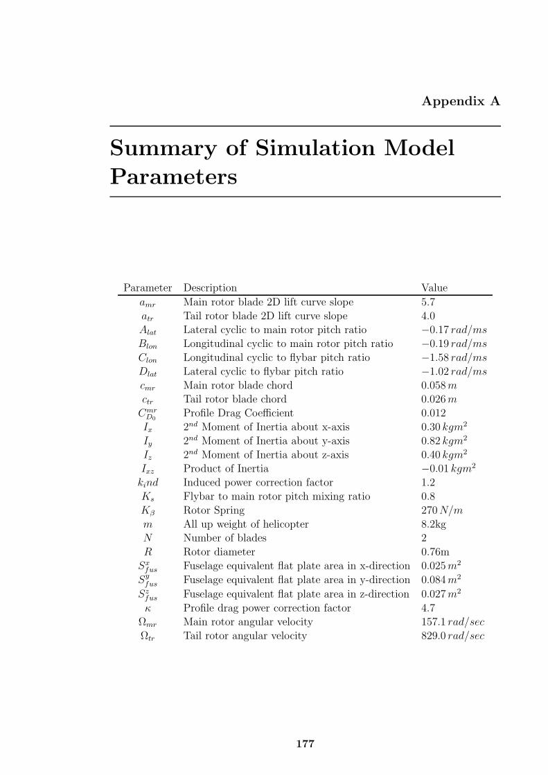
Appendix A
Summary of Simulation Model
Parameters
Parameter Description Value
amr Main rotor blade 2D lift curve slope 5.7
atr Tail rotor blade 2D lift curve slope 4.0
Alat Lateral cyclic to main rotor pitch ratio −0.17 rad/ms
Blon Longitudinal cyclic to main rotor pitch ratio −0.19 rad/ms
Clon Longitudinal cyclic to flybar pitch ratio −1.58 rad/ms
Dlat Lateral cyclic to flybar pitch ratio −1.02 rad/ms
cmr Main rotor blade chord 0.058m
ctr Tail rotor blade chord 0.026m
CmrD0
Profile Drag Coefficient 0.012
Ix 2nd Moment of Inertia about x-axis 0.30 kgm2
Iy 2nd Moment of Inertia about y-axis 0.82 kgm2
Iz 2nd Moment of Inertia about z-axis 0.40 kgm2
Ixz Product of Inertia −0.01 kgm2
kind Induced power correction factor 1.2
Ks Flybar to main rotor pitch mixing ratio 0.8
Kβ Rotor Spring 270N/m
m All up weight of helicopter 8.2kg
N Number of blades 2
R Rotor diameter 0.76m
Sxfus Fuselage equivalent flat plate area in x-direction 0.025m2
Syfus Fuselage equivalent flat plate area in y-direction 0.084m2
Szfus Fuselage equivalent flat plate area in z-direction 0.027m2
κ Profile drag power correction factor 4.7
Ωmr Main rotor angular velocity 157.1 rad/sec
Ωtr Tail rotor angular velocity 829.0 rad/sec
177

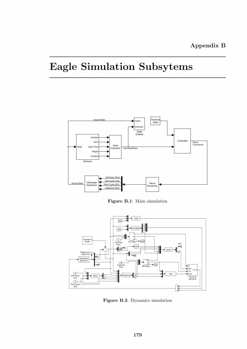
Appendix B
Eagle Simulation Subsytems
StateEstimator
Controller
states
Estimate
StateDisplay
ServoDynamics
State
Inertials
GPS
Optic Flow
Height
Position
Sensors
HelicopterDynamics
DesiredState
emuPitch Cyclic (B1)
Collective Pitch
Actual State
Actual State
EstimatedState
ServoCommands
Tail Rotor Pitch
Roll Cyclic (A1)
Figure B.1: Main simulation
Ptot
1QuaternionState Out
T
Pi
Vi
TR InflowTurbulence
Model
vstab
flybarrotor
flapping
fuselage
power
PiT
ViMR Inflow
Rigid Bodydynamics
[Vitr]
[Vi]
[Vitr]
[Vi]
Ttr
Qmr
Tmr
Rotor
F & M
Forces &Moments
du/dt
emu
emu
emu
emu
emu
emu
emu
4Collective
Pitch
3Pitch Cyclic
(B1)
2Roll Cyclic
(A1)
1Tail Rotor
Pitch
a1b1
Z Mz
cd
Figure B.2: Dynamics simulation
179
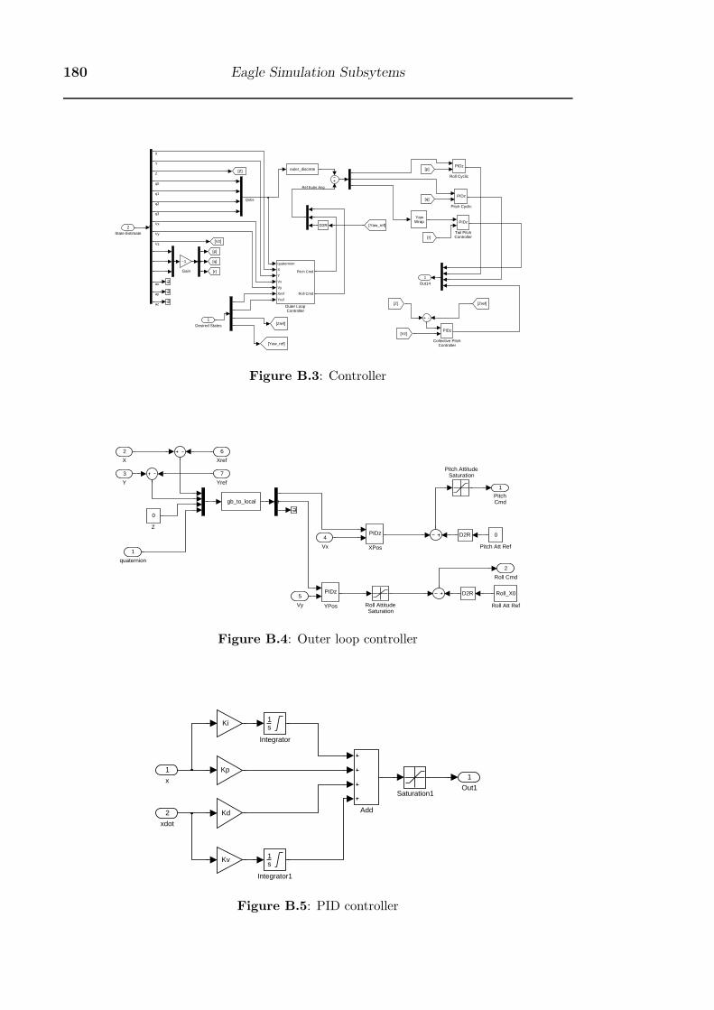
180 Eagle Simulation Subsytems
1
Out14
[r]
[q]
[p]
[Zref]
[Yaw_ref]
[Vz]
[Z]
PIDz
Tail PitchController
YawWrap
euler_discretePIDz
Roll Cyclic
PIDz
Pitch Cyclic
quaternion
X
Y
Vx
Vy
Xref
Yref
Pitch Cmd
Roll Cmd
Outer LoopController
−1
Gain
[Z]
[r]
[Zref]
[Yaw_ref]
[q]
[p]
[Vz]
emu
emu
emu
emu
D2R
PIDz
Collective PitchController
2
State Estimate
1
Desired States
Ref Euler Ang
Qobs
q3
q2
q1
q0
Vz
Vx
Vy
Z
X
Y
ax
ay
az
Figure B.3: Controller
2
Roll Cmd
1
PitchCmd
0
Z
PIDz
YPos
PIDz
XPos
gb_to_local
Roll AttitudeSaturation
Roll_X0
Roll Att Ref
Pitch AttitudeSaturation
0
Pitch Att Ref
emu
D2R
D2R
7
Yref
6
Xref
5
Vy
4
Vx
3
Y
2
X
1
quaternion
Figure B.4: Outer loop controller
1
Out1Saturation1
1s
Integrator1
1s
Integrator
Kv
Ki
Kd
Kp
Add2
xdot
1
x
Figure B.5: PID controller
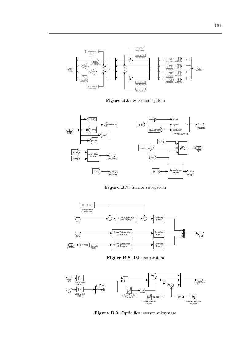
181
1
PWM Out
servo_trim_rud
Trim T/R Pitch
servo_trim_ail
Trim Roll Cyclic
servo_trim_ele
Trim Pitch Cyclic
x’ = Ax+Bu y = Cx+Du
Servo Model3
x’ = Ax+Bu y = Cx+Du
Servo Model2
x’ = Ax+Bu y = Cx+Du
Servo Model1
x’ = Ax+Bu y = Cx+Du
Servo Model
Rate Limiter4
Rate Limiter3
Rate Limiter2
Rate Limiter1Lookup Table
Tail Rotor Pitch
Lookup TableCollective Pitch
1/2500
1/2500
servo_center_ele
Elevator Trim
emuemuemu
servo_trim_col
Collective Pitch Trim
servo_center_ail
Aileron Trim
1
Raw PWM In
Figure B.6: Servo subsystem
5
Position
4
Height
3
Optic Flow
2
GPS
1
Inertials
RangefinderSensor
Optic FlowModel
Accel
Gyros
quaternion
Out1
Inertial Sensors
[uvw]
[XYZ]
[pqr]
[quaternion]
[accel]
GPSModel
[pqr]
[uvw]
[uvw]
[quaternion]
[quaternion]
[XYZ]
[XYZ]
[XYZ] [XYZ]
[accel]
emu1
State
Figure B.7: Sensor subsystem
1
Out1
2 pole Butterworth 20 Hz corner
2 pole Butterworth 10 Hz corner
2 pole Butterworth 20 Hz corner
SamplingErrors
SamplingErrors
SamplingErrors
get_mag
(0 0 g)
Approx InitialConditions
3
quaternion
2
Gyros
1
Accel
MagneticVector
Figure B.8: IMU subsystem
1
Optic Flow
Zero−OrderHold4
Zero−OrderHold2
Uniform RandomNumber5
Uniform RandomNumber1
Uniform RandomNumber
emu
emu
D2R
D2RD2R
2
XYZ
1
uvw
Figure B.9: Optic flow sensor subsystem
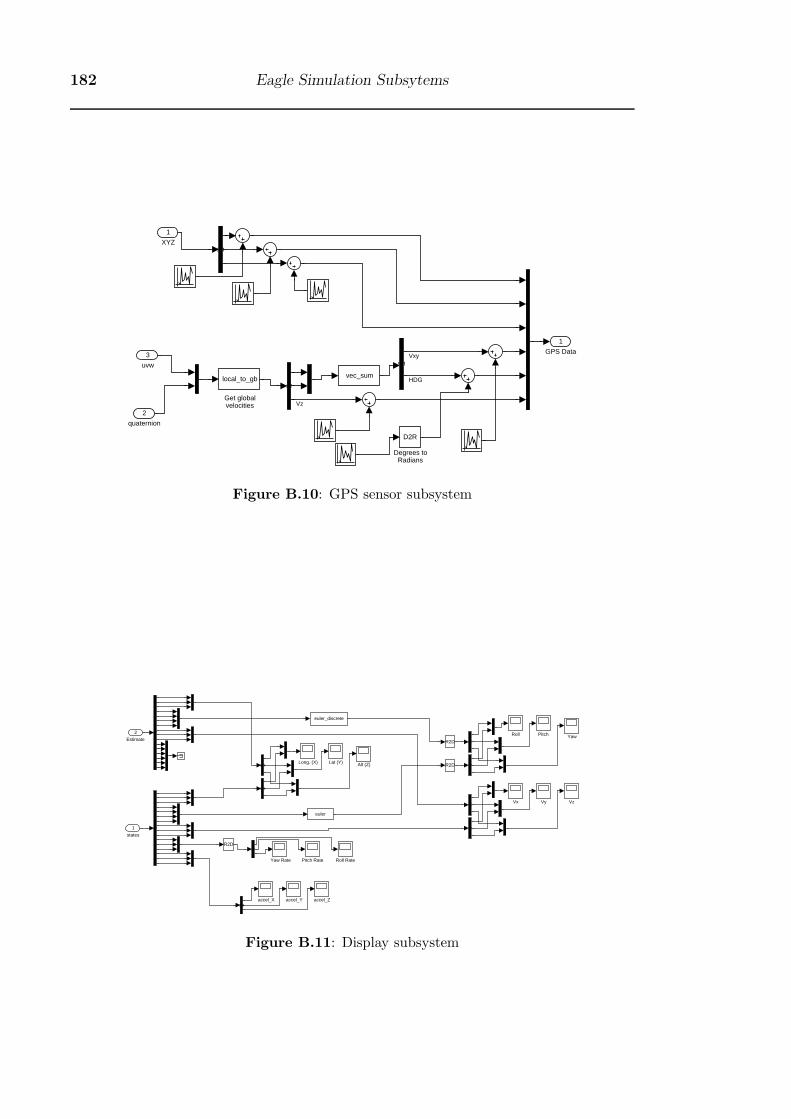
182 Eagle Simulation Subsytems
Get globalvelocities
1
GPS Data
local_to_gb vec_sum
emu
emu
emu
D2R
Degrees toRadians
3
uvw
2
quaternion
1
XYZ
Vxy
Vz
HDG
Figure B.10: GPS sensor subsystem
accel_Zaccel_Yaccel_X
Yaw Rate
Yaw
VzVyVx
euler
euler_discrete
Roll Rate
Roll
R2D
R2D
R2D
Pitch Rate
Pitch
Long. (X) Lat (Y)emu
emu
emu
emu
emu
emu
emu
emu
emu
emu
Alt (Z)
2
Estimate
1
states
Figure B.11: Display subsystem
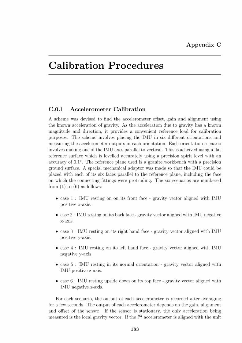
Appendix C
Calibration Procedures
C.0.1 Accelerometer Calibration
A scheme was devised to find the accelerometer offset, gain and alignment using
the known acceleration of gravity. As the acceleration due to gravity has a known
magnitude and direction, it provides a convenient reference load for calibration
purposes. The scheme involves placing the IMU in six different orientations and
measuring the accelerometer outputs in each orientation. Each orientation scenario
involves making one of the IMU axes parallel to vertical. This is acheived using a flat
reference surface which is levelled accurately using a precision spirit level with an
accuracy of 0.1◦. The reference plane used is a granite workbench with a precision
ground surface. A special mechanical adaptor was made so that the IMU could be
placed with each of its six faces parallel to the reference plane, including the face
on which the connecting fittings were protruding. The six scenarios are numbered
from (1) to (6) as follows:
• case 1 : IMU resting on on its front face - gravity vector aligned with IMU
positive x-axis.
• case 2 : IMU resting on its back face - gravity vector aligned with IMU negative
x-axis.
• case 3 : IMU resting on its right hand face - gravity vector aligned with IMU
positive y-axis.
• case 4 : IMU resting on its left hand face - gravity vector aligned with IMU
negative y-axis.
• case 5 : IMU resting in its normal orientation - gravity vector aligned with
IMU positive z-axis.
• case 6 : IMU resting upside down on its top face - gravity vector aligned with
IMU negative z-axis.
For each scenario, the output of each accelerometer is recorded after averaging
for a few seconds. The output of each accelerometer depends on the gain, alignment
and offset of the sensor. If the sensor is stationary, the only acceleration being
measured is the local gravity vector. If the ith accelerometer is aligned with the unit
183
184 Calibration Procedures
vector ζi = ζixi+ ζiy j+ ζizk, then the output Uij of the ith accelerometer for the jth
scenario can be expressed by Equation (C.1).
Uij = kiζi · g= |g|(ζixgjx + ζiygjy + ζizgjz) + Υi (C.1)
where g is the acceleration due to gravity, ki is the accelerometer sensor gain
and Υi is the accelerometer offset.
Since the IMU is placed on a flat surface which is normal to gravity, for each
scenario, only one of gjx, gjy and gjz will be non-zero and equal to unity. This
provides a means of finding the offset for each accelerometer, assuming that the
offset does not change significantly during the calibration. The latter condition can
be enforced by performing the calibration in a constant temperature environment
and allowing the IMU to reach thermal equilibrium from internal heating before the
calibration takes place. Consider the ith accelerometer subject to placement on each
face:
Ui1 = kiζ1x|g| + Υi (C.2)
Ui2 = −kiζ1x|g| + Υi (C.3)
Ui3 = kiζ1y|g| + Υi (C.4)
Ui4 = −kiζ1y|g| + Υi (C.5)
Ui5 = kiζ1z|g| + Υi (C.6)
Ui6 = −kiζ1z|g| + Υi (C.7)
By adding consecutive equations above (e.g. adding Equation (C.2) to (C.3)),
the offset Υi can be found. For better accuracy, the offset can be found from making
use of all of the data as in Equation (C.8).
Υi = (Ui1 + Ui2 + Ui3 + Ui4 + Ui5 + Ui6) /6 (C.8)
The offsets for all accelerometers can be found by repeating the process for each
accelerometer. The gains of each accelerometer can be found next by subtracting
consecutive equations, resulting in Equations (C.2-C.4). For example, subtracting
Equation (C.3) from equation (C.2) eliminates the offset, resulting in Equation
(C.9).
kiζix =Ui1 − Ui2
2|g| (C.9)
kiζiy =Ui3 − Ui4
2|g| (C.10)
kiζiz =Ui5 − Ui6
2|g| (C.11)
185
By squaring both sides of Equations (C.9 - C.11) and then adding the resultant
terms, we arrive at Equation (C.12).
k2i
(a2ix + a2
iy + a2iz
)=
(Ui1 − Ui2
2|g|)2
+
(Ui3 − Ui4
2|g|)2
+
(Ui5 − Ui6
2|g|)2
(C.12)
But since the aij terms are unit vectors, a2ix+a2
iy +a2iz = 1 and thus the gain can
be found from Equation C.13.
ki =
√(Ui1 − Ui2
2|g|)2
+
(Ui3 − Ui4
2|g|)2
+
(Ui5 − Ui6
2|g|)2
(C.13)
Finally the alignment of the accelerometers can be found from Equations (C.9 -
C.11), simply by dividing by the appropriate gains. This leads to the following set
of equations:
ζix =Ui1 − Ui2
2ki|g| (C.14)
ζiy =Ui3 − Ui4
2ki|g| (C.15)
ζiz =Ui5 − Ui6
2ki|g| (C.16)
Once the offset, gain and alignment of the accelerometers have been determined,
the data must be converted into a form that can be used to provide the actual
accelerations from the sensor outputs. In general use, the accelerometer outputs
Ui for the ith accelerometer can be expressed in terms of the actual accelerations
[ax ay az] in matrix form:⎡⎣ U1
U2
U3
⎤⎦ =
⎡⎣ k1ζ1x k1ζ1y k1ζ1zk2ζ2x k2ζ2y k2ζ3zk3ζ3x k3ζ3y k3ζ3z
⎤⎦⎡⎣ axayaz
⎤⎦+
⎡⎣ Υ1
Υ2
Υ3
⎤⎦ (C.17)
Equation (C.17) can be re-arranged to give Equation (C.18) which is imple-
mented on the helicopter to calculate the accelerations. The matrix inversion is
calculated offline as part of the calibration process. Software was written by the
author to prompt the operator through the calibration process and gather the Uijvalues. This software then determines the inverted alignment matrix, offsets (Υi)
and the reciprocal of the gains (1/ki) in a form which can be readily transferred into
non-volatile memory on the helicopter.
⎡⎣ axayaz
⎤⎦ =
⎡⎣ ζ1x ζ1y ζ1zζ2x ζ2y ζ3zζ3x ζ3y ζ3z
⎤⎦−1 ⎡⎣ (U1 − Υ1) /k1
(U2 − Υ2) /k2
(U3 − Υ3) /k3
⎤⎦ (C.18)
186 Calibration Procedures
C.0.2 Gyroscope Calibration
A system was developed by the author for calibrating gyroscopes using an accurate
rotating turntable. A precision rate-of-turn table manufactured by Genisco Tech-
nology Corporation was acquired which is capable of rotation rates between 1o/sec
and 3, 200o/sec with a rate accuracy of 0.1% or 0.05o/sec, whichever is greater. The
calibration procedure determines the gain and alignments of the gyroscopes. The
offset of the gyroscopes is found from a zeroing process on startup, based on the
assumption that the helicopter is not moving when the IMU is first turned on. Dy-
namic estimation of the gyroscope offsets using an EKF is also described in Chapter
8.
The procedure involves fixing the IMU on the turntable and rotating at a number
of known speeds within the range of the sensor. For each speed, several thousand
gyroscope rate samples are recorded and averaged. This process is repeated for each
axis by placing each of three orthogonal faces of the IMU flush with the turntable
plate. Three scenarios are executed:
• case 1 : IMU resting on on its front face - axis of rotation aligned with IMU
positive x-axis.
• case 2 : IMU resting on its right hand face - axis of rotation aligned with IMU
positive y-axis.
• case 3 : IMU resting in its normal orientation - axis of rotation aligned with
IMU positive z-axis.
A line of best fit is made for each gyroscope for the sensor output versus speed.
The slope of the line is the derivative Kij = dUij/d|Ω|. Figure C.1 shows the data
for one axis of the IMU.
The output of each gyroscope depends on the gain and alignment. The gyros are
zeroed before each calibration run to ensure that no offset is present due to thermal
drift. If the ith gyroscope is aligned with the unit vector ζi = ζixi+ ζiyj+ ζizk, then
the slope Kij of the ith gyroscope for the jth scenario can be expressed by Equation
(C.19).
Kij = ki (ζixΩx + ζiyΩy + ζizΩz) (C.19)
where ki is the gain of the gyroscope. Since each IMU face is placed normal to
the axis of rotation, for each scenario, only one of Ωx, Ωy and Ωz will be non-zero
and equal to unity. The slopes for all three gyroscopes for all three scenarios can be
expressed in matrix form as shown in Equation (C.20).⎡⎣ K11 K12 K13
K21 K22 K23
K31 K32 K33
⎤⎦ =
⎡⎣ k1ζ1x k1ζ1y k1ζ1zk2ζ2x k2ζ2y k2ζ2zk3ζ3x k3ζ3y k1ζ3z
⎤⎦ (C.20)
Noting that ζ2ix+ζ
2iy+ζ
2iz = 1, we can now derive the gains from Equation (C.20):
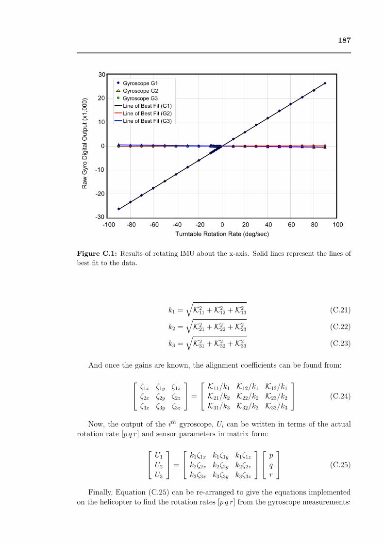
187
-30
-20
-10
0
10
20
30
-100 -80 -60 -40 -20 0 20 40 60 80 100
Turntable Rotation Rate (deg/sec)
Ra
w G
yro
Dig
ita
l O
utp
ut
(x1
,00
0)
Gyroscope G1
Gyroscope G2
Gyroscope G3
Line of Best Fit (G1)
Line of Best Fit (G2)
Line of Best Fit (G3)
Figure C.1: Results of rotating IMU about the x-axis. Solid lines represent the lines of
best fit to the data.
k1 =√
K211 + K2
12 + K213 (C.21)
k2 =√
K221 + K2
22 + K223 (C.22)
k3 =√
K231 + K2
32 + K233 (C.23)
And once the gains are known, the alignment coefficients can be found from:
⎡⎣ ζ1x ζ1y ζ1zζ2x ζ2y ζ2zζ3x ζ3y ζ3z
⎤⎦ =
⎡⎣ K11/k1 K12/k1 K13/k1
K21/k2 K22/k2 K23/k2
K31/k3 K32/k3 K33/k3
⎤⎦ (C.24)
Now, the output of the ith gyroscope, Ui can be written in terms of the actual
rotation rate [p q r] and sensor parameters in matrix form:
⎡⎣ U1
U2
U3
⎤⎦ =
⎡⎣ k1ζ1x k1ζ1y k1ζ1zk2ζ2x k2ζ2y k2ζ2zk3ζ3x k3ζ3y k3ζ3z
⎤⎦⎡⎣ p
q
r
⎤⎦ (C.25)
Finally, Equation (C.25) can be re-arranged to give the equations implemented
on the helicopter to find the rotation rates [p q r] from the gyroscope measurements:
188 Calibration Procedures
⎡⎣ p
q
r
⎤⎦ =
⎡⎣ ζ1x ζ1y ζ1zζ2x ζ2y ζ2zζ3x ζ3y ζ3z
⎤⎦−1 ⎡⎣ U1/k1
U2/k2
U3/k3
⎤⎦ (C.26)
C.0.3 Magnetometer Calibration
The magnetometer parameters to be determined by calibration are offset, sensor gain
and alignment. Unlike gravity, the variation of the magnetic field over the earth’s
surface is significant. Indeed, the earth’s magnetic field vector has a horizontal
and vertical component. The angle between the field vector and vertical is known
as magnetic dip and varies from 0o at the equator to 90o at the North and South
magnetic poles. In the Canberra region, the local magnetic dip is approximately 65◦
such that the magnetic field vector actually has a stronger vertical component than
horizontal component. A primary objective when designing the calibration process
was to develop an algorithm that could be executed without apriori knowledge of the
local magnetic field strength, direction or dip angle. This would simplify the process
and make it less susceptible to unexpected variations in the local field properties.
The procedure developed involves rotating the IMU about each of its three axes
and recording the outputs from each magnetometer for each of the three cases.
The resulting data is in the form of three sine waves for each magnetometer. By
considering the magnitude and DC offset of each sine wave, it is possible to determine
the alignment and gain of each sensor. The calibration apparatus constructed for
magnetometer calibration is shown in Figure C.2. The apparatus consists of a
stepper motor with 400 steps per revolution which drives a mounting pedestal for
the IMU via a long shaft. The stepper motor is controlled through the parallel port
of a PC. The same PC is interfaced to the IMU via an RS232 cable connected to a
spare serial port. The shaft is rotated in steps of 0.9◦ at a time. After each step, a
delay is enforced by the calibration software to allow transients due to the analog
filters to settle. A number of samples are taken at each step for each magnetometer,
averaged and then recorded on the PC. Once data for one complete revolution is
recorded a least squares method is used to fit a sine wave to the data. The amplitude
and DC offset for each sine wave is stored.
The shaft and mounting bracket is made of non-ferrous metals to preserve the
earth’s natural magnetic field properties. Figure C.3 is a graph showing the typical
variation of a single magnetometer as it is rotated about each axis of the IMU.
Calibration is conducted outdoors away from large metal objects, power conductors
and at a minimum height above soil.
We begin our analysis by defining unit vectors i, j, k aligned with the calibration
apparatus rotational axis, such that i is parallel to the axes of the machine, j
is horizontal to the right when looking from the motor side of the device and k
is pointing vertically down in accordance with the right hand rule. The earth’s
magnetic field can then be expressed in terms of components λx, λy and λz along
these unit vector directions:
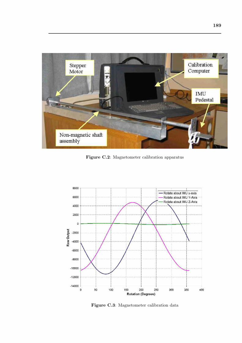
189
Figure C.2: Magnetometer calibration apparatus
Figure C.3: Magnetometer calibration data
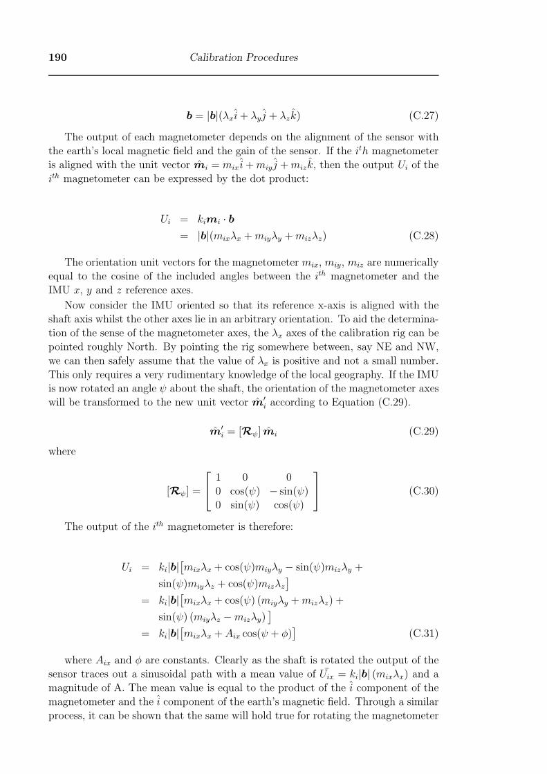
190 Calibration Procedures
b = |b|(λxi+ λy j + λzk) (C.27)
The output of each magnetometer depends on the alignment of the sensor with
the earth’s local magnetic field and the gain of the sensor. If the ith magnetometer
is aligned with the unit vector mi = mix i+miy j +mizk, then the output Ui of the
ith magnetometer can be expressed by the dot product:
Ui = kimi · b= |b|(mixλx +miyλy +mizλz) (C.28)
The orientation unit vectors for the magnetometer mix, miy, miz are numerically
equal to the cosine of the included angles between the ith magnetometer and the
IMU x, y and z reference axes.
Now consider the IMU oriented so that its reference x-axis is aligned with the
shaft axis whilst the other axes lie in an arbitrary orientation. To aid the determina-
tion of the sense of the magnetometer axes, the λx axes of the calibration rig can be
pointed roughly North. By pointing the rig somewhere between, say NE and NW,
we can then safely assume that the value of λx is positive and not a small number.
This only requires a very rudimentary knowledge of the local geography. If the IMU
is now rotated an angle ψ about the shaft, the orientation of the magnetometer axes
will be transformed to the new unit vector m′i according to Equation (C.29).
m′i = [Rψ] mi (C.29)
where
[Rψ] =
⎡⎣ 1 0 0
0 cos(ψ) − sin(ψ)
0 sin(ψ) cos(ψ)
⎤⎦ (C.30)
The output of the ith magnetometer is therefore:
Ui = ki|b|[mixλx + cos(ψ)miyλy − sin(ψ)mizλy +
sin(ψ)miyλz + cos(ψ)mizλz]
= ki|b|[mixλx + cos(ψ) (miyλy +mizλz) +
sin(ψ) (miyλz −mizλy)]
= ki|b|[mixλx + Aix cos(ψ + φ)
](C.31)
where Aix and φ are constants. Clearly as the shaft is rotated the output of the
sensor traces out a sinusoidal path with a mean value of Uix = ki|b| (mixλx) and a
magnitude of A. The mean value is equal to the product of the i component of the
magnetometer and the i component of the earth’s magnetic field. Through a similar
process, it can be shown that the same will hold true for rotating the magnetometer
191
about any of the axes making up the box. Hence for the ith sensor, rotated about
each axis of the box,
Uix = ki|b|mixλx
Uiy = ki|b|miyλx
Uiz = ki|b|mizλx (C.32)
Note that only the component of the magnetic field aligned with the shaft affects
the average value of the output. The shaft axis should therefore be selected to lie
in an orientation which is more parallel than perpendicular to the magnetic field, so
that the magnitude of the results is optimised.
Rearranging components of Equation (C.32),
ki|b|λx =Uixmix
=Uiymiy
=Uizmiz
(C.33)
Inverting,
mix
Uix=miy
Uiy=miz
Uiz(C.34)
Since mix2 +miy
2 +miz2 = 1,
1
mix
=
√1 +
(UiyUix
)2
+
(UizUix
)2
1
miy
=
√1 +
(UixUiy
)2
+
(UizUiy
)2
1
miz
=
√1 +
(UixUiz
)2
+
(UiyUiz
)2
(C.35)
The equations in (C.35) can be used to determine the magnitude of the magne-
tometer unit vectors, but not the sense. Also, numeric difficulties can be experienced
if either Uix, Uiy or Uiz are small numbers. Thus a more robust strategy is to choose
the equation from (C.35) with the largest denominator and use this to find one of
the unit vector magnitudes. Equation (C.33) is then used to find the remaining unit
vectors. The sense of the magnitude can also be found from Equation (C.33) based
on the convention that ki|b|λx is a positive number.
The IMU can be oriented with any of its three axes aligned with the axis of
rotation of the calibration apparatus. The pedestal of the rig has a face which is
normal to the shaft, so that by clamping one of the faces of the IMU flush to the
pedestal, one of the IMU axes can be aligned with the rotational axes. We denote
the magnitude of the varying part of the sine wave as Aix, Aiy, Aiz, for rotations
about the IMU x,y and z axes respectively. The magnitude of the varying part of
Equation (C.31), resulting from rotating the IMU about its x-axis is:
192 Calibration Procedures
A2ix = k2
i |b|2 (miyλy +mizλz)2 + (miyλz −mizλy)
2
= k2i |b|2
(m2iy +m2
iz
) (λ2y + λ2
z
)= ki|b|2
(1 −m2
ix
) (λ2y + λ2
z
)(C.36)
The same derivation applied to each axis in turn results in the following set of
three equations:
A2ix = k2
i |b|2(1 −m2
ix
) (λ2y + λ2
z
)A2iy = k2
i |b|2(1 −m2
iy
) (λ2y + λ2
z
)A2iz = k2
i |b|2(1 −m2
iz
) (λ2y + λ2
z
)(C.37)
The gain ki for each magnetometer may now be calculated by combining Equa-
tions (C.32) and (C.37). Consider first the Equation (C.36) for rotation about the
IMU x-axis:
k2i |b|2
(λ2y + λ2
z
)=
A2ix
1 −m2ix
(C.38)
And from equation C.32:
k2i |b|2λ2
x =
(Uixmix
)2
(C.39)
Adding Equations (C.38) and (C.39),
k2i |b|2
(λ2x + λ2
y + λ2z
)=
(Uixmix
)2
+
(A2ix
1 −m2ix
)(C.40)
Since λ2x + λ2
y + λ2z = 1
ki =1
|b|
√(Uixmix
)2
+
(A2ix
1 −m2ix
)(C.41)
Alternately the gain of each magnetometer can be found from the IMU rotations
about the IMU y and z axes. The resulting Equations are:
ki =1
|b|
√(Uixmix
)2
+
(A2iy
1 −m2iy
)(C.42)
ki =1
|b|
√(Uixmix
)2
+
(A2iz
1 −m2iz
)(C.43)
The final step in the calibration process is to develop a calibration matrix to
convert the raw output of the magnetometers into components of the relative field
vector which are properly aligned with the helicopter body axes. This matrix is
193
found by inverting the matrix of unit vectors and gains. Since the output Ui of the
3 magnetometers is given by,
⎡⎣ U1
U2
U3
⎤⎦ =[k1 k2 k3
] ⎡⎣ m1x m1y m1z
m2x m2y m2z
m3x m3y m3z
⎤⎦⎡⎣ Bx
By
Bz
⎤⎦ = [K]T [M ] b (C.44)
Then the magnetic field vector can be determined from Equation (C.45).⎡⎣ Bx
By
Bz
⎤⎦ =[
1k1
1k2
1k3
] ⎡⎣ m1x m1y m1z
m2x m2y m2z
m3x m3y m3z
⎤⎦−1 ⎡⎣ U1
U2
U3
⎤⎦ (C.45)
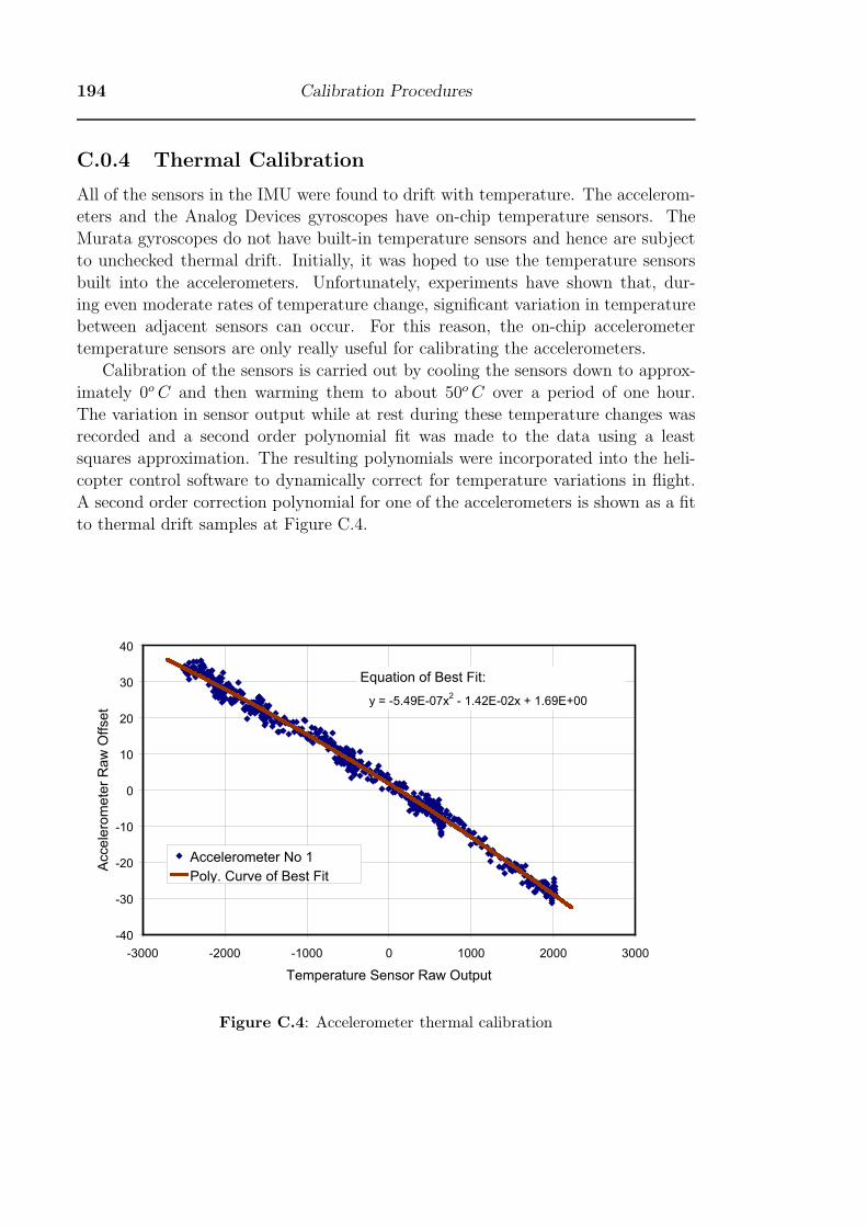
194 Calibration Procedures
C.0.4 Thermal Calibration
All of the sensors in the IMU were found to drift with temperature. The accelerom-
eters and the Analog Devices gyroscopes have on-chip temperature sensors. The
Murata gyroscopes do not have built-in temperature sensors and hence are subject
to unchecked thermal drift. Initially, it was hoped to use the temperature sensors
built into the accelerometers. Unfortunately, experiments have shown that, dur-
ing even moderate rates of temperature change, significant variation in temperature
between adjacent sensors can occur. For this reason, the on-chip accelerometer
temperature sensors are only really useful for calibrating the accelerometers.
Calibration of the sensors is carried out by cooling the sensors down to approx-
imately 0oC and then warming them to about 50oC over a period of one hour.
The variation in sensor output while at rest during these temperature changes was
recorded and a second order polynomial fit was made to the data using a least
squares approximation. The resulting polynomials were incorporated into the heli-
copter control software to dynamically correct for temperature variations in flight.
A second order correction polynomial for one of the accelerometers is shown as a fit
to thermal drift samples at Figure C.4.
y = -5.49E-07x2 - 1.42E-02x + 1.69E+00
-40
-30
-20
-10
0
10
20
30
40
-3000 -2000 -1000 0 1000 2000 3000
Temperature Sensor Raw Output
Acce
lero
me
ter
Ra
w O
ffse
t
Accelerometer No 1
Poly. Curve of Best Fit
Equation of Best Fit:
Figure C.4: Accelerometer thermal calibration
Related Documents