
0199355959
Dec 04, 2015
The game of tennis raises many challenging questions to a statistician
Welcome message from author
This document is posted to help you gain knowledge. Please leave a comment to let me know what you think about it! Share it to your friends and learn new things together.
Transcript


ANALYZING WIMBLEDON
The game of tennis raises many challenging questions to a statisti-cian. Is it true that serving first in a set gives an advantage? Orserving with new balls? Is the seventh game in a set particularly im-portant? Are top players more ‘stable’ than other players? Do realchampions win the big points? These, and many other questions,are formulated as ‘hypotheses’ and tested statistically. This bookdiscusses how the outcome of a match can be predicted (even whilethe match is in progress), which points are important and whichare not, how to choose an optimal service strategy, and whethera ‘winning mood’ actually exists in tennis. Aimed at readers withsome knowledge of mathematics and statistics, the book uses tennis(Wimbledon in particular) as a vehicle to illustrate the power andbeauty of statistical reasoning.
Franc Klaassen is Professor of International Economics at the Uni-versity of Amsterdam. After obtaining masters degrees in econo-metrics and economics and a PhD at Tilburg University, he movedto the University of Amsterdam in 1999. Klaassen is a fellow of theTinbergen Institute and was a visiting fellow at the University ofWisconsin-Madison. His main research interests are the empiricalanalysis of international economics and finance, fiscal policy, andsports, mainly tennis, on which he has published widely. He is anenthusiastic tennis player and, as a junior, was selected to trainwith the Royal Dutch Lawn Tennis Association for nine years.
Jan R. Magnus is Emeritus Professor at Tilburg University andVisiting Professor of Econometrics at the VU University Amster-dam. He studied econometrics and philosophy at the University ofAmsterdam, where he obtained his PhD in Economics. He workedat the Universities of Amsterdam, Leiden, and British Columbia be-fore moving to the London School of Economics in 1981. In 1996 hewas appointed Research Professor of Econometrics at Tilburg Uni-versity. Magnus held visiting positions at University of CaliforniaSan Diego, New Economic School of Moscow, European UniversityInstitute in Florence, and University of Tokyo, among others. Heis author or coauthor of eight books and more than one hundredscientific papers.

This page intentionally left blank

Analyzing Wimbledon
The Power of Statistics
Franc Klaassen
Amsterdam School of Economics,University of Amsterdam, The Netherlands
Jan R. Magnus
Department of Econometrics & Operations Research,VU University Amsterdam, The Netherlands
1

Oxford University Press is a department of the University of Oxford. It furthers theUniversity’s objective of excellence in research, scholarship, and education by
publishing worldwide.
Oxford New YorkAuckland Cape Town Dar es Salaam Hong Kong KarachiKuala Lumpur Madrid Melbourne Mexico City Nairobi
New Delhi Shanghai Taipei Toronto
With offices inArgentina Austria Brazil Chile Czech Republic France GreeceGuatemala Hungary Italy Japan Poland Portugal SingaporeSouth Korea Switzerland Thailand Turkey Ukraine Vietnam
Oxford is a registered trade mark of Oxford University Press in the UKand certain other countries.
Published in the United States of America byOxford University Press
198 Madison Avenue, New York, NY 10016
c© Franc Klaassen and Jan R. Magnus 2014
All rights reserved. No part of this publication may be reproduced, stored in aretrieval system, or transmitted, in any form or by any means, without the prior
permission in writing of Oxford University Press, or as expressly permitted by law,by license, or under terms agreed with the appropriate reproduction rights
organization. Inquiries concerning reproduction outside the scope of the above shouldbe sent to the Rights Department, Oxford University Press, at the address above.
You must not circulate this work in any other form and you must impose this samecondition on any acquirer.
Library of Congress Cataloging-in-Publication DataKlaassen, Franc.
Analyzing Wimbledon: the power of statistics / Franc Klaassen, Jan R. Magnus.pages cm
Includes bibliographical references and index.ISBN 978-0-19-935595-2 (cloth: alk. paper) – ISBN 978-0-19-935596-9 (paperback:
alk. paper) 1. Wimbledon Championships (Wimbledon, London, England) 2.Tennis–Statistics. I. Magnus, Jan R. II. Title.
GV999.K58 2014796.342094212–dc23 2013026355
1 3 5 7 9 8 6 4 2
Typeset by the authorsPrinted in the United States of America on acid-free paper
1

To my parents (FK)
To Eveline de Jong (JM)

This page intentionally left blank

Contents
Preface xiii
Acknowledgements xv
1 Warming up 1
Wimbledon . . . . . . . . . . . . . . . . . . . . . . . . . . 1
Commentators . . . . . . . . . . . . . . . . . . . . . . . . 2
An example . . . . . . . . . . . . . . . . . . . . . . . . . . 3
Correlation and causality . . . . . . . . . . . . . . . . . . 4
Why statistics? . . . . . . . . . . . . . . . . . . . . . . . . 5
Sports data and human behavior . . . . . . . . . . . . . . 6
Why tennis? . . . . . . . . . . . . . . . . . . . . . . . . . 8
Structure of the book . . . . . . . . . . . . . . . . . . . . 9
Further reading . . . . . . . . . . . . . . . . . . . . . . . . 10
2 Richard 13
Meeting Richard . . . . . . . . . . . . . . . . . . . . . . . 13
From point to game . . . . . . . . . . . . . . . . . . . . . 15
The tiebreak . . . . . . . . . . . . . . . . . . . . . . . . . 17
Serving first in a set . . . . . . . . . . . . . . . . . . . . . 18
During the set . . . . . . . . . . . . . . . . . . . . . . . . 20
Best-of-three versus best-of-five . . . . . . . . . . . . . . . 21
Upsets . . . . . . . . . . . . . . . . . . . . . . . . . . . . . 23
Long matches: Isner-Mahut 2010 . . . . . . . . . . . . . . 24
Rule changes: the no-ad rule . . . . . . . . . . . . . . . . 27
Abolishing the second service . . . . . . . . . . . . . . . . 28
Further reading . . . . . . . . . . . . . . . . . . . . . . . . 30

viii Contents
3 Forecasting 33
Forecasting with Richard . . . . . . . . . . . . . . . . . . 34
Federer-Nadal, Wimbledon final 2008 . . . . . . . . . . . . 36
Effect of smaller p . . . . . . . . . . . . . . . . . . . . . . 38
Kim Clijsters defeats Venus Williams, US Open 2010 . . . 40
Effect of larger p . . . . . . . . . . . . . . . . . . . . . . . 41
Djokovic-Nadal, Australian Open 2012 . . . . . . . . . . . 42
In-play betting . . . . . . . . . . . . . . . . . . . . . . . . 44
Further reading . . . . . . . . . . . . . . . . . . . . . . . . 46
4 Importance 49
What is importance? . . . . . . . . . . . . . . . . . . . . . 49
Big points in a game . . . . . . . . . . . . . . . . . . . . . 50
Big games in a set . . . . . . . . . . . . . . . . . . . . . . 52
The vital seventh game . . . . . . . . . . . . . . . . . . . 54
Big sets . . . . . . . . . . . . . . . . . . . . . . . . . . . . 56
Are all points equally important? . . . . . . . . . . . . . . 57
The most important point . . . . . . . . . . . . . . . . . . 58
Three importance profiles . . . . . . . . . . . . . . . . . . 59
Further reading . . . . . . . . . . . . . . . . . . . . . . . . 62
5 Point data 65
The Wimbledon data set . . . . . . . . . . . . . . . . . . . 65
Two selection problems . . . . . . . . . . . . . . . . . . . 67
Estimators, estimates, and accuracy . . . . . . . . . . . . 70
Development of tennis over time . . . . . . . . . . . . . . 72
Winning a point on service unraveled . . . . . . . . . . . . 74
Testing a hypothesis: men versus women . . . . . . . . . . 76
Aces and double faults . . . . . . . . . . . . . . . . . . . . 78
Breaks and rebreaks . . . . . . . . . . . . . . . . . . . . . 80
Are our summary statistics too simple? . . . . . . . . . . 82
Further reading . . . . . . . . . . . . . . . . . . . . . . . . 82
6 The method of moments 85
Our summary statistics are too simple . . . . . . . . . . . 85
The method of moments . . . . . . . . . . . . . . . . . . . 88
Enter Miss Marple . . . . . . . . . . . . . . . . . . . . . . 90
Re-estimating p by the method of moments . . . . . . . . 90
Men versus women revisited . . . . . . . . . . . . . . . . . 91

Contents ix
Beyond the mean: variation over players . . . . . . . . . . 92
Reliability of summary statistics: a rule of thumb . . . . . 94
Filtering out the noise . . . . . . . . . . . . . . . . . . . . 97
Noise-free variation over players . . . . . . . . . . . . . . . 99
Correlation between opponents . . . . . . . . . . . . . . . 100
Why bother? . . . . . . . . . . . . . . . . . . . . . . . . . 102
Further reading . . . . . . . . . . . . . . . . . . . . . . . . 102
7 Quality 105
Observable variation over players . . . . . . . . . . . . . . 105
Ranking . . . . . . . . . . . . . . . . . . . . . . . . . . . . 107
Round, bonus, and malus . . . . . . . . . . . . . . . . . . 112
Significance, relevance, and sensitivity . . . . . . . . . . . 114
The complete model . . . . . . . . . . . . . . . . . . . . . 115
Winning a point on service . . . . . . . . . . . . . . . . . 116
Other service characteristics . . . . . . . . . . . . . . . . . 119
Aces and double faults . . . . . . . . . . . . . . . . . . . . 121
Further reading . . . . . . . . . . . . . . . . . . . . . . . . 123
8 First and second service 127
Is the second service more important than the first? . . . 127
Differences in service probabilities explained . . . . . . . . 130
Joint analysis: bivariate GMM . . . . . . . . . . . . . . . 132
Four service dimensions . . . . . . . . . . . . . . . . . . . 134
Four-variate GMM . . . . . . . . . . . . . . . . . . . . . . 134
Further reading . . . . . . . . . . . . . . . . . . . . . . . . 136
9 Service strategy 137
The server’s trade-off . . . . . . . . . . . . . . . . . . . . . 137
The y-curve . . . . . . . . . . . . . . . . . . . . . . . . . . 139
Optimal strategy: one service . . . . . . . . . . . . . . . . 140
Optimal strategy: two services . . . . . . . . . . . . . . . 141
Existence and uniqueness . . . . . . . . . . . . . . . . . . 142
Four regularity conditions for the optimal strategy . . . . 143
Functional form of y-curve . . . . . . . . . . . . . . . . . . 145
Efficiency defined . . . . . . . . . . . . . . . . . . . . . . . 146
Efficiency of the average player . . . . . . . . . . . . . . . 147
Observations for the key probabilities: Monte Carlo . . . 148
Efficiency estimates . . . . . . . . . . . . . . . . . . . . . . 149

x Contents
Mean match efficiency gains . . . . . . . . . . . . . . . . . 150
Efficiency gains across matches . . . . . . . . . . . . . . . 151
Impact on the paycheck . . . . . . . . . . . . . . . . . . . 152
Why are players inefficient? . . . . . . . . . . . . . . . . . 153
Rule changes . . . . . . . . . . . . . . . . . . . . . . . . . 154
Serving in volleyball . . . . . . . . . . . . . . . . . . . . . 155
Further reading . . . . . . . . . . . . . . . . . . . . . . . . 157
10 Within a match 161
The idea behind the point model . . . . . . . . . . . . . . 161
From matches to points . . . . . . . . . . . . . . . . . . . 162
First results at point level . . . . . . . . . . . . . . . . . . 164
Simple dynamics . . . . . . . . . . . . . . . . . . . . . . . 165
The baseline model . . . . . . . . . . . . . . . . . . . . . . 171
Top players and mental stability . . . . . . . . . . . . . . 173
Lessons from the baseline model . . . . . . . . . . . . . . 177
New balls . . . . . . . . . . . . . . . . . . . . . . . . . . . 177
Further reading . . . . . . . . . . . . . . . . . . . . . . . . 180
11 Special points and games 183
Big points . . . . . . . . . . . . . . . . . . . . . . . . . . . 183
Big points and the baseline model . . . . . . . . . . . . . 186
Serving first revisited . . . . . . . . . . . . . . . . . . . . . 187
The toss . . . . . . . . . . . . . . . . . . . . . . . . . . . . 190
Further reading . . . . . . . . . . . . . . . . . . . . . . . . 192
12 Momentum 193
Streaks, the hot hand, and winning mood . . . . . . . . . 193
Why study tennis? . . . . . . . . . . . . . . . . . . . . . . 195
Winning mood in tennis . . . . . . . . . . . . . . . . . . . 196
Breaks and rebreaks . . . . . . . . . . . . . . . . . . . . . 198
Missed breakpoints . . . . . . . . . . . . . . . . . . . . . . 201
The encompassing model . . . . . . . . . . . . . . . . . . 203
The power of statistics . . . . . . . . . . . . . . . . . . . . 204
Further reading . . . . . . . . . . . . . . . . . . . . . . . . 205
13 The hypotheses revisited 207
1 Winning a point on service is an iid process . . . . . 207
2 It is an advantage to serve first in a set . . . . . . . 208

Contents xi
3 Every point (game, set) is equally important toboth players . . . . . . . . . . . . . . . . . . . . . . . 209
4 The seventh game is the most important game inthe set . . . . . . . . . . . . . . . . . . . . . . . . . . 210
5 All points are equally important . . . . . . . . . . . 210
6 The probability that the service is in is the same inthe men’s singles as in the women’s singles . . . . . . 211
7 The probability of a double fault is the same inthe men’s singles as in the women’s singles . . . . . . 211
8 After a break the probability of being broken backincreases . . . . . . . . . . . . . . . . . . . . . . . . . 212
9 Summary statistics give a precise impression of aplayer’s performance . . . . . . . . . . . . . . . . . . 213
10 Quality is a pyramid . . . . . . . . . . . . . . . . . . 213
11 Top players must grow into the tournament . . . . . 215
12 Men’s tennis is more competitive than women’stennis . . . . . . . . . . . . . . . . . . . . . . . . . . 215
13 A player is as good as his or her second service . . . 216
14 Players have an efficient service strategy . . . . . . . 217
15 Players play safer at important points . . . . . . . . 217
16 Players take more risks when they are in a winningmood . . . . . . . . . . . . . . . . . . . . . . . . . . 218
17 Top players are more stable than others . . . . . . . 218
18 New balls are an advantage to the server . . . . . . . 219
19 Real champions win the big points . . . . . . . . . . 220
20 The winner of the toss should elect to serve . . . . . 220
21 Winning mood exists . . . . . . . . . . . . . . . . . . 220
22 After missing breakpoint(s) there is an increasedprobability of being broken in the next game . . . . 221
Appendix A: Tennis rules and terms 223
Tennis rules . . . . . . . . . . . . . . . . . . . . . . . . . . 223
Tennis terms . . . . . . . . . . . . . . . . . . . . . . . . . 224
Appendix B: List of symbols 227
Winning probabilities . . . . . . . . . . . . . . . . . . . . 227
Score probabilities and importance . . . . . . . . . . . . . 228
Service probabilities . . . . . . . . . . . . . . . . . . . . . 228
Quality . . . . . . . . . . . . . . . . . . . . . . . . . . . . 228

xii Contents
Operators . . . . . . . . . . . . . . . . . . . . . . . . . . . 229Miscellaneous variables . . . . . . . . . . . . . . . . . . . . 229Random/unexplained parts . . . . . . . . . . . . . . . . . 229Parameters . . . . . . . . . . . . . . . . . . . . . . . . . . 229Miscellaneous symbols . . . . . . . . . . . . . . . . . . . . 230
Appendix C: Data, software, and mathematicalderivations 231Data . . . . . . . . . . . . . . . . . . . . . . . . . . . . . . 231Software: program Richard . . . . . . . . . . . . . . . . . 232Mathematical derivations . . . . . . . . . . . . . . . . . . 234
Bibliography 237
Index 247

Preface
This is a book about tennis and about statistics. It is possible— as some of our friends predict — that tennis enthusiasts willfind the statistics incomprehensible and that statisticians will notbe interested in tennis. We hope that our friends are mistaken andthat instead the book will encourage people interested in tennisto learn more about tennis and (as a bonus) learn some statistics.We also hope that people with some knowledge of statistics will seehow statistical modeling and analysis can be applied to questions intennis, thus learning more about statistics and (as a bonus) abouttennis.
Our own interest in tennis as a field of statistical study startedmore than fifteen years ago, when watching Wimbledon on televi-sion and listening to the commentators. We collected more thantwenty statements often made by commentators, such as: it is anadvantage to serve first in a set, the seventh game is the most im-portant game in the set, a player is as good as his or her secondservice, new balls are an advantage to the server, and real cham-pions win the big points. After obtaining the necessary data fromIBM, the Official Technology Partner of Wimbledon since 1990, weanalyzed these statements and found many to be false. At thatpoint, our analysis was not sophisticated and our interest was onlyhalf-serious.
Reflecting more on the possibilities of tennis data, we set our-selves the task of answering four questions: (a) which of the hy-potheses on tennis are true and which are not?, (b) do players playevery point as it comes, or are they affected by the past (winningmood) and by characteristics of the current point?, (c) how can

xiv Preface
we forecast who wins a match, not only at the beginning but alsoduring the match?, and (d) is there an optimal service strategyand how close are professional players to this optimal strategy?We answered the first question in Magnus and Klaassen (1999a,b,c;2008) and the other three questions in Klaassen and Magnus (2001,2003a, 2009). Our work appeared in newspapers, tennis magazines,and scientific journals, thus catering to a variety of audiences andrequiring a presentation of the material at different levels.
For an academic to study tennis or some other sport may requirea defense or at least an explanation. We offer no defense of ourinterest in tennis. We could argue (and we shall expand on thislater) that sport statistics as a discipline is useful, because the dataare clean and tell us something about human behavior. But thetruth of the matter is that we only discovered this later and thatwe would have studied tennis even if such additional benefits hadbeen absent.
We can, however, explain why we wrote this book. Our first aimwas to combine the material that we had discussed in our previouspapers with many new results, all within one framework suitable fora specific audience, going slowly from simple to more sophisticated.Our second aim was to show that statistics, when applied carefully,can provide insights that cannot be obtained otherwise; in otherwords, to demonstrate the power of statistics.
The typical reader we have in mind has some knowledge of andinterest in mathematics and statistics, for example at the level ofa third- or fourth-year undergraduate in the US college system,and of course some interest in tennis. The book should also be ofinterest to tennis enthusiasts with less mathematical background.Chapter 13 (the final chapter) is written especially for this audience.It can be read separately from the rest of the book and contains nomathematics.
We hope that our book will prove useful for teaching studentsthe power and scope (and the limitations) of statistics, will pro-vide new insights to tennis enthusiasts and commentators, and willeven tell readers something about human behavior more generally.If we inspire the reader to share at least some of our enthusiasmfor tennis or statistics or both, then we shall consider our missionaccomplished.
Amsterdam, September 2013

Acknowledgements
We are grateful to IBM UK and The All England Lawn Tennisand Croquet Club at Wimbledon for their kindness in providingus with Wimbledon data at point level. Without this initial dataset, there would have been no project, no papers, and no book. Inaddition, we were given summary statistics for all four grand slamtournaments, and we thank IBM UK and the International TennisFederation for their kind cooperation.
Although most of the material in this book has been rethoughtand recalculated, we have drawn freely on our earlier publications.We are grateful to the following publishers, associations, and soci-eties for permission to use material published earlier by us in theirjournals: Kwantitatieve Methoden, Psychologie, Royal StatisticalSociety (The Statistician), Taylor & Francis Ltd. (Journal of Ap-plied Statistics), American Statistical Association (Journal of theAmerican Statistical Association), European Journal of OperationalResearch, Medicine and Science in Tennis, AENORM, MediumEconometrische Toepassingen (MET), STAtOR, Tennis Magazine,and Journal of Econometrics.
Other work appeared earlier in a conference volume of the In-ternational Statistical Institute (ISI) Meetings in Istanbul (1997),and as chapters in the following three books: Tennis Science &Technology (Eds S.J. Haake and A. Coe), Blackwell Science, Ox-ford; Tennis Science & Technology 2 (Ed S. Miller), InternationalTennis Federation, London; and Statistical Thinking in Sports (EdsJ. Albert and R.H. Koning), Chapman & Hall/CRC Press, BocaRaton, FL. We thank the publishers for permission to use materialfrom these chapters in the current book.

xvi Acknowledgements
Much thanks are due to Josette Janssen for editorial assistance,to Jozef Pijnenburg for helping us with the layout and answer-ing all our LATEX questions, to Eveline de Jong for her invaluablehelp to transform Chapter 13 into a palatable text for the non-mathematical reader, and to three exceptionally knowledgable andsympathetic anonymous reviewers.
Almost twenty years have passed since we started this projectin 1994. During this time we talked to many people, attended work-shops, gave presentations, and received anonymous referee reports.Our work has greatly benefitted from the constructive commentsand knowledge of colleagues and friends, and we thank in particu-lar: Roel Beetsma, Jan Boone, Maurice Bun, Erwin Charlier, Ericvan Damme, Tijmen Daniels, Dmitry Danilov, George Deltas, BasDonkers, Martin Dufwenberg, Kees Jan van Garderen, Ronald vanGelder, Noud van Giersbergen, Wouter den Haan, Harry Huizinga,Masako Ikefuji, Henk Jager, Frank de Jong, Philip Jung, FrankKleibergen, Ruud Koning, Siem Jan Koopman, Knox Lovell, CarlMorris, Theo Offerman, Geoff Pollard, Thijs ten Raa, Ward Romp,Arthur van Soest, Keith Sohl, Joep Sonnemans, Mark Steel, KoenVermeylen, Tom Wansbeek, Alan Woodland, Arnold Zellner, andKatia Zhuravskaya. We have been fortunate indeed to have suchsupportive colleagues.

1Warming up
Suppose you are watching a tennis match between Novak Djokovicand Roger Federer. The commentator says: ‘Djokovic serves firstin the set, so he has an advantage’. Why would this be the case?Perhaps because he is then ‘always’ one game ahead, thus creatingmore pressure on the opponent. But does it actually influence himand, if so, how? Now we come to the seventh game, according tosome the most important game in the set. But is it? Federer servesan ace at breakpoint down (30-40). Of course! Real champions winthe big points. But they win most points on service anyway, includ-ing the unimportant points. Do the real champions outperform onbig points or do weaker players underperform, so that it only seemsthat the champions outperform? (The latter will turn out to bethe case.) Then Djokovic serves with new balls, assumed to be anadvantage. But is it really? Next, Federer wins three consecutivegames. He is in a winning mood, the momentum is on his side. Butdoes a ‘winning mood’ actually exist in tennis? All these questions,and many more, will be discussed in this book.
Wimbledon
Vulcanized rubber balls that bounce well on grass were not availableuntil around 1870, and they were a necessary ingredient for theinvention of lawn tennis (played outside), which was based on thethen existing game of ‘real tennis’ (played inside). The inventionis usually attributed to Major Walter C. Wingfield, who patentedhis new recreation in 1874 and called it ‘sphairistike’, an ancientGreek term meaning ‘skill of playing with a ball’. The name was

2 Analyzing Wimbledon
never popular, not least because only those few people well versedin ancient Greek knew how to say it. Luckily, Major Wingfield alsocalled his new recreation ‘lawn tennis’, and this immediately caughton.
The All England Croquet Club at Wimbledon was founded inthe Summer of 1868. Lawn tennis was first played at the club in1875, when one lawn was set aside for this purpose. In 1877 the clubwas retitled The All England Croquet and Lawn Tennis Club. In1882, croquet was dropped from the name, as tennis had becomethe main activity of the club, but in 1889 it was restored to theclub’s name for sentimental reasons, and the club’s name becameThe All England Lawn Tennis and Croquet Club.
The first tennis championship was held in July 1877 (men’s sin-gles only) with twenty-two players. Spencer Gore became the firstchampion and won the Silver Challenge Cup and twelve guineas, nosmall sum (about £800 or $1240 in today’s value), but rather lessthan the £1,150,000 ($1,785,000) that each of the 2012 championsRoger Federer and Serena Williams received.
In 1884 the women’s singles event was held for the first time.Thirteen players entered this competition and Maud Watson be-came the first women’s champion, receiving twenty guineas anda silver flower basket. (William Renshaw, the 1884 men’s singleschampion, received thirty guineas.)
For more than a century The Championships at Wimbledonhave been the most important event on the tennis calendar. Cur-rently 128 men and 128 women participate in the main draw ofthe men’s and women’s singles, competing over seven rounds. Es-pecially because of television broadcasts, tennis is no longer onlya recreation, but has become a sport viewed by millions of peopleall over the world. And everybody has ideas about tennis: players,viewers, journalists, and television commentators.
Commentators
Tennis is one of the most difficult sports to commentate on. Infootball the commentator can provide the name of the player inball possession. In snooker the commentator can suggest possiblesolutions to the problem on the table. In running and swimmingthere is a continuum of time in which the event takes place, maybe
Warming up 3
short (ten seconds), maybe long (two hours), but uninterrupted.
In a tennis match, all these advantages are absent. To providethe name of the player hitting the ball is ridiculous, to mention thescore is often redundant, to make technical comments can occasion-ally be illuminating, but the most serious problem is that most ofthe time nothing happens.
In a men’s singles tennis match at Wimbledon, one point lastsabout five seconds. One game takes about six points, or thirtyseconds. One set takes about ten games, or five minutes. And thematch may take four sets, or twenty minutes. In reality, the matchdoes not take twenty minutes but perhaps three hours. Only 10%of viewing time is taken up by actual play; the rest of the time mustbe filled by the commentator.
This is no easy job. But the job is lightened when the commen-tator can rely on a number of ‘idees recues’, commonly acceptedideas: for example that serving with new balls provides an advan-tage, that a ‘winning mood’ exists, or that top players must ‘growinto the tournament’ and that they perform particularly well at the‘big’ points. Some of these ideas are true but many of them arefalse, and one of the purposes of this book is to decide which ofthese idees recues are true and which are not.
An example
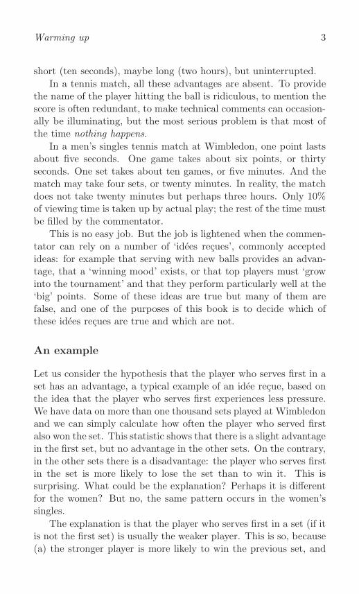
Let us consider the hypothesis that the player who serves first in aset has an advantage, a typical example of an idee recue, based onthe idea that the player who serves first experiences less pressure.We have data on more than one thousand sets played at Wimbledonand we can simply calculate how often the player who served firstalso won the set. This statistic shows that there is a slight advantagein the first set, but no advantage in the other sets. On the contrary,in the other sets there is a disadvantage: the player who serves firstin the set is more likely to lose the set than to win it. This issurprising. What could be the explanation? Perhaps it is differentfor the women? But no, the same pattern occurs in the women’ssingles.
The explanation is that the player who serves first in a set (if itis not the first set) is usually the weaker player. This is so, because(a) the stronger player is more likely to win the previous set, and

4 Analyzing Wimbledon
(b) the previous set is more likely won by serving the set out thanby breaking serve. Therefore, the stronger player typically wins theprevious set on service, so that the weaker player serves first in thenext set. The weaker player is more likely to lose the current setas well, not because of a service (dis)advantage, but because he orshe is the weaker player.
This example shows that we must be careful when we try todraw conclusions based on simple statistics. In this case, the factthat the player who serves first in the second and subsequent setsoften loses the set is true, but this concerns weaker players while thehypothesis concerns all players. If we wish to answer the questionof whether serving first causes a (dis)advantage, we have to controlfor quality differences. If we do this correctly, then we find thatthere is no advantage or disadvantage for the player who servesfirst in a set; in other words, it does not matter who serves first inthe second or subsequent sets. But in the first set it does matter(we’ll see later why), so it is wise to elect to serve after winning thetoss.
But how should we account for differences in quality? The play-ers’ positions on the world-ranking lists obviously give an indication.But how good is this indication? And there are also other aspectsof quality — such as ‘form of the day’ — which are not capturedby the ranking and cannot even be observed. How do we accountfor these? All these issues will be dealt with in this book.
Correlation and causality
In dealing with these and other questions we need to know a lit-tle about statistics. Statistics does not have a good reputation.Many people agree with Mark Twain’s phrase ‘lies, damned lies,and statistics’. One well-known cause of ridicule is the confusion be-tween correlation and causality. There is a high correlation betweeneating much garlic (as in Greece, Italy, and Portugal) and havinga high government budget deficit. Maybe eating garlic causes thedeficit? A new law forbidding garlic consumption would then solvethe current economic crisis. There is also a high correlation betweenreading skills of children and their shoe size, but it would be haz-ardous to conclude that children with big feet are more intelligent.
There are many types of fallacies associated with correlation:

Warming up 5
for example reverse causation (the more firemen are fighting a fire,the bigger the fire is likely to be — hence, more firemen causebigger fires) and common cause (reading skills and shoe size foryoung children have a common cause, namely the age of the child).
Sometimes correlation is a coincidence. If we consider manydata series, then some will be correlated without any common cause.Apparently, near-perfect correlation exists between the death ratein Hyderabad, India, from 1911 to 1919, and variations in the mem-bership of the International Association of Machinists during thesame period. But this does not imply a causal relationship.
All these examples are based on statistics. Using data on garlicconsumption and budget deficits, we do find a positive correlation.This is not a mistake; it is a true reflection of what the data tell us.The mistake lies in the confusion between correlation and causality,and, more generally, in a poor understanding of how statistics canhelp us to understand the world. We should not blame statisticswhen someone suggests solving the economic crisis by forbiddinggarlic consumption. We should blame the ignorance of the personwho suggests this.
Why statistics?
In this book we hope to demonstrate that, while bad use of statisticscan provide misleading and incorrect answers, good use of statisticscan help to clarify phenomena and thus provides important tools formaking decisions in uncertain situations. The previous examples,including the possible (dis)advantage of serving first in a set, showthat using correct statistics in an incorrect way produces incorrectconclusions. This book will provide more examples of this incorrectuse of statistics in tennis, but its main focus will be to show howto use statistics correctly, leading to credible conclusions.
The word ‘statistics’ has two meanings. One meaning is a col-lection of data characteristics, usually averages, as produced by adata-collecting agency such as a national statistical office. Thesestatistics would include information about how tall people are, lifeexpectancy, fertility rates, and so on, and they are called descriptivestatistics.
A second meaning is the mathematical science pertaining tothe collection, analysis, interpretation, and presentation of data.

6 Analyzing Wimbledon
It is this meaning that we are primarily interested in, because itprovides the tools needed to analyze data — for example the toolsto distinguish causality from correlation. This second type is calledmathematical statistics.
Statistics on tennis typically include such items as how oftena player who serves first in a set also wins the set, the numberof double faults, and the percentage of first serves in. These aredescriptive statistics, and they are useful ingredients. Our interest,however, is not in the descriptive statistics themselves, but in whatwe can learn from them. This learning process involves differenttypes of analysis based on mathematical statistics, and we shalldevelop and use more and more sophisticated methods as we goalong.
Mathematical statistics also provides insights that go beyondwhat we infer directly from the data. When only few data areavailable we need to make more assumptions; that is, we need astronger model. Consider, for example, the epic match at Wimble-don 2010, where John Isner defeated Nicolas Mahut 70-68 in thefinal set. This match is unique — there is no match like it in anytennis data set. Still, we can build a realistic model and calcu-late precisely how exceptional the match was. A second example isforecasting the winner of a match while the match is in play. Un-der appropriate and realistic assumptions, credible forecasts can beobtained.
Sports data and human behavior
Studying sports is not only of interest to those interested in sports.There is a second (some would say a first) interest, namely the studyof human behavior. In (professional) sports the players’ objectivesare clear: they want to win. The incentives to win are strong andthe players are highly trained. In everyday life, people differ muchmore. Some pupils are eager to score high grades at school, whileothers just want to pass with minimal effort. Employees in a firmhave different tasks and they differ in terms of experience. Manyof these differences are difficult to observe, thus hampering accu-rate inference in psychology, economics, and related disciplines. Insports analysis there is less unobserved heterogeneity, thus allowingmore accurate inference.
Warming up 7
Moreover, sports data are clean — there are few errors in thedata — and the data collection is transparent and can be checked.Data in economics, psychology, and many other sciences are oftenmessy and ambiguous. To work with clean data provides a greatopportunity for scientists in these fields, and a welcome change fromnormal practice. If results do not come out the way they ‘should’,then this cannot be blamed on the (clean) data. There must be a‘real’ explanation and we have to find it. Maybe our preconceivedidea is wrong or maybe we have not applied the correct statisticalmethod.
Given the abundance of clean sports data we can try and studyhuman behavior in an indirect way. Let us give three examples.Suppose we wish to study whether judges and juries are influencedby social pressure. Useful data from the law courts are not available,so we cannot directly study the possibility of favoritism in the courtsof law under social pressure. But we can study favoritism indirectlyby considering football (soccer) matches and asking whether refer-ees favor the home team, for example by shortening matches inwhich the home team is one goal ahead and lengthening matches inwhich the home team is one goal behind at the end of regular time.It turns out that referees tend to do this, thus favoring the hometeam.
A second example is the question of whether people becomemore cautious when pressure mounts. This too can be analyzed in-directly using sports data. In tennis, some points are more impor-tant than others. Do players behave differently at the key points?They do: they play safer at important points. This teaches ussomething about human behavior, and may have implications out-side tennis, for example in economics. If salaries of agents workingin the financial sector contain not only a bonus but also a sub-stantial malus component, then the consequences of their activitiesmatter in both directions (like winning or losing a tennis match).The behavior of professional tennis players suggests that financialagents will then pursue safer actions, reducing the possibility of abanking crisis.
Finally, as a third example, we can ask whether people becomeless cautious when they are in a winning mood? In tennis language:does a successful spell result in taking more risks, for example ariskier service? It does.

8 Analyzing Wimbledon
Why tennis?
If we wish to use sports data to analyze human behavior, then tennisis a happy sport to choose. There are several reasons for this. Atennis researcher has to model only one player (in singles matches,which we study). There are no complications caused by intra-teaminteractions and player substitutions, which could affect the qualityof a team and the style of play, as happens in basketball, hockey,volleyball, and other team sports. But there is interaction withthe opponent, so strategic behavior can be studied, for example aplayer’s decision to mix the direction and speed of service dependingon the performance of the receiver.
The quality of a tennis player is measured by the world rank-ing, and this provides a good indication of quality. It allows theresearcher to control for an important aspect of differences betweenplayers, so that inference regarding the question of interest becomesmore accurate, as we shall see throughout this book. A properquality measure makes it also possible to study other questions, forexample whether service efficiency and mental stability are relatedto the quality of a player.
Each tennis match generates a lot of data: many points, manygames, many services, and so on. Some sports, like basketball, sharethis feature, but many sports don’t. In football (soccer), for exam-ple, there are few goals and few corner kicks. In addition, tennisallows the server to serve twice (first and second service), an ex-ceptional situation compared to other sports, doubling the amountof information on a player’s service strategy. Moreover, men’s andwomen’s tennis are relatively similar. In fact, men and women playthe four grand slam tournaments (Australian Open, Roland Gar-ros, Wimbledon, and the US Open) together. This generates notonly more observations and more possibilities to check the robust-ness of conclusions, but it also makes it possible to study genderdifferences. All these features will be exploited in this book.
Scoring in tennis is almost objective, much more so than infootball for example. It has recently become even more objectiveby the introduction of the Hawk-Eye technology, allowing the playerto make three unsuccessful ‘challenges’ of the umpire’s decision perset in any match using Hawk-Eye, plus one more in the tiebreak.Tennis is one of only a few sports with such a system. It enables

Warming up 9
a researcher to study the quality of strategic decisions by humans,here by testing whether tennis players make optimal challenge de-cisions.
Tennis has a tri-nested scoring system. Although many sportsconsist of successive points, in tennis the points become games, thegames become sets, and the sets become the match. This allows fora separation into three levels, facilitating the statistical analysis.It also creates additional quantifiable differences between points, assome points are more important than others, which helps to analyzequestions such as how humans behave under stress. In summary:tennis is ideal.
Structure of the book
In this book we examine various types of tennis-related questions:from hypothesis testing to forecasting the winner during a match,to strategic service decisions. We always present the required sta-tistical methods from simple to advanced. Sometimes simple meth-ods suffice, sometimes not. Sometimes conclusions change withincreased complexity, sometimes they do not; when conclusionschange, we shall comment on the reasons for the change.
The book contains thirteen chapters of which Chapter 1 is theintroduction and Chapter 13 provides a non-mathematical sum-mary of all hypotheses discussed in the book. The remaining elevenchapters contain the body of the book and can be summarized asfollows.
• Chapters 2–4 discuss our computer program and how to useit in forecasting matches, and introduce the concept of ‘im-portance’. No data are used in these three chapters.
• Chapters 5–9 use point-by-point data from about five hundredWimbledon matches to study tennis at match level.
– Chapter 5 introduces the data;
– Chapters 6–8 develop the statistical method and applythis method to study a player’s ‘quality’ and first andsecond service, and to test a number of hypotheses;
– Chapter 9 builds on Chapter 8 and studies the strategyand efficiency of the service.

10 Analyzing Wimbledon
• Chapters 10–12 deepen the analysis by studying points withina match and introducing dynamics. This allows us to studybig points, winning mood, and other aspects of dynamics.
Three appendices accompany this book. In Appendix A we brieflysummarize tennis rules and tennis terms; in Appendix B we pro-vide a list of symbols used in this book; and in Appendix C wedescribe the data and the software, and direct the reader to ourwebsites for further information, including derivations of some ofthe mathematical formulas.
Further reading
Tennis is played by more than seventy-five million people world-wide and is one of the major global sports (Pluim et al., 2007).The International Tennis Federation (ITF), founded in 1913, is thegoverning body of tennis and determines the ‘Rules of Tennis’. Thelatest Rules can be downloaded from the ITF website. Two otherimportant organizations are the Association of Tennis Professionals(ATP) for the men and the Women’s Tennis Association (WTA) forthe women. Both organizations maintain informative websites con-taining information on players, rankings, tournaments, past results,and so on. For historical tennis information see Collins (2010); forWimbledon facts see Little (1995).
Tennis has been studied from many different angles, and mostof these have been summarized in review articles providing manyadditional references. Brody et al. (2002) cover the physics ofrackets, strokes, strings, tennis balls, and courts. The tennis ball,in particular, has received interest given its aerodynamics, and haseven been the subject of wind tunnel experiments at NASA. IsaacNewton studied a predecessor of the tennis ball in 1672; see Mehtaet al. (2008). The ‘tennis elbow’ is the best-known tennis injury,but there is also the ‘tennis leg’, and much more. Pluim and Safran(2004) provide sports medicine guidance on how to play healthytennis, and Miller (2006) considers tennis equipment and its rela-tionship to common tennis injuries. Elliott et al. (2009) outlinethe mechanical basis of stroke development, useful for training andcoaching, while Crespo et al. (2006) summarize the role of psychol-ogy. Pollard and Meyer (2010) describe operations research meth-

Warming up 11
ods to improve the scoring system. The early statistical literatureon tennis is well summarized in Croucher (1998).
Most studies focus on singles matches, as we do, but there existsa doubles literature as well. Anderson (1982) finds that the femaleplayer in mixed doubles accounts for a larger part of the team’ssuccess than the man, while Clarke (2011) shows how clubs canrate their (non-elite) players in doubles competitions.
Lake (2011) describes behavioral etiquette in tennis from 1870 to1939, and how this has affected the choice of shot. Volleying in the1870s, for example, was considered ungentlemanly. Even ‘grunting’(making noises while serving or hitting the ball) has been studied,by Sinnett and Kingstone (2010).
Although there is currently no book on the statistical analysis oftennis, there are studies covering other sports or sports in general.Humphreys (2011) presents a method for analyzing baseball fieldingstatistics. This enables him to put players from different eras onequal footing, so that he can rank the best fielders at each positionthroughout baseball history. An anthology of statistics in sports isgiven in Albert et al. (2005). Shmanske and Kahane (2012) dis-cuss many articles on the interaction between economics and sports.Economic analysis helps us to understand sports institutions, andquality data on sports help economists to study topics such as dis-crimination, salary dispersion, and antitrust policy. British footballis studied in Dobson and Goddard (2011). The social pressure ex-ample discussed on page 7 is taken from Garicano et al. (2005),who studied two seasons of the Spanish football competition.

This page intentionally left blank

2Richard
In this chapter we introduce a computer program, called Richard,named after Richard Krajicek, the only Dutchman ever to win theWimbledon singles title, in 1996. Richard calculates tennis proba-bilities, in particular the probability of winning a point, game, set,or match. We discuss the application of Richard to the occurrenceof upsets (do these happen more often in the men’s singles than inthe women’s singles?) and long matches (the epic Wimbledon 2010match between John Isner and Nicolas Mahut). We also analyzerule changes.
Meeting Richard
It will be convenient to give a name to the two players in a singlestennis match, and we shall call them I and J , the calligraphicvariants of the letters i and j. For a tennis match between thetwo players I and J , Richard calculates the probability that Iwins the match. Of course, Richard also calculates the probabilitythat J wins the match, because if I has, say, a 70% chance ofwinning, then J ’s chance is 30%. In reality we do not observethis probability. The probability which Richard computes is anapproximation of the true unobserved probability, based on certainsimplifying assumptions. Whether these assumptions are justifiedneeds to be (and will be) checked continuously.
To compute the match-winning probability, Richard requirestwo key inputs: the point-winning probabilities pi and pj. Moreprecisely, pi denotes the probability that I wins a point on service(against J ), and pj denotes the probability that J wins a pointon service (against I). The main assumption underlying Richard

14 Analyzing Wimbledon
is that these two probabilities do not change during one match. Astatistician would say that the points served by I are independentand identically distributed (iid), and so are the points served by J .We formulate this important assumption as a hypothesis.
Hypothesis 1: Winning a point on service is an iid process.
Many hypotheses will be considered in this book, and this is thefirst. Is it a reasonable assumption to make? In amateur tennis,players are often much affected by what happened at the previouspoint. For example, missing a smash that you should not havemissed could very well make you lose the next point as well. Thepoints are then dependent. The more professional the players are,the less dependence one would expect. Richard assumes no depen-dence at all.
Players could also be affected by the score. Maybe they playdifferently at 40-0 than at 30-40 (breakpoint). When this happensthe points are not identically distributed. We assume that pointsare identically distributed. Of course, points have different charac-teristics (such as the score), but the probability of winning a pointis the same, at least if hypothesis 1 holds.
The iid assumption is, in fact, more than an assumption; it isalso a strategy. The strategy involves not living in the past or inthe future, but only in the present. What happened at the previouspoint is no longer relevant. The score is not relevant. Whom youare playing in the next round is not relevant. Only the current pointmatters. This is easier said than done. ‘One point at a time’ maybe a cliche, but we shall see later in Chapter 10 that the better aplayer is, the closer he or she comes to satisfying the iid assumption,that is, to playing one point at a time.
The iid assumption may appear unrealistic, and of course theassumption is not perfectly true. In statistical modeling, however,whether a simplifying assumption is true or not is not the issue.Of course the assumption is not true! What matters is whetherthe simplified model brings us sufficiently close to what we wantto achieve. Albert Einstein expressed this by saying: ‘As simple aspossible, but not simpler’.
Let us assume then, for the time being, that hypothesis 1 is sat-isfied. The probability that a player wins the match then dependson the point probabilities pi and pj, the type of tournament (best-
Richard 15
of-three sets or best-of-five sets, tiebreak in final set or not), thecurrent score, and the current server, but on nothing else. Richardcalculates the probability of winning the current game (or tiebreak),the current set, and the match. These probabilities are calculatedexactly, based on recursive formulas. The program, first publishedby us in 1995, is flexible and very fast. It is flexible, not only be-cause it allows the user to specify the score and to adjust to theparticularities of the tournament, but also because it allows for rulechanges. For example, we can analyze what would happen if thetraditional scoring rule at deuce is replaced by the alternative ofplaying one deciding point at deuce, or what would happen if thetournament requires four games rather than six to be won in or-der to win a set (not currently allowed by the official rules). Theprogram is freely available — see Appendix C for details.
From point to game
The simplest example of Richard is provided by considering onegame in a match between I and J . A game consists of a sequenceof at least four points with the same player serving, and it is wonby the first player to have won at least four points with a differenceof at least two points. Let us assume that I is serving and that theprobability that I wins a point is pi. What is the probability thathe or she wins the game? It is
gi =p4i (−8p3i + 28p2i − 34pi + 15)
p2i + (1− pi)2.
The derivation of the formula is not completely trivial because ofthe deuce rule and the uncertainty about how many points therewill be in the game. (A full derivation is available on the websiteaccompanying this book; see Appendix C for details.) But it is easyto verify that pi = 0 implies gi = 0, that pi = 0.5 implies gi = 0.5,and that pi = 1 implies gi = 1. In other words, if the server neverwins a point on service, he or she never wins a service game; ifthe server and receiver have equal probabilities of winning a point,they have equal probabilities of winning the game; and if the serverwins all service points, he or she wins all service games. Moreinterestingly, we can now calculate that pi = 0.6 implies gi = 0.74,

16 Analyzing Wimbledon
Gam
eprob.,g i
0 20 40 60 80 100 0
20
40
60
80
100
Point prob., pi
Figure 2.1: Probability gi (in %) of winning a ser-vice game as a function of the probability pi (in %) ofwinning a service point, with 2010 grand slam realiza-tions
and that pi = 0.7 implies gi = 0.90. Figure 2.1 illustrates theformula by plotting gi for any pi.
The fact that gi > pi when pi > 0.5 is an example of the magni-fication effect : an advantage at point level leads to a bigger advan-tage (is magnified) at game level. The S-shaped curve in Figure 2.1illustrates that the magnification effect is large when pi is close toone half and small when pi is close to one. For example, whenpi increases from 0.50 to 0.51, gi increases by 2.5%-points (from0.500 to 0.525); when pi increases from 0.60 to 0.61, gi increasesby 2.0%-points (from 0.736 to 0.756); and when pi increases from0.70 to 0.71, gi increases by only 1.1%-points (from 0.901 to 0.912).When pi is close to one, then gi hardly increases any more, becauseplayer I will win the game anyway.
The dots in Figure 2.1 provide some realistic (pi, gi) combina-tions. They represent the relative frequencies of winning a servicepoint and game at the four grand slam tournaments in 2010, asreported in Table 2.1. The eight dots visualize the eight pairs fromthe table. (Only five are in fact visible because some of the percent-ages almost coincide.) The relative frequencies can be consideredas realizations of the corresponding probabilities pi and gi. Thepractice agrees remarkably well with the theory, as represented bythe S-shaped curve, indicating that the iid assumption may not be

Richard 17
Men WomenPoint Game Point Game
Australian Open 62.2 77.2 55.4 63.4Roland Garros 62.4 77.5 55.7 64.1Wimbledon 66.7 84.1 59.3 71.7US Open 63.6 79.8 55.7 63.9
Table 2.1: Percentage of winning a service pointversus winning a service game (in %), 2010
so bad after all.
We see from Table 2.1 that the service dominance is lowest atthe Australian Open and highest at Wimbledon, the only grandslam played on grass. Service dominance is larger for the men thanfor the women: at Wimbledon 2010, 84.1% of the games was wonby the server in the men’s tournament compared to 71.7% for thewomen.
The tiebreak
The tiebreak, invented by James Van Alen in 1965, was introducedat Wimbledon in 1971 following the 1969 first-round match betweenPancho Gonzales and Charlie Pasarell, which lasted five hours andtwelve minutes and took two days to complete. At the time therewere no chairs on court enabling the players to rest when changingends; these were only introduced six years later, in 1975. Gonzales,then forty-one years old, survived seven matchpoints and won 22-24, 1-6, 16-14, 6-3, 11-9. The tiebreak was introduced to avoid suchlong matches.
Originally the tiebreak would come in effect when the scorein any set, except the final set, reached 8-8 in games. In 1979Wimbledon changed its rules so that a tiebreak would be playedwhen the score reached 6-6 in games. Tiebreaks are now used inall four grand slam events except in the final set. Only at the USOpen is a tiebreak also played in the final set.
The tiebreak is a special type of game, but while in a game fourpoints are needed to win, a tiebreak requires seven. The playerwhose turn it was to serve in the set serves the first point of the

18 Analyzing Wimbledon
tiebreak. The opponent then serves the next two points and afterthat the service rotates after every two points. If the score reachessix-points-all, the winner is the first player achieving a two-pointadvantage.
The tiebreak can also be compared to a set because the servicerotates: in a set after every game, in a tiebreak after the first pointand then after every two points. In a set there could be an ad-vantage in serving first, because the player who serves first in theset is always the first to serve in a new pair of two games in thatset; he or she is ‘always’ one game ahead. But even if there were aserving-first advantage in a set, there can be no such advantage ina tiebreak, because players alternate in being first.
Serving first in a set
Is there an advantage of serving first in a set? Many viewers andcommentators believe there is, presumably because the player whoserves first is ‘always’ one game ahead (if he or she keeps winninghis or her service games), which would create less pressure on theplayer serving first or more pressure on the player receiving first, orboth. We formalize this statement in the following hypothesis.
Hypothesis 2: It is an advantage to serve first in a set.
Readers familiar with hypothesis testing will frown at our for-mulation. In statistics, we formulate a hypothesis always as thething we want to reject, not as the thing we hope to accept. So inthis case the hypothesis would read: ‘It is no advantage to servefirst in a set’. The formulation of hypotheses in this book sometimesdeviates from statistical rigor in order to gain statements that aremore appealing to tennis fans.
In a set, player I serves in the first game, J serves in the secondgame, and so on, until one of them has won six games. If the scorereaches 5-5, then two more games are played until the score is either7-5 (or 5-7) or 6-6. At 6-6 a tiebreak is played, unless it is the finalset in which case a two-game difference is required at all grand slamtournaments except the US Open.
To model a game we need only one probability pi, but to modela set we need both probabilities pi and pj. We now employ a trickthat is often used in modeling. We create two new parameters

Richard 19
pi−pj and pi+pj. The idea behind creating the new parameters istwofold. First, we realize that pi and pj are related to each other:if I is a top player while J is not, then we would expect pi to belarge and pj to be small. In contrast, pi − pj and pi + pj may bemuch less related. Second, it may be the case that the probabilitysi that I wins the set (which is what interests us here) dependsprimarily on one of these two new parameters and very little on theother. We shall see that both ideas hold here.
The interpretation of the new parameters is as follows. Theprobability pi that I wins the point on service depends not only onhow well I serves (and plays in the rest of the rally, servi), but alsoon how well J returns (recj). Thus we can write
pi = servi − recj, pj = servj − reci,
and this implies that{pi − pj = (servi + reci)− (servj + recj) ,
pi + pj = (servi − reci) + (servj − recj) .
Hence, pi − pj represents the quality difference between the twoplayers, taking both serving and receiving into account. The in-terpretation of pi + pj is less straightforward. It represents the‘serve-receive differential’ for both players together. For example,when both players serve well but receive poorly then pi+ pj will behigh.
If I plays against a weaker player J , then both servi and reciwill be high and both servj and recj will be low, so that pi−pj > 0.But there is no reason why servi − reci should be either large orsmall. Similarly, we cannot predict the level of servj − recj andthus of pi + pj. This suggests that pi − pj and pi + pj will not bemuch related; they capture different aspects of the players’ qualities.We shall see that pi − pj is much more important in our analysisthan pi + pj .
In Figure 2.2 we plot the set-winning probability si at the begin-ning of the set as a function of pi− pj for different values of pi+ pj,ranging from 0.8 to 1.6, the empirically relevant interval. Whatdo we see? For given pi + pj, the probability si is a monotonicallyincreasing function of pi − pj , and this functional relationship isshaped like an S. The collection of all curves for 0.8 < pi+pj < 1.6

20 Analyzing Wimbledon
Set
prob.,s i
-40 -20 0 20 40 0
20
40
60
80
100
pi − pj
Figure 2.2: Probability of winning a set at the begin-ning of the set
gives the fuzzy S-shaped curve of the figure. We thus see that sidepends almost entirely on pi − pj and only very little on pi + pj.
In drawing Figure 2.2 we have assumed that I serves first in theset. Would the graph look different if we had assumed that J hadstarted? No, it would look precisely the same. If the iid assumptionis correct, then there is no advantage in serving first in a set, andhence hypothesis 2 must be false.
But is it? Our conclusion is driven by the iid assumption. Wehave not yet looked at the empirical evidence, that is, we havenot yet employed data. If it is the case that the iid assumption isnot correct and that small deviations from iid have a large impacton our question, then the hypothesis could still be true. We shallreturn to this question in Chapter 11 when we have the relevantdata.
During the set
We have just seen that si depends almost exclusively on the differ-ence pi − pj and hardly at all on the sum pi + pj. This is at thebeginning of a set. Is it also true during a set? At equal scores,such as 4-4, the answer is yes. At unequal scores, however, the
Richard 21
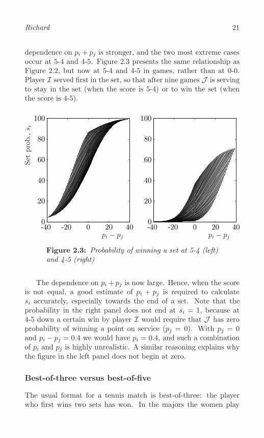
dependence on pi + pj is stronger, and the two most extreme casesoccur at 5-4 and 4-5. Figure 2.3 presents the same relationship asFigure 2.2, but now at 5-4 and 4-5 in games, rather than at 0-0.Player I served first in the set, so that after nine games J is servingto stay in the set (when the score is 5-4) or to win the set (whenthe score is 4-5).
Set
prob.,s i
-40 -20 0 20 40 0
20
40
60
80
100
pi − pj-40 -20 0 20 40
0
20
40
60
80
100
pi − pj
Figure 2.3: Probability of winning a set at 5-4 (left)and 4-5 (right)
The dependence on pi + pj is now large. Hence, when the scoreis not equal, a good estimate of pi + pj is required to calculatesi accurately, especially towards the end of a set. Note that theprobability in the right panel does not end at si = 1, because at4-5 down a certain win by player I would require that J has zeroprobability of winning a point on service (pj = 0). With pj = 0and pi − pj = 0.4 we would have pi = 0.4, and such a combinationof pi and pj is highly unrealistic. A similar reasoning explains whythe figure in the left panel does not begin at zero.
Best-of-three versus best-of-five
The usual format for a tennis match is best-of-three: the playerwho first wins two sets has won. In the majors the women play

22 Analyzing Wimbledon
best-of-three, but the men play best-of-five. In Figure 2.4 we plotthe probability mi that I wins the match as a function of pi − pj,for a cluster of values of pi + pj , calculated at the beginning ofthe match. Again we see that the dependence on pi − pj is muchstronger than the dependence on pi + pj .
Match
prob.,m
i
-40 -20 0 20 40 0
20
40
60
80
100
pi − pj
Figure 2.4: Probability of winning the match, best-of-five (dark) versus best-of-three (light)
The best-of-five curve (for the men) is always above the best-of-three curve (for the women) when pi > pj (and below whenpi < pj). This means that if I is a better player than J , then, fora given quality difference pi−pj > 0, the better player has a higherprobability of winning in a five-set match than in a three-set match.This makes sense, because the more points have to be played, thehigher is the probability that quality will show in the end. It isanother example of the magnification effect, introduced on page 16.For example, suppose that I and J are of equal strength (pi = pj)and that I can raise his or her game so that pi − pj is now 0.01.Then the match-winning probability mi will increase from 0.50 toabout 0.55 in a best-of-three match and to about 0.56 in a best-of-five match. We would therefore expect fewer ‘upsets’ in the men’ssingles than in the women’s singles at grand slam events. But isthis what happens?

Richard 23
Upsets
To answer this question we need to define what we mean by an‘upset’. At tennis tournaments a number of players are ‘seeded’ toavoid having to play against each other in the early rounds. A totalof 128 players feature in each grand slam singles event. For manyyears only the top-sixteen players were seeded. These seedings weresometimes subjective, because seedings were given to players whoperformed well on the particular surface of that tournament. Asa result, some players in the top sixteen would not get a seedingor would be seeded lower than their world ranking, while otherswho were not in the top sixteen would be seeded. Naturally thisannoyed some of the top players. The 2001 Wimbledon champi-onships paved the way for a new and more popular style of seeding,where the top-ranked thirty-two players are seeded for each grandslam tournament, irrespective of their history on a particular sur-face. This automatic seeding is now standard at all grand slamtournaments except Wimbledon, which still reserves the right todeviate from the official rankings. For the men’s singles, this devi-ation is determined by a formula: ATP points + grass court pointsduring the last twelve months + 75% of points earned from the bestgrass court tournament during the twelve months before that. Butfor the women’s singles there is no formula, just a recommendationto follow the WTA rankings ‘except where, in the opinion of thecommittee, a change is necessary to produce a balanced draw’.
Intuitively, an upset occurs when an unseeded player beats aseeded player. This is one possible definition of an upset, if wetake into account that sixteen players were seeded before 2001, butthirty-two from 2001 onwards. It is easier, however, and equallyintuitive to say that an upset has occurred when a top-sixteen playerdoes not reach the last sixteen, and this will be our definition of an‘upset’.
Of the four grand slams, most upsets occur at Wimbledon, bothfor the men and for the women. Indeed, in 2002 Lleyton Hewitt(seeded 1 and the champion that year) and Tim Henman (seeded 4)were the only top-sixteen seeds to reach the last sixteen.
On average, during the ninety-two grand slam events in theperiod 1990–2012 (twenty-three years, four events per year), 53%of the top-sixteen men and 62% of the top-sixteen women reached

24 Analyzing Wimbledon
the last sixteen. So there are more rather than fewer upsets forthe men than for the women, contrary to what the previous sectionpredicted. The only possible explanation is that the variation instrength pi − pj is much smaller for the men than for the women,and this corresponds to casual observation.
1990 2000 2010 0
20
40
60
80
100
1990 2000 2010 0
20
40
60
80
100
Figure 2.5: Percentage of top-sixteen seeds reachinglast sixteen, 1990–2012 (men left, women right)
Have the men always experienced more upsets? Figure 2.5 plotsthe development of the percentages over time. We see an increase(fewer upsets) for the men and a decrease (more upsets) for thewomen in the last few years. If we consider only the years 2009–2012 and average over these four years and the four grand slams,then 64% of the top-sixteen men and 54% of the top-sixteen womenreached the last sixteen. This comes closer to what we would expectbased on the difference between best-of-three and best-of-five, andthus shows indirectly that the variation in strength has becomelarger for the men or smaller for the women or both. We return tothis issue in Chapter 7 when we discuss hypothesis 12.
Long matches: Isner-Mahut 2010
Long matches occur from time to time. The 1969 first-round Wim-bledon match between Pancho Gonzales and Charlie Pasarell lasted112 games, but this was before the introduction of the tiebreak. Atthe US Open tiebreaks are played in all sets, including the final set,but in the other three grand slam tournaments there is no tiebreakin the final set and hence long final sets can occur. Andy Roddick

Richard 25
defeated Younes El Aynaoui at the 2003 Australian Open quar-ter final in a five-set thriller with a score of 21-19 in the final set(eighty-three games in total), but this was nothing compared to theextraordinary match in which John Isner defeated Nicolas Mahutin the first round of Wimbledon 2010 after eleven hours and fiveminutes (over three days), with a score of 6-4, 3-6, 6-7, 7-6, 70-68(183 games, 980 points).
At the grand slams almost 20% of the men’s matches go to fivesets. At the three grand slams where a tiebreak is not played inthe final set, the number of ‘long’ (lasting at least fourteen games)fifth sets is about 15%. Since there are 127 matches to be playedin each tournament, we would expect 0.20 × 0.15 × 127 (that is,about four) long matches every year in each of the Australian Open,Roland Garros, and Wimbledon. Interestingly, there are also (onaverage) about four long matches in each women’s tournament.This is because there are more final (third) sets, about 30%, butfewer of these are long, about 10%.
For a statistician to investigate an extreme event such as theIsner-Mahut match, the difficulty lies in the fact that very few ob-servations are available. Very long matches are very rare. In sucha situation we need more theory and more structure to producecredible results. Below we provide a mathematical analysis with aminimum of empirical observations. Still, the analysis allows us tomake statements about how special the Isner-Mahut match was.
In calculating the probability of a long match we shall assumethat hypothesis 1 holds, so that the points are iid. In addition, weshall assume that both players I and J have the same probabilitypi = pj of winning their service point. Hence, they are equallystrong. This is the situation where long matches can occur andhence the case of interest to us. Under these two assumptions, bothplayers have the same probability, denoted by g, to win a servicegame.
Next we observe that for a long match to occur two ‘knots’ mustbe passed. The players must reach 2-2 in sets and in the final setthey must reach 5-5 in games. There is no other way that a longmatch can develop. As a result, we can do the calculations in threesteps.
First, the probability of reaching 2-2 in sets equals 3/8. This isbecause we have assumed that pi = pj, so that the probability that

26 Analyzing Wimbledon
I wins a set is 1/2. There are six possibilities to reach 2-2 in sets:
IIJJ , IJIJ , IJJ I, JIIJ , J IJI, JJ II.
Each of these has a probability of 1/16. Hence the probabilityof reaching 2-2 in sets is 6/16 = 3/8. This is an example of thebinomial probability distribution.
Second, we can use the binomial distribution to obtain the prob-ability of reaching the score 5-5 in a set when both players haveprobability g to win their service game. This is more difficult andwe simply denote this probability by �(5, 5) (� for likelihood). Thehigher g, the more likely 5-5 becomes.
Third, we compute the probability that — given a 5-5 score inthe final set — the set is decided with a score of a-b (a games for Iand b games for J ). Multiplying this probability with �(5, 5) gives�(a, b), the probability that the final set reaches the score a-b. Theprobability that two players of equal strength have to compete untila-b in the final set is then equal to (3/8) × �(a, b). Obviously, b-ahas the same probability.
What is the probability of a match as extreme as the Isner-Mahut match, that is, a match ending 70-68 in the final set? Itis
2× (3/8) × �(70, 68).
More important is the probability of a match at least as extremeas the Isner-Mahut match. This probability is given by
2× (3/8) × (�(70, 68) + �(71, 69) + �(72, 70) + . . .
),
which depends only on the game-winning probability g which, inturn, depends only on the common point probability p. Table 2.2presents the implied probabilities for each of four values of p.
Point prob., p 60 70 80 90
Game prob., g 73.6 90.1 97.8 99.9Prob. of long match 3.6×10⁻¹³ 7.1×10⁻⁵ 2.0 30.8
Table 2.2: Probability (in %) of a match as long asor longer than Isner-Mahut

Richard 27
On average, the probability of winning a point of service is about67% at Wimbledon (for the men; for the women it is 59%). Atthe Isner-Mahut match John Isner won 76.2% of the points on hisservice and Nicolas Mahut 78.7%. Hence the assumption pi = pjis not unreasonable. The probability of two players of about equalstrength with such high values of p playing against each other issmall. But if they meet, then the probability of a long match is notthat small: for p = 80% the probability of a match with a fifth setas long or longer than Isner-Mahut is 2%.
Rule changes: the no-ad rule
Rule changes are regularly discussed in order to make matches moreexciting and attractive to watch. Rules to make matches shorterinclude the tiebreak (now standard), but also more controversialproposals such as the ‘match tiebreak’, the ‘short set’, and the ‘no-ad’ rule. These alternatives have long been used by amateurs andin selected competitions, such as World Team Tennis and Intercol-legiate Tennis, but they were only formally recognized in the ITFRules of Tennis from 2002 onwards.
A match tiebreak (also called supertiebreak) replaces the final set.Instead of playing a final set, one plays an extra long tiebreak:a match tiebreak. The winner of a match tiebreak is theplayer who reaches ten points first (rather than seven as inthe ordinary tiebreak) with at least a two-point advantage. Ifa two-point advantage is not reached then the match tiebreakcontinues until it is.
A short set is a four-game set where the first to win at least fourgames with a margin of at least two games wins the set. Atiebreak is played at four-games-all. This rule is sometimesproposed together with playing best-of-five sets in all tourna-ments for both men and women.
The no-ad rule replaces the deuce system. The first player to winfour points wins the game, even if the score is deuce. At deuceonly one more point is played and the receiver has the choiceof deuce court (right) or ad court (left).

28 Analyzing Wimbledon
The match tiebreak and the no-ad rule are currently being used fordoubles matches in ATP and WTA tournaments, but not in thegrand slam tournaments. These rules lead to shorter and more pre-dictable (in terms of time) doubles matches — in statistical terms,they lead to a lower mean and a lower variance in match length.Although the doubles players were initially opposed, they were per-suaded with the promise of more doubles matches on the principalcourts. It was also hoped that more of the top singles players wouldplay doubles with this format.
An experiment to play best-of-five sets for both men and womenbut with ‘short sets’ was conducted in the late 1990s at lower ITFtournaments, but the players’ response was negative and the trialdiscontinued.
Let us consider the no-ad rule. If the traditional scoring systemat deuce would be replaced by the no-ad rule, so that only onedeciding point is played at deuce, then the probability gi on page 15that I wins the game would change to
gi = p4i (−20p3i + 70p2i − 84pi + 35).
It is easy to see that for pi > 0.5 (the most common case), wehave gi < gi, so that more service breaks will occur. The largestdiscrepancy occurs at pi = 0.65, where gi = 0.83 and gi = 0.80, andthe probability of a break thus increases from 17% to 20%.
Abolishing the second service
Rules have also been proposed to reduce the service dominance.One could allow larger balls, which would imply better visibility ontelevision and slower movement through the air. Such balls have infact been produced, but they are seldom used. The most obviousrule change, however, would be to abolish the second service. Thereis no particular reason why the server should have two possibilitiesto serve and there is no other sport where such a rule exists. BillTilden, a ten-time grand slam winner, speculated in 1920 that thesecond service would eventually be abolished, but so far he has beenproven wrong. What would be the consequence of abolishing thetwo-service rule?
Most people — when asked this question — respond that withonly one service a player would serve ‘somewhere in-between’ his or

Richard 29
her current first and second service. But this would not be a goodstrategy. The correct strategy is to simply forget about the currentfirst service and always use the current second service. It is easyto see why. A player with only one service is equivalent to a playerwith two services having faulted the first service. So, with only oneservice, a player should use his or her current second service, notsomething in-between. In the language of game theory (a branchof mathematics), the current situation (with two services) has asubgame (the second service) and in a subgame perfect equilibriumone plays the second service as in the equilibrium of the game inwhich only one service is available. Hence, the proposed change toone service actually amounts to abolishing the first service.
To see the effect of this proposal we consider the probability ofwinning a point on service. Under the current two-service rule thisprobability is quantified by the relative frequencies in Table 2.1.Data under the proposed one-service rule are not available, be-cause this rule is currently not applied. However, the above game-theoretical argument implies that we can simply take the relativefrequency of winning a point on the second service, and these dataare available.
Men Women2 serves 1 serve 2 serves 1 serve
Australian Open 62.2 49.9 55.4 44.8Roland Garros 62.4 50.6 55.7 44.9Wimbledon 66.7 51.9 59.3 46.9US Open 63.6 51.4 55.7 44.8
Table 2.3: Estimated probability of winning a pointon service under the two- and one-service rules, re-spectively, 2010 data
Table 2.3 shows that at Wimbledon the probability of winning apoint on service for the men would decrease from 66.7% to 51.9%,still a service advantage, but much smaller than before. For thewomen, it would decrease from 59.3% to 46.9%. Here the serviceadvantage would turn into a disadvantage. The idea of a servicedisadvantage may seem strange to tennis fans. But there are many

30 Analyzing Wimbledon
sports (such as volleyball) where this is the case. Both new per-centages are closer to 50% than before. Hence there will be morebreaks and the probability of very long matches will be reduced.
One might argue that, if the one-service rule is implemented,players will spend more time practicing that service, so that thewinning probability may increase. On the other hand, players willalso adjust their training on returning the single service, thus re-ducing the service-winning probability. The overall training effectcan go either way, and we ignore it.
Other consequences of rule changes, particularly on the optimalservice strategy, will be examined in Chapter 9.
Further reading
The assumption that points are iid has been the subject of severalstudies. Klaassen and Magnus (2001) show that iid is rejected butthat deviations from iid are small, particularly for top players, sothat imposing iid will still provide a good approximation in manycases (see also Chapter 10). Newton and Aslam (2006) confirmthe latter result, even when relatively strong non-iid effects areintroduced in their simulations. But is it optimal to play points ‘asthey come’ and play (close to) iid? Walker et al. (2011) derive thatit is indeed optimal to ignore the score, that is, play according toan identical distribution.
Under iid one can calculate the probability of winning a game,set, tiebreak, or match, as Richard does. This has a long history,beginning with Kemeny and Snell (1960, pp. 161–167), and includ-ing Hsi and Burych (1971), Morris (1977) (who also discusses themagnification effect), Riddle (1988, 1989) (who also proves thatserving first in a set does not matter under iid), and Newton andKeller (2005).
These approaches have been used to study the tennis scoringsystem and its effect on the probability of winning a match, natu-rally leading to some new proposals for rule changes. Pollard (1983)shows that the better player wins more often in a classical set (with-out tiebreak) than in a tiebreak set. Miles (1984) argues that intop men’s tennis the proportion of service points won is so highthat many points have to be played to identify the better player.It would be more efficient (and also lead to shorter matches, easier

Richard 31
for television scheduling) to begin each game at 0-30 rather than at0-0. Another innovative idea is due to Pollard and Noble (2004),who suggest the ‘50-40 game’: the server must still win four pointsin order to win the game (reach score 50), but the receiver requiresonly three points in order to win it (40). This leads to a more pre-dictable match duration in a match between strong servers. For ananalysis of the consequences of abolishing the second service, seeKlaassen and Magnus (2000).
Regarding upsets, Boulier and Stekler (1999) report that ingrand slam tournaments during 1985–1995, 53% of seeded maleplayers and 63% of seeded female players reached the last sixteen.The 1990–2012 results in this book (53% and 62%, respectively)are similar. Magnus and Klaassen (1999c) find that for the men aseeded player beats a non-seed somewhat less frequently than forthe women. All results suggest that men’s tennis is more competi-tive than women’s tennis. A more powerful analysis confirming thisstatement will be provided when we test hypothesis 12 in Chapter 7.

This page intentionally left blank

3Forecasting
The use of statistics has become increasingly popular in sports.Television broadcasts inform us about the percentage of ball pos-session in football, the number of home runs in baseball, and thenumber of aces and double faults in tennis. All these statistics pro-vide some insight into the question which player or team performsparticularly well in a match, and therefore also (indirectly) into thequestion who is more likely to win. Surprisingly, however, a directestimate of the probability that a player or a team wins the matchis not shown.
In this chapter we provide such a direct estimate for tennis.We forecast the winner of a match, not only at the beginning ofthe match, but also while the match is unfolding; in fact, at eachpoint. The forecast is produced within one second after each point,and the resulting profile of winning probabilities provides a quickoverview of the match developments so far and a direct forecast ofwho will win the match. The quality of the profile is confirmed bythe probabilities implied by in-play betting odds.
The profile provides valuable insights for fans and commentatorswatching a tennis match. The score itself, obviously an importantingredient in forecasting the outcome, tells us which player is lead-ing, but this does not imply that this player is also likely to winthe match: a top player may still be the favorite after losing thefirst set. Moreover, a score of 5-5 can result after 4-4, but also after5-0, so that the score provides only partial information on the de-velopment of the match so far. Summary statistics do not fill thesevoids, but a graph of winning probabilities does. The profile shouldthus prove to be a powerful tool for commentators and viewers.
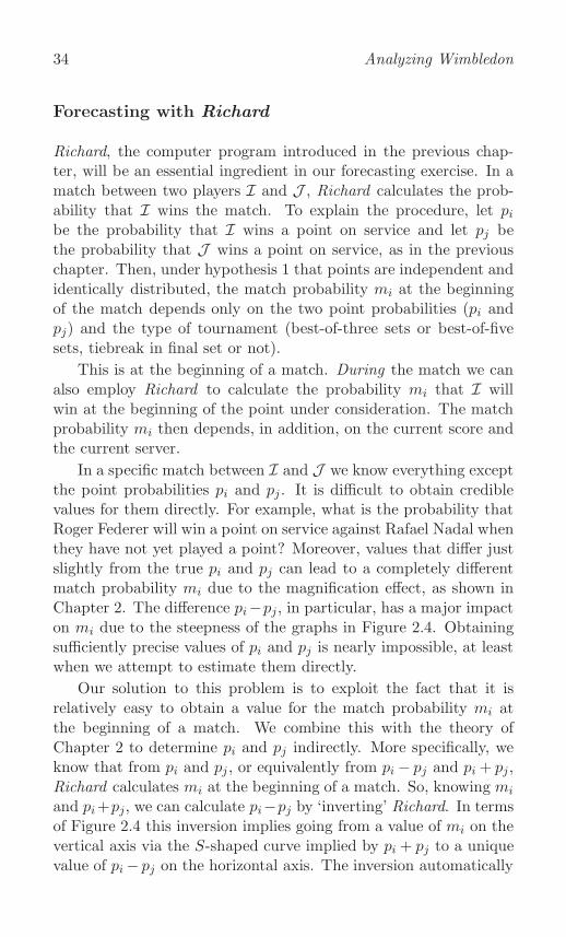
34 Analyzing Wimbledon
Forecasting with Richard
Richard, the computer program introduced in the previous chap-ter, will be an essential ingredient in our forecasting exercise. In amatch between two players I and J , Richard calculates the prob-ability that I wins the match. To explain the procedure, let pibe the probability that I wins a point on service and let pj bethe probability that J wins a point on service, as in the previouschapter. Then, under hypothesis 1 that points are independent andidentically distributed, the match probability mi at the beginningof the match depends only on the two point probabilities (pi andpj) and the type of tournament (best-of-three sets or best-of-fivesets, tiebreak in final set or not).
This is at the beginning of a match. During the match we canalso employ Richard to calculate the probability mi that I willwin at the beginning of the point under consideration. The matchprobability mi then depends, in addition, on the current score andthe current server.
In a specific match between I and J we know everything exceptthe point probabilities pi and pj . It is difficult to obtain crediblevalues for them directly. For example, what is the probability thatRoger Federer will win a point on service against Rafael Nadal whenthey have not yet played a point? Moreover, values that differ justslightly from the true pi and pj can lead to a completely differentmatch probability mi due to the magnification effect, as shown inChapter 2. The difference pi−pj, in particular, has a major impacton mi due to the steepness of the graphs in Figure 2.4. Obtainingsufficiently precise values of pi and pj is nearly impossible, at leastwhen we attempt to estimate them directly.
Our solution to this problem is to exploit the fact that it isrelatively easy to obtain a value for the match probability mi atthe beginning of a match. We combine this with the theory ofChapter 2 to determine pi and pj indirectly. More specifically, weknow that from pi and pj , or equivalently from pi − pj and pi + pj,Richard calculates mi at the beginning of a match. So, knowing mi
and pi+pj, we can calculate pi−pj by ‘inverting’ Richard. In termsof Figure 2.4 this inversion implies going from a value of mi on thevertical axis via the S-shaped curve implied by pi + pj to a uniquevalue of pi− pj on the horizontal axis. The inversion automatically

Forecasting 35
circumvents the problem that small deviations in pi − pj have amajor impact on mi, because we start from mi, not from pi − pj .We thus transform the initial problem of finding pi and pj into two(easier) problems: finding mi at the beginning of the match andfinding pi + pj. From mi and pi + pj we first derive pi − pj, andthen pi and pj themselves. How do we know mi at the beginningof a match and how do we determine pi + pj?
There are several ways to estimate mi at the beginning of amatch. One could use the rankings of the two players. This worksreasonably well in practice but it has the disadvantage that thecourt surface (grass, clay) is not taken into account and also thatrecent information such as a minor injury is ignored.
A different way, incorporating all publicly available information,is to use betting odds. The fractional odds in favor of an event aredefined as the ratio of the probability that the event will happen tothe probability that it will not happen. For example, the fractionalodds that a randomly chosen day of the week is a Sunday are oneto six, written as 1:6. This system is favored in the United King-dom and Ireland and is common in horse racing, but it is a littlecounterintuitive.
More intuitive are the decimal odds, which are simply the in-verse probability. The decimal odds that a randomly chosen day ofthe week is a Sunday are seven to one, written as 7.0. If the decimalodds of I defeating J are 1.5, then mi is the inverse, so mi = 2/3.In fact, the transformation from betting odds to match probabil-ity mi is a little more complex, because the decimal odds do notrepresent the true inverse probabilities as perceived by the book-maker, but are the amounts that the bookmaker will pay out onwinning bets. In formulating his odds the bookmaker will includea profit margin, the so-called overround on his book, for which wewill account when computing mi.
We also need a value for pi + pj. This too can be achieved inseveral ways. Using the rankings of the two players and a statisticalmodel is one option. But a simpler alternative is to just set pi +pj = 2p, where p denotes the tournament average of the players’point-winning probability p in a representative year. This averagecan easily be estimated by combining the summary statistics ofall matches in that year, and Table 2.1 presents the values for thegrand slam tournaments in 2010. We shall use this simpler method

36 Analyzing Wimbledon
in the analysis below.
The reason that the simple method works in practice is that, atmany points, mi does not much depend on pi+pj, as we saw in theprevious chapter. Still, there may be points where pi + pj matters.For two players I and J in a specific match, we should performa sensitivity analysis to check whether the match profile changeswhen the estimate of pi + pj is changed. We shall do so below andconclude that the influence on the match profile is small and thatthe proposed simple method thus accurately estimates the matchprobabilities.
Summarizing, we calculate the probability mi that I will winthe match against J as follows. First we compute mi at the begin-ning of the match from betting odds. Then we compute p as thetournament average in a comparable year, and set pi + pj = 2p.Given mi and pi + pj we then call on Richard to produce pi − pj.Once we have pi + pj and pi − pj, we also have pi and pj sepa-rately, so that we can compute mi, not only at the beginning of thematch, but at each point as the match unfolds. Richard calculatesvery quickly, and the updated mi is available within a second aftercompletion of the point.
Federer-Nadal, Wimbledon final 2008
We illustrate the forecasting procedure by analyzing three famousmatches. First, the 2008 Wimbledon final between Roger Federer(seeded 1) and Rafael Nadal (seeded 2). Federer had won the fiveprevious finals at Wimbledon and had he won this time he wouldhave become the first man since William Renshaw (1881–1886) towin a sixth consecutive championship at The All England LawnTennis and Croquet Club. He came close, but in the end he lost4-6, 4-6, 7-6, 7-6, 7-9 in arguably the best match ever played atWimbledon. It was Nadal’s first Wimbledon title, having lost toFederer in the 2006 final in four sets, and in the 2007 final in five.
At the beginning of the match Federer was the favorite. Letus call him player I and Nadal player J . Averaging over fivebetting sites, we obtain decimal betting odds of bi = 1.691 (Fed-erer) and bj = 2.198 (Nadal). Direct calculation of the match-winning probabilities would give 1/bi = 0.591 and 1/bj = 0.455,respectively. These two ‘probabilities’ add up to 1.046, hence more

Forecasting 37Prob.Fed
erer
wins
50 100 150 200 250 300 350 400 0
20
40
60
80
100set 1 set 2 set 3 set 4 set 5
Point number
Figure 3.1: Federer-Nadal profile, Wimbledon 2008(p = 66.7%)
than one because of the overround. Correcting for this we obtainmi = 0.591/1.046 = 0.565 and mj = 0.455/1.046 = 0.435. Hencewe estimate the initial probability that Federer wins as mi = 56.5%.
From Table 2.1 we find p = 66.7%. From pi + pj = 2p = 1.334and mi = 0.565 we call on (inverted) Richard to calculate pi −pj = 0.011. This then gives pi = 67.2% (Federer) and pj = 66.2%(Nadal) from which the match profile can be computed.
The match profile is presented in Figure 3.1 from Federer’s pointof view. At the beginning of the match Federer’s probability ofwinning was 56.5%. After losing the first two sets, this probabilityhad dropped to 15.3%, but when Federer won the third-set tiebreakhis probability of winning the match went up again, to 28.7%. Bigswings occurred at the end of the fourth set. Nadal led 5-2 in thetiebreak, then double-faulted to 5-3. At 7-6 and again at 8-7, Nadalhad matchpoints (the second time on his own service). EventuallyFederer won the tiebreak 10-8.
No man had come back to win a Wimbledon final after losingthe first two sets since Henri Cochet defeated Jean Borotra in 1927,

38 Analyzing Wimbledon
but at 2-2 in sets Federer was still favorite to win with probability53.8%, smaller than the original 56.5% (because of the magnifica-tion effect) but larger than 50%. In the final set, Federer was 4-3ahead and had breakpoint on Nadal’s service. His probability ofwinning the match was then 72.9%, the highest of the match. ButNadal held serve. Two games later, at 5-4, Federer needed onlytwo points for the championship and his probability of winning was62.9%. Again Nadal held service. At 5-5 Federer was two break-points down. Commentators were quick to point out that Federer’sdisappointment of missing the earlier chances had affected the mo-mentum in Nadal’s favor. Whether the commentators were rightor wrong will be considered in Chapter 12, where we ask the gen-eral question of whether missed breakpoint(s) in one game lead toa larger probability of being broken in the next (hypothesis 22).Federer’s probability dropped to 27.1%, but he managed to savethe breakpoints. Both players continued to hold service until 7-7.Then Federer lost his service and Nadal served for the match towin 9-7 in the final set. After the last point the probability thatFederer wins is obviously zero.
The profile provides a graphical illustration of the changing for-tunes during the match, not only qualitatively but also quantita-tively. A comparison with the 50% line makes it immediately clearwho the current favorite is, and also by how much. Moreover, thegraph can be produced while the match is in progress — we don’thave to wait until the match is completed.
Effect of smaller p
We already mentioned a possibly weak link in the theory underlyingthe graph, namely the determination of pi + pj . In computing theprofile we used the tournament average p in a representative year,and set pi + pj = 2p. This is simple, perhaps too simple. What isthe effect when we refine the estimate of pi + pj?
At the 2006 Wimbledon final between Roger Federer and RafaelNadal they realized pi+pj = 1.320, and at the 2007 final 1.339. (Atthe 2008 Wimbledon final between Federer and Nadal they realizedpi + pj = 1.337, but of course we only knew this at the end of thematch, so we could not use it during the match.) This correspondsto taking p = 66.0% in 2006, 66.9% in 2007, and 66.8% in 2008.
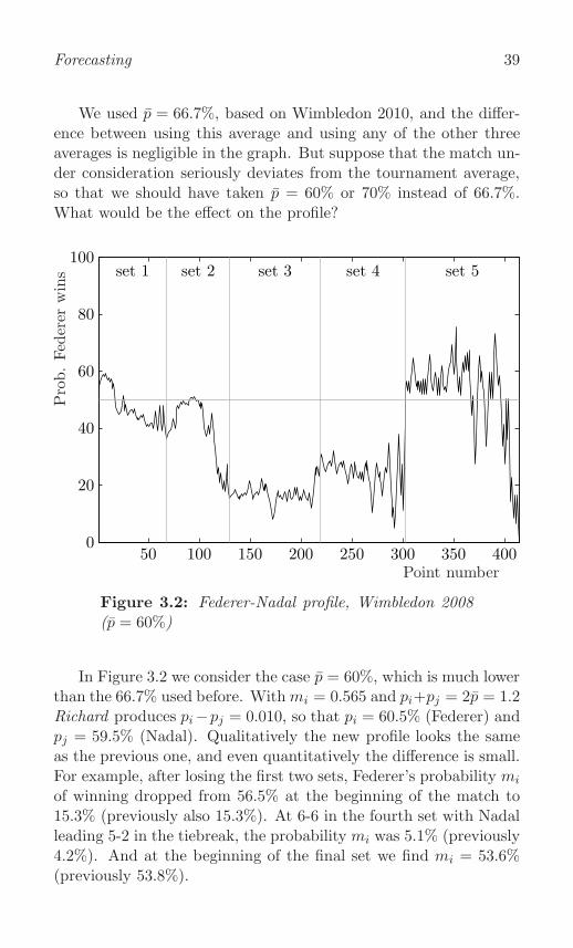
Forecasting 39
We used p = 66.7%, based on Wimbledon 2010, and the differ-ence between using this average and using any of the other threeaverages is negligible in the graph. But suppose that the match un-der consideration seriously deviates from the tournament average,so that we should have taken p = 60% or 70% instead of 66.7%.What would be the effect on the profile?
Prob.Fed
erer
wins
50 100 150 200 250 300 350 400 0
20
40
60
80
100set 1 set 2 set 3 set 4 set 5
Point number
Figure 3.2: Federer-Nadal profile, Wimbledon 2008(p = 60%)
In Figure 3.2 we consider the case p = 60%, which is much lowerthan the 66.7% used before. Withmi = 0.565 and pi+pj = 2p = 1.2Richard produces pi−pj = 0.010, so that pi = 60.5% (Federer) andpj = 59.5% (Nadal). Qualitatively the new profile looks the sameas the previous one, and even quantitatively the difference is small.For example, after losing the first two sets, Federer’s probability mi
of winning dropped from 56.5% at the beginning of the match to15.3% (previously also 15.3%). At 6-6 in the fourth set with Nadalleading 5-2 in the tiebreak, the probability mi was 5.1% (previously4.2%). And at the beginning of the final set we find mi = 53.6%(previously 53.8%).

40 Analyzing Wimbledon
These numbers confirm what we found in Chapter 2. The profileis not sensitive to the specification of pi + pj.
Kim Clijsters defeats Venus Williams, US Open 2010
Venus Williams (seven grand slam singles titles) won both Wimble-don and the US Open in 2000 and 2001, and she won Wimbledonagain in 2005, 2007, and 2008. Kim Clijsters won the US Openin 2005. The next three years she did not participate, but in 2009she received a wildcard and, only one month after her return to theprofessional tour, she won again, defeating Caroline Wozniacki inthe final. In 2010, Clijsters (seeded 2) met Williams (seeded 3) inthe semi-final, and defeated her in a memorable three-set match:4-6, 7-6, 6-4.
Prob.Clijsters
wins
20 40 60 80 100 120 140 160 180 0
20
40
60
80
100
set 1 set 2 set 3
Point number
Figure 3.3: Clijsters-Williams profile, US Open 2010(p = 55.7%)
Clijsters, the defending champion, was the favorite at the be-ginning of the match. Averaging over five betting sites, we finddecimal odds of bi = 1.452 (Clijsters) and bj = 2.732 (Williams).
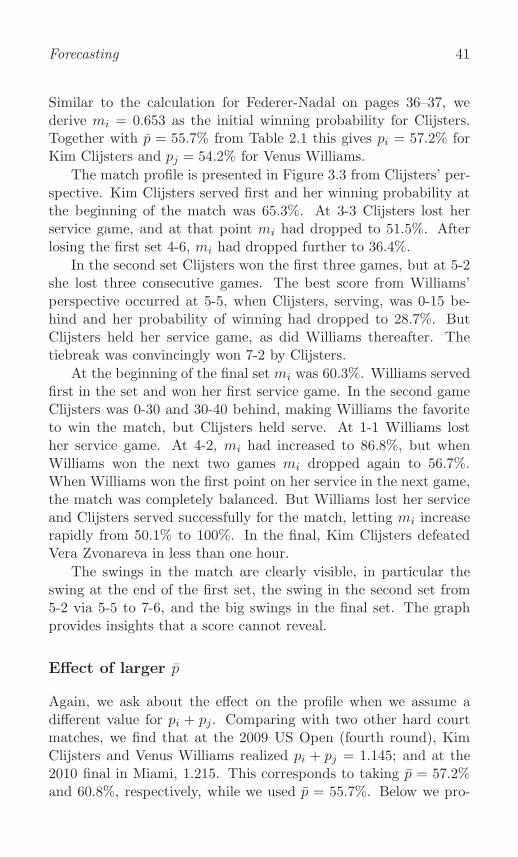
Forecasting 41
Similar to the calculation for Federer-Nadal on pages 36–37, wederive mi = 0.653 as the initial winning probability for Clijsters.Together with p = 55.7% from Table 2.1 this gives pi = 57.2% forKim Clijsters and pj = 54.2% for Venus Williams.
The match profile is presented in Figure 3.3 from Clijsters’ per-spective. Kim Clijsters served first and her winning probability atthe beginning of the match was 65.3%. At 3-3 Clijsters lost herservice game, and at that point mi had dropped to 51.5%. Afterlosing the first set 4-6, mi had dropped further to 36.4%.
In the second set Clijsters won the first three games, but at 5-2she lost three consecutive games. The best score from Williams’perspective occurred at 5-5, when Clijsters, serving, was 0-15 be-hind and her probability of winning had dropped to 28.7%. ButClijsters held her service game, as did Williams thereafter. Thetiebreak was convincingly won 7-2 by Clijsters.
At the beginning of the final set mi was 60.3%. Williams servedfirst in the set and won her first service game. In the second gameClijsters was 0-30 and 30-40 behind, making Williams the favoriteto win the match, but Clijsters held serve. At 1-1 Williams losther service game. At 4-2, mi had increased to 86.8%, but whenWilliams won the next two games mi dropped again to 56.7%.When Williams won the first point on her service in the next game,the match was completely balanced. But Williams lost her serviceand Clijsters served successfully for the match, letting mi increaserapidly from 50.1% to 100%. In the final, Kim Clijsters defeatedVera Zvonareva in less than one hour.
The swings in the match are clearly visible, in particular theswing at the end of the first set, the swing in the second set from5-2 via 5-5 to 7-6, and the big swings in the final set. The graphprovides insights that a score cannot reveal.
Effect of larger p
Again, we ask about the effect on the profile when we assume adifferent value for pi + pj. Comparing with two other hard courtmatches, we find that at the 2009 US Open (fourth round), KimClijsters and Venus Williams realized pi + pj = 1.145; and at the2010 final in Miami, 1.215. This corresponds to taking p = 57.2%and 60.8%, respectively, while we used p = 55.7%. Below we pro-
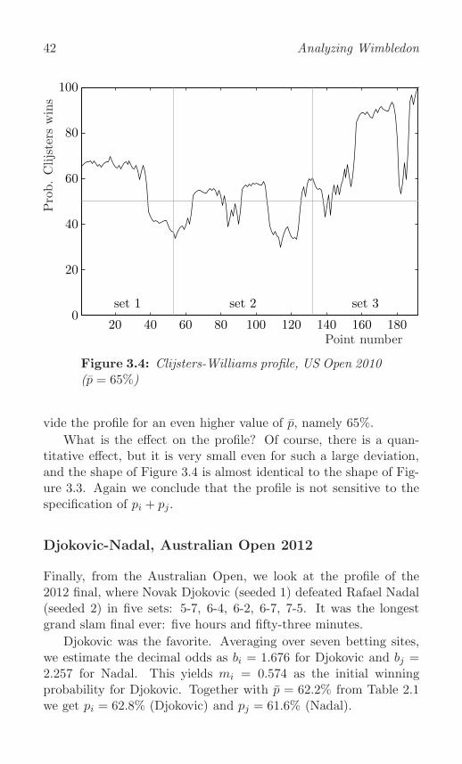
42 Analyzing WimbledonProb.Clijsters
wins
20 40 60 80 100 120 140 160 180 0
20
40
60
80
100
set 1 set 2 set 3
Point number
Figure 3.4: Clijsters-Williams profile, US Open 2010(p = 65%)
vide the profile for an even higher value of p, namely 65%.
What is the effect on the profile? Of course, there is a quan-titative effect, but it is very small even for such a large deviation,and the shape of Figure 3.4 is almost identical to the shape of Fig-ure 3.3. Again we conclude that the profile is not sensitive to thespecification of pi + pj.
Djokovic-Nadal, Australian Open 2012
Finally, from the Australian Open, we look at the profile of the2012 final, where Novak Djokovic (seeded 1) defeated Rafael Nadal(seeded 2) in five sets: 5-7, 6-4, 6-2, 6-7, 7-5. It was the longestgrand slam final ever: five hours and fifty-three minutes.
Djokovic was the favorite. Averaging over seven betting sites,we estimate the decimal odds as bi = 1.676 for Djokovic and bj =2.257 for Nadal. This yields mi = 0.574 as the initial winningprobability for Djokovic. Together with p = 62.2% from Table 2.1we get pi = 62.8% (Djokovic) and pj = 61.6% (Nadal).
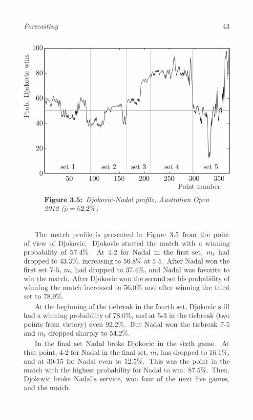
Forecasting 43Prob.Djokovic
wins
50 100 150 200 250 300 350 0
20
40
60
80
100
set 1 set 2 set 3 set 4 set 5
Point number
Figure 3.5: Djokovic-Nadal profile, Australian Open2012 (p = 62.2%)
The match profile is presented in Figure 3.5 from the pointof view of Djokovic. Djokovic started the match with a winningprobability of 57.4%. At 4-2 for Nadal in the first set, mi haddropped to 43.3%, increasing to 56.8% at 5-5. After Nadal won thefirst set 7-5, mi had dropped to 37.4%, and Nadal was favorite towin the match. After Djokovic won the second set his probability ofwinning the match increased to 56.0% and after winning the thirdset to 78.9%.
At the beginning of the tiebreak in the fourth set, Djokovic stillhad a winning probability of 78.0%, and at 5-3 in the tiebreak (twopoints from victory) even 92.2%. But Nadal won the tiebreak 7-5and mi dropped sharply to 54.2%.
In the final set Nadal broke Djokovic in the sixth game. Atthat point, 4-2 for Nadal in the final set, mi has dropped to 16.1%,and at 30-15 for Nadal even to 12.5%. This was the point in thematch with the highest probability for Nadal to win: 87.5%. Then,Djokovic broke Nadal’s service, won four of the next five games,and the match.

44 Analyzing Wimbledon
In-play betting
Our forecasting profiles are based on Richard, a computer program,which in turn is based on a model. The only assumption in thismodel is that the service points of each player in a match are iid.The three match examples suggest that the profiles provide a re-alistic picture of the matches involved, and hence provide indirectevidence that the model makes sense. But what does ‘the market’tell us about the quality of our profiles?
The emergence of in-play tennis betting markets allows us tocompare our Richard-based forecasts to the forecasts implied bybetting odds. We focus on one match, the Federer-Nadal Wimble-don 2008 final. To compare the market forecasts to our profiles weneed a market assessment of the probability that Federer wins thematch at each point of the match.
The market’s view is computed from realized trades at Betfair,an online betting company launched in 2000. Betfair is an exchangewhere one gambler bets against another gambler (hence not againsta bookmaker). Betfair acts as an intermediary and earns commis-sion on the profit of a winning gambler. This implies that there isno profit margin in the odds themselves (overround) as in the caseof a bookmaker.
From the matched odds one can directly infer the implied prob-ability of an event. More specifically, the probability that Federerwins the match is the inverse of the (decimal) odds on Federer towin. An important match such as a Wimbledon final attracts alarge amount of betting. The value of matched bets was six mil-lion pounds at the beginning of the match, and increased to fiftymillion pounds at the end. The market is therefore big enoughto consider the implied probabilities as the market’s view on theevolving probabilities that Federer wins the match.
From a few hours before the match until the end of the matchthe probability is available, not point by point but second by sec-ond. Our model-based probability is measured at each point, notat each second. In order to provide a comparison we transformedthe Betfair data to our format, thus obtaining the market’s winningprobability at the beginning of each point.
Figure 3.6 replicates our forecast profile from Figure 3.1 (darkline) and adds the Betfair probabilities (light line). The correspon-

Forecasting 45Prob.Fed
erer
wins
50 100 150 200 250 300 350 400 0
20
40
60
80
100set 1 set 2 set 3 set 4 set 5
Point number
Figure 3.6: Model (dark) and Betfair (light) profiles,Federer-Nadal at Wimbledon 2008
dence is striking, in fact so striking that the only credible explana-tion is that Betfair traders and their computers are using our modelor a model very similar to ours.
Let us take a closer view. At the beginning of the match the twoprobabilities virtually coincide, with our approach giving Federer56.5% chance to win and Betfair 57.5%. This is not surprising,because our starting probability is derived from the bookmakersodds. As the match unfolds, some differences between the twographs emerge, not so much in the movement from one point tothe next, but rather in the level. From the middle of the first setuntil halfway through the fourth the Richard probabilities are about10%-points below the Betfair probabilities. For example, at 0-1 insets, 4-2 in games, and 30-30 in points on Federer’s service (point103), the probabilities are 50.6% and 58.1%, respectively. This is alarge difference. In fact too large, given the starting probability ofaround 57%. It is difficult to explain why Federer’s match-winningprobability at this point would be higher than at the beginning ofthe match. Still, this is apparently what the market believed.

46 Analyzing Wimbledon
How to explain this discrepancy? Let us use to same startingpoint as Betfair, that is, 57.5% rather than 56.5%. This increasesthe probability at point 103 from 50.6% to 51.5%, a slight increase,but insufficient to explain such a large discrepancy. Recall frompage 35 that, apart from the initial match probability, our methodrequires an estimate of the sum of the point-winning probabilitiespi and pj of Federer and Nadal. However, Figure 3.2 shows that,even if we decrease or increase this sum substantially, it does notmuch affect the probability at point 103.
The only remaining explanation is that Betfair traders allowfor deviations from the iid assumption. For example, they mightthink that the favorite will win more often than predicted under theiid assumption, if the favorite is behind. This raises an interestingquestion: can such deviations from iid be uncovered from the data?We shall come back to this question in Chapters 10–12, where wediscuss and apply methods to test for deviations from iid.
Further reading
In-play forecasting of the winner of a match dates back to Mag-nus and Klaassen (1995, 1997). There we used the seeding list toestimate the initial match-winning probability (the starting pointof the profile). Using betting odds, as implemented in this book,appears to be an improvement.
Several alternatives for estimating the initial probability exist,based on past performances of the players. Blackman and Casey(1980) use match scores, while Clarke and Dyte (2000) use world-ranking points. Klaassen and Magnus (2003a,b,c; 2008) employ thepositions on the world ranking, although the user of the profile (say,the commentator) can adjust the estimate to account for his or herown specific knowledge, such as special abilities of the players onthe court surface or health problems. McHale and Morton (2011)utilize games won and lost in past matches and the time passedsince these matches were played to capture recent form.
Barnett (2006) describes in-play forecasting and how it has beenused since Wimbledon 2003 for setting bookmaker prices for bet-ting on the point score in completed games, that is, the server orreceiver winning to 0, 15, 30, or deuce. Jackson (1994) predicteda booming sports-betting market, and the introduction of Betfair

Forecasting 47
has validated this prediction; see Davies et al. (2005) for detailson Betfair. The resulting forecasts are now also used for statisti-cal analysis outside the betting scene. For example, Easton andUylangco (2010) compare the predictions from our model to thosederived from Betfair odds for forty-nine matches at the 2007 Aus-tralian Open and conclude that there is a very high correlation,again implying that the model predictions make sense.

This page intentionally left blank

4Importance
Are all points equally important? Or are some points more impor-tant than others? If so, what are the ‘big’ points? Is 15-30 themost important point in a game? After all, if you (the server) winthe point, then the score is 30-30 and you will probably win thegame. But if you lose the point, it is 15-40 and you will probablylose the game. Is the seventh game the most important in a set, asone often hears? Which are the most important points in a match?All these questions relate to the concept of ‘importance’.
What is importance?
Intuitively, a point is important within a game if winning or losingthe point has a large impact on winning the game. Likewise, a gameis important within a set if winning or losing the game has a largeimpact on winning the set. We make this intuition explicit startingfrom the simplest case: a point in a game. Then, we extend theconcept step by step, so that in the end we will be able to computethe importance of each point in the match.
Consider a game where player I is serving against player J .Within this game consider the point a-b, where a and b denote thescores of I and J , respectively. The scores a and b can be 0, 15,30, 40, and advantage (Ad). In our formulas this counting systemis not convenient, so we shall often count points as 0, 1, 2, 3, 4,where the number 4 only appears in 4-3 or 3-4, advantage serveror receiver. We use gi(a, b) to denote the probability that I winsthe game from point a-b. Thus gi(0, 0) is the probability at thebeginning of the game, which we abbreviated to gi in Chapter 3.

50 Analyzing Wimbledon
The importance imppg(a, b) of the point a-b for winning a gamedepends on two probabilities: gi(a+ 1, b), the probability that theserver wins the game given that he or she wins the point; andgi(a, b + 1), the probability that the server wins the game giventhat he or she loses the point. Importance should depend on thesetwo probabilities and on nothing else. But how should it dependon these probabilities? In 1977 Carl Morris suggested the simplestrelationship, namely the difference:
imppg(a, b) = gi(a+ 1, b) − gi(a, b+ 1),
and this definition has been generally adopted. Since our programRichard calculates the probability of winning a game (and set andmatch) from a given score, it can also calculate the difference be-tween these winning probabilities. Hence, Richard can be useddirectly to calculate importance variables.
With this definition in mind, we consider the following hypoth-esis.
Hypothesis 3: Every point (game, set) is equally important toboth players.
One often hears: ‘This is an important point, especially for I’,where I is typically the player who is behind. If I is down 15-40 ina game, is it perhaps more important for I to save this breakpointthan for J to convert it? No, it is not. We can prove this formallyby writing
gi(a+ 1, b)− gi(a, b+ 1) = (1− gj(a+ 1, b)) − (1− gj(a, b+ 1))
= gj(a, b+ 1)− gj(a+ 1, b),
which says that the importance of point a-b is the same for I andJ . It is therefore not the case that points are more important forthe player who is behind.
Big points in a game
Now that we know how to obtain the importance of a point in agame, we may ask: what are the important points, the ‘big’ points,in a game? Assuming still that I is serving with probability pi ofwinning a service point, we can calculate the importance of 40-30
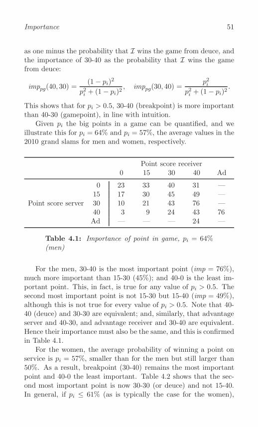
Importance 51
as one minus the probability that I wins the game from deuce, andthe importance of 30-40 as the probability that I wins the gamefrom deuce:
imppg(40, 30) =(1− pi)
2
p2i + (1− pi)2, imppg(30, 40) =
p2ip2i + (1− pi)2
.
This shows that for pi > 0.5, 30-40 (breakpoint) is more importantthan 40-30 (gamepoint), in line with intuition.
Given pi the big points in a game can be quantified, and weillustrate this for pi = 64% and pi = 57%, the average values in the2010 grand slams for men and women, respectively.
Point score receiver0 15 30 40 Ad
0 23 33 40 31 —15 17 30 45 49 —
Point score server 30 10 21 43 76 —40 3 9 24 43 76Ad — — — 24 —
Table 4.1: Importance of point in game, pi = 64%(men)
For the men, 30-40 is the most important point (imp = 76%),much more important than 15-30 (45%); and 40-0 is the least im-portant point. This, in fact, is true for any value of pi > 0.5. Thesecond most important point is not 15-30 but 15-40 (imp = 49%),although this is not true for every value of pi > 0.5. Note that 40-40 (deuce) and 30-30 are equivalent; and, similarly, that advantageserver and 40-30, and advantage receiver and 30-40 are equivalent.Hence their importance must also be the same, and this is confirmedin Table 4.1.
For the women, the average probability of winning a point onservice is pi = 57%, smaller than for the men but still larger than50%. As a result, breakpoint (30-40) remains the most importantpoint and 40-0 the least important. Table 4.2 shows that the sec-ond most important point is now 30-30 (or deuce) and not 15-40.In general, if pi ≤ 61% (as is typically the case for the women),

52 Analyzing Wimbledon
Point score receiver0 15 30 40 Ad
0 29 35 33 21 —15 25 35 43 36 —
Point score server 30 17 30 48 64 —40 7 16 36 48 64Ad — — — 36 —
Table 4.2: Importance of point in game, pi = 57%(women)
then 30-30 is the second most important point, but if pi > 62%(as is typically the case for the men), then 15-40 is second mostimportant.
The closer pi is to 50%, the less extreme are the importancevalues. When pi = 64% the importance ranges from 3% to 76%;when pi = 57% it ranges from 7% to 64%.
Big games in a set
The importance of games in a set is more complicated than of pointsin a game, because in a game we need only one probability but in aset we need two. In Tables 4.3 and 4.4 we assume that both players
Game score j0 1 2 3 4 5 6
0 30 30 18 14 3 1 —1 30 33 33 17 12 1 —2 30 33 37 37 14 8 —
Game score i 3 14 32 37 42 42 9 —4 10 12 36 42 50 50 —5 1 6 8 41 50 50 506 — — — — — 50 100
Table 4.3: Importance of game in set, gi = gj =81.3% (men)

Importance 53
are equally strong (pi = pj), so that they have the same chanceof winning a point on service. This obviously implies that theyhave the same chance of holding their service games (gi = gj). Inparticular, we choose gi = gj = 81.3% (corresponding to pi = pj =64% used earlier) for the men, and gi = gj = 67.0% (correspondingto pi = pj = 57%) for the women.
There are two types of sets: those with a tiebreak and thosewithout a tiebreak. The two tables concern sets with a tiebreak.Player I serves first in the set.
The most important game is clearly the tiebreak with imp =100% followed by any other game at the end of a set, from 4-4onwards. The score 0-0 is less important than 1-1, which is lessimportant than 2-2, and so on, until 4-4. This is because at thebeginning of a set there is more time to repair the loss of a game.
Game score j0 1 2 3 4 5 6
0 26 26 20 16 7 2 —1 26 29 29 21 15 4 —2 25 29 33 33 20 11 —
Game score i 3 16 27 33 39 39 17 —4 11 15 30 39 50 50 —5 2 7 11 34 50 50 506 — — — — — 50 100
Table 4.4: Importance of game in set, gi = gj =67.0% (women)
For the women, Table 4.4 looks similar to Table 4.3, except thatnumbers on or close to the diagonal — such as 0-0, 3-2, or 3-4 —are smaller for the women than for the men, and that the oppositeis true for numbers away from the diagonal — such as 4-1 and 2-4.This is because the probability of winning a service game is smallerfor the women than for the men. As a consequence, if the score isclose, say 1-1, then a break is more serious for the men than for thewomen, and hence close scores are more important for men thanfor women. On the other hand, if the score is not close, say at 4-1,then the woman trailing still has a chance, more than a man would

54 Analyzing Wimbledon
have, and such a game is therefore more important for women thanfor men.
The vital seventh game
Another ‘idee recue’ of commentators, and even of some players, isthe mystery of the seventh game.
Hypothesis 4: The seventh game is the most important game inthe set.
This fixation has existed for a long time, but it became popularwith Dan Maskell, BBC tennis commentator for many years and the‘voice of Wimbledon’ until he retired in 1991. He considered theseventh game ‘all-important’ and ‘vital’. However, it appears fromTables 4.3 and 4.4 that there is nothing special about the seventhgame. The score 3-3 is less important than 4-4, and 3-3 is equallyimportant as 4-3. At 4-2, importance is lower than at 3-2 and 2-2.
Before rejecting the hypothesis, let us consider it more care-fully. How would we define the importance of, say, the third game?The third game could be either at 2-0, 1-1, or 0-2. One of thesethree scores must occur in a set, but they do not occur with equalprobabilities. The probabilities can be computed from the binomialprobability function, which we already encountered on page 26. Thescore 2-0 occurs if player I holds service and breaks J . Assumingagain equal probabilities gi = gj = 81.3% of winning a service gamefor the men, the probability of 2-0 is equal to gi × (1− gj) = 15%.The same probability applies to 0-2. However, for 1-1 we obtain
gi × gj + (1− gi)× (1 − gj) = 70%,
so that 1-1 is more likely than 2-0 and 0-2. If we are in the thirdgame, we thus know the probability of each score, and for each scorewe know its importance impgs from Table 4.3. The importance ofthe third game is then given by the expected value of impgs overall three scores, that is,
impgs(3) = 0.15 × 0.30 + 0.70× 0.33 + 0.15 × 0.18 = 30%.
Likewise, the ninth game can be either at 5-3, 4-4, or 3-5. If theninth game occurs, the probability of 5-3 and 3-5 is 28% and theprobability of 4-4 is 44%, from which we compute impgs(9) = 36%.

Importance 55
But this is not the whole story. It only shows that the ninthgame is more important than the third if there is a ninth game.However, the ninth game need not occur in a set, in contrast tothe third. This matters, as the tiebreak exemplifies: conditional onits occurrence, the tiebreak is the most important game of all withimpgs(13) = 100%. Apparently the conditional concept impgs doesnot yet fully cover the idea of importance contained in hypothe-sis 4. We should account for the fact that some games occur lessfrequently than others.
Thus, let �(n) be the probability that the nth game occurs.Clearly, �(3) = 100%, but �(9) is smaller than 100%: �(9) = 84%.The unconditional importance that we require for the seventh-gamehypothesis is then given by
impgs(3)× �(3) = 0.30 × 1.00 = 30%,
impgs(9)× �(9) = 0.36 × 0.84 = 30%.
Game number n1 · · · 6 7 8 9 10 11 12 13
MenConditional 30 · · · 30 31 32 36 50 50 50 100Prob. n occurs 100 · · · 100 99 94 84 61 33 33 23Unconditional 30 · · · 30 30 30 30 30 16 16 23
WomenConditional 26 · · · 26 27 29 35 50 50 50 100Prob. n occurs 100 · · · 100 98 90 75 52 26 26 15Unconditional 26 · · · 26 26 26 26 26 13 13 15
Table 4.5: Importance of game number in set
Table 4.5 gives the values for each game number in a set, stillbased on equal probabilities of winning a service game (81.3% formen and 67.0% for women). It gives the conditional importance,impgs(n); the probability of reaching the nth game, �(n); and theunconditional importance that we need for the current hypothesis,impgs(n)× �(n).

56 Analyzing Wimbledon
It is now clear that there is nothing special about the seventhgame. The conditional importance slowly increases with the gamenumber from 30% (26% for the women) in the first game to 100%in the tiebreak. But if we take into account that the higher gamenumbers occur less frequently (for the men, 23% of the sets go toa tiebreak; 15% for the women), then there is still no special rolefor the seventh game. The three highest game numbers 11–13 arethe most important if they occur, but since they do not occur thatoften, their unconditional importance is relatively small.
Big sets
To complete the three-step analysis (point-game, game-set, set-match), we consider the importance of a set in a match. We stillassume that both players I and J have equal strength, so for eachplayer the probability si to win the set is 50%. The importanceimpsm is given in Table 4.6.
Men Women
Set score j Set score j0 1 2 0 1
0 38 38 25 50 50Set score i 1 38 50 50 50 100
2 25 50 100 — —
Table 4.6: Importance of set in match, si = 50%
In a best-of-three-set match, the importance is either 50% (at0-0, 1-0, or 0-1) or 100% (at 1-1). The same applies to a best-of-five-set match if the first two sets have been shared, because at 1-1the match becomes the same as a best-of-three match at 0-0.
At this point we need some new notation. We have used thenotation gi(a, b) to denote the probability that I wins the gamefrom the point score a-b, assuming implicitly that I is serving.Similarly, we now let mi(a, b) denote the probability that I winsthe match at the set score a-b (with point and game scores bothat 0-0). Whether I or J serves first in the match is not relevant.

Importance 57
What we earlier called mi at the beginning of the match is thus thesame as mi(0, 0). (A list of all symbols used in the book is providedin Appendix B.)
The new elements in a best-of-five match concern 0-0, 1-0, 2-0, 0-1, and 0-2. Let us examine the importance of the third setat 2-0 in sets. If I wins the set, he automatically wins the match,formalized by mi(3, 0) = 100%. If I loses the set, the score becomes2-1, and he can win the match by winning the fourth set (withprobability 50%) or by losing the fourth and winning the fifth set(with probability 0.5 × 0.5 = 25%). Hence, mi(2, 1) = 75%. Theimportance is
impsm(2, 0) = mi(3, 0) −mi(2, 1) = 100% − 75% = 25%.
The importance at 0-2 is the same, because
impsm(0, 2) = mi(1, 2) −mi(0, 3) = 25% − 0% = 25%.
The equality impsm(2, 0) = impsm(0, 2) no longer holds when theplayers differ in strength. If I is stronger than J , so that si > 0.5,then mi(2, 1) > 75% and mi(1, 2) > 25%, implying
impsm(2, 0) < impsm(0, 2).
The third set is thus more important (for both players!) if theweaker player has won the first two sets than if the stronger playerhas won them. Similarly, the second set is more important if theweaker player leads than if the stronger player leads.
Are all points equally important?
One sometimes hears that
Hypothesis 5: All points are equally important.
This is not true. Consider, for example, the famous match be-tween John Isner and Nicolas Mahut, analyzed on pages 24–27. Is-ner won the match but scored twenty-four points fewer than Mahut.This can only happen if points are not equally important. Impor-tance varies across points. Big points do exist.
We can say more by using the concept of importance. In a game,breakpoint is a more important point than 40-0. Games at the end
58 Analyzing Wimbledon
of a set are more important than at the beginning. The final set ismore important than the first set.
We have defined the importance of a point in a game (imppg),of a game in a set (impgs), and of a set in a match (impsm). Thesedefinitions and the rules of conditional probability now imply thatthe importance of a point in a match (imppm, also written simplyas imp) can be expressed as
imp = imppm = imppg × impgs × impsm.
This is convenient, because the complicated importance of a pointin a match can thus be calculated as the product of three muchless complicated importance measures. We have seen that there issubstantial variation in the values of these importance measures,and hence there is also substantial variation in the importance of apoint in a match. This confirms our rejection of hypothesis 5.
The most important point
What then is the most important point in a match? Matchpointperhaps? Usually not. For example, matchpoint at 2-0, 5-0, 40-0 isnot important at all, because even if player I loses that point, hewill almost certainly win the match. On the other hand if we are inthe tiebreak of the final set (2-2 for the men and 1-1 for the women)with a score of 6-5 or 5-6, then matchpoint will be an importantpoint.
The most important point is the point where the swing betweenwinning the point and losing it is largest. Points at the end of atiebreak have this property. Also breakpoints are important, asTables 4.1 and 4.2 show. So we expect high importance values forbreakpoints, particularly in the final set.
Table 4.7 confirms this qualitative analysis. It reports the im-portance imp of various points in a match when I is serving, againtaking pi = pj = 64% for the men and pi = pj = 57% for thewomen. The final set has a tiebreak, as at the US Open. Break-point in the final set at 5-4, 30-40 has an importance of 38% for themen (0.76 × 0.5 × 1 = 0.38). This is about three times as impor-tant as matchpoint at 5-4, 40-30 (imp = 12%), and it is also moreimportant than the points in the fourth-set tiebreak. Points in afinal-set tiebreak and breakpoints towards the end of the final set

Importance 59
Men Women
Game Point Set score Set scorescore score 2-2 2-1 1-1 1-0
6-6 6-5 50 25 50 256-6 5-6 50 25 50 255-4 40-30 12 6 18 95-4 30-40 38 19 32 164-5 40-30 12 6 18 94-5 30-40 38 19 32 16
Table 4.7: Importance of point in match, pi = pj =64% (men) and 57% (women)
are therefore the most important points in a match. Comparingmen and women in the table, we see that the ordering of the impvalues is the same, but the values themselves are not, because thepoint probability p is higher for men than for women.
Do men play more or fewer important points than women in amatch? To answer this question we need to realize that the resultsin Table 4.7 are conditional on the occurrence of an important point.Women will play more final sets than men, because the women playbest-of-three sets and the men best-of-five. But the men encounterimportant points more frequently if they play a final set, becausebreak chances occur less frequently, so that if they occur they aremore important. Similar to the result concerning long matches onpage 25, these two effects roughly offset each other: men and womenplay about the same number of important points.
Three importance profiles
We now consider the full sequence of points for the same threematches as in the previous chapter, this time not from the viewpointof forecasting but from the viewpoint of importance. In each ofthe three matches the biggest (most important) point occurs atbreakpoint towards the end of the final set. The biggest point of allis breakpoint in the fifth set of the 2008 Wimbledon final betweenRoger Federer and Rafael Nadal with an importance of 42.2%.

60 Analyzing Wimbledon
Federer-Nadal
In the 2008 Wimbledon final, Roger Federer was defeated by RafaelNadal in five sets: 4-6, 4-6, 7-6, 7-6, 7-9. A total of 413 points wereplayed. Figure 4.1 confirms the large variation in importance acrosspoints. Eighty of the points had imp > 10 and four really big pointshad imp > 40, all in percentages.
Importance
50 100 150 200 250 300 350 400 0
10
20
30
40 set 1 set 2 set 3 set 4 set 5
Point number
Figure 4.1: Importance profile, Federer-Nadal,Wimbledon 2008
In the first set, there were breakpoints at 1-1 and 1-2, and twofurther breakpoints at 4-5. At 4-5, Nadal served for the set andFederer had two breakpoints to level at 5-5 (imp = 15.4). Nadal’ssetpoints (imp = 4.0) were less important than Federer’s break-points. In the second set there were breakpoints at 4-2, 4-3, 4-4,and 4-5, all visible in the figure. In both sets, Nadal was serving forthe set at 4-5, and in both cases Federer had breakpoints. In thefirst set, the importance of the breakpoint was 15.4; in the secondset 16.5. This is because the second set is more important than thefirst when the underdog (Nadal in this case) wins the first set; seethe discussion on page 57.

Importance 61
The only big point in the third set occurred at 6-5 in the tiebreakwith Federer serving for the set (imp = 14.0). Many big pointsoccurred in the fourth-set tiebreak: at 5-5 and 7-7 with Federerserving (imp = 27.1) and at 6-6 and 8-8 with Nadal serving (imp =26.7). Nadal’s points are slightly less important than Federer’sbecause if Nadal loses his service point it is likely that he loses theset but not necessarily the match, while if Federer loses his servicehe will likely lose the match. There are two setpoints for Federer(imp = 26.3) and two matchpoints for Nadal (imp = 27.5).
In the fifth set the importances are higher overall than in thefourth, corresponding to the larger shocks in the forecasting profilein the fifth set compared to the fourth (Figure 3.1). The breakpointat 4-3 on Nadal’s service has imp = 32.8. But the four really bigpoints all occur later in the fifth set, all on Federer’s service: thebreakpoint at 5-5 and three further breakpoints at 7-7 (imp = 42.2).Having broken at 7-7, Nadal serves for the match. Matchpoint(imp = 11.0) is rather less important than many of the previouspoints.
Clijsters-Williams
The semi-final at the 2010 US Open between Kim Clijsters andVenus Williams was won by Clijsters in three sets: 4-6, 7-6, 6-4.Of the 191 points played, there were 32 points with imp > 10,3 of which with imp > 20. In the first set, the biggest point wasbreakpoint at 3-3 on Clijsters’ service (imp = 11.9), which Williamswon, going on to win the set. This is visible in Figure 4.2 as thehighest dot in the first set. The second-set tiebreak produced thebig points in the second set, interestingly at the beginning (0-0 and1-0). The tiebreak went to 4-0 and 7-2, not producing any otherbig points.
In total there were nine points with imp > 15, all in the thirdset. Early in the third set there were breakpoints on Clijsters’service at 0-1 (imp = 17.3) and at Williams’ service at 1-1 (imp =15.8). The three biggest points occurred at 4-3 when Williams hada breakpoint (imp = 22.2), and at 4-4, Williams serving, at 30-30(imp = 23.6) and at breakpoint (imp = 28.0). At 5-4 Clijsterswon her first matchpoint at 40-15, but this was not a big point(imp = 6.8).

62 Analyzing WimbledonIm
portance
20 40 60 80 100 120 140 160 180 0
10
20
30set 1 set 2 set 3
Point number
Figure 4.2: Importance profile, Clijsters-Williams,US Open 2010
Djokovic-Nadal
Finally we reconsider the 2012 final at the Australian Open, whereNovak Djokovic defeated Rafael Nadal in five sets: 5-7, 6-4, 6-2,6-7, 7-5. The importance profile, shown in Figure 4.3, provides theimportance of each of the 369 points played. Fifty-six points had animportance of imp > 10, sixteen of imp > 20, and four of imp > 30.Two big points occurred in the fourth-set tiebreak, and all otherbig points occurred in the fifth set. There were breakpoints at 2-3(imp = 27.6) and at 2-4 (imp = 26.2). The biggest points occurredat 4-4 and 5-5, Nadal serving, breakpoint to Djokovic (imp = 34.7),and at 6-5, Djokovic serving, breakpoint to Nadal (imp = 34.6).
Further reading
The seminal paper on importance in tennis is Morris (1977), andour definition and several other issues in the current chapter buildon this paper. Morris also notes that the aggregate importance of

Importance 63Im
portance
50 100 150 200 250 300 350 0
10
20
30
set 1 set 2 set 3 set 4 set 5
Point number
Figure 4.3: Importance profile, Djokovic-Nadal,Australian Open 2012
all points served to the deuce court equals that for the ad court.Because more points are served to the deuce court, higher averageimportance is experienced in the ad court. This is one reason fordouble teams to have the player who performs best at importantpoints receive on the left side.
Another notable result is that the player who serves first in aset serves in the less important games. This does not imply thatserving first is an advantage in the sense that the server wins his orher games more easily. In Chapter 11 we will test whether such anadvantage exists. If it does exist, then it could possibly be explainedby the reduced importance and pressure.

This page intentionally left blank

5Point data
So far we have used very few data and no statistical techniques; wehave relied on mathematics. If we want to prove or disprove populartennis hypotheses (e.g., ‘real champions win the big points’), findout more about the trade-off between first and second service, ordetermine whether ‘momentum’ or ‘winning mood’ exist in tennis,then we need to apply statistical techniques. But before we canapply these techniques we need data.
We shall use various data sets, some recent, some less recent.In this chapter we describe a Wimbledon data set at point levelover four years, 1992–1995. This will be our main data source. Itis a rich source covering many different players. But it is not theindividual players that we are primarily interested in. Our interestis in professional tennis in general, and the Wimbledon data setwill teach us many lessons about professional tennis. An obviousconcern is whether these relatively old data are still of interest to-day. We shall study and comment on the changes over time, usingother data sets, and conclude that our Wimbledon data set is stillremarkably relevant.
The Wimbledon data set
Our data set consists of 481 matches (88,883 points) played in themen’s singles and women’s singles at Wimbledon from 1992 to 1995.This accounts for almost half of all singles matches played duringthe four years, as only matches on one of the five ‘show courts’were recorded (the show courts are the courts where the matcheswith the best-known players are typically scheduled). For each of

66 Analyzing Wimbledon
these matches we know the players, their rankings, and the exactsequence of points. We also know at each point whether or nota second service was played and whether the point was decidedthrough an ace or a double fault.
Men Women
Matches 258 223Sets 950 503Final sets 51 57Games (excl. tiebreaks) 9367 4486Tiebreaks 177 37Points (incl. those in tiebreaks) 59, 466 29, 417Points (excl. those in tiebreaks) 57, 319 28, 979
Table 5.1: Wimbledon data set: totals, 1992–1995
Table 5.1 provides a summary of the data. We have slightlymore matches for men (258) than for women (223), but of coursemany more sets, games, and points in the men’s singles than inthe women’s singles, because men play best-of-five sets and womenbest-of-three. Almost 60,000 points are observed in the men’s sin-gles and almost 30,000 in the women’s singles. The men’s singles aretherefore seriously overrepresented on the show courts, and abouttwo-thirds of the spectators’ viewing time goes to the men. If sexequality in viewing time would be a goal, The All England LawnTennis and Croquet Club should aim for 193 matches (a 25% reduc-tion) in the men’s singles and 335 matches (a 50% increase) in thewomen’s singles on the five show courts. (In Wimbledon’s defense:a slightly smaller adjustment will achieve equality in viewing time,due to the fact that women play longer rallies than men.)
Table 5.2 presents proportions associated with the totals in Ta-ble 5.1. The men play on average 231 points per match, the women132, and hence a match in the men’s singles takes on average 1.75times as long (in terms of points) as a match in the women’s singles.
Both men and women play about the same number of pointsper set, around sixty. Because the men have a higher probabilityof winning a service point than the women, the men play fewerpoints per game than the women, but they play more games per

Point data 67
Men Women
Sets in match 3.7 2.3Games in set 9.9 8.9Games in match 36.3 20.1Tiebreaks in (non-final) set 0.2 0.1Tiebreaks in match 0.7 0.2Points in game 6.1 6.5Points in tiebreak 12.1 11.8Points in set 62.6 58.5Points in match 230.5 131.9
Table 5.2: Wimbledon data set: proportions,1992–1995
set. These two opposite forces appear to be approximately equal,resulting in approximately the same number of points per set. Inaddition, the quality difference in the men’s singles is smaller thanin the women’s singles, as discussed on page 24: scores like 6-0 and6-1 are more common for the women than for the men. This is whythere are more tiebreaks per set for men than for women.
The original data set was of high quality with very few errors.Still, after performing all possible checks, we had to delete about4% of the matches, which contained non-repairable errors or hadnot been completed. The remaining 481 matches constitute ourdata set — they passed all our tests and are therefore ‘error-free’.For a statistician, having a large, detailed and error-free data set isan exceptional and happy situation. In most studies the reliabilityof the data is a serious concern, but in sport statistics the data aretypically of very high quality, allowing better analysis and sharperconclusions.
Two selection problems
All matches in our data set are played on one of the five show courts:Centre Court and courts 1, 2, 13, and 14 at the time. Becausetop players are typically scheduled on these courts, this causes anunderrepresentation in the data set of matches involving non-seededplayers. This is a problem, a so-called selection problem.

68 Analyzing Wimbledon
It is not the only selection problem. If two non-seeded playersmeet in the quarter-final, then this match is likely to be scheduledon a show court. But, if they play each other in the first round, theirmatch is considered to be less important and is likely to be playedon another court. After all, there are sixteen first-round matchesinvolving a seeded player and such matches typically take prece-dence. (In the period 1992–1995, sixteen players were seeded; from2001 onwards, thirty-two.) The underrepresentation of matches be-tween two non-seeded players is therefore most serious in the earlyrounds. This dependence on round in the selection of matches isalso present in other types of matches (seeded versus non-seeded orseeded versus seeded), but there the problem is less serious.
Sd-Sd Sd-NSd NSd-NSd Total
Round S P S P S P S P
Men1 — — 48 64 34 192 82 2562 — — 46 54 16 74 62 1283 — — 39 41 16 23 55 644 (last 16) 8 9 15 15 8 8 31 325 (quarter) 7 7 9 9 0 0 16 166 (semi) 7 7 1 1 0 0 8 87 (final) 4 4 0 0 0 0 4 4Total 26 27 158 184 74 297 258 508
Women1 — — 43 63 24 193 67 2562 — — 43 58 3 70 46 1283 — — 42 48 12 16 54 644 (last 16) 8 8 20 21 2 3 30 325 (quarter) 11 12 3 3 1 1 15 166 (semi) 6 6 1 2 0 0 7 87 (final) 4 4 0 0 0 0 4 4Total 29 30 152 195 42 283 223 508
Table 5.3: Matches between seeded (Sd) and non-seeded (NSd) players in the sample (S) and in thepopulation (P)

Point data 69
Table 5.3 provides more details about both selection problems.We distinguish between round (1 = first round, . . . , 7 = final) andtype of match (Sd-Sd for two seeded players, Sd-NSd for a seededagainst a non-seeded player, and NSd-NSd for two non-seeded play-ers). The columns labeled ‘S’ contain the number of matches inour sample, and the columns labeled ‘P’ give the number of allmatches played (matches in the population). In the first roundof the women’s singles there are sixty-three rather than sixty-fourmatches between a seeded and a non-seeded player. This is becauseMary Pierce, seeded 13, withdrew in 1993 at the last moment. Shewas replaced by Louise Field, an unseeded player.
The percentage of matches involving two non-seeded players(NSd-NSd) in our data set is 24.9 (74/297) for the men and 14.8(42/283) for the women. Both are lower than the percentages forSd-NSd matches, which are themselves lower than those for Sd-Sdmatches. This illustrates the first selection problem: the underrep-resentation of matches involving non-seeded players.
Round dependence, the second selection problem, is caused bythe increasing sampling percentages over the rounds. For example,only 32.0% (82/256) of all first-round matches in the men’s singlesand 26.2% (67/256) in the women’s singles are in the data set,whereas all finals have been sampled.
Since we wish to make statements about Wimbledon in gen-eral, and not just about the matches in our sample, we account forboth selection problems by weighting the matches when computingstatistics. The weight of a match is the ratio P/S using the popula-tion and sample values in Table 5.3 for the round and type of match.The validity of this procedure involves an assumption, namely thatthe decision by Wimbledon’s organizers whether a match in one cellis on a show court or not is random within that cell, so that thematches on the show courts (which are the matches we observe) arerepresentative.
One could argue that, if the sample is very small compared tothe population, this method would make the few observed matchestoo important. Most notably, in the women’s singles we observeonly three of the seventy matches played between two non-seededplayers in the second round. If these three matches were selectedby the organizers to include, for example, players just outside thetop sixteen, then our method would be seriously biased for this

70 Analyzing Wimbledon
cell. As it happens, the three matches concern players with WTArankings 27-41, 131-143, and 22-113, and hence there is no reason tobelieve that these matches are not representative. Still, in the moreadvanced analyses from the next chapter onwards we combine thethree women’s matches in the second round with the twenty-fourmatches in the first round, and weight all twenty-seven matches by263/27.
We have experimented with other weighting methods, and wefind that our results are not sensitive to the method of weighting.Whenever the Wimbledon data set is used in this book, we shalluse the above weights to make the sample more representative andwe shall call the weighted data set simply ‘the data set’.
Estimators, estimates, and accuracy
One concern with our detailed data set is that it is relatively old.We consider the years 1992–1995 and one may wonder whetherthese data are still of interest today. Has tennis not changed? Thisis a reasonable concern and we need to address it.
We start by considering p, the probability of winning a servicepoint. This was the key probability in previous chapters, where weallowed it to differ across players, reflected in the notation pi. Inthe following chapters we will again differentiate between players,for example by introducing a player’s ‘quality’ in Chapter 7. But inthe current chapter we simply put all players together. Hence thereis one single p for the men and one single p for the women, reflectingthe service strength of professional tennis players in general.
The value of p is not observable. To estimate it we need dataand a bit of statistical theory. Suppose there are T service pointsin the sample. Some of these T points will be won by the server(successes), the other points by the receiver. A natural estimatorof the unknown probability of success p is the observed relativefrequency of successes:
p =number of service points won by server
total number of service points in the sample,
where the hat above p signifies that we are dealing with an esti-mator. We have T = 59, 466 for the men and T = 29, 417 for the

Point data 71
women, and we obtain p = 64.4% and p = 56.1%, respectively. Notsurprisingly, men win more points on service than women.
To be precise: an estimator is a formula, like the formula forp above. An estimate is the realization of the formula when wesubstitute numbers for symbols. So, the realizations p = 64.4%and p = 56.1% are estimates, not estimators.
This estimator of p is a good estimator in the sense that onaverage it produces the right answer. We express this by sayingthat the expected value of p is equal to the true value: E(p) = p.But this is only on average. There will be deviations from theaverage, p−E(p), and the variation of p is usually expressed as thevariance,
var(p) = E (p− E(p))2 .
To compute the variance, we put all players together (only in thischapter). This means that we assume that all points are iid, notonly within players (as in hypothesis 1), but also between players.It is doubtful whether the latter part of the assumption is realistic,and we shall return to it in the next chapter. Assuming that bothparts of the assumption are satisfied, the variance can be computedas var(p) = p(1 − p)/T . The higher is T , the lower is var(p), thecloser is p to the true value p, and the more accurate is p.
Since the variance involves the square of p, we typically take thesquare root of the variance in order to obtain a measure in the samescale as p. The estimate of this square root is called the standarderror, written as ‘se’. To quantify the inaccuracy of the estimatewe thus take
se =√
p(1− p)/T ,
where we have substituted the unknown p by its estimate. Inour case the standard errors are se = 0.2% (men) and se = 0.3%(women), smaller for the men than for the women, mainly becausewe observe more points for the men.
The estimation results are then summarized as
p =
{64.4% (0.2%) for the men,
56.1% (0.3%) for the women.
Under certain conditions, which are typically assumed to hold, theinterval defined by the estimate ± twice the standard error cov-ers 95% of the possible outcomes of the estimator. This means,

72 Analyzing Wimbledon
loosely speaking, that we expect p to lie between 64.0% and 64.8%for the men and between 55.5% and 56.7% for the women. Theseuncertainty intervals are called ‘confidence intervals’. The confi-dence intervals are quite narrow here, reflecting the precision of ourestimates, caused by the fact that we have many observations. Sta-tistical theory has thus helped us to learn about the magnitude ofsomething unobservable, the probability of service success, as wellas about the accuracy of that information.
Development of tennis over time
To answer the question of whether the point data are still of interesttoday, we study the two relative frequencies 64.4% (men) and 56.1%(women) in some more detail. How stable are these estimates overtime?
Men Women
1992 64.9 (0.4) 57.0 (0.6)1993 64.9 (0.4) 56.6 (0.6)1994 63.9 (0.4) 55.4 (0.6)1995 64.0 (0.4) 55.4 (0.5)
Table 5.4: Percentage of points won on service,1992–1995
Table 5.4 presents the development of p during our observationperiod. The numbers in brackets denote again the standard errorsof the estimators. The estimates suggest that service dominancehas decreased somewhat between 1992 and 1995, both for men andfor women, presumably not because the service has weakened butbecause the return of service has improved. However, a value of,say, 64.5% lies within all four uncertainty intervals for the men, sothat the true p may in fact have been constant over the years. Inthat case, the decrease in the service dominance may be spuriousand could just be a coincidence. The same holds for, say, 56.0% inthe women’s singles.
Has this (possible) decrease of the service dominance continued?Using totals over all Wimbledon matches from 1992 until 2010 (in-

Point data 73
1995 2000 2005 2010 0
20
40
60
80
100
1995 2000 2005 2010 0
20
40
60
80
100
Figure 5.1: Service dominance, 1992–2010 (menleft, women right)
formation that is not in our main data set), we plot the estimatedvalue of p in Figure 5.1. There is no indication of a further decreasein service dominance. The probability of winning a service pointappears to be remarkably stable over the years.
1995 2000 2005 201050
55
60
65
70
1995 2000 2005 201050
55
60
65
70
Figure 5.2: Service dominance, 1992–2010, zoomedin (men left, women right)
Zooming in on Figure 5.1 produces Figure 5.2. Here some moredetail is visible, including the 95% uncertainty bounds. The proba-bilities are still quite stable, and there is no indication of a furtherdecrease of service dominance. If anything, it appears that the ser-vice dominance is increasing from 2003 onwards for the men, andfrom 1995 onwards for the women, but the evidence is not strong.
The 1992–1995 data are therefore quite informative about tennisin later years, at least regarding the probability p of winning apoint on service. This does not mean that tennis has been stablein every dimension. For example, there has been a decline of serve-and-volley tennis — the grass remains greener near the net during

74 Analyzing Wimbledon
Wimbledon — but this has not coincided with a drop in servicedominance p. Maybe the service has become more powerful. Ifso, then the return of service has also improved, and both effectsapparently offset each other.
Winning a point on service unraveled
The service is one of the most important aspects of tennis, partic-ularly on fast surfaces such as the grass courts at Wimbledon. Sofar we have only discussed the probability p of winning a point onservice. But tennis has two serves, and therefore more informationcan be obtained from the data.
Men Women
1st service in 59.4 (0.2) 60.8 (0.3)2nd service in 86.4 (0.2) 86.0 (0.3)Points won if 1st service in 73.3 (0.2) 62.2 (0.4)Points won if 2nd service in 59.4 (0.3) 54.1 (0.5)Points won on 1st service 43.6 (0.2) 37.8 (0.3)Points won on 2nd service 51.4 (0.3) 46.6 (0.5)Points won on service 64.4 (0.2) 56.1 (0.3)
Table 5.5: Service percentages
The principal service characteristics are provided in Table 5.5.Some of these characteristics are typically also shown on television,although they are sometimes called differently. For example, thecommonly presented ‘winning % on 1st serve’ and ‘1st serve pointswon’, two names for the same statistic, are what we call ‘pointswon if 1st service in’, which is a more accurate description. Whatwe call ‘points won on 1st service’ is the percentage of 1st serviceshit that have resulted in winning the point. This corresponds tothe earlier definition of ‘points won on service’ (the percentage ofpoints served that have resulted in winning the point).
The characteristic that is typically not shown on television is‘points won on 1st (or 2nd) service’. This is remarkable, because itis precisely this probability that is of most interest. After all, almostanyone (even amateur players) can achieve a ‘1st (2nd) service in’

Point data 75
percentage of close to 100%, although such a service would be tooeasy for the receiver and therefore not optimal. Most professionalplayers can also achieve a high percentage on ‘points won if 1st(2nd) service is in’, by making the service very risky, so that it is afault most of the time, but if it goes in, it will have a high chanceof winning the point. Both probabilities are typically presentedon television. But it is not the two probabilities themselves thatmatter most — it is their product. As a result, the percentage‘points won on 1st (or 2nd) service’ provides a proper measure ofthe dominance of the first (second) service.
In the men’s singles, on average, the first service is in 59.4% ofthe time. If the first service is in, the probability of winning thepoint is 73.3%. The probability of winning the point on the firstservice is therefore 59.4% × 73.3% = 43.6%. In general,
% of points won on 1st service
= (% of points won if 1st service in)× (% 1st services in).
Of course, the same holds for the second service.
Combining the data for the first and second services, we can de-rive the percentage of points won on service, the correct measure ofservice dominance. A player can win a point on service in two ways:on the first or on the second service, where the second possibilityonly becomes relevant when the first serve is a fault. Therefore,
% of points won on service = % of points won on 1st service
+ (% 1st service not in)× (% of points won on 2nd service).
For example, in the men’s singles,
64.4% = 43.6% + (100 − 59.4)% × 51.4%.
The percentage of points won on the first service is plotted inFigure 5.3, where we have ‘zoomed in’ to provide more detail. Theprobabilities are quite stable, although they have risen slightly inrecent years, both for men and for women. The second-servicepercentages, presented in Figure 5.4, are even more stable over timethan the first-service percentages.

76 Analyzing Wimbledon
1995 2000 2005 201030
35
40
45
50
1995 2000 2005 201030
35
40
45
50
Figure 5.3: Percentage of points won on first service,1992–2010 (men left, women right)
1995 2000 2005 201040
45
50
55
60
1995 2000 2005 201040
45
50
55
60
Figure 5.4: Percentage of points won on second ser-vice, 1992–2010 (men left, women right)
Testing a hypothesis: men versus women
A comparison between men and women in Table 5.5 reveals —apart from the obvious differences — that the percentage of firstand second service in is almost the same. The first service is in59.4% of the time for men and 60.8% for women, while the secondservice is in 86.4% of the time for men and 86.0% for women. It isnot immediately clear why these percentages should be so close.
What do we actually mean by ‘almost the same’? To answerthis question we formulate the following hypothesis.
Hypothesis 6: The probability that the service is in is the samein the men’s singles as in the women’s singles.
To test the hypothesis we consider the difference diff1 between

Point data 77
men and women of the probability that the first service is in. Sim-ilarly, we consider the difference diff2 for the second service. If thehypothesis is true, then diff1 and diff2 are both zero. We don’tknow diff1 and diff2, but from Table 5.5 we can derive estimates ofthem, namely −1.40 and 0.38, respectively.
The fact that these numbers differ from zero does not necessar-ily mean that we reject the hypothesis. It could be pure randomnessthat has made them different from zero even though the hypoth-esis is actually true. The question is whether they are sufficientlydifferent from zero to reject the hypothesis. To understand what‘sufficiently’ means in a statistical sense, we must take the uncer-tainty of the estimates into account, and this is where we need thestandard error of the estimators. Because the men and women sam-ples are independent (an assumption made throughout this book),the variance of the estimator of diff1 (and similarly of diff2) is equalto the sum of the variance of the estimator for the men and the vari-ance of the estimator for the women. We then find from Table 5.5that
diff1 = −1.40 (0.34), diff2 = 0.38 (0.40).
Given these estimates and standard errors we can construct confi-dence intervals similar to those on page 72. In this case, the confi-dence intervals are (−2.08, −0.72) and (−0.42, 1.18), respectively.This means that with 95% certainty the data imply that the truediff1 and diff2 lie inside these intervals.
If the hypothesis were true, then we would expect that zero liesinside the interval. This is the case for the second service, andhence there is no reason to reject the hypothesis that diff2 = 0.If, on the other hand, zero lies outside the interval (as is the casefor the first service), then something is wrong. Many things couldbe wrong, but if we assume that all underlying assumptions holdexcept possibly the hypothesis, then we must conclude that thehypothesis is wrong and reject it.
Given the 95% confidence, we will incorrectly reject the hypoth-esis 5% of the time. So in 5% of the cases we reject a hypothesiswhen in fact it is true. This is the price one has to pay in hypothesistesting. All testing in the book is based on the 5% level.
Another way of saying that we reject the hypothesis, is to saythat the underlying estimate, here diff1, is ‘statistically signifi-cantly’ different from zero, in short ‘significant’. If, on the other

78 Analyzing Wimbledon
hand, zero lies inside the interval (as for the second service), thenthere is no evidence that something is wrong and we do not rejectthe hypothesis. The underlying estimate, here diff2, is then called‘insignificant’.
Insignificance does not mean that we accept the hypothesis.Statisticians always emphasize that hypothesis testing is about re-jecting or not rejecting a hypothesis, not about rejecting or accept-ing a hypothesis. This is because, if we do not reject a hypothesis,there are many possible reasons and only one reason is that thehypothesis is true. It could be, for example, that the statisticalanalysis is not powerful enough to detect deviations from the hy-pothesis even when the hypothesis is in fact false.
Hypothesis testing results in a binary outcome: rejection or norejection. This is not completely satisfactory, because a small in-crease in standard error could change the conclusion from rejectto not reject. The binary nature uses only part of the informationavailable in the data, in contrast to confidence intervals. Still, a bi-nary outcome is customary and simple, and we will use it through-out this book.
This is hypothesis testing in a nutshell. Based on our estimatesand assumptions we conclude that the probability that the firstservice is in is not the same in the men’s singles as in the women’ssingles, but that the probability that the second service is in maybe the same.
Aces and double faults
Of special interest, and always included in television statistics, arethe number of aces and double faults. The percentage of aces isdefined as the ratio of the number of aces (first or second service) tothe number of points served, rather than to the number of services.The percentage of double faults is the ratio of the number of pointswith a double fault to the number of service points.
In our Wimbledon data set, 8.2% (0.1%) of the points weredecided through an ace in the men’s singles, and 3.1% (0.1%) inthe women’s singles. It is not surprising that men serve almostthree times as many aces as women. More surprising perhaps is thestability of this percentage over time, as shown in Figure 5.5.

Point data 79
1995 2000 2005 2010 0
5
10
15
20
1995 2000 2005 2010 0
5
10
15
20
Figure 5.5: Percentage of aces, 1990–2010 (men left,women right)
1995 2000 2005 2010 0
5
10
15
20
1995 2000 2005 2010 0
5
10
15
20
Figure 5.6: Percentage of double faults, 1990–2010(men left, women right)
Figure 5.6 shows that the percentage of double faults has de-creased slightly over time for the men, which could still be dueto estimation uncertainty, but has remained stable for the women.About 5.5% of the points served result in a double fault, both forthe men and for the women. This can be deduced from Table 5.5,because{
(1− 0.594) × (1− 0.864) = 5.52% for the men,
(1− 0.608) × (1− 0.860) = 5.49% for the women.
The standard errors are 0.09% and 0.13%, respectively.
An alternative to hypothesis 6, now taking both services intoaccount, is to compare double faults.
Hypothesis 7: The probability of a double fault is the same in themen’s singles as in the women’s singles.

80 Analyzing Wimbledon
The difference in probability between men and women is esti-mated to be 0.03%-points with a standard error of 0.16%-points.Since the standard error is large relative to the estimate, the con-fidence interval (−0.29, 0.35) covers zero, so that the hypothesis isnot rejected. Therefore, it may indeed be the case that the per-centage of double faults is the same for men and women. This isa remarkable fact, which requires further investigation. Unfortu-nately, our data are not sufficiently rich to understand the under-lying cause.
Of course, players could lower the number of double faults bymaking their service easier. They don’t do this, because the prob-ability of winning a point decreases if the service is too easy. If aplayer serves no double faults in a match, this does not necessarilyshow that he or she has served well. It may well indicate that theserver has not taken enough risk at his or her service. There is anoptimal number of double faults in each match for each player, andthis optimum number is, in general, not zero.
Breaks and rebreaks
So far we have only used simple frequencies, and this has producedcredible estimates and test outcomes. But this need not always bethe case. Unexpected conclusions can emerge if we do not analyzethe data in a statistically sound manner. Consider for example thefamous break-rebreak hypothesis.
A break occurs if the server does not win his or her own servicegame. If this break does not decide the set, then the next gameis often considered special. The server in the next game can now‘confirm’ the break by holding service, or he or she can be brokenback. Some commentators believe that there is a higher probabilityof being broken back after a break, perhaps because the player whoachieved the break enjoys the success and relaxes a bit, while theopponent is eager to strike back immediately.
Hypothesis 8: After a break the probability of being broken backincreases.
If the hypothesis is true, then the probability of winning a pointon service decreases after a break in the previous game (in thesame set). Using our Wimbledon data we obtain Table 5.6. In

Point data 81
the men’s singles, 64.4% of the points are won by the server. Thewomen win fewer service points (56.1%), as we already know. If theprevious game was a break, then the probability of holding serviceis larger rather than smaller, both for men and women. And, if theprevious game was not a break, then the probability is smaller thanaverage. The difference between ‘after break’ and ‘after no-break’is 1.7%-points (men) and 3.0%-points (women), respectively. Bothestimates are significant.
Men Women
All points 64.4 (0.2) 56.1 (0.3)After break 65.8 (0.5) 57.9 (0.5)After no-break 64.1 (0.2) 54.9 (0.4)
Table 5.6: Percentage of winning a point on serviceafter winning or losing the previous game
If we translate these percentages from points to games, then wefind that the probability of winning a service game is 3.3%-pointshigher if a break occurred in the previous game than if no breakoccurred. This is for the men; for the women the difference is 5.7%-points.
It seems therefore that the hypothesis is wrong. The oppositeis true. But is this a credible conclusion? For example, should wenot allow for quality differences between players? If the top seedplays against a relatively weak player and wins 6-0, 6-0, 6-0, thenthere are many breaks but no rebreak, not because the hypothesisis wrong, but because the top seed is a much better player. The‘after break’ winning probability is thus dominated by good playersand therefore higher than the ‘after no-break’ winning probability,which is dominated by weaker players. Quality heterogeneity canexplain a positive difference, even when a break in the previousgame does not matter at all.
This is an example of a well-known issue in statistics calledsample selection bias: players are not randomly selected into thesample used to estimate a probability and this biases the estimators.Sample selection bias matters for many simple statistical analyses,also in this book. Sometimes the impact is small, sometimes it is

82 Analyzing Wimbledon
big. The problem is that we do not know this beforehand. We shallreturn to the break-rebreak hypothesis and investigate the effectof sample selection bias in Chapter 12, after we have developed astatistical model that properly handles quality differences to avoidthe bias.
Are our summary statistics too simple?
One of the purposes of this little book is to show that sometimesa simple statistical analysis suffices, and sometimes not. In thebreak-rebreak case, the analysis is ‘too simple’. To find the precisebalance between complexity and simplicity is the art of modeling.
This chapter has introduced our data set and we have performedsome simple averaging exercises. Two things, in particular, wereignored: clustering and quality. We have treated every point thesame, while in fact the points are clustered in matches and, withina match, in players. Each player has his or her own underlyingprobabilities and the performance of one player depends on the op-ponent in the match. Moreover, the differences between players arenot random. Some have a higher ranking than others and we wantto exploit such observable information in order to obtain better es-timates. How do we allow for these quality differences? And, moredifficult, how do we allow for unobservable quality differences, suchas form of the day? Chapter 6 will deal with the clustering issue;the quality correction is discussed in Chapter 7.
Further reading
Summary statistics are often presented on television. Bedford et al.(2010) discuss many variants and their interpretations. They alsoshow how summary statistics vary across surfaces. For example,both men and women win the highest percentage of service pointswhen playing on grass, followed by carpet, hard court, and clay.
O’Donoghue and Ingram (2001) examine other types of sum-mary statistics. They analyze more than three hundred hours ofgrand slam matches over the period 1997–1999, regarding the num-ber of shots per rally, rally time, inter-point time, and so on. Ralliesin men’s matches are shorter than in women’s matches, they areshortest at Wimbledon, and longest at Roland Garros. Men take
Point data 83
more time between points than women. We do not know whetherthis still holds today.
Several authors study the development and changes of tennisover time. Coe (2000) relates the changes in tennis over manydecades to technology, from rackets and balls to court surfaces.Guillaume et al. (2011) examine the careers of the top-ten menand women players between 1973 and 2009. The average careerlength is about sixteen years for both men and women. Men playtheir first match at age 17.5 and women at age 15.9. Women reachtheir highest level earlier than men, and for both men and womenthe peak performance tends to occur at a younger age now than inthe past.
Dudink (1994) studies the birthdate distribution of successfuljunior tennis players in The Netherlands. He finds that the dis-tribution is not symmetric; it is skewed, with half of the twelve-to sixteen-year-old top Dutch tennis players being born in the firstthree months of the year. This is due to the cut-off date for juniorcompetition age groups, namely 1 January. Edgar and O’Donoghue(2005) confirm this season-of-birth bias, and they find a similarpattern for senior players, using grand slam data for both menand women. Notable exceptions are Aranxa Sanchez-Vicario andRichard Krajicek, both born in December and nevertheless grandslam champions.
Finally, Radicchi (2011) estimates who is the best male playerever. He considers more than 130,000 matches between 1968 and2010 and forms a network where players are linked through matches.Jimmy Connors turns out to be the best player, justified by hisextremely long, consistent, and successful career, holding a top-tenposition for sixteen consecutive years (1973–1998).

This page intentionally left blank

6The method of moments
To make further progress we need to know more about estimationtheory. For example, we want to account for the clustering of pointsin matches and players, and this can only be achieved by intro-ducing more theory. In this chapter we introduce a much-appliedstatistical theory: the method of moments, more precisely the gen-eralized method of moments (GMM). The word ‘moments’ refers tostatistical operators, such as the expectation and the variance (firstencountered and defined on page 71). The method will handle theproblems encountered so far, it can be extended later on, and willbe used extensively in the following chapters. We begin with thesimplest setup so that we can link the new results directly to whathas been learned in the previous chapter. Then we gradually addnew elements.
Our summary statistics are too simple
In the previous chapter all points were pooled. We distinguishedbetween men and women, but otherwise we did not distinguish be-tween matches or players. For example, the probability of winninga point on service was estimated by p, the total number of points inthe data set won on service divided by the total number of pointsserved. This simplicity may be sufficient for some purposes, butnot if we wish to dig deeper.
One problem of pooling is that all points are treated as inde-pendent and identically distributed (iid). This may be a reasonableassumption within one player within one match, and this is the con-tent of hypothesis 1. But the hypothesis does not suggest that allpoints in the data set are iid, and of course they aren’t. Points are
86 Analyzing Wimbledon
clustered in matches and, within a match, in players. Each playerhas his or her own underlying probabilities and the performance ofone player depends on the opponent in the match.
Thus motivated we now think of a match as the unit of analysis,and this necessitates a refinement of our notation. Suppose thereare N matches in our data set (N is 258 for the men and 223 for thewomen), and consider a match between two players I and J . PlayerI serves Ti points and wins a fraction fi of them. This clusters thepoints served by I. The points served by J are similarly clustered.Per match we observe two relative frequencies, fi of player I andfj of player J .
As in the previous chapter, we first focus on the probability pto win a point on service. A natural alternative to the previouslydefined estimator p, which, in contrast to p, accounts for the clus-tering, is obtained by taking the average of fi and fj in a matchand then average over all N matches in the sample. In formula,
pm =1
2N
∑(fi + fj),
where the Greek capital sigma is the mathematical symbol for thesummation operator, here over all matches.
Under appropriate assumptions, the standard error accompany-ing pm is
sem =1
2N
√∑(fi(1− fi)
Ti+
fj(1− fj)
Tj
).
What are these appropriate assumptions? The two expressionsfi(1 − fi)/Ti and fj(1 − fj)/Tj in the above formula are the es-timated variances of fi and fj, respectively. They resemble theexpression in the old variance formula p(1 − p)/T on page 71, butnow they are formulated for each player separately because we onlyassume iid for points within one player. If we ignore (for now) thecorrelation between the two opponents I and J , and if matches areuncorrelated, then the formula for the standard error is correct.
Table 6.1 presents three different estimates for the same overallprobability p (points won on service) and also for the underlyingand associated probabilities. The estimate in the column ‘point’ isobtained by taking the mean across all points. Regarding p, this

The method of moments 87
is the estimate p of Chapter 5. The second estimate is pm, whichaverages matches and players. The estimate in the GMM columnis also a match-based estimate and will be discussed later in thischapter (page 91).
Men Women
Point Match Point Matchmean mean GMM mean mean GMM
1st service (s.) in 59.4 59.4 59.4 60.8 60.5 60.5(0.2) (0.3) (0.4) (0.3) (0.5) (0.7)
2nd service in 86.4 86.6 86.4 86.0 85.9 85.7(0.2) (0.3) (0.4) (0.3) (0.5) (0.7)
Points won if 1st s. in 73.3 73.5 73.3 62.2 63.0 62.5(0.2) (0.3) (0.5) (0.4) (0.6) (0.6)
Points won if 2nd s. in 59.4 59.6 59.4 54.1 54.2 53.5(0.3) (0.5) (0.5) (0.5) (0.8) (0.9)
Points won on 1st s. 43.6 43.7 43.6 37.8 38.0 37.8(0.2) (0.3) (0.4) (0.3) (0.5) (0.4)
Points won on 2nd s. 51.4 51.7 51.4 46.6 46.7 45.8(0.3) (0.4) (0.5) (0.5) (0.8) (0.8)
Points won on service 64.4 64.6 64.4 56.1 56.3 55.9(0.2) (0.3) (0.3) (0.3) (0.5) (0.4)
Ace 8.2 8.3 8.2 3.1 3.3 3.3(0.1) (0.1) (0.3) (0.1) (0.2) (0.2)
Double fault 5.5 5.5 5.5 5.5 5.7 5.7(0.1) (0.1) (0.2) (0.1) (0.2) (0.3)
Table 6.1: Estimates of the mean of service prob-abilities: sample means versus generalized method ofmoments (GMM)
The point-based and match-based means show that the esti-mates do not differ much. Both estimates thus make sense. Butwhen we account for clustering using the match-based approach,the standard errors are always higher (for the women, much higher)

88 Analyzing Wimbledon
than when we don’t. The simple analysis of pooling all points there-fore suggests a higher precision than is justified by the data, thusinvalidating inference.
So far, the match analysis has accounted for one aspect of clus-tering, namely that each cluster of points served by one player inone match has its own winning probability. This has improved theestimation of the standard error. On the other hand, the estima-tor pm no longer uses information on the number of service pointsTi, because only the fractions fi and fj are used in the formula onpage 86. This information is relevant, because a player who servesin a long match generates a more precise relative frequency fi: morepoints, more information, more accurate estimates. Moreover, theestimators so far are based on the assumption that the performanceof one player is unrelated to the performance of the opponent. Thiscan’t be true. A high value of fi means not only that I scores manypoints on service against J , but very likely that he or she is a betteroverall player (better returner, better in the rally), and thereforethat fj will be lower. In other words, fi and fj are (negatively)correlated, and so far we have not taken this into account.
One could try and derive improved versions of pm and sem toaccount for these issues. The formulas would then become morecomplicated, but it would be possible. Still, this would not resolveall our problems, because other issues will appear that cannot betackled in this manner. For example, at some point we wish toincorporate observable differences between players. Some have ahigher world ranking than others and we want to exploit such in-formation. A more general approach is required. We need to knowmore about the theory of estimation, and the method of momentsprovides the appropriate framework.
The method of moments
In statistics we typically study a situation where we want to saysomething about a characteristic, say θ, of the population, but theonly thing we have is a sample. If this characteristic (parameter) islinked to a moment, such as the mean, then we could calculate thecorresponding moment in the sample, equate this to the populationmoment, and solve for the parameter, thus obtaining an estimateof that parameter.

The method of moments 89
For example, if we are interested in the mean income θ of allemployees in The Netherlands (the population) and we have a ran-dom sample of one thousand Dutch employees, then we estimateθ by the mean income in the sample. This is the simplest appli-cation of the method of moments, estimating one parameter usingone moment equation.
The method can also be used with two or more moments. Ifthere are M population moments containing M parameters of in-terest, then one can equate the M corresponding sample momentsto these population moments. Solving the M equations in M un-knowns provides estimates of all the parameters. This is the methodof moments.
If we have fewer moment restrictions than parameters, then wecannot identify the parameters. Estimation is not possible. But ifwe have more moment restrictions than parameters, then we have‘too much’ information. This is a good thing, but in general nosolution then exists that satisfies all restrictions. We have to de-velop a method which selects the estimate that brings us ‘as closeas possible’ to satisfying all restrictions. This method is the gener-alized method of moments (GMM), and it contains the (ordinary)method of moments as a special case.
Thinking again of the income of Dutch employees, suppose wehave two sources of income data for each person: one from the taxauthority and one from the employee’s bank where the monthlypaycheck is received. The two averages of the two samples will notbe the same, so we have two conflicting pieces of information onjust one common parameter θ. GMM will then provide one overallestimate which finds the right balance between the two averages.
The (generalized) method of moments has considerable intu-itive appeal and one can prove beautiful theorems concerning theasymptotic behavior of the estimators. (In the tennis setting, thisconcerns the hypothetical behavior of the estimators if we wouldhave an infinite number of matches in the data set.) Of particu-lar interest is the variance in the asymptotic distribution. It canbe computed in such a way that it controls for many types of de-pendencies and irregularities in the data. The GMM asymptoticvariance serves as an approximation to the variance in finite sam-ples, such as our tennis data set. The standard errors that we willuse are based on this robust approach and are thus reliable.

90 Analyzing Wimbledon
Enter Miss Marple
The method of moments is used extensively in statistics, but notonly there. An example from the crime literature is Miss JaneMarple, heroine sleuth in Agatha Christie’s novels. Miss Marplelived in the pretty village of St Mary Mead, a hotbed of crime,where she was involved in no fewer than sixteen murders (onlycounting murders in the village) over a period of some forty years.‘Dear, dear’, she would say, ‘I have dropped another stitch. I havebeen so interested in the story. A sad case, a very sad case. Itreminds me of old Mr Hargraves who lived up at the Mount’. Afterthis statement, Miss Marple explains, whilst rambling about maids,desserts and dead-and-gone Hargraves, until there, laid before themall, is the solution.
Before entering on the big stage, Miss Marple learned her tradeby solving ‘trivial’ problems in St Mary Mead. Why a gill of pickedshrimps was found where it was. What happened to the vicar’ssurplice. In her learning period, all ‘crimes’ were small and of nointerest to the police, but they provided Miss Marple with a seem-ingly infinite number of examples of the negative side of humannature. Then, in her life as a sleuth, no crime could arise with-out reminding Miss Marple of some parallel incident in the historyof her time. Miss Marple’s acquaintances are sometimes bored byher frequent analogies to people and events from St Mary Mead,but these analogies always lead Miss Marple to a deeper realizationabout the true nature of a crime, and ultimately to the solution.This is Miss Marple’s method and, in its essence, it is the methodof moments.
How well the method works in practice is not easy to answer. Itworked for Miss Marple, not only because of the method, but alsobecause of the clever way she applied it.
Re-estimating p by the method of moments
We shall introduce the application of the method of moments to ourtennis problem in three stages, corresponding to one, two, or threemoment conditions. The current section uses just one moment, themean.
In a match between players I and J , the probability pi that I

The method of moments 91
wins a point on service against J is not known. We observe onlythe relative frequency fi. (The same holds of course for pj , theprobability that J wins a service point against I, so we do notdiscuss it separately.) We denote the expected value E(fi) of fiby βi. In the current chapter we assume that βi is constant acrossplayers and we write β0 instead of βi to emphasize this fact. InChapter 7 we shall relax this assumption.
The frequency differs from the probability by random noise.Because this noise vanishes on average, the expected value of fiequals the overall average probability p that a player wins a pointon service. Hence, β0 is simply p. The parameter β0 is thereforean interesting parameter to estimate. Our simplest version of theGMM procedure is based on one moment condition,
E(fi) = β0.
We thus have one parameter β0 and also one moment, so that GMMboils down to the ordinary method of moments.
Employing the moment condition we obtain the results in thecolumn headed ‘GMM’ in Table 6.1. The estimates are about thesame as in the previous two columns, but the standard errors areagain higher. In fact, they are about twice the naive standard errorsof Chapter 5 using point data, as reported in the ‘point’ column.
The reason for the increase in standard errors when we go fromleft to right in the table is that we make fewer assumptions on theindependence and identical distribution of the points. The point-based analysis assumes that all points are iid. The simple match-based method assumes that all points served by the same player inone match are iid and that the service points of the two players inone match are not correlated. GMM, on the other hand, does notimpose these restrictions. In our case, avoiding potentially problem-atic assumptions has little effect on the estimates, but the precisionof the estimates is more accurately estimated than before.
Men versus women revisited
Having accurate precision estimates is important, as we now demon-strate. In the previous chapter (pages 76–78), we considered hy-pothesis 6: the probability that the service is in is the same in the

92 Analyzing Wimbledon
men’s singles as in the women’s singles. Based on the confidenceintervals
(−2.08, −0.72) (1st service), (−0.42, 1.18) (2nd service),
we concluded that the probability that the first service is in is notthe same in the men’s singles as in the women’s singles, but thatthe probability that the second service is in may be the same.
These intervals correspond to the numbers in the column ‘point’of Table 6.1. We can now repeat the analysis based on the estimatesin the GMM column. Then we find
(−2.69, 0.53) (1st service), (−0.81, 2.21) (2nd service),
and we see that — contrary to the results in Chapter 5 — bothconfidence intervals now cover zero, so that neither hypothesis canbe rejected. The reason why the conclusion has changed is thatthe earlier standard errors were smaller than the correct (GMM)ones, making false rejections of the hypothesis more likely. Havingaccurate estimates of the standard errors is thus of great importancein reaching statistically sound conclusions.
This conclusion (that the probability that the service is in maybe the same in the men’s singles as in the women’s singles) is con-firmed by considering double faults. On page 80 we found a con-fidence interval of (−0.29, 0.35). Using GMM we find the interval(−0.84, 0.58). This shows again that hypotheses 6 and 7 cannot berejected.
Beyond the mean: variation over players
So far the analysis has focussed on the mean of the service proba-bilities. But the probabilities pi differ across players, and we wishto know the magnitude of these differences. Each player I has hisor her own relative frequency fi in a match. Because fi is a proxyof the true probability pi, the spread of the fi reveals how the pidiffer across players. Or does it?
Figure 6.1 visualizes the relative frequencies. The histogramshows the number of servers that have a frequency fi inside a givenfrequency interval. We already know that the average of the fre-quencies fi over all players is 64.6% in the men’s singles and 56.3%

The method of moments 93
0 20 40 60 80 1000
50
100
0 20 40 60 80 1000
50
100
Figure 6.1: Histogram of relative frequency of win-ning a point on service (men left, women right)
in the women’s singles. This is about the middle of the histograms.The histograms show that there is quite a bit of variation: thereare matches where one of the players realizes a relative frequencyof 80% and matches with only 40%.
Since there are more matches for the men than for the womenin our data set, the area under the histogram in Figure 6.1 is largerfor the men, which complicates comparisons. To transform the his-tograms so that they become independent of the number of matches,we plot so-called densities. A density is just the same as a his-togram, except that the area under the curve is now the same forboth men and women, and also that the curve is ‘smoothed’.
0 20 40 60 80 1000
1
2
3
4
5
0 20 40 60 80 1000
1
2
3
4
5
Figure 6.2: Density of relative frequency of winninga point on service (men left, women right)
Figure 6.2 demonstrates that the distribution of the relative fre-quencies is fairly symmetric around the mean, and that the spreadis smaller for the men than for the women. The spread can bequantified by the standard deviation sd(fi) of fi, and in this case

94 Analyzing Wimbledon
sd = 8.1% for the men and 10.2% for the women. The probabil-ity that we will encounter a relative frequency as high as 80% (orhigher) is 3.7% for the men and 2.5% for the women. Apparently,such high relative frequencies of winning a point on service are rare,but not that rare. This is true for the men, but also for the women.Even though the mean is much lower for the women (56.3%) thanfor the men (64.6%), the standard deviation sd is larger for thewomen, so that relative frequencies far away from the mean canoccur in practice.
Reliability of summary statistics: a rule of thumb
The previous section was concerned with the spread in the relativefrequencies fi across players. This is not the same as the spreadin the true probabilities pi across players, because frequencies arenot the same as probabilities — they differ due to random noise.If we can use the observed spread in the frequencies to derive anindication of the spread in the true probabilities, then we obtaininformation about the relevance of the random noise, and thus alsoabout how much frequencies tell us about probabilities. In tennisterminology, how informative are match (and set) summary statis-tics for the true performance of the player?
Hypothesis 9: Summary statistics give a precise impression of aplayer’s performance.
Noise averages out in the mean, so it cannot be estimated fromaverages. Noise does not, however, drop out of the variance: morenoise, higher variance. According to Table 5.2, each player in anaverage match serves 115 service points in the men’s singles, and66 points in the women’s singles. Are these numbers large enoughto ignore the noise and treat fi as the true probability pi? Theyare not.
To see why, consider the standard deviation 8.1% in Figure 6.2(left panel). This standard deviation implies a variance var(fi) of0.0812 = 0.0066. The variance consists of a structural part, that is,the variance of the true probabilities across players, and a remainderdue to noise. For a given probability pi and a given number of pointsserved Ti, we know (page 86) that the variance caused by noise canbe estimated by fi(1− fi)/Ti. For the average male player we also

The method of moments 95
know that fi = 64.6% and Ti = 115. So the noise part of thevariance is 0.646 × (1 − 0.646)/115 = 0.0020, which is about one-third of the total variance, and hence definitely not negligible. Forthe women the total variance is 0.0104 and the noise part is 0.0037,also about one-third.
The relevance of the noise becomes even stronger when we con-sider other probabilities, such as the probability of winning a pointon 2nd service, because these rely on fewer points. We thus rejecthypothesis 9. Match and particulary set summary statistics exhibita substantial amount of noise. The fewer points are involved incomputing the statistic, the larger is the noise.
We next derive a rule of thumb for interpreting summary statis-tics. Let fi denote a summary statistic based on Ti points. Theaccuracy of this relative frequency is measured by the standarderror
se =
√fi(1− fi)
Ti.
As argued on page 71, the frequency± twice the standard error (theconfidence interval) covers the true probability with 95% probabil-ity. For example, suppose the summary statistic ‘points won onservice’ is fi = 64.6% when a player has served Ti = 115 points.The implied standard error is se = 4.5%, giving a confidence inter-val of 64.6%±9.0%. So, instead of saying that the probability of theplayer in this match was 64.6%, we should say that it lies between55.6% and 73.6%. The player has in fact won 64.6%-points on ser-vice, but because of the presence of noise, this does not necessarilyreflect his true strength in the match.
Figure 6.3 quantifies the reliability of summary statistics forvarious numbers of points used to compute them. The top curveapplies when a summary statistic is 50%. If this is based on twentypoints, then the standard error se is 11%, so that twice the standarderror is 22%, as shown in the figure. The summary statistic thentells us that the player’s true probability lies between 28% and 72%,not very informative. If the same summary statistic is based on ahundred points, then the curve shows that se = 5%, so that theplayer’s true probability lies between 40% and 60%, a little moreinformative.

96 Analyzing WimbledonNoise,2×
se
0 20 40 60 80 100 120 140 160 180 200 0
10
20
30
40
50
60
70
80
90
100
Curves apply to frequency
= 50% (highest)
40% and 60%
30% and 70%
20% and 80%
10% and 90% (lowest)
Number of points used, Ti
Figure 6.3: Noise in summary statistics (measuredas twice the standard error, se) depending on the num-ber of points used
Based on this figure, we derive the following rule of thumb forthe reliability of summary statistics. If the number of points usedto compute a summary statistic is smaller than twenty, then thereis too much noise and the statistic is not informative. But if thereare twenty or more points, then the true probability lies in a bandof about ±10%-points around the frequency, and it may or may notbe informative.
Let us reconsider the Djokovic-Nadal Australian Open 2012 finalas an example. The first two sets were long and close. Djokovic lostthe first set 5-7 and won the second 6-4. The third set was short andDjokovic won it 6-2, suggesting a dip in Nadal’s performance. Butwas this dip structural or was it just random noise? Nadal’s first-service percentage dropped from 71% in the first two sets to 53%in the third set, a difference of 18%-points. It would be temptingto conclude that Nadal took more risks on his first service in thethird set, and that it would be better to take less risks to get thepercentage up again in the fourth set. The percentages are based onninety-two (first two sets) and thirty (third set) points, respectively.

The method of moments 97
In both cases, the number of points is larger than twenty, so that therule of thumb applies. This means that the first-service probabilityin the first two sets lies between 61% and 81%, and in the thirdset between 43% and 63%. The statistically correct conclusion istherefore that there is no evidence that Nadal changed anything.The difference in percentages can easily be explained by chance.Hence, to conclude from these percentages that Nadal changed hisservice strategy in the third set is not justified.
Filtering out the noise
The magnitude of noise in observed frequencies implies that we needto filter out this noise if we wish to say something meaningful aboutthe true probabilities. One moment condition does then not suffice.The first moment condition, derived on page 91, is still valid, butwe need more.
The first moment condition reflects the fact that the frequencyfi differs from the overall average probability β0 by an unexplainedpart with zero expectation. We now split this unexplained part intotwo elements: one related to the true probability pi of player I andone reflecting noise.
In a match of I against J , the noise (denoted by φi, the Greekletter phi) is the difference between the relative frequency fi andthe probability pi, formally
fi = pi + φi.
This is one unexplained element. The other unexplained element(denoted by πi) captures the fact that the probability pi will varyover players (heterogeneity).
Because we still focus on the overall average β0, the sources ofvariation in pi are all contained in πi. Thus, πi contains everythingthat makes player I different from the average player: his or her‘quality’, form of the day, small injuries, or fear of the currentopponent. This gives
pi = β0 + πi.
Putting the two unexplained elements together we obtain
fi = β0 + πi + φi.

98 Analyzing Wimbledon
Hence, the unexplained part of fi is indeed the sum of somethingthat captures the variation in pi and pure noise.
Because the unexplained part has zero expectation, the sameholds for πi + φi. Without loss of generality we may normalize theindividual expectations,
E(πi) = 0, E(φi) = 0,
so that both vanish ‘on average’.
We have introduced two new variables, πi and φi, but withoutadditional information there is no way to disentangle them. Toresolve this problem, we employ the lesson from the previous sectionthat the spread of the frequencies contains information about thespread of the probabilities (that is, the variance of πi), once wecorrect for the spread originating from the noise φi.
The random noise φi will be uncorrelated with πi, so that
var(fi) = var(πi + φi) = var(πi) + var(φi).
The variance of πi is of particular interest, as it captures structuralvariation across players. It is unknown and we denote this unknownquantity by σ2:
var(πi) = σ2.
Regarding the variance of φi we again exploit the fact that, for givenpi, the variance is given by pi(1 − pi)/Ti if we assume that pointswithin a player are iid. We do not know pi, but we can ‘averageout’ over all players. This gives
var(φi) = E
(pi(1− pi)
Ti
)= E
(fi(1− fi)
Ti − 1
),
where the second equality is derived from the two expressions
E(fi) = E(pi)
and
E(f 2i ) = E
(pi(1− pi)
Ti
)+ E(p2i ).
These results allow us to formulate the next stage, based on twomoment conditions.

The method of moments 99
Noise-free variation over players
The two moment conditions are
E(fi) = β0
and
var(fi) = σ2 + E
(fi(1− fi)
Ti − 1
).
Both moments link features of what we can proxy from the data (thetwo expectations and the variance) to parameters (β0 and σ), whichis the essence of GMM estimation. The two moment conditions giveus two equations in two unknown parameters. Solving the equationsproduces the estimates β0 and σ.
The estimates for β0 (the location of the probabilities) are thesame as before. The gain is that we now have estimates for σ (thespread of the probabilities, free of noise) as well. Table 6.2 presentsthese estimates (GMM) and, for comparison, also the standard de-viations (sd, not free of noise) of the frequencies.
Men Womensd GMM sd GMM
1st service 6.9∗ 5.0∗ 9.4∗ 7.0∗
2nd service in 6.2∗ 3.3∗ 8.8∗ 5.3∗
Points won if 1st service in 9.1∗ 6.7∗ 11.8∗ 7.6∗
Points won if 2nd service in 10.9∗ 6.1∗ 14.8∗ 8.9∗
Points won on 1st service 7.5∗ 5.3∗ 8.8∗ 5.2∗
Points won on 2nd service 10.5∗ 6.0∗ 13.9∗ 8.6∗
Points won on service 8.1∗ 5.9∗ 10.2∗ 6.7∗
Ace 6.2∗ 5.3∗ 3.2∗ 2.1∗
Double fault 2.9∗ 1.8∗ 3.9∗ 2.5∗
Table 6.2: Estimates of the variation in service prob-abilities across players (σ): standard deviation (sd)versus generalized method of moments (GMM)
In this and most of the following tables we do not present stan-dard errors. Instead we indicate with ∗ that an estimate is signif-icant and with ◦ that it is not significant. This provides an easy

100 Analyzing Wimbledon
way of testing hypotheses, as explained on pages 77 and 78. Forexample, Table 6.2 shows that all spread parameter estimates aresignificantly greater than zero, so players are heterogeneous — notsurprisingly. If an estimate lacks either superscript, then the ques-tion of significance is not meaningful.
The estimated value of σ is substantially lower than the stan-dard deviation (sd) of the relative frequencies. This confirms thatthe noise constitutes a large part of these relative frequencies, andthat it has therefore been useful to filter it out. It also confirmsour previous conclusion regarding hypothesis 9 that one has to becareful when interpreting summary statistics.
When we compare men to women, we see that the standarddeviation is higher for the women. This can be due to more spreadin the probabilities, but it can also be due to more noise. The latterexplanation makes sense, because women serve fewer points thanmen, leading to more noisy frequencies. The new insight from theGMM estimates is that the first explanation also appears to be true:σ tends to be higher for the women. One possible explanation isthat the quality differences for the women are larger than for themen, so that there are more matches where player I wins manypoints (high pi) and player J , her opponent, wins few points (lowpj), thus causing a higher spread.
Correlation between opponents
Two probabilities, pi and pj, govern one match. We expect thesetwo probabilities to be correlated because of two facts. First, howwell one player serves is correlated with how well he or she returns(and performs in the rally). A good player will, not always but onaverage, serve well and return well and play well in rallies. Second,a player who returns well (and plays well in rallies) makes it moredifficult for the opponent to perform well on service. Both factstogether imply that we expect the correlation to be negative: ahigh pi will be associated with a low pj.
The magnitude of this correlation is of interest and we want toestimate it. Thus we introduce a parameter ρ for the correlationbetween pi and pj. This is also the correlation between fi and fj,because the noise φi is uncorrelated with the opponent’s fj. If ρ = 0then there is no correlation. We expect however that ρ < 0.

The method of moments 101
These considerations lead to a third moment condition, to beadded to the existing two. We present this new moment not in termsof the correlation itself, but in terms of the ‘covariance’, defined by
cov(fi, fj) = E (fi − E(fi)) (fj − E(fj)) .
The resulting moments are now:
E(fi) = β0,
var(fi) = σ2 + E
(fi(1− fi)
Ti − 1
),
cov(fi, fj) = ρσ2.
Solving these three equations in three unknowns (β0, σ, and ρ) givesus the estimates β0, σ, and ρ.
Men WomenGMM GMM
1st service in −0.03◦ 0.08◦
2nd service in 0.09◦ −0.10◦
Points won if 1st service in −0.19◦ −0.78∗
Points won if 2nd service in −0.55∗ −0.59∗
Points won on 1st service −0.36∗ −0.83∗
Points won on 2nd service −0.63∗ −0.63∗
Points won on service −0.51∗ −0.92∗
Ace −0.11◦ −0.76∗
Double fault −0.08◦ 0.04◦
Table 6.3: GMM estimates of the correlation (ρ) inservice probabilities between opponents
The estimates of β0 and σ are the same as in the case with twomoments, but the estimates of the correlation ρ in Table 6.3 are new.The probability of winning a point on service is clearly negativelycorrelated between two opponents, as the estimated correlations are−0.51 (men) and −0.92 (women). Both are significantly negative,as indicated by the ∗. For the four most closely related probabilities,points won if 1st (2nd) service in and points won on 1st (2nd)service, the estimates are also negative, as expected.
102 Analyzing Wimbledon
For the remaining probabilities, 1st (2nd) service in, ace, anddouble fault, some correlations are positive, while others are nega-tive, and all estimates but one are insignificant. This insignificancealso corresponds to intuition: it is difficult to argue why these re-maining probabilities should be correlated at all.
The most intriguing aspect in Table 6.3 is that the negativecorrelations for the women are stronger than for the men. Forexample, for the probability of points won on service — arguablythe most important probability to estimate — we find ρ = −0.92for the women and ρ = −0.51 for the men, and the difference issignificantly different from zero. Why? If I is a good rally player,then he or she will perform well in his or her own service games (highpi), but also when he or she receives, that is when J serves (lowpj). This implies a negative correlation. This negative correlation isstronger for women than for men, because in women’s tennis ralliesare more important in deciding the winner of a point.
Why bother?
In this chapter we introduced a method of estimation, the (general-ized) method of moments. This method has considerable intuitiveappeal and the resulting estimates have beautiful statistical prop-erties. But do we really need this machinery? We shall see, in allsubsequent chapters, that we do need it. The current chapter hasalready shown — step by step — that there is a point where tak-ing averages and providing sample statistics does not suffice if wevalue correct reasoning and credible conclusions. We need properstatistics — not statistics in the sense of tables with averages, butstatistics in the sense of mathematical statistics: the theory of es-timation, testing, and inference.
Further reading
A complete explanation of the method of moments can be found inHall (2005). Miss Marple’s connection with the method of momentshas, as far as we know, not been studied before, but most otheraspects of her life have been described in Hart’s (1997) masterlyand amusing biography.

The method of moments 103
Pollard et al. (2009) discuss how players (and perhaps coaches)could exploit the information in summary statistics during a match.They suggest using the summary statistics of set one, say, to de-termine the service strategy for the second set. For example, ifa player was particularly successful with a high-risk service in thefirst set, the player could improve his or her performance in thesecond set by making the second service riskier. The crucial as-sumption here is that the first-set frequencies are good proxies forthe underlying probabilities. The rule of thumb on page 96 couldbe used to get an idea about whether the performance improve-ment computed from the frequencies is sufficiently large to be usedas a motivation for changing strategy. In Chapter 9 we return tothe question of whether and to what extent summary statistics areuseful for service strategy.
At several places in this book we have compared men to women.So far, we have seen that the service dominance is larger for the menthan for the women (page 17), that there are more upsets in themen’s singles in line with the fact that the quality differences forthe men are smaller (pages 24 and 100), that the most importantpoint in a game in an average men’s match is 30-40 for both menand women, but the second most important point is 15-40 for themen and 30-30 for the women (page 51), that the probabilities offirst- and second-service in and double fault are remarkably simi-lar (page 92), and that correlation is stronger for women than formen (page 102). Later in the book we will provide further com-parisons, such as whether men’s tennis is more competitive thanwomen’s tennis (page 117), how tennis professionals win points ontheir first services (page 121), how efficiently they serve (page 149),the quality differences between top and weaker players (page 165),the performance at important points (Chapter 11), and the possibleinfluence of momentum (Chapter 12).
Some authors use tennis data to address other gender differ-ences. Coate and Robbins (2001) ask whether top-250 male tennisprofessionals are more dedicated to their careers than the females,but they find no evidence of this. Wozniak (2012) studies whetherparticipating in a tournament depends on performance at recenttournaments, and reports that women compete more frequentlythan men after a successful recent performance.

This page intentionally left blank

7Quality
The success of a player depends on his or her ability, on the oppo-nent, and on unobserved factors such as form of the day and luck.How can the quality of a player be best measured? By his or herposition on the world rankings? Or should a transformation be ap-plied to the rankings? If so, how? And is the ranking of top playersa good indicator of their quality in the first few rounds, or mustthey grow into the tournament? These are the questions addressedin this chapter.
Observable variation over players
In the previous chapter we modeled the unobserved probability pi— the probability that player I will win a point on service in amatch against player J . We concentrated on the mean value ofthis probability across all players, which we called β0. Players arenot all alike, so pi deviates from this overall value, and we accountedfor these deviations via the heterogeneity variable πi.
Some of the heterogeneity is observable, some is not. Instead ofwriting pi = β0 + πi, as in the previous chapter, we now write
pi = βi + πi,
where βi and πi represent observable and unobservable heterogene-ity, respectively. Observable heterogeneity is caused, for example,by the fact that players have a different position on the world rank-ings, while unobservable heterogeneity contains form of the day,fear of a specific opponent, and other things on which data are un-available. If we can account for observable information, then we
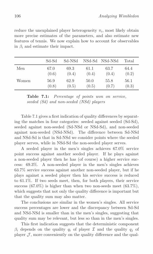
106 Analyzing Wimbledon
reduce the unexplained player heterogeneity πi, most likely obtainmore precise estimates of the parameters, and also estimate newfeatures of tennis. We now explain how to account for observablesin βi and estimate their impact.
Sd-Sd Sd-NSd NSd-Sd NSd-NSd Total
Men 67.0 69.3 61.1 63.7 64.4(0.6) (0.4) (0.4) (0.4) (0.2)
Women 56.9 62.9 50.0 55.8 56.1(0.8) (0.5) (0.5) (0.7) (0.3)
Table 7.1: Percentage of points won on service,seeded (Sd) and non-seeded (NSd) players
Table 7.1 gives a first indication of quality differences by separat-ing the matches in four categories: seeded against seeded (Sd-Sd),seeded against non-seeded (Sd-NSd or NSd-Sd), and non-seededagainst non-seeded (NSd-NSd). The difference between Sd-NSdand NSd-Sd is that in Sd-NSd we consider points where the seededplayer serves, while in NSd-Sd the non-seeded player serves.
A seeded player in the men’s singles achieves 67.0% servicepoint success against another seeded player. If he plays againsta non-seeded player then he has (of course) a higher service suc-cess: 69.3%. A non-seeded player in the men’s singles achieves63.7% service success against another non-seeded player, but if heplays against a seeded player then his service success is reducedto 61.1%. If two seeds meet, then, for both players, their servicesuccess (67.0%) is higher than when two non-seeds meet (63.7%),which suggests that not only the quality difference is important butthat the quality sum may also matter.
The conclusions are similar in the women’s singles. All servicesuccess percentages are lower and the discrepancy between Sd-Sdand NSd-NSd is smaller than in the men’s singles, suggesting thatquality sum may be relevant, but less so than in the men’s singles.
This first indication suggests that the deterministic componentβi depends on the quality qi of player I and the quality qj ofplayer J , more conveniently on the quality difference and the qual-

Quality 107
ity sum, as follows:
βi = β0 + β−(qi − qj) + β+(qi + qj).
In the unlikely event where both new parameters β− and β+ arezero, our model specializes to the model of Chapter 6. Becauseall unobservable determinants are contained in πi, the variablesrelevant to qi are all observable, so qi actually represents observedquality. We don’t know yet what these variables are, so our nextquestion is how to specify qi.
Ranking
Every Monday, with few exceptions, the Association of Tennis Pro-fessionals (ATP, for the men) and the Women’s Tennis Association(WTA, for the women) publish an updated list of the players’ rank-ing points and rankings based on their performance over the pastfifty-two weeks. The method of calculating the ranking points issomewhat complex, but the rankings (1, 2, . . . ) are simply the or-der of the players according to the ranking points. The two lists arealso published just before Wimbledon, and the seedings are based(almost but not entirely) on these lists. We denote the rankings asranki for player I and rankj for player J . The lowest-ranked playerin the tournament may have ranki as high as 500, even though only128 players take part.
A natural first attempt in specifying qi is to equate quality withranking: qi = ranki. In that case, βi and the winning probability piwould depend linearly on the difference between ranki and rankj .This is not satisfactory, because quality in sports is a pyramid: thedifference in strength between numbers 1 and 16 is greater thanbetween 101 and 116.
Hypothesis 10: Quality is a pyramid.
If quality is indeed a pyramid, then going down the pyramidtaking equal steps of quality reduction, the number of players in-volved increases at each step. To see whether this is true we firstconsider the ranking points.
The 2012 end-of-year lists show that Novak Djokovic (12,920points) and Victoria Azarenka (10,595 points) hold the number-one positions at the end of 2012. The same two lists show that

108 Analyzing Wimbledon
there are five players in the men’s singles (three in the women’ssingles) who have between 2000 and 2500 points, seven (thirteen)between 1500 and 2000 points, seventeen (thirty-two) between 1000and 1500 points, and seventy-three (seventy-eight) between 500 and1000 points. So, going down from the top by steps of 500 pointseach, involves more and more players.
This suggests a pyramid, but there are some problems associ-ated with using ranking points as a quality measure. Not only doesthe method of computing ranking points change regularly and differbetween men and women, but more importantly the ranking pointsare artificial creations, not directly related to the players’ true qual-ities. Equal drops in ranking points are therefore not the same asequal steps of quality reduction, and hence we cannot conclude fromthe numerical exercise above that quality is a pyramid. The rank-ings are more robust, and we therefore wish to define quality as afunction of the rankings, not of the ranking points.
Point-winningfreq.,f i
-200 -100 0 100 200 0
20
40
60
80
100
rankj − ranki
-200 -100 0 100 200 0
20
40
60
80
100
rankj − ranki
Figure 7.1: Percentage of winning a point on serviceas a function of the difference in rankings (men left,women right)
Thus motivated, let us use the rankings, rather than the rankingpoints, to study whether quality is really a pyramid. We have dataon fi, so we can plot fi against rankj − ranki. (Remember thata positive value of rankj − ranki means that I is a better playerthan J .) The dots in Figure 7.1 represent the combinations of fi

Quality 109
and rankj − ranki for all matches (two players per match). Thevertical dispersion in the scatter plot is substantial, reflecting thetwo unexplained elements πi (unobserved part of pi) and φi (purenoise).
To summarize the dots in some interpretable curve, we apply astatistical technique called ‘non-parametric’ mean regression. Fora given ranking difference rankj − ranki, say fifty, we take the meanover the fi for which the corresponding rankj−ranki is around fifty.This averages out the unexplained influences on fi to some extent,so that the impact of rankj−ranki on βi and thereby on pi remains.We thus obtain an estimate of this impact, but only for rankj−rankiaround fifty. We now repeat this exercise for many values of theranking difference, and this creates a curve of estimates. This isthe essence of non-parametric mean regression. The technique doesnot impose linearity or any other functional form. The resultingform of the curve is therefore generated by the data and not byunderlying assumptions, and this is useful if we wish to learn aboutthe functional form of the relationship.
The solid curves in Figure 7.1, one for the men and one forthe women, show that pi depends positively on rankj − ranki, asexpected. More important is the shape of the dependence. Appar-ently the relation is non-linear and has the form of an S-curve.
Let us now see how we can use Figure 7.1 to decide whetheror not quality is a pyramid. We first keep ranki constant and varyrankj . We start from rankj − ranki = 0 (the middle of the figure),so that players have equal ranking. When we increase rankj byone, then pi increases and with each further unit increase in rankjthe increase in pi becomes smaller. At about rankj − ranki = 30the curve can no longer be distinguished from a flat curve, so anincrease from 30 to 31 hardly increases pi any more.
Next, we keep rankj constant and vary ranki. A similar flatten-ing occurs. Starting again from rankj−ranki = 0, a unit increase inranki will reduce pi and with each further unit increase in ranki thereduction in pi becomes smaller. Put differently, a given reductionin pi involves larger and larger increments in ranki and thus moreand more players. This is precisely what we mean by a pyramid.So, Figure 7.1 supports hypothesis 10, and we conclude that qual-ity in tennis — and most likely also in other sports — is indeed apyramid.

110 Analyzing Wimbledon
We would like to transform the ranking in such a way that theS-shape is removed, so that βi depends linearly on the transformedranking. We achieve this, based on the idea of a pyramid, by intro-ducing the idea of ‘expected round’: 8 for a player with ranki = 1who is expected to reach the final (round 7) and win, 7 for a playerwith ranki = 2 who is expected to reach the final and lose, 6 forplayers with ranki 3 or 4 who are expected to lose in round 6, 5 forplayers with ranki 5 to 8 who are expected to lose in round 5, andso on. When we walk down the pyramid, more and more playersget the same quality indicator, capturing the flattening of qualitydifferences represented by the idea of a pyramid. A problem withthe expected round, however, is that it does not distinguish be-tween, for example, players ranked 9 to 16, because all of them areexpected to lose in round 4.
Expectedround/8,r
1 100 200 3000.00
0.25
0.50
0.75
1.00
rank
Figure 7.2: Expected round variable r as a functionof the ranking
A smooth measure of expected round is provided by the formula
expected roundi = 8− log2(ranki),
where log2(x) denotes the logarithm of x with base 2. It will beconvenient to scale this formula such that the maximum is 1 ratherthan 8. This then leads to the transformed ranking variable
ri =expected roundi
8= 1− log2(ranki)
8,

Quality 111
which is plotted in Figure 7.2. If ranki = 1 then ri = 1 (the max-imum) reflecting that we expect the world number one to win thetournament. If ranki = 9 then ri = 0.60, and if ranki = 16 thenri = 0.50. The value ri = 0.50 can be interpreted as reaching ‘50%of the tournament’ (round 4 of 8). For players with ranki > 128,we have ri < 1/8, which means that the player was not expected toparticipate in the tournament based on his or her ranking. Play-ers with ranki > 256 will have a negative ri, but this causes noproblems.
Point-winningfreq.,f i
-1 -0.5 0 0.5 1 0
20
40
60
80
100
ri − rj-1 -0.5 0 0.5 1
0
20
40
60
80
100
ri − rj
Figure 7.3: Percentage of winning a point on serviceas a function of the difference in expected rounds (menleft, women right)
Can the (smoothed) expected-round idea explain the S-curvesuggested by the data? To test this we perform another non-parametric mean regression, this time on ri − rj instead of onrankj − ranki. Figure 7.3 shows that the dependence of βi and thuspi on ri−rj is now close to linear. The expected-round transforma-tion implies that constant step-by-step reductions in pi correspondto constant reductions in ri, which involve more and more players.Hence, the transformation fully captures the idea of a pyramid andconverts ranki into units of quality. For example, the quality dif-ference between the numbers 1 (ri = 1) and 16 (ri = 0.5) is twentytimes the quality difference between the numbers 101 (ri = 0.168)and 116 (ri = 0.143).

112 Analyzing Wimbledon
With this knowledge we now specify
qi = ri,
in which case βi can be written as
βi = β0 + β−(ri − rj) + β+(ri + rj).
This would suffice if rankings were the only determinant of pi thatwe can observe and measure. But maybe there is more.
Round, bonus, and malus
Perhaps the performance of a player depends, in addition to theranking of the player and his or her opponent, on the round theyare playing in. A low-ranked player who has managed to progressin the tournament has apparently higher quality than his or herranking indicates, and a top player may not play his or her besttennis in the early rounds. The latter statement in particular isoften heard and therefore worth investigating.
Hypothesis 11: Top players must grow into the tournament.
To analyze both possibilities we distinguish between ‘bonus’,
bonusi = max (roundi/8− ri, 0) ,
and ‘malus’,
malusi = min (roundi/8− ri, 0) .
If roundi/8 > ri, then I has progressed further in the tournamentthan could have been expected on the basis of ranking. There is apositive bonus and no malus. However, if roundi/8 < ri, then I is atop player in an early round, with a negative malus and no bonus.
We specify
qi = ri + αbbonusi + αmmalusi.
For given values of the parameters αb and αm, the quality qi de-pends only on ri and roundi, and Figure 7.4 plots this relationshipfor αb = 0.8 and αm = 0. The figure contains seven partly over-lapping kinked lines, one for each round. Consider a player I who
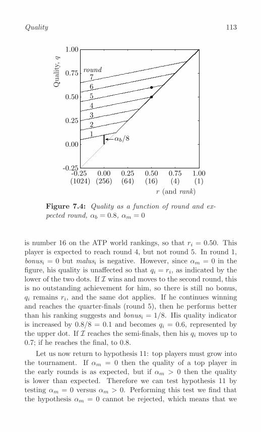
Quality 113
Quality,
q
-0.25 0.00 0.25 0.50 0.75 1.00-0.25
0.00
0.25
0.50
0.75
1.00
round
1
2
3
4
5
6
7
(1024) (256) (64) (16) (4) (1)
8
r (and rank)
Figure 7.4: Quality as a function of round and ex-pected round, αb = 0.8, αm = 0
is number 16 on the ATP world rankings, so that ri = 0.50. Thisplayer is expected to reach round 4, but not round 5. In round 1,bonusi = 0 but malusi is negative. However, since αm = 0 in thefigure, his quality is unaffected so that qi = ri, as indicated by thelower of the two dots. If I wins and moves to the second round, thisis no outstanding achievement for him, so there is still no bonus,qi remains ri, and the same dot applies. If he continues winningand reaches the quarter-finals (round 5), then he performs betterthan his ranking suggests and bonusi = 1/8. His quality indicatoris increased by 0.8/8 = 0.1 and becomes qi = 0.6, represented bythe upper dot. If I reaches the semi-finals, then his qi moves up to0.7; if he reaches the final, to 0.8.
Let us now return to hypothesis 11: top players must grow intothe tournament. If αm = 0 then the quality of a top player inthe early rounds is as expected, but if αm > 0 then the qualityis lower than expected. Therefore we can test hypothesis 11 bytesting αm = 0 versus αm > 0. Performing this test we find thatthe hypothesis αm = 0 cannot be rejected, which means that we

114 Analyzing Wimbledon
have no evidence supporting hypothesis 11. One explanation couldbe that professional tennis is so competitive that top players cannot and do not relax in the early rounds.
We therefore impose αm = 0. But we do not (yet) imposeαb = 0. We estimate αb by αb = 0.7 (0.2) for the men and αb = 0.8(0.2) for the women. The player ranked 16 in the men’s singlesachieves qi = 0.59 when he reaches the quarter-finals, so that heis expected to perform as if he were ranked number 10. A womanplayer ranked 16 achieves qi = 0.60 when she reaches the quarter-finals, and is expected to be of the same quality as the world’snumber 9.
Significance, relevance, and sensitivity
We set αm = 0, because its estimate is not significantly differentfrom zero. We now also set αb = 0, in spite of the fact that itsestimate is significant. With both αm and αb equal to zero, thequality qi depends only on the rank: qi = ri.
Surely, this is a bit strange. The estimate of αb is significantlydifferent from zero, and still we set the parameter equal to zero.How can we justify such a modeling decision? For this we need tounderstand the difference between significance and relevance.
Suppose we consider a model where the variable to be explained,say h, depends on u and a number of other variables:
h = θu+ other things.
We don’t know the value of the parameter θ, which we assumenot to be zero, but we can estimate it when appropriate data areavailable. The more (and better) data we have, the more accuratelywe can estimate θ, and the smaller will its standard error be. Whenthe standard error is very small, then the hypothesis that θ = 0 willalmost certainly be rejected. Put differently, the estimate θ will be‘significant’, as explained on page 77.
It is perfectly possible, however, that the impact of θu on h issmall compared to the impact of the other variables in the model,even though θ is significant. The variable u is then not ‘relevant’.We want to avoid variables that are not relevant, because estimat-ing the associated parameters adds uncertainty and this makes thestandard errors of the other estimates larger, which is undesirable.

Quality 115
What we really want to know is not so much whether the esti-mate of a parameter is significant or not, but whether the answer tothe question under investigation changes when we set the parame-ter equal to zero. If the answer changes, then our research questionis sensitive to this parameter; if not, it is not sensitive.
Significance and sensitivity are two different concepts, and theyare essentially unrelated. Knowledge of one tells you very littleabout the other. A parameter estimate may be significant but theanswer to our research question may not be sensitive to setting theparameter equal to zero, and vice versa.
In our case, the estimate of αm is not significant, while the esti-mate of αb is significant. Neither parameter is sufficiently relevant.Therefore we set both parameters equal to zero and include neithermalus nor bonus in our model.
The complete model
This completes our model. Let us briefly summarize it. The relativefrequency fi and the probability pi are related through noise φi:
fi = pi + φi.
The relative frequency can be observed from the data, but the prob-ability cannot be observed and needs to be modeled. We assumethat it depends on deterministic components βi and random com-ponents πi:
pi = βi + πi,
where we have specified βi as
βi = β0 + β−(ri − rj) + β+(ri + rj).
Combining terms we find
fi = β0 + β−(ri − rj) + β+(ri + rj) + πi + φi.
From now on we shall usually write ‘ranking’ when we mean ‘trans-formed ranking’, unless there is a possibility of confusion.

116 Analyzing Wimbledon
For each match the average of the two ranking differences is zero,so the average ri − rj in the sample is also zero. We subtract theaverage ranking sum from ri + rj (‘centering’), so that the rankingsum also has mean zero. This gives βi = β0 for the average match,so that β0 keeps its interpretation as the overall average probability.The centering is only introduced for convenience of interpretation;it does not affect the results.
The error term is πi+φi, and we need assumptions on its behav-ior in order to derive moment conditions for estimation, as in theprevious chapter. The error term still has zero expectation, so thatthe original moment condition E(fi) = βi still applies. In contrastto the previous chapter, however, we now have three parameters inβi, namely β0, β−, and β+, instead of just β0, and we cannot solveall three parameters from a single moment condition. Fortunately,the ranking variables ri and rj are uncorrelated with the error, andthis yields two additional moment conditions:
E ((fi − βi)(ri − rj)) = 0, E ((fi − βi)(ri + rj)) = 0.
Under suitable assumptions, discussed in the previous chapter, wethen arrive at the five moment conditions,
E(fi − βi) = 0,
E ((fi − βi)(ri − rj)) = 0,
E ((fi − βi)(ri + rj)) = 0,
var(fi) = σ2 + E
(fi(1− fi)
Ti − 1
),
cov(fi, fj) = ρσ2.
These five conditions allow us to estimate the unknown parametersβ0, β−, β+, σ, and ρ and compute their standard errors.
Winning a point on service
We first present the estimation results for pi, the probability of win-ning a point on service. In the first and third rows of Table 7.2 weestimate the restricted model where β− = β+ = 0, so that qualityβi = β0 is constant for all players. This is the model estimated inChapter 6, and the estimates (64.4% for the men and 55.9% for the

Quality 117
women) correspond to the estimates presented in Table 6.1, columnGMM. The estimates of the heterogeneity parameter σ and the cor-relation parameter ρ also agree with the estimates in Chapter 6.
β0 β− β+ σ ρmean ri − rj ri + rj heterog. correl.
MenNot using ranking 64.4 − − 5.9∗ −0.51∗
Using ranking 64.9 8.0∗ 3.1∗ 5.0∗ −0.44∗
WomenNot using ranking 55.9 − − 6.7∗ −0.92∗
Using ranking 56.3 15.9∗ 1.8◦ 4.2∗ −0.79∗
Table 7.2: Explaining the probability of winning apoint on service
In the second and fourth rows we estimate the complete model.Taking quality into account hardly affects the estimates of β0, whichis consistent with the fact that β0 still reflects the overall averageprobability of winning a point. The effect of quality difference (ri−rj) on pi is much larger than the effect of quality sum (ri + rj), asexpected.
Hypothesis 12: Men’s tennis is more competitive than women’stennis.
This issue was addressed in Chapter 2, where we concludedthat there are more upsets (top-sixteen seeds not reaching the lastsixteen) for the men than for the women, in line with the hypothesis.Table 7.2 provides new evidence based on two improvements: wework at point level rather than at match level, so that the analysisnow takes account of the difference between best-of-five versus best-of-three matches; and we use rankings, which is a better indicatorof quality than the earlier distinction between seeds and non-seeds.
The estimated β− is smaller for the men (8.0) than for thewomen (15.9), and significantly so. Apparently, the ranking is moreinformative for women than for men, which means that the differ-ence in strength between top and lower-ranked players is greater

118 Analyzing Wimbledon
in the women’s singles than in the men’s singles, again supportinghypothesis 12.
We notice the possibility of confusion in the terms ‘lower rank’and ‘higher rank’. The best player has world ranking 1, but incommon language (and also in tennis terminology) such a playerhas a high rather than a low ranking. We follow common languageand emphasize that here and in the following a lower-ranked playeris a player with a lower ri-value than a higher-ranked player, thatis, a player of lower quality.
Point-winningprob.,pi
b
0
b
-1 -0.5 0 0.5 1 0
20
40
60
80
100
ri − rj
b
0
b
-1 -0.5 0 0.5 1 0
20
40
60
80
100
ri − rj
Figure 7.5: Probability of winning a point on serviceas a function of expected-round difference (men left,women right)
We plot the dependence of pi on quality difference in Figure 7.5for a player having zero unobserved quality πi, keeping quality sumat its average value. At the figure’s extreme we have ri−rj = 1 and
hence the probability of winning a point for the men is β0 + β− =72.9% for player I and β0 − β− = 56.9% for player J . For thewomen, the probability of winning a point is β0 + β− = 72.2% forplayer I and β0 − β− = 40.4% for player J . The shadow aroundthe estimated line represents estimation uncertainty, implied by thestandard errors of the estimated parameters. The estimation uncer-tainty turns out to be small, much smaller than the heterogeneity σ.

Quality 119
Table 7.2 also shows that there is more unobserved heterogeneity(σ = 5.0) for the men than for the women (σ = 4.2), which is coun-terintuitive and therefore worth noting. It is counterintuitive be-cause the men’s game is more competitive than the women’s game,and one would therefore expect less rather than more heterogeneity(more rather than less homogeneity). Indeed, when we ignore thequality effect, we do find less heterogeneity (σ = 5.9) for the menthan for the women (σ = 6.7), as shown in Table 7.2. Accountingfor ranking in the model makes part of the heterogeneity observ-able, so that the remaining unobserved part σ is reduced. Thisapplies to both men and women. But because β− is much largerfor the women than for the men, the reduction in σ is larger for thewomen, and this more than offsets the initial excess heterogeneityfor the women.
Including quality in our model makes the deterministic partmore complete and the random part less important. We see thisreflected in the results, because both σ and ρ become smaller (closerto zero) when quality is included. The model explains more and istherefore better than the model of the previous chapter.
Other service characteristics
We perform the same analysis on other service characteristics, andthe results are presented in Table 7.3. The table confirms the con-clusions from Table 7.2: the estimated β0 is not much affected whenquality is included; ranking difference matters more than rankingsum; and heterogeneity is reduced by including quality.
The more complete analysis does, however, change the conclu-sion regarding hypothesis 6, which states that the probability thatthe service is in is the same in the men’s singles as in the women’ssingles. The estimated probability of first service in for the averagematch is β0 = 59.6% with a standard error of 0.3% for the men, and61.6% (0.5%) for the women. The difference is 2.0 (0.6), which issignificant, while the earlier analysis (page 92) based on the modelwithout rankings led to an insignificant difference. The reason isthat the estimate for the women has slightly changed and that thestandard errors have become smaller, because the inclusion of rank-ings has lowered the unexplained part. For the second service theprobabilities for the average men and women remain remarkably

120 Analyzing Wimbledon
β0 β− β+ σ ρmean ri − rj ri + rj heterog. correl.
Men1st service (s.) in 59.6 −0.1◦ 0.8◦ 5.0∗ −0.03◦
2nd service in 86.5 1.5∗ 0.7◦ 3.3◦ 0.11◦
Points won if 1st s. in 74.0 8.1∗ 4.0∗ 5.9∗ −0.08◦
Points won if 2nd s. in 59.6 8.2∗ 1.3◦ 5.3∗ −0.41◦
Points won on 1st s. 44.1 4.7∗ 2.9∗ 4.9∗ −0.36∗
Points won on 2nd s. 51.6 8.0∗ 1.5◦ 5.2∗ −0.54∗
Women1st service in 61.6 0.3◦ 4.3∗ 6.8∗ 0.03◦
2nd service in 86.7 4.6∗ 4.5∗ 4.8∗ −0.16◦
Points won if 1st s. in 62.9 16.8∗ 1.4◦ 5.0∗ −0.51◦
Points won if 2nd s. in 52.8 13.5∗ −2.4◦ 7.7∗ −0.49◦
Points won on 1st s. 38.7 10.6∗ 3.7∗ 3.6∗ −0.88∗
Points won on 2nd s. 45.8 14.1∗ 0.4◦ 7.2∗ −0.48◦
Table 7.3: Service probabilities explained
close. Our final conclusion is that hypothesis 6 is rejected for thefirst service, but not for the second.
The separation of pi into its building blocks provides further in-sights. We first examine the β− estimates. The reason (or at leastone reason) why better players win more points is not that theyhit more first services in (the estimates −0.1 and 0.3 are insignif-icant), but that they hit more second services in (1.5 and 4.6 aresignificant). Maybe players with a better ranking than their op-ponents go for a safer second service, assuming that they will winthe resulting rally anyway. We cannot test this directly, becausewe do not observe what would have happened if a player had usedhis or her usual second service. However, our claim is somewhatsupported by comparing the probability of points won if the secondservice is in to the probability of points won if the first service isin. The latter probability is 8.1 (men) and 16.8 (women) higherfor the better server. The increments for the second service (8.2and 13.5) are not significantly lower. Better players can thereforeafford to play a safer second service. This does not mean that it is
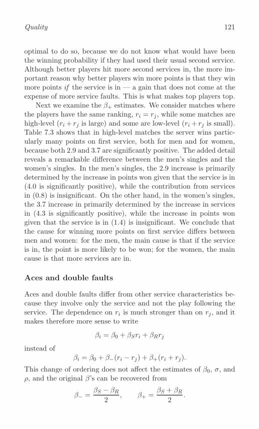
Quality 121
optimal to do so, because we do not know what would have beenthe winning probability if they had used their usual second service.Although better players hit more second services in, the more im-portant reason why better players win more points is that they winmore points if the service is in — a gain that does not come at theexpense of more service faults. This is what makes top players top.
Next we examine the β+ estimates. We consider matches wherethe players have the same ranking, ri = rj , while some matches arehigh-level (ri+ rj is large) and some are low-level (ri+ rj is small).Table 7.3 shows that in high-level matches the server wins partic-ularly many points on first service, both for men and for women,because both 2.9 and 3.7 are significantly positive. The added detailreveals a remarkable difference between the men’s singles and thewomen’s singles. In the men’s singles, the 2.9 increase is primarilydetermined by the increase in points won given that the service is in(4.0 is significantly positive), while the contribution from servicesin (0.8) is insignificant. On the other hand, in the women’s singles,the 3.7 increase in primarily determined by the increase in servicesin (4.3 is significantly positive), while the increase in points wongiven that the service is in (1.4) is insignificant. We conclude thatthe cause for winning more points on first service differs betweenmen and women: for the men, the main cause is that if the serviceis in, the point is more likely to be won; for the women, the maincause is that more services are in.
Aces and double faults
Aces and double faults differ from other service characteristics be-cause they involve only the service and not the play following theservice. The dependence on ri is much stronger than on rj, and itmakes therefore more sense to write
βi = β0 + βSri + βRrj
instead ofβi = β0 + β−(ri − rj) + β+(ri + rj).
This change of ordering does not affect the estimates of β0, σ, andρ, and the original β’s can be recovered from
β− =βS − βR
2, β+ =
βS + βR2
.

122 Analyzing Wimbledon
The sign of βS in Table 7.4 shows, not unexpectedly, that betterplayers serve more aces (especially in the men’s singles) and fewerdouble faults (especially in the women’s singles). The sign of βRshows that the better is the receiver, the fewer aces are served inthe women’s singles. However, there is no evidence that the qualityof the receiver influences the number of double faults (for eithermen or women) or the number of aces for the men.
β0 βS βR σ ρmean ri rj heterog. correl.
MenAces 8.8 6.8∗ 0.8◦ 5.0∗ −0.16∗
Double faults 5.5 −1.0∗ 0.2◦ 1.8∗ −0.08◦
WomenAces 3.2 3.0∗ −3.1∗ 1.8∗ −0.66∗
Double faults 5.1 −4.0∗ −0.5◦ 2.3∗ −0.03◦
Table 7.4: Ace and double fault probabilitiesexplained
We return briefly to hypothesis 7 by testing whether the percent-age of double faults is the same for men and women. The estimatesfor the average player are 5.45 (0.15) for the men and 5.10 (0.22) forthe women. The difference is 0.35 and has a standard error of 0.27,leading to a confidence interval (−0.18, 0.88). The interval coverszero, just as the intervals on pages 80 and 92 where we tested thesame hypothesis using simpler tools. The hypothesis is thereforenot rejected, at least for the average player.
How do we reconcile this with the results from the previous sec-tion, in particular the fact that the probability of first service inis not the same for men and women, but the probability of secondservice in may be the same? The answer is estimation uncertainty.If one combines two differences, one of which is significant and onewhich isn’t, then it may well happen that the difference of thecombination (double fault) has a large standard error, so that itbecomes insignificant. Our final conclusion regarding hypothesis 7is therefore that we do not reject it (on average). It remains re-

Quality 123
markable that the double fault probabilities are so close betweenmen and women, given the differences between men’s and women’stennis.
Further reading
Until 1967 only amateurs could compete at grand slam tourna-ments, but from 1968 onwards professionals could compete as well,and the ‘open’ era in tennis was born. In 1972 the leading profes-sionals created the ATP, and one of their first acts was the establish-ment of a ranking system. The ATP Rankings began on August 23,1973 and has continued to be the official ranking system in men’sprofessional tennis until today. In 1973 Billie Jean King foundedthe WTA. The WTA Rankings started on November 3, 1975. Bothranking systems are published weekly. For a comparison of theATP and WTA ranking systems to systems used in other sports,see Stefani (1997).
Although these two systems dominate tennis rankings, alterna-tive systems have been proposed. Blackman and Casey (1980), forexample, introduced a rating method for all serious tennis players— professionals and amateurs — that can be applied to define atennis handicap, so that players with different skills can competeon even terms, just as in golf. Our book only uses the ATP andWTA rankings. We do not, however, use the rankings directly,but transform them using the expected-round concept (page 110),introduced in Klaassen and Magnus (2001).
The literature has tested whether variables other than rank-ings are relevant to tennis-winning probabilities. The overall con-clusion is that the ranking difference is by far the most impor-tant determinant, and this conclusion is confirmed by our analysis.We briefly review this literature. Del Corral and Prieto-Rodrıguez(2010) study the determinants of match wins at the grand slamtournaments 2005–2008. The most important determinant is theranking, more precisely the difference in logarithmic rankings (fol-lowing our expected-round concept). They also include other pos-sible determinants, such as age, height difference, round, and right-and left-handedness. These do not appear to have much impact,except age: for the higher-ranked player the probability of winningthe match is lower if he or she is older than the opponent.

124 Analyzing Wimbledon
The fact that Del Corral and Prieto-Rodrıguez do not find aleft-handedness effect, is somewhat contrary to common opinion,which is that ‘lefties’ have an advantage. Holtzen (2000) reportsthat about 10% of the general population is left-handed, and ofprofessional tennis players also about 10%. But in the group oftop players lefties are seriously overrepresented. Rod Laver, JimmyConnors, John McEnroe, Rafael Nadal, Martina Navratilova, andMonica Seles are all left-handed, and over the period 1968–1999 left-handed players held the number-one ranking position about 35%of the time, both for men and for women. Roger Federer offeredthe explanation that left-handers typically get breakpoints on theirfavorite side, so that their swinging serves provide an advantage,especially when the receiver has a one-handed backhand. In termsof Chapter 4, we know that the average importance of points servedin the ad court is higher, and this is precisely the side where leftiescan serve out wide.
If left-handedness provides an advantage, this does not implythat in explaining or predicting point- or match-winning probabil-ities we need to take left-handedness into account if we include therankings in our analysis. Any advantage for left-handed playerswill occur in every match, so that it will show up in the rankings.Therefore, if we correct for ranking, left-handedness does not mat-ter much any longer. The suitability of this indirect way of dealingwith left-handedness is confirmed by the results of Del Corral andPrieto-Rodrıguez (2010). In addition, our unobserved quality cor-rection π accounts for any remaining effect of left-handedness, as itdoes for any variable that is constant throughout the match.
A final potential determinant of quality is home advantage. Al-though less important than in team sports (such as football), homeadvantage may also exist in individual sports (such as tennis). Ten-nis players may be affected by crowd support and familiarity withlocal circumstances. Holder and Nevill (1997) find little evidence,but Koning (2011) finds an advantage, significant for men, insignif-icant for women. Whatever the truth, our unobserved quality cor-rection π properly accounts for home advantage, because it remainsconstant throughout the match.
The test of hypothesis 12 on the competitiveness of men’s ver-sus women’s tennis is used in Klaassen and Magnus (2001). Koning(2009) applies the test to more recent data (through 2008) and

Quality 125
shows that competition in men’s tennis is still tougher than inwomen’s tennis. The results by Del Corral (2009) over 1994–2008confirm this. These are relative results: men compared to women.Rohm et al. (2004) show that competitiveness in the men’s singlesat Wimbledon 1968–2001 has been high also in an absolute sense.

This page intentionally left blank

8First and second service
Two services are allowed in tennis. This is an unusual feature com-pared to other sports with a service (table tennis, badminton, vol-leyball), and it allows intriguing questions — for example, whethera player is as good as his or her second service, as is often heard.Also, having two services offers a challenge for tennis players andinvestigators to think about the optimal balance between the twoservices. From a data point of view, it doubles the amount of in-formation per player, allowing more precise analyses.
The optimal balance between the two serves requires a theoret-ical framework, which will be introduced in the next chapter. Thecurrent chapter offers a deeper analysis of the first and second ser-vice winning probabilities, and explains why we should move froman analysis of each service characteristic individually to a frame-work in which we examine the two characteristics jointly.
Is the second service more important than the first?
For some of the hypotheses considered so far it sufficed to use overallaverages only. One hypothesis where this cannot be done is thefollowing.
Hypothesis 13: A player is as good as his or her second service.
Overall averages are not useful here, because quality matters,so that we have to differentiate between players. We have to definewhen a player is ‘good’ and also when a second service is ‘good’.
A service is ‘good’, as argued on page 75, when the percentageof points won on that service (not the percentage of services in or

128 Analyzing Wimbledon
the percentage of points won if the service is in) is high. When aplayer is ‘good’ is less easy. We offer three interpretations.
Absolute quality
One possibility is to say that a player is ‘good’ if he or she is seeded.A player is then good compared to the group of players in the tour-nament as a whole without considering the opponent in the cur-rent match. For example, Serena Williams is good, irrespective ofwhether her opponent is Maria Sharapova or the world number 100.We call this absolute quality.
When a seed serves in the men’s singles, taking seeded and non-seeded receivers together, the probability of winning a point on firstservice is 46.3%, while the probability on second service is 55.1%,a difference of 8.8%-points. The estimates are simply the relativefrequencies in the data. When a non-seed serves, the percentagesare 42.7% and 50.2%, a difference of 7.5%-points. Apparently, aseed in the men’s singles wins particularly many points on his sec-ond service, in line with the hypothesis. But for the women thedifferences are 8.4% and 8.9% for a seed and non-seed, respectively.Hence, contrary to the hypothesis, a seed in the women’s singlesdoes not win especially many points on her second service.
Absolute quality corrected for quality difference
The previous interpretation distinguishes between the quality ofservers, but not of receivers. This has the consequence that if weconsider a non-seeded instead of a seeded server, then two thingshappen: we lower the quality of the server and also the qualitydifference between server and receiver. Perhaps these two changeshave opposite effects, and combining them causes the above am-biguous result for men and women.
To find out, we now distinguish also between seeded and non-seeded receivers. Table 8.1 is the same as Table 7.1, except thatwe have separated the first and second service. We first compareSd-Sd and NSd-NSd matches. With some simplification one maythink of the players in such matches as being of the same strength:either both seeded or both non-seeded. So when comparing seedsto non-seeds, the quality difference is not affected. This is the

First and second service 129
Sd-Sd Sd-NSd NSd-Sd NSd-NSd
MenPoints won on 1st service 45.6 46.5 41.7 43.0Points won on 2nd service 51.8 56.3 47.6 51.0
WomenPoints won on 1st service 41.0 42.8 34.1 37.1Points won on 2nd service 46.0 52.2 40.4 47.0
Table 8.1: Percentage of points won on first and sec-ond service, seeded (Sd) and non-seeded (NSd) players
absolute point of view, but now corrected for the impact of qualitydifferences.
In the men’s singles, seeded players win many more points ontheir first service than non-seeded players (45.6% > 43.0%). Thefact that seeds win more points is not as obvious as it may seem atfirst, because not only the service but also the opponent’s returnof service will be better. For the second service, the probabilityof winning a point differs much less (51.8% versus 51.0%). Thesituation is similar in the women’s singles. There is a 3.9%-pointdifference between seeded and non-seeded players on the first ser-vice, and only −1.0%-point on the second service. It seems thereforethat hypothesis 13 is not supported by the data. If anything, thehypothesis ‘a player is as good as his or her first service’ would bemore appropriate.
Relative quality
In the previous analysis we compared Sd-Sd to NSd-NSd, so thatthere is variation in the overall quality of the match, but the qual-ity difference is kept constant. We can also keep the overall qual-ity constant and vary the quality difference. This is achieved bycomparing Sd-NSd to NSd-Sd: the relative interpretation. In themen’s singles, Table 8.1 shows that a seeded player wins 46.5% ofpoints on his first service against a non-seed, while a non-seededplayer wins 41.7% of his points on first service against a seed, adifference of 4.8%-points. On the second service the difference is

130 Analyzing Wimbledon
larger: 56.3 − 47.6 = 8.7%-points. In the women’s singles, the dif-ference on the second service is also larger than on the first service(11.8 > 8.7). These comparisons suggest that the performance onthe second service tells us more about a player’s quality than thefirst.
We now have three interpretations and mixed outcomes. Allthree interpretations make sense. So is hypothesis 13 false or not?
Differences in service probabilities explained
To make further progress we reconsider Table 7.3, based on themodel of pages 115 and 116.
β0 β− β+mean ri − rj ri + rj
MenPoints won on 1st service 44.1 4.7∗ 2.9∗
Points won on 2nd service 51.6 8.0∗ 1.5◦
Difference −3.3∗ 1.4◦
WomenPoints won on 1st service 38.7 10.6∗ 3.7∗
Points won on 2nd service 45.8 14.1∗ 0.4◦
Difference −3.5◦ 3.3◦
Table 8.2: Difference between first and second servicewinning probabilities explained
Table 8.2 contains the numbers from this table that are rele-vant to our investigation. The impact of ri on each of the twoservice-winning probabilities depends on two variables: the qualitydifference (ri − rj) and the quality sum (ri + rj). Adding β− andβ+ thus provides the impact of ri when rj is kept constant. This isthe absolute effect. If we leave out the impact via ri− rj, we obtainthe absolute effect corrected for quality difference, represented byβ+. Finally, β− captures the relative effect. We discuss the resultsof all three interpretations in turn.

First and second service 131
Regarding the absolute interpretation, we compute the sumsof β− and β+. All four sums are positive, as expected, becausehigher-ranked servers (that is, servers with a higher ri-value) scoremore points on first and on second service. The question is onwhich service they are particularly successful. For the men thedifference between the first and second service sums is 1.9, and forthe women 0.2, both in favor of the second service. These differencesare, however, not significant, so there is no clear evidence in favorof hypothesis 13.
The second interpretation is obtained by filtering out the qual-ity difference impact, thus focussing on the estimates of β+. In themen’s singles we find 2.9 > 1.5, so that the higher the quality ofthe match the more points are won on first service compared to sec-ond service. The performance on first service tells us more aboutquality than the second service, contradicting hypothesis 13. Thewomen’s singles lead to the same conclusion: 3.7 > 0.4. This is thesame outcome as in the analysis based on seeds and non-seeds, butwe have not yet examined the significance of these results. In theearlier analysis, based on seeds and non-seeds, the seeds performsignificantly better on first service, while the performances on sec-ond service do not differ significantly. This is true for both men andwomen. In the current model-based analysis, the outperformanceon first service is 1.4 for the men and 3.3 for the women, neitherof which is significant. The reason why we get different results isthat the standard errors computed in the first analysis are too small(see also page 91). Again we see the importance of proper statisti-cal modeling for inference. We conclude that there is no compellingevidence against hypothesis 13 from the (corrected) absolute pointof view.
Finally, we consider the relative approach by looking at β−,which reflects the impact of the quality difference ri− rj . Table 8.2shows that 4.7 < 8.0 in the men’s singles, so that the better theserver relative to the receiver, the more points he wins on the secondcompared to first service. The second service performance now saysmore about his quality than the first service performance, in linewith hypothesis 13. This is confirmed in the women’s singles, andit is the same result as in the seeded versus non-seeded analysis.The difference of −3.3 for the men is significant, but the difference−3.5 for the women is not.

132 Analyzing Wimbledon
What have we learned from these three interpretations? Thatthere is no compelling evidence against hypothesis 13, nor in theabsolute sense (corrected or not), nor in the relative sense. In fact,there is some evidence in favor of the hypothesis in the relativeinterpretation. Hence we conclude that a player is as good as hisor her second service, as the hypothesis states.
If it is true that players distinguish themselves more with thesecond service than with the first, then this has consequences forthe possible change-of-rule discussed on page 28, namely to allowonly one service. If only one service were allowed rather than two,then not only would the probability of winning a point on servicedecrease for all players, but also the difference between good andless good players would become larger. This is so, because the topplayers apparently distinguish themselves by their second service,and this is precisely the service that would remain after the rulechange.
Joint analysis: bivariate GMM
One may object that our method of computing the standard errorof the difference between the first- and second-service estimatorsis not entirely correct. In general, the variance of the differencebetween two estimators, say θ1 and θ2, is equal to the sum of theindividual variances minus twice the covariance between the twoestimators:
var(θ1 − θ2) = var(θ1) + var(θ2)− 2 cov(θ1, θ2).
What we have done in the previous calculations is set the covarianceequal to zero. However, the covariance will not be zero in general,because the first and second services are correlated — the betterplayer will not only score more points on the first service, but alsoon the second service. The estimates themselves are not incorrect,but if we wish to compare them, then we need an estimate of thecovariance. How can we generalize our ‘complete’ model, presentedon pages 115 and 116, to include the covariance?
One source of correlation between the probabilities of winninga point on first and second service is related to the world rankingsof the players. If the server has a top ranking, then both the prob-ability of winning a point on first and on second service will be

First and second service 133
high, causing a correlation. Because we include the same rankingvariables ri − rj and ri + rj in the models of both probabilities,this part of the correlation is observed and is accounted for in theestimation results so far.
The other source of correlation comes from πi, the part of theprobability that we do not observe. The form of the day, for ex-ample, affects the winning probabilities on both services, leading tocorrelation between the two probabilities. This correlation is notaccounted for when the equations are estimated for each serviceprobability separately, as we have done so far.
To properly account for the second source of correlation we com-bine the models for the first and second service-winning probabili-ties, allowing the two πi-variables to be correlated. In other words,what we try to explain is no longer two separate probabilities, butrather a pair of two. Instead of our one-dimensional (univariate)GMM procedure we need a two-dimensional (bivariate) procedure— a little more complicated. Joint estimation (estimation of thebivariate model) automatically yields an estimate of the covariancebetween the estimators of the two β-parameters. An additionalbenefit is that joint estimation takes full advantage of the informa-tion that the data on the first service provide on the second serviceparameters and vice versa. This generally leads to smaller standarderrors.
The estimates resulting from joint estimation are the same asthe estimates in Table 8.2. This is not surprising because the mo-ment conditions are the same. The additional estimates concernthe correlation between the two πi-variables. In the men’s singleswe find a correlation between first and second service probabilityof 0.52; in the women’s singles it is 0.27, both positive, in line withour expectation.
Our main interest, however, is in another correlation, namelybetween the first- and second-service estimators of β− and β+. Forβ− the correlation is 0.22 for the men and −0.07 for the women.For β+ the correlations are 0.14 and 0.20, respectively. All fourcorrelations are small (close to zero), which suggests that settingthe covariance equal to zero, as we did in the previous section, maybe the right thing to do. All results in Table 8.2 remain valid, andour conclusion at the end of the previous section, that a player isas good as his or her second service, remains valid as well.

134 Analyzing Wimbledon
Four service dimensions
In Table 8.1 we presented a breakdown of the probability p of win-ning a point on service in two components, one for the first and onefor the second service. The probability of winning a point on thefirst service is itself made up of two components: the probabilitythat the first service is in and the probability of winning the pointif the first service is in. The same is true for the second service.In Table 8.3 we present this further breakdown, resulting in fourdimensions.
Sd-Sd Sd-NSd NSd-Sd NSd-NSd
Men1st service in 58.7 59.5 59.4 59.52nd service in 87.8 87.3 85.6 86.2Points won if 1st service in 77.7 78.1 70.2 72.4Points won if 2nd service in 59.0 64.5 55.6 59.2
Women1st service in 65.6 61.5 60.5 60.22nd service in 88.8 89.1 85.2 85.0Points won if 1st service in 62.5 69.6 56.4 61.7Points won if 2nd service in 51.8 58.6 47.4 55.2
Table 8.3: Four service dimensions, seeded (Sd) andnon-seeded (NSd) players
The percentages are in line with our earlier conclusions. Becauseof the problems that the corresponding standard errors may causefor inference, we immediately move to our model-based approach.
Four-variate GMM
One collection of model-based estimates of the four probabilitieswas presented in Table 7.3. These estimates were obtained for eachprobability separately. We know from the bivariate GMM sectionthat estimating probabilities jointly improves the estimation resultsby exploiting the correlations between the πi-variables. The four

First and second service 135
service characteristics considered here will, in general, be correlated.In particular, the correlation between the probabilities of winningthe point if the first or second service is in will be positive, becausebeing in a good form (that is, performing better than the rankingsuggests, πi > 0) will increase both winning probabilities. Thesame applies to the service-in probabilities: if a player hits morefirst services in, then very likely he or she will also hit more secondservices in.
We exploit information from the data on such correlations byestimating the four probabilities jointly, which results in a four-dimensional (four-variate) GMM procedure. This will be the mostadvanced model in this book. We shall need its estimates in the nextchapter, but we can already use the model here to our advantage.
β0 β− β+mean ri − rj ri + rj
Men1st service in 59.5 0.1◦ 0.6◦
2nd service in 86.4 1.6∗ 0.7◦
Points won if 1st service in 74.0 8.4∗ 3.4∗
Points won if 2nd service in 59.4 7.9∗ 0.9◦
Women1st service in 61.6 0.6◦ 3.9∗
2nd service in 86.4 4.4∗ 4.3∗
Points won if 1st service in 63.1 17.0∗ 1.2◦
Points won if 2nd service in 52.6 13.8∗ −2.2◦
Table 8.4: Four service dimensions explained in afour-variate analysis
Table 8.4 presents a subset of the estimation results, namely theestimated value and significance of β− (the impact of the qualitydifference ri−rj) and the estimated value and significance of β+ (theimpact of the quality sum ri+rj). The estimates of the correlationsare in line with what we expect, and we do not present them.
The estimates in Table 8.4 are almost the same as those obtainedfrom estimating the four characteristics one by one, as reported in

136 Analyzing Wimbledon
Table 7.3. This is good news and corroborates our findings basedon the bivariate model. The conclusions drawn in earlier chapterstherefore still apply. For example, as concluded from Table 7.3, if Iis the better player in a match (ri > rj), then he or she wins morepoints not because I hits more first services in, a little because Ihits more second services in, but mostly because I performs well ifthe service (first or second) is in.
Further reading
Hypothesis 13 has been analyzed earlier in Magnus and Klaassen(1999b).

9Service strategy
Both players in a tennis match attempt to maximize the probabilityof winning the match. If points are independent, then each serverchooses the service strategy that maximizes the probability of win-ning a point. A good strategy involves making both services neithertoo easy (in which case the receiver will kill it) nor too difficult (inwhich case the service will too often be a fault). We develop amodel to answer the question of how difficult a player should makehis or her service in order to maximize the probability of winning apoint on service. We then test how close tennis professionals are tothis maximum, that is, how efficient their service strategy is. Wealso ask whether top players are more efficient servers than other,lower-ranked, tennis professionals.
The server’s trade-off
As always, we consider a match between I and J . Player I servesand has to decide what type of first service to use and, if the firstservice is a fault, what type of second service. If I decides to go fora flat fast first service down the middle, and if the service happensto be in, then the probability of winning the point is high. Butthe probability that this service is in is low. If, on the other hand,I decides to go for an easy service, then the probability that theservice is in is high, but the probability of winning the point if theservice is in is low.
Hence there is a trade-off, and it is not clear what the overalleffect of going for the easier service will be. This is already difficultif I had only one service at his or her disposal, and it becomes

138 Analyzing Wimbledon
even more difficult with two services. The key probabilities in thetrade-off are the probabilities introduced in the previous chapter.We denote them by
x1: probability that first service is in,x2: probability that second service is in,y1: probability of winning the point if first service is in,y2: probability of winning the point if second service is in.
The probability p of winning a service point can then be computedas
p = x1y1 + (1− x1)x2y2,
in accordance with the discussion on page 75. Here we see theformalization of the trade-off. Increasing x2 has the direct effect ofincreasing p, and also the indirect effect of lowering y2 and hencedecreasing p. This is the trade-off for the second service. Thesame applies to the first service, but here there is an additionaleffect, because increasing x1 leads to a lower value of 1 − x1, thusreducing the possible contribution of the second service to winningthe point. The question in this chapter is how to determine theplayer’s optimal service strategy (x1, x2).
The question can easily become too complicated to answer.Thus we impose restrictions to keep the problem manageable, inaccordance with Albert Einstein’s words: simple but not too sim-ple. One assumption that we already imposed is that players serveto maximize the probability of winning. This seems a reasonableassumption, especially for professional players. Amateur players,however, may have a slightly different objective. Casual observa-tion suggests that amateurs often fully attack the first serve, mak-ing the service more difficult than their skills allow, so that the firstservice is frequently out or in the net. But the satisfaction fromserving the odd ace makes up for this inefficient service behavior.Amateurs typically also make their second service too easy, so as toavoid the disappointment of a double fault. For amateurs, satisfac-tion may be more important than winning. It is unlikely, however,that professionals behave this way. They want to win.
Another restriction is that we confine the analysis to the four keyprobabilities x1, x2, y1, and y2. We realize that, for both services,x and y depend on several variables, such as speed, direction, spin,

Service strategy 139
concentration, emotions, and so on. Since we have no data on theseadditional variables, we assume that the variables that matter forx are chosen optimally given the value of x. Since we study theworld’s best tennis players this assumption seems reasonable, andit allows us to act as if only x matters for y and hence for p, so thatthe server has to choose only x1 and x2.
The y-curve
We shall develop a mathematical model for the server. A key ele-ment in this model is a function y(x) relating the probability x thatthe service is in to the probability y that I wins the point if theservice is in. There are two services but there is only one y-curve(per player, because each player may have a different curve). Thetwo services represent different points on that curve: y1 = y(x1)and y2 = y(x2) for the first and second services, respectively.
Point-winningprob.,y
0 20 40 60 80 100 0
20
40
60
80
100
( 1 1)
( 2 2)
Service-in prob., x
Figure 9.1: The y-curve
To illustrate, consider the estimated probabilities for an averagematch in the men’s singles, as reported in Table 8.4. We find
(x1, y1) = (0.595, 0.740), (x2, y2) = (0.864, 0.594).
Figure 9.1 shows how the y-curve might look for the men with dotsindicating the two (x, y) combinations. It seems reasonable thatthe easier a player makes his or her service, the more likely it is

140 Analyzing Wimbledon
that the service is in (x increases), but the less likely that the pointis won if the service is in (y decreases). Hence, we expect y to be adecreasing function of x.
For the average women’s match the two points on the y-curveare
(x1, y1) = (0.616, 0.631), (x2, y2) = (0.864, 0.526).
The y-curve is lower for the women than for the men. Also, since theslope (y2 − y1)/(x2 − x1) of the line connecting both points equals−0.54 for the men and −0.42 for the women, the y-curve is lesssteep for the women than for the men. This is consistent with theidea that for women the service is less influential, so that varyingthe service difficulty (x) has a smaller impact (y) on winning thepoint.
Optimal strategy: one service
To explain the idea of finding the optimal service strategy, we firstconsider the hypothetical case of one service, where the player hasto determine only one optimal x. Of course, we do not know they-curve for a specific match. But suppose we did. Then we wouldargue as follows. First, define
w(x) = x · y(x),
which transforms the conditional probability y (of winning the pointgiven that the service is in) into the unconditional probability w (ofwinning a point on that service).
Figure 9.2 illustrates the w-function. At x = 0 we have w(0) =0. When x increases, y decreases, but the server now has at leastsome positive probability of winning the point, so w increases.When x increases further, y continues to decrease. This is thetrade-off described earlier. When x reaches the point (indicatedin the figure by x∗2) where the positive impact of the higher x onw is exactly offset by the negative indirect effect via the lower y,then w reaches its maximum. When x increases beyond that point,then the decrease in y dominates and w decreases until x = 1. Thefunction w(x) looks like a parabola with a top.

Service strategy 141
Point-winningprobs.
0 20 40 60 80 100 0
20
40
60
80
100
( )
0( )
( 1 1)( 2 2)
Service-in prob., x
Figure 9.2: The y-curve and the optimal servicestrategy
In the single-service case, w(x) represents the probability of win-ning the point. The optimal service strategy is obtained by maxi-mizing w(x) with respect to x. This is achieved by differentiation,and we find the optimum as the solution of
w′(x) = 0.
This is the value of x, denoted x∗2 in the figure, where the twoelements in the trade-off exactly offset each other: y(x) = −xy′(x).
Figure 9.2 also contains the derivative function w′(x). Thiscurve crosses the horizontal axis precisely below the top of the pa-rabola, because w′(x) = 0 occurs at x = x∗2 where the probability ofwinning the point is maximal. One may wonder what happens if thetop of the parabola lies to the right of x = 1, so that w′(x) = 0 hasno solution in the interval (0, 1). In that case, w(x) has a maximumat x = 1, and the player should try to hit all services in.
Optimal strategy: two services
The problem is more complicated with two services, although theidea remains the same. Based on the definition of w(x) = xy(x), theprobability of winning a point on the first service is w1 = w(x1),and the probability of winning a point on the second service isw2 = w(x2). As a result, the probability that I wins the point is

142 Analyzing Wimbledon
given byp(x1, x2) = w(x1) + (1− x1)w(x2).
The optimal service strategy, which we denote (x∗1, x∗2), is obtained
by maximizing p(x1, x2) with respect to x1 and x2. This is achievedby taking partial derivatives and setting them equal to zero. Thetwo partial derivatives are found by first differentiating p with re-spect to x1 while keeping x2 constant,
w′(x1)− w(x2) = 0,
and then differentiating p with respect to x2 while keeping x1 con-stant,
(1− x1)w′(x2) = 0.
The optimal service strategy (x∗1, x∗2) is thus given as the solutionof the two equations
w′(x1) = w(x2), w′(x2) = 0,
and this solution can be found in three steps. First, solve the equa-tion w′(x) = 0 and call the solution x∗2. Next calculate w∗
2 = w(x∗2).Finally, solve w′(x) = w∗
2 and call the solution x∗1.The geometry of the solution is illustrated in Figure 9.2. The
maximum of w occurs at x = x∗2, where w′(x) = 0. This implies
that x∗2 in the two-service problem is the same as the optimal singleservice in the hypothetical one-service problem, in line with our dis-cussion on page 29. The tangent of the curve w(x) at the maximumx = x∗2 has a level w(x∗2), and the intersection of this horizontal linethrough w(x∗2) with the curve w′(x) is at x = x∗1. The optimalprobabilities are therefore (x∗1, y∗1) and (x∗2, y∗2).
Existence and uniqueness
In deriving the optimal strategy (x∗1, x∗2) we have implicitly assumed
that an optimal strategy exists and that there is only one. Whatrestrictions on the y- and w-curves are required to ensure existenceand uniqueness? The y-curve in Figure 9.2 is decreasing and con-cave. It is decreasing because a higher value of x is associated witha lower value of y, and it is concave because, if we connect any twopoints of the curve by a straight line, then this line segment lies

Service strategy 143
below the curve. Concavity is typical for a y-curve, although it isnot essential. What is essential is that w is concave. These arethe two conditions that need to be imposed: y is decreasing and wis concave. Together, the two conditions imply the existence anduniqueness of a solution.
We discussed above why it is reasonable that y is decreasing.But what does it mean that w is concave? The concavity of wreflects the fact that if a player’s service is too difficult, then he orshe will lose the point because it is a fault, but if the service is tooeasy, then he or she will also lose the point because the receiverhits a return winner. More specifically, when x increases startingat x = 0, then w(x) increases until some point x = x∗
2, and thendecreases until x = 1. This is the essence of concavity and it impliesthat there exists an optimal (second) service, neither too easy nortoo difficult, which maximizes the player’s probability of winningthe point on that service.
Four regularity conditions for the optimal strategy
Imposing these two conditions (y is decreasing and w is concave)has four implications for the optimal strategy (x∗1, x∗2):
(R1) x∗1 < x∗2,(R2) y(x∗1) > y(x∗2),(R3) w(x∗1) < w(x∗2), and(R4) w(x∗2)− w(x∗1) < (x∗2 − x∗1)w(x∗2).
Conditions R1 and R2 mean that the first service should be moredifficult than the second service in two ways: it is less often in, andif it is in, it is more likely to win the point. Regularity conditionR3 says, as we shall show in a moment, that always using the firstservice (so using service type x∗1 for x1 and x2) is not optimal. Sim-ilarly, condition R4 means that always using the second service isnot optimal.
Let us formally prove these statements. Since w′(x∗2) = 0 andw′(x∗1) = w(x∗2) > 0, it follows that w′(x∗1) > w′(x∗2). Now, w isconcave and hence its derivative w′ is a decreasing function. Thisimplies that x∗1 < x∗2 and hence that R1 holds. Condition R2 followsfrom R1 because y is a decreasing function.

144 Analyzing Wimbledon
Next, if (x∗1, x∗2) is the optimal strategy, then the strategy (x∗1, x∗1)(always use the first service) is less than optimal. In other words,p(x∗1, x
∗2) > p(x∗1, x
∗1). Using the formula for p(x1, x2) on page 142
we then find that
w(x∗1) + (1− x∗1)w(x∗2) > w(x∗1) + (1− x∗1)w(x
∗1),
which is equivalent to R3. Similarly, the strategy (x∗2, x∗2) (always
use the second service) is less then optimal, so that p(x∗1, x∗2) >
p(x∗2, x∗2). This leads to
w(x∗1) + (1− x∗1)w(x∗2) > w(x∗2) + (1− x∗2)w(x
∗2),
which is equivalent to R4.
If a player serves optimally, he or she should satisfy the fourregularity conditions. These conditions may seem fairly obviouscharacteristics of service behavior, but are they actually satisfied inpractice?
R1 R2 R3 R4 All four
Men 100 91 78 80 59Women 98 72 77 64 42
Table 9.1: Empirical realization (percentages) of thefour service regularity conditions R1–R4
We use the observed relative frequencies of each player in eachmatch of our Wimbledon data set as a first step to find out howmany players serve according to these four conditions. Table 9.1reveals that the conditions are often not satisfied. The conditionx1 < x2 appears to be almost always satisfied, which means thatalmost all players take more risks on their first service than ontheir second service (as they should). However, this additional riskdoes not necessarily translate into higher productivity: the condi-tion y(x1) > y(x2) is only satisfied for 91% of the men and 72% ofthe women. Condition R3 requires that (x1, x2) is a better servicestrategy than (x1, x1), but this is only true for 77 to 78% of theplayers. So, for 22 to 23% of the players hitting two first services

Service strategy 145
would win more points than hitting the traditional first and sec-ond service. Condition R4 requires that (x1, x2) is a better servicestrategy than (x2, x2), but this is only true for 80% of the men and64% of the women. For only 59% of the men and 42% of the womenare all four consistency requirements satisfied. It therefore seemsthat for many players the probability of winning a point can beincreased by changing their service strategy.
This conclusion is, however, too simplistic. Our theory is interms of probabilities, whereas our observations are relative fre-quencies. Relative frequencies are not the same as probabilities.The difference is ‘noise’. We know from the analysis on page 100that noise plays a substantial role in summary statistics, and this isconfirmed here. But noise can be modeled. The statistical theoryof the method of moments developed in Chapter 6 allows us to doso, and later in this chapter we shall combine this statistical theorywith the mathematical model we are currently developing.
Functional form of y-curve
So far we have put some restrictions on the y-curve, but we havenot specified a functional form. It will be convenient to do so. Thesimplest specification is a linear function. This is simple, but toosimple, because it leads to results that are not credible. For exam-ple, it forces x∗1 ≤ 1/2, which is not realistic since the estimated x1is 59.5% for men and 61.6% for women.
Some curvature needs to be introduced. A linear specificationrequires two parameters, and the simplest extension therefore re-quires three parameters. A suitable candidate is
y(x) = γ0 − γ1xλ (λ > 0).
If the two gammas (γ0 and γ1) and the lambda (λ) are known, thenthe y-curve is completely specified and the optimal service strategycan be calculated.
Tennis allows two services and the data provide information onx1, x2, y1, and y2. The resulting points (x1, y1) and (x2, y2) must lieon the y-curve, and hence we can solve for two parameters. The factthat we have two services is a unique feature of tennis. If there wereonly one service, as is the case in many sports, then we could only

146 Analyzing Wimbledon
solve for one parameter. Having two services doubles the amountof information on the y-curve.
For given λ, we can thus solve γ0 and γ1 from the two equations
y1 = γ0 − γ1xλ1 , y2 = γ0 − γ1x
λ2 ,
and this gives
γ0 =y1x
λ2 − y2x
λ1
xλ2 − xλ1, γ1 =
y1 − y2
xλ2 − xλ1.
Hence, in order to compute the y-curve and from there the optimalservice strategy, we require two things. First, we need the probabili-ties (x1, y1) and (x2, y2), that is, the probabilities actually employedby the player. These determine two points on the y-curve. Second,we need λ to specify the curvature of the y-curve.
Efficiency defined
If we know x1, x2, y1, and y2, then we can compute the probabilityp that the server wins a point using the formula on page 138. If wealso know the curvature parameter λ, then we can compute γ0 andγ1, so that we know the whole y-curve. Once we know the y-curve,we also know the optimal strategy (x∗1, x∗2) and the correspondingoptimal y-values y∗1 = y(x∗1) and y∗2 = y(x∗2). From these optimalvalues we can compute the maximum probability p∗.
We define the service efficiency of a player in a given match as
p/p∗.
This is a number between zero and one, and the closer p/p∗ is toone, the higher is the efficiency. Of course, the efficiency differs perplayer and depends also on the opponent.
Now that we have defined efficiency we can formulate our nexthypothesis.
Hypothesis 14: Players have an efficient service strategy.
Naturally, for a player in a given match, the realized value of pwill be lower than the optimal value p∗. But how much lower? Is pclose to p∗, so that the difference is irrelevant? Or is the differencesubstantial? If so, are there differences between men and women,
Service strategy 147
and between higher-ranked and lower-ranked players? To answerthese questions and test the hypothesis, we need estimates of the keyprobabilities x1, y1, x2, and y2, and of the curvature parameter λ.
Efficiency of the average player
We have no estimate of λ but we do have, at least for the aver-age match, quite precise estimates of the key probabilities from theGMM analysis in the previous chapter. These estimates could pos-sibly provide a first impression of the efficiency of tennis players.In the average men’s singles we have
(x1, y1) = (0.595, 0.740), (x2, y2) = (0.864, 0.594).
Fixing λ = 3 gives γ0 = 0.811 and γ1 = 0.336, so that the y-curve is now known. The optimal strategy becomes (x∗1, x∗2) =(0.605, 0.845), which implies y∗1 = 0.737 and y∗2 = 0.608. This isthe situation illustrated in Figure 9.2. The optimal probability ofwinning a point on service is p∗ = 0.649.
This is for λ = 3. If we take another value for λ then the re-sults change. For λ = 2 the optimal strategy becomes (x∗1, x
∗2) =
(0.567, 0.884) and p∗ = 0.649. For λ = 4 we find (x∗1, x∗2) =
(0.630, 0.825) and p∗ = 0.651. The optimal strategy varies sub-stantially with λ, but the optimal overall probability p∗ of winninga point on service appears to be quite robust. This is confirmed bythe results for the average women’s match, where p∗ is 0.565, 0.563,and 0.564 for λ equal to 2, 3, and 4, respectively. The conclusionis that we should be careful with conclusions regarding the optimalstrategy unless we have a good estimate of λ, but that we can safelyuse the model to quantify efficiency, which is our current focus.
The efficiency of the average server, when λ = 3, is given byp/p∗ = 0.9996 in the men’s singles and 0.9998 in the women’s sin-gles. It is tempting to conclude that tennis professionals are almostperfectly efficient, and that hypothesis 14 is true. We should real-ize, however, that the value of p/p∗ here refers to the efficiency ofthe average player. All players differ from the average player, andit is the individual players that we are interested in. What we needto do is compute individual efficiencies. Then, if we are interestedin an overall result, we can aggregate the individual efficiencies. Wewant the average efficiency, not the efficiency of the average.

148 Analyzing Wimbledon
Observations for the key probabilities: Monte Carlo
The development so far provides us with a mathematical model,which can be used to compute efficiency if we know the four keyprobabilities (x1, x2, y1, and y2) and the curvature parameter λ.These parameters are not known and we need to estimate them,thus moving from a mathematical to a statistical model. Regardingthe curvature parameter we shall assume that it is constant overplayers (but different for men and women), and we estimate theparameter as λ = 3.07 for the men and λ = 3.83 for the women.But the four key probabilities are not constant. They differ overindividual players. We don’t know these probabilities. All we haveare the corresponding relative frequencies.
The GMM estimation theory developed in Chapter 6 allows usto estimate the mean and variance of the four key probabilities asa function of a player’s ranking ri and the opponent’s ranking rj.This led to Table 8.4. The estimates in that table do not dependon λ, although the underlying mathematical model does. A nat-ural question is whether we can safely use these estimates. Theanswer is that we can. To understand why, consider Figure 9.1.The data provide information on the location of the points (x1, y1)and (x2, y2), and varying λ affects the curvature of the y-curve butnot the points themselves. This is the reason why we can ignoreλ when estimating the location of the points, and it is important,because it allows us to separate the GMM procedure from the de-termination of λ and the efficiency analysis, and it validates the useof Table 8.4.
Application of the mathematical model requires estimates ofthe key probabilities, but we have only estimated their mean andvariance. Somehow we have to generate representative observa-tions. This is achieved by a method called ‘Monte Carlo’, wherewe ‘draw’ from a normal distribution based on the estimated meanand variance. We let the computer generate numbers from the es-timated distribution. These numbers, by construction, share theproperties of the distribution. In particular, they have the samemean and variance, and can therefore be considered realistic valuesof the service probabilities x1, x2, y1, and y2. Each draw provides uswith eight probabilities, namely four service probabilities for eachof the two players in one match. Given the estimate for λ, we then

Service strategy 149
have an estimate of the y-curve for both players, and hence we cancalculate the optimal probabilities and efficiency for the two playersin this match. We repeat the procedure for every match played atWimbledon in the years covered by our data set.
This is a complicated procedure. What we have done is toreplace each actual match by an artificial match, but one with thesame properties as the actual match. To reduce the randomnessinvolved in the procedure we don’t rely on just one draw per match,but we draw fifty times. We could have drawn more times (we don’tneed more data to do this, only more computing time), but fiftytimes provides a sufficiently accurate coverage of the distribution.
Efficiency estimates
The Monte Carlo method provides us not only with an estimate ofthe actual probability p, but also of the theoretically optimal prob-ability p∗ and hence of the efficiency p/p∗. The average efficiencyis 98.9% (with standard error 0.2%) for the men and 98.0% (0.3%)for the women. The service strategy of professional tennis playersis therefore quite efficient, but not fully efficient, and hypothesis 14should be rejected.
Not only do we reject the hypothesis, but we also quantify theinefficiency: 1.1% for men and 2.0% for women. Apparently, thewomen are less efficient than the men, at least in choosing theirservice strategy. The inefficiencies are small, but not that small ifone investigates the impact on the paycheck (see page 152).
The estimated efficiencies 98.9% (men) and 98.0% (women) areaverages. The average is, however, only one aspect of the distri-bution of efficiency across players. The Monte Carlo draws allowus to estimate the complete distribution in the form of their den-sity (recall from page 93 that a density is a smoothed histogram),showing how often each particular level of efficiency p/p∗ occurs.
Figure 9.3 presents a solid line and a band around it. The line isthe estimated density and the band is the 95% confidence interval,reflecting the uncertainty of the estimation procedure. The tighterthe band, the more accurate the density is estimated.
The density tells us that 25% of the men have an inefficiencyof more than 1.4% and that 5% of the players have an inefficiencyof more than 3.3%. For the women, 25% of the players have an
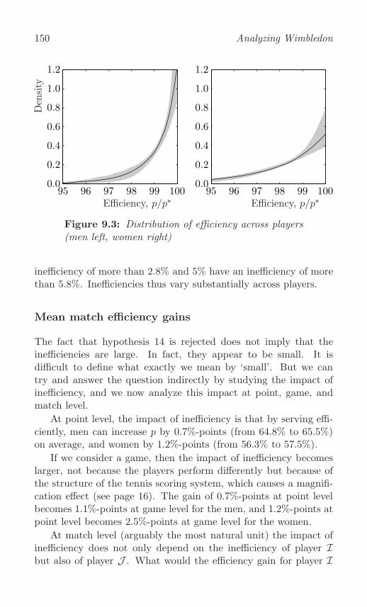
150 Analyzing WimbledonDen
sity
95 96 97 98 99 1000.0
0.2
0.4
0.6
0.8
1.0
1.2
Efficiency, p/p∗95 96 97 98 99 100
0.0
0.2
0.4
0.6
0.8
1.0
1.2
Efficiency, p/p∗
Figure 9.3: Distribution of efficiency across players(men left, women right)
inefficiency of more than 2.8% and 5% have an inefficiency of morethan 5.8%. Inefficiencies thus vary substantially across players.
Mean match efficiency gains
The fact that hypothesis 14 is rejected does not imply that theinefficiencies are large. In fact, they appear to be small. It isdifficult to define what exactly we mean by ‘small’. But we cantry and answer the question indirectly by studying the impact ofinefficiency, and we now analyze this impact at point, game, andmatch level.
At point level, the impact of inefficiency is that by serving effi-ciently, men can increase p by 0.7%-points (from 64.8% to 65.5%)on average, and women by 1.2%-points (from 56.3% to 57.5%).
If we consider a game, then the impact of inefficiency becomeslarger, not because the players perform differently but because ofthe structure of the tennis scoring system, which causes a magnifi-cation effect (see page 16). The gain of 0.7%-points at point levelbecomes 1.1%-points at game level for the men, and 1.2%-points atpoint level becomes 2.5%-points at game level for the women.
At match level (arguably the most natural unit) the impact ofinefficiency does not only depend on the inefficiency of player Ibut also of player J . What would the efficiency gain for player I

Service strategy 151
be if he or she switches to serving efficiently while player J doesnot? The answer is that the mean increase in the probability ofwinning the match is 2.4%-points for the men and 3.2%-points forthe women. This is not so small anymore. If, by serving efficiently,a player can change the match-winning probability from 50-50 to53-47, then this represents a real gain.
Efficiency gains across matches
The mean match efficiency gain averages out differences in efficiencygains across matches. Each match is different and these differencesare ignored by just considering the mean. In a well-balanced match,for example, serving efficiently is expected to be more importantthan in a match where one player is much stronger than the other.This issue is illustrated in Figure 9.4.
Eff.gain,m
∗−
m
0 20 40 60 80 1000
1
2
3
4
5
6
Match-winning prob., m0 20 40 60 80 100
0
1
2
3
4
5
6
Match-winning prob., m
Figure 9.4: Efficiency gain as a function of thematch-winning probability (men left, women right)
For a match between players I and J , Chapter 2 explains howwe can use point-winning probabilities pi and pj to compute theprobability mi (here simply denoted by m) that I wins the match.This is when both players serve normally. If player I serves opti-mally while J continues to serve normally, then the winning prob-ability increases to m∗. Each value of m can be generated by manydifferent combinations of pi and pj, and each combination yields its

152 Analyzing Wimbledon
own value of m and m∗. For each m, there is therefore no uniquevalue of m∗ − m, but rather a whole distribution of values. Thesolid line in the figure presents the median of these values, at eachvalue of m. The figure also contains the 95% confidence intervalaround the median, which again measures the impact of estimationuncertainty.
If two players are approximately of equal strength then the me-dian efficiency gain at match level for the efficient server is 2.7%-points for the men and 4.4%-points for the women. This is themedian gain. In some matches the gain of serving efficiently ismuch higher. For example, 10% of the players in a balanced matchwill have an increase of more than 10%-points in the men’s singles(15%-points in the women’s singles).
In very uneven matches, it does not matter whether the serverincreases the efficiency or not. The figure shows, at m close to zeroor one, that the impact m∗ − m of serving efficiently is virtuallyzero: the top player wins anyway, even when his or her service isnot fully efficient.
Impact on the paycheck
Players play one or more matches in a tournament until they lose.Then they get a paycheck. If by serving efficiently a player wins in-stead of loses the current match (and possibly also the next match),then the prize money may increase substantially, particularly atgrand slam tournaments.
In order to study the monetary impact of serving efficiently,we do a little experiment. We run a hypothetical tournament of128 players (seven rounds, like Wimbledon), where in each matchboth players have probability 50% to win the match, except oneplayer who serves efficiently. We have just seen that for two playersof equal strength the median efficiency gain for the efficient serveris 2.7%-points for the men and 4.4%-points for the women. Wetherefore assume in our experiment that the only efficient player has52.7% (that is, an additional 2.7%-points) probability of winninga match in the men’s singles, and 54.4% in the women’s singles.What is the expected monetary gain for the efficient player?
In grand slam tournaments the paycheck approximately doublesin each round. If we assume that this is exactly true, then the

Service strategy 153
expected paycheck for the efficient player will rise by 18.7% formen and by 32.8% for women. At Wimbledon this would meanan expected additional income of approximately $10,000 for theefficient man and $15,000 for the efficient woman. Hence, eventhough the inefficiency at point level may seem small, the monetarybenefit of efficiency can be substantial.
Why are players inefficient?
We conclude that the service strategy for professional tennis playersin a top tournament is not efficient, and hence that hypothesis 14should be rejected. The rejection of efficiency is not large but its(monetary) effects can be substantial.
Inefficiency is measured by the maximum possible relative in-crease in the probability of winning a point on service, and weestimated it to be 1.1% for men and 2.0% for women on average.The impact of serving efficiently can be quantified at various lev-els of aggregation. At point level the impact is 0.7%-points formen (1.2%-points for women), at game level 1.1%-points (2.5%-points for women), and at match level 2.4%-points (3.2%-points forwomen). These differences reflect the scoring system and the factthat at match level the impact of service efficiency depends on thequality difference between the players. In terms of expected mone-tary gains the expected paycheck for the efficient player could riseby 18.7% for men and 32.8% for women. So even small inefficienciescan have substantial financial consequences. This, in summary, iswhat we found. Higher-ranked players are also more efficient thanlower-ranked players, and the closer the match, the more efficient aplayer serves.
But what is the reason for this inefficiency? Perhaps profes-sional tennis players know their y-curve, but are not able to solvethe optimization problem. Or they correctly solve the optimiza-tion problem, but on the wrong y-curve. From the point of viewof achieving optimality it is much easier for a server to work outthe optimal second service (maximize w(x), as in the hypotheticalcase of a single service) than to work out the optimal first service,because the latter requires knowing the optimal second service. Wewill use this difference to gain further insight into the reasons forinefficiency.

154 Analyzing WimbledonEff.gain,m
∗−
m
0 20 40 60 80 1000
1
2
3
4
5
6
( 1 2)
( 1 2)
( 1 2)
Match-winning prob., m0 20 40 60 80 100
0
1
2
3
4
5
6
( 1 2)
( 1 2)
( 1 2)
Match-winning prob., m
Figure 9.5: Decomposition of efficiency gain intofirst and second service (men left, women right)
Let us separate first-service and second-service efficiency, andask which service is more efficient on average. In Figure 9.5 we plotthree curves for the men (left) and the women (right). The topgraph labeled (x∗1, x
∗2) is the same as the median in Figure 9.4. We
now decompose this graph into (x1, x∗2) where only the second ser-
vice is optimal, and (x∗1, x2) where only the first service is optimal.
What do we see? Players can achieve a larger efficiency gain onthe second service than on the first service, in spite of the fact thatthe second service is conceptually easier to optimize and shouldtherefore be closer to its optimum. The fact that the second ser-vice is less efficient than the first service provides evidence that,although players may be maximizers, they do not maximize thecorrect function.
Rule changes
Rule changes can affect the nature of tennis and the skills requiredto win a match. The International Tennis Federation, in chargeof the Rules, is eager to know the possible impact of rule changeproposals. Can our mathematical model help to predict the effectof rule changes?
The optimal service strategy (x∗1, x∗2) follows from maximizingthe probability of winning a point on service p (x1, x2). Hence, if

Service strategy 155
a rule change does not affect p (x1, x2), then there will be no effecton the optimal strategy. If p (x1, x2) is affected, then the optimalstrategy may well change. To find out how, we need to redo ouroptimization calculations, described on page 142.
Let us reconsider the rule changes discussed in Chapter 2. Nei-ther the match tiebreak of ten points, nor the short set until fourgames, nor the no-ad rule have any impact on p (x1, x2), and hencethe optimal strategy (x∗1, x∗2) is unaffected. This is not surprising,because these proposals only affect the number of points neededto win the match, not the way in which a player can win a point.Adjusting the strategy away from (x∗1, x∗2) in these cases would onlylead to a lower value of p.
Things are different when the second service is abolished, be-cause this rule change does affect the nature of tennis. The questionis what will be the optimal probability x of hitting the single ser-vice in? In terms of our model, what will be the value of x thatmaximizes the probability w(x) of winning a point when using aservice of type x? As derived on page 142, and in line with theanalysis on page 29, the best a player can do is to use the currentsecond service as the only service in the new regime.
Serving in volleyball
Rule changes are rare in tennis, but less rare in many other sports.A comparison with volleyball is of particular interest, because involleyball a rule change occurred that involved the service. Orig-inally, if the serving team won the rally, the team would score apoint, but if they lost the rally, the score would not change butthe service would go to the other team. This is the ‘side-out’ scor-ing system. From 1999 onwards, after pressure to make volleyballfaster-paced and more attractive to television, volleyball uses ‘rally’scoring, in which teams gain a point whenever they win the rally.Many volleyball coaches reacted to this switch by telling their play-ers to be more cautious when serving, because a service fault wouldimmediately give a point to the opponent.
Is this coaching advice correct? Maybe our model can help inanswering this question. Let x be the probability of hitting a ser-vice in, as before, but now for a volleyball team, and let v(x) bethe probability that the serving team wins the rally using a service

156 Analyzing Wimbledon
of type x. In the rally-point system, team I can only win the pointby winning the current rally, and this has probability vi. In theold system (side-out), team I could win a point on service in sev-eral ways. First, by winning the current rally with probability vi.Second, by losing the current rally, winning the next rally on the op-ponent’s serve, and then winning the third rally on its own service.The probability of this event, assuming independence of points, is(1−vi)(1−vj)vi, which we write as vijvi with vij = (1−vi)(1−vj).Third, by losing the own serve, winning the opponent’s serve, losingthe own serve, winning the opponent’s serve, and finally winningthe own serve. The probability of this happening is v2ijvi. In fact,there are infinitely many possibilities. The sum of all correspondingprobabilities is the probability of winning a point:
pi = vi + vijvi + v2ijvi + · · · = vi(1 + vij + v2ij + · · · ) = vi
1− vij.
Since vi and vj are probabilities, they are bounded by zero and one,and we may safely assume that they are not zero or one. Hence0 < vi < 1 and 0 < vj < 1, implying that 0 < vij < 1 and that piin the previous formula is well-defined.
This then is the probability of winning a point on service forteam I in the side-out scoring system. In the rally-point system theprobability is simply pi = vi. This shows that pi is affected by theintroduction of the rally-point system, and hence that the optimalservice strategy x∗ may change. Whether the optimal service infact does change can be found out by the use of a little calculus.
The optimum x∗ is the solution of p′i(x) = 0. Under rally-pointscoring this is the solution of v′i(x) = 0. Determining the optimumunder side-out scoring is more involved. Using the fact that vj doesnot depend on x, we find
p′i(x) =(1− vij)v
′i(x) + viv
′ij(x)
(1− vij)2=
vjv′i(x)
(1− vij)2.
Since vj �= 0 and vij �= 1, the only way that p′i(x) can be zero is thatv′i(x) is zero. But this is the same condition as under rally-pointscoring! Hence the solution x∗ is the same as well. A little math-ematics thus produces the remarkable result that the rule changeaffects the objective function p(x), but not the optimal service strat-egy.

Service strategy 157
What happened to coaching? A year or so after the introductionof rally-point scoring, the coaches realized that being more cautiouswhen serving was the wrong strategy, and they advised players toserve exactly as before. Their initial advice — use a safer service soa higher x — has the benefit of reducing service faults and directpoint losses, but it has the cost that the team will lose the rallymore often if the service is in. Our little model shows that atx = x∗ benefit and cost are balanced in both the side-out systemand the rally-point system. A safer service is ill-advised and willlead to a worse performance.
Further reading
It is slightly amusing and not very realistic to believe that tennisplayers actually calculate partial derivatives and work out optimalstrategy in the way our mathematical development suggests. Inthe context of billiards, Friedman (1953, p. 21) claims that an ex-pert billiard player makes his shot as if he knew the complicatedmathematical formulas that would give the optimum direction oftravel of the balls. It is not that billiard players do the requiredmathematics, but rather that, if they were not playing in this math-ematically optimal way, they would have been beaten too often andnot become top billiard players in the first place.
The literature on service strategy originated with Gale (1971)and George (1973). Many articles followed. The typical approach isto assume two types of services, strong and weak, and then use sum-mary statistics to verify whether the players have chosen the correcttype. Players usually choose ‘strong-weak’, that is, the strong typeas first service and the weak type as second service. But severaltimes an alternative, such as strong-strong, seems better. We knowfrom the discussion on regularity conditions in Table 9.1 and thesubstantial noise in summary statistics (rejection of hypothesis 9)that one should not take the results based on summary statisticstoo literally. The approach in this chapter, based on Klaassen andMagnus (2009), takes the noise issue seriously and allows for a con-tinuum of services a player can choose (instead of just two).
Tennis players, when serving, have to make a number of strate-gic decisions, for example on the speed, the spin, and the directionof the service. Walker and Wooders (2001) examine whether tennis

158 Analyzing Wimbledon
players aim their first service to the receiver’s left or right in anoptimal way. Their results corroborate optimality.
Pollard et al. (2010), Abramitzky et al. (2012), and Clarke andNorman (2012) investigate yet another strategy — regarding chal-lenges. When should a player call upon the Hawk-Eye technologyto arbitrate when he or she disagrees with the umpire’s decision?About 3% of the points played are challenged, with a success rate ofabout 35%. Abramitzky et al. (2012) find that, in line with theory,players are more likely to challenge when the stakes are higher andwhen the (option) value associated with retaining one additionalchallenge is lower. For example, there should be, and there are,more challenges towards the end of a close set. On average, playerstend to challenge too little, but their behavior is close to optimalwhen a simple model is assumed. This corroborates our conclusionon service strategy (page 149).
Why are tennis players so close to optimality? Because theycan be and because they want to be. They can be close to opti-mality, because if they couldn’t they would not play at Wimbledonin the first place. But there is more. Kording (2007) writes thatthe nervous system often comes up with near-optimal decisions inan uncertain world, and he uses tennis as an illustration. So itseems that the human nervous system is well-suited for optimiza-tion problems, of which serving and challenging in tennis are onlysimple examples.
Tennis players are also close to optimality because they want tobe: winning a match at Wimbledon is very rewarding, not only interms of money, but also in terms of world-ranking points and pres-tige. Lallemand et al. (2008) focus on money and demonstrate thatlarger prize differences between winning and losing a tennis matchencourages players to increase effort. Another incentive comes fromclose competition. In uneven matches the gain from playing effi-ciently is low, as Figure 9.4 shows. But in close matches, playersare expected to give the best they can. This is confirmed in Sunde(2009), who shows that tennis players exert less effort in a matchwhere the difference in world rankings is large. In such a match theunderdog often reduces effort because he or she will lose anyway,and the favorite reduces effort as well, because he or she will winanyway. This explains our finding on page 153 that a player servesmore efficiently when the match is closer.

Service strategy 159
It is tempting — and in fact possible as the above studies onincentives and effort show — to relate results on tennis to otherfields. In economics, we could consider payment schemes in firms.Do bonuses based on relative performance — higher bonus if yououtperform your colleague — help to foster the average worker’seffort, as economic theory predicts? The tennis outcomes by Lalle-mand et al. (2008) discussed earlier suggest that they do. Arebonuses less effective when the workers differ in quality? ApplyingSunde’s (2009) and our own tennis results, suggests that they are.Analysis on tennis can thus be useful to study economic problemsthat are difficult to address directly with traditional data. As asecond example, the fact that tighter matches cause players to bemore efficient suggests, more generally, that in a more competitivemarket firms are forced to be more efficient; otherwise they will bedriven out of the market. This supports the view of many policymakers that measures aimed at strengthening market mechanismslead to a more efficient economy. More examples are provided inKlaassen and Magnus (2009).
Examining tennis data helps not only to better understand eco-nomics, but also human behavior in general. Laboratory experi-ments show that humans make suboptimal choices. Such violationsof optimality are often belittled by claiming that the incentiveswere insufficient or that the violations will be eliminated by learn-ing or by market competition. Although Tversky and Kahneman(1986) agree that these factors are relevant, they question whetheraccounting for them would ensure fully optimal choices. In the end,this is an empirical issue. Our tennis data reveal that when incen-tives are high (Wimbledon), competition is fierce, and humans havelearned a lot, then decisions indeed get closer to being optimal. Infact, the small deviations from full efficiency for top tennis playerscome close to an affirmative answer to Tversky and Kahneman’s(1986) question of whether incentives, experience, and competitionensure fully rational choices.
Tennis is not the only sport that can help in understanding andpredicting human behavior, and studies on baseball, basketball, andfootball (both American and soccer) have analyzed favoritism, mar-ket efficiency, optimal labor contracts, racial discrimination, and soon; see the references in Klaassen and Magnus (2009). Sports dataare useful in these studies, because the players’ objectives are clear,

160 Analyzing Wimbledon
incentives to achieve them are strong, players are highly trained,and there is an abundance of high-quality data. Such circumstancesare rare in psychology, economics, and related disciplines, thus mak-ing sports research relevant not only directly for the sport itself butalso indirectly for the behavioral sciences. These advantages applyto tennis in particular: a researcher has to model only one playeragainst one opponent (no team interactions), a good indication ofquality exists due to the world rankings, the existence of two ser-vices doubles the information of a player’s service strategy, andmany points are observed in an objective way. Tennis is ideallysuited for behavioral studies.

10Within a match
So far we have considered matches between two players I and J ,and within each match we have taken all points served by I togetherand also all points served by J . Many hypotheses, however, dependon the development within a match, because they concern specialpoints or special games or ‘momentum’. To test such hypotheses,the probability of winning a point on service must be allowed tovary over points. We therefore leave the analysis at match levelbehind and develop a model at point level. This point-level modelwill serve as our basis in this and the next two chapters.
In the current chapter we develop the point-level model andfocus on two questions: whether points are independent and iden-tically distributed (iid), as used extensively in Chapters 2–4; andwhether new balls are an advantage to the server.
The idea behind the point model
The development of the point model closely follows the develop-ment of the match model, introduced in Chapters 6 and 7 andsummarized on pages 115 and 116. In a match between I and J ,with I serving, the key element in the match model was that theprobability pi of winning a point was split up in an observed partβi, capturing the impact of the players’ rankings, and unobserveddeterminants collected in πi. In formula,
pi = βi + πi.
In the point model we wish to allow for variation in the winningprobability over points, driven by some carefully chosen dynamic

162 Analyzing Wimbledon
variables. At service point t of player I, let dit denote one suchdynamic variable, reflecting for example what happened at the pre-vious service point. (The word ‘dynamic’ signals that dit is notconstant over t.) If the impact of this dynamic variable is denotedby a parameter δ0, then the match model can be extended to apoint model by writing
pit = βi + δ0dit + πi.
Writing pit instead of pi emphasizes that the probability may nowvary over points.
We proceed in three steps. First, we ignore developments withina match (δ0 = 0) and only generalize the analysis from match topoint level, thus obtaining the basic ingredients required for themodel transition. Then we introduce dynamics by allowing δ0 todiffer from zero. And finally we allow for heterogeneity in the im-pact of dynamics, in order to be able to address such questions aswhether momentum matters more or less for top players. In thisfinal step we will substitute δ0 by δi in the same way as we substi-tuted β0 by βi. This will be our baseline model, and it will be usedthroughout this and the next two chapters.
From matches to points
To move from match-level to point-level analysis we first need toreconsider and generalize the moment conditions that determine theparameter estimates. We focus on the probability pit of winning thetth service point. Our Wimbledon data set tells us whether playerI wins or loses the tth service point, and we introduce the variablefit, which takes the value one if the point is won and zero if thepoint is lost.
The first three moment conditions are similar to the ones in thematch model:
E(fit − βi) = 0,
E ((fit − βi)(ri − rj)) = 0,
E ((fit − βi)(ri + rj)) = 0,

Within a match 163
where βi, as before, depends on the ranking difference and the rank-ing sum via
βi = β0 + β−(ri − rj) + β+(ri + rj).
The conditions tell us that winning or losing a point on servicedepends on the rankings of the two players and on an unexplainedpart with mean zero, uncorrelated with the rankings.
The unexplained part consists of unobserved heterogeneity πibetween players and pure noise φit, which now also varies acrosspoints: at some points I is lucky, at other points J . To filter outthe noise we will use the variance of fit and proceed in the same wayas in Chapter 6 (page 97). The data are linked to the probabilityof interest pit by
fit = pit + φit.
Since we ignore dynamics in this section, the probability equationis simply
pit = βi + πi.
Combining the two equations gives
fit = βi + πi + φit.
Because the unexplained part of fit has zero expectation, the sameholds for πi + φit, and we normalize again:
E(πi) = 0, E(φit) = 0.
The random noise φit is not correlated with the winning probability,so that
var(fit) = var(πi) + var(φit),
where var(πi) = σ2 is the structural unobserved variation acrossplayers, that is, the unobserved variation excluding the variation infit arising from noise.
The noise variance var(φit) is restricted in the same way asbefore. In Chapter 6 there were Ti points underlying the frequencyfi. Here we look at just one point in fit, so the restriction becomesthat var(φit) equals the mean of pit(1−pit). In Chapter 6 we rewrotethis restriction in terms of frequencies and divided by Ti − 1. We

164 Analyzing Wimbledon
cannot do this here, because the number of points underlying thefrequency is only one. Instead we write
var(φit) = E (pit(1− pit)) = E ((βi + πi)(1− βi − πi))
= βi(1− βi)− σ2.
The next moment condition then becomes
var(fit) = βi(1− βi).
The final moment in Chapter 6 concerns the correlation. There,we only had to deal with the correlation between the two players Iand J in the match. In the current model we also have correlationbetween all points served by I and all points served by J . Asbefore, we use ρ to denote the correlation between πi and πj. Weassume that the random noise φit is uncorrelated with πi and πj,and also uncorrelated with noise at other points — luck is purelyrandom. Under these assumptions we obtain
cov (πi + φit, πi + φis) = var(πi) = σ2 (s �= t),
cov (πi + φit, πj + φjs) = cov(πi, πj) = ρσ2 (i �= j).
In summary, the six moments for estimating the point model are:
E(fit − βi) = 0,
E ((fit − βi)(ri − rj)) = 0,
E ((fit − βi)(ri + rj)) = 0,
var(fit) = βi(1− βi),
cov (fit, fis) = σ2 (s �= t),
cov (fit, fjs) = ρσ2 (i �= j).
First results at point level
We have now moved from matches to points, but we have not yetintroduced dynamics. Before doing so, let us compare the outcomesof the point model (without dynamics) with the outcomes of thematch model used in previous chapters. We shall leave out tiebreaks

Within a match 165
from the point model — although they were included in the previouschapters — because the service rotation in a tiebreak is differentthan in an ordinary game and this complicates the analysis of thedynamics later in this chapter. As a result, all point models use57,319 points for the men and 28,979 for the women.
β0 β− β+ σ ρmean ri − rj ri + rj heterog. correl.
MenPoint level data 64.6 9.0∗ 2.9∗ 5.6 −0.53Match level data 64.9 8.0∗ 3.1∗ 5.0∗ −0.44∗
WomenPoint level data 55.9 17.1∗ 1.8∗ 4.9 −0.80Match level data 56.3 15.9∗ 1.8◦ 4.2∗ −0.79∗
Table 10.1: Explaining the probability of winning apoint on service: point level versus match level
The model comparison is provided in Table 10.1, which repeatsthe results from Table 7.2 at match level and confronts these withthe new estimates at point level. The results at point level are dif-ferent but not much different from the results at match level. Allconclusions derived from Table 7.2 still hold. For example, we seethat β− > β+ is still true at point level, so that the relative qualityof the two players (quality difference) is more important than thetotal quality (quality sum). Also, the difference in strength betweentop players and lower-ranked players is greater in the women’s sin-gles than in the men’s (larger β− for the women). If we are onlyinterested in static (non-dynamic) results, then match data suffice.But if we wish to analyze dynamic questions, then we require pointdata and an appropriate statistical framework for analyzing them.Having obtained this framework we now move to the second step.
Simple dynamics
In the second step we consider the dynamic setup, be it in its sim-plest form, and introduce a dynamic variable dit to capture variation

166 Analyzing Wimbledon
in pit as the match evolves. This variable is not deterministic, sothat the moment conditions will become more complicated. Theprobability equation of winning service point t now reads
pit = βi + δ0dit + πi,
where δ0 represents the impact (assumed to be constant over allplayers) of the dynamic variable.
Testing iid
In Chapter 2 we introduced hypothesis 1: winning a point on ser-vice is an iid process. What this means is that the probability ofwinning a point is not affected by what happened at earlier points(independence) or by the characteristics of the point (the proba-bility distribution is identical at each point). We have freely usedthe iid assumption throughout the book so far, claiming that it isa reasonable approximation. Now we have the tools to test it.
Let us split the iid hypothesis into two parts: one questioningwhether points are independent, the other whether points are iden-tically distributed. For the identically distributed part we take asour dynamic variable the importance impit of the current point:
d1,it = impit.
Recall from the definition of importance (page 58) that it measuresthe impact of winning instead of losing point t on the probabilityof winning the match. To compute the importance of a point weneed the point probabilities pi and pj. We don’t know these prob-abilities, so they need to be estimated. Obvious candidates for thetwo estimators are βi and βj . Because importance also depends onthe score, it varies across points.
For the independence part we let the dynamic variable be thesuccess or failure at the previous service point:
d2,it = fi,t−1 =
{1 if previous service point was won,
0 if previous service point was lost.
At the first point in a game the previous service point is not thepoint preceding the current point, and we set d2,it = 0 at these

Within a match 167
points. (Alternatively we could have added a correction for thefirst point in a game, but it turns out that such a correction doesnot alter our results, so we prefer the simpler option.)
Static determinants Importance Previous pointβ0 β− β+ δ10 δ20
mean ri − rj ri + rj constant constant
Men 64.4 8.9∗ 2.8∗ −9.8◦ 0.9∗
(0.4) (1.0) (0.7) (6.6) (0.4)
Women 56.0 17.0∗ 1.7∗ −16.4∗ 1.2∗
(0.5) (1.3) (0.8) (7.8) (0.6)
Table 10.2: Impact of importance and previous pointon the probability of winning a service point, simpledynamics
Using these two dynamic variables, our probability equation canbe written as
pit = βi + δ10impit + δ20fi,t−1 + πi,
and Table 10.2 contains the resulting estimates (standard errorsin parentheses). We see that the static parameter estimates arehardly affected by including the dynamic variables: the estimatesof β0, β−, and β+ are almost the same as in Table 10.1. In futuretables we shall therefore no longer report the β-estimates; neitherdo we report the estimates of σ and ρ.
If points are iid, then both δ10 and δ20 should be zero. Table 10.2shows, however, that the importance estimate δ10 is negative, whichmeans that if a point is more important, then the server has lessand the receiver more chance to win the point. The estimate is sig-nificant for women but not for men. The previous-point estimateδ20 is positive, which means that if the previous point was wonthen there is a higher chance of winning the current point as well.Equivalently, if the previous point was lost, then the probability ofwinning the current point is lower. This suggests that swings arepossible in pit, which is an indication of the existence of ‘momen-tum’. We shall have more to say on momentum in Chapter 12.

168 Analyzing Wimbledon
The estimate is significant for both men and women. Overall, theiid hypothesis 1 is rejected both in the men’s and in the women’ssingles, so ups and downs do exist.
Why do players deviate from iid?
First, why do players deviate from the assumption that points areidentically distributed? At important points a player may put moreeffort into the point, but if this is the case then it applies to bothserver and receiver, since the point is equally important to both ofthem. It is not clear why the receiver’s extra effort would dominatethe server’s extra effort. A reason, perhaps, for the lower service-winning probability at important points is that players change theirstyle of play at important points compared to ordinary points. Ifplayers deviate from their normal play and if the normal play isoptimal, then they play suboptimally at important points. If, inaddition, this suboptimality affects the performance of the servermore than the performance of the receiver, then the receiver has anadvantage at important points.
These are many ‘ifs’. Let us test some of them.
Hypothesis 15: Players play safer at important points.
To test this hypothesis, we re-estimate our model but instead oftaking ‘winning the point’ as the variable to be explained, we nowconsider ‘first service in’. The estimates indicate that the impactof importance impit is positive, so more first services go in at im-portant points. We also find fewer aces and fewer double faults atimportant points. We conclude that players serve more conserva-tively under pressure, in line with the hypothesis.
Next, why do they deviate from the assumption that points areindependent? One possibility is that winning the previous pointboosts self-confidence, leading to a winning mood and better play.This could lead to better performance using the same strategy, or itcould lead to a different strategy. In the latter case, a player couldtake more risks than before, which would be bad under normalcircumstances but could be good in different circumstances.
Hypothesis 16: Players take more risks when they are in a win-ning mood.

Within a match 169
We test this hypothesis by considering the estimates of the im-pact of the previous point fi,t−1. Winning the previous point re-duces the probability of hitting the first service in, and increasesthe probabilities of an ace and a double fault. All this suggests thatplayers do take more risks, thus supporting hypothesis 16.
Both identical distribution and independence are therefore re-jected, because players change their style of play: they take lessrisks at important points, but more risks after winning a point. Inaddition, there may be a change in the probability of winning apoint even when we abstract from the changes in the style of play.
Impact of deviations of iid
The rejection from iid is a potential problem for us (the authors),because several sections of this book, in particular Chapters 2–4,are based on the iid assumption. One possible defense of relying onthe iid assumption is that the rejections from iid are not strong: theestimates are only about two standard errors away from zero, so thehypothesis is only marginally rejected. Since we have many obser-vations and only a marginal rejection of the hypothesis, the distinc-tion between significance and relevance, first discussed in Chapter 7,applies here.
Point-winningprob.,pit
-1 -0.5 0 0.5 1 0
20
40
60
80
100
ri − rj-1 -0.5 0 0.5 1
0
20
40
60
80
100
ri − rj
Figure 10.1: Impact of importance on the probabilityof winning a service point for various ranking differ-entials (men left, women right)

170 Analyzing Wimbledon
On the one hand we find that the estimated impact of impor-tance is significant (at least for the women), from which we concludethat points are not identically distributed. On the other hand, ifwe plot the impact of importance in Figure 10.1, then we see thatthis impact is small. The figure plots the predicted pit over the fullrange of ri−rj for the case where the ranking-sum variable ri+rj isset at its average, which is zero due to the centering. The predictedpit is then given by
pit = β0 + β−(ri − rj) + δ10impit + δ20fi,t−1,
which we compute for a range of values of impit covering 95% of itsvalues in the data set, while keeping fi,t−1 fixed at its average. Thisproduces a bundle of lines and we see that this bundle is narrow.Apparently, the predicted value of pit is not much influenced byimpit, even though the estimate of the associated parameter δ10 issignificant. The bundle is wider for the women than for the men,not because the parameter estimate is significant for the women,but because δ10 is larger (in absolute value): −16.4 versus −9.8.
Point-winningprob.,pit
-1 -0.5 0 0.5 1 0
20
40
60
80
100
ri − rj-1 -0.5 0 0.5 1
0
20
40
60
80
100
ri − rj
Figure 10.2: Impact of previous point on the prob-ability of winning a service point for various rankingdifferentials (men left, women right)
Precisely the same story applies to the impact of the previouspoint, as Figure 10.2 illustrates. The same line is drawn as before,but now for fi,t−1 = 1 (previous point is won) and fi,t−1 = 0 (pre-vious point is lost), while keeping impit fixed at its average. The

Within a match 171
resulting two lines are hardly distinguishable indicating that theimpact of fi,t−1 is small.
These two graphs and the analysis accompanying them illustrateagain the important difference between significance and relevance.A deviation may be significant, while the impact of the deviationis negligible and irrelevant.
The small magnitude of the deviations from iid may be surpris-ing to tennis fans. We can all think of matches where momentumseems to have swung from one player to the other. This applies,for example, to the Djokovic-Nadal Australian Open 2012 final, ex-amined on page 96. At 1-1 in sets, the third set was easily won6-2 by Novak Djokovic. It seemed that Rafael Nadal had lost hismomentum. But did he? The answer is that we cannot exclude thepossibility that the 6-2 third set score was just driven by chance.To show that deviations from iid really exist, chance has to be ac-counted for and after doing this, little evidence remains. Comparethe discussion of the drop in Nadal’s first service summary statisticfrom 71% (sets one and two) to 53% (third set), which we analyzedin Chapter 6. As there, we conclude that a seemingly big drop inperformance may have been driven by chance only.
We conclude that the iid hypothesis 1 is rejected. Still, actingas if points are iid provides a reasonable approximation in manyapplications. This is important, because imposing iid simplifiesmany analyses, in particular those in Chapters 2–4.
The baseline model
There is no good reason why the impact of importance and momen-tum should be the same for all players. Therefore, in the third andfinal step of developing the dynamic model, we allow the parametersδ10 and δ20 to vary over players, and generalize them to
δ1i = δ10 + δ1−(ri − rj) + δ1+(ri + rj),
and similarly for δ2i, so that the impacts δ1i and δ2i depend on therankings ri and rj , exactly mimicking the specification of βi. Recallthat (ri−rj) and (ri+rj) are centered, so that δ10 and δ20 representthe impacts for the average match. If δ1− > 0, then the negativeimpact of impit via δ10 is somewhat reduced for servers who have abetter ranking than their opponents. If δ2+ < 0, then the positive

172 Analyzing Wimbledon
impact of fi,t−1 via δ20 is somewhat reduced for servers in a topmatch.
This gives our baseline model, with probability equation
pit = βi + δ1iimpit + δ2ifi,t−1 + πi.
If we let δ0 = δ− = δ+ = 0 for both variables, then we obtain thesetup in the first step (no dynamics), and if we let δ− = δ+ = 0,then we obtain the setup in the second step (simple dynamics).
The baseline model will be our main tool in the remainder ofthis book. In most applications of the model we will add one fur-ther dynamic variable to the model, corresponding to one specifichypothesis under consideration. Only at the end of Chapter 12 shallwe add more than one variable to the baseline model.
Importance Previous point
δ10 δ1− δ1+ δ20 δ2− δ2+mean ri − rj ri + rj mean ri − rj ri + rj
Men −13.0◦ 31.5◦ 42.6∗ 0.9∗ 0.0◦ −2.2∗
Women −16.7∗ 116.3∗ 11.7◦ 1.2∗ 3.3◦ −4.2∗
Table 10.3: Baseline model: impact of importanceand previous point on the probability of winning a ser-vice point
The estimates of the baseline model are given in Table 10.3.These confirm the rejection of iid in hypothesis 1, so that the win-ning probability pit does indeed vary over points. Formally, this isa test on the joint hypothesis that all six δ-parameters (three foreach variable) are zero. The lack of independence and the lack ofidentical distribution both matter in this rejection.
The main contribution of the table concerns the impact acrossplayers. Player homogeneity can be investigated by testing thejoint hypothesis that rankings are irrelevant, both for the impactof importance and for the impact of the previous point, so that themodel of the previous section suffices. The joint test rejects thatδ1−, δ1+, δ2−, and δ2+ are all zero. Deviations from iid are thereforeplayer-dependent.

Within a match 173
When we compare the δ-estimates of men and women, we seethat the signs are the same, which shows that the impacts of impor-tance and previous point work in the same direction in the men’ssingles and in the women’s singles. Equality of the δ-parametersfor these two independent samples is not rejected.
Top players and mental stability
Players are trained by their coaches to be mentally stable, forgetabout the score, forget about the past, and focus on the currentpoint. In other words, they are trained to play points as iid-like aspossible. But maybe not all professionals are equally successful inputting this advice into practice.
Hypothesis 17: Top players are more stable than others.
We study player heterogeneity for both importance and previouspoint in more detail, first importance and then previous point.
Importance
Regarding importance, all estimates in Table 10.3 point in the samedirection, although not all of them are significant. When stakes arehigh and points important, the server has a disadvantage: δ10 < 0.This disadvantage is weaker when the server is a better player thanthe receiver (δ1− > 0). In more detail, if the quality of playerI (measured by ri) increases, then he or she will perform betterat important points (δ1i less negative). Similarly, if the quality ofopponent J increases, then the opponent will perform better atimportant points, so that I will perform worse (δ1i more negative).Hence the players’ rankings work against each other, so that theirimpact on δ1i depends on the difference of the rankings (ri − rj).
If δ1+ were zero, then the above explanation would imply thatthe quality of server I matters as much (in absolute value) as thequality of receiver J . However, the service dominance in tennissuggests that the quality of the server should matter more. Thisexplains why we find δ1+ > 0, because this makes the total impactof ri (measured by δ1− + δ1+ = 74.1 in the men’s singles) strongerin absolute value than the impact of rj (measured by −δ1−+ δ1+ =11.1 in the men’s singles). For the women, the sum of the rankings

174 Analyzing Wimbledon
has a smaller impact, which is consistent with the fact that servicedominance is larger for men than for women.
Impact,δ 1
i
0 0.2 0.4 0.6 0.8 1-100
-50
0
50
100
ri0 0.2 0.4 0.6 0.8 1
-100
-50
0
50
100
ri
Figure 10.3: Relevance of the server’s ranking forthe impact of importance (men left, women right)
To better understand the relevance of the server’s ranking forthe impact of importance, let us consider a server I playing againstan average opponent J . The average opponent will have rj = 0.32for the men and rj = 0.34 for the women, corresponding to worldrankings 43 and 39, respectively. Figure 10.3 illustrates how theestimated impact δ1i of importance depends on the ranking ri. Wesee the estimate (solid line) and its uncertainty (confidence inter-val), indicating that with 95% certainty the true δ1i lies within theband. The vertical reference line is placed at ri = rj , the average.Because the opponent is an average player, δ1i at the point ri = rjis equal to the estimated δ10, that is, −13.0 (just insignificant) forthe men and −16.7 (just significant) for the women. The borderlinesignificance corresponds to the conclusion, earlier in this chapter,that the deviation from iid is not strong. Still, the fact that two in-dependent samples — men and women — yield such similar resultsis reassuring: the importance of a point matters.
The difference in δ1i between the top player with ri = 1 and aweak player with ri = 0 is δ1− + δ1+, which is 74.1 for the men and128.0 for the women, both significant. So if a top player serves atan important point against the average opponent, he or she winsmore often than a weaker player, not only because the strongerplayer wins more points anyway, but also because he or she is moresuccessful at important points.
Is this because the top player can raise his or her level, or be-

Within a match 175
cause the weaker player underperforms, or both? In Figure 10.3 theopponent J is always the average player, while the quality of theserver, player I, varies. We consider three servers: average, top,and weak, respectively. If server I is an average player, then we ob-serve a lower winning probability pit at important points. If playerI underperforms as a server, then he or she will also most likelyunderperform as a receiver. Because players I and J are the same(more precisely, have the same quality), this implies that J alsounderperforms. It could also be that both I outperforms and thatJ outperforms even more, but because the server’s performancemost likely dominates the receiver’s in determining pit, this is nota credible scenario. Hence, both I and J underperform.
Next, consider the top server (at the right side of the graph)at important points. We know that the opponent, the averageplayer, underperforms, which by itself increases pit. So if the topplayer outperforms, pit would increase even more. This does notcorrespond to Figure 10.3, so the top player does not outperform.Underperformance by the top player is not credible, because thisunderperformance would then dominate the underperformance ofthe receiver, leading to a lower pit, contradicting the figure. Thetop player thus plays at his or her normal level at important points.
For the weak server (left side of the graph) we find a reduc-tion in pit. Because the opponent underperforms, which by itselfraises pit, the weak server apparently substantially underperforms.We conclude that below-average players underperform at impor-tant points, and that above-average players are not much affectedby importance. Top players do not perform better, but lower-rankedplayers perform worse, at important points.
Now we can address the identical distribution component ofhypothesis 17, which states that top players are more stable thanweaker players. From the previous discussion we conclude thatfor top players we do not reject identical distribution, but for allmen and women below ranking 50 (ri = 0.3) we do reject identicaldistribution, thus supporting hypothesis 17.
The previous point
Player heterogeneity also matters for the influence of the previouspoint on the current point. Table 10.3 confirms our earlier conclu-

176 Analyzing Wimbledon
sion that winning the previous point increases the probability ofwinning the current point (δ20 > 0) and that losing the previouspoint decreases this probability, both for men and for women. Thenew result is that the stronger the players the weaker the effect(δ2+ < 0). There is no evidence that the ranking difference mat-ters (δ2− = 0). It makes sense that only the sum of the rankingsmatters, because if a stronger player makes the match more stable(less dependence), then this holds for both the server and the re-ceiver. High values of ri and rj now reinforce each other, and this iscaptured by the ranking sum but not by the ranking difference. Iftwo top players meet then the match will be stable, but when twoweaker players meet then there will be more performance swings.(When two amateurs play, there will be many swings, although thisis only based on casual observation without any scientific founda-tion.)
Impact,δ 2
i
0 0.2 0.4 0.6 0.8 1-4
-2
0
2
4
ri0 0.2 0.4 0.6 0.8 1
-4
-2
0
2
4
ri
Figure 10.4: Relevance of the server’s ranking forthe impact of the previous point (men left, womenright)
How much dependence is left for the top players? Do they suc-ceed in switching off the impact from the previous point completelyand ‘forget about the past’? In Figure 10.4 we plot the estimatedδ2i against ri for the average rj . For the average server the es-timated δ2i is just significant for both men and women, so thatwinning (losing) the previous point has a positive (negative) im-pact on the current point. Below-average players also exhibit suchups and downs, but above-average players (including the very topplayers) play the points independently.

Within a match 177
Lessons from the baseline model
Our conclusion is that hypothesis 17 is supported. Top players notonly follow a more efficient service strategy in the match as a whole(see page 153), but they are also more stable across points withina match.
Points in men’s and women’s tennis are not iid, but the devi-ation from iid is not large, and iid will be a good approximationin many directions. Players perform worse on service at importantpoints, but this performance dip is smaller for better players. Per-formance at the previous point carries over to the current point, butabove-average players are able to avoid this effect. For top playerswe do not reject iid; they are stable. But below-average players de-viate from iid in two ways: their performance in the current pointdepends on what happened in the previous point and they are alsoaffected by the importance of a point.
New balls
Tennis as a game has a long history which goes back to the Greeksand Romans. But it was not until 1870 that it became technicallypossible to produce rubber balls which bounce well on grass. WhenThe All England Lawn Tennis and Croquet Club decided to holdtheir first championships in 1877, a three-man subcommittee drewup a set of laws. Rule II stated that
the balls shall be hollow, made of India-rubber, andcovered with white cloth. They shall not be less than2 1/4 inches, nor more than 2 5/8 inches in diameter;and not less than 1 1/4 ounces, nor more than 1 1/2ounces in weight.
The quality of the tennis balls has gradually improved, and cur-rently various types of balls with well-defined characteristics exist.From 1881 to 1901 the balls were supplied by Ayres; thereafter bySlazenger and Sons. Yellow balls were introduced at the hundredthanniversary of the Wimbledon championships in 1986. During the1877 championships 180 balls were used; now more than 50,000.
In 2002 the ITF changed the ball approval from one ball forall surfaces to three ball types: a faster ball (less compression) de-

178 Analyzing Wimbledon
signed to speed up play on slow courts (like clay), a slower ball(slightly larger) designed to reduce the service advantage on fastsurfaces (like grass), and the original ball for medium surfaces (likeacrylic). This freedom to use different types of balls was not asuccess. Players objected to it and the experiment was discontin-ued. All tournaments currently use the medium ball, but there issome evidence that tournaments on slow courts prefer balls at thefaster end of the medium, while tournaments with fast surfaces pre-fer balls at the slower end. Slower balls are also recommended fortennis played at high altitude (above 4000 feet, 1219 meters) as analternative to the pressureless ball.
During a grand slam tennis match new balls are provided afterthe first seven games (to allow for the preliminary warm-up) andthen after each subsequent nine games. Most commentators andmany spectators believe that new balls are an advantage to theserver. But are they right?
Hypothesis 18: New balls are an advantage to the server.
To find out, let us consider Figure 10.5. The age of the balls isindicated from 0 (new balls) to 8 (old balls). The age is 0 in thegame with new balls, 1 in the next game, and so on. After the gamewhere the age of the balls equals 8, new balls are used so that theage is again 0. During the five minutes of warming up before thematch begins, the same balls are used as in the first seven games.Thus it makes sense to set the age of the balls in the first game ofthe match at 2.
Pointfreq.,f i
t
0 2 4 6 850
55
60
65
70
Age of balls0 2 4 6 8
50
55
60
65
70
Age of balls
Figure 10.5: Percentage of service points won de-pending on the age of the balls (men left, women right)
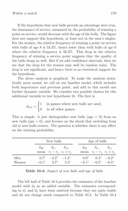
Within a match 179
If the hypothesis that new balls provide an advantage were true,the dominance of service, measured by the probability of winning apoint on service, would decrease with the age of the balls. The figuredoes not support this hypothesis, at least not in the men’s singles.For the women, the relative frequency of winning a point on servicewith balls of age 8 is 53.3%, hence lower than with balls of age 0where the relative frequency is 56.2%. This drop in the relativefrequency of winning a service point suggests that the quality ofthe balls drops as well. But if we add confidence intervals, then wesee that the drop for the women may well be random noise. Thedrop is not significant, and hence there is no statistical support forthe hypothesis.
The above analysis is graphical. To make the analysis statis-tically more sound, we call on our baseline model, which includesboth importance and previous point, and add to this model onefurther dynamic variable. We consider two possible choices for thisadditional variable to test hypothesis 18. The first is
d3,it =
{1 in games where new balls are used,
0 in all other games.
This is simple: it just distinguishes new balls (age = 0) from nonew balls (age > 0), and focuses on the shock that switching fromold to new balls creates. The question is whether there is any effecton the winning probability.
New balls Age of balls
δ30 δ3− δ3+ δ40 δ4− δ4+mean ri − rj ri + rj mean ri − rj ri + rj
Men 0.7◦ −4.2∗ −1.4◦ 0.0◦ 0.4◦ −0.2◦
Women −0.1◦ 3.7◦ 5.4∗ −0.1◦ −0.5◦ −0.5◦
Table 10.4: Impact of new balls and age of balls
The left half of Table 10.4 provides the estimates of the baselinemodel with d3 as an added variable. The estimates correspond-ing to d1 and d2 have been omitted because they are quite stableand do not change much compared to Table 10.3. In Table 10.4

180 Analyzing Wimbledon
most estimates are insignificant (recall that the symbol ◦ denotesinsignificance), and the two significant estimates (denoted by ∗) donot support the hypothesis. We conclude therefore that there is nosupport for hypothesis 18.
Next, we introduce an alternative dynamic variable to test thesame hypothesis,
d4,it = age of the balls (0, . . . , 8).
The variable d4 is more sophisticated than d3, because it distin-guishes between the age of the balls in a gradual manner to capturethe fact that the wear and tear of the balls occurs gradually. Theright half of Table 10.4 presents the estimates of the baseline modelwith d4 as an added variable. Nothing is significant, so hypothe-sis 18 is not supported by the data.
Is there then no difference between new balls and old balls? Yes,there is. New balls, just out of the can, are smooth and bouncy,whereas older balls are softer and fluffier. The older balls providemore grip, making it easier to control the service. More first serviceswill go in and fewer double faults occur. On the other hand, thesmooth new balls travel faster through the air, so that if the firstservice is in, it will have a higher chance of winning the point.
Thus we have two forces working against each other: the prob-ability that the service is in (x in the notation of Chapter 9) de-creases when balls are new, but if the service is in, the probabilityof winning the point (y) increases. What matters is the productxy, and whether this increases or decreases is an empirical issue.We find that the two forces balance each other, so that no new-balladvantage can be found from the data.
Further reading
An extensive literature exists on the question of whether points insports (not only tennis) are identically distributed, and in particularwhether they are independent. ‘Streaks’ in baseball and the ‘hothand’ in basketball are examples of dependence. We will discuss theliterature on identical distribution and independence separately inthe next two chapters. Here we focus on iid in general and on thenew-balls hypothesis in particular.

Within a match 181
The analysis of iid in the current chapter follows Klaassen andMagnus (2001), which is a rather technical paper discussing the es-timation method more fully than we do here. Newton and Aslam(2006) start from the assumption that there exist deviations fromiid. They then model these deviations, simulate their impacts, andreport that, even when relatively strong non-iid effects are intro-duced, results derived from iid are remarkably robust and accurate.This is good news for analyses based on the iid assumption, as inthe early chapters of this book.
Our explanations for deviations from iid — safer play at impor-tant points and riskier play in a winning mood— are more advancedversions of what we reported in Magnus and Klaassen (1996). Inthis earlier paper we found evidence that players at breakpoint optfor safety (more first services in and fewer aces), that after an aceplayers increase risk (fewer first services in and more aces), and thatafter a double fault players take less risks (more first services in andfewer aces). These findings are all in line with our explanations foriid deviations.
A different type of analysis is provided by Paserman (2010),in the context of identical distribution. Paserman uses stroke-by-stroke data from grand slam tournaments played in 2006 and 2007,and finds that at important points, both for men and women, ral-lies last longer, because players hit fewer winners and make fewerunforced errors. He attributes this to a more conservative and lessaggressive playing strategy, and shows that this affects servers morethan receivers. Paserman’s findings support our claim that the sub-optimality caused by too conservative play is larger for the serverthan for the receiver.
Strategic adjustments at important points and in a winningmood derived from tennis data also have implications outside ten-nis, for example in economics. If salaries of agents working in thefinancial sector would contain a bonus and also a substantial maluscomponent, then the consequences of their activities would matterin both directions (like winning or losing a tennis match). Thebehavior of professional tennis players then suggests that top fi-nancial agents will pursue safer actions, reducing the possibility ofa banking crisis. Tennis provides a clean environment to test thistheory.
The quality of the balls matters in professional tennis. Goodwill

182 Analyzing Wimbledon
et al. (2004) simulate trajectories of new (0 impacts) and heavilyworn (1500 impacts) balls, and find that after a typical first servethe worn ball lands about fifty centimeters farther than the newball, because the worn ball does not ‘dip’ as much during the flight.Strict rules exist, available at the website of the ITF TechnicalDepartment, to ensure that the changes in the balls do not havetoo much influence on play. The ITF tests balls in their Tech-nical Centre, a world-leading tennis testing laboratory; see Spurrand Capel-Davies (2007). Despite these strict technical rules, therecould still be a new-ball effect. Our results in the current chaptershow, however, that no effect on the probability of winning a pointon service can be found, in line with Magnus and Klaassen (1999a)and Norton and Clarke (2002). These two papers provide more de-tails, for example regarding the different dimensions of winning aservice point, such as hitting the first service in and winning thepoint given that the first service is in.
11Special points and games
We shall employ the baseline model developed in the previous chap-ter to test some often-heard hypotheses relating to whether or notpoints are identically distributed or independent or both. The nextchapter addresses independence, the current chapter focuses on theissue of identical distribution. There may be more than just dif-ferences in importance, studied in the previous chapter, that makeplayers perform differently across points. Perhaps breakpoints areparticularly special or serving first in a set matters.
Big points
Big points are points that are especially important, such as break-points. It is often claimed that top players perform particularlywell on those points. If true, top players would have a double ad-vantage. Not only are they better players, but they can also raisetheir game when it really matters. We formulate this hypothesis asfollows.
Hypothesis 19: Real champions win the big points.
Let us first think of real champions as seeds and of big pointsas breakpoints, a drastic simplification. When a seed serves inthe men’s singles, the probability of winning a point on service is67.9% at breakpoint down and 68.7% at other points (seeded andnon-seeded receivers taken together). The difference is not signifi-cant. However, when a non-seed serves, the difference is significant:59.3% at breakpoint and 63.5% at other points. Therefore, realchampions perform better at breakpoint down than other players.

184 Analyzing Wimbledon
However, real champions do not win more points at breakpointdown than usual. It is the non-seed who wins fewer points.
The situation is different for the women, where we find no evi-dence for our hypothesis. In the women’s singles, the probability ofwinning a point on service is 58.2% at breakpoint down and 61.7%at other points for a seed (seeded and non-seeded receivers takentogether). For a non-seed these numbers are 50.3% at breakpointdown and 54.8% otherwise. Both differences are significantly nega-tive, and the decrease for the seeds (3.5%-points) is only marginallysmaller than the decrease for the non-seeds (4.5%-points). So,real champions do not perform better than weaker players in thewomen’s singles.
So far we have defined the word ‘champion’ by only looking atthe server: if the server is a seed, then he or she is a champion.What if the receiver is also a seed? As in Chapter 8 we encounterthe problem that only considering the server is too simplistic.
Therefore, as in Chapter 8, we shall distinguish between an ab-solute and a relative interpretation of the word ‘champion’. In anabsolute sense, a player is a real champion if he or she is very good(for example a seed) irrespective of the opponent in the match. Ina relative sense, a player is a real champion if he or she is muchbetter than the opponent, say a seed in a match against a non-seed. Because an absolute champion is typically a better playerthan the opponent, characteristics of relative champions also mat-ter for absolute champions. To exclude this overlap, we again definea cleaned version of absolute champion (corrected for quality differ-ence), and then consider matches between two absolute champions,for example two seeds.
Given these finer distinctions we again consider the question ofwhether champions play their best tennis at breakpoints, and Ta-ble 11.1 provides some of the answers. Regarding absolute champi-ons corrected for quality difference, we compare matches betweentwo seeded players with matches between two non-seeded players.In the men’s singles, a seed playing against another seed will per-form worse at breakpoint down (65.3% against 66.9%), and thesame is true for two non-seeds (60.0% against 64.2%). The differ-ence is bigger for the non-seeds (−4.2 versus −1.6), although notsignificantly so. This is also true in the women’s singles (−5.4 ver-sus 2.1), but there the difference is significant. Hence, there is mild

Special points and games 185
Sd-Sd Sd-NSd NSd-Sd NSd-NSd Total
MenAt breakpoint 65.3 68.9 57.7 60.0 60.9At other points 66.9 69.3 61.3 64.2 64.8Difference −1.6◦ −0.4◦ −3.6∗ −4.2∗ −3.9∗
WomenAt breakpoint 58.7 57.9 48.6 51.0 51.9At other points 56.6 63.5 50.2 56.4 56.6Difference 2.1◦ −5.6∗ −1.6◦ −5.4∗ −4.7∗
Table 11.1: Percentage of points won on service atbreakpoints and other points, seeded (Sd) and non-seeded (NSd) players
confirmation of the hypothesis.
In a relative sense, if the hypothesis were true, a seeded serverwould perform better against a non-seed (Sd-NSd) than a non-seeded server against a seed (NSd-Sd) at breakpoint compared toother points. For the men the seed does perform better, but thedifference of 3.2%-points (−0.4 minus −3.6) is not significant. Forthe women the difference between −5.6 and −1.6 is also not sig-nificant. So, we find no evidence for our hypothesis in a relativesense.
The different interpretations of ‘champion’ lead to mixed re-sults. Maybe this is caused by the fact that our approach is toosimple. Perhaps the quality measure is too simple: we distinguishedonly between Sd and NSd. If a breakpoint occurs in a NSd-NSdmatch, then — given that there are strong and weak non-seeds— the breakpoint may simply indicate that the server is a weakerplayer than the receiver, so that it is quite natural that breakpointsare more often won by the receiver. This should not be interpretedas support for hypothesis 19. We encounter here another exampleof sample selection bias (see page 81): weaker servers are overrepre-sented in the ‘at breakpoint’ sample, and this reduces the estimatedwinning probability. This bias cannot be repaired by only consid-ering non-seeded players; a proper quality measure is required.
Another simplification, and thus another possible reason for the

186 Analyzing Wimbledon
mixed results, is that we distinguished only between breakpointsand non-breakpoints, where all breakpoints are considered equallyimportant and all other points equally unimportant. Here too weneed a finer measure, and this finer measure is available: impor-tance.
Big points and the baseline model
Suppose we generalize the previous model by using our quality vari-able based on expected round (see page 110) instead of seeded ver-sus non-seeded; and our importance measure instead of breakpointsversus non-breakpoints. This would be an improvement, but eventhen the occurrence of a breakpoint could indicate that the re-ceiver is in a winning mood. This would also explain underper-formance at breakpoint down. What is required is a model thatproperly accounts for quality, does not split the sample, accountsfor momentum, and better captures the differences in importanceacross points. This is precisely what our baseline model attemptsto achieve.
The baseline model corrects for quality and contains importance(d1) and previous point (d2). To these two variables we add abreakpoint dummy
d5,it =
{1 if current point is a breakpoint,
0 otherwise.
The extended model thus contains d1, d2, and d5.
δ50 δ5− δ5+mean ri − rj ri + rj
Men −1.3◦ 1.9◦ −2.3◦
Women −2.6∗ −5.7∗ 0.1◦
Table 11.2: Impact of breakpoints
We report the estimates of this model in Table 11.2, but onlyfor d5 because the estimates of the other parameters are roughlysimilar to the ones reported before. Recall from page 130 that the
Special points and games 187
sum (δ− + δ+) captures absolute champions, while δ+ captures theabsolute version corrected for quality differences and δ− capturesrelative champions.
What do we find? In the men’s singles we know from Table 10.3(page 172) that absolute quality matters for the impact of impor-tance (δ1−+ δ1+ > 0). Given this influence, Table 11.2 reveals thatthe occurrence of a breakpoint does not have any further impact:the estimate of δ5− + δ5+ = −0.4, not significant. The same holdsfor the women where the estimate is −5.6, also not significant. If weaccount for quality differences, then the values of δ5+ reveal againthat breakpoints have no additional impact, either for men or forwomen. Regarding relative champions (δ5−) the occurrence of abreakpoint does have further impact, but only for women.
What then is our conclusion regarding hypothesis 19? Is it truethat real champions win the big points or not? Absolute championsperform better at the big points than other players, not becausethey play better tennis than usual but because their opponentsplay worse.
Serving first revisited
In Chapter 2 we briefly discussed hypothesis 2: it is an advantageto serve first in a set. Under the assumption that points are iid —the assumption underlying Chapter 2 — the hypothesis is rejectedon theoretical grounds. Under iid, it makes no difference whetherone serves first in a set or not. However, we have just seen thatthe iid assumption needs to be rejected for below-average players.This does not necessarily imply that it now makes a difference whoserves first in a set, but it does mean that we can no longer reject thehypothesis on theoretical grounds. We should test it empirically.
We start again simply by looking at basic statistics from thedata, not using our statistical model. Our first calculations seemto indicate that hypothesis 2 must be wrong. Overall only 48.2% ofthe sets played in the men’s singles (50.1% in the women’s singles)are won by the player who serves first in the set. Neither of the twopercentages is significantly different from 50%.
Table 11.3 adds a little more detail by looking at individualsets. In the men’s singles, the estimated probabilities of winning aset when serving first is 55.4% in the first set, and 44.3%, 43.5%,

188 Analyzing Wimbledon
Player Winner of previous set
serves first serves first receives first difference
MenSet 1 55.4 − − −Set 2 44.3 72.5 68.0 4.5◦
Set 3 43.5 73.9 72.1 1.8◦
Set 4 51.0 62.9 60.2 2.7◦
Set 5 48.8 48.3 51.0 −2.7◦
WomenSet 1 56.6 − − −Set 2 44.0 72.0 75.2 −3.2◦
Set 3 47.8 63.5 60.1 3.4◦
Table 11.3: Percentage of sets won depending onwhether a player serves first or receives first in a set
51.0%, and 48.8% in the subsequent sets. In the women’s singles,the estimated probabilities of winning a set when serving first is56.6% in the first set, and 44.0% and 47.8% in the second and thirdsets. These numbers suggest that it may be an advantage to servefirst in the first set, but that this advantage becomes a disadvantagein the second and subsequent sets.
Surely this is peculiar. One may doubt that there is an advan-tage in serving first, but if this is not true why should there be anadvantage in receiving first, as there seems to be in the second andsubsequent sets? The answer to this little puzzle is as follows. Theplayer who serves first in a set, if it is not the first set, is usuallythe weaker player. This is so because of a combination of two fac-tors. First, it is likely that the stronger player won the previousset; and second, it is likely that the last game of the previous setwas won by the server. As a result, the loser of the previous settypically serves first in the next set. He or she is then more likelyto lose the current set, not because of a (dis)advantage to servingfirst, but because he or she is the weaker player. The probabilitiesin the second and subsequent sets must be lower than 50%, and theestimated probabilities reflect this. We have failed to correct forquality.

Special points and games 189
To correct for quality and provide a more credible analysis, weemploy conditional rather than unconditional probabilities. Thuswe consider players who have won the previous set, and comparethe estimated probability that they win the current set when serv-ing first with the probability that they win the current set whenreceiving first. The estimates of these conditional probabilities arealso provided in Table 11.3. The difference between the two prob-abilities (serving and receiving) is sometimes estimated as positive,sometimes as negative, but never significant. So now we concludethat there is no service advantage in the second and subsequentsets.
Perhaps there is, however, a possible advantage in the first set.We shall consider this possibility in the next section, but beforedoing so we confront hypothesis 2 with our baseline model. Wetherefore extend the baseline model with the variable
d6,it =
{1 if player I served first in the current set,
0 if player I received first in the current set,
and this leads to the following estimates, again deleting the esti-mates for d1 and d2.
δ60 δ6− δ6+mean ri − rj ri + rj
Men −0.5◦ −0.2◦ 1.7◦
Women 0.4◦ 1.3◦ −6.4∗
Table 11.4: Impact of serving first in a set
Five of the six parameter estimates in Table 11.4 are insignifi-cant. What matters most is that the joint hypothesis
δ60 = δ6− = δ6+ = 0
is not rejected, either for the men or for the women. In this case, themore sophisticated analysis (using the full strength of the baselinemodel) confirms the less sophisticated analysis (using only matchfrequencies). In the less sophisticated analysis we corrected forquality by the noisy ‘winner of the previous set’ indicator. In the
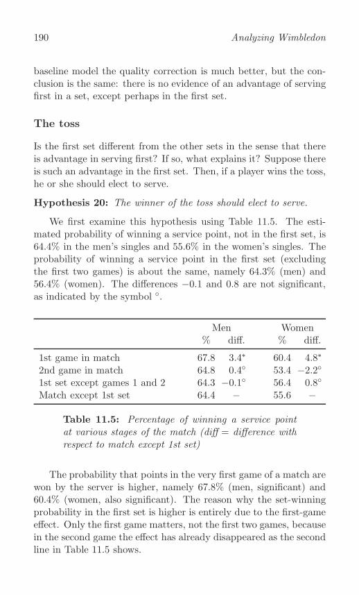
190 Analyzing Wimbledon
baseline model the quality correction is much better, but the con-clusion is the same: there is no evidence of an advantage of servingfirst in a set, except perhaps in the first set.
The toss
Is the first set different from the other sets in the sense that thereis advantage in serving first? If so, what explains it? Suppose thereis such an advantage in the first set. Then, if a player wins the toss,he or she should elect to serve.
Hypothesis 20: The winner of the toss should elect to serve.
We first examine this hypothesis using Table 11.5. The esti-mated probability of winning a service point, not in the first set, is64.4% in the men’s singles and 55.6% in the women’s singles. Theprobability of winning a service point in the first set (excludingthe first two games) is about the same, namely 64.3% (men) and56.4% (women). The differences −0.1 and 0.8 are not significant,as indicated by the symbol ◦.
Men Women% diff. % diff.
1st game in match 67.8 3.4∗ 60.4 4.8∗
2nd game in match 64.8 0.4◦ 53.4 −2.2◦
1st set except games 1 and 2 64.3 −0.1◦ 56.4 0.8◦
Match except 1st set 64.4 − 55.6 −
Table 11.5: Percentage of winning a service pointat various stages of the match (diff = difference withrespect to match except 1st set)
The probability that points in the very first game of a match arewon by the server is higher, namely 67.8% (men, significant) and60.4% (women, also significant). The reason why the set-winningprobability in the first set is higher is entirely due to the first-gameeffect. Only the first game matters, not the first two games, becausein the second game the effect has already disappeared as the secondline in Table 11.5 shows.

Special points and games 191
Hypothesis 20 thus appears to be true. In general, if a playercan choose, he or she should elect to serve first in a match, becausethe very first game of the match is seldom lost by the server and thiscauses a first-set advantage. In fact, this strategy is common amongprofessional players, although choosing to receive is no exception,generally a mistake according to our simple analysis.
There is, however, another possibility. Maybe strong playerselect to serve after winning the toss, while weaker players (not al-ways, but more frequently than stronger players) elect to receive.If this is what happens in practice, than naturally the first gameis won more often by the server than on average, not because ofa first-game advantage, but because the stronger player serves. Inthat case, we would then also expect to see a negative effect in thesecond game, where the weaker player serves, but such an effectdoes not appear to be present. Hence, there is no indication thatstrong players, after winning the toss, elect to serve more often thanweaker players.
Less simplistic and more informative is the approach relying onour baseline model. This time we add the dynamic variable
d7,it =
{1 if service point occurs in first game of match,
0 otherwise,
to our baseline variables d1 and d2. The impact of this additionalvariable is given in Table 11.6.
δ70 δ7− δ7+mean ri − rj ri + rj
Men 3.3∗ 0.2◦ −3.2◦
Women 3.8∗ −6.7◦ −3.0◦
Table 11.6: Impact of serving in the first game ofthe match
The estimate of the impact δ70 is significant and positive, bothfor men and for women. The first-game bonus does not depend onthe rankings (the estimates of δ7− and δ7+ are not significant).
The winner of the toss, irrespective of his or her quality, isapparently rewarded with a 3- to 4%-points higher probability of

192 Analyzing Wimbledon
winning a point in the first game, provided he or she elects to serve.At game level, this advantage is 6- to 8%-points, using the formulaon page 15 and taking 60% as the normal point-winning probability.
The fact that the first game of the match is different from othergames raises the question why this should be the case. We can onlyguess. Maybe the receiver, rather than trying hard to win points inthe first game, learns to read the server’s strategy, judges his or herstrengths and weaknesses, and settles down. But why the receiverin the second game is less passive remains a mystery.
Further reading
The existing literature on testing the identical distribution of pointsfocuses on the impact of importance and breakpoint on the point-winning probability, corresponding to the real champions hypoth-esis 19. The literature is not in agreement, and the differencesbetween the outcomes of the various approaches emphasize againthe importance of a good quality correction.
O’Malley (2008) compares the performance of the server atbreakpoint down to the performance at other points, without cor-recting for quality, and he reports that servers underperform atbreakpoint. Magnus and Klaassen (1999b, 2008) do the same usingthe simplistic quality correction based on seeded and non-seededplayers, and they find the mixed results of Table 11.1. A betterquality correction is proposed in Gonzalez-Dıaz et al. (2012), al-though they still ignore unobserved quality. A second improvementis that they replace the breakpoint dummy by the importance vari-able imp. With these two improvements they study the US Openmen’s singles 1994–2006, and they find the same as reported in thisbook: breakpoint does not matter, importance has some (small)impact, and better players perform better than weaker players atimportant points.

12Momentum
In both the previous and the current chapters we discuss and test anumber of tennis hypotheses, related to the assumption that pointsare independent and identically distributed. In the previous chapterwe concentrated on the identically distributed assumption, now weturn to independence.
Our strategy is the same as in the previous chapter. We firstpresent a simple approach based on averaging, then a more sophisti-cated approach based on our baseline model. Sometimes the resultsfrom the two approaches agree, sometimes they don’t. The base-line model provides the more reliable approach, because it properlyaccounts for quality, importance of a point, and previous-point dy-namics. It also produces more reliable estimates of the precisionsof our estimators.
Both positive and negative dependence between points in amatch should be considered. Winning mood is an example of pos-itive dependence: winning the previous point helps you to win thecurrent point, as we have seen. An example of negative dependenceis the break-rebreak effect. A ‘break’ occurs when a game is notwon by the server but by the receiver. The break-rebreak effect isthe possible effect that a break increases the probability of a re-break. Instead of gaining momentum after the break, the currentserver (receiver in the previous game) is broken back. Does suchan effect exist or it just tennis folklore?
Streaks, the hot hand, and winning mood
A big issue in the statistical analysis of sports is whether ‘momen-tum’ exists. Momentum can only exist when there is dependence,

194 Analyzing Wimbledon
and dependence can occur between matches and between pointswithin a match.
Consider Esther Vergeer, the Dutch wheelchair tennis playerwho won 470 matches in a row, being unbeaten from 2003 untilshe retired in 2013. This is a huge match-winning streak. Herextraordinary talent is one reason for this streak. But perhapsthere is an additional (psychological) reason: the more she wins, thelower is the opponent’s confidence in beating her. While Vergeer’swinning streak relates to dependence between matches, our focuswill be on dependence between points within one match.
Because of her talent, Vergeer wins many consecutive pointsin each match. This is not what we mean by momentum. Mo-mentum is measured conditional on both players’ qualities, andtells us whether, given her and her opponent’s qualities, Vergeerwins more consecutive points than can be explained by randomness.Many will remember the 1993 Wimbledon final between Steffi Grafand Jana Novotna. Novotna led Graf 4-1, 40-30 in the final setwith Novotna on service. Instead of winning her service game, shedouble-faulted and Graf won five consecutive games and the title(one of her twenty-two grand slam victories). This suggests strongdependence between points. One match is, however, not sufficientto prove the existence of dependence in general.
Many studies have addressed momentum in various sports, notonly in tennis but also, and in particular, in basketball and baseball.Dependence between points is called a ‘streak’ in baseball, the ‘hothand’ in basketball, and ‘winning mood’ in tennis. A descriptivestudy focussing on Detroit’s Vinnie Johnson, who has a reputationof being one of the most streaky of all shooters in the National Bas-ketball Association, concluded that he is indeed a streaky shooterand hence that the hot hand exists. But there are other studiesthat find no dependence. The general evidence from the sportsliterature, including tennis, is mixed and inconclusive.
People tend to believe in streaks, because casual observationoverestimates their occurrence. This is a well-established fact. Sup-pose, for example, that you receive a letter on Monday predictingnext Wednesday’s movement of the share prices at the stock ex-change (up or down). The prediction is correct. Next Mondayyou receive another prediction, again correct. This goes on for fiveweeks. Each time the prediction is correct. Then, on Monday in

Momentum 195
week six you are asked to send a check for $100 to receive the nextprediction. Will you send the check? After all, the writer of theletters was right five consecutive times.
From the point of view of the writer of the letters, the experi-ment is easy. He or she selects thirty-two people, and writes to eachof them: half of them predicting ‘up’, the other half ‘down’. Sixteenpeople will have received a correct prediction. To these a second let-ter is sent. Now eight people have received two consecutive correctpredictions. After five weeks, one person remains who has receivedfive consecutive correct predictions. No knowledge about the stockmarket is required. It is pure luck. The probability of five consec-utive successes is 1/32 (about 3%), which is small but not as smallas the general public feels it to be.
Why study tennis?
Testing whether momentum really exists is difficult. Momentum, ifit exists at all, will be small. If the quality of a team (or a player)is underestimated, then there will be more winning streaks by thatteam than expected by pure randomness. As a result, a small errorin measuring quality may lead to the conclusion that momentumexists when in fact it doesn’t. The crux of testing for momentumis to have a good correction for quality and good data.
The features of tennis, combined with our Wimbledon data setand our baseline statistical framework, provide the ideal environ-ment for investigating the possible existence of momentum. Oneimportant advantage is that in tennis singles matches, only twoplayers meet. There are no player substitutions (in contrast tobasketball, say), and this makes it easier to measure quality. Ourdata are on Wimbledon, where the stakes are high and losing somekey points may be decisive for the match outcome. Players havestrong incentives to play their best tennis at each point, which againmakes it easier to control for quality. We have exploited these factsin Chapter 7 to develop a quality correction that uses observables(world ranking) and accounts for unobservables (form of the day).This correction is included in our baseline model.
A second reason why analyzing tennis can contribute to our un-derstanding of momentum is that a tennis match consists of manypoints (in contrast to football, say), and the observations are clean

196 Analyzing Wimbledon
(there is virtually no subjective judgement involved). If momen-tum is small, then a large number of clean observations is requiredto obtain estimates that are sufficiently precise to provide signifi-cant evidence of momentum. Tennis is an ideal setting to test formomentum.
Winning mood in tennis
Momentum in tennis is usually called ‘winning mood’. Winningmood can be defined in many ways. We might, for example, askwhether in a final set (fifth set in the men’s singles, third set inthe women’s singles) the player who has won the previous set hasthe advantage. From our Wimbledon data set, the probability thatthe same player wins the fourth and fifth sets is estimated to be50.2%. In the women’s singles, the estimated probability that thesame player wins the second and third sets is 61.2%. Neither of thetwo percentages is significantly different from 50%, so there appearsto be no basis for this aspect of winning mood.
We shall investigate the possible existence of winning mood, firstby considering the previous service point and then by consideringthe previous ten service points of the current server. Our hypothesisis
Hypothesis 21: Winning mood exists.
As in the previous chapter, we analyze the hypothesis in twoways: simplistic and not so simplistic.
The simplistic approach is based on Table 12.1. Consider aserver in the men’s singles. If he won the previous point in hiscurrent service game, then the overall probability of winning thecurrent point is 65.3%. This is 2.1%-points higher (significant) thanif he lost it. In the women’s singles the effect is even higher witha significant difference of 2.8%-points. The existence of winningmood seems clearly visible.
These overall averages, again, ignore quality differences. Havingwon the previous point may simply indicate that the server is thebetter player, so that he or she will win the current point evenwhen there is no winning mood. One step towards allowing qualitydifferences is to distinguish between seeded and non-seeded players.The effects are generally smaller now, and we notice that the effect

Momentum 197
Sd-Sd Sd-NSd NSd-Sd NSd-NSd Total
MenWon previous point 66.3 70.0 62.3 64.6 65.3Lost previous point 67.5 67.8 59.7 62.7 63.2Difference −1.2◦ 2.2∗ 2.6∗ 1.9∗ 2.1∗
WomenWon previous point 56.0 63.8 50.5 57.6 57.4Lost previous point 56.5 61.6 49.2 54.5 54.6Difference −0.5◦ 2.2∗ 1.3◦ 3.1∗ 2.8∗
Table 12.1: Percentage of points won on service afterserver won or lost previous point (same game), seeded(Sd) and non-seeded (NSd) players
is significant in matches between two non-seeded players, but notin matches between two seeded players. This makes sense. If twoamateurs meet, and one of them misses a point that he or sheshould not have missed, then the resulting anger and frustration islikely to have an effect on the next point(s). The better a player is,the faster can he or she concentrate on the current point and forgetabout the previous point. Table 12.1 confirms this within the groupof professional tennis players.
Still, we should be careful in drawing conclusions from this table,because we cannot really disentangle quality and winning mood byjust looking at averages of matches. As before, a good qualitycorrection is essential and this is where the baseline model comesin.
The baseline model disentangles quality and the effect of theprevious point by including the rankings, unobserved quality, andthe dynamic variable d2,it = fi,t−1, which equals one (zero) in caseof success (failure) at the previous service point. We do not need anew table for this situation, because the estimates in Table 10.3 onpage 172 contain all the necessary information.
We find that the previous-point (momentum) effect is significant(δ20 > 0) for both men and women. The effect in Table 10.3 isabout half the effect in Table 12.1: 0.9 versus 2.1 in the men’ssingles, and 1.2 versus 2.8 in the women’s singles. This is because

198 Analyzing Wimbledon
we now have properly corrected for quality. The incomplete qualitycorrection in the seed/non-seed analysis biases the winning-moodestimate upwardly (sample selection bias), and the baseline modelremoves this bias. We conclude that our data support the idea of awinning mood. There appears to be a weak positive effect, smallerfor top players than for weaker players.
So far we have only looked at the previous point. But this maynot be enough. Perhaps a winning mood is based on more points.Let us consider the previous ten points served by the current server.These ten points approximate the service success in the last twoservice games. This new idea leads to a new dynamic variable,
d8,it = relative frequency of winning the
previous ten service points.
Obviously there is no value for the first ten service points in a matchfor each player. For these points we set d8 equal to the overallaverage winning probability, as estimated in Table 10.1, that is64.6% for the men and 55.9% for the women.
δ80 δ8− δ8+mean ri − rj ri + rj
Men 1.4◦ −0.8◦ −5.9◦
Women −0.4◦ 10.4◦ 9.2◦
Table 12.2: Impact of the previous ten service points
Our model thus includes both the previous-point dummy d2 andthe previous-ten-points dummy d8 (and of course the importancevariable d1). Table 12.2 shows that all estimates associated with d8are insignificant. Adding d8 to the baseline model is therefore notuseful, and our earlier conclusion stands.
Breaks and rebreaks
The server is expected to win his or her service game, particularlyon fast surfaces such as grass. If he or she fails to do so (a servicebreak), this is considered serious in the women’s singles and very

Momentum 199
serious in the men’s singles. A break could therefore have an effecton players in subsequent points.
In Chapter 5 we briefly discussed hypothesis 8: after a break theprobability of being broken back increases. The reason why manycommentators believe in this hypothesis is probably that the currentserver enjoys the success of the break in the previous game andrelaxes a bit, while the opponent is eager to strike back. This wouldinduce a negative correlation, in contrast to the positive correlationassociated with winning mood.
In Table 5.6 (page 81) we found an unexpected and counterintu-itive result. Based on overall averages we concluded not only thatthe hypothesis should be rejected, but even that there is significantevidence that the opposite is true: after a break, the player is morelikely to win his or her own service game. This is contrary to whatcommentators tell us, and we already remarked that the reason forthis result could be that we do not properly account for qualitydifferences.
Sd-Sd Sd-NSd NSd-Sd NSd-NSd Total
MenAfter break 66.7 68.9 60.9 65.6 65.8After no-break 66.7 69.4 61.1 63.4 64.1Difference 0.0◦ −0.5◦ −0.2◦ 2.2∗ 1.7∗
WomenAfter break 56.9 62.9 50.4 57.5 57.9After no-break 56.4 62.9 49.5 54.9 54.9Difference 0.5◦ 0.0◦ 0.9◦ 2.6◦ 3.0∗
Table 12.3: Percentage of winning a service pointdepending on the occurrence of a break in the previousgame (same set), seeded (Sd) and non-seeded (NSd)players
In Table 12.3 we reproduce the overall averages from Table 5.6,and we add a first attempt to allow for quality differences by dis-tinguishing between seeded and non-seeded players. In a matchbetween players of unequal strength (Sd-NSd and NSd-Sd) there

200 Analyzing Wimbledon
is no longer a positive effect. In a match between players of equalstrength (Sd-Sd and NSd-NSd) the effect is also insignificant (ex-cept NSd-NSd for the men). Controlling for quality differencesclearly matters. Maybe a finer quality measure leads to more infor-mative results.
This, again, is where our baseline model enters. We extendthe baseline model with one dynamic variable d9, which shouldcapture the break-rebreak effect. But how should we define thisnew variable? The simplest definition would be: 1 if there was abreak in the previous game (in the same set), and 0 otherwise. Thisdefinition would, however, include situations that are not typical forthe break-rebreak hypothesis, for example a break at 4-0 or a breakat 2-2 following four earlier breaks. What we wish to capture isan unexpected break in the previous game, for example at 3-3 or4-3. After such a break the game score would go to 4-3 or 5-3, adifference of one or two games.
Thus motivated, we capture the break-rebreak effect by themore refined dummy variable
d9,it =
⎧⎪⎪⎪⎪⎨⎪⎪⎪⎪⎩1 if break occurred in previous game,
but not in the game before (same set),
and server leads by one or two games,
0 otherwise.
With this definition, the impact of a break-rebreak, while control-ling for quality, importance, and previous-point dynamics, is sum-marized in Table 12.4.
δ90 δ9− δ9+mean ri − rj ri + rj
Men 0.2◦ −2.1◦ 2.4◦
Women −1.8∗ 0.9◦ 1.1◦
Table 12.4: Impact of break-rebreak dummy
In the men’s singles there is no effect, but in the women’s singlesthere is a break-rebreak effect (δ90 < 0), and this effect is not rank-dependent. This then is our final conclusion: a break-rebreak effect

Momentum 201
is present in the women’s singles but there is no evidence of theeffect in the men’s singles.
Our conclusion for this hypothesis changed several times: froma positive effect in Chapter 5 using overall averages, via a zeroimpact using a quality correction that distinguishes only betweenseeds and non-seeds, to a negative effect (for the women) when wecontrol appropriately for quality. The counterintuitive results fromthe simplistic approaches do not survive a more serious statisticalanalysis.
Missed breakpoints
In the Federer-Nadal 2008 Wimbledon final, Roger Federer was 4-3ahead in the final set and had breakpoint on Rafael Nadal’s ser-vice, but he missed it and Nadal held serve. Two games later at5-4, Federer needed only two points (on Nadal’s serve) to win thechampionship. Nadal held serve, and at 5-5 Federer was two break-points down. Commentators were quick to point out that Federer’sdisappointment of missing the earlier chances had affected the mo-mentum in Nadal’s favor (page 38). Were the commentators rightor wrong in drawing this conclusion?
To find out, we consider the situation where in the previousgame no break has occurred, although the receiver had a goodchance to break because he or she had one or more breakpoints.The receiver did not capitalize on these breakpoints and this mayhave discouraged him or her. Does such a ‘discouragement effect’occur? And, if so, does it influence the performance in the cur-rent game where the discouraged receiver from the previous gameis serving?
Hypothesis 22: After missing breakpoint(s) there is an increasedprobability of being broken in the next game.
Table 12.5 shows no compelling support for this idea. For themen, the probability of winning a point on service after missing allbreakpoints is 0.4%-points lower than usual (1.7%-points for thewomen), in line with the hypothesis but not significant. When webring in quality and distinguish between seeds and non-seeds, thedifferences remain largely insignificant. A simple analysis thereforedoes not support this hypothesis.

202 Analyzing Wimbledon
Sd-Sd Sd-NSd NSd-Sd NSd-NSd Total
MenMissed breakpoints 66.6 70.3 60.2 62.5 63.8No breakpoints 66.8 69.2 61.2 63.6 64.2Difference −0.2◦ 1.1◦ −1.0◦ −1.1◦ −0.4◦
WomenMissed breakpoints 55.5 62.1 50.1 50.9 53.5No breakpoints 56.6 63.1 49.4 55.6 55.2Difference −1.1◦ −1.0◦ 0.7◦ −4.7∗ −1.7◦
Table 12.5: Percentage of winning a service pointdepending on the occurrence of missed breakpoints inthe previous game (same set), seeded (Sd) and non-seeded (NSd) players
The conclusions are different when we employ our baseline model,where we now add the dynamic dummy
d10,it =
⎧⎪⎨⎪⎩1 if breakpoint(s), but no break,
occurred in the previous game (same set),
0 otherwise.
The results are given in Table 12.6. While the evidence is not signif-icant in the men’s singles, there is evidence for the hypothesis in thewomen’s singles: discouragement because of missed breakpoints inthe previous game leads to a smaller probability of winning a pointin the current game (δ10,0 < 0).
Moreover, the fact that δ10− < 0 for the women indicates thatmissing breakpoints against a weaker opponent is particularly harm-ful. This is consistent with the discouragement idea: missing break-points that a player should not have missed, because she is betterthan her opponent, is particularly disappointing.
Finally, δ10+ > 0. This means that if we compare two matcheswith the same quality differential ri − rj, then the better of thetwo matches (highest ri + rj) exhibits the least impact of missedbreakpoints. In fact, in a top match where ri and rj are equal andthe (centered) ri + rj = 0.8, the impact of missed breakpoints isvirtually zero: −3.8+5.4×0.8 = 0.5. This adds support to the idea

Momentum 203
δ10,0 δ10− δ10+mean ri − rj ri + rj
Men −1.2◦ 1.6◦ −0.6◦
Women −3.8∗ −7.8∗ 5.4∗
Table 12.6: Impact of missed breakpoints
that top players are not only technically but also mentally strongerthan other players, thus reinforcing our findings of Chapter 10. Topplayers do not let themselves be discouraged and are less affectedby what happened in the past.
The encompassing model
The restriction d10 = 0 considers two cases jointly: either no break-points occurred in the previous game or a break did occur. It makessense to combine d10 with d9 so that the two cases can be consid-ered separately. Thus we also estimate the baseline model with d9and d10 added jointly rather than separately, but the conclusionsremain the same.
Such analyses provide a check on the robustness of the estima-tion results. This is important, because estimates depend on theassumptions underlying the model, and if those assumptions areviolated inference may become unreliable. The simplistic analy-ses presented in this book and the improved results from applyingbetter methods provide numerous examples of this fact.
Statistical studies typically contain many robustness checks, andwe performed numerous checks to verify that the models used inthis book are robust, that is, not sensitive to small changes in thespecification of the deterministic and random components of themodel. We do not elaborate on these checks, except in the currentsection where we present the estimation results when all dynamicvariables are added to the baseline model. Thus, in Table 12.7,we add to importance (d1) and previous point (d2) the dynamicvariables d3 to d10 jointly, not separately.
When we compare Table 12.7 with the eight tables in Chap-ters 10 to 12 based on including each variable separately, we findremarkable robustness. The results change, but they never change

204 Analyzing Wimbledon
Men Women
δ0 δ− δ+ δ0 δ− δ+mean ri−rj ri+rj mean ri−rj ri+rj
Importance −8.2◦ 32.4◦ 42.7∗ −9.2◦ 121.4∗ 16.6◦
Previous point 0.7◦ 0.3◦ −2.2◦ 0.9◦ 2.3◦ −4.4∗
New balls 1.4◦ −3.2◦ −3.4◦ −0.5◦ 0.6◦ 2.6◦
Age of balls 0.2◦ 0.2◦ −0.5◦ −0.1◦ −0.6◦ −0.5◦
Breakpoint −1.1◦ 1.8◦ −3.2◦ −2.4∗ −4.5◦ 0.4◦
Started serving set −0.7◦ −0.5◦ 1.8◦ 0.0◦ 2.2◦ −6.0∗
First game in match 3.9∗ 0.6◦ −5.2◦ 3.1∗ −10.6∗ −0.3◦
Previous ten points 1.1◦ 0.6◦ −7.1◦ −1.5◦ 11.4◦ 9.5◦
Break-rebreak 0.1◦ −2.0◦ 2.6◦ −2.1∗ −0.5◦ 1.0◦
Missed breakpoints −1.2◦ 1.2◦ −0.3◦ −4.0∗ −8.4∗ 5.0◦
Table 12.7: The encompassing model: impact ofvariables on the probability of winning a service point
so much as to lead to different conclusions. The robustness (lackof sensitivity) is important for the validity of our results, equallyimportant as the statistical significance of our results.
The power of statistics
Sometimes the use of an advanced model makes a difference, some-times it doesn’t. With some of the hypotheses that we have dis-cussed, a simple analysis based on averages provides the same con-clusion as a more sophisticated analysis that appropriately takesaccount of quality and other key variables. But with other hypothe-ses the conclusion changes, and the more sophisticated approach isessential. We do not know in advance how complex we should makeour model.
In Chapter 2 we quoted Albert Einstein, who said: ‘As simpleas possible, but not simpler’. This is very true and very usefulas a basic research philosophy, but it is not easy. The only wayto find out whether an approach is too simple or not is to add‘credible complications’. In this book, these credible complications

Momentum 205
are the GMM approach and the resulting baseline model. On thewhole it appears that simple averaging is too simple, and that thebaseline model and the statistical machinery required to estimateit are really necessary in order to obtain significant, credible, androbust results. Thus, we witness the power of statistics in action.
Further reading
The existence of momentum has been studied in several sports,including tennis, and the relevant literature has been reviewed byBar-Eli et al. (2006) and Reifman (2012). Both reviews find verylittle evidence of the existence of momentum. Athletic streaks, forexample, occur about as often as one would predict by randomchance. The notion of momentum in sports appears to be greatlyoverstated. Despite the limited evidence, many people believe inmomentum. Amos Tversky attempted to fight this common beliefbut without success. ‘I’ve been in a thousand arguments over thistopic, won them all, but convinced no one’, he used to say (quotedin Bar-Eli et al., 2006).
Our analysis suggests that we should distinguish between topplayers and weaker professionals. We find no momentum for thetop players, but we do find some limited momentum for the weakerplayers. Since there are only a few top players and many somewhatweaker players, many matches will have (small) momentum swings.
Dependence between points in baseball, if it exists, is called a‘streak’. Lindsey (1961) concluded that scores can be well repli-cated by assuming independence of runs scored in different innings.Siwoff et al. (1987) found that the probability of hitting well in agame is independent of whether or not the hitter is ‘on a streak’.Albright (1993) agrees and finds no convincing evidence of streakseither. However, in a comment on Albright’s article, Stern andMorris (1993) and Albert (1993) suggested alternative approachesthat might lead to a different conclusion, thus challenging the in-dependence assumption.
In basketball, dependence between points is known as the ‘hothand’. Research on the hot hand originated with Gilovich et al.(1985), who concluded that people believe in the hot hand (notthat a hot hand actually exists). Their results are summarized inKahneman (2011, pp. 116–117) who writes: ‘The hot hand is en-

206 Analyzing Wimbledon
tirely in the eye of the beholders, who are constantly too quick toperceive order and causality in randomness. The hot hand is amassive and widespread cognitive illusion’. Larkey et al. (1989)examined game data for eighteen players from the National Bas-ketball Association, in particular Detroit’s Vinnie Johnson. Fromtheir descriptive analysis they concluded that the hot hand exists.
In tennis, one may ask whether a back-to-the-wall effect exists,where the player who is behind performs better, an illustration ofnegative dependence: failure breeds success. Croucher (1981) foundonly very slight evidence of this effect. Jackson and Mosurski (1997)investigated whether ‘getting slammed during your first set mightaffect your next’. In other words, they challenged the independenceassumption and concluded that there is positive dependence — fail-ure breeds failure — possibly caused by ‘psychological momentum’.
Typical analyses of dependence study how winning or losingpast points or sets affects current performance. In contrast, thebreak-rebreak and missed breakpoint hypotheses 8 and 22 are con-cerned with specific features of those past points. Tests of thesehypotheses (in a less sophisticated framework) were first discussedin Magnus and Klaassen (1996, 1997). These two papers also con-tain tests of related hypotheses not covered in this book.

13The hypotheses revisited
Through this book, like a continuous thread, run twenty-two hy-potheses. These hypotheses are statements on which tennis gurushold strong views: serving first in a set is an advantage, winningmood exists, serving with new balls is an advantage. Of coursewe do not accept the tennis gurus’ wisdoms without solid statisti-cal evidence, and therefore we test the hypotheses using statisticaltechniques, sometimes simple, sometimes more complex. Simpletechniques are sometimes sufficient (which we typically don’t knowuntil we perform a more sophisticated test), sometimes not. Somehypotheses turn out to be true, some are false.
In this final chapter we summarize what we have found. Ouraim is to offer a clear answer, for each of the twenty-two hypothe-ses, to the question of whether the hypothesis is true or false. Thebook contains more than the hypotheses (for example, a discussionof how to forecast the winner of a match and how to choose anoptimal service strategy), but in this chapter we focus on the hy-potheses only. The hypotheses are presented in the same order asthey appear in the book.
In formulating our answers in this chapter, we put clarity abovestatistical cautiousness and subtlety. For example, instead of sayingthat a hypothesis is rejected or not rejected (as statisticians like todo), we shall now simply say that we reject or accept the hypothesis.
1 Winning a point on service is an iid process
Our first hypothesis, not the easiest, is important for our theoret-ical framework, and its outcome matters because later hypotheses

208 Analyzing Wimbledon
(from 15 onwards) only make sense when this first hypothesis isrejected.
What is iid? It means: independent and identically distributed.When points are dependent, then what happened at the previouspoint influences the current point. A missed smash may negativelyaffect the player’s next point, and a series of good points may createa winning mood and affect the next point positively. When pointsare not identically distributed, then a player will be affected by thescore and possibly play more cautiously at important points suchas a breakpoint.
Considering the service points of one player in a singles match,we can ask two questions: are these points independent or not?and are they identically distributed or not? When both effectsare absent, then the service points are independent and identicallydistributed.
If the hypothesis were true, then there would exist no winningmood, no break-rebreak affect (two examples of dependence), andno cautious play at important points (non-identical distribution).Players then play each point ‘as it comes’, without being affectedby what happened at previous points or by the score. Few readerswill believe this and they are right: we find that service points areneither independent nor identically distributed. What is remarkablethough, is not so much this conclusion (which we expected), butrather the fact that the deviation from iid is small.
This immediately raises a further question: is this rejection ofiid true for all players or is there perhaps a difference between topand other players? We shall see later (in hypothesis 17) that thereis indeed a difference, apart from the obvious difference in playingstrength, between top players and other players.
2 It is an advantage to serve first in a set
This hypothesis, our favorite, has been discussed throughout thebook. When we consider individual sets and ask whether the playerwho served first also wins the set, then we find that this is possiblythe case in the first set, but not in any other set. On the contrary, inthe other sets serving first is a disadvantage. This is an unexpectedresult and it holds for both men and women.
The result is unexpected, but it can be explained as follows.

The hypotheses revisited 209
The player who serves first in a set, if it is not the first set, isusually the weaker player. This is so because of a combinationof two factors. First, it is likely that the stronger player won theprevious set; second, it is likely that the last game of the previousset was won by the server. As a result, the loser of the previous settypically serves first in the next set. He or she is then more likelyto lose the current set, not because of a first service (dis)advantage,but because he or she is the weaker player.
It is true therefore that serving first is correlated with losing theset, but it is not true that serving first causes losing the set. Thecause is that the weaker player typically serves first.
To dig deeper we need to adjust for the fact that it is the weakerplayer who typically serves first in a set (if it is not the first set).In other words, we need to take the quality of the players intoaccount. If we do take quality into account (their rankings, formof the day, and so on), then we find that there is no advantage(and no disadvantage) in serving first in a set. So, the hypothesis isrejected, for both men and women. This holds for the second andsubsequent sets. Whether it also holds for the first set remains tobe investigated, and we shall do so in hypothesis 20.
3 Every point (game, set) is equally important toboth players
One often hears: ‘This is an important point, especially for so-and-so’, where so-and-so is typically the player who is behind. If he orshe is down 15-40 in a game, is it perhaps more important for theplayer who is behind to save this breakpoint than for the playerwho is ahead to convert it? No, it is not. Each point is equallyimportant to both players.
No statistical analysis is provided for this hypothesis. It is not aquestion of statistics, but of logic. If there are only two players, thenan advantage for one is automatically a disadvantage for the other:if saving a breakpoint increases the winning probability of the serverby 1%, then it automatically increases the losing probability of thereceiver, also by 1%.
This does not mean that each point is equally important (hy-pothesis 5): some points are more important than other points. Itmeans that if one point is important to the server it is also impor-

210 Analyzing Wimbledon
tant to the receiver. If another point is more important, then it ismore important to both server and receiver.
4 The seventh game is the most important game inthe set
The sonorous tones of Dan Maskell were, for several decades, asmuch a part of Wimbledon as the Duchess of Kent and strawber-ries and cream. When commenting on a particularly exciting pieceof play or an outstanding shot, he sometimes used his most remem-bered and revered catchphrase ‘Oh, I say’, which might well be allhe would say during an entire set.
Maskell was strangely fixated on the seventh game of the set,which he never failed to label ‘all-important’. One way to approachthis hypothesis is to argue that not the seventh game (or indeed anyother game) but the tiebreak is the most important game in a set.Winning or losing the seventh game may be important, but surelywinning or losing the tiebreak is more important. The hypothesisis therefore rejected.
This analysis is correct, but a tiebreak can only be importantwhen there is a tiebreak. Most sets, however, don’t reach 6-6 andtherefore don’t have a tiebreak. A more informative analysis needsto take into account that some games occur less frequently thanothers. If we do that, thus accounting for the fact that the highergame numbers occur less frequently, then we find nothing specialabout the seventh game. So, also from this viewpoint, the hypoth-esis is rejected.
5 All points are equally important
Certainly not. In a game, 0-0 is less important than 30-40. In aset, 0-0 is less important than a tiebreak. In a match, the final setis more important than the first.
Matchpoint is usually not the most important point in a match.For example, at 2-0, 5-0, 40-0, matchpoint is not important atall. The most important point is the point where the swing inthe match-winning probability between winning the point and los-ing it is largest. Points at the end of a tiebreak and breakpointstypically have this property.

The hypotheses revisited 211
6 The probability that the service is in is the same inthe men’s singles as in the women’s singles
Remarkably, the percentage of first and second service in is almostthe same for men and women. On average, the first service is in59.4% of the time for the men and 60.8% for the women, whilethe second service is in 86.4% of the time for men and 86.0% forwomen. The difference between men and women is small (1.4%-point) for the first service and even smaller (0.4%-point) for thesecond service. These percentages are approximations (estimates)of the underlying probabilities. The probabilities themselves cannotbe observed — only the percentages of services in. Can we concludefrom these percentages that the probabilities are the same for menand women?
The degree of complexity of our statistical analysis matters here,and our conclusion differs between first and second service. For thefirst service we conclude that the probability that the service is in isnot the same in the men’s singles as in the women’s singles, in spiteof the fact that 59.4% and 60.8% are close. The percentages areclose but not close enough from a statistical perspective. But forthe second service we conclude that the probability that the serviceis in is the same.
7 The probability of a double fault is the same in themen’s singles as in the women’s singles
Closely related to the previous hypothesis is this statement aboutdouble faults. For the average player we predict 5.52% double faultsfor the men and 5.49% for the women at Wimbledon. These per-centages are very close. How close are the underlying probabilities?Is the probability of a double fault the same in the men’s singles asin the women’s singles? When we test this hypothesis, we acceptit. Hence, men and women have the same probability of serving adouble fault.
How do we reconcile this conclusion with the conclusion fromthe previous hypothesis, in particular the fact that the probabilityof first service in is not the same for men and women? One reasonis estimation uncertainty. A double fault occurs when both the

212 Analyzing Wimbledon
first service and the second service are a fault. As a result, theprobability of a double fault depends on both the first-service-inand the second-service-in probabilities. In the previous hypothesiswe accepted one thing (second-service-in probability is the samefor men and women), while we rejected the other (first-service-inprobability is not the same for men and women). Whether or not wereject the combination (same probability of a double fault) dependson the estimation uncertainty associated with both the first and thesecond service. In this case, the combined estimation uncertaintyis so large that we cannot reject the combined hypothesis. Thus weconclude that men and women have the same probability of servinga double fault.
8 After a break the probability of being broken backincreases
Unexpected conclusions can emerge when we do not analyze thedata in a statistically sound manner. We saw this throughout thebook, for example in hypothesis 2, where we asked whether it isan advantage to serve first in a set. The famous break-rebreakhypothesis provides another example.
If the hypothesis is true, then the probability of winning a ser-vice game decreases after a break of the opponent’s service in theprevious game (in the same set), so that a rebreak becomes moreprobable. A simple analysis reveals that the probability of winninga service game is 3.3%-points higher if a break occurred in the pre-vious game than if no break occurred. This is for the men; for thewomen the difference is 5.7%-points, even higher. Apparently, aftera break the probability of being broken back decreases rather thanincreases.
Of course it does, if we don’t take quality into account! Thebetter player breaks the opponent’s service and holds his or herown service, not because a break makes it easier to hold service,but because he or she is the better player.
When we correct for quality, then we find no effect in the men’ssingles but we do find an effect in the women’s singles: women whohave broken their opponent’s service should be extra careful not tolose their own service game. So, we reject the hypothesis for menbut accept it for women.

The hypotheses revisited 213
9 Summary statistics give a precise impression of aplayer’s performance
Our data set is large and clean, so one would expect that summarystatistics involving all matches are informative. This is indeed thecase. But let us consider just one match, say the Djokovic-NadalAustralian Open 2012 final. The viewer is presented after eachset with summary statistics of that set and of the match. Howinformative are these statistics?
In the Djokovic-Nadal match, the first two sets were long andclose. Djokovic lost the first set 5-7 and won the second 6-4. Thethird set was short and Djokovic won it 6-2, suggesting a dip inNadal’s performance. But was this dip structural or was it justchance?
Nadal’s first-service percentage dropped from 71% in the firsttwo sets to 53% in the third set. It would be tempting to concludethat Nadal took more risks on his first service in the third set, andthat it would be better to take less risks to get the percentage upagain in the fourth set. However, realizing that the percentages arebased on ninety-two points (in the first two sets) and only thirty(in the third set), the statistically correct conclusion is that thereis no evidence that Nadal changed anything. The difference inpercentages can easily be explained by chance. Hence, to concludefrom these percentages that Nadal changed his service strategy inthe third set is not justified from a statistical viewpoint.
This does not mean that summary statistics are useless. Theyreflect what actually happened and they are entertaining. How-ever, due to the presence of chance, they do not equal but onlyapproximate a player’s underlying performance, and the smallerthe number of points on which the summary statistic is based, thelarger is the relevance of chance, and the poorer is the approxima-tion. In general, summary statistics on individual matches do notgive a precise impression of a player’s performance.
10 Quality is a pyramid
The ‘quality’ of a player is obviously important in explaining hisor her success. How to take quality into account requires carefulmodeling, as we have seen in hypotheses 2 (advantage of serving

214 Analyzing Wimbledon
first in a set) and 8 (break-rebreak effect), and failure to do so canlead to unexpected results. Quality is partly observed (through theranking) and partly unobserved (form of the day, small injuries,fear of a specific opponent). Unobserved quality can be accountedfor, even in the absence of data, and we elaborate on this subtleissue in this book. The question underlying the current hypothesis,however, deals with observed rather than with unobserved quality:how do we measure observed quality?
The data consist of the ranking points for each player, publishedweekly by the ATP (for men) and WTA (for women). The 2012end-of-year lists show Novak Djokovic (12,920 points) and VictoriaAzarenka (10,595 points) as the world’s number one at the endof 2012. The same two lists show that there are five players in themen’s singles (three in the women’s singles) who have between 2000and 2500 points, seven (thirteen) between 1500 and 2000 points,seventeen (thirty-two) between 1000 and 1500 points, and seventy-three (seventy-eight) between 500 and 1000 points. So, going downfrom the top by steps of 500 points each involves more and moreplayers. This is what we mean by a pyramid, and a more detailedanalysis confirms that quality is indeed a pyramid.
This also helps in answering the next question: how do we mea-sure quality? The ranking points lead to a ranking (1, 2, . . . ) andwe could say: quality equals ranking. This would not be a gooddefinition, however, because it would imply that the difference instrength between, say, numbers 1 and 16 is the same as the differ-ence between 101 and 116, and we know now that this is not thecase.
We could also say: quality equals ranking points. This wouldlead to a pyramid, but not necessarily the best pyramid. A problemwith this definition is also that the method of computing rankingpoints changes regularly and is not the same for men and women.In this book we developed our own formula for quality, obviously apyramid based on the rankings.
Our formula is based on the idea of ‘expected round’. Theexpected round is a number associated with the ranking: 8 for aplayer with ranki = 1 who is expected to reach the final (round 7)and win, 7 for a player with ranki = 2 who is expected to reach thefinal and lose, 6 for players with ranki 3 or 4 who are expected tolose in round 6, 5 for players with ranki 5 to 8 who are expected

The hypotheses revisited 215
to lose in round 5, and so on. When we walk down the pyramid,more and more players get the same quality indicator, capturingthe flattening of quality differences represented by the idea of apyramid. A problem with the expected round, however, is that itdoes not distinguish between, for example, players ranked 9 to 16,because all of them are expected to lose in round 4. Our formula —a smoothed version of expected round — provides expected-roundnumbers for all rankings, is a pyramid, and captures the essence ofquality.
11 Top players must grow into the tournament
For a top player in an early round, the actual round will be smallerthan the expected round based on his or her ranking. Does the topplayer perform according to his or her expected round or somewhatless good, because he or she has to grow into the tournament? Thereis no evidence of this in our data set. Professional tennis, especiallyat grand slam tournaments, is so competitive that top players cannot and do not relax in the early rounds.
12 Men’s tennis is more competitive than women’stennis
This is true. Since men play the best-of-five sets and women thebest-of-three, one would expect fewer upsets in the men’s singlesthan in the women’s singles: the longer the match format, the morelikely it is that the favorite will win. However, when we considerthe data, we see that more upsets (top-sixteen seeds not reachingthe last sixteen) occur in the men’s singles than in the women’ssingles. Men’s tennis is therefore more competitive than women’stennis, and a more sophisticated statistical analysis confirms thisconclusion.
In recent years, women’s tennis has become more competitive.The world’s number-one position has changed regularly and manydifferent women have won one or more of the grand slam tourna-ments. In contrast, men’s tennis has been dominated by just fourplayers: Novak Djokovic, Roger Federer, Rafael Nadal, and AndyMurray. Casual observation may suggest that men’s tennis is nolonger more competitive than women’s tennis. This suggestion is

216 Analyzing Wimbledon
not supported by the data. While it is true that the competitivegap between men’s and women’s tennis has become smaller, it isstill the case that men’s tennis is more competitive than women’stennis.
13 A player is as good as his or her second service
To investigate this often-heard hypothesis we first need to definewhen a second service is ‘good’. A (first or second) service is ‘good’when the percentage of points won on that service is high. Re-markably, this characteristic is typically not shown on television.The characteristics shown are the percentages ‘1st (2nd) service in’and ‘points won if 1st (2nd) service is in’. But it is not these twoprobabilities themselves which matter most — it is their product.Hence, a second service is good if the product of the percentages‘2nd service in’ and ‘points won if 2nd service is in’ is high.
Next we need to define what we mean by a ‘good’ player, anddetermine what type of matches are therefore appropriate to testthe hypothesis. We could compare matches between a seeded serveragainst any opponent with matches between a non-seeded serveragainst any opponent. The server in the first type of match is abetter player than the server in the second type, and this allows usto test the hypothesis by checking whether the seeded server winsmore points on second service than on first service compared to thenon-seeded server.
The previous comparison distinguishes between the quality ofservers, but it does not distinguish between the quality of receivers.If we wish to allow for this distinction as well, we should comparematches between a seeded server against a seeded receiver withmatches between a non-seeded server against a non-seeded oppo-nent. As a third possibility we could compare matches between aseeded server against a non-seeded opponent with matches betweena non-seeded server against a seeded opponent.
The three types of matches correspond with different interpreta-tions of the hypothesis. We analyze each type separately, not onlyusing the rough distinction seeded versus non-seeded, but in par-ticular using a finer distinction based on our definition of quality.We conclude that a player is indeed as good as his or her secondservice.

The hypotheses revisited 217
14 Players have an efficient service strategy
Each server in a tennis match chooses that strategy which maxi-mizes the probability of winning a point. A good strategy involvesmaking both services neither too easy (in which case the receiverwill kill it) nor too difficult (in which case the service will too oftenbe a fault). In this book we developed a model to answer the ques-tion how difficult a player should make his or her service in orderto maximize the probability of winning a service point. With thismodel we can compute the optimal service strategy and compareit to the actual strategy. The ratio between the actual probabilityand the optimal probability is the ‘efficiency’, a number betweenzero and one. If the ratio equals one, then there is full efficiency.Of course, the efficiency differs per player and depends also on theopponent.
For a player in a given match, the efficiency could be one, butmore likely it will be lower than one. How much lower? We findthat the average efficiency is 98.9% for the men and 98.0% for thewomen. This is pretty efficient, but not fully efficient, and we rejectthe hypothesis.
We reject the hypothesis, but our method also allows us to quan-tify the inefficiency: 1.1% for men and 2.0% for women. Apparently,the women are less efficient than the men, at least in choosing theirservice strategy. We also find that 25% of the men have an inef-ficiency of more than 1.4% and that 25% of the women have aninefficiency of more than 2.8%.
Inefficiencies thus vary substantially across players. This vari-ation is not pure chance; there is structure in it. Higher-rankedplayers are more efficient than lower-ranked players: they are notonly better tennis players, but they also make better choices aboutwhat type of service to use.
15 Players play safer at important points
In hypothesis 1 we saw that it is not the case that players play ‘onepoint at a time’, that is, we rejected the hypothesis that points areiid. In fact, service points are both dependent and non-identicallydistributed, although the deviations from iid are small. In the re-maining hypotheses of this chapter we try to discover more about

218 Analyzing Wimbledon
these deviations.
Players may be tempted to serve with less risks at importantpoints, in order to make sure that the first service is in and toavoid a double fault. And indeed we find, at important points, thatmore first services go in, and fewer aces and double faults occur.Players serve more conservatively under pressure: they play saferat important points.
However, not all players are the same. Maybe some players arenot affected by important points. This key question is discussedbelow in hypothesis 17.
16 Players take more risks when they are in a winningmood
While the previous hypothesis provided an example of how playersdeviate from the assumption that points are identically distributed,the current hypothesis asks why players deviate from the assump-tion that points are independent. Players do indeed take more riskswhen they are in a winning mood. Winning the previous point re-duces the probability of hitting the first service in, and it increasesthe probability of an ace, but also of a double fault.
Here, too, we may ask whether this result holds for all playersor whether we can distinguish between different types of players.Maybe some players are not affected by a winning mood. Thisquestion is taken up in the next hypothesis.
17 Top players are more stable than others
Players are trained by their coaches to be mentally stable, forgetabout the score, forget about the past, and focus on the currentpoint. In other words, they are trained to play points as iid-like aspossible. But maybe not all professionals are equally successful inputting this advice into practice. This is true. Top players play likeiid, but the lower a player is on the rankings the further he or shedeviates from iid. Top players are indeed more stable.
Let us investigate both aspects of iid, first the identical distri-bution aspect, then the independence. If a top player serves at animportant point against a weaker opponent, he or she wins moreoften than a weaker player would, not only because the stronger

The hypotheses revisited 219
player wins more points anyway, but also because he or she is moresuccessful at important points. This is not because the top playerraises his or her level, but because the weaker player underperforms.Top players are not affected by the importance of a point. Theyplay as if they are ignorant about the score. For top players, servicepoints are identically distributed.
Next, the independence aspect. For a weak (not top) server,winning the previous point has a positive impact on the currentpoint, and losing it has a negative impact. This is the case for bothmen and women. But top players play the points independently.They are able to switch off the impact from the previous pointand ‘forget about the past’. For top players, service points areindependent.
In contrast, weaker players deviate from iid in two ways: theirperformance at the current point depends on what happened at theprevious point (not independent) and they are also affected by theimportance of a point (not identically distributed).
Top players are, of course, better players than weaker play-ers. But they have, in addition, two advantages that are unrelatedto their service power and technique. They are more stable thanweaker players and, as we have seen in hypothesis 14, they also havea more efficient service strategy.
18 New balls are an advantage to the server
At grand slam tournaments, six new balls are provided at the be-ginning of the warm-up, then after the first seven games, and thenafter every nine games. It may seem unlikely that the character-istics of the balls change in such a short lifespan. Still, this is thecase.
New balls, just out of the can, are smooth and bouncy, whereasused balls are softer and fluffier. The used balls provide more grip,making it easier to control the service. More first services will goin and fewer double faults occur. On the other hand, the smoothnew balls travel faster through the air, so that if the first service isin, the server will have a higher chance of winning the point.
Thus we have two forces working against each other: the proba-bility that the service is in decreases when balls are new, but if theservice is in, the probability of winning the point increases. These

220 Analyzing Wimbledon
two forces turn out to possess about the same strength, so that theycancel each other out and no new-ball advantage can be found fromthe data.
19 Real champions win the big points
Closely related to hypothesis 17 is the current hypothesis, whichrelates to the identical distribution of service points. We alreadyknow that points are not identically distributed. We also know(hypothesis 15) that most players play safer at big points, that is,at points that are especially important, such as breakpoints andpoints at the end of a close set.
Is it true that top players perform particularly well on thosepoints? Yes and no. The top players are more successful thanweaker players, but not because they play better. What happensis that their opponents play worse. This gives the top players adouble advantage. Not only are they better players, but they arealso more stable under pressure (as we have seen in hypothesis 17),while the opposition underperforms when it really matters.
20 The winner of the toss should elect to serve
In hypothesis 2 we saw that there is no advantage in serving firstin a set, except possibly in the first set. We find that the winner ofthe toss, if he or she elects to serve, has a 3- to 4%-points higherprobability of winning a point in the first game, irrespective of hisor her quality. This effect exists only in the first game, not in thefirst two games as one might think. Hence, in general, the winnerof the toss should elect to serve.
21 Winning mood exists
The final two hypotheses are concerned with (in)dependence. Inhypothesis 16 we found that players take more risks when they arein a winning mood, that is, after winning the previous service point.But what exactly is a winning mood (also known as ‘momentum’)and does it actually exist? This is a big issue in sport statistics, notjust in tennis but in all sports, and it has been studied extensively,particularly in baseball (streaks) and basketball (hot hand). All

The hypotheses revisited 221
commentators and almost all spectators believe in it, but that doesnot mean that it actually exists.
If we define winning mood by only considering the previousservice point, then we find evidence of a winning mood because ofa previous-point effect, both for men and for women. Our datathus support the idea of a winning mood. The effect is small, muchsmaller than most spectators believe it to be. When we distinguishbetween top players and somewhat weaker players, then no winning-mood effect for top players and a small but nontrivial effect forsomewhat weaker players can be detected.
One might object that there is more to winning mood than justwinning the previous point. This is a reasonable objection, butif we consider not one but ten previous service points (about twoservice games), then we reach the same conclusion.
22 After missing breakpoint(s) there is an increasedprobability of being broken in the next game
In hypothesis 8 we studied the impact of a break in the previousgame on the performance of the server in the current game. Supposenow that no break occurred in the previous game, but that thereceiver had a good chance to break because he or she had oneor more breakpoints. The receiver did not, however, capitalize onthese breakpoints and this may have discouraged him or her. Doessuch a ‘discouragement effect’ occur? And, if so, does it affectthe current game where the discouraged receiver from the previousgame is serving?
There is no support for this hypothesis in the men’s singles, butthere is support in the women’s singles. Moreover, in the women’ssingles, the weaker the opponent, the larger is the discouragementeffect of missing breakpoints.
This discouragement effect is smaller at high-level matches (say,between two top players) than at lower-level matches. Top players,women as well as men, are not only technically but also mentallystronger than other players. They do not let themselves be discour-aged and are less affected by what happened in the past.

This page intentionally left blank

ATennis rules and terms
In this appendix we briefly summarize the rules of tennis and pro-vide a glossary of some tennis terms used in this book that maynot be familiar to all readers. The International Tennis Federation(ITF) is the governing body of tennis and determines the Rules ofTennis. The latest Rules can be downloaded from the ITF website(www.itftennis.com). A more elaborate overview of tennis termi-nology is available on many websites.
Tennis rules
Amatch consists of sets, a set consists of games, and a game consistsof points. A singles match is contested between two players. Theserver of the first game is decided by a coin toss. Thereafter, eachsuccessive game is served by the other player.
At the beginning of each point one player, the server, hits theball to the opponent, the receiver. When the service is a fault,the server hits a second service. When the second service is also afault, the server loses the point. When the first or second serviceis in, the rally begins. The rally ends when a player fails to hit theball into the correct court before it bounces twice consecutively, inwhich case that player loses the point.
A game is finished when one player wins at least four pointswith a difference of at least two points. The points are counted as0 (‘love’), 15, 30, 40 (rather than as 0, 1, 2, 3). When the score isa tie at 40-all, it is called ‘deuce’. When the server wins (or loses)the point after deuce, it is advantage to the server (or receiver).When the player with advantage wins the next point he/she winsthe game; otherwise the score is deuce again.

224 Analyzing Wimbledon
A tiebreak is a special type of game. It is won when a playerreaches at least seven points and has a lead of two or more points.In contrast to standard games, points in a tiebreak are counted 0,1, 2, . . . The player who received in the preceding game serves firstin the tiebreak. After the first point the service alternates everytwo points.
A set is finished when one player wins at least six games witha difference of at least two games. When the score reaches 6-6,either the set continues until a two-game difference is achieved orit is decided by a tiebreak, depending on tournament rules. In thelatter case the possible winning scores in a set are: 6-0, 6-1, 6-2,6-3, 6-4, 7-5, or 7-6.
A match consists of a maximum of three or five sets. Women’smatches are always best-of-three sets whereas men’s matches areeither best-of-three or best-of-five, depending on tournament rules.
Tennis terms
Ace: Service where the ball is served in and not touched by thereceiver.
Ad court: Left side of the court of each player, so called becausethe ‘ad’ (‘advantage’) point is served to this side of the court.See also deuce court.
Advantage: Score in a game where a player has won the point atdeuce and therefore needs one more point to win the game.
Break (of service): Game won by the receiving player.
Break back: See rebreak.
Breakpoint: Point which, if won by the receiver, results in a breakof service.
Challenge: Protest where a player requests an official review of thespot where the ball has landed, using electronic ball-trackingtechnology; see Hawk-Eye. Challenges are only available insome tournaments and at some courts.
Deuce: Score of 40-40 in a game.

Tennis rules and terms 225
Deuce court: Right side of the court of each player, so called be-cause at deuce the point is served to this side of the court.
Double fault: Two service faults in a row within one point, caus-ing the player serving to lose the point.
Doubles: Matches played by four players, two on each side.
Final set: Third set in a best-of-three match; fifth set in a best-of-five match.
Gamepoint: Score where the server needs one more point to winthe game. See also breakpoint.
Grand slam: The grand slam tournaments are the four majortournaments in a calendar year: the Australian Open, theFrench Open (or Roland Garros), Wimbledon, and the USOpen.
Hawk-Eye: Computer system connected to cameras to track thepath of the ball for replay purposes.
Hold (service): To win the game when serving. Compare break.
In: A ball is in if, after leaving the racket, it first hits the correctcourt. For example, a service is in if the ball first hits theservice court diagonally opposite.
Matchpoint: Score where a player needs one more point to winthe match.
Rally: Following the service, a series of hits that ends when thepoint is decided.
Ranking (world ranking): Official ordering of players, updatedweekly, based on the number of points he or she accrued dur-ing the past year. The best player is ranked number one.
Rebreak: To win a game as the receiving player immediately afterlosing the previous game as the serving player.
Receiver: Player who is being served to.

226 Analyzing Wimbledon
Seed: Highly-ranked player whose position in a tournament hasbeen arranged based on his/her ranking so as not to meetother highly-ranked players in the early rounds of play. Fora given tournament there is a specified number of seeds, de-pending on the size of the draw. For ATP/WTA tournaments,typically one out of four players are seeds.
Server: Player who is serving.
Service (serve): Every point begins with a serve where the serverattempts to hit the ball over the net into the service courtdiagonally opposite.
Service court: On each side of the net there are two service courts:left and right. These are boxes bounded by the singles side-lines, the serviceline, and the center serviceline.
Service game: With regard to a player, the game in which theplayer is serving (e.g., ‘player I won a service game on love’means that I won a game where (s)he was serving withoutthe opponent scoring a point).
Setpoint: Score where a player needs one more point to win a set.
Singles: Matches played by two players, one on each side.
Tiebreak: Special game played when the score is 6-6 in a set todecide the winner of the set.
Toss: Before the beginning of a match a coin is tossed, usually bythe umpire. The toss decides the choice of ends and the choiceto be server or receiver in the first game.
Unseeded player: Player who is not a seed in a tournament.
Winning mood: Mental condition of a player after being success-ful in the preceding points or games, possibly leading to ahigher probability of being successful at the current point.

BList of symbols
In this second appendix we list all symbols used in the book, orderedby type. We have aimed for consistency in notation, realizing thatcomplete consistency, even if possible, is not desirable because itcomes at the cost of too many qualifiers.
In a typical tennis match, two players I and J are competingagainst each other. Many variables thus depend on i (correspond-ing to I) and j (corresponding to J ). For notational simplicitywe typically leave out the j index. The index t for the servicepoint number is also often left out, particularly when a variable isconstant over time.
Winning probabilities
p, pi, pit probability that I wins a point on servicep∗ optimal/efficient value of pp average p over all matches in a tournamentg, gi probability that I wins a service gamegi probability that I wins a service game
under the no-ad rulesi probability that I wins a setm, mi probability that I wins the matchmi(a, b) probability that I wins the match from set score a-bm∗ value of m if I serves optimallyv, vi probability that team I wins a rally on service
(in volleyball)vij (1− vi)(1− vj) (in volleyball)

228 Analyzing Wimbledon
Score probabilities and importance
a-b point, game, or set score of I (score a)against J (score b)
imp, imppm, impit importance of point in matchimppg, imppg(a, b) importance of point score a-b in game
impgs, impgs(a, b) importance of game score a-b in set
impgs(n) importance of game number n in set
impsm, impsm(a, b) importance of set score a-b in match�(a, b) probability of reaching game score a-b in set�(n) probability that game number n occurs in set
Point scores in a game are counted as 0, 15, 30, 40, advantage, whilegames and sets are counted as 0, 1, 2, . . . .
Service probabilities
w1 probability of winning a point on first servicew2 probability of winning a point on second servicew(x) probability of winning a point on service
using service of type xx probability that the service is inx1, x1i, x2, x2i probability that the first (second) service is iny1, y1i, y2, y2i probability of winning a point on first (second)
service given that the service is iny(x) probability of winning a point on service
given that the service of type x is inx∗1, x∗2, y∗1, y∗2 optimal/efficient values corresponding to
x1, x2, y1, y2, respectively
Quality
bonusi quality gain of low-ranked player I who hasprogressed further in the tournament than expected
malusi quality loss of high-ranked player Iin the early stage of the tournament
qi (observed) quality of player Iri stage in the tournament in which player I is expected
to lose, based only on ranki

List of symbols 229
ranki official (ATP/WTA) ranking of player Iroundi round in which I plays current match
Operators
E expectationvar variancecov covariancesd standard deviationse standard error∑
summation operator
Miscellaneous variables
bi decimal betting odds for Idit dynamic determinant of pitdiff difference between two probabilitiesf , fi, fit relative frequency that I wins a point on serviceM number of moment restrictions in GMM estimationN total number of matches in the samplen game number in a setTi number of points served by I in the matchT total number of points in the sample
Random/unexplained parts
π, πi unexplained quality part of p, piφ, φi, φit random noise in f , fi, fit, respectively
Note that we use Greek letters for random variables correspondingto the equivalent Latin-letter variables.
Parameters
αb, αm impact of bonusi and malusi on qiβ0 mean of piβ−, β+ impact of ri − rj and ri + rj on piβS , βR impact of ri (server) and rj (receiver)
on ace and double fault probabilities

230 Analyzing Wimbledon
γ0, γ1, λ intercept, slope, and curvature of the y(x)-curveδ0 mean impact of a dynamic variable on pitδ−, δ+ effect of ri − rj and ri + rj on the impact of a
dynamic variable dit on pitρ correlation coefficient between πi and πj
(correlation between opponents)σ2 variance of πi (player heterogeneity)
Miscellaneous symbols
◦ not significant∗ in a table: significant at 5% level;
attached to a probability: optimal/efficient valueˆ estimator, estimate
m subscript when match is the unit of analysis

CData, software, and mathematical derivations
In this appendix we draw the reader’s attention to our respectivewebsites
www.uva.nl/profile/f.j.g.m.klaassen
and
www.janmagnus.nl/misc/wimbledon.pdf,
where we provide background material. This material includes thecomplete data set underlying most of our analyses; the computerprogram, called Richard, which we use to calculate probabilitiesand importances; and also derivations of some of the mathematicalresults.
Data
The principal (but not the only) data set used in this book consistsof point-by-point data of men’s and women’s singles matches atWimbledon 1992–1995. These data were given to us by IBM UK,and they were supplemented by ranking data, which we receivedfrom the ITF. The data set is described and applied in Chapter 5.Chapters 6–9 use match data, aggregated from these point data.The point data themselves are used again in Chapters 10–12.
The complete data set is presented as an Excel file. This filealso contains point-by-point data of the three matches (Federer-Nadal, Clijsters-Williams, Djokovic-Nadal) investigated in Chap-ters 3 and 4. Included in the Excel file is a separate sheet wherethe user can easily calculate most of the simple estimates presented
232 Analyzing Wimbledon
in the book, that is, the estimates that do not rely on the GMMestimation method. GMM estimation requires external statisticalsoftware.
As an example, consider the relative frequency of winning apoint on service for the men. The overall estimate of 64.4% andthe standard error of 0.2%, presented on page 71, is replicated inthe file. The output automatically provides the breakdown of thisfrequency, based on whether the server and receiver are seeded ornon-seeded players, as reported in Table 7.1. If the user wishesto analyze only a subsample, for example excluding points in atiebreak and after a break in the previous game within the sameset (as used in Table 12.3), he or she can enter this request as well.Precise instructions and explanations are provided in the file.
At several places in the book we also use other data. Summarystatistics of the grand slam tournaments from 1992–2010 were pro-vided by IBM UK and the ITF. Data from OnCourt are used inanalyzing upsets and the Isner-Mahut match in Chapter 2, andin performing sensitivity analyses for two of the three matches inChapter 3. The bookmakers’ odds at the beginning of each of thethree matches were downloaded from Tennis-data.
More tennis data can be obtained from various sources. Thewebsites of the grand slam tournaments provide data and illustra-tions using IBM SlamTracker. The ATP and WTA websites containdata on many tournaments and rankings. Other websites publishdata as well, and their number is growing.
Software: program Richard
Richard is a computer program. It computes the probabilities ofwinning the game (tiebreak), set, and match at any point of a tennismatch. The program also produces functions of these probabilities,such as the importance of a game in the set or the importance of apoint in the match.
The required inputs are the service point winning probabilitiespi and pj of the two players I and J , the current score, the currentserver, and the rules of the tournament (say, best-of-five sets witha tiebreak in all sets except the final set), but nothing more. Theprogram is fast, accurate, has a convenient ‘matrix’ setup, is flexiblefor studying rule changes, and it is freely available.

Data, software, and mathematical derivations 233
Richard was born in 1994. It was first written in a computerlanguage called Turbo Pascal. Since Turbo Pascal is not muchused any more, we present the program in Matlab, which is morecommon and more user-friendly.
The program, including all source code, can be downloaded fromour websites. Also available on the websites is the associated ‘inver-sion’ program, described on page 34, which is important for in-playforecasting and betting. The inversion program produces robustvalues of pi and pj, based on two inputs: the match-winning prob-ability at the beginning of the match (obtained from an outsidesource) and the sum pi + pj.
We emphasize three features of Richard. First, it is based onthe assumption that service points are independent and identi-cally distributed (iid), so that two probabilities (pi and pj) suffice.Since tennis has a hierarchical structure (points form games andtiebreaks, which form sets, which form matches), games, tiebreaksand sets are also iid. This allows for a step-by-step calculationof the probability of winning a match. First calculate the game(tiebreak) winning probability, then the set probability, and finallythe match probability.
A second distinguishing feature of Richard concerns the calcula-tion of the winning probabilities at each step. For example, considera game served by player I. At score 0-0, I can win or lose the point,giving 15-0 or 0-15, with probabilities pi and 1 − pi, respectively.After 15-0 the score can be 30-0 or 15-15, with the same transi-tion probabilities, and similarly after 0-15. Special scores are deuceand advantage. Deuce is equivalent to 30-30, and advantage server(receiver) is equivalent to 40-30 (30-40). The game continues untileither I or J has won the game. We thus obtain seventeen differentscores and at each score the probability of the next score is con-stant: either pi or 1−pi. This type of structure is known as a ‘finiteMarkov chain’ (Kemeny and Snell, 1960, pp. 161–167), which hasmany important and useful properties. One of these properties isthat the whole process can be represented in one square of numbers,called a ‘matrix’. This matrix has seventeen rows and seventeencolumns, and each cell contains the probability of going from onescore to the other. Given this matrix, it is then easy to calculatethe probability of winning the game from each score. The matrixapproach makes the program fast: a few hundredths of a second

234 Analyzing Wimbledon
to compute one match-winning probability. The total computingtime for all 413 points in the Federer-Nadal Wimbledon 2008 finalis only two seconds on a standard desktop computer.
Third, the program is not only fast, but also flexible. Winningprobabilities under non-standard rules (match tiebreak, four-gameset, no-ad rule), as discussed on page 27, can be obtained by justchanging one single number. Because the full source code is avail-able, the user can adjust the code, if needed, to investigate other,more exotic, rule changes.
Mathematical derivations
For almost all mathematical results in the book we have explainedhow they were derived and why we needed them. For the remain-ing formulas we provide full derivations on our websites. Theseremaining formulas are the following.
Chapter 2
(a) In Section ‘From point to game’ we consider a game whereplayer I is serving with constant probability pi of winning a point.The probability that he or she wins the game is expressed by theformula for gi on page 15.
(b) Section ‘Long matches: Isner-Mahut 2010’ (pages 24–27) con-tains a three-step derivation. This derivation is complete, but thereader may wish to see the explicit expressions (and their deriva-tions) of �(5, 5) and �(a, b). These are provided on the websites.
(c) In Section ‘Rule changes: the no-ad rule’ we consider the situa-tion where the traditional scoring system at deuce is replaced by theno-ad rule, so that only one deciding point is played at deuce, andwe state that the probability that I wins the game would changefrom gi to gi on page 28.
Chapter 4
In Section ‘Big points in a game’ (pages 50–52) we consider againa game where player I is serving with probability pi of winning

Data, software, and mathematical derivations 235
a service point. Then we present formulas for imppg(40, 30), theimportance of the score 40-30, and for imppg(30, 40), the importanceof the score 30-40.
Chapter 9
At the end of Section ‘Impact on the paycheck’ (page 153) we statethat if the paycheck doubles in each round, then the expected pay-check for the efficient player will rise by 18.7% for men and by 32.8%for women.

This page intentionally left blank

Bibliography
There exists an extensive literature on tennis and tennis statistics.This bibliography only provides the references to the literature dis-cussed in the ‘further reading’ sections. It does not attempt to coverthe whole literature.
Abramitzky, R., L. Einav, S. Kolkowitz, and R. Mill (2012). Onthe optimality of line call challenges in professional tennis,International Economic Review, 53, 939–963.
Albert, J.H. (1993). Comment on ‘A statistical analysis of hittingstreaks in baseball’ by S.C. Albright, Journal of the AmericanStatistical Association, 88, 1184–1188.
Albert, J., J. Bennett, and J.J. Cochran (Eds) (2005). Anthol-ogy of Statistics in Sports, ASA-SIAM Series on Statisticsand Applied Probability, SIAM, Philadelphia, PA and ASA,Alexandria, VA.
Albright, S.C. (1993). A statistical analysis of hitting streaks inbaseball (including comments and rejoinder), Journal of theAmerican Statistical Association, 88, 1175–1196.
Anderson, L.R. (1982). Sex differences on a conjunctive task:Mixed-doubles tennis teams, Personality and Social Psychol-ogy Bulletin, 8, 330–335.
Bar-Eli, M., S. Avugos, and M. Raab (2006). Twenty years of ‘hothand’ research: Review and critique, Psychology of Sport andExercise, 7, 525–553.
Barnett, T. (2006). Mathematical Modelling in Hierarchical Gameswith Specific Reference to Tennis, PhD thesis, Swinburne Uni-versity of Technology, Melbourne.

238 Bibliography
Bedford, A., T. Barnett, G.H. Pollard, and G.N. Pollard (2010).How the interpretation of match statistics affects player per-formance, Journal of Medicine and Science in Tennis, 15,23–27.
Blackman, S.S. and J.W. Casey (1980). Development of a ratingsystem for all tennis players, Operations Research, 28, 489–502.
Boulier, B.L. and H.O. Stekler (1999). Are sports seedings goodpredictors?: An evaluation, International Journal of Forecast-ing, 15, 83–91.
Brody, H., R. Cross, and C. Lindsey (2002). The Physics andTechnology of Tennis, The United States Racquet StringersAssociation, Vista, CA.
Clarke, S.R. (2011). Rating non-elite tennis players using teamdoubles competition results, Journal of the Operational Re-search Society, 62, 1385–1390.
Clarke, S.R. and D. Dyte (2000). Using official ratings to simu-late major tennis tournaments, International Transactions inOperational Research, 7, 585–594.
Clarke, S.R. and J.M. Norman (2012). Optimal challenges in ten-nis. Journal of the Operational Research Society, 63, 1765–1772.
Coate, D. and D. Robbins (2001). The tournament careers of top-ranked men and women tennis professionals: Are the gen-tlemen more committed than the ladies?, Journal of LaborResearch, 22, 185–193.
Coe, A. (2000). The balance between technology and tradition intennis, in: Tennis Science & Technology (Eds S.J. Haake andA. Coe), Blackwell Science, Oxford, pp. 3–40.
Collins, B. (2010). The Bud Collins History of Tennis, 2nd Edi-tion, New Chapter Press, New York.
Crespo, M., M. Reid, and A. Quinn (2006). Tennis Psychology:200+ Practical Drills and the Latest Research, InternationalTennis Federation, London.
Croucher, J.S. (1981). An analysis of the first 100 years of Wim-bledon tennis finals, Teaching Statistics, 3, 72–75.

Bibliography 239
Croucher, J.S. (1998). Developing strategies in tennis, in: Statis-tics in Sport (Ed J. Bennett), Arnold, London, pp. 157–171.
Davies, M., L. Pitt, D. Shapiro, and R. Watson (2005). Bet-fair.com: Five technology forces revolutionize worldwide wa-gering, European Management Journal, 23, 533–541.
Del Corral, J. (2009). Competitive balance and match uncertaintyin grand-slam tennis: Effects of seeding system, gender, andcourt surface, Journal of Sports Economics, 10, 563–581.
Del Corral, J. and J. Prieto-Rodrıguez (2010). Are differences inranks good predictors for grand slam tennis matches?, Inter-national Journal of Forecasting, 26, 551–563.
Dobson, S. and J. Goddard (2011). The Economics of Football,2nd Edition, Cambridge University Press, New York.
Dudink, A. (1994). Birth date and sporting success, Nature, 368,592.
Easton, S. and K. Uylangco (2010). Forecasting outcomes in tennismatches using within-match betting markets, InternationalJournal of Forecasting, 26, 564–575.
Edgar, S. and P. O’Donoghue (2005). Season of birth distributionof elite tennis players, Journal of Sports Sciences, 23, 1013–1020.
Elliott, B., Reid, M., and M. Crespo (2009). Technique Develop-ment in Tennis Stroke Production, International Tennis Fed-eration, London.
Friedman, M. (1953). Essays in Positive Economics, Chicago Uni-versity Press, Chicago.
Gale, D. (1971). Optimal strategy for serving in tennis. Mathe-matics Magazine, 44, 197–199.
Garicano, L., Palacios-Huerta, I., and C. Prendergast (2005). Fa-voritism under social pressure, The Review of Economics andStatistics, 87, 208–216.
George, S.L. (1973). Optimal strategy in tennis: A simple proba-bilistic model, Applied Statistics, 22, 97–104.
Gilovich, T., R. Vallone, and A. Tversky (1985). The hot handin basketball: On the misperception of random sequences,Cognitive Psychology, 17, 295–314.

240 Bibliography
Gonzalez-Dıaz, J., O. Grossner, and B.W. Rogers (2012). Per-forming best when it matters most: Evidence from profes-sional tennis, Journal of Economic Behavior & Organization,84, 767–781.
Goodwill, S.R., S.B. Chin, and S.J. Haake (2004). Aerodynamicsof spinning and non-spinning tennis balls, Journal of WindEngineering and Industrial Aerodynamics, 92, 935–958.
Guillaume, M., S. Len, M. Tafflet, L. Quinquis, B. Montalvan, K.Schaal, H. Nassif, F.D. Desgorces, and J.-F. Toussaint (2011).Success and decline: Top 10 tennis players follow a biphasiccourse, Medicine & Science in Sports & Exercise, 43, 2148–2154.
Hall, A.R. (2005). Generalized Method of Moments, Oxford Uni-versity Press, New York.
Hart, A. (1997). Agatha Christie’s Miss Marple: The Life andTimes of Miss Jane Marple, Harper Collins Publishers, Lon-don.
Holder, R.L. and A.M. Nevill (1997). Modelling performance atinternational tennis and golf tournaments: Is there a homeadvantage?, The Statistician, 46, 551–559.
Holtzen, D.W. (2000). Handedness and professional tennis, Inter-national Journal of Neuroscience, 105, 101–119.
Hsi, B.P. and D.M. Burych (1971). Games of two players, AppliedStatistics, 20, 86–92.
Humphreys, M. (2011). Wizardry: Baseball’s All-Time GreatestFielders Revealed, Oxford University Press, New York.
Jackson, D.A. (1994). Index betting on sports, The Statistician,43, 309–315.
Jackson D. and K. Mosurski (1997). Heavy defeats in tennis: Psy-chological momentum of random effect, Chance, 10, 27–34.
Kahneman, D. (2011). Thinking, Fast and Slow, Penguin BooksLtd, London.
Kemeny, J.G. and J.L. Snell (1960). Finite Markov Chains, VanNostrand, Princeton, NJ.
Klaassen, F.J.G.M. and J.R. Magnus (2000). How to reduce theservice dominance in tennis? Empirical results from four yearsat Wimbledon, in: Tennis Science & Technology (Eds S.J.

Bibliography 241
Haake and A.O. Coe), Blackwell Science, Oxford, pp. 277–284.
Klaassen, F.J.G.M. and J.R. Magnus (2001). Are points in tennisindependent and identically distributed? Evidence from adynamic binary panel data model, Journal of the AmericanStatistical Association, 96, 500–509.
Klaassen, F.J.G.M. and J.R. Magnus (2003a). Forecasting thewinner of a tennis match, European Journal of OperationalResearch, 148, 257–267.
Klaassen, F.J.G.M. and J.R. Magnus (2003b). On the probabilityof winning a tennis match, Medicine and Science in Tennis,8, No. 3, 10–11.
Klaassen, F.J.G.M. and J.R. Magnus (2003c). Forecasting in ten-nis, in: Tennis Science & Technology 2 (Ed S. Miller), Inter-national Tennis Federation, London, pp. 333–340.
Klaassen, F.J.G.M. and J.R. Magnus (2008). De kans om een ten-niswedstrijd te winnen: Federer-Nadal in de finale van Wim-bledon 2007, Stator, 9, No. 2, 8–11.
Klaassen, F.J.G.M. and J.R. Magnus (2009). The efficiency oftop agents: An analysis through service strategy in tennis,Journal of Econometrics, 148, 72–85.
Koning, R.H. (2009). Sport and measurement of competition, DeEconomist, 157, 229–249.
Koning, R.H. (2011). Home advantage in professional tennis,Journal of Sports Sciences, 29, 19–27.
Kording, K. (2007). Decision theory: What ‘should’ the nervoussystem do?, Science, 318, 606–610.
Lake, R.J. (2011). Social class, etiquette and behavioural restraintin British lawn tennis, 1870–1939, The International Journalof the History of Sport, 28, 876–894.
Lallemand, T., R. Plasman, and F. Rycx (2008). Women andcompetition in elimination tournaments: Evidence from pro-fessional tennis data, Journal of Sports Economics, 9, 3–19.
Larkey, P., R. Smith, and J. Kadane (1989). It’s okay to believein the ‘hot hand’, Chance, 2, 22–30.

242 Bibliography
Lindsey, G.R. (1961). The progress of the score during a baseballgame, Journal of the American Statistical Association, 56,703–728.
Little, A. (1995). Wimbledon Compendium 1995, The All EnglandLawn Tennis and Croquet Club, London.
Magnus, J.R. and F.J.G.M. Klaassen (1995). De professor weetwat commentatoren niet weten, De Volkskrant, October 14.
Magnus, J.R. and F.J.G.M. Klaassen (1996). Testing some com-mon tennis hypotheses: Four years at Wimbledon, Center forEconomic Research, Discussion Paper 1996-73, Tilburg Uni-versity, The Netherlands.
Magnus, J.R. and F.J.G.M. Klaassen (1997). Wat tenniscommen-tatoren niet weten: Een analyse van vier jaar Wimbledon,Kwantitatieve Methoden, 18, No. 54, 55–62. Reply in: Kwan-titatieve Methoden, 18, No. 54, 67.
Magnus, J.R. and F.J.G.M. Klaassen (1999a). The effect of newballs in tennis: Four years at Wimbledon, The Statistician(Journal of the Royal Statistical Society, Series D), 48, 239–246.
Magnus, J.R. and F.J.G.M. Klaassen (1999b). On the advantageof serving first in a tennis set: Four years at Wimbledon, TheStatistician (Journal of the Royal Statistical Society, SeriesD), 48, 247–256.
Magnus, J.R. and F.J.G.M. Klaassen (1999c). The final set in atennis match: Four years at Wimbledon, Journal of AppliedStatistics, 26, 461–468.
Magnus, J.R. and F.J.G.M. Klaassen (2008). Myths in tennis, in:Statistical Thinking in Sports (Eds J. Albert and R.H. Kon-ing), Chapman & Hall/CRC Press, Boca Raton, FL, Chap-ter 13, pp. 217–240.
McHale, I. and A. Morton (2011). A Bradley-Terry type modelfor forecasting tennis match results, International Journal ofForecasting, 27, 619–630.
Mehta, R., F. Alam, and A. Subic (2008). Review of tennis ballaerodynamics. Sports Technology, 1, 7–16.
Miles, R.E. (1984). Symmetric sequential analysis: The efficienciesof sports scoring systems (with particular reference to those

Bibliography 243
of tennis), Journal of the Royal Statistical Society, Series B,46, 93–108.
Miller, S. (2006). Modern tennis rackets, balls, and surfaces,British Journal of Sports Medicine, 40, 401–405.
Morris, C. (1977). The most important points in tennis, in: Opti-mal Strategies in Sports (Eds S.P. Ladany and R.E. Machol),North-Holland Publishing Company, Amsterdam, pp. 131–140.
Newton, P.K. and K. Aslam (2006). Monte Carlo tennis, SIAMReview, 48, 722–742.
Newton, P.K. and J.B. Keller (2005). Probability of winning attennis I: Theory and data, Studies in Applied Mathematics,114, 241–269.
Norton, P. and S.R. Clarke (2002). Serving up some grand slamtennis statistics, Proceedings of the Sixth Australian Confer-ence on Mathematics and Computers in Sport (Eds G.L. Co-hen and T.N. Langtry), Bond University, Queensland, Aus-tralia, 1–3 July 2002, pp. 202–209.
O’Donoghue, P. and B. Ingram (2001). A notational analysis ofelite tennis strategy, Journal of Sports Sciences, 19, 107–115.
O’Malley, A.J. (2008). Probability formulas and statistical anal-ysis in tennis, Journal of Quantitative Analysis in Sports, 4,1–21.
Paserman, M.D. (2010). Gender differences in performance incompetitive environments? Evidence from professional tennisplayers, Boston University and Hebrew University, mimeo.
Pluim, B., S. Miller, D. Dines, P. Renstrom, G. Windler, B. Norris,K. Stroia, A. Donaldson, and K. Martin (2007). Sport scienceand medicine in tennis, British Journal of Sports Medicine,41, 703–704.
Pluim, B. and M. Safran (2004). From Breakpoint To Advan-tage: A Practical Guide to Optimal Tennis Health and Per-formance, The United States Racquet Stringers Association,Vista, CA.
Pollard, G.H. (1983). An analysis of classical and tie-breaker ten-nis, Australian Journal of Statistics, 25, 496–505.

244 Bibliography
Pollard, G.H. and K. Noble (2004). Benefits of a new game scoringsystem in tennis: The 50-40 game, in: Proceedings of the Sev-enth Australasian Conference on Mathematics and Comput-ers in Sport (Eds R. Morton and S. Ganesalingam), MasseyUniversity, New Zealand, pp. 262–265.
Pollard, G.N. and D. Meyer (2010). An overview of operationsresearch in tennis, Wiley Encyclopedia of Operations Researchand Management Science (Ed J.J. Cochran), John Wiley &Sons, New York.
Pollard, G.N., G.H. Pollard, T. Barnett, and J. Zeleznikow (2009).Applying tennis match statistics to increase serving perfor-mance during a match in progress, Journal of Medicine andScience in Tennis, 14, 16–19.
Pollard, G.N., G.H. Pollard, T. Barnett, and J. Zeleznikow (2010).Applying strategies to the tennis challenge system, Journal ofMedicine and Science in Tennis, 15, 12–16.
Radicchi, F. (2011). Who is the best player ever? A complexnetwork analysis of the history of professional tennis, PloSONE, 6(2): e17249.
Reifman, A. (2012). Hot Hand: The Statistics Behind Sports’Greatest Streaks, Potomac Books, Dulles, VA.
Riddle, L.H. (1988). Probability models for tennis scoring systems,Applied Statistics, 37, 63–75. Corrigendum, 490.
Riddle, L.H. (1989). Author’s reply to D.A. Jackson, AppliedStatistics, 38, 378–379.
Rohm, A.J., S. Chatterjee, and M. Habibullah (2004). Strategicmeasure of competitiveness for ranked data, Managerial andDecision Economics, 25, 103–108.
Shmanske, S. and L.H. Kahane (Eds) (2012). The Oxford Hand-book of Sports Economics, two volumes, Oxford UniversityPress, New York.
Sinnett, S. and A. Kingstone (2010). A preliminary investigationregarding the effect of tennis grunting: Does white noise dur-ing a tennis shot have a negative impact on shot perception?,PLoS ONE, 5(10): e13148.
Siwoff, S., S. Hirdt, and P. Hirdt (1987). The 1987 Elias BaseballAnalyst, Collier Books, New York.

Bibliography 245
Spurr, J. and J. Capel-Davies (2007). Tennis ball durability: Sim-ulation of real play in the laboratory, in: Tennis Science &Technology 3 (Eds S. Miller and J. Capel-Davies), Interna-tional Tennis Federation, London, pp. 41–49.
Stefani, R.T. (1997). Survey of the major world sports ratingsystems, Journal of Applied Statistics, 24, 635–646.
Stern, H.S. and C.N. Morris (1993). Comment on ‘A statisticalanalysis of hitting streaks in baseball’ by S.C. Albright, Jour-nal of the American Statistical Association, 88, 1189–1194.
Sunde, U. (2009). Heterogeneity and performance in tournaments:A test for incentive effects using professional tennis data, Ap-plied Economics, 41, 3199–3208.
Tversky, A. and D. Kahneman (1986). Rational choice and theframing of decisions, Journal of Business, 59, 251–278.
Walker, M. and J. Wooders (2001). Minimax play at Wimbledon,American Economic Review, 91, 1521–1538.
Walker, M., J. Wooders, and R. Amir (2011). Equilibrium play inmatches: Binary Markov games, Games and Economic Be-havior, 71, 487–502.
Wozniak, D. (2012). Gender differences in a market with relativeperformance feedback: Professional tennis players, Journal ofEconomic Behavior & Organization, 83, 158–171.

This page intentionally left blank

Index
ace, 78–80, 121–123definition, 224
Association of TennisProfessionals (ATP),10, 23, 107, 113, 123,214, 229, 232
ATP, see Association of TennisProfessionals
Ayres, 177Azarenka, Victoria, 107, 214
badminton, 127ball (tennis)
aerodynamics, 10faster balls, 177history, 1, 83larger balls, 28new balls, xiii, 1, 3, 161,
177–182, 207, 219–220slower balls, 178studied by Newton, 10
baseball, 11, 33, 159, 180, 194,205, 220
baseline model, 171–173lessons from, 177
basketball, 8, 159, 180, 194, 195,205, 220
Betfair, 44–47betting (in-play) and Richard,
44–46betting odds, 33, 35, 44–47
correction for overround,35, 37, 44
decimal, 35, 36, 40, 42fractional, 35
binomial distribution, 26, 54bonus, 7, 112–115, 159, 181, 215Borotra, Jean, 37break, 193
and rebreak, 80–82,198–201, 212
definition, 80, 224breakpoint
definition, 224missed, 201–203, 221
challenge, 158, 224champion, see qualityClijsters, Kim, 40–42, 61Cochet, Henri, 37commentator, xiii, xiv, 1–3, 18,
33, 38, 46, 54, 80, 178,199, 201, 221
confidence interval, 72, 77, 78,80, 92, 95, 122, 149,152, 174, 179
Connors, Jimmy, 83, 124correlation
and causality, 4–5between opponents,
100–102covariance (definition), 101

248 Index
datanot from Wimbledon, 232Wimbledondescription, 65–67,231–232
selection problems, 67–70density, 93, 149dependence, see independencedeviations from iid, 166–168
impact, 169–171reasons, 168–169
Djokovic, Novak, 1, 42–43, 62,96–97, 107, 171,213–215
double fault, 78–80, 121–123,211
definition, 225doubles matches, 11, 225dynamics, 161–206
baseline model, 171–173simple, 165–171variable, 162
Einstein, Albert, 14, 138, 204El Aynaoui, Younes, 25encompassing model, 203–205estimator versus estimate, 71etiquette in tennis, 11expectation (definition), 71expected round, see ranking
Federer, Roger, 1, 2, 34, 36–41,44–46, 59–61, 124, 201,215
Field, Louise, 69final set (definition), 225football (soccer), 2, 7, 8, 11, 33,
124, 159, 195forecasting match winner, 33–47form of the day, 4, 82, 97, 105,
133, 195, 209, 214
game (definition), 15, 223game theory, 29gamepoint (definition), 225
generalized method of moments(GMM), see method ofmoments
glossary of tennis terms,224–226
GMM, see (generalized) methodof moments
Gonzales, Pancho, 17, 24Gore, Spencer, 2Graf, Steffi, 194
Hawk-Eye, 8, 158, 225Henman, Tim, 23heterogeneity, 81, 97, 105, 119,
162, 173, 175observable, 105, 119unobservable, 105, 118,
119, 163Hewitt, Lleyton, 23histogram, 92, 93, 149history of tennis, 10, 177hockey, 8home advantage, 124human behavior and sports, xiv,
6–7, 159banking crisis, 7, 181cautiousness and pressure,
7see also hypothesis 15
economics, 159judges and social pressure,
7risk and winning mood, 7see also hypothesis 16
tennis is ideal, 9hypothesis
1 (iid), 14, 25, 34, 85, 166,168, 171, 172, 207, 208,217
2 (serve first), 18, 20, 187,189, 208, 209, 212, 213,220
3 (importance to players),50, 209, 210

Index 249
4 (seventh game), 54, 55,210
5 (importance of points),57, 58, 209, 210
6 (service in), 76, 79, 91,92, 119, 120, 211
7 (double fault), 79, 92,122, 211, 212
8 (break-rebreak), 80, 199,206, 212, 214, 221
9 (summary statistics), 94,95, 100, 157, 213
10 (quality pyramid), 107,109, 213, 215
11 (grow), 112–114, 21512 (competitive), 24, 31,
117, 118, 124, 215, 21613 (second service), 127,
129–132, 136, 21614 (serving efficiently), 146,
147, 149, 150, 153, 217,219
15 (playing safe), 168, 217,218, 220
16 (taking risks), 168, 169,218–220
17 (stability), 173, 175,177, 218–220
18 (new balls), 178–180,219, 220
19 (real champions), 183,185, 187, 192, 220
20 (toss), 190, 191, 209, 22021 (winning mood), 196,
220, 22122 (missed breakpoints),
38, 201, 206, 221
idee recue, 3, 54identical distribution, 14,
183–187, 192, 207iid, see independence and
identical distributionimportance, 49–63
and left-handed players,124
and mental stability,173–175
and program Richard, 50and testing identical
distribution, 166equal to both players, 50,
209game in set, 52–56most important, 53–54seventh game, 54–56, 210
not equal between points,57–59, 210
playing safe, 168, 217point in game, 49–52definition, 50most important, 51–52,
103point in matchbig points, 183–220definition, 58most important, 58–59
profileClijsters-Williams 2010,
61Djokovic-Nadal 2012, 62Federer-Nadal 2008,
60–61set in match, 56–57
independence, 14, 193–207injuries in tennis, 10insignificant, see significantInternational Tennis Federation
(ITF), xv, 10, 154,182, 223, 231, 232
Isner, John, 6, 13, 24–27, 57ITF, see International Tennis
Federation
Johnson, Vinnie, 194, 206
King, Billie Jean, 123Krajicek, Richard, 13, 83

250 Index
Laver, Rod, 124lawn tennis, 1, 2left-handedness effect, 124
magnification effect, 16, 22, 30,34, 38, 150
Mahut, Nicolas, 6, 13, 24–27, 57malus, see bonusMarkov chain, 233Marple, Jane, 90Maskell, Dan, 54, 210match
definition, 224effect of quality difference,
21–22long, 24–27matchpoint, 225
McEnroe, John, 124men versus women
ace, 122double fault, 80, 92, 122,
211efficiency, 147first service unraveled, 121impact of importance and
previous point, 173important points in game,
51, 183–187overview, 103probability service in,
76–78, 91–92, 119–120,130–132, 211
quality difference, 24, 100,165
service dominance, 17stronger correlation for
women, 102upsets and competitiveness,
24, 117, 215winning mood, 196–198
mental stability, see stabilitymethod of moments, 85–103
and Miss Marple, 90at point level, 162–164
bivariate, 132–133definition, 88–89four-variate, 134–136one moment, 90–91three moments, 100–102two moments, 97–100
momentum, see winning moodMonte Carlo, 148, 149Murray, Andy, 215
Nadal, Rafael, 34, 36–46, 59–62,96–97, 124, 171, 201,213, 215
Navratilova, Martina, 124Newton, Isaac, 10non-parametric mean
regression, 109, 111notation, 227–230Novotna, Jana, 194
OnCourt, 232
Pasarell, Charlie, 17, 24physics in tennis, 10Pierce, Mary, 69points won
if 1st (2nd) service in,74–76
on 1st (2nd) service, 74–76pressure, 1, 3, 7, 11, 18, 63, 168,
218, 220profile
Clijsters-Williams 2010,40–42
importance, 61sensitivity analysis,41–42
Djokovic-Nadal 2012, 42–43importance, 62
Federer-Nadal 2008, 36–40,44–46
importance, 60–61sensitivity analysis,38–40

Index 251
quality, 105–125and ranking, 107, 112is pyramid, 107–111,
213–215observed, 107of player, 128–130, 184–185of service, 127, 216
quality difference, 4, 19, 67, 81,106, 110, 111, 117, 118,130, 131, 135, 153, 165,196, 200
seeded versus non-seeded,106
winning a match, 21–22winning a set, 19–21
quality sum, 106, 107, 117, 130,135, 165
ranking, 107–112and quality, 107definition, 225expected round, 110, 113,
214lower rank versus higher
rank, 118quality, 112ranking points, 46, 107,
108, 158, 214rankings, 105, 107, 108,
112, 117, 132, 161, 163,171–174, 197
transformed, 110, 115real tennis, 1rebreak
definition, 225see also break
Renshaw, William, 2, 36Richard (computer program),
13–31and importance, 50compared to in-play
betting, 44–46forecasting, 33–47game, 15–17
instructions on use,232–234
inversion of, 34match, 21–27set, 18–21
Roddick, Andy, 25rule change, 13, 15, 17, 27–30,
132, 154–156, 232, 234abolishing second service,
28–30rules of tennis, 223–224running, 2
sample selection bias, 81, 82,185, 198
Sanchez-Vicario, Aranxa, 83scoring in tennis, 11, 15, 28, 30,
150, 153, 223seeding
definition, 226rules, 23
Seles, Monica, 124sensitivity versus significance,
114–115service
characteristics, 74–76, 87,116–121, 130–132
definition, 226dominance, 72–74measure of, 75
efficiency, 146–217estimation of, 148–152paycheck, 152–153why inefficient?, 153–154
first versus second, 127–136service court, 226service game, 226serving first in a set, 18, 20,
187–190, 208, 209, 212,213, 220
serving first in the first set,190–192, 220
strategy, 137–160one service, 140–141

252 Index
regularity conditions,143–145, 147
two services, 141–142unique solution, 142–143
trade-off, 137–139set
definition, 18, 224effect of quality difference,
19–21setpoint, 226
sex equality, 66Sharapova, Maria, 128significant
definition, 77symbol, 99versus sensitive, 114–115
Slazenger and Sons, 177snooker, 2stability, 173–176, 218standard error (definition), 71statistics
descriptive, 5mathematical, 6reliability, 94–97, 213
strategy, see serviceswimming, 2symbols list, see notation
table tennis, 127Tennis-data, 232testing a hypothesis, 76–78tiebreak
definition, 17–18, 224, 226excluded from point model,
165history, 17match tiebreak, 27, 28, 155,
234Tilden, Bill, 28toss, 190–192, 220, 226Twain, Mark, 4
upset, 13, 22–24, 31, 103, 117,215, 232
definition, 23
Van Alen, James, 17variance (definition), 71Vergeer, Esther, 194volleyball, 8, 30, 127, 155–157
Watson, Maud, 2website
data, 231–232mathematical derivations,
15, 26, 28, 51, 153,234–235
program Richard, 15,232–234
Williams, Serena, 2, 128Williams, Venus, 40–42, 61Wimbledon
betting, 44, 46–47data, 65–70, 231–232history, 2, 10name, 2seeding rules, 23voice of, 54
Wingfield, Walter C., 1, 2winning mood, 168, 181, 186,
193–206, 208, 218, 220baseball, 194, 205basketball, 194, 205definition, 226overestimation of, 194previous point, 196–198previous ten points, 198
Women’s Tennis Association(WTA), 10, 23, 70,107, 123, 214, 229, 232
Wozniacki, Caroline, 40WTA, see Women’s Tennis
Association
Zvonareva, Vera, 41