01 Introduction Recap

Summer Term 2014

Risk Management 1. Introduction and Recap

Copyright © 2014 Pearson Education, Inc. All rights reserved. Copyright © 2014 Pearson Education, Inc. All rights reserved. 1

Teaching Staff for Summer Term 2014

Prof. Dr. Markus Glaser and Dipl. Finanzök. math. Peter Schmidt

Email: [email protected]

Time & Location:

Tuesday: 4-6 pm

Room: HGB, M 118

Prerequisite: Investition und Finanzierung

The first lecture will start on April 8th, 2014

Credits: 3 ECTS (ABWL)

Exam (1h): Do 17.07.2014, 15.30 - 16.30

Risk Management

mailto:[email protected]

Copyright © 2014 Pearson Education, Inc. All rights reserved. Copyright © 2014 Pearson Education, Inc. All rights reserved.

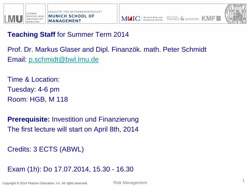
Timeline:

Date Session Content

08.04.2014 1 Introduction + Recap

15.04.2014 2 Financial Options 1

29.04.2014 3 Financial Options 2

06.05.2014 4 Option Valuation 1

13.05.2014 5 Option Valuation 2

20.05.2014 6 Tutorial 1

27.05.2014 7 Tutorial 2

03.06.2014 8 Insurance & Hedging 1

17.06.2014 9 Insurance & Hedging 2

24.06.2014 10 Tutorial 3

17.07.2014 Exam

2 Risk Management


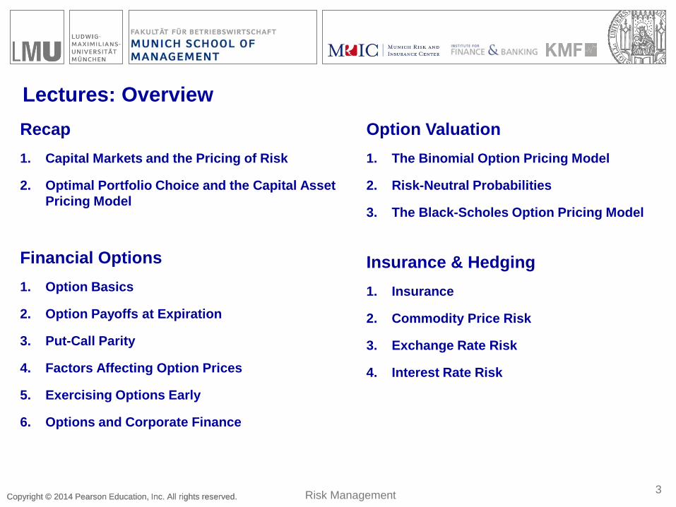
Lectures: Overview

Recap

1. Capital Markets and the Pricing of Risk

2. Optimal Portfolio Choice and the Capital Asset

Pricing Model

Financial Options

1. Option Basics

2. Option Payoffs at Expiration

3. Put-Call Parity

4. Factors Affecting Option Prices

5. Exercising Options Early

6. Options and Corporate Finance

3 Risk Management

Option Valuation

1. The Binomial Option Pricing Model

2. Risk-Neutral Probabilities

3. The Black-Scholes Option Pricing Model

Insurance & Hedging

1. Insurance

2. Commodity Price Risk

3. Exchange Rate Risk

4. Interest Rate Risk

Readings:

B & D: Chapters 10, 11, 20, 21, & 30

Copyright © 2014 Pearson Education, Inc. All rights reserved. 4

Risk Management

Copyright © 2014 Pearson Education, Inc. All rights reserved.

Common Measures of Risk and Return

• Probability Distributions

• When an investment is risky, there are different returns it may earn. Each possible return has some likelihood of occurring. This information is summarized with a probability distribution, which assigns a probability, PR , that each possible return, R , will occur.

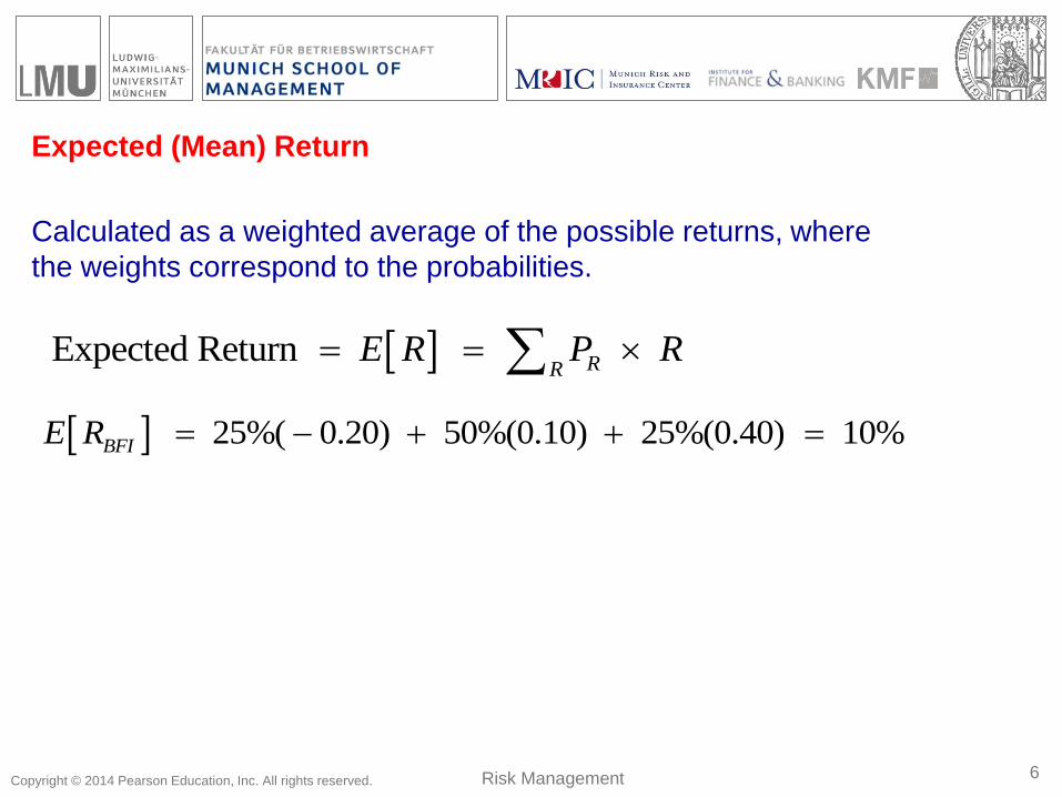
– Assume BFI stock currently trades for $100 per share. In one year, there is a 25% chance the share price will be $140, a 50% chance it will be $110, and a 25% chance it will be $80.

5 Risk Management


Expected (Mean) Return

Calculated as a weighted average of the possible returns, where

the weights correspond to the probabilities.

Expected Return RRE R P R

25%( 0.20) 50%(0.10) 25%(0.40) 10% BFIE R

6 Risk Management


Probability Distribution of Returns for BFI

7 Risk Management


Variance

• The expected squared deviation from the mean

Standard Deviation

• The square root of the variance

• Both are measures of the risk of a probability distribution

( ) ( ) SD R Var R

2 2

( ) RR

Var R E R E R P R E R

8 Risk Management


• For BFI, the variance and standard deviation are:

• In finance, the standard deviation of a return is also referred to as its volatility. The standard deviation is easier to interpret because it is in the same units as the returns themselves.

( ) ( ) 0.045 21.2% SD R Var R

2 2

2

25% ( 0.20 0.10) 50% (0.10 0.10)

25% (0.40 0.10) 0.045

BFIVar R

9 Risk Management


The Expected Return of a Portfolio

Portfolio Weights

• The fraction of the total investment in the portfolio held in each

individual investment in the portfolio

– The portfolio weights must add up to 1.00 or 100%.

• Then, the return on the portfolio, Rp , is the weighted average of the

returns on the investments in the portfolio, where the weights

correspond to portfolio weights.

10

i

Value of investment

Total value of portfolio

ix

1 1 2 2 P n n i iiR x R x R x R x R

Risk Management


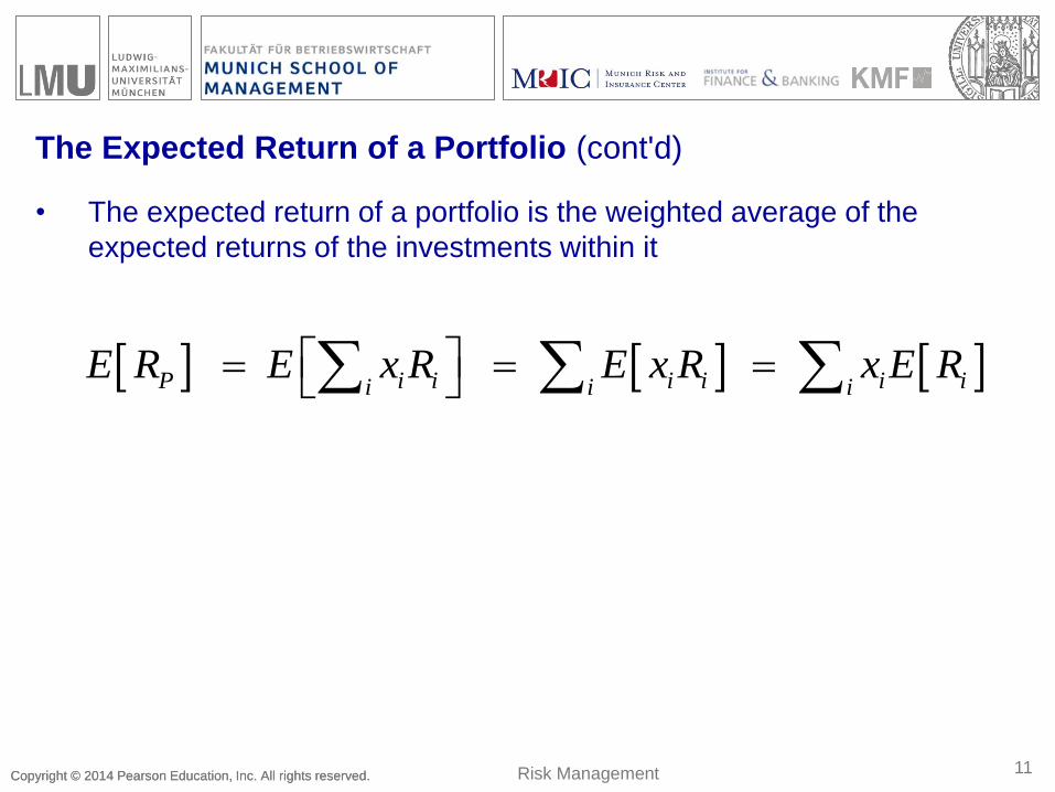
The Expected Return of a Portfolio (cont'd)

• The expected return of a portfolio is the weighted average of the

expected returns of the investments within it

11

P i i i i i ii i iE R E x R E x R x E R

Risk Management


Determining Covariance and Correlation

To find the risk of a portfolio, one must know the degree to which the

stocks’ returns move together.

Covariance

• The expected product of the deviations of two returns from their means

• Covariance between Returns Ri and Rj

• Estimate of the covariance from historical data

– If the covariance is positive, the two returns tend to move together.

– If the covariance is negative, the two returns tend to move in opposite directions.

12

( , ) [( [ ]) ( [ ])] i j i i j jCov R R E R E R R E R

, ,

1( , ) ( ) ( )

1

i j i t i j t jt

Cov R R R R R RT

Risk Management


Determining Covariance and Correlation (cont'd)

Correlation

• A measure of the common risk shared by stocks that does not depend

on their volatility

• The correlation between two stocks will always be between –1 and +1.

13

( , )( , )

( ) ( )

i j

i j

i j

Cov R RCorr R R

SD R SD R

Risk Management


Correlation

14 Risk Management


Computing a Portfolio’s Variance and Volatility

• For a two-stock portfolio:

• The variance of a two-stock portfolio

15

1 1 2 2 1 1 2 2

1 1 1 1 1 2 1 2 2 1 2 1 2 2 2 2

( ) ( , )

( , )

( , ) ( , ) ( , ) ( , )

P P PVar R Cov R R

Cov x R x R x R x R

x x Cov R R x x Cov R R x x Cov R R x x Cov R R

2 2

1 1 2 2 1 2 1 2( ) ( ) ( ) 2 ( , ) PVar R x Var R x Var R x x Cov R R

Risk Management


Risk Versus Return: Choosing an Efficient Portfolio

Efficient Portfolios with Two Stocks

• Consider a portfolio of Intel and Coca-Cola

• Assume these two stocks are uncorrelated

16

Stock Expected Return Volatility

Intel 26% 50%

Coca-Cola 6% 25%

Risk Management


Risk Versus Return: Choosing an Efficient Portfolio (cont'd)

Efficient Portfolios with Two Stocks (e.g. Intel and Coca-Cola)

17

Expected Returns and Volatility for Different Portfolios of Two Stocks

Risk Management

Calculation:

𝐸 𝑅40,60 = 0.40 ∗ 0.26 + 0.60 ∗ 0.06 = 0.14 = 14%.

𝑉𝑎𝑟 𝑅40,60 = 0.40² ∗ 0.502 + 0.60² ∗ 0.252 + 2 ∗ 0.40 ∗ 0.60 ∗ 0 ∗ 0.50 ∗ 0.25 = 0.0625 = 6.25%.

𝑆𝐴 𝑅40,60 = 𝑉𝑎𝑟 𝑅40,60 = 0.25 = 25%.


Volatility Versus Expected Return for Portfolios of Intel and

Coca-Cola Stock

18 Risk Management




• Consider investing 100% in Coca-Cola stock. As shown in on the

previous slide, other portfolios—such as the portfolio with 20% in

Intel stock and 80% in Coca-Cola stock—make the investor better

off in two ways: It has a higher expected return, and it has lower

volatility. As a result, investing solely in Coca-Cola stock is

inefficient.

19 Risk Management




• Identifying Inefficient Portfolios

– In an inefficient portfolio, it is possible to find another portfolio

that is better in terms of both expected return and volatility.

• Identifying Efficient Portfolios

– In an efficient portfolio, there is no way to reduce the volatility of

the portfolio without lowering its expected return.

20 Risk Management


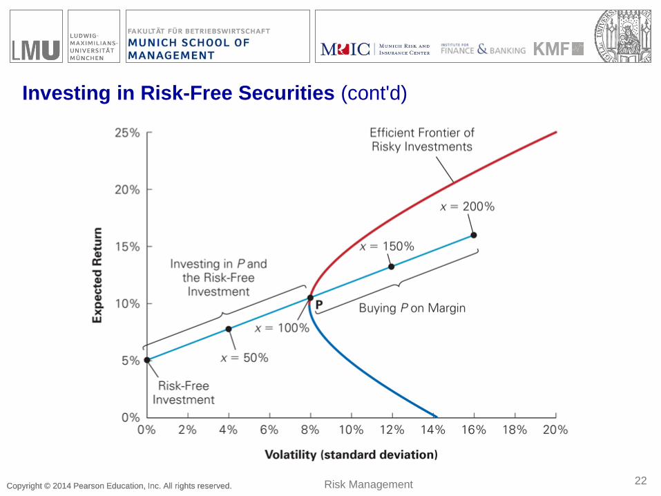
Investing in Risk-Free Securities

Consider an arbitrary risky portfolio and the effect on risk and return of putting a fraction of the money in the portfolio, while leaving the remaining fraction in risk-free Treasury bills.

• The expected return would be:

21

[ ] (1 ) [ ]

( [ ] )

xP f P

f P f

E R x r xE R

r x E R r

risk premium

Risk Management

Copyright © 2014 Pearson Education, Inc. All rights reserved. Copyright © 2014 Pearson Education, Inc. All rights reserved. 22

Investing in Risk-Free Securities (cont'd)

Risk Management


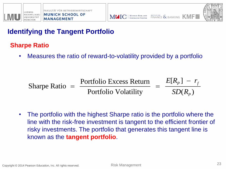
Identifying the Tangent Portfolio

Sharpe Ratio

• Measures the ratio of reward-to-volatility provided by a portfolio

• The portfolio with the highest Sharpe ratio is the portfolio where the

line with the risk-free investment is tangent to the efficient frontier of

risky investments. The portfolio that generates this tangent line is

known as the tangent portfolio.

23

[ ] Portfolio Excess ReturnSharpe Ratio

Portfolio Volatility ( )

P f

P

E R r

SD R

Risk Management


The Tangent or Efficient Portfolio

24 Risk Management


The Capital Asset Pricing Model

• The Capital Asset Pricing Model (CAPM) allows us to identify the

efficient portfolio of risky assets without having any knowledge of the

expected return of each security.

• Instead, the CAPM uses the optimal choices investors make to identify

the efficient portfolio as the market portfolio, the portfolio of all stocks

and securities in the market.

25 Risk Management


The CAPM Assumptions (3 Main Assumptions)

• Assumption 1

– Investors can buy and sell all securities at competitive market prices (without

incurring taxes or transactions costs) and can borrow and lend at the risk-free

interest rate.

• Assumption 2

– Investors hold only efficient portfolios of traded securities—portfolios that yield the

maximum expected return for a given level of volatility.

• Assumption 3

– Investors have homogeneous expectations regarding the volatilities,

correlations, and expected returns of securities.

– Homogeneous Expectations

- All investors have the same estimates concerning future investments and

returns.

26 Risk Management


Optimal Investing: The Capital Market Line

• When the CAPM assumptions hold, an optimal portfolio is a

combination of the risk-free investment and the market portfolio.

• When the tangent line goes through the market portfolio, it is called the

capital market line (CML).

27 Risk Management


The Capital Market Line

28 Risk Management


Market Risk and Beta

• Given an efficient market portfolio, the expected return of an investment is:

• The beta is defined as:

29

Risk premium for security

[ ] ( [ ] ) Mkt

i i f i Mkt f

i

E R r r E R r

Volatility of that is common with the market

i

( ) ( , ) ( , )

( ) ( )

i

Mkt i i Mkt i Mkti

Mkt Mkt

SD R Corr R R Cov R R

SD R Var R

Risk Management

(CAPM)


The Security Market Line

• There is a linear relationship between a stock’s beta and its expected

return (See figure on next slide). The security market line (SML) is

graphed as the line through the risk-free investment and the market.

30 Risk Management


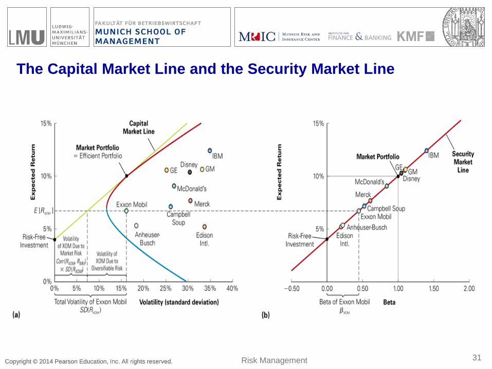
The Capital Market Line and the Security Market Line

31 Risk Management


The Capital Market Line and the Security Market Line, Panel (a)

32

(a) The CML

depicts portfolios

combining the risk-

free investment

and the efficient

portfolio, and

shows the highest

expected return

that we can attain

for each level of

volatility. According

to the CAPM, the

market portfolio is

on the CML and all

other stocks and

portfolios contain

diversifiable risk

and lie to the right

of the CML.

Risk Management


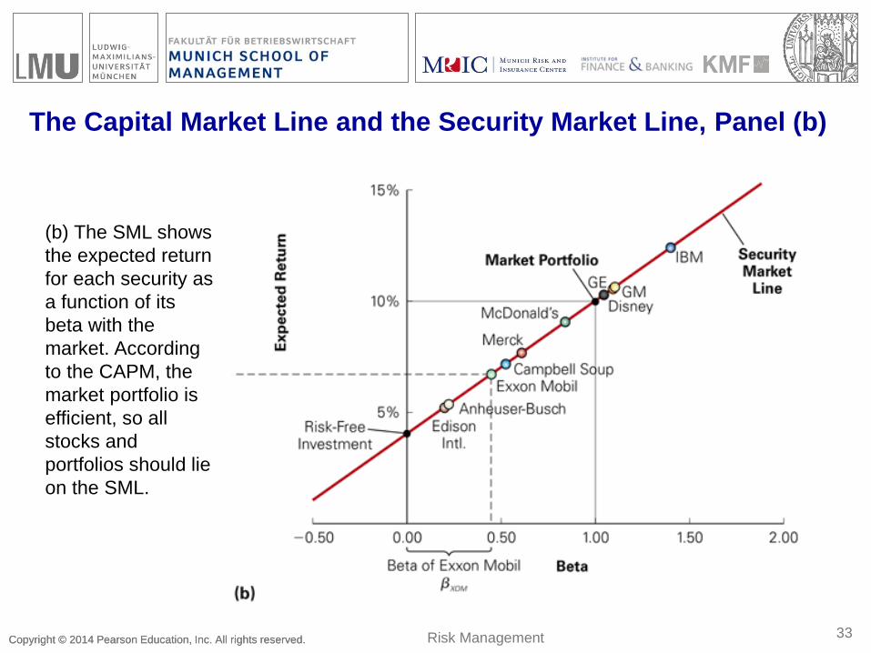
The Capital Market Line and the Security Market Line, Panel (b)

33

(b) The SML shows

the expected return

for each security as

a function of its

beta with the

market. According

to the CAPM, the

market portfolio is

efficient, so all

stocks and

portfolios should lie

on the SML.

Risk Management


The Security Market Line (cont'd)

The expected return of a portfolio

Beta of a portfolio

• The beta of a portfolio is the weighted average beta of the securities

in the portfolio.

34

, ( , ) ( , )

( ) ( ) ( )

i i MktiP Mkt i MktP i i ii i

Mkt Mkt Mkt

Cov x R RCov R R Cov R Rx x

Var R Var R Var R

)][(][ fMktPfP rRErRE

Risk Management


Example

• Suppose the stock of the 3M Company (MMM) has a beta of 0.69

and the beta of Hewlett-Packard Co. (HPQ) stock is 1.77.

• Assume the risk-free interest rate is 5% and the expected return of

the market portfolio is 12%.

• What is the expected return of a portfolio of 40% of 3M stock

and 60% Hewlett-Packard stock, according to the CAPM?

Solution

35 Risk Management


Summary of the Capital Asset Pricing Model

• The market portfolio is the efficient portfolio.

• The risk premium for any security i is proportional to its beta with the

market.

36

)][(][ fMktifi rRErRE

Risk Management


Attachment: Example

• Solution

back

37

(.40)(0.69) (.60)(1.77) 1.338 P i iix

)][(][ fMktPfP rRErRE

14.0)05.012.0(338.105.0][ PRE

Risk Management

01 Introduction Recap

Documents

risk management copyright

pearson education

pricing of risk

recap copyright

rrvar r e r e r p r

rate risk readings

common measures of risk

exchange rate risk