Gljf of Cacmrz Exped:icn Contnbution Number 3 ~0 XBT and XSV Data from the Gulf of Cadiz Expedition: R!V Oceanus Cruise 202 by -. :. - Maureen A. Kenne,y . . -. Mar, D. Prater Thomas B. Sanford CV) I 4.. . . .. . . . .. . . . . -. . P Technical Report - <-.. APL-UW TR 8920, .; 7 August 198 ' I \I SContract NO0014-87-K-0004 R9 17 09.

Welcome message from author
This document is posted to help you gain knowledge. Please leave a comment to let me know what you think about it! Share it to your friends and learn new things together.
Transcript

Gljf of Cacmrz Exped:icnContnbution Number 3
~0
XBT and XSV Data from the Gulf of Cadiz Expedition:R!V Oceanus Cruise 202
by-. :. - Maureen A. Kenne,y .. -.
Mar, D. PraterThomas B. Sanford
CV)I 4. . . . .. . . . .. . . . . -. .
P Technical Report
- <-.. APL-UW TR 8920, .;
7 August 198
' I \I
SContract NO0014-87-K-0004
R9 17 09.

Gulf of Cadiz ExpeditionContribution Number 3
XBT and XSV Data from the Gulf of Cadiz Expedition:R/V Oceanus Cruise 202
by
Maureen A. KennellyMark D. Prater
Thomas B. Sanford
Technical ReportAPL-UW TR 8920
August 1989
OCT1 7 O n
Applied Physics Laboratory University of Washington
Seattle, Washington 98105-6698
Contract NO0014-87-K-0004

UNIVERSITY CF WASHINGTON • APPLIED PHYSICS LABORATORY
Acknowledgments
We thank Paul Stevens of the Fleet Numerical Oceanography Center
for providing the T-6 XBTs. Larry Armi suggested using simultaneously
dropped XBT and XSV probes to determine salinity and shared his experi-
ence with us. John Dunlap (APL-UW) developed much of the fall rate
calculation software. This work was funded by the Office of Naval
Research under Contract Number N00014-87-K0004.

UNIVERSITY OF WASHINGTON • APPLIED PHYSICS LABORATORY
ABSTRACT
Temperature profiles from expendable bathythermographs (XBTs) and sound speed
profiles from expendable sound velocimeters (XSVs) were obtained during leg 1 of the
Gulf of Cadiz Expedition, 4-19 September 1988, from R/V Oceanus. XBTs and XSVs
were deployed around Ampere Seamount and Cape St. Vincent, Portugal. Salinity
profiles have been calculated from simultaneously dropped pairs of XBTs and XSVs.
This report describes the instrumentation used, discusses data acquisition and processing
methods, and presents temperature, sound speed, and salinity profiles.
Accession For
NTIS CP:,&IDTiC T',
By / "
Avoil biDlty CodesA-,-il and/oi' "
Dist Special
TR 8920 iii
-UNIVERSITY OF WASHINGTON -APPLIED PHYSICS LABORATORY
TABLE OF CONTENTS
Page
1.Introduction...................................................................... 1
2. Instrumentation ............................................................... 13
2.1 XBTs................................................... .............. 13
2.2 XSVs.................................................................. 13
3. Data, Acquisition............................................................... 15
4. At-Sea Data Processing.......I................................................ 17
4.1 XBT................................................................... 17
4.2 XSV ...................................................... ....... _. 174.3 Calculation of Salinity ............................................... 17
5. Post-Cruise Data Processing.................................................. 18
5.1 Calibrations .......................................................... 18
5.2 Final XBT Processing ................................................ 23
5.3 Final XSV Processing............................................... 24
5.4 Final Salinity Calculations.......................................... 24
6. Data Presentation ................................................... .......... 28j
6.1 XBT................................................................... 28
6.2 XSV................................................................... 29
6.3 Salinity ............................................................... 29I7. References...................................................................... 30
Appendix A, Oceanus Cruise 202, XBT Log ............................. Al-A8
Appendix B, Oceanus Cruise 202, XSV Log.............................. B1-B3
Appendix C, Profiles of Temperature versus Pressure ................ Cl-C113
Appendix D, P;-ofiles of Sound Speed versus Pressure................. D1-D25
Appendix E, Profiles of Temperature, Sound Speed, and Salinity.... El-E22
Appendix F, Algorithm for Computing Salinity from Temperature,Sound Speed, and Pressure.................................. FI-F3
iv R82

UNIVERSITY OF WASHINGTO '• APPLIED PHYSICS LABORATORY
LIST OF FIGURESPage
Figure 1. Operational areas for R/V Oceanus Cruise 202, Legs IV and V ............. 2
Figure 2. Survey pattern for Meddy component ....................................................... 3Figure 3. Test station locations ................................................................................. 4Figure 4. XCP survey patterns and locations of XBT drops, CTD stations,
and initial drifter deployments for the Ampere Seamount component ..... 5
Figure 5. Location of XBT drops during Meddy component .................................... 6
Figure 6. Location of XBT drops en route to Meddy and box pattern ...................... 7
Figure 7. Location of XBT drops in Meddy ........................ . ................................ . 8
Figure 8. Location of XSV drops during Meddy component ....................... ............. 9
Figure 9. Location of XSV drops during box pattern ........................................ 10
Figure 10. Location of XSV drops in Meddy .................................................... 11
Figure 11. XCP/XBT/XSV acquisition system configuration ..................................... 16
Figure 12. Relation between pressure and depth derived from thevertical integration of CTD data ................................. 19
Figure 13. Output of program comparing an XSV/XBT drop pair ............................. 21
LIST OF TABLES
Page
Table I. X SV depth coefficients ......................................................................... . 23
Table II. Sensitivity of Chen and Millero inversion ............................................ 25
Table III. Sensitivity of standard salinity computation ..................... 26
Table IV. Summary of salinity obtained from XSV/XBT drop pairs .................... 27
Table V. XBT drops for which there are no temperature profiles ....................... 28
Table VI. XSV drops for which there are no sound speed profiles ........................ 29
TR 8920 v

UNIVERSITY OF WASHINGTON • APPLIED PHYSICS LABORATORY
1. INTRODUCTION
This report is the reference volume and data summary for expendable bathythermo-
graph (XBT) and expendable sound velocimeter (XSV) data obtained during our leg 1 of
R/V Oceanus Cruise 202, the Gulf of Cadiz Expedition, 4-19 September 1988. In addi-
tion, salinity profiles derived from simultaneously dropped pairs of XBTs and XSVs are
presented.
The objectives of this expedition were to observe the vortices shed in the wake of
Ampere Seamount, to survey eddies (Meddies) formed by the Mediterranean outflow
near Cape St. Vincent, Portugal. and to study the structure and dynamics of the outflow
plume west of the Strait of Gibraltar. The cruise consisted of two legs: our leg 1, from
4-19 September 1988, corresponded to Leg IV of Oceanus voyage 202; our leg 2, from
21-28 September 1988, corresponded to Leg V. XBTs and XSVs were deployed only on
leg 1. In addition to XBTs and XSVs, expendable current profilers (XCPs) and expend-
able dissipation profilers (XDPs) were deployed, and "L stations v, ere taken uuin-g the
cruise. During the Ampere Seamount component of the expedition, a radar transponder
was moored, and four drifting buoys were tracked. The Gulf of Cadiz Expedition is
described in detail by Kennelly et al., 1989a, and the CTD data are presented by Ken-
nelly et al., 1989b.
The operational areas for the expedition included Ampere Seamount, the arca
around Cape St. Vincent, Portugal, and the Gulf of Cadiz west of the Strait of Gibraltar
(Figure 1). The sampling pattern executed in the Meddy survey region, approximately
delineated by the box in Figure 1, is shown in Figure 2. No XBT or XSV measurements
were made along sections A-I.
The XBT drop locations are shown in Figures 3-7. The XSV drop locations are
shown in Figures 8-10. XBTs 1 and 2 were test drops made shortly after leaving Fun-
chal, Madeira (Figure 3). XBTs 3 through 27 were taken during the Ampere Seamount
component of the experiment. After the radar transponder was moored on top of the
seamount and CTD station 2 was taken, the ship headed to a point 23 n.mi. northeast of
the mooring. Starting at this point, XBT sections were taken in a box pattern 60 km on a
side around the seamount (Figure 4). Probes were deployed every half hour (10 kin)
around the circuit. No XSVs were deployed during the Ampere Seamount component of
the expedition.
TR 8920 1

_______________UNIVERSITY OF WASHINGTON APPLIED PHYSICS LABORATORY
ccn
k0.0
CL~
400e0 U4 Xv Iloos 0
0 a~aniLLVI
2 TR 8920I

___________ -UNIVERSITY OF WASHINGTON APPLIED PHY ICS LABORATORY
38 NI
30' [ 1PORTUGAL
8 17
tw 370
30'0
360
30' 100 W 30' go 30' 80LONGITUDE
Figure 2. Survey pattern for Meddy component.
TR 8920 3

UNIVERSITY OF WASHINGTON APPLIED PHYSICS LABORATORY
367N I
350 AmpereSeamount
0-o
:= 340-J
CTD 10 XBT 1
330 Madeira XBT2
320 I I I180W 170 160 150 140 130 120
Longitude
Figure 3. Test station locations.
4 TR 8920

_______________UNIVERSITY OF WASHINGTON APPLIED PHYSICS LABORATORY
4 0,
30-627&
20 -&0326,a
10
~-0 100 mooring an
-10xcP
survey 2 23A
-20J
& 15 16 400D0M
-30 - & 7 &B 18 l9 A20
9 CTD a XBT T7 + drifter
-40 -30 -20 -10 0 10 20 30 40x (kin)
Figure 4. XCP survey patterns and locations of XBT drops, CTD stations, and initialdrifter deployments for Ampere Seamount component. Crude topography isalso shown.
TR 8920 5

-UNIVERSITY OF WASHINGTON APPLIED PHYSICS LABORATORY
38- N
182.183
181
*180179
301030' 17:0 PORTUGAL
1177
0176174
0175
161 162 163 166 167 168 169 170 1'71 172
37~ 164,165
160 159 158 157 156 15,5 154 153 1 49515 . . .4
00t 0 066
1040 & 82 A6£38
13 4114 8' 84-,37 139 140 143 144 145 __46 14&4805£ 6
138 141,142 0 043 103102 4
136 135 134 133 132 131 130 129 12 5 *Be08 080 062 04 036
128.7127 125 100_878
106 100 089-1-/ 061 512 9 0 7 0 4 3
117 118 119 120 121 122123 107 99#0 *q9 76
*33116 094705 040 980 09 05 58
115114 113 112 111 110 1 :5 484 032*0 0 0 0 970 *92 94 It 19 3
960 093 * o 5- ) 029
1090 0 0972 54 .05236 0 9 069 02*36C T 201-229 95 71 5
* XBT T6 070* XBT T7
30' 100 W 30' 90 30' 80LONGITUDE
Figure S. Location of XBT drops during Meddy component. Drops during survey ofMeddy (201-229, boxed area) are shown in detail in Figure 7.
6 TR 8920

UNIVERSITY OF WASHINGTON APPLIED PHYSICS LABORATORY
30'PORTUGAL
018
30' *8
199 193 .90 0009 0197
20036'- 194o *19 0196
*XBT T5
30' l1o W 30' go 30' 8'LONGITUDE
Figure 6. Location of XBT drops en route to Meddy and box pattern.
TR 8920 7

UNIVERSITY OF WASHINGTON APPLIED PHYSICS LABORATORY
36025'N
20'
15' -
0210
@20910' - 221
a @222 2211I- 223 0207
2240 206 02125' -2256 -14 213
215 OP 12052169 0226
2179 0204 0227
2189 *228219. 0203 0229
36000' - 2200 1
0202
0201
55'-
*XBT T5
50' I I I I 1
9030'W 25' 20' 15' 10' 5' 9o00 55,LONGITUDE
Figure 7. Location of XBT drops in Meddy.
8 TR 8920

_______________UNIVERSITY OF WASHINGTON APPLIED PHYSICS LABORATORY
38- NS Ek -
019
30'PORTUGAL
*18
00
- 1
30'9
*13
414
36'28-55
*XSV 020 XSV 03
30' 100 W 30' 90 30' 80LONGITUDE
Figure 8. Location of XSV drops during Meddy component. Drops during survey ofMeddy (28-55, boxed area) are shown in detail in Figure 10.
TR 8920 9

UNIVERSITY OF WASHINGTON APPLIED PHYSICS LABORATORY
38, N
PORTUGAL
*~370
30'
. 2736-
21 22 23
*XSVO02
30' 100 W 30' 90 30' 8
LONGITUDE
Figure 9. Location of XSV drops during box pattern.
10 MR8920

UNIVERSITY OF WASHINGTON APPLIED PHYSICS LABORATORY-.
3625'N I
20'
15'
*37
*3610' -47w *48 *38
I.- *49 *34
< #50 33 •39
" 51e *A4042# 32
#43 *31 *53
*44 54**45 *3055
36 00' -46*29
*28
55'-
*XSV 02
50' I I 1
9030'W 25'J 20' 15' 10' 5' 9°00 ' 55'LONGITUDE
Figure 10. Location of XSV drops in Meddy.
TR 8920 11

UNIVERSITY OF WASHINGTON • APPLIED PHYSICS LABORATORY
XBTs and XSVs were deployed near Cape St. Vincent, Portugal, along the lines of
the Meddy survey pattern (Figure 2). XBTs were dropped along all lines of the pattern
(Figure 5), whereas XSVs were deployed only along lines 2, 3, 4, 8, 13, 14, 15, 17, and
19 (Figure 8). Problems were encountered with the XSVs during the early deployments.
They would not process or display. By XSV drop 12, however, the problem had been
identified as a manufacturing error. Many of the probes were misaligned, with the result
that correct electrical contact was made by the launcher pins only 1/3 of the time. Subse-
quently, the probe alignment was checked, and if necessary the probes were realigned
before launch.
After the Meddy survey pattern was completed and the data were reviewed, it was
decided to study a Meddy that had been identified near CTD 25 (36°10.15'N, 9"02.1'W).
En route to that position, XBTs were taken hourly starting with the crossing of line 14,
with half hourly drops after crossing line 12 (Figure 6, XBTs 185-190). Little evidence
of the 12'C core seen in CTD 25 was found on the way, so a box pattern survey (XBTs
191-200) was commenced. XSVs were also dropped during the box survey (Figure 9,
XSVs 20-27). Finally, the Meddy was found about 10 n.mi. SW of CTD 25. A star pat-
tern was then commenced to survey the Meddy using XCPs, XBTs (Figure 7), and XSVs
(Figure 10).
No XBTs or XSVs were deployed on the second leg of the Gulf of Cadiz Expedi-
tion. Instead, the CTD profiler was used on all stations.
12 TR 8920

UNIVERSITY OF WASHINGTON • APPLIED PHYSICS LABORATORY
2. INSTRUMENTATION
2.1 XBTs
Three types of Sippican Inc. XBTs (T-5, T-6, and T-7), going to depths of 1830 m,
460 m, and 760 m respectively, were used during the cruise. Hand-held launchers
inserted into deck-mounted launch tubes were located on both the starboard and port aft
quarters of the ship. Each launcher was electrically tested for line resistance and isola-
tion. The launcher initially provided by the ship failed these tests and was replaced with
a new launcher. Each launcher was connected to a MK-9 receiver. In all, 229 XBTs
were deployed. Appendix A gives the drop particulars.
Seven type T-6 probes were deployed during the cruise, and all provided good data.
Forty T-7s were deployed, with a 90% success rate: two did not provide good data, and
two did not provide data to full depth. The T-5 success rate was somewhat
disappointing-82%, or 150 good drops out of 182. The failure modes were as follows:
13 yielded no good data, 13 did not provide data to full depth, 3 had obvious temperature
offsets, 2 were noisy, and 1 contained temperature jumps.
2.2 XSVs
Two types of Sippican Inc. XSVs (XSV-02 and XSV-03), going to depths of
2000 m and 850 m respectively, were used during the cruise. The same launchers and
MK-9 receivers (with the addition of XSV boards) were used for the XSVs as for the
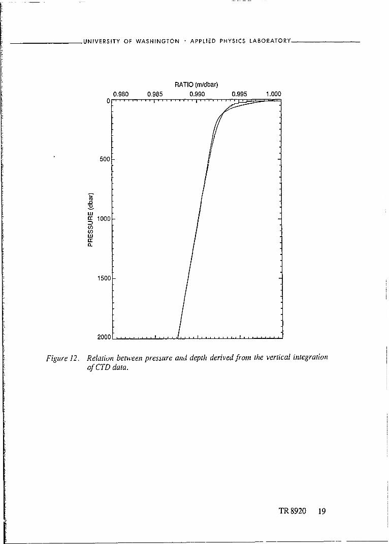
XBTs. In all, 55 XSVs were deployed. Appendix B gives the drop particulars.
During the first few deployments, the XSVs would not process or display. When an
XSV-02 (slowfall type) was launched, it neither started the MK-9 nor provided ac signals
more than 10 mV. Better electrical grounds were placed on the MK-9; however, the new
grounds did not seem to solve the problem. Next, the XSV boards were swapped
between MK-9 units. The next XSV-02 (XSV 5) worked well, giving voltages of more
than a volt.
However, the XSV failure problem recurred. Seldom were the proper prelaunch
voltages measured from the MK-9 or usable signals received from the falling probes.
The condition of the launcher and cables was repeatedly checked. For a while it was
thought one or both of the XSV boards were damaged.
TR 8920 13

UNIVERSITY OF WASHINGTON APPLIED PHYSICS LABORATORY
Closer examination of the XSVs revealed that the cannister was often improperly
aligned with the shipboard spool. Evidently, the probes were assembled without regardto the notch on the cannister and the arrowhead on the spool. There are three connecting
tabs on the cannister, allowing three different orientations between the cannister and
spool. Because only one orientation permits the correct connections to be made at the
launcher, the data return was poor. Seven probes failed before our discovery of the
manufacturing error. The remaining probes were checked and realigned if necessary.
The probes that were realigned are noted in Appendix B.
Of the 55 XSVs launched, 52 were type 02 and the remaining three were type 03.
All the type 03s provided good data. The overall success rate for the type 02s was 79%.
Before the manufacturing error was detected, seven of the first nine XSV-02s failed.
After that, one failed to provide good data, another was noisy, and two did not provide
data to full depth.
14 TR 8920

UNIVERSITY OF WASHINGTON APPLIED PHYSICS LABORATORY
3. DATA ACQUISITION
An integrated acquisition program written in HP-Basic provided the acquisition of
XCP, XBT, and XSV data in real time with a Hewlett Packard HP9020 computer. In this
report only the XBT and XSV parts of the acquisition system will be discussed. Real-
time processing and display of the data were also provided by the program. Data from up
to three probes could be acquired and displayed simultaneously (with three co-running"partition" programs controlled by a fourth "master" program). Raw XBT and XSV data
were archived onto floppy disk. In addition, a. the data were acquired, the complete raw
data stream was saved on an HP9144 magnetic cartridge tape drive connected to theHP9020. Raw data from XBTs and XSVs were stored daong with a time stamp, an indi-cation of the probe's type, and the partition that acquired the data.
A schematic of the acquisition system is shown in Figure 11. MK-9 XBT/XSV
receivers were connected to partitions 2 and 3 on the computer via GPIB cable.
In case of computer failure, the data were also stored on VHS audio/video magnetic
tape. One backup system was dedicated to the XBT/XSV data. The backup system con-
sisted of a VCR, Sony model PCM-F1 digital audio processor (PCM stands for pulse
code modulation; use of the PCM processor allowed us to record the two audio channels
of XSV data on the video tracks of a VHS tape), and power adapter. The XBT and XSV
data were sent to the backup system as four frequency-modulated signals. The XSV sig-
nals are FM signals to begin with. They needed only to be amplified and filtered to be
recorded. The XSV data were passed through a digital audio processor and stored on the
video tracks of a VHS tape. The XBT output was an analog voltage that was converted
to an FM signal. The frequency range of the XBT FM signal was selected to use the fre-
quency range of the air deployed XBT (AXBT), so that with a little work the AXBT card
in the MK-9 receiver could be used to play through the backup data if needed (the stan-
dard AXBT output is an FM signal). The converted FM XBT data were stored on the
two VHS audio tracks. Both MK-9s were modified to produce frequency-modulated vol-
tages for recording the XBT data on VHS tape.
i
I~TR 8920 15

4 Element Y'agi7 Verticallyj PolarizedAntennaFacing Aft
2-watjSplitter
Processor ----
AUDIO
'0MI' DiskXCP sgnal230 KB~te Floppy
SpitrProcessor Slot 2 Color Graphics CRTAUDIO GPIB Thermal Printer
2. .yt RAM
PoesrSo Adpe4o~ ui iia
AUDIO
H I Raiicu
and Pilot @ot 05aaoi H
16 16RM-1020I

UNIVERSITY OF WASHINGTON - APPLIED PHYSICS LABORATORY
4. AT-SEA DATA PROCESSING
4.1 XBT
The acquisition program provided a printout of the isotherm depths as the probe was
falling. Hand-contoured sections of isotherms were then produced. Waterfall plots of the
temperature profiles overlaid on computer-generated isotherm sections were produced
while the acquisition program was paused. To obtain a graph of an individual XBT tem-
perature profile, the floppy disk with the XBT raw data was removed from the HP9020running HP-Basic (the acquisition computer) and transferred to the HP9020 running
UNIX. The data were loaded onto the HP9020 UNIX, a decoding program written by
John Dunlap was run on the data, and a profile was generated.
4.2 XSV
Individual sound speed profiles were obtained in the same manner as for the XBTs.
When an XSV was compared with a simultaneously dropped XBT, it was noticed that
features did not line up in depth exactly. Visual inspection of the XSV profiles showed
ocean features to be 8% shallower than in comparable XBT profiles. The XBT depthsweie believed to be accurate based on the work of other investigators (Heinmiller et al.,
1983; Seaver and Kuleshov, 1982). This was our first indication that the XSV fall rate
might be significantly incorrect.
4.3 Calculation of Salinity
Once the data had been loaded into the HP9020 UNIX computer and decoded, salin-ity was calculated from simultaneously dropped XBTs and XSVs using a program writ-
ten by John Dunlap. This program read both profiles, temperature and sound speed,
interpolated each onto an equally spaced depth grid, and shifted the XSV profile to max-
imize its correlation with the XBT profile. Salinity was calculated based on an inversion
of the Del Grosso (1974) sound speed equations. A more detailed discussion of a varia-
tion of this program is given in Sections 5.1 and 5.4.
TR 8920 17

UNIVERSITY OF WASHINGTON - APPLIED PHYSICS LABORATORY
5. POST-CRUISE DATA PROCESSING
5.1 Calibrations
To combine data from expendable probes (such as XBTs, XSVs, and XCPs) with
CTD data for contouring and computing heat and salt transports, the depth needs to be
calibrated against a standard. For the expendable probes used in this experiment, the
depth (and thus the fall rate) of the probe is estimated as a quadratic function of time.
The coefficients of the quadratic polynomial are empiricaily determined by Sippican inc.,
the manufacturer of the probes. During the Gulf of Cadiz experiment, we had an oppor-
tunity to verify the depth estimates of the probes by comparing the high-wavenumber
structure of their temperature or sound speed signal with that obtained by the Sea-Bird
CTD unit. This process also gave us information about the random errors and systematic
offsets in these variables. This section summarizes the computational procedure andpresents the results. An additional comparison was made between the XSVs and the
XBTs, since the data from these probes can be combined to estimate salinity.
Because the CTD's vertical variable is pressure and the expendable probe's variable
is depth, a conversion is needed before the expendable probe's depth can be calibrated.
Saunders and Fofonoff (1976) published a conversion method that consists of integrating
the hydrostatic equation downward from the sea surface while accounting for the hor-
izontal and vertical variations in the earth's gravitational field. For this analysis, the
CTD data collected on the cruise were averaged into 10-dbar bins, and the vertical
integration was performed for each cast. At each bin level, a ratio was formed between
the computed depth (in meters) and the measured pressure (in decibars). The resulting
ratio-pressure curves from all the casts were combined at each bin level to give a curve
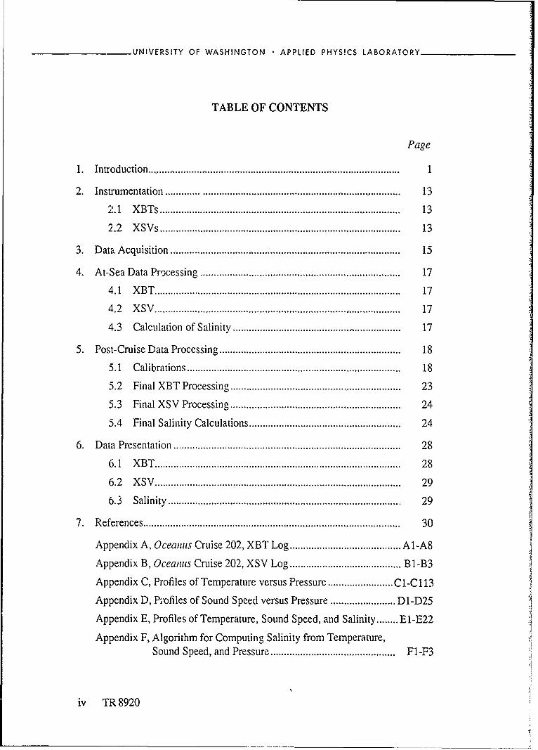
for the average ratio. An approximation to the average ratio curve is given by
ratio (pressure) = 0.9927 - 2.55 x 10⁻⁶ pressure + 0.0073 exp (-pressure/50).
Figure 12 shows the average ratio curve (steppy) and the approximate curve
(smooth). The depth is found by multip'ying the measured pressure by the ratio
appropriate for that pressure. If the pressure is 1000 dbar, for example, the correspond-
ing depth is 1000 x 0.9901, or 990.1 m. The maximum error in depth caused by using
the approximate curve instead of the one for any particular CTD cast is about 0.5 m.
18 TR 8920
I
_______________UNIVERSITY OF WASHINGTON APPLIED PHYSICS LABORATORY
RATIO (m/dbar)0.980 0.985 0.990 0.995 1.000
0C . . . .. . . .
500
co
cc 1000U)U)
1500-
20001. . . . . . .
Figure 12. Relation between pressure and dept/h derived fr-om the vertical integration
of CTD data.
TR 8920 19

UNIVERSITY OF WASHINGTON APPLIED PHYSICS LABORATORY
Pressure and depth will be used interchangeably in this section but with the understand-
ing that the appropriate conversions have been made.
Software was developed by John Dunlap and Mark Prater to determine the relative
depth offset as a function of depth between two drops or casts, assuming the instruments
passed through similar ocean features on their descent. The vertical scales of the features
used to compare the depths were between 10 and 100 m. To accent these features, the
signal from the probe (eithe- temperature or sound speed) was bandpass filtered to
remove very high wavenumber noise and low wavenumber features. The program then
shifted one profile with respect to the other and found the depth offset that maximized the
correlat'on of the two over a limited depth range. This process was repeated for each
depth value in the drop. Rather than compute the correlation for every offset possible, a"golden section search" (Press et al., 1986) was performed to find the maximum correla-
tion. The correlation was assumed to be a smoothly varying function of offset, with a
global maximum at the optimal offset. The optimized search procedure gave results
comparable to those of the point-by-point search and ran 5 to 10 times faster. The max-
imum correlation achieved and the corresponding depth offset were recorded, as well as
the temperature or sound speed differences in the nonfiltered signals at the optimum
offset. Figure 13 shows an example of the program output for an XSV/XBT drop pair.
After the depth offset record -was obtained for all the expendable probes, a second
program was used that computed the mean and rms of the depth offset and the signal
differeice. During many drops, the maximum correlation at a depth bin was below 0.5,
lowering the confidence that a good estimate of depth offset and signal difference was
obtained. To keep these values from being included in the average and contributing to
the mis, if the maximum correlation obtained for each depth bin during a drop was below
a user defined minimum (usually 0.9), the depth offset and signal difference were not
included in the subsequent calculation.
A probe/CTD pair was considered acceptable for analysis if the processed data from
the probe passed visual inspection (no noticeable offsets, spikes, wire breaks, etc.) and
the probe was dropped within I hour and within I n.mi. (2 km) of the CTD cast. These
spatial and temporal constraints may appear harsh, especially compared with a previous
error analysis by Heinmiller et al. (1983) which used XBT/CTD pairs from 15 to 50 km
apart; however, because of the complex structure and interleaving of the Meditcrranean
20 TR 8920

_______________UNIVERSITY OF WASHINGTON APPLIED PHYSICS LABORATORY
CC
C)CoE0w
E
CL
0.ucu
c
CC
Lo 1 .i.
-) >~
x E- >
E U)
a))F-0.*o0x >C
x U)
0)E~
EdN ainsSG-
TR820 2

UNIVERSITY OF WASHINGTON • APPLIED PHYSICS LABORATORY
outflow in the Gulf of Cadiz, small differences in time or position severely degraded the
signal correlations.
This analysis was carried out for all the CTD and expendable probes. In this report,
however, we will discuss only the XBT/CTD, XSV/CTD, and XBT/XSV comparisons.
Four T-5 XBT/CTD pairs, one T-6 XBT/CTD pair, and one T-7 XBT/CTD pair were
used in this analysis, but did not provide enough comparisons to estimate the depth
offsets accurately. However, a systematic mean temperature offset of 0.075'C was
observed throughout the drops, with an rms temperature variation of less than 0.1'C. The
accuracy of the probe is given by Sippican Inc. to be ±0.1 5'C.
Three XSV-02/CTD and two XSV-03/CTD pairs were used in this analysis. During
the cruise, it was noticed that features apparent in XSV data were roughly 8% shallower
than similar features observed in the XBT or CTD data. A more accurate estimate could
not be made at the time because of the small number of pairs. A better estimate of the
depth offset is made later in this section. The analysis showed a 0.20 m s- 1 offset in all
the sound speeds. The sound sensor is probably the same for all XSV probes, so the
same offset is expected for both types of XSVs. The accuracy of the probe is given by
Sippican as ±0.25 m s- .
The XSV-02/XBT(T-5) drop pairs gave the highest quality intercomparisons
because the two probes were dropped simultaneously with a spatial separation of only
10 m (the width of the fantail). XSV depths were multiplied by 1.08 before processing to
partially correct the depth offset noticed on the cruise and to reduce the search for the
maximum correlation. Table 1 gives the depth coefficients computed from this analysis
along with those given by Sippican Inc. and those used on the cruise. The depth of the
probe is given by
depth = pcalO + (pcall x t) + (pcal2 x t 2),
where t is the elapsed time in seconds since launch. The pcal's denote the coefficients of
a quadratic equation relating the time of fall and depth of the p.obe and have no unique
values without identification of the specific :,robe type. The analysis shows that the rms
error between the XSV and the XBT depth varies linearly with depth from 1 m at the sur-
face to 6 m at 1500 m.
22 TR 8920

UNIVERSITY OF WASHINGTON • APPLIED PHYSICS LABORATORY
Table I. XSV depth coefficients.
Sippican Cadiz CruiseCoefficient Sippican (1.08 x Sippican) Analysis
pcalO 0.0 0.0 3.38pcall 5.5895 6.0367 5.8561pcal2 -0.00147 -0.00159 -0.000883
This analysis assumes that the XBTs have the correct fall rate. The T-5 XBT/CTD
comparison, although limited, supports this assumption. Subtracting 0.075°C from the
T-5 XBT temperatures is recommended. There were too few comparisons with CTDs to
recommend adjusting the T-6 or T-7 temperatures. The Cadiz cruise depth coefficients
are recommended for any XSV-02 processing, along with adding 0.2 m s- 1 to the sound
speeds. Because of the limited data for XSV-03s, their depths have been assumed to be
correct; however, since they use the same sound sensor as the XSV-02s, it is recom-
mended that 0.2 m s- 1 be added to the sound speeds.
5.2 Final XBT Processing
Many probes continued to transmit data after they hit the seafloor. Others failed
before reachirg their full depth capability. It is important to exclude such bad data from
later analysis. Therefore a database was created of end-of-good-data depths. The value
for the end depth was determined by scanning the unaveraged data values and finding the
depth of the last good data point. The data were then passed to a program that accessed
the end-depth database and retained only good data. Depths were converted to pressure
using the following relation between pressure and depth determined from the Cadiz data:
ratio = 0.9927 + 2.55 x 10⁻⁶ x (XBT depth) + 0.0073 x exp (XBT depth/50)
XBT pressure = -(XBT depth/ratio).
Processing of the T-5 XBT data involved an additional step: 0.075C was subtracted
from the temperature values. Finally, the data were gridded into 2 dbar values.
TR 8920 23

UNIVERSITY OF WASHINGTON APPLIED PHYSICS LABORATORY
5.3 Final XSV Processing
A database of end-of-drop depths was also created for the XSV probes, and the
same processing scheme was employed as for the XBTs. Type 02 XSV depths were
corrected and converted to pressure in the following manner. First, we solved for time of
fall by inverting the fall rate equation to obtain
t = -pcall + "4pcal12 - 4(pcal2)(pcal0 + XSV depth)2pcal2
where the pcal's are Sippican's XSV fall rate coefficients and have the values
pcal0 = 0.0
pcall = 5.5895
pcal2 = -0.00147.
Then we computed the new depth from time.
New XSV depth = -[pcalO + (pcal I x t) + (pcal2 x t 2)],
where these pcal's are the Cadiz cruise XSV coefficients determined in Section 5.1 and
have the values
pcal0 = 3.38
pcall = 5.8561
pcal2 = -0.000883.
The "new XSV depths" were then converted to pressure in the same manner as the XBT
depths. The type 03 XSV depths were not corrected; only the conversion to pressure wasmade. The sound speeds for both the type 02s and 03s were adjusted by adding
0.2 m s- 1. The data were then gridded into 2 dbar values.
5.4 Final Salinity Calculations
A conventional CTD would have taken 90 minutes to deploy, cast to 1800 m, and
recover. To survey the Meddy rapidly, expendable temperature and sound speed probes
were used in the hope that these data could be combined to compute salinity. The poorer
data quality was more than offset by the ability to sample the feature quickly. The
24 TR 8920

UNIVERSITY OF WASHINGTON APPLIED PHYSICS LABORATORY
expendables were launched while the ship was slowed to 5 knots. This section summar-
izes the problems encountered and the method used to compute salinity.
Chen and Millero (1977) developed equations to calculate the speed of sound in
seawater as a function of temperature, salinity, and pressure. For this study, their equa-
tions have been inverted to calculate salinity as a function of sound speed, temperature,
and pressure (Appendix F). Chen and Millero's equations were chosen because their
method is the most recent, encompasses the widest range of pressures, temperatures, and
salinities, and is the UNESCO standard for computing sound speed (Fofonoff and Mil-
lard, 1983). In addition, the sound speed comparisons between the XSV and the CTD
data and the salinity comparisons between the XSV/XBT pairs and the CTD data would
then be consistent. The major problem with computing salinity with this inversion tech-
nique is that the value computed is very sensitive to changes in pressure and temperature.
The sensitivities of the Chen and Millero inversion are given in Table 2, along with the
accuracies needed to estimate salinity to within 0.1 psu. The accuracies of the XSV and
XBT probes as given by Sippican Inc. (1983) are also presented.
Table H. Sensitivity of Chen and Millero inversion.
Variable Sensitivity Accuracy Needed for 0.1 psu Accuracy of Probes
Depth -0.0138 psu/dbar 7.2 dbar 2% of depthTemperature -2.8775 psu/ 0 C 0.0350C 0. 150CSound Speed 0.8340 psu/m s- t 0.12 m s- I 0.25 m s- 1
The sound speed equation of Chen and Millero itself has an uncertainty of
0.2 m s-l. For comparison, the sensitivities of the standard salinity computation from
temperature, pressure. and conductivity are given in Table 3.
Because of the sensitivity of the Chen and Millero inversion to pressure, tempera-
ture. and sound speed, computing salinity from an expendable conductivity cell of
moderate accuracy is far better than computing it from an expendable sound speed probe
with very good accuracy. However, we will do the best with what we have.
TR 8920 25

UNIVERSITY OF WASHINGTON • APPLIED PHYSICS LABORATORY
Table III. Sensitivity of standard salinity computation.
Variable Sensitivity Accuracy Needed for 0.1 psu
Depth -0.0004 psu/dbar 250 dbarTemperature -0.9145 psu/°C 0.11 0 C
Conductivity 9.7095 psu/S m- 1 0.01 S m- 1
To minimize the depth offset between the XBT and XSV data, we used the actual
offsets found by the depth analysis for specific probe pairs instead of the depth
coefficients found in Section 5.1. A polynomial was fit to the offset data so that regions
of low correlation would be smoothed over. The depths of the XSV probes were then
corrected using the polynomial fit, and the output was gridded to 2 m (the same as the
output of the depth analysis). The salinity was then computed from the temperature,
sound speed, and pressure (which is computed from depth) and gridded again on a larger
scale (bin size 20 dbar, step size 2 dbar) for increased smoothing. At this point, we
noticed that the salinity profile computed from the XBT/XSV data often had thl same
structure as that computed from the CTD data but was offset. To correct the offset, we
comput-a the average salinity at the 300 dbar and 1600 dbar levels from the CTD data
nearest the XSV/XBT pairs. These depths were chosen because they were above and
below the effect of the Mediterranean outflow for most of the casts. The XSV/XBT
salini'ties were then corrected so that they matched the CTD average of 35.75 psu for
those two levels. The rms error in using the average salinity value at those depths is
about 0.04 psu. The salinities were regridded (bin size 50 dbar, step size 2 dbar) for the
final plots.
Overall, we were able to compute salinity fairly well from XSV and XBT data. Out
of 55 XSVs dropped, 47 returned data. Of those, five were not dropped concurrently
with a working XBT, leaving 42 usable drop pairs. Of those, 29 yielded good quality
profiles and 13 poor quality. Quality was judged subjectively, based on how well the
temperature versus salinity curves calculated for the expendable drop pairs resembled
those obtained from nearby CTD casts. Good quality XSV and XBT data occasionally
resulted in poor quality salinity values due to the extreme sensitivity of the inver,,ion
26 TR 8920

UNIVERSITY OF WASHINGTnN - APPLIED PHYSICS LABORATORY
equations to temperature and sound speed, whereby seemingly inconsequential devia-
tions in those N ariables lead to very wrong estimates of salinity. The results are summar-
ized in Table 4.
Table IV. Summary of salinity results obtained from XSV/XBT drop pairs.
XSV Data XBT Data Salinity XSV Data XBT Data SalinityNo. Quality No. Quality Quality No. Quality No. Quality Quality
1 Fail Bad 31 Good 204 Good Good2 Fail Bad 32 Fail 205 Good Bad3 Fail Bad 33 Good 206 Good Poor4 Fail Bad 34 Good 207 Poor Poor5 Good 58 Good Good 35 Good 208 Good Good6 Fail Bad 36 Good 209 Fail Bad7 Fail Bad 37 Good 210 Good Good8 Good Bad 38 Good 211 Good Good9 Good Bad 39 Poor 212 Good Poor
10 Fail Bad 40 Good 213 Good Good11 Good 105 Good Poor 41 Good 215 Fail Bad12 Good 106 Poor Poor 42 Good 216 Poor Poor13 Good 107 Good Good 43 Good 217 Good Good14 Good 108 Good Good 44 Good 218 Good Good15 Good Bad 45 Good 219 Good Good16 Good 148 Good Poor 46 Good 220 Poor Poor17 Good 155 Good Good 47 Good 221 Good Poor18 Good 174 Good Poor 48 Good 222 Good Good19 Good 184 Good Good 49 Good 223 Good Good20 Good 193 Good Good 50 Good 224 Good Good21 Good 194 Good Good 51 Good 225 Good Good22 Good 195 Good Good 52 Good 226 Poor Poor23 Good 196 Good Good 53 Good 227 Poor Poor24 Good 197 Good Good 54 Good 228 Good Good25 Good 198 Good Good 55 Good 229 Good Poor26 Good 199 Good Good27 Good 200 Good Good28 Good 201 Good Good29 Good 202 Good Good30 Good 203 Good Good
TR 8920 27

UNIVERSITY OF WASHINGTON • APPLIED PHYSICS LABORATORY
6. DATA PRESENTATION
6.1 XBT
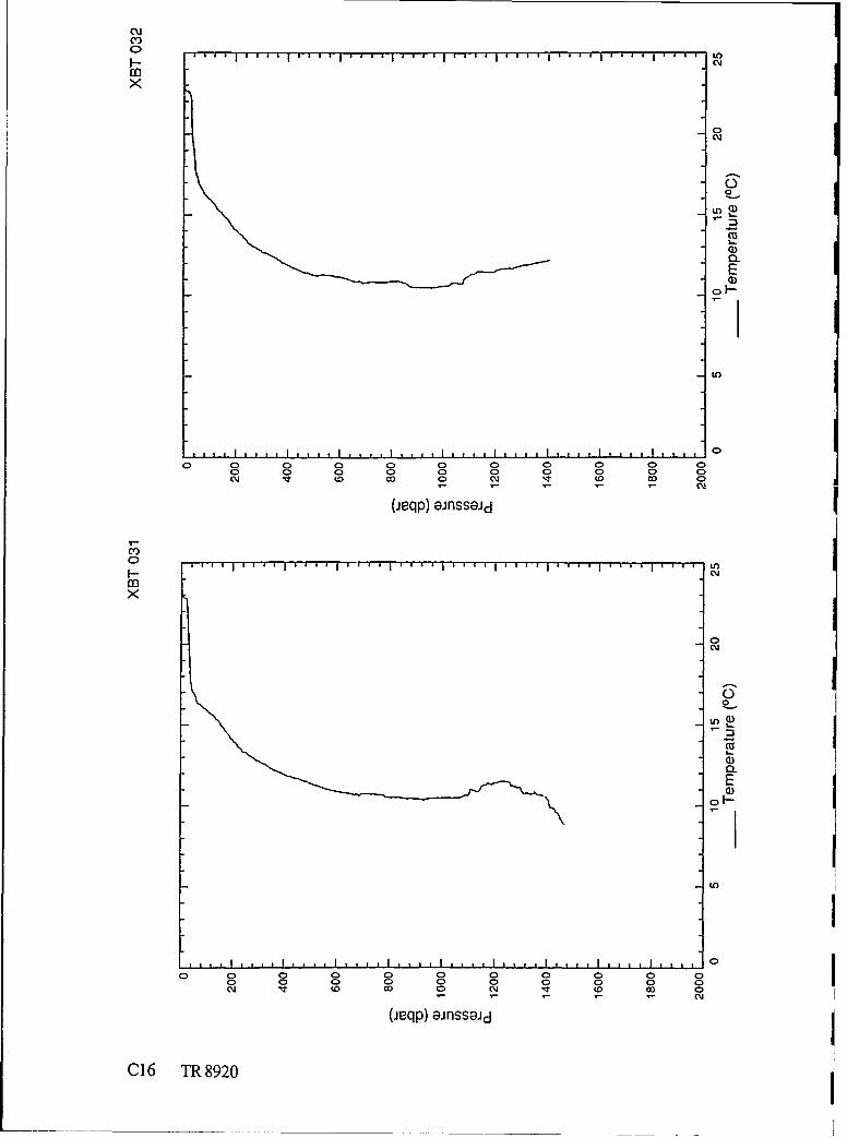
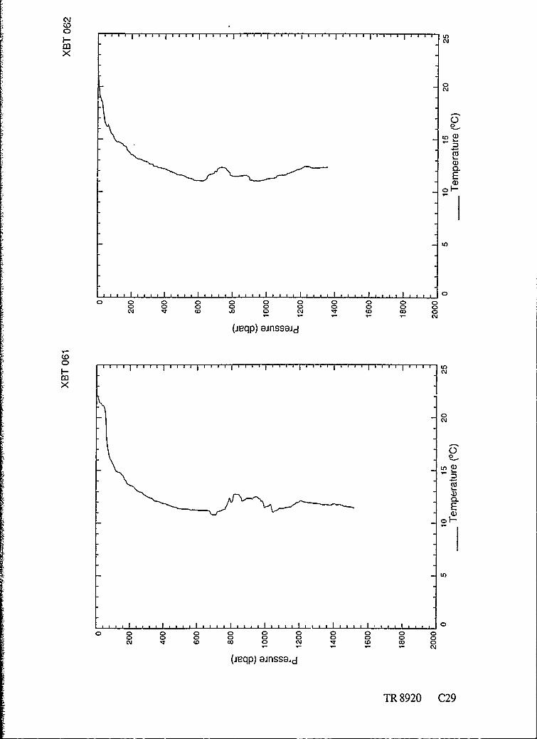
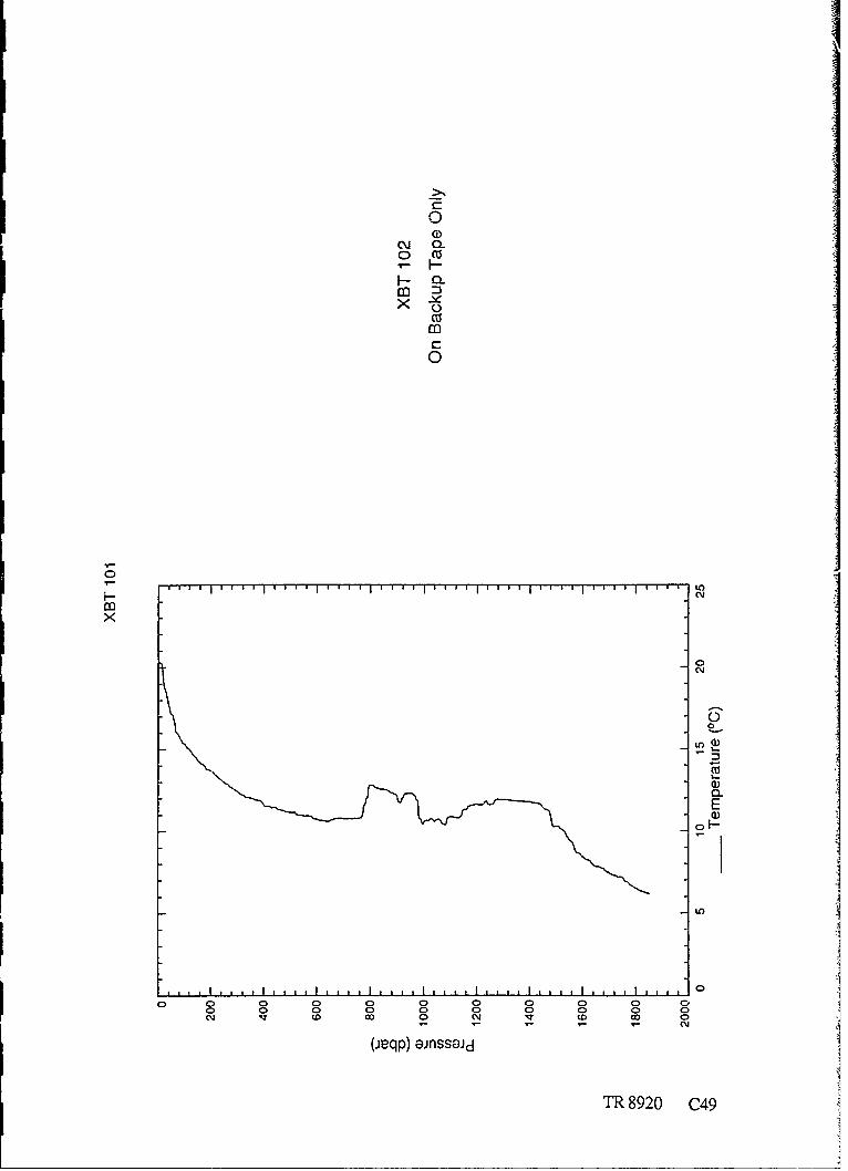
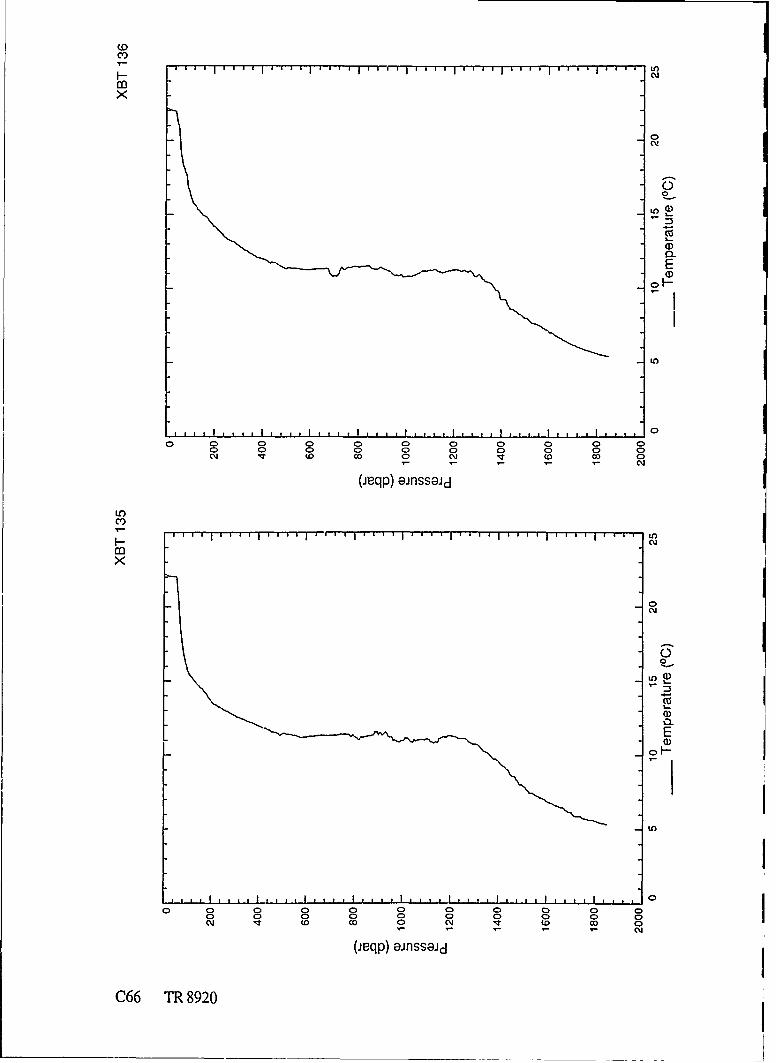
Profiles of temperature versus pressure calculated from the XBT data (2 dbar aver-
ages) are presented in Appendix C. Drops for which no data are presented are listed in
Table 5 with explanatory comments. All data that were not obviously bad are included in
the appendix. Some data in Appendix C may be of questionable quality. At this prelim-
inary stage of the analysis, however, we do not wish to throw out data that we may be
able to correct at a later time.
Table V. XBT drops for which there are no temperature profiles.
XBT Comment
45 On backup tape only; needs to be played back53 No file created54 Bad55 On backup tape only; needs to be played back:)6 Bad57 Off scale59 Bad67 Bad83 Off scale87 Off scale
102 On backup tape only; needs to be played back141 Off scale150 Bad182 Bad183 Bad205 Bad209 Bad214 Bad215 Off scale
28 TR 8920

UNIVERSITY OF WASHINGTON APPLIED PHYSICS LABORATORY
6.2 XSV
Profiles of sound speed versus pressure calculated from the XSV data (2 dbar aver-
ages) are presented in Appendix D. Profiles are shown for all good XSV drops. The
same depth correction was applied to all type 02 XSVs included in the appendix before
the conversion to pressure was made. Drops for which no data are presented are listed in
Table 6 with appropriate comments.
Table VI. XSV drops for which there are no sound velocity profiles.
XSV Comment
1 Misaligned2 Misaligned3 Misaligned4 Misaligned6 Misaligned7 Misaligned
10 Misaligned32 Failed; reason unknown
6.3 Salinity
Profiles of temperature, sound speed, and computed salinity are presented in
Appendix E. Profiles are shown for all drop pairs producing data. For the graphs
included in Appendix E, the XSV probe depths were corrected individu dly, using com-
parisons with simultaneously dropped XBT probes as described in Section 5.1. The data
have been gridded into 2 dbar bins. Salinity is averaged over 50 dbar; temperature and
sound speed are averaged over 20 dbar. Salinity was determined as described in Sec-
tion 5.4.
TR 8920 29

UNIVERSITY OF WASHINGTON • APPLIED PHYSICS LABORATORY
7. REFERENCES
Chen, C-T., and F.J. Millero, 1977. Speed of sound in seawater at high pressure,
J. Acoust. Soc. Am., 62, 1129-1135.
Del Grosso, V.A., 1974. New equation for the speed of sound in natural waters (with
comparisons to other equations), J. Acoust. Soc. Am., 56, 1084-1091.
Fofonoff, N. P., and R. C. Millard, Jr., 1983. Algorithms for Computation of Fundamental
Properties of Sea Water. UNESCO Technical Papers in Marine Science (Paris), 44.
Heinmiller, R. H., C. C. Ebbesmeyer, B. A. Taft, D. B. Olson, and 0. P. Nikitin, 1983.
Systematic errors in expendable bathythermograph (XBT) profiles, Deep-Sea Res.,
30, 1185-1196.
Kennelly, M. A., J. H. Dunlap, T. B. Sanford, E. L. Kunze, M. D. Prater, and R. G. Drever,
1989a. The Gulf of Cadiz Expedition: R/V Oceanus Cruise 202, APL-UW
TR8914, Applied Physics Laboratory, University of Washington, Seattle, WA.
Kennelly, M. A., T. B. Sanford, and T. W. Lehman, 1989b. CTD Data from the Gulf of
Cadiz Expedition: R/V Oceanus Cruise 202, APL-UW TR8917, Applied Physics
Laboratory, University of Washington, Seattle, WA.
Press, W. H., B. P. Flannery, S. A. Teukolsky, and W. T. Vetterling, 1986. Numerical
Recipes. Cambridge University Press, New York, 818 pp.
Saunders, P. M., and N. P. Fofonoff, 1976. Conversions of pressure to depth in the ocean,
Deep-Sea Res., 23, 109-111.
Seaver, G. A., and S. Kuleshov, 1982. Experimental and analytical error of the expend-
able bathythermograph, J. Phys. Oceanogr., 12, 592-600.
Sippican Ocean Systems, Inc., 1983. Operation and Maintenance Manual, MK9
Oceanographic Data System. Marion, Massachusetts.
30 TR 8920

APPENDIX A
Oceanus Cruise 202XBT-Log

Drop # Serial # Type Date Time Latitude Longitude Method Comment
Test drops
1 T-6 09/04/88 17:52 33 07.92 16 01.20 LC good2 T-6 09/04/88 17:58 33 07.96 16 01.37 LC good
Ampere Seamount Survey
3 T-7 09/05/88 19:00 35 15.18 12 36.79 LC good4 T-7 09/05/88 19:30 35 19.28 12 34.94 LC good5 T-7 09/05/88 20:00 35 19.44 12 42.45 LC good6 T-7 09/05/88 20:27 35 19.62 12 48.79 LC good7 T-7 09/05/88 20:58 35 20.06 12 56.17 LC good8 T-7 09/05/88 21:28 35 20.29 13 03.28 LC good9 T-7 09/05/88 22:02 35 20.17 13 10.86 LC good
10 T-7 09/05/88 22:30 35 15.33 13 11.41 LC good11 T-7 09/05/88 22:59 35 10.42 13 12.32 LC good12 T-7 09/05/88 23:29 35 04.98 13 13.05 LC good13 T-7 09/06/88 00:00 34 58.87 13 12.91 LC good14 T-7 09/06/88 00:29 34 53.40 13 11.90 LC good15 T-7 09/06/88 01:04 34 47.66 13 10.66 OM good16 T-7 09/06/88 01:31 34 47.17 13 04.28 LC good17 T-7 09/06/88 01:59 34 46.15 12 56.96 LC good18 T-7 09/06/88 02:29 34 46.55 12 50.25 LC good19 T-7 09/06/88 03:00 34 46.53 12 43.22 LC good20 T-7 09/06/88 03:30 34 46.57 12 36.54 LC good21 T-7 09/06/88 03:59 34 48.85 12 32.98 LC bad below 350m22 T-7 09/06/88 04:10 34 50.91 12 32.94 LC good23 T-7 09/06/88 04:29 34 54.42 12 32.68 LC good24 T-7 09/06/88 05:00 35 00.18 12 32.32 LC good25 T-7 09/06/88 05:30 35 05.32 12 31.76 LC good26 T-7 09/06/88 06:00 35 11.40 12 32.60 LC good27 T-7 09/06/88 06:30 35 17.30 12 33.10 LC good
Cape St. Vincent Region
(line 1)
28 T-5 09/11/88 02:30 36 00.46 8 00.22 LC hit bottom 1460m29 T-5 09/11/88 03:00 36 05.33 8 00.74 LC good30 T-5 09/11/88 03:30 36 09.99 8 00.69 LC bad below 175m31 T-5 09/11/88 03:36 36 10.55 8 00.74 LC hit bottom 1440m
TR 8920 Al

Drop # Serial # Type Date Time Latitude Longitude Method Comment
32 T-5 09/11/88 03:59 36 14.14 8 00.75 LC hit bottom 1350m33 T-5 09/11/88 04:29 36 19.06 8 00.80 LC hit bottom 1250m34 T-5 C9/11/88 05:02 36 24.26 8 00.54 LC hit bottom 1150m35 T-5 09/11/88 05:29 36 28.49 8 00.17 LC hit bottom 795m36 T-5 09/11/88 05:59 36 33.72 7 59.94 LC hit bottom 775m37 T-7 09/11/88 06:29 36 39.02 7 59.86 LC good38 T-7 09/11/88 06:59 36 44.33 7 59.98 LC hit bottom 700m39 T-6 09/11/88 07:29 36 49.58 8 00.10 LC hit bottom 400m40 T-6 09/11/88 07:59 36 55.39 8 00.96 LC hit bottom 80m
(line 2)
41 T-6 09/11/88 08:46 36 55.80 8 13.01 LC hit bottom at 50m42 T-7 09/11/88 09:53 36 42.08 8 13.85 LC hit bottom at 690m43 T-5 09/11/88 10:17 36 37.25 8 13.79 LC hit bottom at 840m44 T-5 09/11/88 10:42 36 33.00 8 13.26 LC hit bottom at 1110m45 T-5 09/11/88 11:11 36 28.00 8 12.68 LC needs playback46 T-5 09/11/88 11:29 36 24.47 8 12.38 LC hit bottor- 1150m47 T-5 09/11/88 12:03 36 17.97 8 12.62 LC good48 T-5 09/11/88 12:41 36 11.19 8 13.44 LC wire broke 1125m49 T-5 09/11/88 12:47 36 10.02 8 13.47 LC wire broke 1125m50 T-5 09/11/88 13:05 36 06.63 8 12.69 LC noisy51 T-5 09/11/88 13:11 36 06.11 8 12.58 LC good52 T-5 09/11/88 13:30 36 03.02 8 12.74 LC ? below 1100m
(line 3)
53 T-5 09/11/88 14:29 36 00.20 8 25.09 LC no file created54 T-5 09/11/88 14:33 36 00.61 8 25.08 LC bad55 T-5 09/11/88 15:04 36 05.87 8 24.89 LC needs playback56 T-5 09/11/88 15:35 36 11.05 8 24.73 LC bad57 T-5 09/11/88 15:42 36 11.72 8 24.74 LC bad58 T-5 09/11/88 16:17 36 16.47 8 24.62 LC hit bottom 1590m59 T-5 09/11/88 16:52 36 21.94 8 24.35 LC bad60 T-7 09/11/88 16:59 36 22.68 8 24.28 LC good61 T-5 09/11/88 17:24 36 27.20 8 24.02 LC hit bottom 1440m62 T-5 09/11/88 18:00 36 34.06 8 23.71 LC hit bottom 1300m63 T-7 09/11/88 18:34 36 40.42 8 24.19 LC hit bottom at 730m64 T-7 09/11/88 18:58 36 44.53 8 25.66 LC good65 T-6 09/11/88 19:20 36 48.36 8 26.41 LC hit bottom at 310m
A2 TR 8920

Drop # Serial # Type Date Time Latitude Longitude Method Comment
(line 4)
66 T-6 09/11/88 20:13 36 50.32 8 36.96 LC hit bottom at 250m67 T-5 09/12/88 11:32 36 05.78 8 37.61 LC bad68 T-5 09/12/88 11:35 36 05.57 8 37.62 LC bad below 300m69 T-5 09/12/88 13:30 35 59.86 8 37.57 LC good70 T-5 09/12/88 15:35 35 54.57 8 37.69 LC good
(line 5)
71 T-5 09/12/88 16:02 35 55.07 842.29 LC good72 T-5 09/12/88 16:36 36 00.51 841.49 LC good73 T-5 09/12/88 17:04 36 05.35 8 41.25 LC good74 T-5 09/12/88 17:31 36 10.13 8 41.51 LC good75 T-5 09/12/88 18:03 36 16.10 841.96 LC good76 T-5 09/12/88 18:31 36 21.07 8 42.05 LC good77 T-5 09/12/88 18:56 36 25.33 842.01 LC T jump at 250m78 T-5 09/12/88 19:27 36 30.46 8 41.72 LC hit bottom 1290m79 T-5 09/12/88 19:32 36 30.93 8 41.67 LC hit bottom 1260m80 T-5 09/12/88 20:00 36 35.20 8 41.72 LC hit bottom 1020m81 T-7 09/12/88 20:26 36 39.73 8 42.51 LC bad below 470m82 T-7 09/12/88 21:06 36 45.58 8 44.22 LC hit bottom 650m
(line 6)
83 T-7 09/12/88 22:17 36 45.04 8 50.58 LC bad84 T-7 09/12/88 22:19 36 44.82 8 50.66 LC hit bottom 650m85 T-5 09/12/88 22:49 36 40.50 8 51.08 LC hit bottom 740m86 T-5 09/12/88 23:25 36 34.63 8 50.64 LC hit bottom 1200m87 T-5 09/12/88 23:52 36 30.55 849.79 LC bad88 T-5 09/12/88 23:56 36 30.20 8 49.70 LC good89 T-5 09/13/88 00:24 36 25.79 8 48.86 LC good90 T-5 09/13/88 01:02 36 20.07 848.04 LC good91 T-5 09/13/88 01:33 36 14.90 8 48.95 LC good92 T-5 09/13/88 02:06 36 09.60 8 49.85 LC good93 T-5 09/13/88 02:38 36 04.44 8 50.42 LC good94 T-5 09/13/88 03:08 35 59.56 8 49.74 LC good
TR 8920 A3

Drop # Serial # Type Date Time Latitude Longitude Method Comment
(line 7)
95 T-5 09/13/88 03:43 36 00.11 855.78 LC good96 T-5 09/13/88 04:13 36 04.89 8 55.76 LC good97 T-5 09/13/88 04:43 36 09.65 8 55.84 LC good98 T-5 09/13/88 05:15 36 14.86 8 55.96 LC good99 T-5 09/13/88 05:45 36 19.77 8 55.89 LC good
100 T-5 09/13/88 06:17 36 25.02 8 55.62 LC good101 T-5 09/13/88 06:47 36 29.61 8 55.07 LC good102 T-5 09/13/88 07:18 36 34.21 8 54.37 LC needs playback103 T-5 09/13/88 08:12 36 39.64 8 54.79 LC hit bottom at 750m104 T-7 09/13/88 08:42 36 45.03 8 55.97 LC hit bottom at 675m
(line 8)
105 T-5 09/13/88 12:54 36 33.78 9 01.30 LC bad below 1500m106 178742 T-5 09/13/88 16:17 36 24.64 9 02.51 LC good107 200982 T-5 09/13/88 16:53 36 19.81 9 02.93 LC good108 200981 T-5 09/13/88 21:03 36 02.81 9 01.14 LC good
(lines 9 thru 12)
109 200980 T-5 09/13/88 23:25 3559.96 908.69 LC good110 200985 T-5 09/14/88 00:24 3609.87 909.23 LC good111 200984 T-5 09/14/88 00:59 3609.91 9 16.73 LC good112 200983 T-5 09/14/88 01:29 36 10.28 923.24 LC good113 200986 T-5 09/14/88 02:00 36 10.66 929.88 LC good114 200988 T-5 09/14/88 02:29 36 10.13 936.05 LC good115 200987 T-5 09/14/88 02:53 3609.92 940.31 LC good116 200846 T-5 09/14/88 03:38 36 14.97 945.59 LC good117 200847 T-5 09/14/88 04:24 3620.51 951.53 LC good118 200845 T-5 09/14/88 04:56 3620.22 944.81 LC good119 200848 T-5 09/14/88 05:30 36 19.91 937.69 LC good120 200843 T-5 09/14/88 05:59 36 19.61 931.71 LC good121 200850 T-5 09/14/88 06:29 36 19.29 925.42 LC good122 200859 T-5 09/14/88 06:59 36 18.69 9 19.08 LC good123 200842 T-5 09/14/88 07:29 36 19.28 9 13.07 LC good124 200851 T-5 09/14/88 08:00 3621.06 908.07 LC good
A4 TR 8920

Drop # Serial # Type Date Time Latitude Longitude Method Comment
(line 13)
125 200854 T-5 09/14/88 09:06 3631.05 908.63 LC good126 200855 T-5 09/14/88 09:45 3630.83 9 14.82 LC bad below 1600m127 200856 T-5 09/14/88 10:15 3630.65 920.34 LC good128 200889 T-5 09/14/88 10:23 3630.58 921.23 LC T offset129 200890 T-5 09/14/88 10:51 3630.46 926.68 LC good130 200891 T-5 09/14/88 11:21 3630.38 932.69 LC good131 200892 T-5 09/14/88 11:56 36 30.26 939.61 LC good132 200881 T-5 09/14/88 12:33 3630.22 947.16 LC good133 200882 T-5 09/14/88 13:00 3630.35 952.31 LC good134 200883 T-5 09/14/88 13:31 3630.47 958.33 LC good135 200884 T-5 09/14/88 14:02 3630.48 1004.45 LC good136 200885 T-5 09/14/88 14:38 3630.71 10 10.84 LC good
(line 14)
137 200886 T-5 09/14/88 15:43 3640.78 1009.73 LC good138 200887 T-5 09/14/88 16:02 3640.55 1005.98 LC good139 200888 T-5 09/14/88 16:30 3640.37 1000.31 LC good140 200913 T-5 09/14/88 16:58 3639.46 954.49 LC good
141 T-5 09/14/88 17:44 3639.16 944.49 LC bad142 200914 T-5 09/14/88 17:45 3639.16 944.38 LC T offset143 200915 T-5 09/14/88 18:21 3639.51 938.90 LC good144 200916 T-5 09/14/88 18:47 3639.26 933.09 LC good145 200905 T-5 09/14/88 19:18 3639.03 926.71 LC good146 200912 T-5 09/14/88 19:47 3638.66 920.40 LC hit botoom 1500m147 200911 T-5 09/14/88 20:19 3638.27 9 14.89 LC hit botoom 1600m148 200910 T-5 09/14/88 21:01 3640.31 906.74 LC hit bottom 1000m
(line 15)
149 200906 T-5 09/14/88 22:01 3649.92 907.97 LC hit bottom 600m150 640596 T-7 09/14/88 22:42 3649.29 9 16.43 LC bad151 640591 T-7 09/14/88 22:46 3649.25 9 16.91 LC good152 200907 T-5 09/14/88 23:16 3649.16 922.99 LC hit bottom 850m153 200908 T-5 09/14/88 23:43 3649.31 928.51 LC hit bottom 1275m154 200909 T-5 09/15/88 00:15 3649.80 934.87 LC good155 200413 T-5 09/15/88 00:50 3650.33 941.65 LC good156 200414 T-5 09/15/88 01:19 3650.77 947.27 LC good157 200415 T-5 09/15/88 01:49 3650.91 953.37 LC good
TR 8920 A5

Drop # Serial # Type Date Time Latitude Longitude Method Comment
(line 15), cont.
158 200416 T-5 09/15/88 02:23 36 50.73 10 00.08 LC good159 200417 T-5 09/15/88 02:49 36 50.50 10 05.15 LC good160 200418 T-5 09/15/88 03:22 3650.61 10 11.18 LC good
(line 16)
161 200419 T-5 09/15/88 04:23 3700.42 10 11.22 LC good162 200420 T-5 09/15/88 04:50 3700.30 1006.13 LC good163 200421 T-5 09/15/88 05:17 3700.34 1000.91 LC good164 200422 T-5 09/15/88 06:00 3700.38 952.16 LC bad below 150m165 200423 T-5 09/15/88 06:04 3700.37 951.65 LC good166 200424 T-5 09/15/88 06:32 3700.21 945.89 LC T offset167 200857 T-5 09/15/88 06:59 3700.02 940.36 LC good168 200858 T-5 09/15/88 07:29 3659.85 933.92 LC hit bottom 1525m169 200859 T-5 09/15/88 08:01 3659.83 926.78 LC hit bottom 1525m170 200860 T-5 09/15/88 08:29 3659.77 920.41 LC good171 200861 T-5 09/15/88 09:03 3659.63 9 13.96 LC hit bottom 1000m172 640590 T-7 09/15/88 09:27 3700.17 909.19 LC hit bottom 600m
(line 17)
173 200863 T-5 09/15/88 13:53 37 10.37 927.17 LC hit bottom 1270m174 200862 T-5 09/15/88 21:22 37 14.42 951.45 LC hit bottom 1550m
(line 18)
175 200864 T-5 09/16/88 10:17 37 13.68 1027.94 LC good176 200866 T-5 09/16/88 10:50 37 18.56 1025.32 LC good177 200868 T-5 09/16/88 11:22 3722.97 1022.92 LC good178 200867 T-5 09/16/88 11:51 3726.99 1020.75 LC good179 200865 T-5 09/16/88 12:23 3731.71 10 18.87 LC bad below 1250m180 200869 T-5 09/16/88 12:55 3736.85 10 17.43 LC bad below 1350ni181 200871 T-5 09/16/88 13:16 3740.29 10 16.69 LC good182 200872 T-5 09/16/88 13:53 3746.15 10 14.99 LC bad183 200873 T-5 09/16/88 13:57 3746.51 10 14.91 LC bad
A6 TR 8920

Drop # Serial # Type Date Time Latitude Longitude Method Comment
(line 19)
184 640592 T-7 09/16/88 21:19 3751.68 929.11 LC good
To Meddy and initial search
185 200876 T-5 09/17/88 04:13 3639.84 9 19.84 LC bad below 1300m186 178744 T-5 09/17/88 05:08 3630.37 9 18.31 LC good187 200875 T-5 09/17/88 06:03 3620.93 9 14.81 LC good188 200877 T-5 09/17/88 06:39 3616.04 9 11.03 LC good189 200878 T-5 09/17/88 07:09 36 12.77 906.71 LC good190 200879 T-5 09/iY/88 07:41 3609.29 902.14 LC good191 200880 T-5 09/17/88 08:09 3609.70 906.71 LC good192 200893 T-5 09/17/88 08:42 36 10.62 9 13.20 LC good193 200894 T-5 09/17/88 09:25 3605.29 9 13.82 LC good194 200895 T-5 09/17/88 09:57 3600.54 9 14.72 LC good195 200896 T-5 09/17/88 10:34 3600.09 9 09.21 LC good196 200897 T-5 09/17/88 11:15 3559.51 902.02 LC good197 200901 T-5 09/17/88 11:56 3604.59 901.86 LC good198 200902 T-5 09/17/88 12:37 3605.58 908.82 LC good199 200903 T-5 09/17/88 13:35 3604.53 9 20.42 LC good200 200898 T-5 09/17/88 16:59 3604.37 9 10.70 LC good
Meddy Survey (leg 1)
201 200904 T-5 09/17/88 21:33 3557.30 9 12.46 LC good202 200900 T-5 09/17/88 21:52 3559.00 9 12.16 LC good203 200899 T-5 09/17/88 22:11 3600.68 9 11.79 LC good204 201003 T-5 09/17/88 22:32 3602.52 9 11.44 LC good205 201002 T-5 09/17/88 22:52 3604.26 9 11.04 LC bad206 201009 T-5 09/17/88 23:10 3605.85 9 10.75 LC good207 201006 T-5 09/17/88 23:31 3607.60 9 10.42 LC bad208 201005 T-5 09/17/88 23:49 3609.18 9 10.63 LC good209 201001 T-5 09/18/88 00:10 36 10.93 9 11.01 LC bad210 201004 T-5 09/18/88 00:30 36 12.58 9 11.52 LC good
TR 8920 A7

Drop # Serial # Type Date Time Latitude Longitude Method Comment
Meddy Survey (leg 2)
211 201007 T-5 09/18/88 02:52 3608.61 905.86 LC good212 201008 T-5 09/18/88 03:22 3606.61 907.86 LC good213 201010 T-5 09/18/88 03:44 3605.59 9 10.23 LC good214 201011 T-5 09/18/88 04:04 3604.71 9 12.34 LC bad215 201012 T-5 09/18/88 04:08 3604.53 9 12.75 LC bad216 200821 T-5 09/18/88 04:25 3603.81 9 14.57 LC good217 178745 T-5 09/18/88 04:46 3602.83 9 16.76 LC good218 200823 T-5 09/18/88 05:35 3601.54 9 18.91 LC good219 200824 T-5 09/18/88 05:56 3600.58 921.24 LC good220 200825 T-5 09/18/88 06:18 3559.63 923.68 LC noisy
Meddy Survey (leg 3)
221 200826 T-5 09/18/88 07:50 3609.80 920.24 LC good222 200827 T-5 09/18/88 08:09 3608.77 9 18.45 LC good223 200828 T-5 09/18/88 08:32 3607.57 9 16.25 LC good224 200829 T-5 09/18/88 08:53 3606.44 9 14.35 LC good225 200830 T-5 09/18/88 09:12 3605.42 9 12.71 LC good226 200831 T-5 09/18/88 09:43 36 03.90 9 09.97 LC bad below 300m227 200832 T-5 09/18/88 10:08 3602.74 907.88 LC bad below 400m228 201013 T-5 09/18/88 10:31 3601.69 906.06 LC good
229 201014 T-5 09/18/88 10:57 3600.58 904.16 LC good
A8 TR 8920

APPENDIX B
OceanusCrise-?2XSV- Log

Drop # Serial # Type Date Time Latitude Longitude Method Comment
Cape St. Vincent Region
(line 2)
1 XSV-02 09/11/88 10:42 36 33.00 8 13.26 LC failed2 XSV-02 09/11/88 11:11 3628.00 8 12.68 LC failed3 XSV-02 09/11/88 11:29 36 24.47 8 12.38 LC failed
(line 3)
4 XSV-02 09/11/88 15:35 36 11.05 8 24.73 LC failed5 XSV-02 09/11/88 16:17 36 16.47 8 24.62 LC good6 XSV-02 09/11/88 16:52 36 21.94 8 24.35 LC failed7 XSV-02 09/11/88 18:00 36 34.06 8 23.71 LC failed
(line 4)
8 XSV-03 09/11/88 21:14 36 45.45 8 37.47 LC good9 XSV-03 09/11/88 22:40 36 39.40 8 38.37 LC good
(line 8)
10 XSV-02 09/13/88 12:54 36 33.78 9 01.30 LC failed11 XSV-02 09/13/88 12:55 36 33.68 9 01.29 LC good12 XSV-02 09/13/88 16:16 36 24.76 9 02.53 LC Note 1, good13 XSV-02 09/13/88 16:53 36 19.81 9 02.93 LC good14 013619 XSV-02 09/13/88 21:03 36 02.81 9 01.14 LC good
(line 13)
15 013629 XSV-02 09/14/88 09:16 36 30.98 9 09.70 LC good
(line 14)
16 013626 XSV-02 09/14/88 21:01 36 40.31 906.74 LC good
(line 15)
17 013666 XSV-02 09/15/88 00:50 36 50.33 9 41.65 LC good
TR 8920 B 1
Drop # Serial # Type Date Time Latitude Longitude Method Comment
(line 17)
18 01362 XSV-02 09/15/88 21:22 37 14.42 9 51.45 LC good
(line 19)
19 011177 XSV-03 09/16/88 21:19 3751.68 929.11 LC good
To Meddy and initial survey
20 013630 XSV-02 09/17/88 09:25 36 05.29 9 13.82 LC Note 1, good21 013628 XSV-02 09/17/88 09:57 36 00.54 9 14.72 LO Note 1, good22 013622 XSV-02 09/17/88 10:34 36 00.09 9 09.21 LC Note 1, good23 013627 XSV-02 09/17/88 11:15 35 59.51 9 02.02 LC good24 013665 XSV-02 09/17/88 11:56 3604.59 901.86 LC good25 013623 XSV-02 09/17/88 12:37 36 05.58 9 08.82 LC good26 013624 XSV-02 09/17/88 13:35 36 04.53 9 20.42 LC good27 013664 XSV-02 09/17/88 16:59 36 04.37 9 10.70 LC Notes 1 & 3
Meddy Survey (leg 1)
28 013654 XSV-02 09/17/88 21:33 35 57.30 9 12.46 LC good29 013643 XSV-02 09/17/88 21:52 35 59.00 9 12.16 LC good30 013644 XSV-02 09/17/88 22:11 3600.68 9 11.79 LC good31 013651 XSV-02 09/17/88 22:32 36 02.52 9 11.44 LC good32 013653 XSV-02 09/17/88 22:52 36 04.26 9 11.04 LC failed33 013652 XSV-02 09/17/88 23:10 36 05.85 9 10.75 LC good34 013646 XSV-02 09/17/88 23:31 36 07.60 9 10.42 LC good35 013647 XSV-02 09/17/88 23:49 36 09.18 9 10.63 LC Note 2, good36 013645 XSV-02 09/18/88 00:10 36 10.93 9 11.01 LC good37 013648 XSV-02 09/18/88 00:30 36 12.58 9 11.52 LC Note 1, good
Meddy Survey (leg 2)
38 013649 XSV-02 09/18/88 02:52 36 08.61 9 05.86 LC Note 1, good39 013650 XSV-02 09/18/88 03:22 36 06.61 9 07.86 LC noisy40 013640 XSV-02 09/18/88 03:44 36 05.59 9 10.23 LC Note 1, good41 013641 XSV-02 09/18/88 04:04 36 04.71 9 12.34 LC good42 013642 XSV-02 09/18/88 04:25 36 03.81 9 14.57 LC good43 013637 XSV-02 09/18/88 04:46 36 02.83 9 16.76 LC Notes 1 & 444 013638 XSV-02 09/18/88 05:35 36 01.54 9 18.91 LC good45 013639 XSV-02 09/18/88 05:56 36 00.58 9 21.24 LC Note 1, good46 013636 XSV-02 09/18/88 06:18 35 59.63 9 23.68 LC good
B2 TR 8920

Drop # Serial # Type Date Time Latitude Longitude Method Comment
Meddy Survey (leg 3)
47 013635 XSV-02 09/18/88 07:50 36 09.80 9 20.24 LC Note 1, good48 013634 XSV-02 09/18/88 08:09 36 08.77 9 18.45 LC Note 1, good49 013633 XSV-02 09/18/88 08:32 36 07.57 9 16.25 LC Note 1, good50 013632 XSV-02 09/18/88 08:53 36 06.44 9 14.35 LC Note 1, good51 013631 XSV-02 09/18/88 09:12 36 05.42 9 12.71 LC good52 013678 XSV-02 09/18/88 09:43 36 03.90 9 09.97 LC good53 013677 XSV-02 09/18/88 10:08 36 02.74 9 07.88 LC good54 013676 XSV-02 09/18/88 10:31 36 01.69 9 06.06 LC good55 013673 XSV-02 09/18/88 10:57 36 00.58 9 04.16 LC good
Note 1. Probe end misaligned/rotated to proper alignment.
Note 2. Wire wrapped around tab.Note 3. Bad below 175 m and 750 m.Note 4. Bad below 125 m and 175 m.
TR 8920 B3

I
APPENDIX C
-Profiles of Temperature versus.Pressure
Depths were converted to pressure using the following relation between pressureand depth determined for the Cadiz data:
ratio (pressure) = 0.9927 - 2.55 x 10⁻⁶ pressure'+ 0.0073 exp (- pressure/50).
XBT pressure = -(XBT depth/ratio)
For the T-5 XBTs, 0.075 0C was subtracted from the temperature values. The data aregridded into 2 dbar values. The graphs have been terminated at-the end of good data.

C'j
x
C)
a)
0
00
CM to 0 I N to OD 0
(iL~qp) ens~
mc
ca
Ea)
C)
0 C0 0 0 0) 0 0 0 0) 0C'j (D OD 0 CM (D 00 0
(jeqp) OaflSSaid
TR 8920 Cl

')
co
-
EoH
(J(jeqp) ansJ
ce)0
0 )
a)
0
0 0 0 0 0C 0 0 0C0N~ (D Go 0 CII (D co 0
- - - r
(jeqp) awnSSJc
C2 TR 8920

00
cu
E
U)
0 0 0 0 0 C 0 0 0 00 0 0 0 0 0 0 0 0C 0cVi (D co 0 cq (0 co
(juqp) ajnssJdJ
LO
CL
E
0 0 0 C) 000 0 0 0 U 0
04 (D co 0 ~ l (D co CN)
(jeqp) insSG-
TR 8920 C

x
0
0
00 0 0 0 0 0 0 0, 0 00 0 0 0 0 0D 0 0 0 0cm to 0 N CO 0D
(jeqp) Gaflss@d
m
0
0)2-
U)
I . . I . . . f . . I . . . . . . 00 0 0 0 0 0 0 0 0
0 0 0 0 0 0 0 0 0 0N ID 0o N~ (D O 0
- r - N
(jL~qp) 8JflSS9Jd
C4 TR 8920

CVj
c-
a)
CI 00 0 0 0 0 0D 0 0 0 o o0m 0T 0 0o 0 0 0I 0o 0 0
(ieqp) 9jflss8Jd
03)0
0.
0 0 0 0 0 0 0 0 0 00 0 0 0 0 0 0 0 0
wV (0 0 cv CD o
(jeqp) ejnssOid
TR 8920 C5

mx
0
0)
o o 0 0 0 0 0 0 0 0Co C 0 0 0> 0 0 0 0
N to co C> ( vV c
(jeqp) Gaflss@Jd c
I ' 1 ' I ' I, II***II *III**, I a r**'1--- *r-*'*r LI)
Cj
E
U')
0C 0 0 0 0 0 0 0 0 0 00 0 0 0 0 0 0 0 0 0NV ~ (D cXo 0 (m IT' (D co 0
(jeqp) Gaflss9Jd
C6 TR 8920

CVj
a)
Ea1)
0 0 0 0 0 0 0 0 00 0 0 0 0 0 0 0 0 0
(m co c 0 cm Cq D co 0- - -- Cq
(ieqp) aJflss@Jd
C,,
0
)
0 0 0 0 0 0 0 0 0 0Nl co co 0 Cl v D w co 0
-- r r
(jeqp) aJflssaid
TR 8920 C7

co
0 0103) CD )
cm 'T co co cq IT t co 0cm
o H
0 0 0 0 0 0 0 0 0 0o 0 0 0 0 0C 0 0 0 0cm r co- o c 03
(jeqp) Gaflss@Jd
C8L 82

mc
xE
N
U)
CI)
o ~ IT 0D 0 0 0 0 0 0o 0
(jeqp) aJflSSaJd
0 ~ ~ ~ ~ ~ ~ ~ ~ T 8920. C9***~i..i..... **i'

00
c'Ju
0. C) C) *e a 0a I..II.4 0a.. *..IgC>cm( o -m(D cmc
xjq)aisac
0)0
. .. 1
a)
)
LL
o , 0 0 0 0 00 0 0 0 0 0 0
CD 0D C'J cmD co 0
mcxjq)ansi
C10 TR 8920

c'JC'CM
x
an)
o F-
0 0 0 0 0 0 0 0 0 00 0> 0 0 0 0 0) 0 0 0>CM, 'IT co 0 (', U) to co C
(jeqp) ajflss9Jd
CM,
C,
C) C) 0 0 00 0 C
co co 0 (D co
(jeqp) inss-J
TR 8920 0)

mcx
04
E(D
o 0 0 0 0 C 0 0 0 0C> 0 0 0 0 0 0 0 0 C0cm (0 co 0 cm co co 0
(ieqp) 8JflSS9Jd
CM,
0mc
0-
0)
04(jeqp) insSE)J
C12 TR 892

CDD
mc
0.
E
U)
00
0 0 0 0 0) 0 0 C, 0 0> 00m 0 ) 0 0 0 0 0T 0o 0o 0
(jieqp) aJflssaid
0 ~ ~ ~ ~ ~ ~ ~ T 892 C13aIaIna~aahh~ .

co
0C',
6ua
E0
(jeqp) aJflssaJd
N-N
C'C,
0
0 0 00 0 C
cm co co 0 m co)
(jeqp ainsa0.
C14 T 892

CV
t-a
a)0
0))
col
)
0 0 I . III . t
o 0 0 a 0 0) 0 0 0 0 0'to c 0 m 0D 0 0 0 0
(jeqp) Gaflsse1d
0)890 1
CYu
00
0 C0
0 0 0 0(M O (D ~ j -I (D OD)
0~l
(jeq) aissaE
co)0 -T 1 -r r-r r7 t
U)
0 0 0 0) 0 0 0 0 0C 0 00 0 0C 0 0 0 0 0 0 0N~ co OD 0 cm (D CD 01
(jeqp) aJflSS@Jd
C16T 82

0 C0
Cf0)
0)
a')
0 0 0 0 0 0 0 0(0 0[~ V to co I~ 11 co c 0
(ieqp) aflssGJd
I ~ ~ ~ ~ T 8920II~,I C17 111

(Dce)
x
L
E
a)
0 0 0 0 0 0 0 0 0 0 00 0 0) 0 0 0 0 0 0 0N (D ca 0 Nm w c 0
(jeqp) ajflssGJd
Lf)
mcx
0
C-E
0f)
0 0 0 0 0 0 0 C0 0 0 00~ 0 o 0 0 0 0 0M 0 0
N CD D 0 CD C 7- ~ - m
(jeqp) ajflss@Jd
C18 TR 8920

cv,
0A
cu
a)CLEa)
0 0 0 0 0 0 0 0 0 0 00 0 0 0 0 0 0 0 0C~j (D0 c 0 ('J (0 )
(jeqp) Gaflss~d
co)F-
II toI * f~I
mc
co
Q)
00
0~ 0 D 0 0 0 0~ 0o 0 0
(~J ( a) C'~JCDcm
(jeqp) ajflss@Jd
TR 8920 C19

m
x0
Q)
as
U)
o o 0 0 00 0 0 0D 0o o 0 00 0 CD 0 0N~ (D CIO 0 CN v D co 0
(jeqp) ajflss@Jd
0l)
c~ca
I )
a)
0 0 0 0 0
0 0 0 0 0 0 0 0 0 0 0
0l 0 0 0 0 0 0 0
(jeqp) GaflSSOJd
C20 TR 8920

ca
L~
CM
0)cm
CL
E0)
LL ...
(jeqp) inssai
N~T 8902 ( 0 02

NTj
,~CM
0 i w ,wj~jflfl m. 1 M
I.-3
mL
NTN
L
E
0 0 0 00 0 0 0 0 00 0 0 0 0 0 0 0 0> 0
N(D co 0 (D wD 0
(jeqp) Gaflssajd
C22 T 82

Co~
CM,
ar)
00
I I I a I a a I I
CU
a
x
0
TR 8920 C23

x
0C~j
0
U2o
In
o 0 0 0 0) 0 0 C 0 oo~ 0 0 0 0~ w 0 o 0
(jeqp) ajflss@Jd
NTN
Cj
to
0 0 0 0 0 0 00 0 0 0 0 0 0 0 0 0( D cD 0 V IT co co 0
(jeqp) ajnss@Jd
C24 TMR8920

0
x
0
0)
UA)
00
o 0 0 0 0 0 C0 0 0 C0 0o~ 0 D 0 0 0 0m co 0 0 0- - N
(jeqp) aiflssaid
* x
LA
Ea0
WA
111.1..~~~~.. .1 I aIa I
0 0 0 0 0 0 0 0 0 0 00 0 0 0 0 0 0 0 0 0N "I OD 0 Nm Iq w 0 0- r N
(jeqp) eaflssaJi
TR 8920 C25

C'j
I-T- m~
x0
Eo F
o 0 0 0 0C 0 0 0 0 0)C.j IT to 0o cmJ 11 D co 0
(jeqp) ainssaid
LO
mcx
0cmJ
M.
to
o o 0 0 0 0 0 0 0 00 0 0 8 0 0 0 0 0 0
C26 TR 8920

coLO
* .9 I *** ''I*'*'i*~~ 1 w 1 .,. 1 .,. . ,*I* )
mc
0
0
0.
0 0 0 0> 0 0 0 0 0 0 0Nq 11 co 0 N co co 0
- - N
(ieqp) ejflssGJd
CO
co- C- 0 o
0o 0 -C l
TR 8920 C27

0(0
x0
co
CL
CF)0W
0 0.
-0)
Co 10
0) Co
C28 TR 8920
CDl
C\Ij
00
O)
jo
0 0 a 0 0 C> 0 U)
o 0 0 0 0) 0 0 0 0 0 0o IT 0to 0 0~ 0 0o co 0
(Ieqp) aJflssa8J
CDq
x
0
0
2:
0 0 0 0 0 0 0 0 0 0 00 0 0 0 0 0 0 0 0 0N (D co 0 to CD c 0
r - - - m
(jeqp) OaflsseOc
TR 8920 C29

03)
x
C',
E
LO
0 0 0 0 C) 0 0 0 0 00 C0 0 0 C0 0D 0 0 0) 0c'J CD co 0 cm, co co 0
(jeqp) ainssaid
CV)
H CMcox
CM,
E
0 0 0 0 0 C. 0 0 0
(jeqp) aJP.SSeJd
C30 TR 8920

(0
(1)
0-
E
tol
(ieqp) ejflss@Jd c
LO
Com
0(N
LAO
L
a 0 0 0 0) 0 0 0 0 0C\j w (0 0 (NM to co 0
(jeqp) ejflss@Jd
TR 8920 C31

I--mc
0C\l
0 0 0 0 0 0 0 0 0
00
-0f
Co M I
I~~~~~ ~~ .1 a pI a I*.. ..
C3 T 890 0 0 0 0 0 0 0 0 0

0
I-
x
E
C))
coF
0
LO)a
(0z
F- Q-
IE
- 0am
(jeqp) inSS9J
TR 8920 C3

m
0
co
01)
-E
0)
0 0 00 00 C D0 0 0 0 0
(ieqp) anSJ
mc
E
C)
0
(ieqp) GaflSSOJd -
C34 TR 8920

0
CL6 E
C~j co co 0; (' C 0 0
x
0 0 0 0 0> 0 0 0 0 00~ 0 0 0 0 0' 0 0 0 0D
(jeqp) ainssa~.j
TR 8920 C35

0(\1
E
0 0 0 0 0 0 0 0 0 0>(NJ to co 0 (Nj (0 co 0)
(jeqp) 8JflssGJd
LO
mc
r0
leJ
0 0 0 0 0 0
a 0 9- 0 0 0 0
- ol-
C36 TR 8920 4 2 W 0

coo
xv ITI o 0 D c
00
E
o 0 0 0 0 0 0 0 0> 0 00 0 0 0 0 0 0 0z 0 0
V ' 0 co co 0 (m v o01 0
(jeqp) ajflssGJd
NP 92 3

0
N
0
5-
EQ)
0 0 0 0 00 0 0 0 0 000 0 0 a 0 0 0 0 0 "cm (0, CD N 11 D 00 0
(ieqp) Gaflssaid
C3 T 82

Cuj
00
H cz
0-
a)
U)
0 0 CD 0 0 0 0 0) 0 0 00 0 0 0 0D 0 0 0 0 0CIj I (D 0 (' C>lto c 0
(jeqp) ejflss@Jd
co
mcx
a)CLEa)
to
0 0 0 0 0 0 0 0 0 0 00 C0 0 0 0 0 0 0 0 0
N~ to 0 0 CQ to Go 0- - - m
(jeqp) aJnss@Jd
TR 8920 C39

I-
000
E0)
0 0 0 0 0 0 0 0 00 0 0 0 0 C) 0 0 0 0
(0 co 0 cm co 0
(jeqp) Ga flssE)d c
coo o
FCD)
C40 TR 8920

0
x
cu
ED
0 0 0 0 0 0 0 0 0D 0 0DC~j v D O 0 (J 'IT to co 0
- rC'J
(jeqp) aJflSS@Jd
L()co
Cj
x
cu
E(D
a III Iq w co 0 I Iq to co I 0
(ieqp) aJflSGJd
TR 8920 C41

00co0
x
a)
0 0.
0 0 00 0 0 0 0 0 0 0N co co 0 Nq (D cx) o
(jeqp) ajflssOJd
N-, Q)0O M0- C/)
xo0
C42 TR 8920

III~~~~r--r I.. I .. I . . . . ia i i .
to-
0 0 0 00 0 C0 0 0 00 0 0 0 0) 0 0 0 0 0)
N~ (0 o 0 Nm (D 00
(jLeqp) aJflssaiJ
0)~
0N
0o
CL,
0 0 0 0,0 C) 0 0 a 0 0 C)C~j I co C~j(D E
as
(jeqp ainsaiH
TR 8920LC4

C\J
x
to
0)0
00.
EF-
C.30 0 0 0 0 00 0 0 0 0 0 0 0 0 0N ~ t t CD 0 0 CM O D 0
Ojeqp _ IS@C44 -R-1---r--rT- 8920''

mc
0
IO)
o 0 0 0 0 0 0 0 0 00 0 0 0> C> 0 0 CaN 0 0Dcv(0 00 N0 co 0
(juqp) ainssaid
0)0
0)0.
E
0)
0 0 0 0 0 0 0 0 0> 00~ 0)OD0 C ~ 0 D 0 0 0
TR 8920 C45

(0
0)n
x
0
Lnj
Q,
E
0o 0 0 0cm co 0 cm 'I t 0
(iuqp) Oeflss@Jd
IfO0)
I-LOmc
xt
00
0 00)
to 0o 0 0m 0
(jeqp) ejflss@Jd
C46 TR 8920

02u
13x
C0
0
E
01
0
0> 0 0C 0 0 0 0 0 0D 0Nm CD co 0 m "I co C 0
(jeqp) ainSSOJd
0)0
mcx
0)
0)
0 0 0 0 0 0 0 0 0 0DNl Cq D co 0 N ~ IT D co 0
(J-eqp) aiflSSe~d
TR 8920 C47

0~
00
(D
Lo
0)
o 0 0 0 0 0 0 0 0 0N ( co 0 cmJ ID co 0
mcxjq)ans~C48 TR 8i2
0(1)
cm a
CamO px
0
C~
00
CC
H C
mjq)ans~
xR82 4

CC
0
E(D
to
0 0 0 0 0 0 03 0 0 0 00 0 0 0 0 0D 0 0D 0 0Nm (D CD 0 Nv (D co 0
c~cq
C
mc
0
Q)
oH
0 0 0 0 0 0 0 00 0 0 0 0 0 0 0 0 0
Nm (0 0 NQ to co -
(jeqp) ajflssGJd
C50 TR 8920

(0
x
0a 0 0 0 0 0 0 0C1. 0 0 0 C J 0 0 0 C
r - N
(jeqp) GaflssGJd
U-)m
0c
ceceeele,,eleeeeeeheeeleeeeed ce ICI~ to
in3
0r)
0 0 C> 0
0 0 00 0 0 0 0 03 0 00o 0c 0 0 0 0m 0 0
r - N
(ieqp) ajflssGJd
TR 8920 C51

CC
N
(jeq) aiss@0
(U
cu-(DIt)
0 0 0 0 0 0 C)cm It D co 0 cm IqD co
(jeqp) 9Jflss@Jd
C5 R82

x
Cul
o
CL
0I C. CD 0 I 0 C> 0 0 . , I*00 0 0 0 0) 0 0 0D 0 0 0
0D 0 0 o 0 0m 0 0o 0 0
(jeqp) eflssOJd
0)v
LL-a-
0 0 0 0 0 0 00
0 0 0 0 0 0 0cq w o cm o co-
(jeqp) jnssG)
TR 920C5

C',
co
Ea)
0 0 0 0 0 0 0 0 0 0 00 0 0 C0 0 0 0 0 0 C0cm (D co 0 cmJ co co 0
(jp~qp) ejnss@Jd
x
0cmJ
).
E
U)
0 a C) 0 0 0 0 0 00 C- 0 0 0 0) 0 0 03C~j IT (D c 0 ('Nj to co 0
r - - - CMJ
(jeqp) Gaflss9Jd
C54 TR 8920

CM
u2cu
EL a)o F
o 0 0 0 0 0 0 0 0 0 0o 0 0 0 0> 0 0 C0 0 C0(M (D co 0T CuD co 0
mc
x
(1)
0 00 0 0 0 0) 0 0 0 0(Nj (D OD Cuj CD co 0
(ieqp) GaflsSGJd
TR 8920 C55

CDM
0
i)
o to
0 0 0D 0 0 0 0 0 0
mc
0)
Q)
E
)
o o 0 0 0 0 0 0 0 0 00D 0 0 0 0 0I 0o 0o 0
N (0 N C - - - - m
(ieqp) ajnss@Jd
C56 TR 8920

OD IS~ ISSS,1 I '' '' ~ I I
U)O
1.i
E
0 0 0 0 0 0 0 0 0 0o 0 0 0> 0 0) 0 0 0 0C'j 'I w c C ) CM wD co 0
CU
mjq)ansJ
0n
L.
C)0 0 0 0 0
0 00 0 0 0 0 0 0 0 00m 0 o 0 0 0 0m 0 0o 0
(ieqp) ajflss9d
TR 8920 C57

0CJ
1*'**F II* In m m I I ,,I.I.*.m I,., p,. I, ,F C
-
Ea)
tol
o 0 0 0 0 0 0 0 0 0 0o o 00 0 0) 0 0N~ IT (D c 0 N ~ co 00
(ieqp) aJflss@Jd
.- . T N
0
L
E
LO
0~ 0T 0 0 0D 0 0~ 0D 0
(jeqp) aJflssGJd-
C58 TR 8920

caJ
x
(\j
CL
E
00
o 0 0 0 0 0 0 0 0C'j (0 OD 0 ('4 co co 0
(jeqp) ajflsscGd
c'Ju
0 0
0 C)cq to co 0 m co Em
(jeqp) jnss0)
TR 920 C5

CMM
mL
0
0 0 0 0 00 0 0 0 0 00 0 0 C0 0 0 0 0) 0 0
(Nm to co 0 (N (D co 0
(ieqp) aJflSSGJd c
CMj
0
na)
C-E0)H
0N ) 0 U0 0 0N U) U0 0 0 0 0 0 0 0 0 0 0
0m 0 o 0 0 0 0 0~ 0o 0 0
(juqp) aJflSS@Jd
C60 TR 8920

(0C~In
0
0 0 0 C. 0 0 0 0 C> C
o v 0o 0 0 0o 0 0m 0 0
(jeqp) ejflss@Jd
mc
00
0 0 0 0 0
co 0 m IT co-
cm(jeqp) jnssG~
TR 8920EC6

c'Ji
x
0M
cu)
U,
p~~~ 0 0 0 0 0o 0 0 0 0 0 0 0 0 0 00M w 0 D 0 0 m 0 0 0 0o 0
(jeqp) eJflssG~d
mcx
0m
N2
0O
o
0 0 0 0 0 0 0 0 0 0 00 0 0 0 0 0 0 0 0 0CM v t CD 0 NV C, w co 0
-r - N
(jeqp) aJflSS9Jdj
C62 TR 8920

0CY)
0
C~C-
, (
0 0 0 00 0 0 0 00~ 0 (0 0 C 'J 0D 0 0 0
c~cm(.e p eI sG1
TR 92 C63

C~jCV)
x
CMJ
a
LO
0 0 0 0 0 0 00 0 0 0 0 0 0_ 0 0 0 0
('m co CD 0 cmJ IT co c 0
(ieqp) aiflSS@Jd
CV)
~III ~III ~ IIII III o
mcxjq)ans~
C64 T 890

Cv)
x
ca
a)
C.
0 0 0) 0 0 0 0 0 0 0 00 0 0> 0 0> 0 0 0 0 CDcmJ co 0) 0 (Nm co C)
co
(eqp) aJflssaid
co)cvm
0
0')
0 0 a CD 0 0 0-cm ( co cm t co ODE(jeqp ainsa0)
TR 920 C6
(.0Cv,
H N
x
C\,
U'))coH
. . . r ~ -rIr-
I I I * I I I p I p * . . Im
o o 0 0 0 0 0 0 0
cv)u
mc
(jeq) ajss90
C66 T 892

co,CV)V
mc
a)
0 0 0 0 0 0 0 0 0> o 00 0 0 0 0 0 0 0 0 0
(ieqp) aJflss@Jd c
ce)
CM
Ln
E(1)
0 0 0 0 0 00 0 0 00C 0 0 0 0 0 0 0 0cm to c 0 cVi CD o
(ieqp) ajflss@Jd
TR 8920 C67

mc
C) 0 0
00
cr0)
colx-
IfM
I I, I i ,. p., I II 1111 I I £ 4 L .J t
0 0 0 0 0 0 0 0 0D 0 00% 0 O 0 C 0 0
(ieqp) ajnss@Jd
C60) 82

c.J
(\l
j
LOa
U))
0F
TR 8920 C6

0tn2
0)
(D
E(D
0 0 0 0 0 0 0 CD 0 0 00) 0 0 0) 0 0 0 0 0 0N~ (0 ( 0 cm to OD 0
CC~)
mc
0
0O )
0u
0 m IT w 0 0 m 0 0 0 0o 0
(jL~qp) ajflssGJd
C70 TR 8920

CD~
x
0(Vj
a-03
0DCL
o o 0 0 0 0 0 0 0 0 0
NV (D co 0 cm to co 0
(jeqp) GaflSS@Jd
L-
x
to~
I->
0 0 00)
o0 0 0 0D 0 0 0 0 0CVj IT D co 0 (Vl to co 0
(jeqp) ajflss@Jd
TR 8920 C71

co
x
0~
C)
tol
o 0 0 0 0 0 0 0 0 00C 0 0 0 0 0 0 0 0 0
cm ITlal ilo 'Io N 1 0
mc
x
0~
Nu
CL
E
U)
0a 0 0 0 0 0Nq -1 to D 0 Nm O D
(jeqp) ijnlss3Jdj
072 TMR8920

A
0)0
~.. I ,Jill. U~)
x
Cj
CL
00 0.
0 0 0 00 0 0.c'D CD 0 C'j co 0
(jeqp) aJflss@Jd
TR 8920 C73

c'Jm
LIa)
CL
xE
a)
to
o 0 0 0 0 0 0 0 0 00 0 C0 0 0 0 0) 0 CD 0cmto O 0 N co co
(ieqp) Oaflssajd
U)T -- r ---T-T- - U
mc
coo
u)a)
)
00 0 0 0 0 0 0)0m 0 0o 0 0o 0 0
(jeqp) ejflss@Jd
074 TR 8920

x
C-E
0)
0 0 0 0 0 0 0 00 0 0 0 0 0 0 o o ocqJ 11 0 w0 0 cqJ (w c)
(ieqp) ainss@Jd
CY)
mcx
co
E0)
o00 0 0 0 0 0 0 00m 0 0 0 M 0(0 0 0o 0
(jeqp) Gaflssa8J
TR 8920 C75

(0M
U)a
I--
mc
x
0cuJ
a)CL
Ea)
oH
0 0 0 0CD 0 0 0 0 0 0 0 0 0cmJ C CC) 0 c'J (D co
(jeqp) GaflSSE)Jd
C7U) 32

Uf)
xQ
rE
N-N
cu
0I000 0 0
LOU
U) .LCV
U)
0 0a 00 0 0 0 C) 0 0 a
CMJ IT D co 0 C D co 0r r - N
(j~qp) aflSS9Jd
TR 8920 C77

C~
x
a-
E
0 0 0 0 0 0 0 0 0 000 0 CD 0 0 0 0 0 0
w coU U 0 NQ w) c 0>
(ieqp) ainss9Jd
0OU)M
0
a)E
0
0 0 0 0 0 0 0 0 0 0) 0N co U) 0 (m 11 w U) 0
(jeqp) ejflssGJd
C78 TR 8920

C','(.0
I-V
0
0)
U)
0 H
0 0 0 0 0 0 0 0 0C 0o~ 0 D 0 0 0 0~ 0O0 0
(jeqp) aiflssaji
(00CM
H Nu
mCxE
0-
NO
C-l
(jL~q) ainsaiE
TR 8920 C7

't
co
0)
0
En
coF
rs~I I
00
CIC)
((D
I l. j.. . II .E lII Ij~l , I h ~ h ~ I . (O
0 0 0N 0 c c q to cxN
(jeq) ajss90
C80 TR 892

(0
x
0N~
0
Qn)
Q)
E
U)
o 0 0) 0 0 0 D 0 0 0 00 0 0 0 0) 0 0 C0 0 C0Nl Nr (. O 0 N~ CD co 0
(jeqp) ainssGId
If)m(0
II P P I II IIP PIj* * *Nf
(0L
0
0 0 0N
0 0 0 0cm w Go 0 cm T (D co0
cmO
(jeqp) inss@J
TR 8920 C-

0
x
0Y
E
0 0 0 0 0 0) 0 0 0 0) 00Y 0 o 0 0 0 0 0Y 0 0
CD 0 DOD
L
20 0 2
0 ~ 01 0 0 0 0 0m 0D 0
C82 TR 8920

x
0
10 0
E
LA)
0 0 0 0 0 0 0 0 0 00o 0m 0 0 0 0 0
(ieqp) Gaflssijd
mc
UA)
cim(jaqp) inss0.
TR 890 C8

c'J)
x
0)
ol
U)
0 0 0 1 0 000 0 0 0 0 0 0 0 0 C 0
0~ 0 D 0 0 0 0~ 0o 0 0
(ieqp) ejflss@Jd
x
0L
to
0 0 0 0 0 0 00 0 0 0 0 0 0
0m11 t 0 0q 0qw c 0
(jeqp) GaflssOJd
C84 TR 8920

0
C-)
01)CL
EQ)
to-
0 0 0 0 0)
0 0 0 0 0 0 0 0 0 0 00q 0 0 0 0 w 0
mc
x
C)0
LOU
00
0 0 0 0 0 0 0 0 0 0 00~ 0T 0D 0 0 0 0 0 00 0
(ieqp) GaflSSOJd
TR 8920 C85

CD~
N-u
F-WmCxE
a)
toF
0 0 0 0 0 0 0 0 0 0 00 0 0 0 0) 0 0 03 0 0N~ w(0 0 N~ IT to c 0
(ieqp) GaflssOJd
L-
H **j***i*,, 1 1 *.ji~. 151 i.s. I sssi...LIN
0N
C.E
cm 0 co 0 W ID c 0
N (jeqp) ainss@Jd
C86 'MR8920

x
0
a-0-
E
U
0 0 0 00 0 0 0 0 0C0 0C0 0 0 0 0 0 0
cm co 0 cm IT 0
(jeqp) aJflSS)Jd
mcx
0
0
LO
E
LoF
0 0 0 0 0 0 0 0 0 0 00 0 0 0 0 0 0 0 0 0N CD 0 Nm (D co 0
- - - - - m
(jeqp) ajflssGJd
TR 8920 C87

C
x
CM9
a)
Ea)
Lol
0 0 0 0 0 0 C) 0 0
o 0 0 0 03 0 0 0 0 0 0cm (D c 0 Nm CD OD 0
(jeqp) Oaflssaid
0)0
mc
u)
C)
E
o 0 0 0 0 0) 0
0 0 0 0 0 0 0 0 0
Nm to c 0 Nm IT D c) -
(jeqp) aJflssaGc
C88 TR 8920
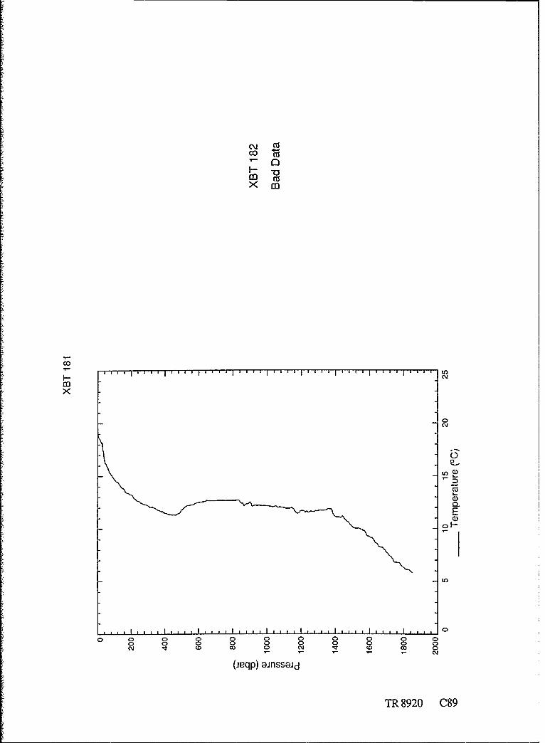
c\J (TS
Xco
Co
120
LA
EoF-
0 0 0 0 0 0 0 0 0 0m wD OD 0 Nq Nr to D 0
(ieqp) GaflSSE)Jd
TR 8920 C89

mc
C) 0 > CD, C> 0)
00
-0)
09 0R 892000 0 C

(D
a)
Ea)
o-
to
0 C0 0 0 0 0 0 0 0 0 00) 0 C0 0 0) 0 0 0 0> 0Nm 'T to 0 cm I (D co
(ieqp) aJflssaGc
LOco
N
too
, (
a)CL
0 0 0 00 0 0 0 0 00 0 0 0 0 0C 0 0 0 0N4 1 wD O 0 N to co 0
r r - - N
(ieqp) Galssaijd
TR 8920 C91

coCC)
0
E
U)
o 0 0 0 0 0 000 0 C 0 0 > 0 0 0 0cm 'I CD co 0 cm co 0o 0
mcxjq)anSJ
CC0
0
Ci)
0)(D
=3 caj(D
0 0 0 0 0 0 0 0 0 0 0C0 0 0 0 0 Q 0 0 0 0>04 to co 0 04MC CD 0
(jeqp) 9JflssOJd
C92 TR 8920

0
0
LA
Ea)
oC 0 0 C0 0 0 0 0 C0CcJ C> cm 0I CJ co CD
com
mcx
0
(1)
C-E
U)
0C)00 0 0 0 0 00 ) 0 > 0 0 D 0 0 0> C 0ND CD 0 C 'U Ci NT D co 0
r - cU
(jeqp) Gaflss@Jd
TR 8920 C93

c'J)
0)0
CY
0
0))
L2H (V
CL
E
LO
0 0 0 0 0 0 C 0C 0 0(NJ (0 to 0 (m IT co C >
(jeqp) ajflss@Jd
C94 TR 8920

CMJ
U)
CV))
cm
0
CVC)
0)~
mcXjq)ans~
TR 890 C0

100
x
L
a)
U)
0 0 0 0 0 0 C0 ) 00 0 0 0 0 0 0) 0
Nl IT w co 0 cm It to c C >
(ieqp) ejflss@Jd
LO0)
x
a)
a-a)CL
0 0 0 0 0 000 0 0 0 C 00> 0N~ (D co 0 N~ CD co 0
(jeqp) ejflss@Jd
C96 TR 8920J

aY)
Dox
0(\i
a)
Ea)
oH
I I I p I I I p p p S I a
0 0 0 0 0 a 0 0 0 0 0o 0 0 0 0 0 0 0 0C~l co c 0 cm t CD 0
(ieqp) ejflss@Jd
aa)
0 00 03
CUj
(jeqp) inss@)
TR 8920 C9

00
F--
mc
x
to~
0)
0 0) 0 0 C 0 0 0 0 00m 0 o 0 O0 0 0 0t 0o 0o 0
(jeqp) ajflssOd
C90 T 82

x
0l
t2J
03
o
CL
0 0 0 0 0 0 0 0 0)Nl CT D co 0 N~ (D OD 0
(jEqp) a.inssaldj
0
x
0 0
0 C) C>cmc 0 C1to O
C)(jeqp ainsaia
TR 890 C9

.. I 1
.* -T-rT -T-l,-T---sTI, IlL *f) *
x
Cj0
a)0.
0f)
CD
(jeqp) GaflssGJd
cr)0
x
a)0.E
0 0 0 0 0 0 0 0 0 00 0 0 0 0 0 0 0 0 0
w' (0 cD 0 cI wD OD 0
(ieqp) aJflssOJd
C100 TR 8920

(0
0C~J
a)
LO
0 0 00 00 0 0 0 0 0 C0 0 0D
0m 0 o 0 0 0 0 0 0o 0
(jeqp) Gaflssaic
TR 8920 ClOl

030
x
0
0f)
E
0 0)
o 0 0 0 0 0 0 a 0 0D0m 0T 0o 0 0M 0T 0o 0o 0
(jieqp) Oaflss9Jd
x
0q
E
to
o 0 0 0 0 0 0, 0 00 0 0 0 0 C0 0 0) 0
Nm IT D cD 0 ( D cD 0
(jeqp) aiflss@Jd
C102 TR 8920

mc
a-
Ea3)
0 0) 0 C 0 0 0 0 0 oCl D co 0) 'M 'IT co 0
(jeqp) Gaflss@Jd
O*) wl
N C)
x m
TR 8920 C103

Cuj
x
cis
D
En
0 0 0 0 CDP 40 0 0 0 0o C> 0 0 0 0 0 0 0D 0 0
0M 0 o 0 0 0 0V 0I c0 0o 0
(ieqp) aI1ss9Jd
F- cx
0cm
0
L
0)
Ln
0 0C 0 0 0 0 0 0 0 0 00 0) C 0 0 0 0 0 0 01m W0 co 0 N' * T (0 co 0
(jeqp) ejflss@Jd
C104 TR 8920

C)
X a
ce)
caJ
x
C-
oH
0 0 -) C C C)
(jeqp) aiflssOJd
TR 8920 C105

CD
x
CL
E
0 0 0 C0 0 0 C> 0 0 0 00 0D 0 0 0o 0 0 0 C> 0cm "T to5 co C0 0mo
(ie-qp) ajflssOid
Lf)
xo
C106 TR 8920

x
O.E
V ~ ~ C, C4 * 9 9 I a C> C>S I e VVVI a a Q5.
Q1 Q C> 0> C> C) CD C0
(jeqp) 8Jflssaid
I--m
x0
C-cm
=3olu
(D
0 0 0 0 0 0 0 0 0 0C) D 0 0 0 0 0 C> C 0)
(jeqp) Gaflssaid
TR 8920 C107

C>,
Cm"
x
CDO
a
E
0)0
co1
.1 x.. . 1** 9 .. * 19919*
0)0
CL
0 00 0 0 0 C) 0 0 . C) C
cm I (D o 0 m (D co0m
(jeqp) inssajS
C108 R 892

x
C>
Cl CD 0 0 C 40 C 0 C
Co C) 0 C) C. 0 Cl C CDCM "a co C CQ c co0
cm0
CML
I-- cm
0 0 0 C, 0 0 0 0 a0' 0 D 0 CJ CD 0 0 C. a
mcxjq)ansJ
T 820 C09

cmJ
x
E
)
0 C0 0 0) 0> 03 l 0 0 0 0cm 0 co 0o 0> 0m 0 o 0 0 0
(jeqp) GaflSS9Jd
C"
cmx
a)CLE
cm w co ~ I ~ I 0~ Icm (D IC 0
C110 TR 8920

(DCU,
x
CMJ
a)
Ea)
to
o 0 0 0 0> 0 0 0> 0o. o 0 0 0 0> 0 0 0> 0('j IT ( D 0 cm. IT to c 0
(jeqp) ejflss@Jd
Lo)
CM"
mcx
0cm
L0-
a
to
0 0 0 C0 0 0 0 0 0 0 0)0q 0 0o 0 0 0m 0 D 0 0 0
(jeqp) a ifssOJd
TR 8920 Clii

c'Jo
mc
EDE
0
CVj CD co 0 CVj (D U) 0
(JLqp) aJflSS@Jd
Cl 2 TR82

C\jC\jM
F- C'.
co%
0
0)
)
0
0 0 0 C) 0 C) 0 0 0 0 00 0 0 0 C> 0 0 0 0 0
CD t 03 0 CM 11 D 00 01 - - - - C
(j'eqp) aJflss9Jd
TR 8920 C113

APPENDIX D
Profiles of Sound Speed versus Pressure
Type 02 XSV depths were corrected and converted to pressure in the followingmanner.'First, -we solved for time of fall by inverting the fall rate equation to obtain
t -pcall + Npcall2 - 4(pcal2)(pcal0 + XSV depth)
2pcal2
where these pcal's are Sippican's XSV fall rate coefficients and have the values
pcal0 = 0.0pcall = 5.5895pcal2 = -0.00147.
Then we computed the new depth from time.
New XSV depth =-[(pcal0 + (pcall x t) + (pcal2 x :2)],
where these pcal's are the Cadiz cruise XSV coefficients determined in Section 5.1 andhave the values
pcal0 = 3.38pcall = 5.8561pcal2 = - 0.000883.
The "new XSV depths" were then converted to pressure in the same manner as the XBTdepths. The type 03 XSV depths were not corrected; only the conversion to pressure wasmade. The sound speeds for both the type 02s and 03s were adjusted by adding0.2 m s . The data were then gridded into 2 dbar values. The graphs have been ter-minated at the end of good data.

>cov
x
'7
In o
0 E
U)
C, C)
8 0
Cl
00
C,
(iqp U)ssi
00
0
U)
0
0)o
U)
0 00 C', 0 C: 0 Cll 0 CS
0
04 r 00 04 o-Col
(jeq) aissa0
TR 8920 D

>0Cl)
0)0
UJ) t2x
U)
G-
CD
0 0
t20)
0 0 0 0 0 0 0 0 0 0CQ 1 (D OD 0 N~ U) oa
(jL~qp) aJflss@Jd
D2 TR 8920

> C.)
Cl0)
CM
CL
000
0)0)
0 0 0 0 0 0 0 00
0 0 0 0 0 0 0 0 0C) 0 D 0 N 0 0 0 0
(jeqp) aJflss@Jd
I 1rI -Tr oI
0E
U)
vc)
0
0 0 0 00 0 0 0 0cm ITN CD 0 0 Nm co 0) 0
-~ r -m
(jeqp) aiflSSOJd
TR 8920 D3

(0 U)
0cm
lcj,
o :-00
LO )
0
co
CeU)
0 E
cvo0 0
C 0 0)cm (D co N o cU)
Comxjq)ensJ
D4 TR 890

(C0
U) !U2
x
o0
;c
00
0
0 0 0 0 0 0 0 0 0 00 0 0 0 0 C0 0 0 0 0
(ieqp) 8Jflss@Jd
LO)
x
00
U)0
0 - )cm w c 0 cmw co
cm(i~eqp)ajnss@)
TR 8920 D

col
U)
C,)>x)V
0)
CID
00
U) LO
-0
CL
U)
0
0 0 0 0 0C 0 0NCCI 0 C'j (D D 0
(ieqp) ejflssGJd
06 I.. 8920*

0
I * * *~ ~~ ~~ I Z1 . 11 1 1 I I~ III p ****
C,(j) 0)
It)
C-
C~
U)0
'-)
CL
0 0 C0 0 0 0 0) 0 0 0 00 0 0 0 0 0 0 0 0) 0
(eqp) ajflss@Jd
0)820 D

x
Ln
EU) 0
C)
CL
-00
0co
o o 00 0 0 0 0 0~j I o O 0 (~j - CD co 0
(aeqp) ajflss@Jd
C\j0
x
0
)
0
C5
U,
0 000
0m 0 o 0 0 0 0 0q 0 0
(jeqp) ejflssGJd
D8 TR 8920

c~cm
CDCo ULx -0
0
U) o
0)
03I t ICI
0 0 0 0
CMC
CfCix0
00
cm~ c 0 CI CO CD 0
c~cmC\Jp insac
TR 8920 D

CD.
x
0)
C)
C
0 :3C)02co)
0 0 0 0 0 0 0 0 0 00 0 0 0 0 0) 0 0 0(m IT 0 D 0 ('m IT to 0
(ieqp) aJflss@Jd
Lt)c\j0
L
x
0(m
/)
0
.Ul)
C:0 :300
C)
00 0 0 0 0 0 0 0 00 0D 0 0 0 0 o 0 O0 0
(jeqp) ejflssGJd
D 10 TR 8920

C 0M
0
0
U) o0 0 C) 0 0 0)0 0 0 0 0 0 0
C)
0
0
CM
(eqp) OajfSS8Jd
TR9- I

0cr)0 C
> V)
x
0E
aI)
'0U)
C
o 0 0 0 0 0 0D 0 0 0 0cm to CD 0 Nv w C3 0
(i-eqp) aflssGJd
(3))Ni
00
Clt)
SE
a0)
CL
000) U
0M 0 0 0o 0 0 0 0 O0 0
(jL~qp) aiflss9Jd
D12 TR 8920

CJ CZ
>0(/) 0x Z
x
U')
CL
0U)
0
0 0 0to w co 0 No co
(jeqp) OaflSSGJd
TR8920 D13

't'
UI)x
U)
7
CL
U)
0U) U
0 8 0 0 0 0 0 0 000 0 0 0 U0 0
(ieqp) eaflss@Jd
ce)CV)
> C9
NU)
a)0.
~0
0 0 00 0 0 0 0 0Nm wD c 0 N C> D
(jeqp) GaflSS9Jd
D14 TR 8920

ce))
LO
xQ
0M
(I)
C)
0 3 a 0 0 0 0 0 0 0 00 0 0 0) 0 0 0 0> 0l Cm CD co 0 NCD co 0
(jeqp) alflss9Jd
ccr)
to -Ux
F U)
n~~~C 00> 0
C>0 0 0 0 C, lc o 0 0uCD C
TR 8920 D15

Ce)
U))
U)
00
0 C))cm c co C ~ U> o C
CD
0 o C> 0C0 > 0 0 0 0> 0>C). C Cl 0 CD3 C C> 0
(jeqp) ajflss9Jd
16 R 92

0
x
CM
CJU)
C)C)ot-
0 0 0 0 0 0 000 0
0D 0 0 0 0 0 0 0 0 0Cq I CD co 0 cmJ (0 co 0
(jeqp) GaflssGJd
0
0CV')C0
x
C',
U)
U)
0.
C) C
* *~ * * * *~ * * * (j~ q p ) a J t s s @ J d 1
TR 920 D 17

Ul)U)
x0
Co
o
C
0)
co
0 0 l CD 0 0 0 0cq ~ ~ ~ ~ 01 t o 0 mw O
r co
cm)to
r0
C-
(I)
L 0 0. C 0 0 0 0 0
(aeqp),qsij
D18 TR 8920

00
U) c
[ 0)> Cl)
CL00
C)0U) U
0 0 0C 0 0 0 0 00) 0 0) 0 0 0 0 0 0 0,N~ (D0 c 0 cm IT co 0
lz (jeqp) aJflssaid
TR890 1

> C0
x
)
U)
co
CM
0 rT-0
N U) U 0 N D U)
to --
Lfa)
0
C)
-C
0 0 00 0 0 0 0) 0
D0 TR 8920 D U 0 N D U--- - N

00
xj
-1 LO)
C)
(DCL
U)
0
co
0 0 0 0 0 0 0 0 00 0 0> 0 0 0 0 0 0 0N~ (D co 0 cm qT D OD 0
(jeqp) ejflssOJd
x
H0 ECD
a/)
Co)
0U)
0 0 0 0 0 0 0 0 0 0 00 0 0 0> 0 0 0 0 0 0N ~ (JD CD 0 N~ (D CD 0
(jeqp) GJflSSOJd
TR 8920 D21

0LO)
UU
0
Uf)
CL
-U)
00
0
* .. .,, I I* ii I *9 I ag
0)
CD)
U) -U)
x8 0 0 00C~j D co 0 C ~ IT o N
U)j
(jeqp) inssai
D22 TR 892

c'JLO0
Uw)>..
x
0 E
(D
C,
0)
0 0.
C~
LfU)
0l)
to
C)
(0L
o04
U)
C
0 000
0
(jeqp) inss0)
TR 890 D0

U)f
0
CJ
'U)'a
0~
0
0 0 D 0 0 0 0 0 0o 0
(jLqp) ainssaid
co)
U)
x
0E
C-
t2U)
coC)D
0 0 0 0 0 0 0 0 0 00m 0 0 0 0 0m 0 0
(jeqp) ainssaid
D24 TR 8920

LOUr)
> CU)
x
to
2U)
0
0 00
0C0 0 0 0> 0 0 0 0cm 0 c 0 (Nm ' (D 0o
(Nm
(jeqp) aJflssijd
TR 8920 D25

APPENDIX E
Profiles of Temperature, Sound Speed, and Computed Salinityfor All Good Drop Pairs
The XSV probe depths were corrected individually, using the data from simultane-ously dropped XBT probes as described in Section 5.1. The data have been gridded into2 dbar bins. Salinity is averaged over 50 dbar; temperature and sound speed are averagedover 20 dbar. ,Salinity was determined as described in Section-5.4.

0
coM) l
x* W~a 0CL E-
CL )
_ a :
Ini .. H o
0' 0 000
10 0
LO C) 10m0
0006)
0 '
CD 0)0CD a
CO U) t
ca a
00
o6o
C)-0 0 -' a) 0'-
'-qp aaSSJ
TR 892 E I

o, )I F I I ..IL
Ue)-
CO 0 CE
U) E E0) CL
0
0 -)C
0 0) 0 0 0) 0 0 0> 0M (D CC) 0 Nq LO (o 0
(jeqp) aiflSS@Jd
(0~U 0)I ~0 UO
0
0 0 0
co /-.. \
co -n -- /
060
COO
CL
0
0~~~t 0 0 0 0 0
0 0 0 0 0 0 0 0 0
N (D 0 0o N (D c 0
(jeqp) aJflSSDJd
E2 TR 8920

C.o CU1 IC
o D 1
x c
06J
x 0.
CL
CD)
C) 00
0) 0 n CC. U) 0) 0 C
060
I-- CD 0 ' C C
ca cc CVC.x
0
x-C 0 0E
CL X
C-.L
Cl) .. . . .
C.) 0
U) a' 0)
0) 0 0C 0 0 0 0C0 00V 0D C 0 0\ CD CD 0
(jeqp) aJflssaid
TR 8920 E3

LO Cl M w
Cd)
050
m U . N U
- -3
j) EO
C: 0
U))
0~~~D 0co t2 U)0)U) U
00C0 N
m~ N0 U)m(0 c
U)O 0
'6o 0) (1)
'I 0)) (j
N' 0.
U) U
060
W ) U) 0
cn 0 -
ClU)
0a (1)N CO U 0 N ) U)
(eqp eUlS8J
E4 TR892

cc
x j06
a- EUa) 0'
I)I
CL - C)/E
(') 0) 0 0
C)2Q
0 0) 0C0 0 0 0 0 C0cm v (D co 0 cm co co 0
(jeqp);gjnssEGJd
060
0
H o CD Uco -ocm
06
C/0)x 0.
U) 0
CD 00
N IL
U) E)
00
M Ln CD
0 0 0 0 0 0 0 0 0 0N co cD 0 N(D co 0
(jeqp) Geflss@Jd
TR 8920 E5

C) I 111111T= LO 00)1
06
I-0CO cAC"
x06 /-
x U) *\/E
C0. D1
C £1)
UU)
co C) 00
to (0 ct0nN o 0
0C-)D
oq (D c mIo c
CD
05~
ca cm Mx06 --
U)2
x 0.-' 0 . E
CL
0 =
0- C) 01
00
0 0)
0 0C 0 0 0 0 0(NJ to 0o 0 (NJ to co 0
(ieqp) ajflss@Jd
E6 TR 8920

CV) cl CV
060
00
x
/ 0 ECl)
cu--w)
U) E
C)C - i 3,
[ C)
o 0 0 0) 0 0 C0 0 0C) n Co 0) 0N CD C 0
(jeqp) ajflss@Jd
0) . . . . .t
06CMJ
0~c ./ 0
x
x -. 3 0
0) - ECLI
E vE00=
C)0
In ton
0co
0CD0 0 0 0 0 0 CD0 0 0 0 0 0D 0 03 0 0)
Nm W0 i 0 N ~ ~ D c 0
(jeqp) aiflSS@Jd
TR 8920 E 7

C6 ULO)
0
C5/-X
0
Ea)
cu~
U) C
C9 0 0 Zo0)
0 0 10\ CD ) 0 C 0
(jeqp) GaflSSGJd
ot
050
0
/o Eco I) (3 M0
0.- ))- -
E
U)
If))
C>
0
tn 0
0 0 0 0 0 0 0 00 0 0 0 0 0 0 0 0 C0C'J * t (D 0) 0 N ~ (D 0
(ieqp) aJflSS@Jd
E8 TR 8920

o ~~~~~~~~~~~~~~~~ .~ .**t . LO aj. ag.-S * . da j t. ~~ aB I) *2
*C o W c'
C'jo C6-.s
1- i
Z1- ---
U) S .f)
cn Es
CL
0 ~ ~~~~ 00 0 D > C
0 m to 0CD 0 cm 0 o C,
(jeqp) ajnssJd-
(I) U).
. 1 . . It
0Ci)- CD 0 c
A co- ~
x E)
f C13 (1
U) Ea) C
coO
C')
0 0
0 0 0 0 0 00 0 0 00~ 0 o 0 0 0 0 0~ 0C 0
(jeqp) a~inssaJd
TR 8920 E9

cii0
(a)
06
0
4) 0
U)'
C.,L
-) 0
U)
0 0
-c
C3 C)0. C/m (D c '3 vc c
A) LO
06)
0 0 0
S (D 03 )
(0 0
(i~qp) (Dsai
0o 0 0 00
ElO TR8a)

C)
x C" U
X =3
U) A Wj
C C/
EC3 0) 0
';2 U)
C')qp OclSG
CC) CD Coh* * l ; hI,.,aUom CD c m)D cc~cm
co a) .I ICI) c
o0 ~
ca C 1 ' I) CMx /~
U)
o
U)C/
,00
0 0 0 0 0 0 0 0 0 0C,0 0 0 C 0 0('U CD CD 0 CDj (0 0
(jeqp) Gaflssaid
TR 8920 Eli

f .) .1 U 0
C0ICv)
o o CM -
00N
m N U
C,) (1) E
0 . C 13 0 D
C ...... C0..a. .......... . a)*
I 1 C0
So~
Cj O 0o 00)
U) 0)
C'M
060co2
00 C~0
060
U))x ) I N 0 E
C~U)C~CL
o -E-.
H / 0 0
C~ )
Cl0)
0) -) C2(
C) 0 C
0 0 0 0 0 0 co 0
(jeqp) aJflSS@Jd
E12 TR 8920

CV)
coo~
x U- U
(1- =3 0
a)
cu C
0
CD 00
o0U))
C, !
0 0 0 0 0. 0 0 0 0 0 00) 0 0 0 0D 0 0 0 0 0cm (D co 0 01 v t 0
(ieqp) Oaflssaid
0 U)
CYU)
m o cm Ux
U) 0
0.: , LO 0-
LACL
U)~~~ .... ......
C)a 0
0)
CD 0~
00
C) 0
0 m 0(0 0 0o 0 0 0 D 0 0
TR 8920 E13

CM a) . - - I . . I . . I I . I . ) I . N . I . I . .IL
Cl) C
06
>
U)U
X C/0
0
-L 0
0D 0. .. 1 00 0 0o 0 0
0) W 0)
- C.M
m co
CY
0 00
060
ClCD
CIJ~~~c CDC i D C
(Uqp CJlSLJ
E14 TR892

ID rwr-Tr--T---F 0 IIII tc))
co
x -l L
U)j
0I ) 0~-
Ci)
U) CL -)E
0)
0 0 0 CD 0 0 0 0 0 0 00 0 0 c 0 0 0 0 0 0cm (0 0 cm (D c)
c'J m
00- -
02 Noc U)x .1
U/ C) Ux =3 0
a) a)
0
00
M U)
0 0C0D 0 0 0 0 0 0 00 0 0 0 0 0 0 0 0
N 0 ) 0 oC (D 0o 0
(jeqp) aJflssaid
TR 8920 E15

06
C
x = 0 0
Cl- /l CU)
LtLL
'.- C.
C) Eo
0)
Mn Ln 0C')
0 0 0 0 0 0 0 0 0 000 0 C 0 0 0 0) 0 0Nv (D co 0 m to CD 0
(ieqp) Oaflss@Jd
06)
coJ
0 0t- ~ A\0 Nm
06 />A
C)
CC
oO
0 00
C9)
C')
0 0 0 0 0 0 00 0 0 0 00 0 0 0 0
N4 to OD 0 NM to 00 0- r N
(jeqp) aJflSSaJd
E16 TR 8920

060
00F- . /o
ro N_~ U)
0.
C/)D
* ()E
Ao 0: 0
U)0co) to 0)
C>0 0 0 0 0 0 0) 0 0 0 00 0 0 0C 0 0 0
Nq (D co 0 qC CD
(jeqp) ainSGJd
0)
0) 0) C~)
U ) 7u)
x :3 0
x) E
Cl)-- 7 0 cO
Q/ U))
(I) E
0 o0
co Uc
C 0)CD CC)a
0 0 0 0 0 0 0 0 0 0N CD CO) 0 N ~ (D CO 0
(jeqp) Gaflss@Jd
TR 8920 E17

C'i a, ... I .... ~ I .I .. .IIIIII.It 0
0
x NN
U)I
U) - - ECL (D C
cu a)
) 0)
co
0 0 0 0 0 0 0 0 0 0 00) 0C0 0 0 0 0 0 0
l (0 co 0 cm (D 00 0
(jeqp) aJflssaid
0
H 0mo cj cm t
U) U
CO
.*.* * ~.. a)
0C-3 If
00 0 0 0 0 0 0 0 0 00 0 0 0 0 0 0
N~ (0 (0 0 (D c) 0r -- -N
(ieqp);gjflss@Jd
E18 TR 8920

LO0
060
C.) C/U
/ E
C N)
U) .. . . .E.. . C
0- 0(v)L' U)/
to 0C.)
0 0 0 0 0) 0 0 0 0 0 00 0 0 0 0) 0 0 0 0 0CUj (0 00 0 cm (D c0 0)
(jeqp) ainSSOJd
co) 0)N c
C.) co U)
0)
0
02 cmx
U)-0. E
C.C>
C~L CL -
a))U
- C
o0
co U) 0
00
0) 0C 00 0 0 0)
cUi CDj 0) (0 co 0
(ieqp) eJflssOJd
TR 8920 E19

04 ~04 0
m CD)ccn LO .* '>i.04 IU)*.
x 0Il* ' a.**-
ca CLU)
cub I oc 8
CD 0
V -o
0 0
0 0 o 0 o 0 0 0 0 o 0
(jeqp) ainss@Jd
In
o o 0CDm 0 0
x 07E
/ CD
U) .. . ..CD 0 HCD
In 0
0) In a)
CO 0
0 0 0 0 0 0D 0 0 0 0 00 0 0) 0 0 CD 0 0 0 004 (a D CD 0 04j at D CD 0
- - - a- 0
(jeqp) 8JflssEJd
E20 TR 8920

060
LO5
CDo 0 C)060
/ ECLl~
Cl0)
C/) N a. U)0))
U) 0I 0
c))
U) 0
L00to
0 0 0 0 C) 0 0 0 0 0 0o 0 C0 0 0) 0 0 0 0cm U) oa 0 (V ) )
(ieqp) ejflssGJd
C) *.j (VC\J
Ur)
x/
/ 0U) E
VaC L.L
U)
_ E
cl0
00
0 0 0CID coU) a 0 (V a CID a) 0
(ieqp) aiflssOJd
TR 8920 E21

V
C\j cm IN(\j -tU)
LC)
H 0
x-06
U)-' * 'I6
7 -' E
CC
a) c
0
0
_ _ _ _ _ _ I__ _ _ _ _ _ _ _ _ _ _ _
00 0 0 0 0 0 0 0 0 o0 0 0 0 0 C0 0 0 0 0cm to cC 0 N (D c)
(jeqp) aiflSGJd
E22 TR 8920

APPENDIX F
Algorithm-for Computing Salinity from Temperature,Sound Speed, and Pressure
I

Chen and Millero (1977) give an empirical relation for computing the sound speed in sea-
water from the measured values of the seawater temperature, salinity, and pressure. To estimate
the salinity of the seawater from measured values of sound velocity, temperature, and pressure,
their relation is inverted, so that salinity is found as a function of the other three variables. Chen
and Millero (Eq. 4) give
(U p - U~H20 ) -H(U - U°2o) = AS + BS 1 "5 + CS2
where
u p = speed of sound in seawa:sr
H= speed of sound in pure water
U° = speed of sound in seawater at zero pressure
Uo = speed of sound in pure water at zero pressure
S = salinity
A, B, C = coefficients.
The term U°0 - U° 20 is also given as a function of S, S1 5, and S2 Solving for S, the equation can
be rearranged asCS 2 + BS' 5 + AS - (Up - Up)+(U - 2 )=
or
S2 + a S1 5 + bS + d = 0.
The coefficients a, b, and d are computed from parameters given by Chen and Millero.
The following is a function written in C which, when given values of sound speed, tempera-
ture, and pressure, will return a value of salinity obtained by numerically solving the above
equation. The program that calls the function is not given.
TR 8920 F1

** sfsvel.c'
** Source C.-T. Chen and F.J. Millero (1977)** Journal of the Acoustic Society of America** Vol 62, pp 1129-1135.** ( inversion of their equations
** Check values sfsvel( 1521.46, 20., 0 ) = 35.0** sfsvel( 1506.34, 10., 1000 ) = 35.0** sfsvel( 1503.87, 5., 2000 ) = 35.0
/* -- Equation (4) in Chen and Millero is
u - upure )-( uO - uOpure ) = A*S +B*SA1.5 +C*S^2
where u =speed of sound in seawater water,upure =speed of sound in pure water,uO =s'eed of sound in seawater at zero pressure,uOpure =speed of sound in pure water at zero pressure,S -salinity, andA,B.C =coefficients
Solving for S, the equation can rearranged as
C*S^2 +B*S'^1.5 +A*S (u -upure) + (uO-uOpure) 0.
or S^2 + a*S'^l.5 + b*S + d =0
# include "'math.h t
# define EPSi 1.0e-06# define EPS2 1.0e-10
double sfsvel( u, t, p
double u; /* sound velocity in rn/s *double t; /* temperature in deg. C *double p; /* pressure in dbars ~
double sqrto;double u_pure;double a, b, d, factor, 5, si, s2, s3, s3_old, fO, fl, f2, f3;int flag = 1;
/* -------initialize parameter coefficients----------*
double ul = 1402.388, u2 = 5.03711, u3 = -5.80852e-2;double u4 = 3.3420e-4, u5 = -1.47800e-6, u6 =3.1464e-9;double u7 = 0.153563, uS = 6.8982e-4, u9 = -8.1788e-6;double ulO =l.3621e-7, ull = -6.1185e-10, u12 = 3.1260e-5;double u13 = -1.7107e-6, u14 = 2.5974e-8, u15 = -2.5335e-10;double u16 = 1.0405e-12, u17 = -9.7729e-9, ulB = 3.8504e-10;double u19 = -2.3643e-12;
double dl = 1.389, d2 = -1.262e-2, d3 = 7.164e-5;double d4 = 2.006e-6, d5 = -3.2le-8, d6 = -1.922e-2;double d7 = -4.42e-5, d8 = 1.727e-3;
double al = 9.4742e-5, a2 = -1.2580e-5, a3 = -6.4885e-8;double a4 = 1.0507e-8, a5 = -2.0122e-10, a6 = -3.9064e-7;double a7 = 9.104le-9, a8 = -1.6002e-10, a9 = 7.988e-12;
F2 TR 8920

double alO =l.100e-l0, all = 6.649e-12, a12 = -3.389e-13;
double bl = 7.3637e-5, b2 = 1.7945e-7, ci = -7.9836e-6;
/*-------------------------------------------------------------*
p 1 10.; /*-- convert dbars to bars -
/* -- compute the speed of sound in pure water (Chen & Millero, Eq (3)--*
upure = ul + t*( u2 + t*( u3 + t*( u4 + t*( u5 + t*uE))))* ( u7 + t*( u8 + t*( u9 + t*( u10 + t*ull))fl*p+ ( u12 + t*( u13 + t*( u14 + t*( u15 + t*u16))))*p*p+ ( u17 + t*( u18 + t*u19))*p*p*p;
factor =cl*p + d8;
a d6 + t*d7) + (bl +t*b2 *p;a 1=factor;
b = dl +t*( d2 + t*(d3 +t*(d4 +t*d5))+ (al +t*( a2 +t*(a3 +t*( a4 +t*a5))))*p+ (a6 + t*( a7 + t*( a8 + t*a9)))*p*p+ (alO + t*( all + t*a12 ))*p*p*p;
b 1=factor;
d =uypure - u;d 1=factor;
1* Need to solve equation S^2 + a* S~l.5 + b*S + d =0with the desired root between S = 0 and S = 40.
Solution is obtained by modified linear interpolation methodas shown in "Applied Numerical Analysis (Second Edition)"
by C.F. Gerald, Addison-Wesley Publishing Company, 1978, 518p. *sl= 0.;
s2 = 40.;fl = sl*sl + a*sl*sqrt( si + b'~sl + d;f2 = s2*s2 + a*s2*sqrt( s2 )+ b*s2 + d;fo = fl;
s3 = si;s3_old =s2;
if( fl != 0. H(while(C flag 1=I
s3 = s2 -f2*( s2 -1 )/(M f2 - flif( s3 < 0. ) return( atof( "-l.e30", ) ; * -- return bad value *f3 = 3*s3 + a*s3*sqrt( s3 )+ b*s3 + d;if( f3/fl < 0. )
s2 = s3;f2 =f3;if( f3/fO > 0. )fl *= 0.5;
else(si = s3;fli f3;if( f3/fO > 0. 1f2 *= 0.5;
fO =f3;
if( fabs( s3 - s3 old )< EPSI 11 fabs( fO )< EPS2 H(S5 s3;break;
return( S )
TR 8920 F3

UnclassifiedSECURITY CLASSIFICATION OF THIS PAGE
Form ApprovedREPORT DOCUMENTATION PAGE OMBNo 0704.0188
la REPORT SECURITY CLASSIFICATION lb RESTRICTIVE MARKINGS
Unclassified2a SECURITY CLASSIFICATION AUTHORITY 3 DISTRIBUTION/ AVAILABILITY OF REPORT
2b DECLASSIFICATION/DOWNGRADING SCHEDULE Distribution unlimited
4 PERFORMING ORGANIZATION REPORT NUMBER(S) S MONITORING ORGANIZATION REPORT NLMBER(S)
APL-U11 TR8920
6a NAME OF PERFORMING ORGANIZATION 6b OFFICE SYMBOL 7a NAME OF MONITORING ORGANIZATIONApplied Physics Laboratory (If applicable) Office of Naval Research
University of Washington (Code 1122PO)
6c. ADDRESS (City, State, and ZIP Code) 7b ADDRESS (City, State, and ZIP Code)
1013 N.E. 40th Street 800 North Quincy StreetSeattle, WA 98105-6698 Arlington, Virginia 22217-5000
8a NAME OF FUNDING JSPONSORING 8b OFFICE SYMBOL 9 PROCUREMENT INSTRUMENT IDENTIFICATION NUMBERORGANIZATION (If applicable)Office of Naval Research N00014-87-K-0004
8c. ADDRESS (City, State, and ZIP Code) 10 SOURCE OF FUNDING NUMBERS
PROGRAM PROJECT TASK WORK UNIT800 North Quincy Street ELEMENT NO NO NO ACCESSION NOArlington, Virginia 22217-5000 422PO .... 06
11 TITLE (Include Security Classification)
XBT and XSV Data from the Gulf of Cadiz Expedition: R/V Oceanus Cruise 20212 PERSONAL AUTHOR(S)
Maureen A. Kennelly, Mark D. Prater, Thomas B. Sanford13a TYPE OF REPORT 13b TIME COVERED 14 DATE OF REPORT (Year, Month, Day) 15 PAGE COUNT
Data FROM q/aSTOQ August 1989 20916 SUPPLEMENTARY NOTATION
17 COSATI CODES 18 SUBJECT TERMS (Continue on reverse if necessary and identify by block number)
FIELD GROUP SUB-GROUP Meddy 7 Salinity profiles -)Cape St. Vincent,
08 03 XBT profiles 9 Gulf of Cadiz " Portugal ,XSV profiles Ampere Seamount
19 ABSTRACT (Continue on reverse if necessary and identql by block number)
Temperature profiles from expendable bathythermographs (XBTs)and sound speed profiles from expendable sound velocimeters(XSVs) were obtained during leg 1 of the Gulf of Cadiz Expedi-tion, 4-19 September 1988, from R/V Oceanus. XBTs and XSVs weredeployed around Ampere Seamount and Cape St. Vincent, Portugal.Salinity profiles have been calculated from simultaneouslydropped pairs of XBTs and XSVs. This report describes theinstrumentation used, discusses data acquisition and processingmethods, and presents temperature, sound speed, and salinity pro-files. ,
20 DISTRIBUTION/AVAILABILITY OF ABSTRACT 21 ABSTRACT SECURITY CL-ISSIFICATION0 UNCLASSIFIEDIUNLIMITED 5 SAME AS RPT El DTIC USFRS Unclassified
22a NAME OF RESPONSIBLE INDIVIDUAL 22b TELEPHONE (Include Area Code) 22c OFFICE SYMBOLDavid Evans and Alan Brandt (202) 696-44111
DD Form 1473, JUN 86 Previous editions are obsolete SECURITY CLASSIFICATION OF THIS PAGE
SIN 0102-LF-014-6603 Unclassified
Related Documents