• • The Measurement Perspective on Decision … Measurement Perspective on Decision Usefulness 177 FIGURE 6.1 PROSPECT THEORY UTILITY FUNCTION U(x) x loss gain power) is likely

The MeasurementPerspective on Decision

Usefulness

6.1 OverviewThe measurement perspective on decision usefulness implies greater usage offair values in the financial statements proper. Following from our discussion inSection 2.5.1, greater use of fair values suggests a balance sheet approach to finan-cial reporting, as opposed to the income statement approach which underlies theresearch described in Chapter 5. This, in turn, implies a larger role for the finan-cial statements proper to assist investors in predicting the firm’s fundamentalvalue, that is, the value the firm’s shares would have if all relevant information wasin the public domain. We define the measurement perspective as follows:

The measurement perspective on decision usefulness is an approach to finan-cial reporting under which accountants undertake a responsibility to incorpo-rate fair values into the financial statements proper, providing that this can bedone with reasonable reliability, thereby recognizing an increased obligationto assist investors to predict fundamental firm value.

Of course, if a measurement perspective is to be useful, it must not be at thecost of a substantial reduction in reliability. While it is unlikely that a measurementperspective will replace the historical cost basis of accounting, it does seem to be thecase that the relative balance of cost-based versus fair value-based information inthe financial statements is moving in the fair value direction. This may seemstrange, given the problems that techniques such as RRA accounting have experi-enced. However, a number of reasons can be suggested for the change in emphasis.

One such reason involves securities market efficiency. Despite the impressiveresults outlined in Chapter 5 in favour of the decision usefulness of reported netincome, recent years have seen increasing theory and evidence suggesting that

•c

h

apter

s

ix

••

ch

ap t e r

s

ix

•

• •

securities markets may not be as efficient as originally believed. This suggestionhas major implications for accounting. To the extent that securities markets arenot fully efficient, the reliance on efficient markets to justify historical cost-basedfinancial statements supplemented by much supplementary disclosure, whichunderlies the information perspective’s approach to decision usefulness, is threat-ened. For example, if investors collectively are not as adept at processing informa-tion as efficiency theory assumes, perhaps usefulness would be enhanced bygreater use of fair values in the financial statements proper. Furthermore, whilebeta is the only relevant risk measure according to the CAPM, perhaps accoun-tants should take more responsibility for reporting on firm risk if markets are notfully efficient.

Other reasons derive from a low proportion of share price variabilityexplained by historical cost-based net income, from the Ohlson clean surplus the-ory that provides support for increased measurement, and from the legal liabilityto which accountants are exposed when firms become financialy distressed.

In this chapter we will outline and discuss these various reasons.

6.2 Are Securities Markets Efficient?

6.2.1 INTRODUCTIONIn recent years, increasing questions have been raised about the extent of securi-ties market efficiency. These questions are of considerable importance to accoun-tants since, if they are valid, the practice of relying on supplementary informationin notes and elsewhere to augment the basic historical cost-based financial state-ments may not be completely effective in conveying useful information toinvestors. Furthermore, to the extent that securities markets are not fully efficient,improved financial reporting may be helpful in reducing inefficiencies, therebyimproving the proper operation of securities markets. That is, better reporting offirm value will enable investors to better estimate fundamental value, therebymore easily identifying mispriced securities. In this section, we will outline anddiscuss the major questions that have been raised about market efficiency.

The basic premise of these questions is that average investor behaviour maynot correspond with the rational decision theory and investment models outlinedin Chapter 3. Investors may be biased in their reaction to information, relative tohow they should react according to Bayes’ theorem. For example, psychologicalevidence suggests that individuals tend to be overconfident—they overestimatethe precision of information they collect themselves (see, for example, the discus-sion in Odean (1998)). If an individual’s information collecting activities revealGN, for example, he or she will revise their subjective probability of high futureearnings by more than they should according to Bayes’ theorem. If, on average,investors behave this way, share price will overreact.

The Measurement Perspective on Decision Usefulness 175

Another attribute of many individuals is self-attribution bias, whereby indi-viduals feel that good decision outcomes are due to their abilities, whereas bad out-comes are due to unfortunate realizations of states of nature, hence not their fault.Suppose that following an overconfident investor’s decision to purchase a firm’sshares, its share price rises (for whatever reason). Then, the investor’s faith in his orher investment ability rises. If share price falls, faith in ability does not fall. If theaverage investor behaves this way, share price momentum will develop.That is, rein-forced confidence following a rise in share price leads to the purchase of more shares,and share price rises further. Confidence is again reinforced, and the process feedsupon itself, that is, it gains momentum. Daniel, Hirshleifer and Subrahmanyam(1998) present a model whereby momentum develops when investors are overconfi-dent and self-attribution biased. Daniel and Titman (1999), in an empirical study,report that over the period 1968–1997 a strategy of buying portfolios of high-momentum shares and short-selling low-momentum ones earned high and persis-tent abnormal returns (i.e., higher than the return from holding the marketportfolio), consistent with the overconfidence and momentum arguments.1

Self-attribution bias and momentum are, of course, inconsistent with securi-ties market efficiency and underlying decision theory. According to the CAPM,higher returns can only be earned if higher beta risk is borne. Yet Daniel andTitman report that the average beta risk of their momentum portfolios was lessthan that of the market portfolio. Furthermore, share price momentum impliespositive serial correlation of returns, contrary to the random walk behaviour ofreturns under market efficiency.

The study of behavioural-based securities market efficiencies is called behav-ioural finance. For a comprehensive review of the theory and evidence of behav-ioural finance, see Hirshleifer (2001). We now review several other questionsabout efficiency that have been raised in this theory.

6.2.2 PROSPECT THEORYThe prospect theory of Kahneman and Tversky (1979) provides a behavioural-based alternative to the rational decision theory described in Section 3.3.According to prospect theory, an investor considering a risky investment (a“prospect”) will separately evaluate prospective gains and losses. This contrastswith decision theory where investors evaluate decisions in terms of their effects ontheir total wealth (see Chapter 3, Note 4). Separate evaluation of gains and lossesabout a reference point is an implication of the psychological concept of narrowframing, whereby individuals analyze problems in too isolated a manner, as a wayof economizing on the mental effort of decision making. This mental effort mayderive from information overload (i.e., more information than the individual canhandle) and/or from a feeling that it is not worth the effort to acquire more infor-mation. As a result, an individual’s utility in prospect theory is defined over devi-ations from zero for the prospect in question, rather than over total wealth.

176 Chapter 6

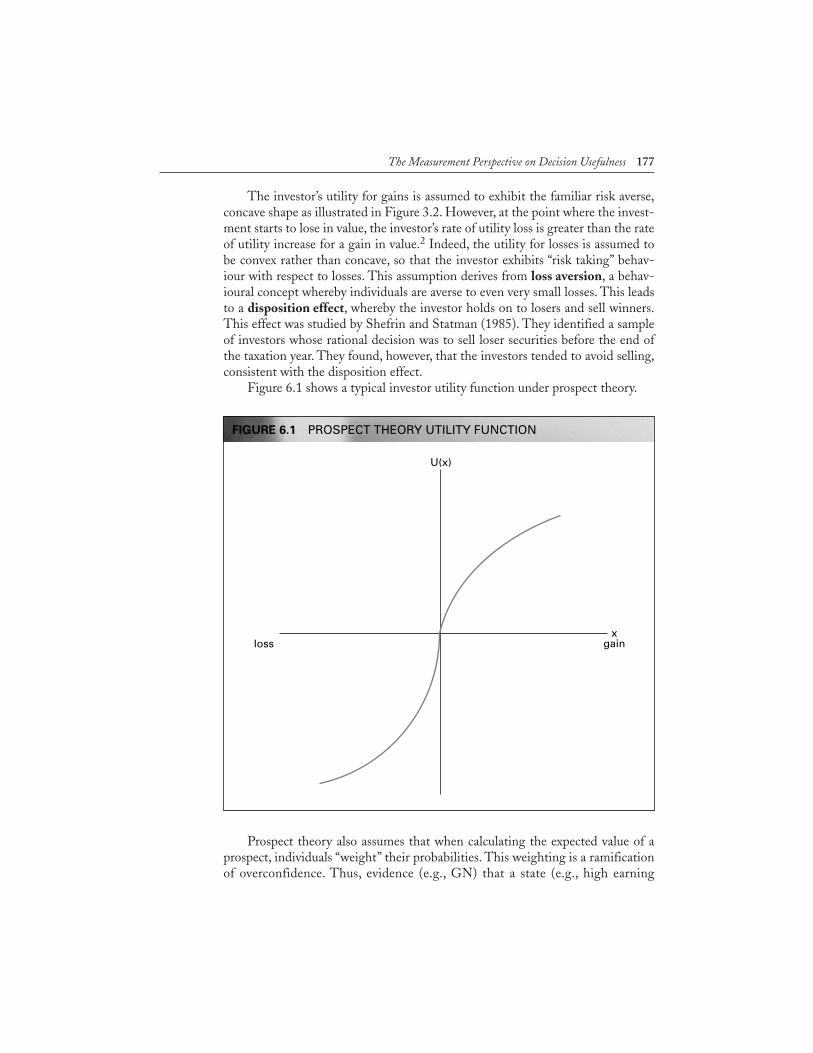
The investor’s utility for gains is assumed to exhibit the familiar risk averse,concave shape as illustrated in Figure 3.2. However, at the point where the invest-ment starts to lose in value, the investor’s rate of utility loss is greater than the rateof utility increase for a gain in value.2 Indeed, the utility for losses is assumed tobe convex rather than concave, so that the investor exhibits “risk taking” behav-iour with respect to losses. This assumption derives from loss aversion, a behav-ioural concept whereby individuals are averse to even very small losses. This leadsto a disposition effect, whereby the investor holds on to losers and sell winners.This effect was studied by Shefrin and Statman (1985). They identified a sampleof investors whose rational decision was to sell loser securities before the end ofthe taxation year. They found, however, that the investors tended to avoid selling,consistent with the disposition effect.

Figure 6.1 shows a typical investor utility function under prospect theory.

Prospect theory also assumes that when calculating the expected value of aprospect, individuals “weight” their probabilities. This weighting is a ramificationof overconfidence. Thus, evidence (e.g., GN) that a state (e.g., high earning


FIGURE 6.1 PROSPECT THEORY UTILITY FUNCTION

U(x)

x gain loss

power) is likely to happen will be underweighted, particularly if the evidence isabstract, statistical, and highly relevant. In effect, by underweighting evidencethat a state is likely to happen, the main diagonal probabilities of the informationsystem are perceived by the overconfident investor as lower than they actually are.As a result, the individual’s posterior probability of the state is also too low.However, individuals tend to overweight salient, anecdotal, and extreme evidence(e.g., a media article claiming that a stock is about to take off ), even though real-ization of such states is a rare event.

These tendencies lead to “too-low” posterior probabilities on states that arelikely to happen, and “too high” on states that are unlikely to happen. The poste-rior probabilities need not sum to one.

The combination of separate evaluation of gains and losses and the weight-ing of probabilities can lead to a wide variety of “irrational” behaviours. For exam-ple, fear of losses may cause investors to stay out of the market even if prospectshave positive expected value according to a decision theory calculation. Also, theymay underreact to bad news by holding on to “losers” so as to avoid realizing aloss, or may even buy more of a loser stock, thereby taking on added risk. Thus,under prospect theory, investor behaviour depends in a complex way on the levelsof payoff probabilities, risk aversion with respect to gains and risk taking withrespect to losses.

There are few empirical accounting tests of prospect theory, relative to theempirical tests based on rational investor behaviour described in Chapter 5. Onesuch test, however, was conducted by Burgstahler and Dichev (1997). In a largesample of U.S. firms from 1974–1976, these researchers documented that rela-tively few firms in their sample reported small losses. A relatively large number offirms reported small positive earnings. Burgstahler and Dichev interpreted thisresult as evidence that firms that would otherwise report a small loss manipulatecash flows and accruals to manage their reported earnings upwards, so as toinstead show small positive earnings (techniques of earnings management are dis-cussed in Chapter 11).

As Burgstahler and Dichev point out, this result is consistent with prospecttheory. To see why, recall first that prospect theory assumes that investors evaluategains and losses relative to a reference point of zero—if earnings are positive,share value, hence investor wealth and utility, increases, and vice versa if earningsare negative. Now observe from Figure 6.1 that the rate at which investor utilityincreases is greatest for small gains, and the rate at which it decreases is evengreater for small losses. This implies a very strong rate of negative investor reac-tion to a small reported loss, and a strong rate of positive reaction to smallreported positive earnings. Managers of firms that would otherwise report a smallloss thus have an incentive to avoid this negative investor reaction, and enjoy apositive reaction, by managing reported earnings upwards. (Of course, managersof firms with large losses have similar incentives, but as the loss increases itbecomes more difficult to manage earnings sufficiently to avoid the loss. Also, the

178 Chapter 6

incentive to manage earnings upwards declines for larger losses since the rate ofnegative investor reaction is not as great, and runs into a disposition effect.)

However, Burgstahler and Dichev suggest that their evidence is also consis-tent with rational behaviour. Lenders will demand better terms from firms thatreport losses, for example. Also, suppliers may cut the firm off, or demand imme-diate payment for goods shipped. To avoid these consequences, managers have anincentive to avoid reporting losses if possible. As a result, the extent to whichBurgstahler and Dichev’s findings support prospect theory is unclear.

6.2.3 IS BETA DEAD?As mentioned in Section 4.5, an implication of the CAPM is that a stock’s beta isthe sole firm-specific determinant of the expected return on that stock. If theCAPM reasonably captures rational investor behaviour, share returns should beincreasing in βj and should be unaffected by other measures of firm-specific risk,which are diversified away. However, in a large sample of firms traded on majorU.S. stock exchanges over the period 1963–1990, Fama and French (1992) foundthat beta had little ability to explain stock returns. Instead, they found significantexplanatory power for the book-to-market ratio (ratio of book value of commonequity to market value) and for firm size. Their results suggest that rather thanlooking to beta as a risk measure, the market acts as if firm risk increases withbook-to-market and decreases with firm size. These results led some to suggestthat beta is “dead.”

Different results are reported by Kothari, Shanken, and Sloan (1995), how-ever. They found that over a longer period of time (1941–1990) beta was a signif-icant predictor of return. Book-to-market also predicted return, but its effect wasrelatively weak. They attributed the difference between their results and those ofFama and French to differences in methodology and time period studied.

The status of the CAPM thus seems unclear. A possible way to “rescue” betais to recognize that it may change over time. Our discussion in Section 4.5assumed that beta was stationary. However, events such as changes in interestrates and firms’ capital structures, improvements in firms’ abilities to manage risk,and development of global markets may affect the relationship between the returnon individual firms’ shares and the marketwide return, thereby affecting the valueof firms’ betas. If so, evidence of volatility that appears to conflict with the CAPMcould perhaps be explained by shifts in beta.

If betas are non-stationary, rational investors will want to know when and byhow much they have changed. This is a difficult question to answer in a timelymanner, and different investors will have different opinions.This introduces differ-ences in their investment decisions, even though they all have access to the sameinformation and proceed rationally with respect to their opinion as to what beta is.In effect, an additional source of uncertainty, beyond the uncertainty resultingfrom random states of nature, is introduced into the market. This uncertainty


arises from the mistakes investors make in evaluating new values of non-stationaryshare price parameters. As a result, additional volatility is introduced into shareprice behaviour but beta remains as the only variable that explains this behaviour.That is, the CAPM implication that beta is the sole firm specific risk variable isreinstated, with the proviso that beta is non-stationary. Models that assume ratio-nal investor behaviour in the face of non-stationarity3 are presented by Kurz(1997). Evidence that non-stationarity of beta explains much of the apparentanomalous behaviour of share prices is provided by Ball and Kothari (1989).

Behavioural finance, however, provides a different perspective on the validityof the CAPM. Daniel, Hirshleifer, and Subrahmanyam (2001) present a modelthat assumes two types of investors—rational and overconfident. Because ofrational investors, a stock’s beta is positively related to its returns, as in theCAPM. However, overconfident investors overreact as they gather information.In the case of GN, this drives share price too high, thereby driving down thefirm’s book-to-market ratio. Over time, share price reverts towards its efficientlevel as the overconfidence is revealed. As a result, both beta and book-to-marketratio are positively related to future share returns, consistent with the results ofKothari, Shanken, and Sloan, and inconsistent with the CAPM’s prediction thatbeta is the only firm-specific return predictor.

From an accounting standpoint, to the extent that beta is not the only rele-vant firm-specific risk measure, this can only increase the role of financial state-ments in reporting useful risk information (the book-to-market ratio is anaccounting-based variable, for example). Nevertheless, in the face of the mixedevidence reported above, we conclude that beta is not dead. However, it maychange over time and may have to “move over” to share its status as a risk measurewith accounting-based variables.

6.2.4 EXCESS STOCK MARKET VOLATILITYFurther questions about securities market efficiency derive from evidence ofexcess stock price volatility at the market level. Recall from the CAPM (equation4.2) that, holding beta and the risk-free interest rate constant, a change in theexpected return on the market portfolio, E(RMt), is the only reason for a change inthe expected return of firm j’s shares. Now the fundamental determinant ofE(RMt) is the aggregate expected dividends across all firms in the market—thehigher are aggregate expected dividends the more investors will invest in the mar-ket, increasing demand for shares and driving the stock market index up (and viceversa). Consequently, if the market is efficient, changes in E(RMt) should notexceed changes in aggregate expected dividends.

This reasoning was investigated by Shiller (1981), who found that the variabil-ity of the stock market index was several times greater than the variability of aggre-gate dividends. Shiller interpreted this result as evidence of market inefficiency.

Subsequently, Ackert and Smith (1993) pointed out that while expectedfuture dividends are the fundamental determinant of firm value, they should be

180 Chapter 6

defined broadly to include all cash distributions to shareholders, such as sharerepurchases and distributions following takeovers, as well as ordinary dividends.In a study covering the years 1950–1991, Ackert and Smith showed that whenthese additional items were included, excess volatility disappeared.

However, despite Ackert and Smith’s results, there are reasons why excessvolatility may exist. One reason, consistent with efficiency, derives from non-sta-tionarity, as outlined in the previous section. Other reasons derive from behav-ioural factors. The momentum model of Daniel, Hirshleifer, and Subrahmanyam(1998) implies excess market volatility as share prices overshoot and then fallback. A different argument is made by DeLong, Shleifer, Summers, andWaldmann (1990). They assume a capital market with both rational and positivefeedback investors. Positive feedback investors are those who buy in when shareprice begins to rise, and vice versa. One might expect that rational investors wouldthen sell short, anticipating the share price decline that will follow the price run-up caused by positive feedback buying. However, the authors argue that rationalinvestors will instead “jump on the bandwagon,” to take advantage of the pricerun-up while it lasts. As a result, there is excess volatility in the market.

In sum, it seems that the question of excess market volatility raised by Shilleris unresolved. The results of Ackert and Smith suggest it does not exist if divi-dends are defined broadly. Even if excess volatility does exist, it can possibly beexplained by rational models based on non-stationarity. Alternatively, volatilitymay be driven by behavioural factors, inconsistent with market efficiency.

6.2.5 STOCK MARKET BUBBLESStock market bubbles, wherein share prices rise far above rational values, repre-sent an extreme case of market volatility. Shiller (2001) investigates bubble behav-iour with specific reference to the surge in share prices of technology companiesin the United States in the years leading up to 2001. Bubbles, according to Shiller,derive from a combination of biased self-attribution and resulting momentum,positive feedback trading, and to “herd” behaviour reinforced by optimistic mediapredictions of market “experts.” These reasons underlie Federal Reserve BoardChairman Greenspan’s famous “irrational exuberance” comment on the stockmarket in a 1996 speech.

Shiller argues that bubble behaviour can continue for some time, and that itis difficult to predict when it will end. Eventually, however, it will burst because ofgrowing beliefs of, say, impending recession or increasing inflation.

6.2.6 EFFICIENT SECURITIES MARKET ANOMALIESWe conclude this section with evidence of market inefficiency that specificallyinvolves financial accounting information. Recall that the evidence described inChapter 5 generally supports efficiency, and the rational investor behaviour


underlying it. There is, however, other evidence suggesting that the market maynot respond to information exactly as the efficiency theory predicts. For example,share prices sometimes take some time to fully react to financial statement infor-mation, so that abnormal security returns persist for some time following therelease of the information. Also, it appears that the market may not always extractall the information content from financial statements. Cases such as these thatappear inconsistent with securities market efficiency are called efficient securi-ties market anomalies. We now consider three such anomalies.

Post-announcement DriftOnce a firm’s current earnings become known, the information content should bequickly digested by investors and incorporated into the efficient market price.However, it has long been known that this is not exactly what happens. For firmsthat report good news in quarterly earnings, their abnormal security returns tendto drift upwards for at least 60 days following their earnings announcement.Similarly, firms that report bad news in earnings tend to have their abnormalsecurity returns drift downwards for a similar period. This phenomenon is calledpost-announcement drift. Traces of this behaviour can be seen in the Ball andBrown study reviewed in Section 5.3—see Figure 5.2 and notice that abnormalshare returns drift upwards and downwards for some time following the month ofrelease of GN and BN, respectively.

Reasons for post-announcement drift have been extensively studied. Forexample, Foster, Olsen, and Shevlin (1984) examined several possible explana-tions for its existence. Their results suggested that apparent post-announcementdrift may be an artifact of the earnings expectation model used by the researcher.As outlined in Chapter 5, most studies of securities market response to earningsannouncements measure their information content by some proxy for unexpectedearnings, on the grounds that the market will only respond to that portion of acurrent earnings announcement that it did not expect. When these authors prox-ied unexpected earnings by the change in earnings from the same quarter lastyear, they found strong evidence of post-announcement drift. However, withother proxies for unexpected earnings, there appeared to be no such drift. Sincewe do not know which earnings expectation model is the correct one, or, for thatmatter, even whether unexpected earnings is the best construct for measuringinvestor reaction (see Section 5.4.3), the Foster, Olsen, and Shevlin results tendedto leave the existence of post-announcement drift up in the air, so to speak.

Be sure you see the significance of post-announcement drift. If it exists,investors could earn arbitrage profits, at least before transactions costs and beforetaking risk into account, by buying shares of good news firms on the day theyannounced their earnings and selling short shares of bad news firms. But, ifinvestors scrambled to do this, the prices of good news firms’ shares would riseright away, and those of bad news firms’ shares would fall, thereby eliminating thepost-announcement drift.

182 Chapter 6

Bernard and Thomas (1989) (BT) further examined this issue. In a largesample of firms over the period 1974–1986, they documented the presence ofpost-announcement drift in quarterly earnings. Indeed, an investor following thestrategy of buying the shares of GN firms and selling short BN on the day ofearnings announcement, and holding for 60 days, would have earned an averagereturn of 18%, over and above the marketwide return, before transactions costs,in their sample.

An explanation is that investors appear to underestimate the implications of cur-rent earnings for future earnings. As BT point out, it is a known fact that quarterlyseasonal earnings changes are positively correlated. That is, if a firm reports, say,GN this quarter, in the sense that this quarter’s earnings are greater than the samequarter last year, there is a greater than 50% chance that its next-quarter earningswill also be greater than last year’s. Rational investors should anticipate this and,as they bid up the price of the firm’s shares in response to the current GN, theyshould bid them up some more due to the increased probability of GN in futureperiods. However, BT’s evidence suggests that this does not happen. The implica-tion is that post-announcement drift results from the market taking considerabletime to figure this out, or at least that it underestimates the magnitude of the cor-relation (Ball and Bartov, 1996). In terms of the information system given inTable 3.2, BT’s results suggest that Bill Cautious evaluates the main diagonalprobabilities as less than they really are.

Researchers continue to try to solve the post-announcement drift puzzle. Forexample, Bartov, Radhakrishnan, and Krinsky (2000) point out that the marketcontains sophisticated and unsophisticated investors. They find that post-announcement drift is less if a greater proportion of a firm’s shares is held by insti-tutional investors. To the extent that institutions are a good proxy forsophisticated investors, their results suggest that post-announcement drift is dri-ven by unsophisticated investors who, presumably, do not comprehend the fullinformation in current quarterly earnings. Also, Brown and Han (2000) find thatpost-announcement drift holds, in their sample, only for firms with poor infor-mation environments (small firms, firms with little analyst following, and firmswith few institutional investors).

While studies such as these increase our understanding of post-announce-ment drift, they do not fully explain why it continues to exist. Thus, post-announcement drift continues to represent a serious and important challenge tosecurities market efficiency.

Market Efficiency with Respect to Financial RatiosThe results of several studies suggest that the market does not respond fully tocertain balance sheet information. Rather, it may wait until the balance sheetinformation shows up in earnings or cash flows before reacting. If so, this raisesfurther questions about securities market efficiency, and it should be possible todevise an investment strategy that uses balance sheet information to “beat the


market.” Evidence that the market does wait, and details of a strategy that didappear to beat the market, appear in a paper by Ou and Penman (1989) (OP).

OP began their study by deriving a list of 68 financial ratios. They obtained alarge sample of firms and, for each firm, calculated each ratio for each of the years1965 to 1972 inclusive. Then, for each ratio, they investigated how well that ratiopredicted whether net income would rise or fall in the next year. Some ratios pre-dicted better than others did. For example, the return on total assets proved to behighly associated with the change in next year’s net income—the higher the ratioin one year the greater the probability that net income would increase the next.However, the ratio of sales to accounts receivable, also called accounts receivableturnover, did not predict the change in next year’s net income very well.

OP then took the 16 ratios that predicted best in the above investigation andused them as independent variables to estimate a multivariate regression model topredict changes in next year’s net incomes. This model then represents their sam-ple’s best predictor of next year’s earning changes, since it takes the 68 ratios theybegan with, distills them to the 16 best on an individual-ratio basis, and uses these16 in a multivariate prediction model.

Armed with this model, OP then applied it to predicting the earningschanges of their sample firms during 1973 to 1983. That is, the prediction modelwas estimated over the period from 1968 to 1972 and then used to make predic-tions from 1973 to 1983. For each firm and for each of the years 1973 to 1983, theprediction from the multivariate model is in the form of a probability that netincome will rise in the following year.

OP then used these predictions as the basis for the following investmentstrategy. For each firm and for each year, buy that firm’s shares at the market pricethree months after the firm’s year-end if the multivariate regression model predictsthat the probability of that firm’s net income rising next year is 0.6 or more (thethree months is to allow sufficient time for the firm’s financial statements to bereleased and for the market to digest their contents). Conversely, if the model’sprediction is that the probability of net income rising is 0.4 or less, sell short thatfirm’s shares three months after its year-end.

Notice that this investment strategy is implementable—it is based on infor-mation that is actually available to investors at the time. Also, in theory, the strat-egy need not require any capital investment by the investor because the proceedsfrom the short sales can be used to pay for the shares that are bought. (In practice,some capital would be required due to restrictions on short sales and, of course,brokerage fees and other transactions costs.)

In the OP model, once bought, shares were held for 24 months and then soldat the market price at that time. Shares sold short were purchased at the marketprice 24 months later to satisfy the short-sale obligation.

The reasoning behind this investment strategy is straightforward. We knowfrom Chapter 5 that the share prices respond to earnings announcements. If wecan predict in advance, using ratio information, which firms will report GN andwhich BN, then we can exploit these predictions by the above investment strategy.

184 Chapter 6

The question then was, did this investment strategy beat the market? Toanswer this question, OP calculated the profit or loss on each transaction, whichwas then converted into a rate of return. These returns were then aggregated togive the total return over all transactions. Next, it was necessary to adjust for themarket-wide rate of return on stocks, so as to express returns net of the perfor-mance of the market as a whole. For example, if OP’s investment strategy pro-duced a return of 8%, but the whole market rose by 10%, one could hardly say thatthe strategy beat the market. However, when market-wide returns were removed,OP found that their strategy earned a return of 14.53% over two years, in excess ofmarket-wide return, before transactions costs. As the chances of this happening bychance are almost zero, their investment strategy appeared to have been success-ful in beating the market.

OP’s results were surprising, because under efficient markets theory thoseresults should not have occurred. The investment strategy was based solely oninformation that was available to all investors—financial ratios from firms’financial statements. Efficient market theory suggests that this ratio informa-tion will quickly and efficiently be incorporated into market prices. The shareprices of the firms that OP bought or sold short should have already adjusted toreflect the probable increases or decreases in next year’s net incomes by the timethey bought them, in which case their investment strategy would not haveearned excess returns. The fact that OP did earn excess returns suggests that themarket did not fully digest all the information contained in financial ratios.Rather, the market price only adjusted as the next two years’ earnings increasesor decreases were actually announced. But by then, OP had already bought orsold short. Consequently, the OP results served as another anomaly for efficientsecurities market theory.

Market Response to AccrualsSloan (1996), for a large sample of 40,769 annual earnings announcements overthe years 1962–1991, separated reported net income into operating cash flow andaccrual components. This can be done by noting that:

Net income � operating cash flows ± net accruals

where net accruals, which can be positive or negative, include amortizationexpense, and net changes in non-cash working capital such as receivables,allowance for doubtful accounts, inventories, accounts payable, etc.

Sloan points out that, other things equal, the efficient market should reactmore strongly to a dollar of good news in net income if that dollar comes fromoperating cash flow than from accruals. The reason is familiar from elementaryaccounting—accruals reverse. Thus, looking ahead, a dollar of operating cash flowthis period is more likely to be repeated next period than a dollar of accruals, sincethe effects of accruals on earnings reverse in future periods. In other words, cashflow is more persistent. Sloan estimated separately the persistence of the operat-


ing cash flows and accruals components of net income for the firms in his sample,and found that operating cash flows had higher persistence than accruals. That is,consistent with the above “accruals reverse” argument, next year’s reported netincome was more highly associated with the operating cash flow component ofthe current year’s income than with the accrual component.

If this is the case, we would expect the efficient market to respond morestrongly to the GN or BN in earnings the greater is the cash flow component rel-ative to the accrual component in that GN or BN, and vice versa. Sloan foundthat this was not the case. While the market did respond to the GN or BN inearnings, it did not seem to “fine-tune” its response to take into account the cashflow and accruals composition of those earnings. Indeed, by designing an invest-ment strategy to exploit the market mispricing of shares with a high or low accru-als component in earnings, Sloan demonstrated a one-year return of 10.4% overand above the market return.

Sloan’s results raise further questions about securities market efficiency.

Discussion of Efficient Securities Market AnomaliesNumerous investigators have tried to explain anomalies without abandoning effi-cient securities market theory. One possibility is risk. If the investment strategiesthat appear to earn anomalous returns identify firms that have high betas, thenwhat appear to be arbitrage profits are really a reward for holding risky stocks.4

The authors of the above three anomaly studies were aware of this possibility, ofcourse, and conducted tests of the riskiness of their investment strategies. In allcases, they concluded that risk effects were not driving their results.

However, others have investigated the risk explanation. Greig (1992) reex-amined the OP results and concluded that their excess returns were more likelydue to the effects of firm size on expected returns than on the failure of the mar-ket to fully evaluate accounting information. The evidence of Fama and French(1992) suggests that firm size explains share returns in addition to beta (seeSection 6.2.3. See also Banz (1981)). On the basis of more elaborate controls forfirm size than in OP, Greig’s results suggest that OP’s excess returns go awaywhen size is fully taken into account.

Stober (1992) confirmed excess returns to the OP investment strategy. Heshowed, however, that the excess returns continued for up to six years followingthe release of the financial statements. If the OP excess returns were due to adeviation of share prices from their efficient market value, one would hardlyexpect that it would take six years before the market caught on. In other words,while the market may wait until the information in financial ratios shows up inearnings, this would hardly take six years. This suggests that the OP results reflectsome permanent difference in expected returns such as firm size or risk ratherthan a deviation from fundamental value.

Different results are reported by Abarbanell and Bushee (1998), however. Ina large sample of firms over the years 1974–1988, they also documented an excess

186 Chapter 6

return; to a strategy of buying and short-selling shares based on non-earningsfinancial statement information such as changes in sales, accounts receivable,inventories, and capital expenditures. Unlike Stober, however, the excess returnsdid not continue beyond a year, lending support to OP’s results.

Another possible explanation for the anomalies is transactions costs. Theinvestment strategies required to earn arbitrage profits may be quite costly interms of investor time and effort, requiring not only brokerage costs but continu-ous monitoring of earnings announcements, annual reports, and market prices,including development of the required expertise.5 Bernard and Thomas (1989)present some evidence that transactions costs limit the ability of investors toexploit post-announcement drift. Thus, their 18% annual return, as well as the14.53% over two years reported by Ou and Penman, and Sloan’s 10.4% mayappear to be anomalous only because the costs of the investment strategiesrequired to earn them are at least this high.

If we accept this argument, securities market efficiency can be reconciledwith the anomalies, at least up to the level of transactions costs. To put it anotherway, we would hardly expect the market to be efficient with respect to more infor-mation than it is cost-effective for investors to acquire.

The problem with a transactions cost-based defence of efficiency, however, isthat any apparent anomaly can be dismissed on cost grounds. If cost is used toexplain everything, then it explains nothing. That is, unless we know what thecosts of an investment strategy should be, we do not know whether the profitsearned by that strategy are anomalous. We conclude that the efficient securitiesmarket anomalies continue to raise challenging questions about the extent ofsecurities market efficiency.

6.2.7 IMPLICATIONS OF SECURITIES MARKETINEFFICIENCY FOR FINANCIAL REPORTING

To the extent that securities markets are not fully efficient, this can only increasethe importance of financial reporting. To see why, let us expand the concept ofnoise traders introduced in Section 4.4.1, as suggested by Lee (2001). Specifically,now define noise traders to also include investors subject to the behavioural biasesoutlined above. An immediate consequence is that noise no longer has expecta-tion zero. That is, even in terms of expectation, share prices may be biased up ordown relative to their fundamental values. Over time, however, rational investors,including analysts, will discover such mispricing and take advantage of it, drivingprices towards fundamental values.

Improved financial reporting, by giving investors more help in predictingfundamental firm value, will “ speed up” this arbitrage process. Indeed, by reduc-ing the costs of rational analysis, better reporting may reduce the extent ofinvestors’ behavioural biases. In effect, securities market inefficiency supports ameasurement perspective.


6.2.8 CONCLUSIONS ABOUT SECURITIES MARKET EFFICIENCY

Collectively, the theory and evidence discussed in the previous sections raise seri-ous questions about the extent of securities market efficiency. Fama (1998), how-ever, evaluates much of this evidence and concludes that it does not yet explainthe “big picture.” That is, while there is evidence of market behaviour inconsistentwith efficiency, there is not a unified alternative theory that predicts and inte-grates the anomalous evidence. For example, Fama points out that apparent over-reaction of share prices to information is about as common as underreaction.Thus, post-announcement drift and the Ou and Penman financial ratio anomalyinvolve underreaction to accounting information whereas the Sloan accrualsanomaly involves overreaction to the accrual component of net income. What isneeded to meet Fama’s concern is a theory that predicts when the market willoverreact and when it will underreact.

This lack of a unified theory may be changing. The models of Daniel,Hirshleifer, and Subrahmanyam (see Sections 6.2.1 and 6.2.3) incorporate behav-ioural variables into rigorous economic models of the capital market. They gener-ate predictions of momentum, volatility, and drift that are consistent with manyof the empirical observations.

Fama also criticizes the methodology of many of the empirical inefficiencystudies, arguing that many of the anomalies tend to disappear with changes inhow security returns are measured. Kothari (2001) gives an extensive discussion ofthese issues, cautioning that much apparent inefficiency may instead be the resultof methodological problems. Consideration and evaluation of these problems isbeyond our scope here.

Studies that claim to show market inefficiencies are often disputed on thegrounds that the “smart money,” that is, rational investors, will step in and imme-diately arbitrage away any share mispricing. Defenders of behavioural financeargue that this is not necessarily the case. One argument is that rational, riskaverse investors will be unsure of the extent of irrational investor behaviour, andwill not be sure how long momentum and bubbles will last. As a result, they hes-itate to take positions that fully eliminate mispricing. Another argument(DeLong, Shleifer, Summers, and Waldmann (1990)—see Section 6.2.4) is thatrational investors may jump on the bandwagon to take advantage of momentum-driven price rises while they last. In effect, behavioural finance argues that “irra-tional” behaviour may persist.

There is evidence that biased investor behaviour and resultant mispricing isstrongest for firms for which financial evaluation is difficult, such as firms with alarge amount of unrecorded intangible assets, growth firms and, generally, firmswhere information asymmetry between insiders and outsiders is high. For exam-ple, Daniel and Titman (1999)—see Section 6.2.1—found greater momentum instocks with low book-to-market ratios than in stocks with high ratios. Firms with

188 Chapter 6

low book-to-market ratios are likely to be growth firms, firms with unrecordedintangibles, etc. This suggests that greater use of a measurement perspective forintangible assets, such as goodwill (to be discussed in Section 7.5), has a role toplay in reducing investor biases and controlling market inefficiencies. Kothari(2001) cautions, however, that studies that claim to find evidence of inefficienciesfor firms in poor information environments are particularly subject to method-ological problems, since, by definition, data on such firms are less reliable.

Finally, notwithstanding the title of this section, whether securities marketsare or are not efficient is really not the right question. Instead, the question is oneof the extent of efficiency. The evidence described in Chapter 5, for example, sug-gests considerable efficiency. To the extent that markets are reasonably efficient,the rational decision theory which underlies efficiency continues to provide guid-ance to accountants about investors’ decision needs. A more important question foraccountants is the extent to which a measurement perspective will increase deci-sion usefulness, thereby reducing any securities market inefficiencies that exist.

We conclude that the efficient securities market model is still the most usefulmodel to guide financial reporting, but that the theory and evidence of ineffi-ciency has accumulated to the point where it supports a measurement perspective,even though this may involve a sacrifice of some reliability for increased relevance.

6.3 OTHER REASONS SUPPORTING AMEASUREMENT PERSPECTIVE

A number of considerations come together to suggest that the decision usefulness offinancial reporting may be enhanced by increased attention to measurement. As justdiscussed, securities markets may not be as efficient as previously believed. Thus,investors may need more help in assessing probabilities of future earnings and cashflows than they obtain from historical cost statements. Also, we shall see that reportednet income explains only a small part of the variation of security prices around thedate of earnings announcements, and the portion explained may be decreasing. Thisraises questions about the relevance of historical cost-based reporting.

From a theoretical direction, the clean surplus theory of Ohlson shows thatthe market value of the firm can be expressed in terms of income statement andbalance sheet variables. While the clean surplus theory applies to any basis ofaccounting, its demonstration that firm value depends on fundamental account-ing variables is consistent with a measurement perspective.

Finally, increased attention to measurement is supported by more practicalconsiderations. In recent years, auditors have been subjected to major lawsuits,particularly following failures of financial institutions. In retrospect, it appearsthat asset values of failed institutions were seriously overstated. Accounting stan-dards that require marking-to-market, ceiling tests, and other fair value-basedtechniques may help to reduce auditor liability in this regard.

We now review these other considerations in more detail.


6.4 THE VALUE RELEVANCE OF FINANCIALSTATEMENT INFORMATION

In Chapter 5 we saw that empirical accounting research has established that secu-rity prices do respond to the information content of net income.The ERC research,in particular, suggests that the market is quite sophisticated in its ability to extractvalue implications from financial statements prepared on the historical cost basis.

However, Lev (1989) pointed out that the market’s response to the good orbad news in earnings is really quite small, even after the impact of economy-wideevents has been allowed for as explained in Figure 5.1. In fact, only 2 to 5% of theabnormal variability of narrow-window security returns around the date of releaseof earnings information can be attributed to earnings itself.6 The proportion ofvariability explained goes up somewhat for wider windows—see our discussion inSection 5.3.2. Nevertheless, most of the variability of security returns seems dueto factors other than the change of earnings. This finding has led to studies of thevalue relevance of financial statement information, that is, the extent to whichfinancial statement information affect share returns and prices.

An understanding of Lev’s point requires an appreciation of the differencebetween statistical significance and practical significance. Statistics that mea-sure value relevance such as R2 (see Note 6) and the ERC can be significantly dif-ferent from zero in a statistical sense, but yet can be quite small. Thus, we can bequite sure that there is a security market response to earnings (as opposed to noresponse) but at the same time we can be disappointed that the response is notlarger than it is. To put it another way, suppose that, on average, security priceschange by $1 during a narrow window of three or four days around the date ofearnings announcements. Then, Lev’s point is that only about two to five cents ofthis change is due to the earnings announcement itself, even after allowing formarket-wide price changes during this period.

Indeed, value relevance seems to be deteriorating. Brown, Lo, and Lys (1999),for a large sample of U.S. stocks, conclude that R2 has decreased over the period1958–1996. They also examined the trend of the ERC over the same period—recall from Section 5.4.2 that the ERC is a measure of the usefulness of earnings.Brown, Lo, and Lys found that the ERC also had declined over 1958–1966. Levand Zarowin (1999), in a study covering 1978–1996, found similar results ofdeclining R2 and ERC. A falling ERC is more ominous than a falling R2, since afalling R2 is perhaps due to an increased impact over time of other informationsources on share price, rather than a decline in the value relevance of accountinginformation. The ERC, however, is a direct measure of accounting value relevance,regardless of the magnitude of other information sources.

Of course, we would never expect net income to explain all of a security’s abnor-mal return, except under ideal conditions. The information perspective recognizesthat there is always a large number of other relevant information sources and thatnet income lags in its recognition of much economically significant information,

190 Chapter 6

such as the value of intangibles. Recognition lag lowers R2 by waiting “too long”before recognizing value-relevant events. Collins, Kothari, Shanken, and Sloan(1994) present evidence of the lack of timeliness of historical cost-based earnings.

Even if accountants were the only source of information to the market, ourdiscussion of the informativeness of price in Section 4.4, and the resulting need torecognize the presence of noise and liquidity traders, tells us that accountinginformation cannot explain all of abnormal return variability. Also, non-stationar-ity of parameters such as beta (Section 6.2.3) and excess volatility introduced bynon-rational investors (Section 6.2.4) further increase the amount of share pricevolatility to be explained.

Nevertheless, a “market share” for net income of only 2 to 5% and fallingseems low, even after the above counterarguments are taken into account. Levattributed this low share to poor earnings quality, which leads to a suggestion thatearnings quality could be improved by introducing a measurement perspectiveinto the financial statements. At the very least, evidence of low value relevance ofearnings suggests that there is still plenty of room for accountants to improve theusefulness of financial statement information.

6.5 Ohlson’s Clean Surplus Theory

6.5.1 THREE FORMULAE FOR FIRM VALUEThe Ohlson clean surplus theory provides a framework consistent with the mea-surement perspective, by showing how the market value of the firm can beexpressed in terms of fundamental balance sheet and income statement compo-nents. The theory assumes ideal conditions in capital markets, including dividendirrelevancy.7 Nevertheless, it has had some success in explaining and predictingactual firm value. Our outline of the theory is based on a simplified version ofFeltham and Ohlson (1995) (F&O). The clean surplus theory model is also calledthe residual income model.

Much of the theory has already been included in earlier discussions, particu-larly Example 2.2 of P.V. Ltd. operating under ideal conditions of uncertainty. Youmay wish to review Example 2.2 at this time. In this section we will pull togetherthese earlier discussions, and extend the P.V. Ltd. example to allow for earningspersistence. The F&O model can be applied to value the firm at any point in timefor which financial statements are available. For purposes of illustration, we willapply it at time 1 in Example 2.2, that is, at the end of the first year of operation.

F&O begin by pointing out that the fundamental determinant of a firm’svalue is its dividend stream. Assume, for P.V. Ltd. in Example 2.2, that the bad-economy state was realized in year 1 and recall that P.V. pays no dividends, until aliquidating dividend at time 2. Then, the expected present value of dividends attime 1 is just the expected present value of the firm’s cash on hand at time 2:


PA1 � �10..150

� ($110 � $100) � �10..150

� ($110 � $200)

� $95.45 � $140.91

� $236.36

Recall that cash flows per period are $100 if the bad state happens and $200 forthe good state. The first term inside the brackets represents the cash on hand attime 1 invested at a return of Rf � 0.10 in period 2.

Given dividend irrelevancy, P.V.’s market value can also be expressed in termsof its future cash flows. Continuing our assumption that the bad state happenedin period 1:

PA1 � $100 � 0.5 � �$11.1000

� � 0.5 � �$12.1000

�

� $100 � $136.36

� $236.36

where the first term is cash on hand at time 1, that is, the present value of $100cash is just $100.

The market value of the firm can also be expressed in terms of financial state-ment variables. F&O show that:

PAt � bvt � gt (6.1)

at any time t, where bvt is the net book value of the firm’s assets per the balancesheet and gt is the expected present value of future abnormal earnings, also calledgoodwill. For this relationship to hold it is necessary that all items of gain or lossgo through the income statement, which is the source of the term “clean surplus”in the theory.

To evaluate goodwill for P.V. Ltd. as at time t � 1, we look ahead over theremainder of the firm’s life (1 year in our example).8 Recall that abnormal earningsare the difference between actual and expected earnings. Using F&O’s notation,define ox2 as earnings for year 2 and ox2

a as abnormal earnings for that year.9

From Example 2.2, we have:

If the bad state happens for year 2, net income for year 2 is

(100 � 0.10) � 100 � 136.36 � �$26.36,

192 Chapter 6

where the first bracketed expression is interest earned on opening cash.If the good state happens, net income is

10 � 200 � 136.36 � $73.64

Since each state is equally likely, expected net income for year 2 is

E{ox2} � 0.5 � �26.36 � 0.5 � 73.64 � $23.64

Expected abnormal earnings for year 2, the difference between expected earningsas just calculated and accretion of discount on opening book value, is thus

E{ox2a} � 23.64 � .10 � 236.36 � $0

Goodwill, the expected present value of future abnormal earnings, is then

g1 � 0/1.10 � 0

Thus, for P.V. Ltd. in Example 2.2 with no persistence of abnormal earnings,goodwill is zero. This is because, under ideal conditions, arbitrage ensures that thefirm expects to earn only the given the interest rate on the opening value of its netassets. As a result, we can read firm value directly from the balance sheet:

PA1

� $236.36 � $0

� $236.36

Zero goodwill represents a special case of the F&O model called unbiasedaccounting, that is, all assets and liabilities are valued at fair value. Whenaccounting is unbiased, and abnormal earnings do not persist, all of firm valueappears on the balance sheet. In effect, the income statement has no informationcontent, as we noted in Example 2.2.

Unbiased accounting represents the extreme of the measurement perspective.Of course, as a practical matter, firms do not account for all assets and liabilitiesthis way. For example, if P.V. Ltd. uses historical cost accounting for its capitalasset, bv1 may be biased downwards relative to fair value. F&O call this biasedaccounting. When accounting is biased, the firm has unrecorded goodwill gt.However, the clean surplus formula (6.1) for PAt holds for any basis of account-ing, not just unbiased accounting under ideal conditions. To illustrate, supposethat P.V. Ltd. uses straight line amortization for its capital asset, writing off


$130.17 in year 1 and $130.16 in year 2. Note that year 1 present value-basedamortization in Example 2.2 is $123.97. Thus, with straight line amortization,earnings for year 1 and capital assets as at the end of year 1 are biased downwardsrelative to their ideal conditions counterparts. We now repeat the calculation ofgoodwill and firm value as at the end of year 1, continuing the assumption of badstate realization for year 1.

With straight line amortization, expected net income for year 2 is:

E{ox2} � (100 � .10) � 0.5(100 � 130.16) � 0.5(200 � 130.16) � $29.84

Expected abnormal earnings for year 2 is:

E{ox2a} � 29.84 � .10 � 230.16 � $6.82,

where $230.16 is the firm’s book value at time 1, being $100 cash plus the capitalasset book value on a straight line basis of $130.16.

Goodwill is then

g1 � 6.82/1.10 � $6.20,

giving firm market value of

PA1 � 230.16 � 6.20 � $236.36,

the same as the unbiased accounting case.While firm value is the same, the goodwill of $6.20 is unrecorded on the

firm’s books. This again illustrates the point made in Section 2.5.1 that under his-torical cost accounting net income lags real economic performance. Here, histor-ical cost-based net income for year 1 is $100 � $130.17 � �$30.17, less than netincome of �$23.97 in Example 2.2. Nevertheless, if unrecorded goodwill is cor-rectly valued, the resulting firm value is also correct.

This ability of the F&O model to generate the same firm value regardless ofthe accounting policies used by the firm has an upside and a downside. On theupside, an investor who may wish to use the model to predict firm value does nothave to be concerned about the firm’s choice of accounting policies. If the firmmanager biases reported net income upwards to improve apparent performance,or biases net income downwards by means of a major asset writedown, the firmvalue as calculated by the model is the same.10 The reason is that changes inunrecorded goodwill induced by accounting policy choice are offset by equal butopposite changes in book values. The downside, however, is that the model canprovide no guidance as to what accounting policies should be used.

194 Chapter 6

We now see the sense in which the Ohlson clean surplus theory supports themeasurement perspective. Fair value accounting for P.V.’s assets reduces the extentof biased accounting. In doing so, it moves more of the value of the firm onto thebalance sheet, thereby reducing the amount of unrecorded goodwill that theinvestor has to estimate. While the sum of book value and unrecorded goodwill isthe same in theory, whether or not the firm uses fair value accounting; in practicethe firm can presumably prepare a more accurate estimate of fair value than canthe investor. If so, and if the estimate is reasonably reliable, decision usefulness ofthe financial statements is increased, since a greater proportion of firm value cansimply be read from the balance sheet. This is particularly so for investors whomay not be fully rational, and who may need more help in determining firm valuethan they receive under the information perspective.

6.5.2 EARNINGS PERSISTENCEF&O then introduce the important concept of earnings persistence into the theory.Specifically, they assume that operating earnings are generated according to thefollowing formula:

oxta � �oxt�1

a � �t�1 � �t (6.2)

F&O call this formula an earnings dynamic. The �t are the effects of staterealization in period t on abnormal earnings, where the “�” indicates that theseeffects are random, as at the beginning of the period. As in Example 2.2, theexpected value of state realization is zero and realizations are independent fromone period to the next.

The � is a persistence parameter, where 0 � � 1. For � � 0, we have thecase of Example 2.2, that is, abnormal earnings do not persist. However, � � 0 isnot unreasonable. Often, the effects of state realization in one year will persistinto future years. For example, the bad-state realization in year 1 of Example 2.2may be because of a rise in interest rates, the economic effects of which will likelypersist beyond the current year. Then, � captures the proportion of the $50abnormal earnings in year 1 that would continue into the following year.

However, note that � � 1 in the F&O model. That is, abnormal earnings ofany particular year will die out over time. For example, the effects of a rise ininterest rates will eventually dissipate. More generally, forces of competition willeventually eliminate positive, or negative, abnormal earnings, at a rate that ulti-mately depends on the firm’s business strategy.

Note also that persistence is related to its empirical counterpart in the ERCresearch. Recall from Section 5.4.1 that ERCs are higher the greater the persis-tence in earnings. As we will see in Example 6.1 below, this is exactly what cleansurplus theory predicts—the higher � is, the greater the impact of the incomestatement on firm value.


The term �t-1 represents the effect of other information becoming known inyear t � 1 (i.e., other than the information in year t-1’s abnormal earnings) thataffects the abnormal earnings of year t. When accounting is unbiased, �t-1 � 0. Tosee this, consider the case of R&D. If R&D was accounted for on a fair value basis(i.e., unbiased accounting) then year t-1’s abnormal earnings includes the changein value brought about by R&D activities during that year. Of this change invalue, the proportion � will continue into next year’s earnings. That is, if R&D isvalued at fair value, there is no relevant other information about future earningsfrom R&D—current earnings includes it all.

When accounting is biased, �t-1 assumes a much more important role. Thus,if R&D costs are written off as incurred, as is the case under current GAAP, yeart � 1’s abnormal earnings contain no information about future abnormal earningsfrom R&D activities. As a result, to predict year t’s abnormal earnings it is neces-sary to add in as other information an outside estimate of the abnormal earnings inyear t that will result from the R&D activities of year t � 1. That is, �t-1 representsnext period’s earnings from year t � 1’s R&D.

In sum, the earnings dynamic models current year’s abnormal earnings as aproportion � of the previous year’s abnormal earnings, plus the effects of otherinformation (if accounting is biased), plus the effects of random state realization.

Finally, note that the theory assumes that the set of possible values of �t andtheir probabilities are known to investors, consistent with ideal conditions. It isalso assumed that investors know �. If these assumptions are relaxed, rationalinvestors will want information about �t and � and can use Bayes’ theorem toupdate their subjective state probabilities. Thus, nothing in the theory conflictswith the role of decision theory that was explained in Chapter 3.

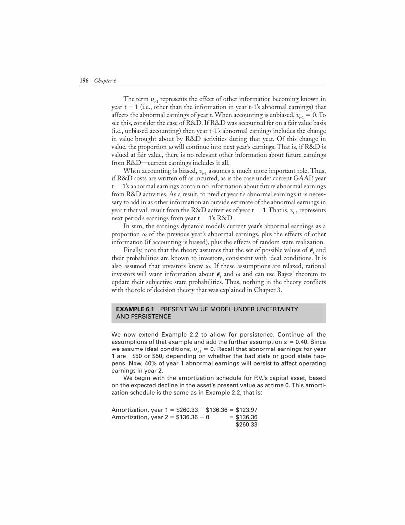
We now extend Example 2.2 to allow for persistence. Continue all theassumptions of that example and add the further assumption � � 0.40. Sincewe assume ideal conditions, �t-1 � 0. Recall that abnormal earnings for year1 are �$50 or $50, depending on whether the bad state or good state hap-pens. Now, 40% of year 1 abnormal earnings will persist to affect operatingearnings in year 2.

We begin with the amortization schedule for P.V.’s capital asset, basedon the expected decline in the asset’s present value as at time 0. This amorti-zation schedule is the same as in Example 2.2, that is:

Amortization, year 1 � $260.33 � $136.36 � $123.97Amortization, year 2 � $136.36 � 0 � $136.36

$260.33

196 Chapter 6

EXAMPLE 6.1 PRESENT VALUE MODEL UNDER UNCERTAINTY AND PERSISTENCE

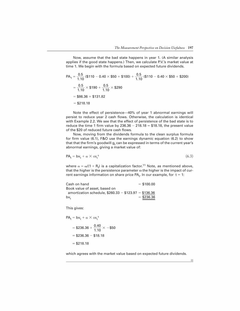
Now, assume that the bad state happens in year 1. (A similar analysisapplies if the good state happens.) Then, we calculate P.V.’s market value attime 1. We begin with the formula based on expected future dividends.

PA1 � �10.1.50

� ($110 � 0.40 � $50 � $100) � �10.1.50

� ($110 � 0.40 � $50 � $200)

� �10.1.50

� � $190 � �10.1.50

� � $290

� $86.36 � $131.82

� $218.18

Note the effect of persistence—40% of year 1 abnormal earnings willpersist to reduce year 2 cash flows. Otherwise, the calculation is identicalwith Example 2.2. We see that the effect of persistence of the bad state is toreduce the time 1 firm value by 236.36 � 218.18 � $18.18, the present valueof the $20 of reduced future cash flows.

Now, moving from the dividends formula to the clean surplus formulafor firm value (6.1), F&O use the earnings dynamic equation (6.2) to showthat that the firm’s goodwill gt can be expressed in terms of the current year’sabnormal earnings, giving a market value of:

PAt � bvt � � oxta (6.3)

where � �/(1 � Rf) is a capitalization factor.11 Note, as mentioned above,that the higher is the persistence parameter ω the higher is the impact of cur-rent earnings information on share price PAt. In our example, for t � 1:

Cash on hand � $100.00Book value of asset, based on amortization schedule, $260.33 � $123.97 � $136.36

bvt � $236.36

This gives:

PAt � bvt � � oxta

� $236.36 � �01..4100

� � �$50

� $236.36 � $18.18

� $218.18

which agrees with the market value based on expected future dividends.


The implications of the F&O model with persistence are twofold. First, evenunder ideal conditions, all the action is no longer on the balance sheet. The incomestatement is important too, because it reveals the current year’s abnormal earn-ings, 40% of which will persist into future periods. Thus, we can regard abnormalearnings as 40% persistent in this example.

Second, the formula (6.2) implies that investors will want information tohelp them assess persistent earnings, since these are important to the future per-formance of the firm. Our discussion of extraordinary items in Section 5.5showed how accountants can help in this regard by appropriate classification ofitems with low persistence. Also, the formula is consistent with the empiricalimpact of persistence on the ERC as outlined in Section 5.4.1, where we sawthat greater persistence is associated with stronger investor reaction to currentearnings.12

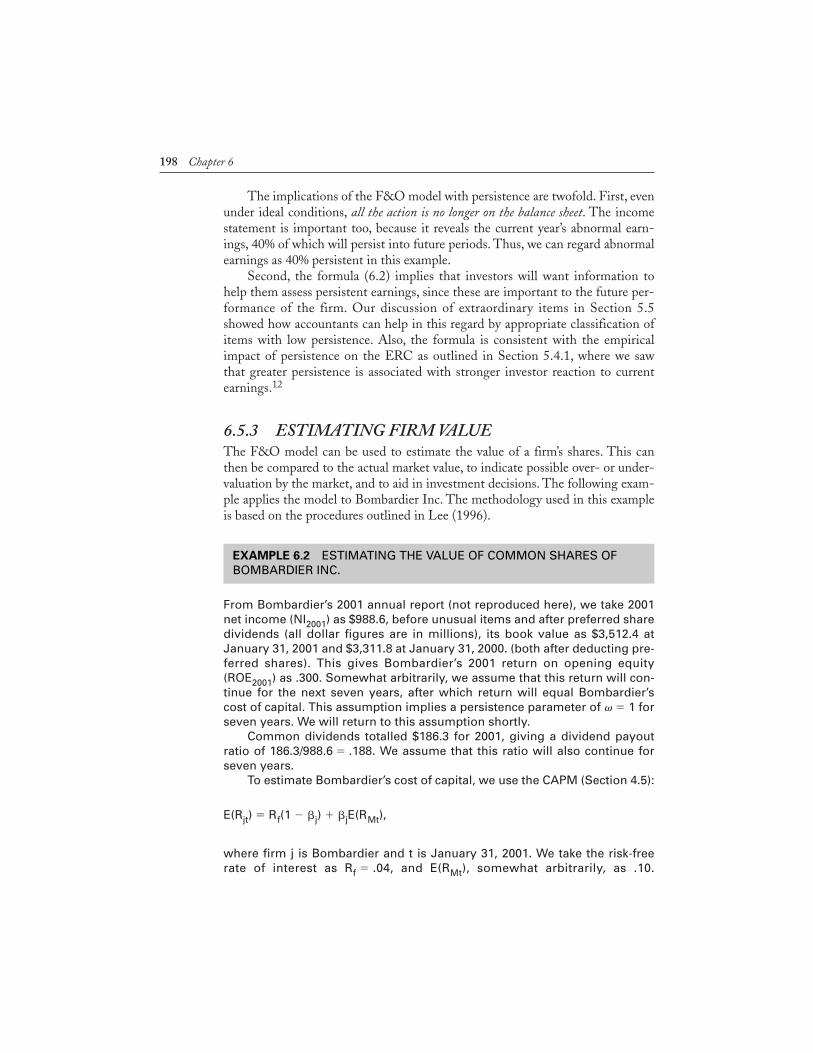
6.5.3 ESTIMATING FIRM VALUEThe F&O model can be used to estimate the value of a firm’s shares. This canthen be compared to the actual market value, to indicate possible over- or under-valuation by the market, and to aid in investment decisions. The following exam-ple applies the model to Bombardier Inc. The methodology used in this exampleis based on the procedures outlined in Lee (1996).

From Bombardier’s 2001 annual report (not reproduced here), we take 2001net income (NI2001) as $988.6, before unusual items and after preferred sharedividends (all dollar figures are in millions), its book value as $3,512.4 atJanuary 31, 2001 and $3,311.8 at January 31, 2000. (both after deducting pre-ferred shares). This gives Bombardier’s 2001 return on opening equity(ROE2001) as .300. Somewhat arbitrarily, we assume that this return will con-tinue for the next seven years, after which return will equal Bombardier’scost of capital. This assumption implies a persistence parameter of � � 1 forseven years. We will return to this assumption shortly.

Common dividends totalled $186.3 for 2001, giving a dividend payoutratio of 186.3/988.6 � .188. We assume that this ratio will also continue forseven years.

To estimate Bombardier’s cost of capital, we use the CAPM (Section 4.5):

E(Rjt) � Rf(1 � �j) � �jE(RMt),

where firm j is Bombardier and t is January 31, 2001. We take the risk-freerate of interest as Rf � .04, and E(RMt), somewhat arbitrarily, as .10.

198 Chapter 6

EXAMPLE 6.2 ESTIMATING THE VALUE OF COMMON SHARES OFBOMBARDIER INC.

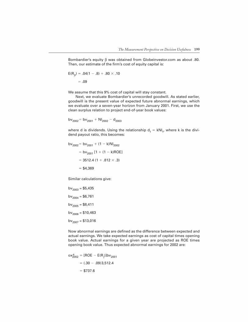
Bombardier’s equity β was obtained from Globeinvestor.com as about .80.Then, our estimate of the firm’s cost of equity capital is:

E(Rjt) � .04(1 � .8) � .80 � .10

� .09

We assume that this 9% cost of capital will stay constant.Next, we evaluate Bombardier’s unrecorded goodwill. As stated earlier,

goodwill is the present value of expected future abnormal earnings, whichwe evaluate over a seven-year horizon from January 2001. First, we use theclean surplus relation to project end-of-year book values:

bv2002� bv2001 � NI2002 � d2003

where d is dividends. Using the relationship dt � kNIt, where k is the divi-dend payout ratio, this becomes:

bv2002� bv2001 � (1 � k)NI2002

� bv2001 [1 � (1 � k)ROE]

� 3512.4 (1 � .812 � .3)

� $4,369

Similar calculations give:

bv2003 = $5,435

bv2004 = $6,761

bv2005 = $8,411

bv2006 = $10,463

bv2007 = $13,016

Now abnormal earnings are defined as the difference between expected andactual earnings. We take expected earnings as cost of capital times openingbook value. Actual earnings for a given year are projected as ROE timesopening book value. Thus expected abnormal earnings for 2002 are:

oxa2002 � [ROE � E(Rj)]bv2001

� (.30 � .09)3,512.4

� $737.6


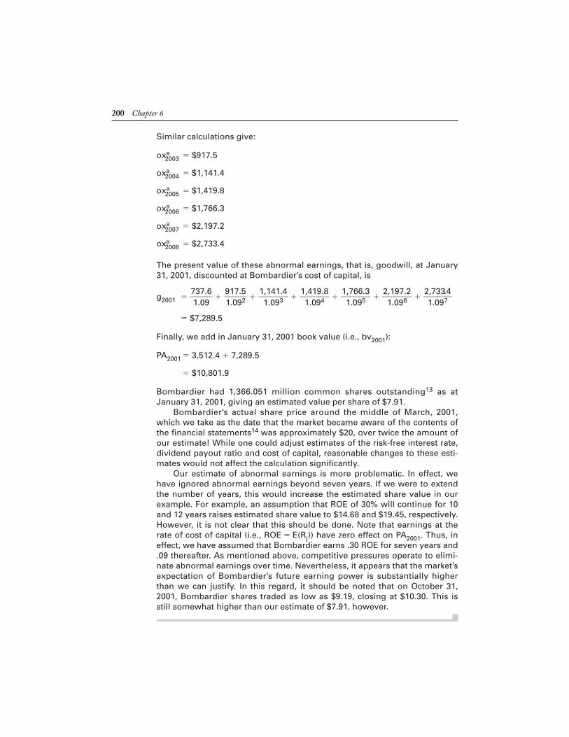
Similar calculations give:

oxa2003 � $917.5

oxa2004 � $1,141.4

oxa2005 � $1,419.8

oxa2006 � $1,766.3

oxa2007 � $2,197.2

oxa2008 � $2,733.4

The present value of these abnormal earnings, that is, goodwill, at January31, 2001, discounted at Bombardier’s cost of capital, is

g2001 � �713.079.6

� � �911.079.52� � �

11,1.0491

3.4

� � �11,4.0199

4.8

� � �11,7.0696

5.3

� � �21,1.0997

6.2

� � �21,7.03937.4

�

� $7,289.5

Finally, we add in January 31, 2001 book value (i.e., bv2001):

PA2001 � 3,512.4 � 7,289.5

� $10,801.9

Bombardier had 1,366.051 million common shares outstanding13 as atJanuary 31, 2001, giving an estimated value per share of $7.91.

Bombardier’s actual share price around the middle of March, 2001,which we take as the date that the market became aware of the contents ofthe financial statements14 was approximately $20, over twice the amount ofour estimate! While one could adjust estimates of the risk-free interest rate,dividend payout ratio and cost of capital, reasonable changes to these esti-mates would not affect the calculation significantly.

Our estimate of abnormal earnings is more problematic. In effect, wehave ignored abnormal earnings beyond seven years. If we were to extendthe number of years, this would increase the estimated share value in ourexample. For example, an assumption that ROE of 30% will continue for 10and 12 years raises estimated share value to $14.68 and $19.45, respectively.However, it is not clear that this should be done. Note that earnings at therate of cost of capital (i.e., ROE � E(Rj)) have zero effect on PA2001. Thus, ineffect, we have assumed that Bombardier earns .30 ROE for seven years and.09 thereafter. As mentioned above, competitive pressures operate to elimi-nate abnormal earnings over time. Nevertheless, it appears that the market’sexpectation of Bombardier’s future earning power is substantially higherthan we can justify. In this regard, it should be noted that on October 31,2001, Bombardier shares traded as low as $9.19, closing at $10.30. This isstill somewhat higher than our estimate of $7.91, however.

200 Chapter 6

Despite discrepancies such as this between estimated and actual share value,the F&O model can be useful for investment decision making. To see how, sup-pose that you carry out a similar analysis for another firm—call it Firm X—andobtain an estimated share value of $5. Which firm would you sooner invest in ifthey were both trading at $20? Bombardier may be the better choice, since it hasa higher ratio of model value to share value. That is, more of its share value is“backed up” by book value and expected abnormal earnings. Indeed, Frankel andLee (1998), who applied the methodology of Example 6.2 to a large sample ofU.S. firms during 1977–1992, found that the ratio of estimated market value toactual market value was a good predictor of share returns for two to three yearsinto the future. Thus, for the years following 2001, Frankel and Lee’s results sug-gest that Bombardier’s share return should outperform that of Firm X.

Nevertheless, the discrepancy between estimated and actual share price inExample 6.2 seems rather large. One possibility is that Bombardier’s shares areaffected by the momentum and bubble behaviour described in Sections 6.2.1 and6.2.5. Indeed, Dechow, Hutton, and Sloan (1999) (DHS), in a large sample ofU.S. firms over the period 1976–1995, present tentative evidence that investorsmay not fully anticipate the extent to which abnormal earnings decline over time.This evidence supports our refusal above to extend the period of abnormal earn-ings beyond seven years.

Another possibility, however, is that our estimate did not fully use all availableinformation. DHS also report that estimates of firm value based on the F&Omodel that ignored other information were too low, consistent with our results forBombardier. This brings us back to the υt-1 term in the earnings dynamic (6.2).Recall that this term represents additional information in year t � 1, beyond thatcontained in oxa

t � 1, that affects earnings in year t, and that it is non-zero whenaccounting is biased. Biased accounting is certainly the case. For example,Bombardier deducted R&D expenses of $123.4 millions in 2001. As you know,under GAAP, most R&D costs are written off in the year they are incurred, eventhough they may have significant impact on future earnings. To the extent thatR&D will increase future earnings, we may wish to increase our projected ROEabove 30% by adding back to reported earnings all or part of 2001 R&D expense.15

This would increase our estimate of share value. However, as a practical matter,estimating the future value of R&D is difficult, and we are reluctant to do this here.

Another source of additional information is analysts’ forecasts of earnings.Analysts will consider additional information in preparing their forecasts, not justthe information from current earnings as we did for Bombardier. If we had takenanalysts’ earnings forecasts into account in our estimates of future periods’ earn-ings, this may have improved our estimate of share price. Bombardier’s earningsper common share for 2001 were $0.70, and, from Globeinvestor.com in mid-July, 2001, the average analyst forecast of Bombardier’s earnings per share for2002 and 2003 are $0.90 and $1.14, respectively. Thus analysts are forecasting anincrease in earnings per share of 28.57% for 2002 and 26.67% for 2003, greater


than the (ROE � (1 � k) �) 24.36% increase implicit in Example 6.2. This sug-gests that we may wish to increase our estimate of Bombardier’s future profitabil-ity beyond 30% ROE. Supporting this suggestion, DHS report thatundervaluations of share price were reduced (but not eliminated) in their samplewhen analysts’ forecasts were included in their predictions. Nevertheless, in viewof the possibility of analyst optimistic bias pointed out in Section 5.4.3, we arehesitant to increase our estimate further.

We conclude that while our procedure to estimate Bombardier’s share price ison the right track, it may not have fully exploited all the financial statement andanalyst information that is available.This leads to an examination of empirical stud-ies of the ability of the clean surplus approach to predict earnings and share price.

6.5.4 EMPIRICAL STUDIES OF THE CLEAN SURPLUS MODEL

Clean surplus theory has generated much empirical research. One aspect of thisresearch compares the relative predictive ability of the dividend, cash flow andresidual income models. Recall from Section 6.5.1 that under ideal conditions allthree models produce identical valuations. However, when conditions are notideal, the model that produces the best predictions is an empirical matter. Forexample, it is often argued that the clean surplus model has an advantage becauseit uses balance sheet information and, as a result, has to project only abnormal orresidual income. Cash flow and dividend models must predict total future flows.Thus, the clean surplus model has “less” to predict and is thereby less subject toerror. It is also argued that the clean surplus model is more convenient to applythan the cash flow model. It uses readily-available financial statement informa-tion and does not have to back cash flows out of accrual accounting-based reports.

A major practical problem in applying all three models is the choice of fore-cast horizon, and what value, if any, to assign to flows beyond the horizon (calledthe terminal value problem). Our Bombardier estimate used a forecast horizon ofseven years, with a terminal value of zero on the grounds that competitive pres-sures are expected to eliminate abnormal returns beyond that time. Of course, thiszero terminal value assumption is rather arbitrary. Perhaps a better (but still arbi-trary) assumption is that Bombardier’s abnormal earnings would not fall to zero,but rather start to decline after seven years. Then, terminal value is greater thanzero, which would increase our value estimate.

An alternative assumption is to base terminal value on analysts’ long-rangeforecasts. In this regard, Courteau, Kao, and Richardson (2001), for a sample ofU.S. firms over the period 1992–1996, studied the relative predictive ability of thethree models, using analyst’s predictions of earnings in place of predictions fromthe earnings dynamic equation (6.2), and a five-year forecast horizon. They foundthat predictions using arbitrary terminal value assumptions, as we did forBombardier, substantially underestimated share market prices. When terminal

202 Chapter 6

values were based on analyst’s long-range forecasts, predictions were much moreaccurate. Furthermore, the three models were then roughly equal in their fore-casting ability, consistent with our theoretical expectation.

A second type of empirical clean surplus research studies the prediction offuture earnings, since future earnings are a main input into the goodwill estimate.In particular, this research examines how other information can improve earningsand share price predictions. This represents a significant change in emphasis fromresearch under the information perspective, which studies the association betweenfinancial statement information and share returns. As an example of this change inemphasis, consider the study of Abarbanell and Bushee (1997). In an extension ofthe approach used by Ou and Penman (1989) (Section 6.2.6) and Lev andThiagarajan (1993) (Section 5.4.1), they showed how certain “fundamental sig-nals” from the current financial statements, such as changes in sales, accountsreceivable, inventories, gross margin, and capital expenditure could improve theprediction of next year’s earnings changes. They went on to show that analystsappeared to underuse the fundamental signals when predicting earnings, suggest-ing that their earnings forecasts would benefit from greater attention to the fullinformation potential of financial statements. Myers (1999) adds order backlog asother information in the earnings dynamic, but finds this does not remove a ten-dency for under-prediction of firm value by the clean surplus model. Begley andFeltham (2002) add analysts’ forecasts and current capital expenditures as otherinformation. They find that these variables significantly improve prediction ofunrecorded goodwill for their sample firms. Overall, these results suggest consider-able promise for the usefulness of financial statement information, beyond theinformation in current earnings, in improving earnings and share price predictions.

A third type of research relates to the earnings dynamic itself. Instead ofusing the earnings dynamic to predict abnormal earnings, why not simply useanalysts’ earnings forecasts? These are readily available for up to five years ahead.Furthermore, despite the results of Abarbanell and Bushee (1997), outlinedabove, that analysts appear to underuse fundamental signals, they presumably usea large amount of other information, in addition to current earnings, whenpreparing their forecasts. As a result, the investor can be less concerned aboutwhat other information should be added in the earnings dynamic. Dechow,Hutton, and Sloan (1999), in their evaluation of different earnings predictionmodels, found that a simple projection of abnormal earnings based on analysts’one-year ahead earnings forecasts predicted share price as well as a full applicationof the earnings dynamic equation (6.2). Also, the study of Courteau, Kao, andRichardson (2001) referred to above uses analyst forecasts throughout. It seemsclear that the question of the best earnings prediction model, and the extent towhich accounting information is useful in this process, is unsettled.

Finally, another use of the theory is to estimate a firm’s cost of capital. InExample 6.2, note that any four of the five variables—share price, book value,expected future earnings, risk-free interest rate, and cost of capital—can be used,


in principle, to solve for the other one. This approach was used by Botosan(1997). In a study to be discussed in Section 12.3, Botosan used the clean surplusmodel to estimate the costs of capital of the firms in her sample, and then went onto demonstrate conditions under which high quality financial statement disclo-sure lowered cost of capital. Thus, the clean surplus model provides an alternativeto the CAPM for cost of capital estimation.

6.5.5 SUMMARYClean surplus theory has had a major impact on financial accounting theory andresearch. By demonstrating that firm value can equally well be expressed in termsof financial accounting variables as in terms of dividends or cash flows, it has led toincreased research attention to earnings prediction. Much of this research exploreshow current financial statement information can be used to improve this predic-tion. Better earnings prediction enables better estimates of unrecorded goodwill,leading to better predictions of firm value and hence better investment decisions.

The theory also leads to a measurement perspective, since the more fair val-ues are reported on the balance sheet the less the proportion of firm valueincluded in unrecorded goodwill, hence the less the potential for investor mis-takes in estimating this complex component of firm value. This can improveinvestor decision making and proper securities market operation, particularly ifsecurities markets are not as fully efficient as once believed.

6.6 Auditors’ Legal LiabilityPerhaps the main source of pressure in favour of the measurement perspective,however, comes as a reaction to spectacular failures of large firms, particularlyfinancial institutions. Many such failures have taken place in the United States. Forexample, an article in The Wall Street Journal (March 11, 1994, p. A2) reported thatResolution Trust Corp. had lawsuits against the audit firm of Deloitte and Touchetotalling $1.4 billion, and the Federal Deposit Insurance Corp. had lawsuits ofanother $450 million. The charges arose from alleged clean audit opinions issuedto savings and loan associations that, in retrospect, were insolvent. The articledescribes a proposed settlement of these lawsuits in excess of $300 million. Whileconsiderably less than the amounts at suit, this would still be the second-largestliability settlement surrounding the savings and loan debacle. (The largest was a$400-million settlement by Ernst and Young for similar charges.)

Under historical cost accounting, it can happen that firms that are here today,in the sense that their balance sheets and income statements show them to begoing concerns, are gone tomorrow. While accountants and auditors may claimthat information about impending failure was implicit in the notes or other

204 Chapter 6

sources, or was not their responsibility, there is a certain logic to questions raisedby those who ask why the financial statements proper did not more clearly foretellthe disaster. Auditors often have considerable difficulty in defending themselvesfrom the lawsuits that usually accompany business failure.

Furthermore, these legal liability pressures are likely to continue to increase.For example, Jensen (1993) points out that as technology advances, more andmore firms are finding themselves with substantial excess capacity. The resultingneed to downsize leads to mergers and acquisitions, reorganizations, layoffs, orbankruptcy. All of these events put severe pressure on the adequacy of historical-cost-based net income and asset valuation.

In addition, firms are facing increasing pressures to behave in socially andenvironmentally responsible ways. Many firms face substantial future liabilities inthis regard, for example in site restoration costs, which severely strain the conceptof matching costs and revenues.

One way that accountants and auditors can protect themselves against thesepressures is to adopt a measurement perspective, that is, introduce more fair valuesinto the accounts. Then, they can point out that the financial statements antici-pated the value changes leading to bankruptcy, merger, downsizing, environmentalliabilities, etc. Of course, this requires greater use of estimates and judgement but,because of legal liability, accountants may be more willing to adopt at least thosefair valuations that can be attained without substantial loss of reliability.

6.7 ConclusionsRecall that the information perspective on financial reporting is content to acceptthe historical cost basis of accounting, and rely on full disclosure to enhance use-fulness to investors. The form of disclosure does not matter, since it is assumedthat there are enough rational, informed investors to quickly and correctly incor-porate any reasonable form into the efficient market price. Empirical research hasconfirmed that the market finds net income information at least to be useful. Ineffect, empirical research under the information perspective tends to accept theefficient market price and to evaluate the usefulness of accounting information interms of its association with this market price.

However, there are a number of questions about the information perspective.First, securities markets may not be as fully efficient as had previously beenbelieved, suggesting that investors might need some help in figuring out the fullimplications of accounting information for future returns. Second, a “market share”of 2 to 5% for net income seems low and, despite theoretical support, it has beendifficult to find much direct market reaction at all to non-earnings accountinginformation. In addition, legal liability may force accountants to increase the use offair values in the financial statements. These questions are reinforced by the devel-


opment of the Ohlson clean surplus theory, which emphasizes the fundamentalrole of financial accounting information in determining firm value. This theoryimplies a more basic role for financial statements in reporting on firm value thanthe information perspective, which views accounting information as one of manyinformation sources competing for the attention of the efficient market. Thus, theclean surplus theory leads naturally to the measurement perspective.

Of course, for reasons of reliability, the measurement perspective would neverextend to a complete set of financial statements on a fair value basis. Historicalcost is unlikely to be displaced as the primary accounting basis for capital assets,for example. Rather, the question is one of degree—to what degree will fair valuessupplant costs in useful financial reporting? Consequently, in the next chapter wereview GAAP from a valuation perspective. There always has been a substantialpresent value and market value component to the financial statements. But, as weshall see, recent years have witnessed a number of new fair value standards.

Questions and Problems1. Why does a measurement perspective on decision usefulness suggest more

value-relevant information in the financial statements proper, when efficientsecurities market theory implies that financial statement notes or other disclo-sure would be just as useful?

2. What will be the impact on relevance, reliability and decision usefulness of finan-cial statement information as accountants adopt the measurement perspective?

3. Explain what “post-announcement drift” is. Why is this an anomaly for securi-ties market efficiency?

4. An investor considers two mutual funds. Based on past experience, the first fundhas expected return of .08 and standard deviation of .05. The second fund hasexpected return of .07 and standard deviation of .06. There is no reason toassume that future performance of these funds will differ from past perfor-mance. However, the second fund has a guarantee attached that return in anyyear will not be negative.

The investor buys the second fund. Use prospect theory to explain why.

5. Lev, in his article “On the Usefulness of Earnings” (1989), points out the lowability of reported net income to explain variations in security prices around thedate of release of earnings information. Lev attributes this low explanatorypower to low earnings quality.

Requireda. Define earnings quality. Relate your answer to the concept of an informa-

tion system in single-person decision theory.

206 Chapter 6

b. What other reasons might there be for the low explanatory power of earnings?c. How might an increased measurement perspective in financial statements

increase earnings quality, and hence the impact of earnings on security prices?

6. In Section 6.4, The concept of value relevance of net income is introduced. Itappears that the value relevance of reported earnings, as measured by R2 orERC, is low, and falling over time. Use single person decision theory to explainwhy value relevance of reported earnings can be measured by R2 or ERC.

7. On January 26, 1995, The Wall Street Journal reported that Compaq ComputerCorp. posted record 1994 fourth-quarter results. Despite $20.5 million in lossesfrom the December, 1993, Mexican currency devaluation, and losses on currencyhedging, earnings grew to $0.90 per share from $0.58 in the same quarter of1993, on a revenue growth of 48%. Furthermore, Compaq captured the No. 1market share spot, with shipments up 50% from 1993 and with slightly higherprofit margin.

Nevertheless, on the same day, Compaq’s share price fell by $5.00, a decline ofabout 12%. The Journal reported that analysts had been expecting earnings ofabout $0.95 per share. Also, there were concerns about Compaq’s scheduledintroduction of new products in March 1995, following a warning by Compaq’sCEO Eckhard Feiffer that first-quarter, 1995 earnings were likely to be “flat.”

Requireda. Use single-person decision theory and efficient securities market theory to

explain why the market price fell.b. Assume that the $20.5 million in losses from peso devaluation and currency

hedging are a provision, not a realized cash loss, at the end of the fourthquarter (i.e., an accrual). Use the anomalous securities market results ofSloan (1996) to explain why the market price fell.

c. The Journal quoted an analyst as stating “the market overreacted.” Useprospect theory to explain why the market might overreact to less-than-expected earnings news.

d. Which of the above three explanations for the fall in Compaq’s share pricedo you find most reasonable? Explain.

8. For what reasons might transactions costs, including investors’ time to figure outand operate strategies that appear to beat the market, not be a completely ade-quate explanation for the apparent efficient securities market anomalies?

9. Reproduced on page 208 is the Economic Value Added (EVA) disclosure fromthe MD&A section of the 1996 annual report of Domtar, Inc. Some of the usesof EVA are outlined in Domtar’s discussion in the disclosure. Of interest here isthe close relationship between the EVA measurement formula and the cleansurplus-based valuation procedure outlined in Example 6.2. Note that the EVA


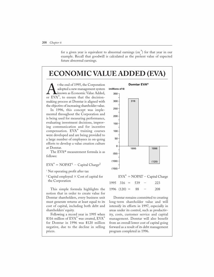
for a given year is equivalent to abnormal earnings (oxt

a) for that year in our

example. Recall that goodwill is calculated as the present value of expectedfuture abnormal earnings.

208 Chapter 6

ECONOMIC VALUE ADDED (EVA)

At the end of 1995, the Corporationadopted a new management systemknown as Economic Value Added,

or EVA®, to ensure that the decision-making process at Domtar is aligned withthe objective of increasing shareholder value.

In 1996, this concept was imple-mented throughout the Corporation andis being used for measuring performance,evaluating investment decisions, improv-ing communication and for incentivecompensation. EVA® training courseswere developed and are being provided toa large number of employees in on-goingefforts to develop a value creation cultureat Domtar.

The EVA® measurement formula is asfollows:

EVA® � NOPAT1 � Capital Charge2

1 Net operating profit after tax2 Capital employed � Cost of capital forthe Corporation

This simple formula highlights thenotion that in order to create value forDomtar shareholders, every business unitmust generate returns at least equal to itscost of capital, including both debt andshareholders’ equity.

Following a record year in 1995 when$316 million of EVA® was created, EVA®

for Domtar in 1996 was $120 millionnegative, due to the decline in sellingprices.

EVA® � NOPAT� Capital Charge

1995 316 � 539 � 223

1996 (120) � 88 � 208

Domtar remains committed to creatinglong-term shareholder value and willintensify its efforts in 1997, especially inareas under its control, such as productiv-ity, costs, customer service and capitalmanagement. Domtar will also benefitfrom an overall lower cost of capital goingforward as a result of its debt managementprogram completed in 1996.

01995

Domtar EVA®

(millions of $)

(50)

(100)

(150)

50

100

150

200

250

300

350

1996

(120)

316

Requireda. Evaluate the usefulness of this approach to communicating information to

investors. Consider both relevance and reliability issues.b. If you were the top manager of a company using EVA, would its use

encourage or discourage you from initiating major, capital intensive expan-sion projects? Explain why or why not.

c. You are an investor in a fast-growing, high-tech company that reports EVA.The assets of the company are primarily intangible (patents, skilled work-force), hence not included in the EVA capital charge. How would the largely intangible nature of the assets of such a company affect yourinterpretation of its EVA? Explain.

d. Note that reporting of EVA is voluntary. Domtar reports this informationfor 1996 even though its EVA is negative. Does Domtar’s willingness toreport this information add credibility to its claim that it “will intensify itsefforts in 1997?” Explain.

10. Recent years have seen considerable litigation against auditors in the UnitedStates, despite changes to litigation laws in 1995 that made it more difficult forinvestors to sue auditors.

A major source of this litigation arises from the pressure firms feel to meet ana-lysts’ earnings expectations. To avoid reporting lower-than-expected earnings,firms sometimes use earnings management, such as premature revenue recogni-tion and other devices, to raise reported net income. To avoid a qualified auditreport, the firm may pressure its auditor to “stretch” GAAP. This puts the audi-tor in a difficult position. If the auditor goes along, he or she will inevitably bedrawn into lawsuits when the earnings management becomes known (as it even-tually must, since accruals reverse).

For example, Waste Management Inc. overstated its earnings during a five-yearperiod in the 1990s, using a variety of earnings management devices such aslengthening the useful life of capital assets, increasing their estimated salvagevalue, and understating liabilities for rehabilitating contaminated waste dis-posal sites. In December, 1998, Waste Management’s auditor, ArthurAndersen, offered $220 millions to settle class action lawsuits following revela-tion of these practices.

One can sympathize with company managers for wanting to meet earningsexpectations. The market will severely penalize their stock price if they do not.For example, in 1997, Eastman Kodak announced that revenue would not meetexpectations due to the high value of the U.S. dollar, and analysts reduced theirestimate of first quarter, 1997, earnings from $0.90 per share to $0.80. Kodak’sshare price fell by $9.25 to $79 in heavy trading. Subsequently, Kodak reportedearnings per share for the quarter of $0.81, and share price rose $2.25 to $75.37.


This market reaction has been repeated many times since. An article in The WallStreet Journal in April, 2000 quoted a principal of Bogle InvestmentManagement as saying that the market is “overdiscounting” changes in earningsexpectations and that it is “reacting too much.”

Requireda. Why might an auditor be tempted to “cave in” to client pressure to manage

reported earnings so as to meet analysts’ expectations?b. To what extent would increased use of a measurement perspective in finan-

cial reporting reduce auditor exposure to client pressure and lawsuits?c. Use concepts from behavioural finance to explain why the market may

“overreact” to changes in earnings expectations.d. Is the $9.25 reduction in Kodak’s share price reported above inconsistent

with efficient securities market theory? Explain why or why not.

Notes1. It should be noted that Daniel and Titman’s investment strategy used hindsight

to pick stocks with high and low momentum. The strategy would not be imple-mentable in real time.

2. In mathematical terms, the utility function is continuous but not differentiableat zero.

3. Non-stationarity provides an alternative to noise trading, discussed in Section4.4.1, for the non-collapse of share prices on an efficient market. When shareprice parameters, such as beta, are non-stationary, investors will have differingopinions as to whether current share prices reflect their current beta values, andwill trade on the basis of these opinions.

4. For example, firms’ betas may shift when they announce good or bad earningsnews. If the beta shifts were positive for GN firms and negative for BN, thiscould explain post-announcement drift as simply an artifact of the higher (forGN firms) and lower (for BN) returns that investors would demand to compen-sate for the changes in risk, since, as discussed in Sections 3.4, 3.5, and 3.6,

210 Chapter 6

investors trade off risk and return. While BT present evidence that, followingearnings announcements, betas do shift in the manner described above, themagnitude of the shifts is much smaller than what would be required to explainthe magnitude of the post-announcement drift.

5. Suppose that transactions costs were 5% of the amount invested. Then, if it waspossible to gross 5% by a strategy of buying GN firms and selling short BNfirms, transactions costs would consume the 5% profit, so investors would notbother. Thus, what might appear to be a profitable investment strategy maymerely reflect the level of transactions costs required to earn those profits.

6. The proportion of variability is measured by the R2

statistic from the regressionof abnormal security returns on unexpected earnings.

7. The clean surplus model can be extended to allow for some information asym-metry, although under restrictive conditions. See Feltham and Ohlson (1996),reviewed in Section 11.6.

8. In the F&O model, the firm’s life is assumed infinite.

9. The “o” stands for “operating.” If the firm has financial assets, such as cash or secu-rities, these are assumed to earn the risk-free rate of interest. Consequently, financialassets do not contribute to goodwill, which is the ability to earn abnormal earnings.

10. The investor may wonder why the manager chose these particular accountingpolicies, however. That is, the manager’s choice of accounting policies may itselfreveal inside information to the market. Then, it is not completely correct to saythat the investor need not be concerned about accounting policy choice. This isconsidered in Chapter 11.

11. Our expression for differs slightly from that of F&O.They assume that the firmhas an infinite life, whereas our assumption is that P.V. Ltd. has a two-year life.

12. The persistence parameter � can be related to the three types of earnings eventsdistinguished by Ramakrishnan and Thomas (1991) (R&T) (Section 5.4.1),namely permanent, transitory, and price-irrelevant, with ERCs of (1 � Rf)/Rf ,1, and 0, respectively. First, consider a $1 permanent abnormal earnings eventoccurring in year t for a firm with an infinite life. This will increase bvt, in F&Onotation, by $1. In addition, � of this will persist to year t � 1, �2 to year t � 2,etc. Thus, the total effect, discounted at the rate Rf, of the $1 of year t abnormalearnings on PAt, that is, the ERC, is

ERC � 1 � �1 �

�

Rf� � �

(1 �

�2

Rf)2� � �

(1 �

�3

Rf)3� � …

� �1 �

1 �

Rf

R�

f

��


In R&T terms, permanent abnormal earnings have an ERC of (1 + Rf)/Rf. Toexpress this ERC in terms of ω, we have

�1 �

1 �

Rf

R�

f

��

1 �

Rf

Rf�,

which holds for � = 1.

Thus permanent abnormal earnings have � � 1. Note that this is outside therange of � in the earnings dynamic (6.2). That is, for an infinite firm horizonthe F&O model is not defined for permanent earnings.

R&T transitory abnormal earnings have an ERC of 1. Thus

�1 �

1 �

Rf

R�

f

�� 1,

which holds for � � 0. Thus, transitory earnings have an ω of zero.

For price-irrelevant abnormal earnings, with ERC of 0, we have

�1 �

1 �

Rf

R�

f

�� 0,

which is satisfied only in the limit as �→ ± ∞. Since this is again outside theallowed range for �, the F&O model is not defined for price-irrelevant abnor-mal earnings.

13. Bombardier Inc. has 2 classes of common shares outstanding—A & B. Theydiffer with respect to voting rights and dividend preference. However, theirmarket values and betas are almost identical. For purposes of this example, wecombine the 2 classes.

14. This is the date the financial statements for the year ended January 31, 2001were signed.

15. This is equivalent to adding in other information in the earnings dynamic equation 6.2.

212 Chapter 6

• • The Measurement Perspective on Decision … Measurement Perspective on Decision Usefulness 177 FIGURE 6.1 PROSPECT THEORY UTILITY FUNCTION U(x) x loss gain power) is likely

Documents