• Pawan Kumar Outline† Fast Radio Burst Physics & Cosmology

•

Pawan KumarOutline†

Paris, May 27, 2021

FRB physics – general constraints & a specific model

Fast Radio Burst Physics & Cosmology

• FRBs as probe of cosmology

†Wenbin Lu, Paz Beniamini (FRB physics)

• A brief summary of observations

M. Bhattacharya, E. Linder, X. Ma, Eliot Quataert (FRB-cosmology)

Fast Radio Bursts (FRBs)

The first FRB was discovered in 2007 – Parkes 64m radio telescope at 1.4 GHz

DM = 375 pc cm-3

Duration (δt) = 5msLorimer et al. (2007)

∴ Luminosity = 1043 erg s-1

(DM from the Galaxy 25 cm-3pc –– high galactic latitude)

Estimated distance ~ 500 Mpc

VEM = "#"$ ; signal at # is delayed, wrt # = ∞, by ∝ #)*

(from mean IGM density)

Dispersion relation for EM waves in plasma: #*=#+* + -*$* ; #+ : plasma frequency

(1010 times brighter than the Sun)

The magnitude of the delay is ∝ ./ = ∫1234-567489 ": ;5 (unit: pc cm-3)

Lorimer et al. (2007)

A Brief history (8 years of confusion and then a breakthrough)

16 more bursts detected (2010) in Parkes archival data by Bailes & Burke-Spolaor

These bursts were detected in all 13 beams of the telescope, i.e. most likely terrestrial in origin.

Clever detective work by Emily Petroff et al. (2015) established the origin of Perytons (microwave oven!)

Many people suspected that the Lorimer burst was also not cosmological.

Arecibo detects a burst in 2012; repeat activity found in 2015 (Spitler et al. 2016). Accurate localization led to distance measurement & confirmation that this event was cosmological and not catastrophic.

•

•

These bursts were dubbed Peryton – after the mythical winged stag.

FRB in our Galaxy! FRB200428

Figure 1: Time-series and dynamic spectrum of ST 200428A. We show dataobtained from the Owens Valley Radio Observatory (OVRO) alone. All data units aresignal to noise ratio (S/N). The quoted times are relative to the Earth-centre arrivaltime of the burst at infinite frequency. For a description of the data processing, see theMethods section. Top: De-dispersed time series of all available data on ST 200428A (seeMethods). The original data were de-dispersed at a DM of 332.702 pc cm�3. We detect noother radio bursts within our data, spanning a window of 131.072 ms centred on the timeof ST 200428A. We place an upper limit on bursts with S/N> 5 in this time window of< 400 kJy ms. Middle: Expanded plot of the region surrounding the burst. The relativearrival time of the second, brighter peak in the coincident X-ray burst (XP2) is indicatedas a vertical dashed line12,13. The full X-ray burst lasted approximately 1 s centred onUTC 14:34:24.444 (arrival time at the Earth center). Bottom: Dynamic spectrum of ST200428A corrected for the e↵ects of dispersion.

9

a

-15 0 15 30 45400

500

600

700

800

Freq

uenc

y(M

Hz)

0.0 0.2 0.4

0.0

0.2

0.4

0.6

0.8

1.0

Figure 1: Burst waterfalls. Total intensity normalized dynamic spectra and band-averaged time-series (referenced to the geocentre) of the detections by (a) CHIME/FRB and (b) ARO, rela-tive to the geocentric best-fit arrival time of the first sub-burst based on CHIME/FRB data. ForCHIME/FRB, the highest S/N beam detection is shown. Dynamic spectra are displayed at 0.98304-ms and 1.5625-MHz resolution, with intensity values capped at the 1st and 99th percentiles. Fre-quency channels masked due to radio frequency interference are replaced with the median valueof the off-burst region. The CHIME/FRB bursts show a “comb-like” spectral structure due to theirdetection in a beam sidelobe as well as dispersed spectral leakage that has an instrumental origin(see Methods).

8

CH

IME

And

erso

n et

al.

2020

STA

RE

-2(B

oche

nek

et a

l. 20

20)

Peak radio luminosity: 3x1038 erg s-1

Energy in radio bands: 2x1035 erg

It is associated with a well known magnetar (neutron star with super-strong magnetic field) with B=2.2x1014 G; P=3.2s

Energy in X-ray flare: 8x1039 erg (~0.2 s)[fxν α -0.6]

and spin-down age of 4x103 yrs

So, some FRBs are produced by magnetars!

Properties of FRBs (summary)

Duration:• 1 ms < tfrb < 20 ms~~

Flux variation time < 10 µs =) source region size < 105 Γ cm

•

The 9 localized FRBs do not show evidence for large local DM contributions

⇒

•

most FRBs are not associated with very young SN or dense regions of ISM.

Progenitor:

>500 FRBs have been detected of which >60 have repeat outbursts

Some bursts are 100% linearly polarized•

FRB radiation physics

How is the coherent radiation produced?

If the FRB radiation were to be incoherent, then the temperature of the object required to produce the observed luminosity should be

TB = F⌫d2Ac2

2(c�t)2⌫2kB> 1035k d2A28

!(x,t)

"# ∝ %

"# ∝ %&Which is unphysical.

∴ FRB radiation must be coherent

Photon occupation number, nγ = kB TB

h ν_____ ≈ 1037

Scattering probability is enhanced by the “occupation number” of the final state (nγ)�� �� �� ���

�� � ���

�� ��

�

For FRB radiation, nγ = kB TB

h ν_____ ≈ 1037

ωB = 1018 B12 Hz is cyclotron frequency and, and ω is FRB photon frequency

magnetic field is very strong and suppresses x-mode photon scatterings by a factor (ωB/ω)2 .

Plasma in the source region needs to be confined so that the enormous radiation pressure does not shut down the radiation process.

Photon beam size is small and scattering is not a problem.

R < 108 cm~ R > 1013 cm~

R ~ 1012 cm (E Γ n )

Radiation force due to induced Compton Scattering

(Because of cancellations, the effective cross-section is enhanced by a factor ~ 109 at R = 1013 cm ; declines with distance as R-3).

LOFAR 150 MHz data for 20180916 with L ~ 1041 erg/s is important as !"# ∝ % &'( & )"#*## ∝ %'+ &(

It is very hard to produce FRB radiation between ~108 cm & 1013 cm from the neutron star surface due to the enormous induced Compton force which quickly disperses the plasma.

Overview of shear wave → FRBLu, Kumar & Zhang, 2020

H~1 km

Crustal shear waves →Alfven wavesLu, Kumar & Zhang (2020)

vshear ~ 0.01 c

"shear ~ 104 Hz ~ vshear /H

Trapped fireball: Thompson & Duncan (1995) “standard” model for SGRs

H~1 km

Crustal shear waves →Alfven wavesLu, Kumar & Zhang (2020)

vshear ~ 0.01 c

"shear ~ 104 Hz ~ vshear /H

Predictions of the model

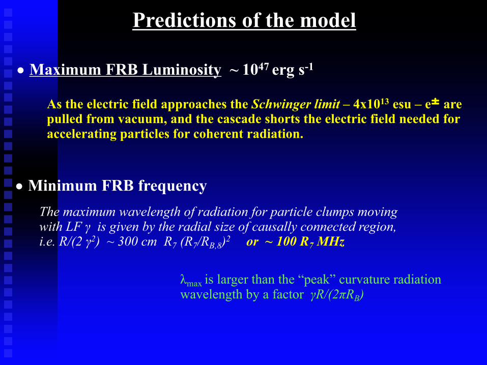
Maximum FRB Luminosity ~ 1047 erg s-1

As the electric field approaches the Schwinger limit – 4x1013 esu – e� are pulled from vacuum, and the cascade shorts the electric field needed for accelerating particles for coherent radiation.

•

• Minimum FRB frequencyThe maximum wavelength of radiation for particle clumps moving with LF γ is given by the radial size of causally connected region, i.e. R/(2 γ2) ~ 300 cm R7 (R7/RB,8)2 or ~ 100 R7 MHz

λmax is larger than the “peak” curvature radiation wavelength by a factor γR/(2πRB)

FRB cosmology

FRBs as probe of Intergalactic Medium

DM = Z

d`ne ⟹ Baryons in intergalactic medium (DM)

Map H & He-reionization epoch

DM

IGM

(cm

-3 p

c)

Macquart et al. (2020)

Ωb= ". "$%&"."'$("."'% )*"&%Sample size: 8 FRBs

Do we expect FRBs at high redshifts (z>6)?

Exploring the hydrogen reionization epoch using FRBs(Beniamini, Kumar, Ma & Quataert, 2021)

UV photons for the cosmic reionization (z>6) are supplied by stars ≥ "#$⊙

About &#% of massive stars produce magnetars at z=0 (Beniamini et al. 2019)

High z, metal poor, stars have faster rotation rates. They are likely to leave behind fast rotating compact remnants with strong magnetic fields as per the mechanism suggested by Thompson & Duncan.

In any case, we know that there are GRBs at z > 6, including one at 9.4 (Cucchiara et al. 2011).

GRBs require strong magnetic field & a compact object (BH or NS)

These high-z GRBs have properties similar to their lower-z cousins.

So, it is not a big stretch to assume that magnetars and FRBs should be there during the reionization epoch waiting to be discovered

••

•

•

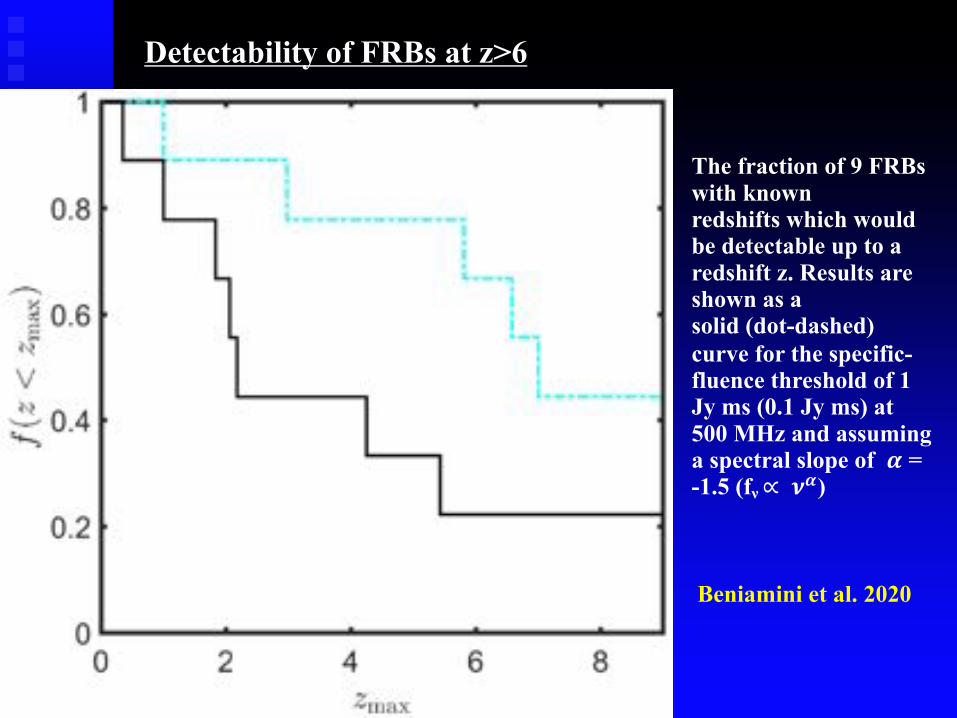
Detectability of FRBs at z>6

The fraction of 9 FRBs with knownredshifts which would be detectable up to a redshift z. Results are shown as asolid (dot-dashed) curve for the specific-fluence threshold of 1 Jy ms (0.1 Jy ms) at 500 MHz and assuming a spectral slope of ! = -1.5 (fν∝ #!)

Beniamini et al. 2020

Ocvick et al. (2021) courtesy of Shapiro

TIME

Cosmic Dawn II : Fully-Coupled Radiation-Hydrodynamics Simulation of Galaxy Formation and the Epoch of Reionization(“CoDa II”)

Blue regions are photo-heated, while small, bright red regions are heated by supernovae feedback and accretion shocks. The green color, on the other hand, denotes regions where ionization is ongoing and incomplete, and temperature has not yet risen to the ∼ 104 K typical of fully ionized regions. Brightness indicates the gas density contrast. Z=150 Z=5.8

Exploring Hydrogen Reionization Epoch

Beniamini, Kumar, Ma & Quataert (2021)H reionization with FRBs 3

Figure 1. The upper panel shows the number of electrons per baryon, ⇠e, asa function of redshift for two different H-reionization models. The solid linerepresents the current observational estimates for ⇠e at redshift larger than 6,cf. (Finkelstein et al. 2019; Robertson et al. 2015) which we refer to as ⇠e,o(z).The dotted curve (corresponding to ⇠e,t(z) which is given by Eq. 5) is a modelwe made up as a combination of linear and exponential functions to determinewhether FRBs can discriminate between different reionization histories. Thelower panel shows dispersion measure (DM) as a function of z for these twodifferent hydrogen reionization histories.

This expression for ⇠e for 3 < z < 4 approximately takes into ac-count the second helium reionization and above z = 6 accounts forthe first helium reionization and the hydrogen reionization. Note thatRobertson et al. (2015) provide ionization fraction for z & 6. At lowerredshifts we therefore adopt the same ionization histories for both⇠e,o(z) and ⇠e,t(z). We stress that the results in this paper are largelyindependent of the assumptions regarding the details of the HeII toHeIII reionization, as we are primarily interested at the distribution ofbursts at significantly higher redshifts/DMs. The purpose of the testmodel, ⇠e,t(z), is simply to demonstrate that the technique outlined inthis paper has the capacity to differentiate between different hydrogenreionization evolutions.

2.2 FRB rate and their DM distribution

2.2.1 The entire distribution

The number of FRBs in the local universe per unit volume, per unittime, with isotropic specific-energy2, E⌫0 , at frequency ⌫0 is found tobe a power-law function, e.g. Lu & Piro (2019)

f(> E⌫0) = �FRB E�↵E

⌫0,32, (6)

where �FRB ⇠ 1.1x103 Gpc�3 yr�1, ↵E = 0.7 and E⌫0,32 isthe isotropic equivalent specific-energy release by bursts at frequency⌫0 = 1 GHz in units of 1032 erg Hz�1. This power-law function holdsabove the minimum FRB energy E

min⌫0 ⇠ 1030 erg Hz�1 and below

Emax⌫0 ⇠ 1034 erg Hz�1. Note that we have assumed here that the

spectral energy distribution of FRBs is independent of redshift, whichis consistent with current observations (Hashimoto et al. 2020). Thisassumption can be easily relaxed if future observations, with muchlarger sample of FRBs (particularly those with known redshifts), sug-gest redshift evolution of FRB luminosity function.

We take the FRB rate per unit comoving-volume at redshift z tobe

nFRB(z,> E⌫) = f(> E⌫)n⇤(z)

n⇤(z = 0). (7)

where n⇤(z) is the number of stars formed per year at z with massin the appropriate range so that their remnants are neutron stars; weassume that the initial mass-function (IMF) is the same at low andhigh redshifts. The total mass of stars formed per comoving-volumeper year is taken to be as given by Madau & Dickinson (2014)

m⇤(z) = 0.015(1 + z)2.7

1 + [(1 + z)/2.9]5.6M� year�1 Mpc�3

. (8)

For a non-evolving IMF,

n⇤(z)n⇤(z = 0)

=m⇤(z)

m⇤(z = 0). (9)

The total number of FRBs per unit time (in observer frame) andper unit DM is

dNFRB

dDM=

nFRB(z, > E⌫)1 + z(DM)

4⇡r2(DM)dr

dDM, (10)

where we made use of the comoving volume at redshift z to be

dV = 4⇡r2dr =4⇡r2(z)cH(z)

dz, (11)

z(DM) is given by Eq. 4, r(DM) is comoving distance to an FRB atredshift z given by

r = c

Z z

0

dz

H=

c

H0⌦1/2m0

Z z

0

1

[(1 + z)3 + ⌦⇤0/⌦m0]1/2

, (12)

and the factor (1 + z) in the denominator of Eq. 10 converts the ratefrom comoving frame at z to the observer frame.

2.2.2 The observable distribution

The DM-distribution of FRB-rate above the observed specific fluenceeo,Th

⌫ is given by

dNFRB(> eo,Th

⌫ )dDM

=nFRB(z,> E

TH

⌫1 )

1 + z(DM)4⇡r2(DM)

dr

d(DM), (13)

2 Specific-energy refers to energy per unit frequency.

MNRAS 000, 000–000 (0000)

H reionization with FRBs 3

Figure 1. The upper panel shows the number of electrons per baryon, ⇠e, asa function of redshift for two different H-reionization models. The solid linerepresents the current observational estimates for ⇠e at redshift larger than 6,cf. (Finkelstein et al. 2019; Robertson et al. 2015) which we refer to as ⇠e,o(z).The dotted curve (corresponding to ⇠e,t(z) which is given by Eq. 5) is a modelwe made up as a combination of linear and exponential functions to determinewhether FRBs can discriminate between different reionization histories. Thelower panel shows dispersion measure (DM) as a function of z for these twodifferent hydrogen reionization histories.

This expression for ⇠e for 3 < z < 4 approximately takes into ac-count the second helium reionization and above z = 6 accounts forthe first helium reionization and the hydrogen reionization. Note thatRobertson et al. (2015) provide ionization fraction for z & 6. At lowerredshifts we therefore adopt the same ionization histories for both⇠e,o(z) and ⇠e,t(z). We stress that the results in this paper are largelyindependent of the assumptions regarding the details of the HeII toHeIII reionization, as we are primarily interested at the distribution ofbursts at significantly higher redshifts/DMs. The purpose of the testmodel, ⇠e,t(z), is simply to demonstrate that the technique outlined inthis paper has the capacity to differentiate between different hydrogenreionization evolutions.

2.2 FRB rate and their DM distribution

2.2.1 The entire distribution

The number of FRBs in the local universe per unit volume, per unittime, with isotropic specific-energy2, E⌫0 , at frequency ⌫0 is found tobe a power-law function, e.g. Lu & Piro (2019)

f(> E⌫0) = �FRB E�↵E

⌫0,32, (6)

where �FRB ⇠ 1.1x103 Gpc�3 yr�1, ↵E = 0.7 and E⌫0,32 isthe isotropic equivalent specific-energy release by bursts at frequency⌫0 = 1 GHz in units of 1032 erg Hz�1. This power-law function holdsabove the minimum FRB energy E

min⌫0 ⇠ 1030 erg Hz�1 and below

Emax⌫0 ⇠ 1034 erg Hz�1. Note that we have assumed here that the

spectral energy distribution of FRBs is independent of redshift, whichis consistent with current observations (Hashimoto et al. 2020). Thisassumption can be easily relaxed if future observations, with muchlarger sample of FRBs (particularly those with known redshifts), sug-gest redshift evolution of FRB luminosity function.

We take the FRB rate per unit comoving-volume at redshift z tobe

nFRB(z,> E⌫) = f(> E⌫)n⇤(z)

n⇤(z = 0). (7)

where n⇤(z) is the number of stars formed per year at z with massin the appropriate range so that their remnants are neutron stars; weassume that the initial mass-function (IMF) is the same at low andhigh redshifts. The total mass of stars formed per comoving-volumeper year is taken to be as given by Madau & Dickinson (2014)

m⇤(z) = 0.015(1 + z)2.7

1 + [(1 + z)/2.9]5.6M� year�1 Mpc�3

. (8)

For a non-evolving IMF,

n⇤(z)n⇤(z = 0)

=m⇤(z)

m⇤(z = 0). (9)

The total number of FRBs per unit time (in observer frame) andper unit DM is

dNFRB

dDM=

nFRB(z, > E⌫)1 + z(DM)

4⇡r2(DM)dr

dDM, (10)

where we made use of the comoving volume at redshift z to be

dV = 4⇡r2dr =4⇡r2(z)cH(z)

dz, (11)

z(DM) is given by Eq. 4, r(DM) is comoving distance to an FRB atredshift z given by

r = c

Z z

0

dz

H=

c

H0⌦1/2m0

Z z

0

1

[(1 + z)3 + ⌦⇤0/⌦m0]1/2

, (12)

and the factor (1 + z) in the denominator of Eq. 10 converts the ratefrom comoving frame at z to the observer frame.

2.2.2 The observable distribution

The DM-distribution of FRB-rate above the observed specific fluenceeo,Th

⌫ is given by

dNFRB(> eo,Th

⌫ )dDM

=nFRB(z,> E

TH

⌫1 )

1 + z(DM)4⇡r2(DM)

dr

d(DM), (13)

2 Specific-energy refers to energy per unit frequency.

MNRAS 000, 000–000 (0000)

Num

ber

of e

lect

rons

per

bar

yon

zz

He II reionization

H & He I reionization

DMmax depends on the reionization history

∆"#$%& = ()) *+ +$,- → ∆/0 ≤ ). ))3 (567768 79%: ;<%:+=)

Robertson et al. (2015)

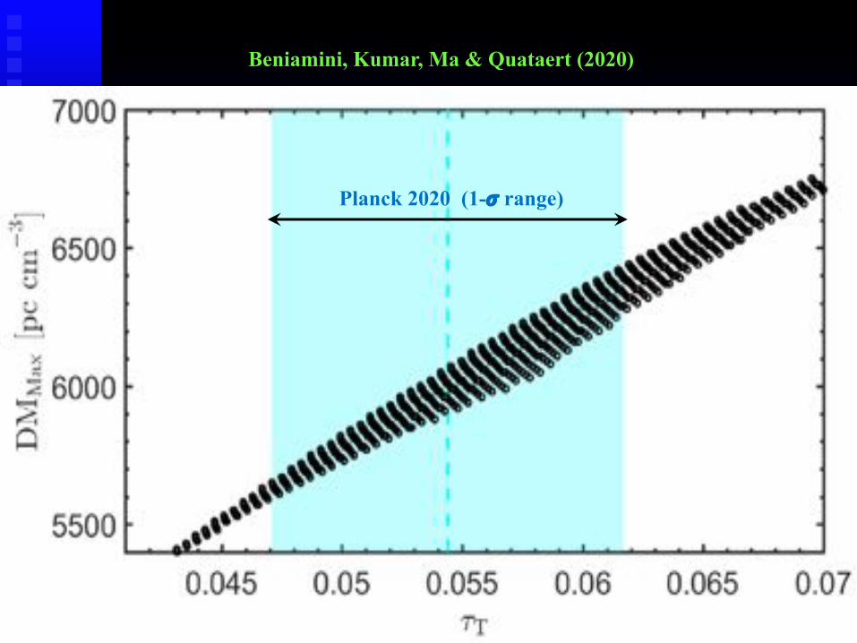
Beniamini, Kumar, Ma & Quataert (2020)

Planck 2020 (1-! range)

Beniamini, Kumar, Ma & Quataert (2020)

Planck 2020 (1-! range)

Num

ber

of e

lect

rons

per

bar

yon

Gray curves: reionization histories consistentwith Planck (2020) measurement of "#

Black curves: consisten with Planck (2020) & 5900 pc cm-3 < DM < 6100 pc cm-3

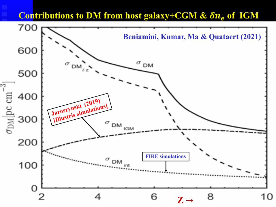
Contributions to DM from host galaxy+CGM & !"# of IGM

FIRE simulations

Jaroszynski (2019)

[Illustris simulations]

Beniamini, Kumar, Ma & Quataert (2021)

Z →

Exploring Hydrogen Reionization Epoch

Beniamini, Kumar, Ma & Quataert (2020)

10 Beniamini et al.

Figure 7. Top: Distribution of dNFRB/dDM resulting from a Monte Carlosimulation, with N = 105 detected FRBs, grouped in bins of constant width,�DM = 400 pc cm�3. The purple (cyan) error bars centered on dots (aster-isks) depicts 1� fluctuations about the mean value for the ionization fractionas described by ⇠e,o(z) (Robertson et al. 2015) (⇠e,t(z) defined in 5). Bot-tom: Deviations between the model using ⇠e,o(z) relative to ⇠e,t(z) (Eq. 5).The former model results in a relative excess of bursts with 5000 . DM .6000 pc cm�3 and a dearth of bursts with 6000 . DM . 7000 pc cm�3.The gray bars depict results with N = 104 detected bursts and the black withN = 105 detected bursts.

localization circle in the sky, and therefore the burst belongs in thesample for exploring the reionization epoch.

The measurement of redshifts and DMs for a small sub-sampleof FRBs would be very useful for determining how the average elec-tron density (per cc) in the IGM varies with redshift, nIGM(z), duringthe reionization epoch. This is facilitated by the fact that the contribu-tions to the DM from the FRB host galaxy and CGM is relatively small(see §3.1), and the contribution from our galaxy can be subtracted rea-sonably well. What’s more, determining ne(z) is more reliable fromDM(z) than it is using the Thomson scattering optical depth ⌧T(z), asthe latter quantity depends on the integral of electron density weighted

from further consideration for the purpose of investigating hydrogen reioniza-tion epoch.

Figure 8. Ratio of detected bursts with 6000 . DM . 7000 pc cm�3 andthose with 5000 . DM . 6000 pc cm�3, as a function of the total numberof detected bursts, N , for models with different re-ionization histories (purpleregion / solid line for ⇠e,o(z) (Robertson et al. 2015) and green region / dashedline for ⇠e,t(z) defined in Eq. 5).

by (1+z)2 – see Eq. 17 – whereas the DM integral has a weight factorof (1 + z).

Let us consider that redshifts of Ni FRBs are measured – fromtheir DMs, photometrically or spectroscopically – to be betweenzi ± �1i (in other words, 2�1i is the width of the bin around zi).The contributions to the DM of a burst at redshift z from IGM isDMIGM(z) ± �DMIGM

(z), and the host galaxy and the CGM isDMint(z)±�DMint

(z). Let us take the average error in redshift mea-surement at zi to be �2i. The variance of FRB-DMs for a large sampleof bursts due to their different redshifts, zi � �1i 6 z 6 zi + �1i, anderror in redshift measurements (±�2i), is given by

�DM�z

=dDMIGM

dz

⇥�2

1i + �2

2i

⇤1/2. (24)

Adding up the various contributions to the variance of FRB-DMsyields

�2

DM(z) = �

2

DMIGM

(z) + �2

DMint

(z) + �2

DM�z. (25)

The average DM for a sample of Ni FRBs can be written as

hDM(zi)i ⌘1Ni

NiX

j=1

DMj

= hDMIGM(zi)i+ hDMint(zi)i±�

DM(zi)

N1/2i

,

(26)

where hDMIGM(zi)i is the mean electron column density in the IGMupto redshift zi, and hDMinti is the average contribution to the DMfrom the FRB host galaxy and its CGM. We see in Fig. 6 that the con-tributions of the FRB host galaxy and the CGM to the total DM of anFRB, hDMinti, is of order 300 in the rest frame of the burst, whichis more or less independent of the FRB redshift. The hDMinti in theobserver frame is smaller by a factor (1 + z), and therefore for burstsat redshifts larger than 5 – the domain of exploration in this work –hDMint(zi)i < 102pc cm�3 or less than 2% of the total DM. Thevalue of �

DM(z) is plotted in Fig. 9. We see that �

DM

<⇠ 500pc cm�3

for z >⇠ 5. Therefore, to determine hDMIGMi at z = 5.5 with an ac-curacy of 2.5%, one needs to find ⇠ 20 FRBs within a redshift bin

MNRAS 000, 000–000 (0000)

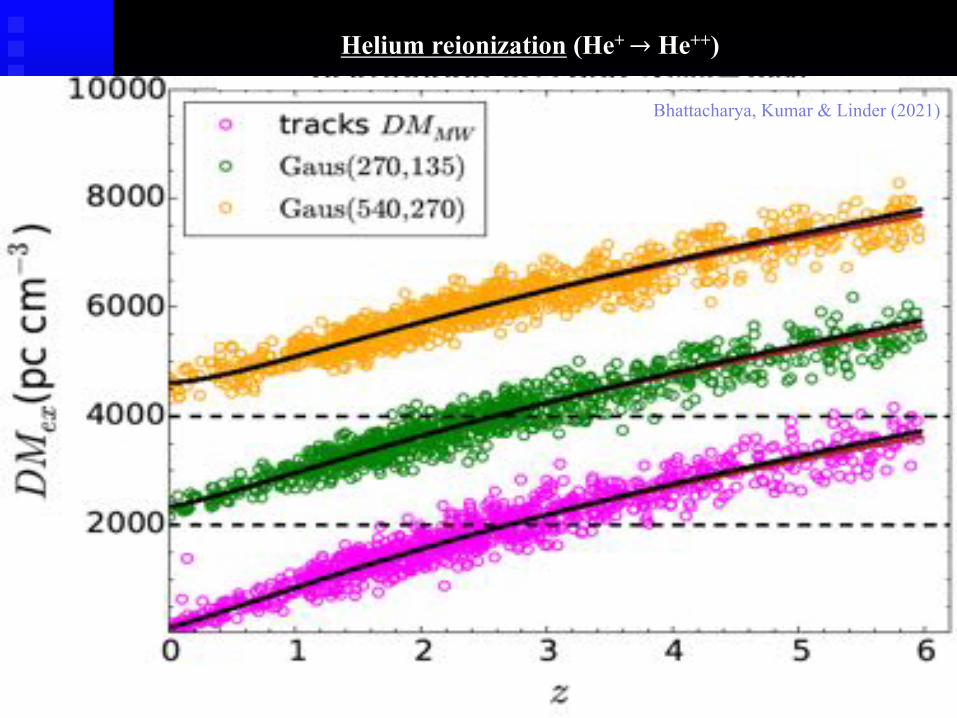
Helium reionization (He+ → He++)

Bhattacharya, Kumar & Linder (2021)

Summary

At least one FRB is associated with a neutron star with strong magnetic field (>1014 Gauss), probably all are.

•

FRBs seem promising for probing cosmology.•

Alfven waves launched from NS surface become charge starved at some radius. e� are accelerated in this process and produce FRBs via coherent curvature radiation mechanism.

•