. OCCASIONAL - World Fertility Survey

No. 17

L. KISH, R. M. GROVES . ·and ·K, P. KROTKI

Sampling Errors ' . for Fertility Survers

JANUARY 197p

. OCCASIONAL ,_ PAPERS ,

Managing Editor: Kay Evans

:INTERNATIONAL STATISTICAL INSTITUTE WORLD FERTILITY SURVEY Permanent Office • Director: R Lunenberg

· 428 Prinses Beatrixlaan Voorburg Netherlands

Project Director: Sfr Maurice Kendall, Sc. D., F.B.A. 35-37 Grosvenor Gardens London SWl W OBS

The World Fertility Survey is an international research programme whose purpose is to

assess the current state of human fertility throughout the world. This is being done principally

through promoting and supporting nationally representative, internationally comparable,

and scientifically designed and conducted &ample surveys of fertility behaviour in as many

countries as possible.

The WFS is being undertaken, with the collaboration of the United Nations, by the Inter­

national Statistical Institute in cooperation with the International Union for the Scientific

Study of Population. Financial support is provided principally by the United Nations Fund

for Population Activities and the United States Agency for International Development.

This publication is part of the WFS Publications Programme which includes the WFS Basic

Documentation, Occasional Papers and auxiliary publications. For further information on

the WFS, write to the Information Office, International Statistical Institute, 428 Prinses

Beatrixlaan, Voorburg, The Hague, Netherlands.

The views expressed in the Occasional Papers are solely the responsibility of the authors.

Sampli11g Errors for Fertility Surveys

Prepared by :

L. KISH, R. M. GROVES and K. P. KROTKI

Survey Research Center Institute for Social Research University of Michigan Ann Arbor, Michigan 48106 U.S.A.

ACKNOWLEDGEMENTS

The authors are grateful for support from the International Statistical Institute,

and from Mr. E. Lunenberg, Sir Maurice Kendall and Dr. J. T. Sprehe, and especially

for many helpful suggestions from Drs. C. Scott and V. Verma.

We are also grateful to several others who aided our search for data tapes and codes.

Those searches became our most arduous task, and the most often fruitless, because

of lack of available, adequate information that would allow the computations of

sampling errors (see Section 2.4).

Contents

FOREWORD

1 INTRODUCTION

2 METHODOLOGY 2.1 Portability: The Utility of Portable Measures of Sampling Variation 2.2 The Use of Roh and Deft for Imputation 2.3 Calculation of Roh Values 2.4 Formulas 2.5 Variability of Computed Sampling Errors and the Need for Averaging 2.6 Strategies for Sampling Error Computation

3 SUMMARY OF RESULTS FROM EIGHT SURVEYS 3.1 Introduction 3.2 South Korea Fertility Surveys (1971 and 1973) 3.3 Taiwan: General Fertility Survey (1973, KAP-4) 3.4 Malaysia: Survey of Acceptors of Family Planning (1969) 3.5 Peru: Urban and Rural Fertility and KAP Survey (1969) 3.6 United States Fertility Surveys (1955, 1960, 1965 and 1970)

REFERENCES

5

9

11 11 13 14 16 19 21

24 24 29 38 43 49 52

61

3

Foreword

Any survey which covers only part of the universe under inquiry is subject to a number of errors of different types. The so-called non-sampling errors (ii>accuracy of data, incomplete­ness of cover) exist, of course, in any inquiry, even a complete census, and may be just as important as the errors due to the sampling process. But they form a separate domain of study and are not dealt with in this note. In the absence of prior information, the optimal way of sampling is to choose members at random by some objective process, but unrestricted random sampling in a social survey has to be modified for theoretical and practical reasons, of which the two main ones are:

1) By stratification. If the population under study can be divided into strata, e.g., by geographical area or by ethnic groups, it may be convenient to allocate the total sample proportionately to the various strata, or even disproportionately if some strata are more heterogeneous or require greater accuracy or more intensive study than others.

2) By clustering. To economize in travel time, sub-areas may be selected from a main area and the individual members chosen from within each selected sub-area.

The sampling plan for each survey has to be designed ad hoc, in the light of various factors, such as what is already known about the population under study (the sampling frame, the availability of maps, the accessibility of certain areas), the amount of staff available for field work and the over-all cost. This leads to the concept of the Design Effect or Design Efficiency Factor ( deff) which tries to measure the relative efficiency of the design as compared with what it would have been had the sample been selected entirely at random. Efficiency in this sense is measured by sampling variance, that is to say, the square of the standard error (ste). This basic statistical concept sets probabilistic limits to the amount by which the parent value under estimate differs from the observed value in the sample. Under certain conditions, the variance can be calculated a priori on theoretical grounds; in other cases, it has to be estimated from the data themselves. A common and convenient criterion asserts that the true value lies within a range of twice the standard error on either side of the sample value. The object of a good design is to reduce this standard error as much as possible. If comparisons are made between standard errors instead of variances the corresponding ratio is denoted by deft. It is the square root of the deff. However, each variable has its own standard error and consequently the deff is not an absolute single quantity attached to the design, but is a set of quantities, one for each variable under estimate. One may legitimately speak of the deff for variable x or variable y but not of the def! of the whole design unless (a point reverted to below) it is possible to amal­gamate the deff's for all the variables of interest into a single index number expressive of

5

the average deff over all the variables. The main factor affecting the design efficiency is the effect of clustering. If, among the group forming the cluster, there are correlations of appreciable size, the amount of information from a set of n individuals is not n times the amount of information derived from one indi­vidual. In practice one may expect some positive correlation between neighbouring members in a cluster and this reduces the efficiency of the sampling. The central point of interest is how much the efficiency is reduced, considered as a trade-off against the saving in expense achieved by clustering the sample. A measure of the degree of relation between the members of a cluster is the so-called intra­class correlation, which is a kind of average of the correlation among them and is usually denoted by the Greek letter rho, (]. Consider the sum of a number of variables x 1 to x 11 , all or some of which may be correlated. Its variance is given by

var (Sum) = I: var xi + i=1

~ COY (xi, xj). i*j

If the variances of xi are all equal then

var (Sum) = n + n (n - 1) Q

var xi

where Q is the average correlation among the x's. Thus

var (Sum) "" = 1 + (n - 1) Q.

n ""'var X;

The expression on the left is the deff of this particular cluster and hence

deff - 1 (] =

II - 1 •

Where a whole design is under consideration, comprising various clusters, Kish and his colleagues take an average of the cluster size and write

deff - 1 rah=-,---

b-1

where b is the average size. The deff is calculated from the data by formulae set out in the text and hence roh is computed. Kish et al use roh instead of the more familiar rho to remind the reader that it is an average of intraclass correlations and ex post facto identified in the letters with the initials of Rate of Homogeneity. If there is no intraclass correlation roh is zero and the deff is unity. Theoretically roh can attain unity, in which case the deff will be high (an inefficient design, as is otherwise obvious from the fact that all the members

6

within a cluster give identical answers to the variable concerned). In practice values of roh between zero and 0.2 can be expected. In the following monograph the authors have worked out the standard errors and the corresponding deft and roh for a large number of variables in eight different surveys from five countries and a glance at their tables will illustrate the kind of numerical results which emerge. One useful consequence of this kind of study is that it may be possible to extrapolate from existing analysis to estimate beforehand what the deff of a new design is likely to be. For this reason the authors recommend estimating the value of roh rather than the deff itself because the latter depends on the cluster sizes whereas roh is relatively insensitive to them. This is what the authors mean by saying that roh is 'portable'. Although, as they point out, complete portability is not achievable, it is, nevertheless, a very useful guide to the efficiency which is likely to be attained and enables different designs to be compared in advance. It is also of interest to compare, for any one design, the efficiency of different variables or groups of variables. The tables in the monograph for example, confirm the impression that socio-economic variables have larger standard errors and greater intraclass correlation than some of the demographic variables. Finally the authors give data on the design efficiency within subclasses of the population and for differences between pairs of variables. These results relate more closely to real-life appli­cations of the survey findings. It is an open question whether the deffs obtained from individual variables can be amal­gamated into a single index to give some idea of the deff as a whole. A good deal, of course, depends on which variables enter into such an index, just as a cost-of-living index depends on the basket of goods which compose it. It seems unlikely that different types of survey can be compared in such a summary manner; but perhaps an index could be constructed for surveys of a similar kind.

Sir Maul'ice Kendall Project Director, WFS

November 1975

7

1. Introduction

This investigation is based on eight fertility surveys from 5 countries: South Korea, Taiwan, Malaysia, Peru and the United States, all of them conducted before the World Fertility Survey was begun. For each survey we computed sampling errors on about 30 to 40 different variables. For each variable sampling errors were computed for means or proportions based on the entire sample, also for about 24 diverse subclasses (domains of study), and for differ­ences (comparisons) between about 12 pairs of those subclasses. Thus for each survey a total of about (30 to 40) x (1 + 24 + 12), or about 1000 to 1600, sampling errors were computed. Each of the calculations of sampling errors included not only the variances and standard errors, but also 'design effects' and intraclass correlations. These were analyzed to search fo1• stable and useful relationships among them. The entire investigation has two broad goals. First, our data on sampling errors and relation­ships should guide the designs of similar samples in other countries. Immediately, we are concerned with the World Fertility Survey, but the results are general enough to be useful for many other kinds of surveys. Second, we suggest methods for the calculation, analysis and presentation of sampling errors from future surveys. Our presentations and justifications provide some implicit guidance, and we add some explicit suggestions. For both goals we try to create guidelines for imputing values from computed sampling errors to unknown sampling errors. It is not feasible to compute, even less so to present, sampling errors individually for means of all variables, much less for all subclasses, and especially for all comparisons of subclasses. Our guidelines for imputation utilize some empirically estimated relationships, linking sampling errors on the total sample to those on subclasses, and then linking these to the differences of subclass means. We also suggest techniques of imputation across different variables within types for single surveys, as well as for similar variables across different samples. From the computed variances we construct measures that greatly facilitate the process of imputation: design effects and measures of intraclass correlations. The design effect is defined as the ratio of the actual sampling variance, taking into account the complexity of the sampling design, to the variance of the same sample size (n) under assumptions of simple random sampling [Kish, 1965, 8.2]. We use the symbol def!, but more often its square root, deft = . .j def!, which is the ratio of standard errors. Thus deft 2 = dejf =

computed variance/srs variance. For subclasses of diverse sizes we computed values of syn­thetic intraclass correlations; these values of rah measure the degree to which values for variables are homogeneous within sample clusters. We compute roh = (deff - 1) / (b - 1), where b is the average size of sample clusters. Randomly distributed variables have roh

9

values near zero, whereas highly clustered items are found near 0.10 or 0.20, and perfectly segregated variables can theoretically approach 1.0. Thus we propose the following indirect method of imputation from a computed standard error (ste0) to an unknown one (ste1):

computed ste0 imputed ste1

t deft0

t roh 0 imputation roh1 »- - - - - - - - - -l>

We impute across roh values because of their relative stability across diverse subclasses for each variable from a sample, and also for similar variables across samples. We transform values of ste into deft, and these into roh; then, after imputing roh for a new statistic, we transform into the new deft, and finally to the needed ste. The direct imputation from ste 0

to ste1 is seldom justified. The path from deft 0 to deft1 is usually difficult also, due to large differences in sample sizes, hence cluster sizes, for diverse subclasses.

We devised some approximate methods to further our two stated aims. Some of these methods emerged after several false starts; these also caused differences in the presentations of the several sets of data. Though we had computed many sampling errors over the years, the volume and diversity oT these data presented new challenges and opportunities. Our methods are subject to further developments and modifications, and we invite participation and suggestions. The remainder of this report is divided into two sections. The first clarifies the need for portable measures of sampling variation for use in imputing from computed variances to unknown values for other statistics and for different designs; describes the use of the synthetic intra­class correlation, roh, for such imputations; describes calculation procedures for roh for subclasses and for subclass comparisons; presents formulas for sampling errors; describes the variability in computed sampling errors and justifies our use of averages over variables and subclasses; and suggests strategies for the calculation and presentation of sampling errors of future samples. The second section presents and discusses our empirical results from eight fertility surveys.

10

2. Methodology

2.1 PORTABILITY: THE UTILITY OF PORTABLE MEASURES OF SAMPLING VARIATION

We aim mostly to compute and present estimates of design parameters that can be used both simply and generally for diverse multipurpose designs. Simplicity and broad utility are our goals, for which some compromises in precision have been made. Words that first come to mind are generality, invariance and robustness. However, these carry with them more or less special connotations; we prefer to avoid the confusions and arguments that would result from a somewhat different use of these accepted terms. We think that portable and portability convey the meaning we need. Portability refers to properties of the estimate that facilitate its use far from its source. To illustrate, let us begin with the standard errors, ste (y), one computes for making in­ferential statements like y ± tP ste (y). Standard errors computed for one statistic can be imputed directly only to essentially similar statistics based on similar subclass sizes from similar survey designs. They are specific to the estimate y and depend on:

a) the nature of the variables, b) their units of measurement, c) the nature and design of statistics derived from the variables, d) size of the sample bases, which can vary greatly for subclasses, e) sizes of selections from sample clusters, and f) nature and size of sampling units.

Design effects are considerably more portable than standard errors. They are widely used to modify simple random estimates stesrs (.Y) to guess at some ste (y) as deft x stesrs (y). When we compute deft (y) = ste (51) / stesrs (y), we remove the scaling effects of the units of measurement and of the sample's aggregate size. We prefer to use deft rather than coeffi­cients of variation ste (Y)/y; these are unambiguous only for positive quantitative variables, they remove the effects of units of measurement but depend on sample size. We may sometimes assume that deft0 = deft1 , where the subscripts denote different variables. This would usually serve better than would assuming either that ste1 = ste0 or that ste1 =

ste srs. However, the assumption can also be misused, and the portability of defts has been naively overestimated by many. First, within the same survey many statistics are based on subclasses, whose sizes vary greatly. If deft 0 is computed from the entire sample, the deft1 for the same variable on a subclass is often considerably smaller. Design effects for most sub­classes diminish along with sample size; and using values of deft computed from the entire

11

sample grossly exaggerates the actual effects of the design on subclasses. Second, deft values depend heavily on the sizes of sample clusters used, which may differ drastically from one survey sample to another. The design effect may be expressed as a function of two components:

1) the degree of homogeneity within sample clusters measured by the intraclass corre­lation (roh); and

2) the number of elements in sample clusters (li).

Since deft 2 = 1 + roh (li-1), as the size of the sample cluster increases (for larger subclasses, or for new samples with larger clusters) for any variable, its deft 2 tends to increase also. We need portability to make inferences from one set of results to another set of variates with diverse values of li in the same survey or for designing another survey. Values of roh are more portable for this purpose than deft or than standard errors. The computed values of roh are functions of the kind of sampling units used and the nature of the selection process. However, we found usable stable relationships of rohs for subclass means to rohs for total sample means, much more stable than for values of deft or of ste. For the sake of portability we had to make some heroic simplifications. The relationship deft 2 = 1 + e (b - 1), where e is the intraclass correlation, is clearly defined for random subsampling of equal clusters b in two stages. However, most samples have further compli­cations: several selection stages, stratifications for each stage, unequal sizes of clusters, and diversity of selection methods in different parts of the sample. To compute all the compo­nents of the design would be difficult for individual statistics. Moreover, it seems impossible to present and to utilize such detail for many (1000 or more) statistics. We define the computed values of deft 2 to incorporate and carry the full complexity of the design used to obtain the average cluster sizes li. We then define roh as the portable parameter, relatively constant for a variable for diverse subclasses from one sample design. The precision in values of roh that we sacrifice are often within 10 or 20 per cent, seldom as great as a factor of 2, we think. On the contrary, the range of roh values for diverse variables within each survey are seen to vary by factors of 100. Nevertheless, we must remain aware of factors that interfere with complete portability. First, the computed values of roh are also functions of the kind of sampling units used and of the selection procedures in several stages. These effects need to be judged from descriptions of the sample design; it would be impractical to try to estimate, present and utilize all of the variance components for many variables. But these problems of using roh appear minor compared to great differences in roh values found for diverse variables from the same survey. We found usefully stable and portable relationships of rohs for diverse subclass means to rohs for total sample means much more so than for values of deft or of ste. Second, the sizes of sample clusters lido not decrease in perfect proportion to subclass sizes; proportionality is roughly approximated only by cross-classes, as discussed in the next section.

12

2.2 THE USE OF ROH AND DEFT FOR IMPUTATION

Basically, we need to make imputations from computed standard errors (ste0) to unknown standard errors (ste1) of other variates. Design effects are often more portable than standard errors, and are used to impute from computed ste0 = [a 0 / .Jn0 ] deft 0 to unknown ste1 = [a1 I .J111] deft1. At times we may assume that deft 0 = deft1 approximately, even when a1and111 differ notice­ably from a0 and 11 0 • This may seem reasonable for similar statistics from the same survey, or from similar surveys. However, the stability of similar deft values often appears weak, especially when the sample bases differ. Then imputing a different deft1 value from deft 0

cannot be done well directly, and we resort to values of roh for imputation. We must first impute some value roh1 = Jc1roh0 from computed values of roh 0 and from an imputed factor A1. Then we estimate the unknown deft1 from

We estimate the size of sample clusters b1 from b1 = 111/a from the size of the sample base 111, and from the number a of primary clusters. Imputing Jc1 becomes the chief task, and must rely on judgment based on studies of empirical data. We may guess that roh1 = roh0 and Jc1 = 1 roughly, for similar variates based on similar types of subclasses. Or we may guess some value J,1 =fa 1 in many situations. We found some usefully stable relationships of roh, and present them later. As a rough average we find Jes = rohs/roh1 ,....., 1.2, with roh1 for the entire sample and rohs as an overall average for subclasses. Then if the proportion of a subclass is Ms in the sample (and the population), we may impute for the subclass mean the unknown <lefts

deft.2 = [1 + rohs (bs -1)] = [l + 1.2 roh1 (b1Ms - l)].

For example, assume we had deft( = 5.9 for a variable and cluster size b1 = 50 from the entire sample. Then roh1 = 0.10 is estimated from deft;= [l + roh1 (50-1)] = 5.9. Hence for subclasses of proportion Ms = 0.2 of the entire sample we impute deft; = [l + 1.2 (0.10) (50 x 0.2 - l)] = 2.08. For a smaller subclass of Ms = 0.1 the deft; = 1.48. For another variable with roh1 = 0.01 the three deft; would be much smaller: 1.49, 1.11 and 1.05. Small errors in choosing precise values for J, are much less important than the effects of iarge variations in roh across variables, and in subclass sizes Ms. This will be seen later in our empirical results. We need to impute values of rohs for subclasses, from values roh1 computed for the entire sample, or for similar type subclasses. Thus we need stability (portability) for roh values, and we seem to find that for cross-classes. This type seems to cover many, probably most, subclasses used in survey analysis: such as subclasses by age, sex, income, education, most occupations, attitudes, behaviour, etc. Briefly, cross-classes is a term we coined for subclasses

13

that cut across the clusters and the strata used in the selection process: so that the sizes of sample clusters for each subclass are roughly b8 = btMs> where lvl8 is the proportion of the subclass in the sample (and population) and bt is the average cluster size for the entire sample (when Ms = 1). Not all subclasses are cross-classes. At the other extreme are subclasses that follow the lines of the primary divisions (PSUs, strata) of the population in the sample design. Examples in most samples are regions, also city size and rural subclasses that sort entire primary units into subclasses. For these segregated classes we would expect deft to remain roughly constant, and not to vary in proportion to the size of the subclass. We assume for these that deft 2 =

[I + roh (b - l)] remains constant because the sizes b and the roh values are roughly similar in the segregated classes. But in some samples, b (01 roh) may be entirely different in different portions of the design, and the values of deft 2 can differ greatly (see Malaysia, Section 3 .4). In our experience most of the commonly used subclasses tend toward cross-classes; but some segregated classes can be easily identified. Relatively few fall in between the two extreme types; examples are national or ethnic groups that are strongly segregated, but not so much that they were made strata or complete clusters in the design.

2.3 CALCULATION OF ROH VALUES

Values of the design effects deft 2 = var (Y) / (a2/11) for means can be readily computed and built into computing programs. These are overall values for the entire sample design, and they incorporate several design features, including both clustering and stratification. This also holds for means of subclasses which are not too small or restricted. The estimates of a2/n can be estimated readily for epsem (equal probability of selection per element) designs, and even more easily as pq/n for proportions p, which occupy much of survey analysis. It has been shown that s2 is a nearly unbiased estimate of a 2 in complex but large samples [Kish, 1965, Section 2.8]. However, we need to go from deft to roh, using deft 2 = [1 + roh (E - 1) ]. We use b = n/a where n is the number of elements (in self-weighting samples) and a is the number of primary selections. To the extent that the sizes of sample clusters vary around b, our computed syn­thetic roh wili tend to overestimate the correlation in the populaiion. Bui this overestimation is slight in most cases, when the cluster sizes do not vary wildly. Furthermore, for portability we prefer our synthetic roh to include the overestimation, so that we may use it directly for different subclass bases, with diverse cluster sizes b8 • We deal here with cross-classes that are spread widely, more or less randomly, across most of the primary units. There is relatively greater variation in cluster sizes for subclasses than for the entire sample, though for larger subclasses this may still not be too serious. We compute the rohs value for subclasses (s) from defV = [1 + rohs (b8 -1) ].

14

We must face another difficulty when we need to compute average values of roh =

(deft 2 - 1)/(b - 1) for designs in which the cluster sizes are vastly different between major divisions. For example, primary selections averaging 50 to 100 interviews per district may be taken in rural areas, but clusters of size 2 (per block) or even 1 (direct element selection from a list) in the big cities. Here separate deft values for the urban and rural divisions should be computed; see the sample from Malaysia (Section 3.4). Yet we also need to present average roh values, especially for subclasses, like age or education, which cut across the divisions. For this purpose we devise a synthetic cluster size b = n/a, with a synthetic number a of primary selections. Suppose that the relative sizes of the divisions of the population are measured by W; = n;fn, with I:W; = 1. (This supposes a self-weighting sample; drastic departures from this may need separate consideration.) Then the synthetic values for a and b can be found from the a; primary selections in the divisions:

1 W; 2 1 11; 2 - 11 II; 11; - = ~ - = 2 I: - and b = - = ~ - · - · a ~ 11 ~ a 11 ~

We found an extreme situation in the survey of Malaysia with the sample divided into two strata ( i = 1, 2), with large clusters in the rural stratum and with element sampling (a2 = 112)

in the urban stratum; thus

11 111 111 112 112 111 111 112 -=-·-+-·-=-·-+-a 11 a1 n a2 11 a1 n

In Table 11 (Malaysia), the average value of roh = 0.0463 for the rural base in Column 2 is seen to be reflected accurately by the average value of synthetic roh = 0.0453 in column 3. We know that this computed roh value is a synthetic average, and the separate roh values within the divisions may well diverge widely from the synthetic average. However, great divergences may also occur between divisions with similar designs; or they may be hidden within averages for divisions, or within averages for undivided samples. To provide simple and portable design statistics for comparisons of subclass means presents a more drastic challenge. There are (at least) three design parameters involved in the differ­ence of two subclass means: roh1 , roh 2 and the correlation coefficient R from the covariance of two means. In complex samples we regularly find covariance terms that reduce the variance below the sum of two variances: var (5'1 - )'2) = var (5'1) + var (5'2) - 2 cov (5'1 , y2). Positive covariance results from 'additivity' of clustering effects when the subclasses come from the same clustered selections. This subject needs a thorough theoretical investigation, but we need an immediate and simple answer. We propose a single synthetic value rohd to incorp­orate all the effects of design, as a solution to this model:

a2 111 . a2 112 var (5'1 -5'2) = - [1 + rohd (- - l)] + - [1 + rohd (- -1)].

111 a 112 a

This assumes the same element variance a2 for both samples of sizes 111 and n2 from the same

15

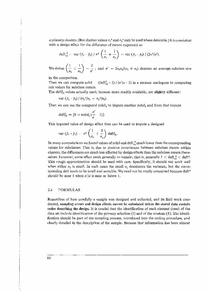
a primary clusters. (But distinct values a12 and a2

2 may be used where desirable.) It is consistent with a design effect for the difference of means expressed as

deft1; = var (.Yi - 512) / a2 (_!__ + _!__) = var Ch - ji2) J (2a2/11'). 111 112

(·1 1) 2 We define - + - = / ; and 11' = 2111112/(111 + 112) denotes an average subclass size

111 112 /1

in the comparison. Then we can compute rohd = (deft~2 - 1) / (n'/a - 1) in a manner analogous to computing roh values for subclass means. The defti2 values actually used, because more readily available, are slightly different:

var (.Y1 - .Y2) / (a1 2/111 + a2 2/112).

Then we can use the computed rohd0 to impute another rohd1 and from that impute

11' deft~2 = [1 + rohd1 (- - 1) ].

a

This imputed value of design effect then can be used to impute a designed

var (.Y1 - 512) = a 2 (_!__ + _!__) defti2. 111 112

In many computations we found values of rohd and deft1: much lower than the corresponding values for subclasses. That is, due to positive covariances between subclass means within clusters, the differences are much less affected by design effects than the subclass means them­selves. However, some effect tends generally to remain; that is, generally 1 < deft1: < deft 2. This rough approximation should be used with care. Specifically, it should not work well when either II; is small. In such cases the small II; dominates the variance, but the corre­sponding deft tends to be small and unstable. We need not be overly concerned because deft 2

should be near 1 when n' /a is near or below 1.

2.4 FORMULAS

Regardless of how carefully a sample was designed and collected, and its field work con­ducted, sampling errors and design effects cannot be cakulatecl unless the stored data contain codes describing the design. It is crucial that the identification of each element (case) of the data set include identification of the primary selection (i) and of the stratum ('1 ). The identi­fication should be part of the sampling process, introduced into the coding procedure, and clearly detailed in the description of the sample. Because that information has been almost

16

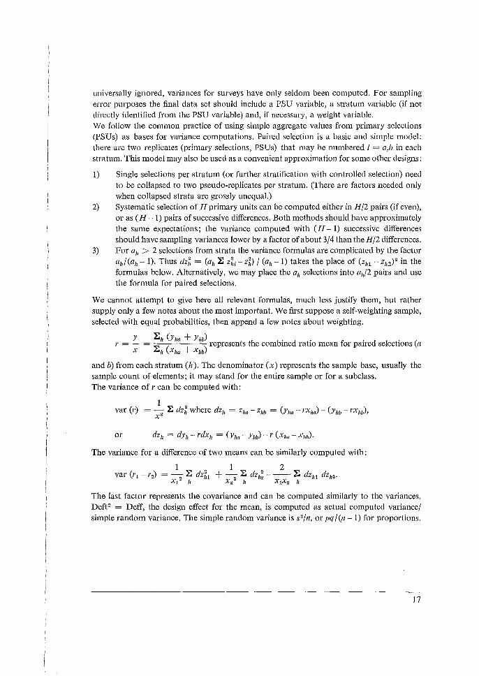
universally ignored, variances for surveys have only seldom been computed. For sampling error purposes the final data set should include a PSU variable, a stratum variable (if not directly identified from the PSU variable) and, if necessary, a weight variable. We follow the common practice of using simple aggregate values from primary selections (PSUs) as bases for variance computations. Paired selec(ion is a basic and simple model: there arc two replicates (primary selections, PSUs) that may be numbered i = a,b in each stratum. This model may also be used as a convenient approximation for some other designs:

1) Single selections per stratum (or further stratification with controlled selection) need to be collapsed to two pseudo-replicates per stratum. (There are factors needed only when collapsed strata are grossly unequal.)

2) Systematic selection of H primary units can be computed either in H/2 pairs (if even), or as (H -1) pairs of successive differences. Both methods should have approximately the same expectations; the variance computed with (H - 1) successive differences should have sampling variances lower by a factor of about 3/4 than the H/2 differences.

3) For a11 > 2 selections from strata the variance formulas are complicated by the factor a11 / (a1, - 1). Thus dz;, = (a 11 :E zl.; - zl.) / (a11 - 1) takes the place of (z111 - z112) 2 in the formulas below. Alternatively, we may place the a11 selections into a1,/2 pairs and use the formula for paired selections.

We cannot attempt to give here all relevant formulas, much less justify them, but rather supply only a few notes about the most important. We first suppose a self-weighting sample, selected with equal probabilities, then append a few notes about weighting.

Y :E,, (Y11a + Y11b) • • • • r = - = ..., ( ) represents the combmed rat10 mean for pa!fed selections (a

X "'11 X11a + X/Jb

and b) from each stratum ('1). The denominator (x) represents the sample base, usually the sample count of elements; it may stand for the entire sample or for a subclass. The variance of r can be computed with:

1 2 var (r) = - :E dz11 where dz11 = z1w - z11b = (Y1w - rx11a) - (y11b - rx,,b), xz

The variance for a difference of two means can be similarly computed with:

The last factor represents the covariance and can be computed similarly to the variances. Deft2 = Deff, the design effect for the mean, is computed as actual computed variance/ simple random variance. The simple random variance is s2/n, or pq / (n -1) for proportions.

17

We note that S 2 can be estimated by s 2 computed directly from samples of n elements, dis­regarding the complexities of the design, and the correlations between elements. An improved estimate of S 2 is s 2 [I + (deft 2

- l)/11] but this refinement is generally negligible because n is very large for the entire sample, and (deft 2 -1) should be small for subclasses [Kish, 1965, Section 2.8.C]. CV (x) = the coefficient of variation of x, the denominator and the sample base of the ratio mean r = y/x. For the entire sample x = n, the sample size; but it can be much less for subclasses, and for these CV (x) may be much larger. To avoid large biases and instabilities, CV (x) should be less than 0.2 and preferably under 0.1. We consider it essential to include the values of CV (x) in the computer print-out. In small subclasses of samples, some sample clusters may contain no elements, and X1za =

Yiw = 0 for these clusters. The methods proposed here, using combined ratio estimators, can yield useful estimates if the proportion of these empty clusters is not great.

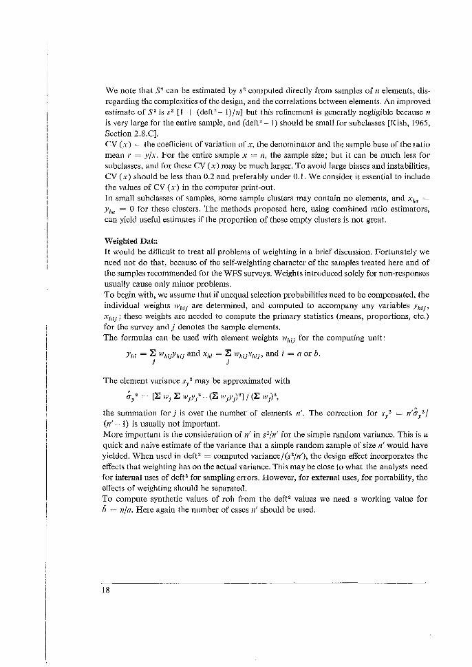
Weighted Data It would be difficult to treat all problems of weighting in a brief discussion. Fortunately we need not do that, because of the self-weighting character of the samples treated here and of the samples recommended for the WFS surveys. Weights introduced solely for non-responses usually cause only minor problems. To begin with, we assume that if unequal selection probabilities need to be compensated, the individual weights W1zu are determined, and computed to accompany any variables Y1zij, X1z;j; these weights are needed to compute the primary statistics (means, proportions, etc.) for the survey and j denotes the sample elements. The formulas can be used with element weights W1zu for the computing unit:

Y1zi = :E W1zuY1zij and x,,i =I: w11 ijx1zu, and i =a orb. j j

The element variance s/ may be approximated with

0-Y 2 = [!: wj I: wjy/- (:E wjy)2] I (:E w)2,

the summation for j is over the number of elements n'. The correction for s/ = n' a// (n' - 1) is usually not important. More important is the consideration of n' in s"/11' for the simple random variance. This is a quick and naive estimate of the variance that a simple random sample of size n' would have yielded. When used in deft 2 = computed variance/(s2/n'), the design effect incorporates the effects that weighting has on the actual variance. This may be close to what the analysts need for internal uses of deft 2 for sampling errors. However, for external uses, for portability, the effects of weighting should be separated. To compute synthetic values of roh from the deft 2 values we need a working value for b = n/a. Here again the number of cases n' should be used.

18

The factor (1 - f) for finite population correction has been neglected above, because it is usually negligible, as it will be for the WFS samples. The simple variance formulas above are based on simple aggregate computing units for primary clusters. To compute separate components for successive stages of selection becomes much more complicated. For multipurpose samples, we believe, it is better strategy to provide basic and reliable techniques that can be used simply for many variables.

2.5 VARIABILITY OF COMPUTED SAMPLING ERRORS AND THE NEED FOR AVERAGING

Sampling errors computed from survey samples are themselves usually subject to great sampling variability, and so are estimates of deft and of rob derived from them. Sampling theory, and experience with many and repeated computations, teach us not to rely on the precision of individual results, even when these are based on samples with large numbers of elements. The variance of computed estimates of sampling errors is a function primarily of the number of primary units used in the computations. For example, if 2L PSUs are used as paired selections from L strata, the computations of standard errors are subject to coefficients of variation greater than 1 / \/(2LY. Thus for samples confined to 50 or 100 PSUs in 25 or 50 strata, the coefficients of variation of computed standard errors are 14 or 10 per cent. Hence the computed values of deft are also subject to coefficients of variation somewhat over 14 or 10 per cent for samples of 50 or 100 PSUs. This implies, for example, that a value of deft = 2.0 is subject to standard errors of 0.3 or 0.2. Such precision, though not useless, is not sufficient to distinguish design effects for individual variables. The coefficients of variation of variances, hence of deft2, are roughly . ..j(2/L), twice as great as for standard errors. For values of deft 2 near 1, the computed values of deft 2-l, hence of roh, are subject to wild variation. These give rise often to negative values of roh that are spurious. However, for design purposes the higher values of roh and deft usually have greater importance than the lower values. Few samples are based on large enough numbers of PSUs to yield sufficient precision for individual estimates of sampiing errors. Such samples can be of three types:

1) Samples of elements selected directly and independently (or stratified) from a list, with variances so computed.

2) Large samples of a city or county where several hundred small clusters are selected directly.

3) Large national samples with several hundred PSUs, such as the national labor force surveys of the U.S.A. and of Canada.

* For this reason simple replication methods are not much used in practical survey work. For 4 or 10 replications, hence 3 or 9 'degrees of freedom,' the coefficient of variation of sampling errors is of the order of . ..j(l/6) = 0.4 or . ..j(l/18) = 0.25

19

4) Periodic surveys which can take advantage of replication of similar sample designs and statistics by averaging sampling errors, and values of <lefts and rahs derived from them, computed over several periods for similar statistics.

However, most surveys are not periodic, nor based on hundreds of PSUs. Computations of sampling errors, of clefts, and rahs derived from them, are subject to great variability. In addition, most surveys are highly multipurpose in nature and we must combine results from diverse statistics for joint decisions and designs. For both of these reasons we need to combine somehow the results of computations over many statistics. This implies, primarily, combining results for different variables and, secondarily, for diverse subclasses of single variables. Averaging over similar variables from periodic surveys, or for categodes of one variable (e.g., age classes), seems reasonable. However, technical and analytic justifications appear more difficult for combining and for averaging results over different variables in a single survey. Sampling errors for diverse variables are indeed very distinct, and many of these distinctions we can now understand and recognize. Each of our surveys shows about a hundredfold range in rahs computed for about 40 variables. We found that roh values of 0.001 to 0.005 are common for basic variables like age, whereas 0.1 is often found and some­times even 0.2 for some socio-economic and attitudinal variables. Such variation would be reflected in similar increases in the values of (deft 2-l). It merely appears to be reduced in the values of deft 2, and the variation appears further reduced in the values of deft actually printed in our tables. But those variations are real and important both for inference and for planning other designs. The diversity among sampling errors is further compounded by the necessity to look beyond the means of variables based on the entire sample. Just as important in many surveys are means based on subclasses, and comparisons between those means. (We shall not pursue here even deeper difficulties for more complex measures of multivariate relationships.) These should also be considered, though they are commonly neglected. However, the double and triple complexity of variables (characteristics) x subclasses x comparisons is not only difficult to compute, it is even more complicated to present clearly, and very difficult to comprehend usefully. Despite the recognized differences between variables, combining their results is preferable to its alternatives. We should not follow the common practice of choosing a single variable among many for making inferences about the design and for further designs. Nor would it be practical to try to build separate designs based on the extremely diverse results for many survey variables. These complexities drove us to find some ways to relate results for the entire sample to results for subclasses, and these to the results for their comparisons. Some relationships that are reasonably useful were found. Though subject to variations, these appear small compared to the large variations we find generally for diverse variables. These relationships are discussed in the next two sections.

20

2.6 STRATEGIES FOR SAMPLING ERROR COMPUTATION

We assume that the computations of sampling errors should be primarily useful to four kinds of people:

1) demographers directly engaged in primary analysis and presentation of the results; 2) social scientists who use the data later for secondary analysis; 3) the larger public who reads the work of the first two types; and 4) sampling statisticians attempting to design other studies in similar survey conditions.

The primary analysts and probably the secondary also, should have access also to detailed results of the computations. The needs of the larger public are best served with some simple tables of sampling errors, incorporating averages of design effects and rahs. Other sampling statisticians can utilize both detailed and summary tables. The sampling statisticians who compute the sampling errors should have all kinds of users in mind. The choice of variables and categories for subclasses should be performed in collab­oration with the primary analysts of the data. To meet the needs of the various users, several guidelines for the sampling statisticians are proposed. First and most important: compute sampling errors for many variables of many kinds. We found very wide ranges in values of sampling errors (stands.rd errors and design effects) between diverse variables within the same surveys. Hence we think it inadequate to single out arbitrarily one or a few as the critical survey variables for sampling error computations. Nor is it much better to do so for several categories (e.g., classes of age or of occupation) of only one or two variables; differences between categories tend to be much less than between variables. The range of variables should parallel the important aims of the survey, of its analysts and of its users. It should also deliberately aim to cover the range of design effects for diverse kinds of variables. Separate the variables into a few groups within which the sampling errors, the defts and rohs, are relatively similar. Creation of groups that are meaningful and useful is a difficult and uncertain task. Our attempts in the five country reports remain tentative. It is crucial that sampling errors be provided not only for the entire sample base, but also for a wide range of subclass means, aml fur comparisons (differences) between subclass means. We can distinguish several kinds of subclasses:

1) Major divisions of the entire sample into two or a few parts may be subject to drasti­cally different sampling procedures. For example, suppose that in cities the primary selection units are elements or very small clusters, whereas in rural districts large primary clusters (e.g., villages) are selected. Sampling errors and def ts, needed separately for cities and rural places as sample bases, can be very different, and perhaps computed

21

and presented separately. (However, combined overall results may also be needed, as for the Malaysian data.)

2) Segregated classes in separate strata, such as regions of the population, also used as bases of separate analysis of results, may be subject to different sampling procedures, different size clusters (b), or possess different homogeneity (roh). In those cases separate computations may be needed, and justified if the sample bases in primary units (a) are large enough to yield reasonably stable results. Usually, however, separate regions have only few primary units, and are subject to similar selection procedures. Differences in design effects, though present, are often relatively minor. They may be difficult to detect without extensive computations that may not be worthwhile. The best strategy may be to infer the same design effects as for the entire sample, subject only to major and relevant differences in composition, such as city/rural proportions, as noted in (1).

3) Cross-classes are typically the most numerous and important subclasses in the popula­tion: subclasses that cut across the major aspects - clustering and stratification - of the sample design. Age, sex, social status, income, education, most occupations, attitudinal subclasses, tend to be cross-classes, more or less. Design effects tend to decrease linearly almost to 1, as cross-class sizes decrease, and rohs remain relatively constant.

4) Mixtures between cross-classes and segregated classes are less common than either extreme, we believe, but they do occur. Ethnic groups and some localized occupations (farmers, fisherman, miners, woodsmen) may present problems for special attention.

Computing sampling enors for a wide range of variables based on the entire sample may be sufficient if design effects seem uniformly small because cluster sizes (11/a) were small. For two samples of cities (Ankara and Mexico City) this appeared to be the situation. Uniformly small values of roh would also result in small deft 2 values, but we have never encountered that situation. For small values of deft" on the entire sample, the values for cross-classes may be guessed well enough. For example, for a sample of many clusters of 4 to 6 elements, deft1

2 values for the total sample may be mostly in the neighbourhood of 1.1, with most or all under 1.2 or 1.3. One may guess confidently that for cross-classes of proportion M,, the deft; values are bound to be rather close to [l + (deftr -1) M.]. (This simple approximation balances over­estimation by roh (1 - M.) with underestimation because rohs tends to be larger than rohr .) Thus for subclasses of Ms = 0.2 of the sample, defts 2 are guessed to be near 1.02 or 1.04, and better estimates may not be worth computing. For larger values of deft? it is probably worthwhile to compute sampling errors for cross­classes. This is desirable because the survey data should be supported with their own error computations; also because these could be useful additions to our sparse knowledge. How­ever, if funds or human resources are not adequate for cross-class computations, our present

22

results provide reasonably sound and reliable grounds for imputing from rohs computed for the entire sample to rohs, and then to design effects, for subclass means and for their differ­ences. When sampling errors are computed for subclasses, several choices must be made with regard to the kinds and numbers of variables chosen. We can give some advice, although situations differ, and this subject is due for evolutionary development. In this discussion we denote by characteristics the variable of primary interest, to distinguish them from the subclass control variables. Characteristics appear in the numerator, and subclasses in the denominators of means and proportions. For differences of pairs of means we generally use the same characteristic in the numerator, and two different categories of the same subclass variable in the denominator. For example, births to 20-24 year-olds versus births to 25-29 year-olds. Now for some guidelines to a strategy for computing sampling errors.

1) Compute sampling errors based on the entire sample for many characteristics. Then go on to subclasses and comparisons, unless that seems unnecessary or unfeasible, as discussed above.

2) Compute sampling errors for many characteristics, perhaps for all those in 1), based on a moderate number of subclasses. Sampling errors, particularly rohs, were found subject to greater diversity across characteristics than across subclasses.

3) Analysis of all (or most) chosen characteristics by all chosen subclasses (rather than using different subclasses for each characteristic) leads to easier handling. This yields a symmetrical table of characteristics by subclasses. However, other designs may be used, especially for a larger number of subclasses.

4) Use more variables, each for one or a few categories, rather than exhausting all categories for a few variables. Variability between variables is generally greater than between categories within variables. This is especially true for characteristics, but also for subclass variables.

5) We recommend a standard procedure for computing sampling errors for the means of two subclasses of one variable jointly with the difference of the two means. For many subclass variables one or two pairs usually suffice. Members of each pair should usually be mutually exclusive (non-overlapping) but not usually exhaustive.

6) In choosing subclass categories use a range of subclass sizes to obtain empirical evidence by sizes of subclasses for investigations of deft 2 and of roh. Combine the coded cate­gories to suit your aims.

7) Most of the needed subclasses tend to be (approximate) cross-classes. However, partially segregated subclasses (ethnic, socio-economic, etc.), if important, should be investigated also.

23

3. Summary of Results from Eight Surveys

3.1 INTRODUCTION (TABLE 1)

The tables and discussions that follow report on calculations of sampling errors - standard enors, design effects and rohs as dealt with in the previous chapter - for 8 fertility surveys from 5 countries: South Korea, Taiwan, Peru, Malaysia and the United States. Sampling errors were computed for about 30 to 40 characteristics in each case. This was done in each survey for means based on the entire sample and on about 24 subclasses, and for differences between about 12 pairs of subclass means. We used mostly symmetric designs for the analysis: each of a set of characteristics based on each of a set of subclasses. Thus for each survey over 30 x 24 = 720 sampling errors were computed for subclass means, plus over 30 x 12 = 360 for differences between pairs of means. In each case averages for each of the 30 charac­teristics over the 24 subclasses and over the 12 comparisons were computed; also averages over the 30 characteristics for each of the 24 subclasses and 12 differences. Much of the discussion in this summary and in the 5 separate reports concerns the relationships of sampling errors for entire samples to those for the averages (or 'marginals') over subclasses. The great range in values of roh for different variables in each of the surveys is the most important result in all these data. The roh values have an effective hundredfold range in each survey from about 0.001 to 0.002 or about 0.1 or 0.2. Values as low as 0.001 or 0.002 appear and can cause, with sample clusters of 50 or 100 elements, a 10 per cent increase in variance. Lower values of roh can be considered negligible; and many of them, especially negative rohs, are due to the sampling variability of the computations. There are a few roh values higher than 0.2, but these can be considered individually. The great range of roh values implies a similar range for values of (deft2-1) based on the entire sample, though for the deft values shown, the numerical range is less. The great ranges we found lead us to our strategies of computation and of presentation. We believe it is essential to compute for each multipurpose survey the sampling errors for a large number of important variables, rather than only for one or a few 'critical' or 'typical' variables. The presentation should make some allowance for different types of variables, with some flexibility for the judgment of the reader. Some differences between types of variables can be detected on each survey. However, these differences are not consistent, and are also masked by considerable sampling variability. Hence, instead of sorting the variables into separate tables, we distinguish them with a code of 1 to 6 shown in the tables, where all variables (characteristics) appear arranged in de­creasing values of rohs. Deft values follow these decreases closely, except for minor differ­ences, due to slight differences in sample bases (n), hence cluster sizes (11/a). Here the reader can pick out the placing of each of the 6 types of variables, by using their codes in the very

24

first column on the left. The reader can adjust the codes and the typing to suit his needs and ideas. Socio-economic variables (5) appear noticeably high on the lists for Korea and Peru. Demo­graphic Background Variables (6, age, marriage) tend to be near the lower end for all surveys. Attitudes (4) and Birth Preferences (3) appear remarkably high in Taiwan, but not elsewhere. Contraceptive Practice (2) appeais widely spread, though more often in the lower half. The most important type, Fertility Behavior (1), appears mostly in the lower half, with roh values mostly from 0.005 to 0.05; for purposes of design, using 0.02 or 0.03 will not mislead one badly. Inconsistencies for types within surveys seem due mostly to random variations in computed sampling errors and to haphazard factors in the choices of variables. Inconsistencies between surveys have additional sources as well: different kinds of sampling units and different sizes of sample clusters in various stages; the distribution of variables in the population; and the contribution of interviewer variance to the response error. Hopefully these factors will be investigated in the future. Yet the ranges of variation within types seem considerably less than the range of 50 or 100 for rohs of all variables within surveys, more like a factor of 5 or 10. Especially fertility behavior (1) seems to range mostly from 0.005 to 0.05, as we noted above; it also seems fairly consistent across surveys. Thus the typing of variables seems an effective and simple way to reduce the range of our ignorance by a factor of about 10. Above we considered the sampling errors of characteristics over the entire samples. These are the most basic statistics. They are also the sources of the greatest range of diversity. This diversity is closely reflected in the averages for each of the same characteristics over subclasses. These averages of rohs show close relationships to the basic overall rohs: the ratios of the former to the latter run relatively close to a mean value of about 1.2. Second only to the above considerations in importance are the consequences of different sizes of subclass bases used commonly in analysis. From surveys of several thousand cases, some important means may be based on only a few (or one) hundred cases; thus the range of variation of subclass bases may be 10- or 20-fold. Using deft values unadjusted from the entire sample would (and often does) result in gross overestimation of sampling errors for most means based on subclasses. To generalize among subclasses, we must remove the unwanted effects of the size of the subclass base. To remove those effects we computed synthetic rohs and analyzed them. The individual computations of rohs for each characteristic/subclass combination (about 30 x 24 for each survey) are subject to great variability; but the average roh for each char­acteristic computed over several (about 24) subclasses is quite stable. The ratios of these averages to the corresponding rohs for the overall means are generally rather close to the mean values of these ratios. We refer to subclasses that are approximately cross-classes, more or less evenly distributed in the sample clusters; other kinds of subclasses, those that are very unevenly distributed in sample clusters, need special consideration.

25

We then computed the ratios of the means of subclass rohs to the rahs for the entire sample We computed these ratios for many variables on each survey to observe this relationship Fair stability was found, except for very small rahs (below 0.010, say) where it means and matters less. The average over all variables of these ratios is mostly between 1.15 and 1.40 for the different surveys. Furthermore, we note that the ratios tend to be less for demographic subclasses than for socio-economic subclasses: say 1.2 versus 1.4. We expected some difference because the former are closer to being cross-classes than the latter; this is shown by considerable (several­fold) differences of rahs on each survey when the subclasses are viewed as characteristics over the entire sample. These large differences between types of subclasses have relatively small effects on the ratios of subclass rahs to total rohs. This stability is reassuring for our proce­dures of imputation, since the behaviour of subclass rohs is becoming understandable. There remain variations and uncertainties, but these are minor when compared to the ten- and hundredfold ranges we have dealt with earlier. Finally, we also compute synthetic values of rohd for differences between pairs of subclass means. These incorporate artificially the effects of positive correlations (covariances) between the compared subclass means. The rohd values are reduced thereby, and the ratios of these rohd values to respective mean subclass rahs average mostly between 0.1 and 0.5. Using 0.3 as a rough starting point, one will not be too far wrong in ones estimate of the corresponding deft values. Here we note more looseness than above. We hope that future work, both theoretical and empirical, may yield tighter limits. These values are subject to more sources of variation, both random and structural. The degree of variation is less than the customary assumptions of either no design effect or of no covariance, which amount to adopting ratios of rohd to subclass rahs of 0 or 1.0. Also, relating rohd to corresponding mean subclass rahs takes us again well below the ten- or hundredfold variation with which we began. For clusters of b = lOOandroh = 0.5the design effect would bedeftf = [1 + .05 (100-1)] = 6 for the entire sample. However for cross-classes of about 20 per cent (such as a 5-year age group from all women 15-40) the effective cluster is only b = 20, and the design effect only deft; = [1 + 1.2 (.05) (20 - 1)] = 2.2. For the difference of two cross-classes, if we impute a factor of 0.2, the defta = [1 + 1.2 (0.2) (.05) (20 - I)] = 1.2. Thus whether the overall means, or subclass means, or their differences (or other analytical statistics) are most im­portant becomes a crucial decision of design. Subclass clusters averaging 20 interviews may not be far from optimal cluster size for some reasonable cost factors; for example, birth rates by 5-year age groups of women involve cross-classes approximately of. 20 per cent. However, note that these age-specific birth rates combined into an overall birth rate will tend to have the overall deft 2 of about 6, and suffer from too large clusters of 100. Table 1 summarizes a vast body of computations over a diverse set of eight surveys in five countries. Since the variables included had not been co-ordinated initially, it is comforting that some very useful stabilities may, nevertheless, be drawn from them. But, first, we wish

26

i I

to exclude from our remarks some data, marked with an asterisk (''), that we included for completeness. The black sample of 1970 from the United States has uniformly high roh values out of line with all others; we put no confidence in the sample design for drawing inferences to other samples, as we noted in the analysis. The sample from Malaysia includes some ethnic and geographic subclasses that are so far from being cross-classes that they should not be included with the others. In the 1970 white sample from the U.S. the roh value of 0.105 for age at marriage is way out of line for other similar variables here and elsewhere, for reasons unknown. The average values of overall robs (row 0) varies from 0.024 to 0.063. This stability is quite good, considering the diversity of variables included and of the sample designs used in the eight samples. It is helpful for choice of sample designs, since accepting 0.04 or 0.05 for roh would not mislead one. For the most important variables, fertility experience (row and code 1), the roh values are lower and more stable, 0.011 to 0.034. One may use 0.02 for a rough average. The demographic background variables (age, marriage: row and code 6) are similar. For general attitudinal variables the roh values are very high for Taiwan and Peru, and fertility preferences are also high in Taiwan. It would be interesting to investigate how much of these high rob values is due to homogeneity of the respondents in compact clusters, and how much to the effects of 'interviewer variance' of responses from large work-loads. The high roh values for socio-economic variables in Peru and South Korea have implications for sample designs, as well as for sociological studies of their sources. For subclasses (Part B), the ave'rage rohs tend to reflect the rohs for the total sample. Thus the ratios of subclass to total rohs are relatively stable from 1.15 to 1.41 (row 9). This ratio in Malaysia is higher because the half of the 20 subclasses are segregated, as we noted above; the 10 cross-classes among them average 1.15. The value of 2.00 for the 1960 U.S. white sample is based on only 8 subclasses, and removing one of them reduces the ratio to 1.15. 'Nhen we separate socio-economic subclasses from others (age, and other demographic background), we note, regularly, considerable differences between the two groups, when these are computed as characteristics based on the entire sample; the ratios of the rohs of row 12 to row 13 are several (6 to 20) fold. However, when used as subclasses (rows 14 and 15) the differences between the two sets of subclass rohs are not great, perhaps a ratio of 4 to 3. This is comforting: we need not be too worried about subclasses that are not 'true cross­classes'. However, we should remain cautious about segregated classes like geographical domains, as the data in Malaysia show. For these subclasses deft 2 rather than roh may tend to remain constant. The ratio of the synthetic rohs for differences to the average rohs for subclass means (rows 10 and 11) is less stable in relative terms. To get beyond random and haphazard sources of variations to causes and models is beyond our present resources. In all cases the reductions, due to covariances between clusters, are substantial. The central value may be 0.1 to 0.2.

27

TABLE 1

Summary of Average Robs for 8 Surveys

2 3 4 5 Sa 6 7 8*

So. Korea Taiwan Peru Malaysia United States '71 '73 All Xe lass '60W '70W '70B

A. ROHS FOR TYPES OF VARIABLES FOR TOTAL SAMPLE (AND NUMBERS OF VARIABLES)

0. All characteristics .050 .033 .059 .063 .045 .024 .037 .136* 40 39 40 29 29 9 36 36

1. Fertility Experience .016 .009 .014 .034 .025 .011 .019 .098* 11 6 9 8 3 4 5 5

2. Contraceptive Practice .047 .021 .030 .054 .022 .043 .029 .137* 9 11 9 8 3 2 8 8

3. Fertility Preferences .023 .024 .072 .028 .025 .019 .142* 6 8 11 0 3 2 6 6

4. Attitudes .028 .026 .145 .094 .017 .051 .150* 2 3 8 1 2 0 16 16

5. Socio-economic Variables .128 .081 .016 .126 .045 9 8 2 7 12 0 0 0

6. DemographicBackground .014 .025 .025 .024 .olO .039 .105* .092* 3 3 1 5 2 1 1 1

B. ROHS FOR SUBCLASSES AND FOR DIFFERENCES

Number of Variables 40 39 40 20 14 14 9 36 36

Number of Subclasses 23 22 24 10 20 10 8 24 24

7. Rohs for Total Sample .050 .033 .059 .056 .028 .028 .024 .037 .136*

8. Rohs for Subclasses .059 .044 .079 .065 .055* .032 .048 .052 .157*

9. Ratio of Subclass/Total 1.19 1.36 1.33 1.15 2.00* 1.15 2.00 1.41 1.15

10. Differences of Means .0060 .0000 .0065 .017 .036* .007 .013 .005 .007

11. Ratio ofDiffer./Subclass .100 .000 .083 .026 .64* .21 .27 .096 .045

C. COMPARISONS OF SUBCLASSES: SOCIO-ECONOMIC (SE) VERSUS CROSS-CLASSES

12. SE as Variables .076 .092 .042 .105 .210* .122

13. Other Variables .006 .007 .002 .015 .037 .020

14. SE Subclass Base .063 .040 .088 .073 .075* .063

15. Other Subclass Base .057 .038 .069 .063 .032 .047

* These data are included for completeness only; see page 27.

28

3.2 SOUTH KOREA FERTILITY SURVEYS (1971 AND 1973) (TABLES 2-7)

3.2.1. SAMPLE DESIGNS

The 1971 National South Korea Fertility/Abortion Survey sample was drawn from the enumeration districts, of roughly equal sizes, for the 1970 Census. The 75,150 ordinary districts (2067 special districts, covering such special populations as military institutions, were excluded) were stratified into the categories, Seoul, Other Urban, and Rural. The districts within each of these broad categories were ranked by size of population and divided into further strata with equal number of districts per stratum. This yielded thirty-one strata of approximately equal numbers of units: 8 in Seoul (1827 districts per stratum), 10 in Other Urban (1787 districts per stratum) and 13 in Rural (1641 pairs of districts per stratum). The sampling units were defined as one enumeration district in Seoul and Other Urban strata and as a pair of contiguous districts in the Rural stratum. Two sampling units were selected from each stratum with probabilities 1/910 in Seoul, 1/890 in Other Urban and 1/820 in Rural. These fractions were deemed sufficiently constant to justify omitting weights to compensate for unequal probabilities of selection. The final sample was of size 6,284 households spread over 62 units: (88 enumeration districts) from 31 strata. All ever-married women in all sample households were defined as respondents for the survey.* The 1973 South Korea Fertility and KAP Survey is also based on a stratified one-stage cluster sample drawn from 1970 Population Census enumeration districts. The total number of areas was first divided into rural and urban strata. Within each stratum, areas were arranged by geographical location and occupation. Using equal-probability systematic selection, 42 enumeration districts were selected: 19 in the Urban stratum and 23 in the Rural stratum. The sample size was 1919 respondents. For sampling error computations a paired selection design was imposed that reflected the order of systematic selection. To obtain even numbers of units in both urban and rural strata, the largest units in each were split in two. The 44 computing units were then paired (1, 2), (3, 4) in 22 computing strata. An effort was made to define statistics from both the 1971 and 1973 surveys to increase the overlap of variables. However, the effort was only partly successful (see Table 4), because of differences between the two surveys' target populations, questions asked and coding.

3.2.2. RESULTS FOR THE TWO TOTAL SAMPLES

Tables 2 and 3 (Columns 1-4) present the means, standard errors, design effects (defts), and intraclass correlations (roh) for the 1971 and 1973 surveys. Results have been listed in order of decreasing roh. In the 1971 survey the mean deft and roh are respectively 2.155 and .050. These results differ markedly from the corresponding 1973 survey results of 1.471 and 0.033. Larger cluster sizes in the 1971 survey tend to induce the larger deft 2 = 4.64, versus deft 2 = 2.16 in 1973; the 1971 survey has n = 6284 from 62 units giving an average cluster size of 101, whereas the

* For further details on sample design see: Moon, M. S., Han, S. M., and Choi, S., Fertility and Family Planning, Korean Institute for Family Planning, Seoul, Feb. 1973, pp. 9-13.

29

1973 survey has 11 = 1919 from 44 units giving an average cluster size of only 44. Rohs generally vary from 0 to 0.2 in 1971 (Table 2) and from 0 to 0.1 in 1973 (Table 3). An attempt is made in Table 4 to draw a more controlled comparison between the two surveys by considering only those variables that are common to the two. Results are ordered by decreasing value of the 1973 roh. Now the average <lefts and robs from 1971 are respectively 1.963 and 0.037 while the corre!;ponding figures for 1973 arc 1.421 and 0.030. It seems that choice of variables produced much of the difference in average roh values between Tables 2 and 3. However a sizeable difference between deft 2 values remains, 3.85 versus 2.02, as expected from the designs. However, the roh values are rather consistent for items for the two years. In the last column, 9 of the 23 relative differences are negative; most of the variation appears haphazard. Only for variables 510 and 232 are the differences remarkable and important. For 232 we may suggest a possible cause: more even distribution of visits by health workers in 1973 than in 1971. However, the difference for 510 puzzles us and makes us wonder about differential interviewer effects in the two studies.

3.2.3. AVERAGE RESULTS FOR SlX TYPES OF VARIABLES

A summary of the results of Tables 2 and 3 is presented in Table 5 for the various categories of variables. Comparisons of types are probably more reliable than those between the two surveys due to differences in variables chosen. In both surveys it is evident that socio-economic variables have the highest rahs. Fertility experiences, probably the most important type here, have the lowest rohs. Demographic variables also have low rahs. These 1esults are consistent with those from the other surveys. Attitudes and preferences also have rather low average rohs. The decrease in roh from 0.047 to 0.021 for contraception practices may in fact denote a diffusion of birth control from 1971 to 1973.

3.2.4. RESULTS FOR SUBCLASS MEANS AND COMPARISONS

The subclass rahs in column 5 of Tables 2 and 3 are averages for all variables over the 24 subclasses for which computations were made. We excluded one variable from the 1973

tabulations, and one subclass from the 1971 tabulations, due to mistakes we made in their coding. A few exclusions were made for those subclasses that indicated, with large values of CV (x), extreme instabilities. These were due mostly to 'empty' PSUs; agricultural labourers serves as a good example, and the smaller 1973 sample had more of this trouble. The values in column 5 decrease along with the ordering of column 4, generally, but not evenly. The ratios in column 6 of subclass to overall rahs (column 5/column 4) vary around averages above unity. The variations are greater for the 1973 sample, because it is smaller in numbers of both respondents and units. Also in both columns the variations near the bottom are great, being ratios of two small and unstable numbers. The averages of the ratios of subclass to total roh (see column 6) in the 1971 and 1973 surveys are respectively 1.50 and 1.15. (In calculating the 1973 average the entries for 236 and 139 were omitted due to their exceptional

30

fl.,

size). Another such indicator may be calculated by taking the ratio of the mean of the mean rohs over subclasses (columns 1 and 5) to the mean of the rohs for the total sample (Tables 2 and 3). For the 1971 and 1973 surveys these figures me respectively 0.0589/0.0496 :::: 1.19 and 0.0444/0.0327 :::: 1.36. These ratios of means seem better than the means of ratios given above, because they give greater weight to the larger rohs, which are more important. Subdass tesults are further analyzed in Tables 6 and 7. In columns 1 3 results are given for the proportion of the total sample belonging to a given subclass category, and deft and roh for the subclass categories treated as variables. These reflect the degree of clustering for the subclasses. In columns 4 and 6 are given, respectively, the mean rohs over almost 40 variables for each subclass and the mean rohs for differences of subclasses. In both surveys, looking at column 3, it is clear that the socio-economic subclasses, taken as proportions of the total sample, exhibit considerably higher roh than do the demographic variables, as expected. In the 1971 survey, the average rohs for the 11 socio-economic variables was 0.076 and 0.0065 for 12 demographic variables. In the 1973 survey, the corresponding figures were 0.092 and 0.007. It is interesting to note that for the demographic variables, which were defined the same way in both surveys (except for age categories), the mean rohs are similar. Individual discrepancies may be found, but few large enough to justify particular attention. The socio-economic variables are different in the two surveys mainly due to the fact that religion was not covered in the 1973 survey. However the overall roh is still fairly constant over the two surveys. If we look at the results averaged over variables within subclasses (columns 4-6) we note a remarkable stability in average rohs in the 1971 survey and a little more variation in the 1973 survey. This difference between the surveys results from the smaller sample size in the 1973 survey. Note, too, that in both cases the avernge robs from the socio-economic subclasses are only slightly larger than the average rob for the demographic subclasses: variation in robs is primarily due to substantive variables and not to subclasses. These relations of subclass robs are consistent not only between these two samples, but also with similar computations from the samples from other countries. Thus when defining variables for sampling error purposes, it is advisable to aim for a wide variety of variables over fewer subclasses. All of the results presented here fall well within the reliability criterion of the coefficient of variation of sample size CV (x) being less than 0.2. For the large sample size of the 1971 survey this presents no problem with the coefficient of variation ranging around 0.025 for totals and rising to a maximum of 0.087 for subclasses defined in this set of runs. In the 1973 survey, however, CV (x) was larger with values around 0.04 for the total sample, and for a few subclasses it exceeded 0.2. These results in Table 7 have been omitted and starred. Synthetic roh (or 'rohd') values for differences between pairs of subclass means are presented in column 6 of Tables 6 and 7. These values are also averages over the almost 40 variables. Nevertheless, they are highly variable, (the 40 individual values much more so). For the 1971 survey the ratio of the rohs for differences to subclass means is 0.148, 0.04-6, and 0.100, respectively, for the 11 socio-economic, 12 demographic, and the 23 combined subclasses.

31

TABLE 2

South Korea Fertility Survey [1971]

Sampling Errors for 40 Variables

2 3 4 5 6

Variable* Variable Description Mean Std. Deft Roh Mean Ratio Number Error Subcl. 5/4

Roh

516 No. Modern Objects 3.47 .163 6.052 .355 .401 1.13 515 Intend High School for Daughters 0.62 .028 3.943 .191 .152 0.79 232 No. Health Worker Visits 0.50 .081 4.486 .191 .212 1.11 513 Sales, Clerk, Prof., Husband Occ. 0.37 .027 3.977 .182 .185 1.02 514 Intend High School for Sons 0.83 .019 3.513 .139 .092 0.66 509 Buddhist or Confucian 0.22 .016 3.144 .089 .099 1.11 530 Religion None/Unspecified 0.65 .017 2.762 .066 .075 1.14 512 School 10 + Years, Husband 0.29 .015 2.554 .055 .054 0.99 434 Children Should Support Parents 0.70 .014 2.478 .051 .089 1.74 237 Ever Used Abortion 0.24 .013 2.419 .048 .053 1.10 511 Reads Papers Daily 0.14 .010 2.364 .046 .064 1.40 228 May Use Abortion 0.54 .015 2.361 .046 .034 0.76 231 No. Health Center Visits 0.28 .027 2.177 .037 .039 1.04 207 No. Induced Abortions 0.53 .035 2.162 .037 .048 1.32 321 Ideal No. of Children 3.25 .041 1.961 .034 .068 2.01 333 Thinks Male Heir Needed 0.57 .013 2.018 .031 .042 1.38 105 No. of Live Births 4.17 .064 2.012 .030 .034 1.13 104 No. of Living Children 3.54 .049 1.925 .027 .028 1.04 510 School 10 + Years, Wife 0.10 .007 1.887 .026 .049 1.91 320 No. of Ideal Sons 1.97 .022 1.729 .024 .054 2.28 224 Ever Used Pill 0.19 .009 1.827 .023 .031 1.33 136 First Birth Interval (mos.) 26.14 .398 1.812 .023 .019 0.83 602 Yrs. Marriage Duration 14.74 .223 1.783 .022 .034 1.56 635 Married Age 18-24 0.95 .005 1.705 .019 .026 1.36 225 Birth Control Ever Used 0.36 .010 1.700 .019 .029 1.44 139 No. of Living Sons 1.85 .029 1.688 ,018 .012 0.67 318 No. of Additional Children Wanted 0.66 .023 1.591 .018 .052 2.87 140 Ever Have Miscarriage 0.31 .010 1.634 .017 .021 1.24 319 No. of Total Children Wanted 3.50 .040 1.554 .017 .045 2.72 138 Mos. Open Birth Interval 46.45 .802 1.614 .016 .036 2.23 108 No. of Total Pregnancies 5.08 .060 1.608 .016 .034 2.15 106 No. of Miscarriages 0.25 .012 1.582 .015 .014 0.95 317 No. of Additional Sons Wanted 0.46 .015 1.463 .014 .047 3.45 227 Using Birth Control 0.19 .007 1.497 .012 .018 1.45 126 No. of Pregnancies Before Contr. 3.48 .059 1.200 .010 .025 2.54 223 Ever Used Loop 0.19 .007 1.310 .007 .007 1.00 122 Fecund 0.62 .008 1.288 .007 .016 2.36 429 Think Abortion OK 0.41 .008 1.223 .005 .013 2.53 601 Currently Married 0.90 .004 1.129 .003 .004 1.38 103 Currently Pregnant 0.10 .004 1.081 .002 .002 0.96

Mean Over 40 Variables 2.155 .0496 .0589 1.50 Ratio of Means Col. 5/Col. 4 1.188

* The first digit of the Variable Number denotes: 1) Fertility Experience, 2) Contraceptive Practice, 3) Birth Preferences and Desires, 4) Attitudes, 5) Socio-economic Background, 6) Demographic Variables.

32

TABLE 3

South Korea Fertility Survey [19731

Sampling Errors for 39 Variables

2 3 4 5 6

Variable* Variable Description Mean Std. Deft Roh Mean Ratio Number Error Subcl. 5/4

Roh

513 Sales, Clerk, Prof., Husband Occ. 0.40 .030 2.674 .146 .145 1.00 512 School 10 +Yrs., Husband 0.41 .025 2.203 .091 .070 0.77 509 Urban Background 0.27 .022 2.204 .091 .122 1.34 530 Rural Background 0.63 .024 2.155 .086 .110 1.28 510 School H. S. +,Wife 0.18 .018 2.119 .082 .089 1.08 511 Wife Currently Working 0.09 .013 1.939 .066 .107 1.63 232 Family Planning Worker Contact 0.25 .019 1.898 .062 .131 2.11 315 Can Plan No. of Children 0.86 .015 1.900 .061 .057 0.94 428 Abortion Costs < 3,000 0.64 .021 1.728 .059 .043 0.72 516 Rich Living Status 0.29 .018 1.758 .049 .085 1.74 601 Age at Marriage < 21 Years 0.52 .020 1.734 .047 .066 1.40 333 Want Another Son, Given Only One 0.37 .019 1.711 .045 .095 2.05 321 Ideal Number of Children 3.18 .037 1.665 .042 .052 1.23 538 No Work Experience 0.70 .017 1.639 .040 .078 1.96 225 Ever Used Birth Control 0.55 .018 1.595 .036 .035 0.96 231 Visited Health Center 0.14 .012 1.563 .034 .047 l.38 207 No. of Abortions (1963-73) 0.61 .049 1.546 .033 .046 1.40 320 Ideal Number of Sons 2.33 0.55 1.527 .032 .019 0.59 226 No. of Children at First Contraception 3.10 .058 1.256 .026 .097 3.73 602 Marriage Duration (Yrs.) 11.47 .252 1.411 .024 .009 0.38 214 Mass Media Tells of Contraception 0.40 .016 1.400 .023 .032 1.41 105 Number of Live Births 3.39 .063 1.381 .021 .012 0.58 104 Number of Living Children 3.14 .054 1.315 .017 .010 0.62 319 No. of Children Desired 3.73 .042 1.296 .016 .019 1.17 224 Ever Used Pill 0.21 .011 1.204 .011 .020 1.78 422 Wife Should Do Contraception 0.69 .013 1.204 .Oil .016 1.50 237 Age at First Contraception 29.37 .162 1.099 .009 .011 1.18 429 Believe Abortion OK 0.79 .011 1.164 .008 .018 2.41 108 No. of Pregnancies (1963-73) 2.85 .052 1.132 .007 -.004 ---0.57 334 Want a Son, Given No Sons 0.69 .012 1.125 .006 -.007 -1.10 227 Using Contraception Now 0.14 .009 1.094 .005 .011 2.13 635 Age at Marriage < 25 0.92 .007 1.063 .003 -.001 -0.50 236 Marriage- First Contraception (Yrs.) 8.75 .179 1.027 .002 103 Pregnant in 1973 0.31 .012 1.044 .002 .010 5.07 106 No. of Miscarriages (1963-73) 0.16 .012 1.041 .002 .003 1.58 340 Husband Decides Fertility 0.32 .011 1.026 .001 -.004 -3.81 139 No. of Living Sons 1.62 .028 1.022 .001 -.014 223 Ever Used Loop 0.18 .007 0.796 -.009 -.015 1.71 318 Want s 2 Children 0.19 .006 0.721 -.011 .002 -0.21

Mean over 39 Variables 1.471 .0327 .0444 1.15 Ratio of Means Col. 5/Col. 4 1.358

* The first digit of the Variable Number denotes: 1) Fertility Experience, 2) Contraceptive Practice, 3) Birth Preferences and Desires, 4) Attitudes, 5) Socio-economic Background, 6) Demographic Variables.

33

TABLE 4

South Korea Fertility Surveys

w Variables Measured Both in 1971 and 1973. """

Mean Std. Deft Roh Roh Variable* Error 1971-73

Number Variable Description 1971 1973 1971 1973 1971 1973 1971 1973 1971

513 Husband Occ. Sales, Clerical, Prof. 0.37 0.40 .027 .030 3.977 2.674 .182 .146 0.20 512 Husband (10 + Yrn/H.S.) Education 0.29 0.41 .015 .025 2.554 2.203 .055 .091 -0.65 510 Wife's Education ll.S. or More 0.10 0.18 .007 .018 1.887 2.119 .026 .082 -2.15 232 No. of Health Worker Visits/

Contact with F. P. Worker 0.50 0.25 .081 .019 4.486 1.898 .191 .062 -0.68 321 Ideal Number of Children 3.25 3.18 .041 .037 1.961 1.665 .034 .042 -0.23 225 Ever Used Birth Control 0.36 0.55 .010 .018 1.700 1.595 .019 .036 -0.89 231 Number of Health Center Visits/

Ever Visited Health Center 0.28 0.14 .027 .012 2.177 1.563 .037 .034 0.08 207 Number of Induced Abortions 0.53 0.61 .035 .049 2.162 1.546 .037 .033 0.11 320 Ideal Number of Sons 1.97 2.33 .022 .055 1.729 1.527 .024 .032 -0.33 226 No. of Pregnancies/No. of Living

Children at First Contraception 3.48 3.10 .059 .058 1.200 1.256 .010 .026 -1.60 602 Duration of Marriage (Years) 14.74 11.47 .223 .252 1.783 1.411 .022 .024 -0.09 105 Number of Live Births 4.17 3.39 .064 .063 2.012 1.381 .030 .021 0.30 1Q4 Number of Living Children 3.54 3.14 .049 .054 1.925 1.315 .027 .017 0.37 319 Total Number of Children Desired 3.50 3.73 .040 .042 1.554 1.296 .017 .016 0.06 224 Ever Use Pill 0.19 0.21 .009 .011 1.827 1.204 .023 .011 0.52 429 Believe Abortion O.K. 0.41 0.79 .008 .011 1.223 1.164 .005 .008 -0.60 108 Total Number of Pregnancies (63-73) 5.08 2.85 .060 .052 1.608 1.132 .016 .007 0.56 227 Currently Using Birth Control 0.19 0.14 .007 .009 1.497 1.094 .012 .005 0.58 635 Age at Marriage less than 25 0.95 0.92 .005 .037 1.705 1.063 .019 .003 0.84 106 Number of Miscarriages 0.25 0.16 .012 .012 1.582 1.041 .015 .002 0.87 139 Number of Living Sons 1.85 1.62 .029 .028 1.688 1.022 .018 .001 0.94 223 Ever Used Loop 0.19 0.18 .007 .007 1.310 0.796 .007 -.009 2.29 318 No. of Additional Children Wanted/

Want 2 or Less Children 0.66 0.19 .003 .006 1.591 0.721 .018 -.011 1.61

Mean Over 23 Vaiiables 1.963 1.421 .037 .030

* The first digit of the Variable Number denotes: 1) Fertility Experience, 2) Contraceptive Practice, 3) Birth Preferences and Desires, 4) Attitudes, 5) Socio-economic Background, 6) Demographic Variables.

TABLE 5

South Korea Fertility Surveys [1971 and 1973]

Mean Rohs by Six Types of Variables (N denotes the number of variables included in the survey)

1971

N Roh N

1. Fertility Expedences 11 .016 6 2. Contraceptive Practices 9 .047 11 3. Fertility Preferences 6 .023 8 4. General Attitudes 2 .028 3 5. Socio-economic Variables 9 .128 8 6. Demographic Variables 3 .015 3

All Variable Types 40 .050 39

1973

Roh

.009

.021

.024

.026

.081

.025

.033

35

TABLE 6

South Korea Fertility Survey [1971]

Analysis by Subclasses and Differences.

2 3 4 5 6

Pop. Base Subclass Base Differences

Prop. Deft* Roh* Av. Roh Ratio to Av. Roh 0.0496t

Occupation, Husband Farmer, Fisherman .39 4.146 .1986 .0931 1.87 .0198 Labourer .24 2.778 .0824 .0508 1.00 .0121 Professional .37 3.977 .1817 .0562 1.13

Schooling None .35 3.243 .0949 .0682 1.37 .0048 Primary .44 2.170 .0370 .0445 0.90 Middle .12 1.898 .0260 .0514 1.04 -.0014 ;::: High School .10 1.887 .0255 .0706 1.41

Religion None and D.K. .65 2.762 .0661 .0579 1.15 .0069 Protestant .13 1.804 .0225 .0674 1.36 Catholic .03 1.482 .0119 .0683 1.36 .0138 Buddhist .22 3.144 .0886 .0710 1.43

Average for 11 Socio-Econ. 2.663 .0759 .0633 1.27 .0094 Classes

Ratio of .0094/.0633 = .148

Number of Births 0-1 .16 1.432 .0105 .0470 0.95 .0003 2 .13 1.468 .0115 .0466 0.93 3 .15 1.327 .0076 .0718 1.43 .0007 4 .14 1.114 .0024 .0522 1.05

Marriage Duration 0- 4 Years .18 1.483 .0120 .0532 1.06 .0041 5- 9 .18 1.178 .0039 .0461 0.93

10-19 00 1.166 .0036 .0572 1.14 .0041 ·"" 10-98 "

.31 1.363 .0086 .0674 1.36 Age (Years)

15-24 .10 1.174 .0038 .0672 1.35 .0003 25-34 .37 1.026 .0005 .0512 1.03 35-44 .33 1.218 .0048 .0752 1.51 .0059 45-54 .21 1.383 .0091 .0471 0.94

Average for 12 Demog. 1.278 .0065 .0566 1.14 .0026 Classes

Ratio of .0026/.0566 = .046

Average for 23 Classes ·0598 1.20 .0060 Ratio of .0060/.0598 = .100

* For the subclass categories treated as characteristics. t 0.0496 is the overall mean roh for the sample. See Table 2.

36

TABLE 7

South Korea Fertility Survey [1973]

Analysis by Subclasses and Differences.

2 3 4 5 6

Pop. Base Subclass Base Differences

Prop. Deft Roh Av. Roh Ratio to Av. Roh 0.033t

Occupation, Husband Agriculture .35 3.934 .343 .0617 1.87 Labourer .10 2.868 .171 * * Skilled Worker .12 1.889 .061 .0358 1.09 White Collar .40 1.721 .146 .0424 1.29 .0009

Schooling, Wife None .19 1.524 .031 .0218 0.66 Primary .48 1.637 .039 .0314 0.95 -.0002 High School .16 1.486 .028 .0344 1.04 College .18 2.119 .082 * *

Schooling, Husband None .07 1.253 .013 .0840 2.55 Primary .34 2.071 .077 .0268 0.81 -.0021 Middle .18 1.296 .016 .0236 0.71 High School .41 2.203 .091 .0368 1.12 .0019

Average for 12 Socio-Econ. 2.000 .092 .0399 1.21 .0001 Classes

Ratio of .0001/.0399 = .003 Number of Births

0-1 .19 1.410 .023 .0209 0.63 2 .17 0.804 -.008 .0369 1.12 -.0031 3 .18 0.890 -.005 .0542 1.64 4 .18 0.624 -.014 .0267 0.81 -.0081

Marriage Duration 0- 4 Years .24 1.200 .010 .0444 1.35 5- 9 .21 1.143 .007 .0498 1.51 .0039

10-19 .39 1.125 .006 .0395 1.20 20 + "

.17 1.424 .024 .0257 0.78 -.0019 Age of Wife

15-25 Years .16 1.209 .011 .0354 1.07 26-30 .23 1.096 .005 .0399 1.21 .0014 31-35 .25 1.031 .001 .0424 1.29 36-44 .35 1.437 .025 .0364 1.10 .0062

Average for 12 Demog. 1.116 .007 .0377 1.14 -.0003 Classes Average for 24 Classes 1.558 .049 .0387 1.17 -.0001

* Results are not reliable due to large variation in PSU size. t 0.033 is the overall mean roh for the sample, see Table 3.

37

These values are rather similar - perhaps somewhat lower - than found in other countries. The 1973 values are extremely wild, of course, and we are skeptical about the essentially zero ratios. This would denote a complete absence of design effects for differences, and we have not found this for averages elsewhere.

3.3 TAlWAN: GENERAL FERTTLITY SURVEY (1973, KAP-4) (TABLES 8 & 9)

3.3.1. SAMPLE DESIGN*

The universe of 331 townships was divided into 27 strata using three trichotomous variables, measuring levels of urbanization, education, and fertility. Within strata, townships were geographically ordered, and 56 were selected systematically. Within selected townships, /i's, fin's, and respondents were chosen in three more stages, yielding a sample of 5588 married women aged 20-39. The coefficient of variation of size among the 56 ultimate clusters is 0.03 for the entire sample; within the twenty-four subclasses used it ranges from 0.02 to 0.08.

3.3.2. RESULTS FOR THE TOTAL SAMPLE

Results for 40 variables have been analyzed and condensed in Table 8. The variables are ordered from highest to lowest values of roh. Condensed names for variables are followed by the means or proportions (column 1) and then by standard errors for these (column 2). The names are preceded by numbers whose first digit denotes the 6 classes of variables described in section 3 .1. Note the large range of roh values (column 4) for the 40 variables, essentially from 0 to 0.3. The quartiles are at about 0.075, 0.025, and 0.015. These correspond to deft values of about 2.9, 1.8, and 1.6; increases of the design effects (deft 2) by factors of 8.4, 3.2 and 2.5. The large factors arise because of the large numbers of elements, almost 100, per cluster. The mean roh over variables on the total sample is 0.0592. However, there are great and fairly clear differences in roh values between the 6 classes of variables. Attitudinal variables (code 4) are all in the first quartile, with roh values over 0.075. Birth Preferences and Desires (3) are mostly in the top two quartiles, with roh values over 0.025. Contraceptive Practice (2) is spread evenly between the second quartile (0.075-0.025) and the second half, under 0.025. Fertility Experience variables (1) are most important and they are all in the lower half with roh values under 0.025. They are evenly spread among socio-economic (5) and demographic (6) variables. These three classes of variables (1, 5, 6) are contained in the lower half, with roh values under 0.025, whilst classes 3 and 4 are above that. In addition to the 40 variables that we treated as 'dependent', we also computed roh values for 24 variables used for subclass analysis. Here also a clear dichotomy emerged. The 3 x 4 = 12 variables of 3 demographic classes - age, parity, and marriage duration, each with 4 categories - all had roh values under 0.01; see Table 9. However, the 3 x 4 = 12 socio-economic variables - education, occupation, income - all had roh values from 0.01 to 0.20.

* The sample design prepared by the Taiwan Provincial Institute of Family Planning, Taichung, is described in Rutstein, S. 0. [1971], The Influence of Child lvlortality on Fertility in Taiwan, Ph. D. dissertation, The University of Michigan, pp. 27-30.

38

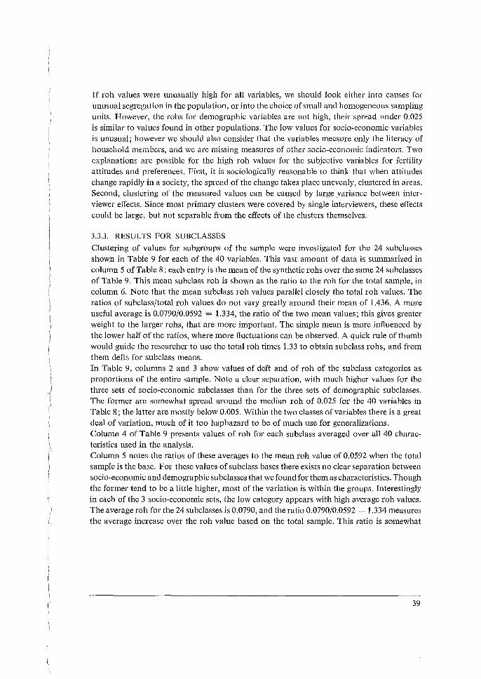
If roh values were unusually high for all variables, we should look either into causes for unusual segregation in the population, or into the choice of small and homogeneous sampling units. However, the rahs for demographic variables are not high, their spread under 0.025 is similar to values found in other populations. The low values for socio-economic variables is unusual; however we should also consider that the variables measure only the literacy of household men-ibers, and we are missing measures of other socio-economic indicators. Tv10 explanations are possible for the high roh values for the subjective variables for fertility attitudes and preferences. First, it is sociologically reasonable to think that when attitudes change rapidly in a society, the spread of the change takes place unevenly, clustered in areas. Second, clustering of the measured values can be caused by large .variance between inter­viewer effects. Since most primary clusters were covered by single interviewers, these effects could be large, but not separable from the effects of the clusters themselves.

3.3.3. RESULTS FOR SUBCLASSES

Clustering of values for subgroups of the sample were investigated for the 24 subclasses shown in Table 9 for each of the 40 variables. This vast amount of data is summarized in column 5 of Table 8 : each entry is the mean of the synthetic robs over the same 24 subclasses of Table 9. This mean subclass roh is shown as the ratio to the roh for the total sample, in column 6. Note that the mean subclass roh values parallel closely the total roh values. The ratios of subclass/total roh values do not vary greatly around their mean of 1.436. A more useful average is 0.0790/0.0592 = 1.334, the ratio of the two mean values; this gives greater weight to the larger rahs, that are more important. The simple mean is more influenced by the lower half of the ratios, where more fluctuations can be observed. A quick rule of thumb would guide the researcher to use the total roh times 1.33 to obtain subclass rahs, and from them defts for subclass means. In Table 9, columns 2 and 3 show values of deft and of roh of the subclass categories as proportions of the entire sample. Note a clear separation, with much higher values for the three sets of socio-economic subclasses than for the three sets of demographic subclasses. The former are somewhat spread around the median roh of 0.025 for the 40 variables in Table 8; the latter are mostly below 0.005. Within the two classes of variables there is a great deal of variation, much of it too haphazard to be of much use for generalizations. Column 4 of Table 9 presents values of roh for each subclass averaged over all 40 charac­teristics used in the analysis. Column 5 notes the ratios of these averages to the mean roh value of 0.0592 when the total sample is the base. For these values of subclass bases there exists no clear separation between socio-economic and demographic subclasses that we found for them as characteristics. Though the former tend to be a little higher, most of the variation is within the groups. Interestingly in each of the 3 socio-economic sets, the low category appears with high average roh values. The average roh for the 24 subclasses is 0.0790, and the ratio 0.0790/0.0592 = 1.334 measures the average increase over the rob value based on the total sample. This ratio is somewhat

39

higher for the 12 socio-economic subclasses than for the 12 demographic subclasses, 1.49 versus 1.17; the difference seems mainly due to only the three low socio-economic subclasses.

3.3.4. RESULTS FOR SUBCLASS MEAN DIFFERENCES

Subclass means are usually used for comparisons (r - r') between subclass means. We have 1.:umputed synthetic roh values for 2 pairs in each set of 4 subclasses; hence 2 x 6 = 12 comparisons, for each of the 40 variables. The means over the 12 values are shown in column 6 of Table 8. These synthetic rohd values are substantially lower than the corresponding subclass values. The individual ratios (not shown) of values in column 6 to column 4 vary considerably around their average of 0.095. A better average is the ratio of means: 0.00652/ 0.0790 = 0.083. The individual ratios range mostly from 0.30 to 0.00, except for some trivial cases near the bottom of the table, where negative values appear. We have also found in many other studies positive but smaller effects for differences than for the corresponding subclasses. In this study the reduction of effects seems more drastic than usual: the effects of covariance from clustering seem unusually strong. Consequently, the design effects of clustering on differences, though still present, are considerably reduced. In column 6 of Table 9 are shown synthetic rah values for differences of pairs of subclass means. Again each of the 12 entries represents an average over the 40 variables of Table 8. Note the great reductions in design effects due to positive covariances in clusters; the ratios of the average rahs is 0.0064/0.0790 = 0.081. Again the socio-economic subclasses have higher values of rahs for the differences than the demographic subclasses; 0.0110 versus 0.0019 for averages. Furthermore, the ratios to subclass rahs seemhigherin the former group than in the latter: 0.0110/0.0884 = 0.124 versus 0.0019/0.0695 = 0.027.

40

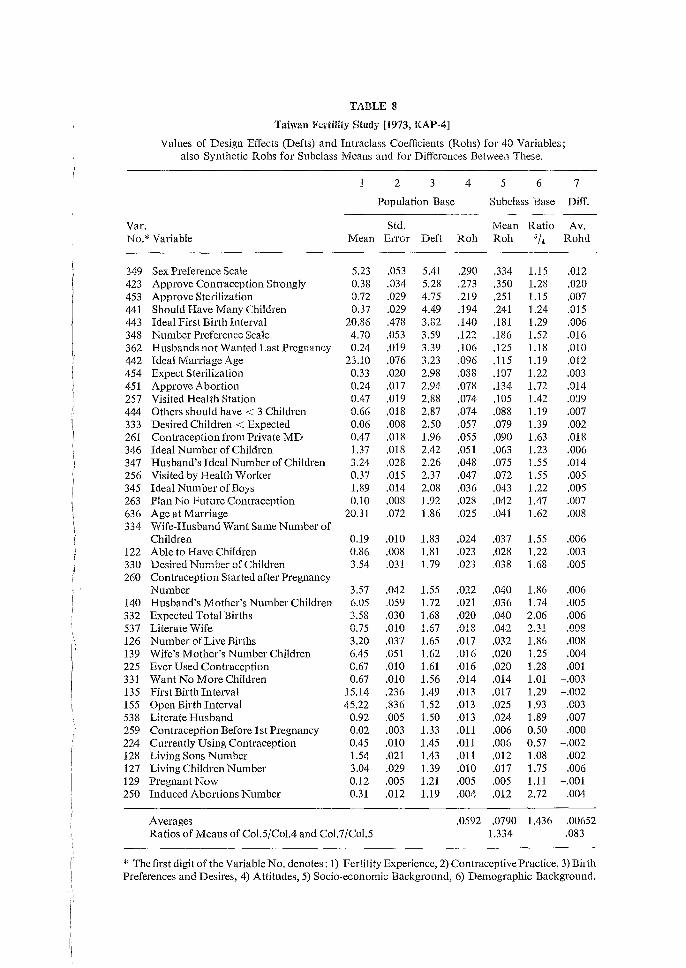
TABLE 8

Taiwan Fertility Study [1973, KAP-4]

Values of Design Effects (Defts) and Intraclass Coefficients (Rohs) for 40 Variables; also Synthetic Rohs for Subclass Means and for Differences Between These.

2 3 4 5 6 7

Population Base Subclass Base Diff.

Var. Std. Mean Ratio Av. No.* Variable Mean Error Deft Roh Roh 5/4 Rohd

349 Sex Preference Scale 5.23 .053 5.41 .290 .334 1.15 .012 423 Approve Contraception Sh·ongly 0.38 .034 5.28 .273 .350 1.28 .020 453 Approve Stedlization 0.72 .029 4.75 .219 .251 1.15 .007 441 Should Have Many Children 0.37 .029 4.49 .194 .241 1.24 .015 443 Ideal First Birth Interval 20.86 .478 3.82 .140 .181 1.29 .006 348 Number Preference Scale 4.70 .053 3.59 .122 .186 1.52 .016 362 Husbands not Wanted Last Pregnancy 0.24 .019 3.39 .106 .125 1.18 .010 442 Ideal Marriage Age 23.10 .076 3.23 .096 .115 1.19 .012 454 Expect Sterilization 0.33 .020 2.98 .088 .107 1.22 .003 451 Approve Abortion 0.24 .017 2.94 .078 .134 1.72 .014 257 Visited Health Station 0.47 .019 2.88 .074 .105 1.42 .0'.)9 444 Others should have < 3 Children 0.66 .018 2.87 .074 .088 1.19 .007 333 Desired Children < Expected 0.06 .008 2.50 .057 .079 1.39 .002 261 Contraception from Private MD 0.47 .018 1.96 .055 .090 1.63 .018 346 Ideal Number of Children 1.37 .018 2.42 .051 .063 1.23 .006 347 Husband's Ideal Number of Children 3.24 .028 2.26 .048 .075 1.55 .014 256 Visited by Health Worker 0.37 .015 2.37 .047 .072 1.55 .005 345 Ideal Number of Boys 1.89 .014 2.08 .036 .043 1.22 ,005 263 Plan No Future Contraception 0.10 .008 1.92 .028 .042 1.47 .007 636 Age at Marriage 20.31 .072 1.86 .025 .041 1.62 .008 334 Wife-Husband Want Same Number of

Children 0.19 .010 1.83 .024 .037 1.55 .006 122 Able to Have Children 0.86 .008 1.81 .023 .028 1.22 .003 330 Desired Number of Children 3.54 .031 1.79 ,02.3 .038 1.68 .005 260 Contraception Started after Pregnancy

Number 3.57 .042 1.55 .022 .040 1.86 .006 140 Husband's Mother's Number Children 6.05 .059 1.72 .021 .036 1.74 .005 332 Expected Total Births 3.58 .030 1.68 .020 .040 2.06 .006 537 Liieraie Wife 0.75 .010 1.67 f\1 Q

oV.LV .042 2.31 .008 126 Number of Live Births 3.20 .037 1.65 .017 .032 1.86 .008 139 Wife's Mother's Number Children 6.45 .051 1.62 .016 .020 1.25 .004 225 Ever Used Contraception 0.67 ,010 1.61 .016 .020 1.28 .001 331 Want No More Children 0.67 .010 1.56 .014 .014 1.01 -.003 135 First Birth Interval 15.14 .236 1.49 .013 .017 1.29 -.002 155 Open Birth Interval 45.22 .836 1.52 .013 .025 1.93 .003 538 Literate Husband 0.92 .005 1.50 .013 .024 1.89 .007 259 Contraception Before 1st Pregnancy 0.02 .003 1.33 .011 .006 0.50 .000 224 Currently Using Contraception 0.45 .010 1.45 .011 .006 0.57 -.002 128 Living Sons Number 1.54 .021 1.43 .011 .012 1.08 .002 127 Living Children Number 3.04 .029 1.39 .010 .017 1.75 .006 129 Pregnant Now 0.12 .005 1.21 .005 .005 1.11 -.001 250 Induced Abortions Number 0.31 .012 1.19 .004 .012 2.72 .004

Averages .0592 .0790 1.436 .00652 Ratios of Means of Col.5/Col.4 and Col.7 /Col.5 1.334 .083

* The first digit of the Variable No. denotes: 1) Fertility Experience, 2) Contraceptive Practice, 3) Birth Preferences and Desires, 4) Attitudes, 5) Socio-economic Background, 6) Demographic Background.

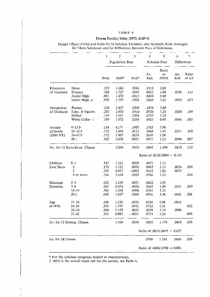
TABLE 9

Taiwan Fertility Study [1973, KAP-4]

Design Effects (Defts) and Rohs for 24 Subclass Variables; also Synthetic Rohs Averaged for These Subclasses and for Differences Between Pairs of Subclasses.

2 3 4 5 6 7

Population Base Subclass Base Differences

Ratio Av. to Av. Ratio

Prop. Deft* Roh* Roh .0592t Roh of 6/4

Education None .255 1.684 .0186 .1212 2.05 of Husband Primary .548 1.727 .0201 .0615 1.04 .0101 .111

Junior High .081 1.453 .0112 .0410 0.69 Senior High + .070 1.739 ,0205 .0969 1.64 .0053 .077

Occupation Farmer .219 2.437 .0509 .1474 2.49 of Husband Lahr. & Opertv. .202 2.002 .0310 .0726 1.23 .0208 .189

Skilled .159 1.951 .0289 .0733 1.24 White Collar + .359 1.872 .0258 .0525 0.89 .0041 .065

Income 0-23.9 .154 4.171 .1987 .1765 2.98 of family 24-35.9 .172 1.445 .0132 .0868 1.47 .0211 .160 (1000 NT) 36-47.9 .172 1.807 .0274 .0639 1.08

48+ .303 2.476 .0621 .0671 1.13 .0044 .067

Av. for 12 Socio-Econ. Classes 2.064 .0424 .0884 1.494 .0110 .112

Ratio of .0110/.0084 = 0.124

Children 0-1 .147 1.221 .0050 .0671 1.13 Ever Born 2 .172 1.122 .0026 .0667 1.13 .0036 .054

3 .239 0.987 -.0002 .0613 1.04 .0025 4 or more .396 1.429 .0105 .0766 l.2S .036

Marriage 0--4 .228 1.139 .0031 .0622 1.05 Duration 5-9 .267 0.874 -.0024 .0647 1.09 .0031 .049

10-19 .386 1.038 .0008 .0741 1.25 20+ .058 1.037 .0008 .0936 1.58 -.OUOl -.OOi

Age 19-24 .189 1.150 .0032 .0554 0.94 .0014 of Wife 25-29 .252 1.187 .0041 .0715 1.21 .022

30-34 .260 1.169 .0037 .0678 1.14 .0006 35--42 .255 0.892 -.0021 .0733 1.24 .008

Av. for 12 Demog. Classes 1.104 .0024 .0695 1.174 .0019 .028

Ratio of .0019/.0695 = 0.027

Av. for 24 Classes .0790 1.334 .0064 .070

Ratio of .0064/.0790 = 0.081

* For the subclass categories treated as characteristics. t .0592 is the overall mean roh for the sample, see Table 8.

i'

I

3.4 MALAYSIA: SURVEY OF ACCEPTORS OF FAMILY PLANNING (1969) (TABLES 10-12)

3.4.1. DESCRIPTION OF THE SAMPLE**

This sample was selected, with equal probability, from the list of 55,000 acceptors of two large family planning programmes. The survey, conducted in 1969, yielded 2590 interviews. In the rural strata 1,559 women (60 %) came from mukims (administrative units), an average of 70.86 women per mukim. The urban strata accounted for 430 women (17 %) and the metropolitan strata for 611 (23 %) ; here women were selected individually, which accounts for design effects near 1 for them.

3.4.2. DESIGN EFFECTS

In Table 10 values of deft are shown for the total sample and for the three large strata in which separate samples were selected: metropolitan, urban and rural. The rural sample shows large deft values. These are also reflected in the total sample, of which 60 per cent is rural. In the metropolitan and urban areas we can accept deft = 1 as the average, and the variations about it as dominated by just random fluctuations. The rather large fluctuations are due to using, for convenience, few combined units for variance computations. The negligible design effect is due to lack of clustering in these two strata, where the acceptors were selected individually from lists of names. Theoretically the average of deft = 1 may combine small gains from geographical stratification and small losses from clustering. Hence the average value of deft = 1 is more accurate for the metropolitan and urban strata than the specific deft values for variables, because these are due mostly to random fluctuations. On hindsight, we could have omitted these computations. The large subclass for pill users (91 per cent) shows large values of deft. The small subclass for loop users (2 per cent) is widely scattered and we may accept deft = 1 for it, with random fluctuations. Values of deft are also shown for differences between these subclasses. The metropolitan­urban differences naturally also fluctuate around deft = 1, as their two independent com­ponents do. The metropolitan-rural and urban-rural differences show increased deft values, due to the rural component of the pairs. The effects are less than in the total, because in the comparisons the rural 'weight' is only one half; they average 1.37 and 1.30 as against 1.61. The pill-loop comparisons show slight effects, due to the pill component. The effects are reduced by covariances arising from both components coming from the same clusters. Let us now look at the 29 variables, the rows of Table 10. These are listed by decreasing values of deft in the rural column; these also give closely decreasing values in the total column. The values in this column should help the reader find useful regularities in accord with the substantive nature of the variables listed. The first variable is an outlier: For the rural sample the intraclass correlation is very high, because each rural place had either an NFPB clinic or an FP A clinic, where the women

** For details see Tan, B. A., and Takeshita, J. Y., [1970], 'An Interim Report on the 1969 West Malaysian Family Planning Acceptor Follow-up Survey,' Paper No. 5 in Proceedings of the Combined Conference on Evaluation of Malaysia National Family Planning Programme and East Asia Population Programmes, 18-25 March, Kuala Lumpur: National Family Planning Board of Malaysia, pp. 155-229. Kish, L. and Takeshita, 'Sampling Errors in a Family Planning Survey Malaysia,' [1974], Paper for Annual Meeting of the Population Association of America.

43

usually went. If we had known about this exclusiveness we could have used it for stratifi­cation. The second variable is also an outlier: it shows that in most rural areas ethnic groups in this population (or at least the women going to the clinics) tend to cluster, as Malay, or Chinese, or Indian. This design effect also can be used for, and reduced by, stratification in situations where the information is available for all or most places. The other 27 variables may no\V be examined for more customary sources of variation. They range in deft values for rural places from 1.03 to 2.64, approximately a sevenfold range for deft 2 and the variance. Perhaps we are most interested in items about fertility and contraception, coded 1 and 2. These have deft values in rural places from 1.12 to 2.17; factors from 1.3 to 4.7 for the variances.

3.4.3. VALUES OF ROH

Table 11 contains synthetic values of roh computed from the deft values of Table 10. They are ordered again in decreasing size. The value for the rural sample was computed as roh = (deft 2 - 1) / 69.86, where 1559/22 =

70.86 is the average cluster size in the 22 mukims that comprise the rural sample. The synthetic rah incorporates whatever effects inequalities of size have on the deft values and variances. We need roh values for the total sample for their own sake and for comparisons with subclasses crossing across the urban-rural strata. Vve saw, in discussions of Table 10, that there was effectively no clustering in the urban and metro strata. Hence we used a corre­sponding model [see section 2.3] that yielded a = 22/(0.60 2 + 0.40 x 22/2590) = 60.16 pseudoclusters, where 0.60 is the proportion rural. This yields 2590/60.16 = 43.05 as the synthetic cluster size b. This jj with the synthetic values of rah would have the same design effect 1 + roh (5- 1) as the combination of rural clustering for 0.60 and urban scattering for 0.40 had in reality. The synthetic total roh values were computed from the total deft values as (deft 2

- 1)/42.05. They show good agreement with the rural roh values. Differences do not appear important and the two averages are 0.0463 for rural values and 0.0453 for the synthetic total values. Most oftheroh values, and the most important, are in the range 0.02 to 0.05, with the median and mean near 0.035 without the two large outliers. Now we come to subclasses, computed for 14 variables, as shown in column 4. Each is the average over 22 subclasses of rohs, computed from deft values as roh = (deft 2 - 1) / (n/60.16 - 1). They resemble, with fluctuations, the corresponding values from the total sample, but they are slightly higher. The ratio of the two average rohs for 14 variables (roh8 /roh1) of subclasses over totals is 0.0554/0.0277 = 2.00. However, the 22 subclasses confuse two rather distinct types, we find; and in Table 12 we separate the top 6 pairs from the last 5 pairs. These 5 pairs of subclasses appear a priori close to being crnss-dasses, that is, subclasses that cut across the clusters of selection. On the

44

contrary, the top 6 pairs of subclasses are more prone to be bound to clusters; and, in fact, they have among the highest values of roh (nos. I, 2, 3 and 6) in column 2 of Table 10. For the 10 cross-classes the average roh is 0.0318, and this has a ratio of only 0.0318/0.0277 =

1.15 to the average of 0.0277 for the total rohs in column 3. Further, we also computed synthetic roh measures for the 11 differences between subclass means. These incorporate the effects of covariances between the pairs of means; by com­paring them to the corresponding subclass roh's we measure the effects of the covariances. We note that the average 0.0356/0.0554 = 0.64 measures the average reduction due to covariances in the 11 pairs. Again we treat separately in column 7 the 5 pairs of cross-classes. Here the reduction due to covariance is much greater; the ratio of the averages is 0.0067/0.0318 = 0.21. Table 12 is complementary to Table 11 in summarizing the analysis of (11 x 2) x 14 values ofroh. Table 11 in column 4 and in column 6 gave the marginal values for the 14 variables, each averaged over the 22 subclasses and 11 differences. Table 12 gives the marginals that average over the 14 variables for each of the 22 subclasses and the 11 differences. Note the large difference between the top 6 pail's and the bottom 5 pairs. The ratios of averages of subclass robs to total rohs are 0.0750/0.0277 = 2.71 and 0.0318/0.0277 = 1.15 respectively. Ratios of rohs for differences to subclass robs are 0.0597 /0.0750 = 0.80 and 0.0067/0.0318 = 0.21 respectively. Results for the 5 pairs of cross-class robs are consistent with similar results from other surveys: the ratio of 1.15 for cross-classes over total and the ratio of 0.21 for differences over cross-classes. The ratios of 2.71 and 0.80 for the other 6 pairs are distinctly different, and should be considered separately.

45

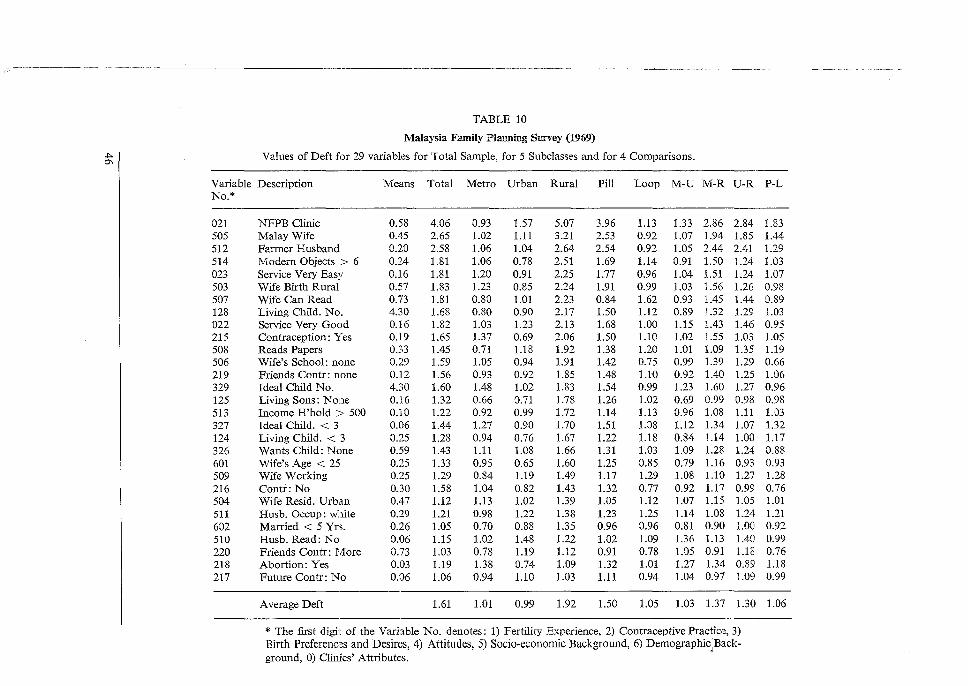
TABLE 10

Malaysia Family Planning SW"vey (1969)

""" Values of Deft for 29 variables for Total Sample, for 5 Subclasses and for 4 Comparisons. °'

Variable Description Means Total Metro Urban Rural Pill Loop M-U M-R U-R P-L No.*

021 NFPB Clinic 0.58 4.06 0.93 1.57 5.07 3.96 1.13 1.33 2.86 2.84 1.83 505 Malay Wife 0.45 2.65 1.02 1.11 3.21 2.53 0.92 1.07 1.94 1.85 1.44 512 Farmer Husband 0.20 2.58 1.06 1.04 2.64 2.54 0.92 1.05 2.44 2.41 1.29 514 Modern Objects > 6 0.24 1.81 1.06 0.78 2.51 1.69 1.14 0.91 1.50 1.24 1.03 023 Service Very Easy 0.16 1.81 1.20 0.91 2.25 1.77 0.96 1.04 1.51 1.24 1.07 503 Wife Birth Rural 0.57 1.83 1.23 0.85 2.24 1.91 0.99 1.03 1.56 1.26 0.98 507 Wife Can Read 0.73 1.81 0.80 1.01 2.23 0.84 1.62 0.93 1.45 1.44 0.89 128 Living Child. No. 4.30 1.68 0.80 0.90 2.17 1.50 1.12 0.89 1.32 1.29 1.03 022 Service Very Good 0.16 1.82 1.03 1.23 2.13 1.68 1.00 1.15 1.43 1.46 0.95 215 Contraception: Yes 0.19 1.65 1.37 0.69 2.06 1.50 1.10 1.02 1.55 1.03 1.05 508 Reads Papers 0.33 1.45 0.71 1.18 1.92 1.38 1.20 1.01 1.09 1.35 1.19 506 Wife's School: none 0.29 1.59 1.05 0.94 1.91 1.42 0.75 0.99 1.39 1.29 0.66 219 Friends Contr: none 0.12 1.56 0.93 0.92 1.85 1.48 1.10 0.92 1.40 1.25 1.06 329 Ideal Child No. 4.30 1.60 1.48 1.02 1.83 1.54 0.99 1.23 1.60 1.27 0.96 125 Living Sons: None 0.16 1.32 0.66 0.71 1.78 1.26 1.02 0.69 0.99 0.98 0.98 513 Income H'hold > 500 0.10 1.22 0.92 0.99 1.72 1.14 1.13 0.96 1.08 1.11 1.03 327 Ideal Child. < 3 0.06 1.44 1.27 0.90 1.70 1.51 1.08 1.12 1.34 1.07 1.32 124 Living Child. < 3 0.25 1.28 0.94 0.76 1.67 1.22 1.18 0.84 1.14 1.00 1.17 326 Wants Child: None 0.59 1.43 1.11 1.08 1.66 1.31 1.03 1.09 1.28 1.24 0.88 601 Wife's Age < 25 0.25 1.33 0.95 0.65 1.60 1.25 0.85 0.79 1.16 0.93 0.93 509 Wife Working 0.25 1.29 0.84 1.19 1.49 1.17 1.29 1.08 1.10 1.27 1.28 216 Contr: No 0.30 1.58 1.04 0.82 1.43 1.32 0.77 0.92 1.17 0.99 0.76 504 Wife Resid. Urban 0.47 1.12 1.13 1.02 1.39 1.05 1.12 1.07 1.15 1.05 1.01 511 Husb. Occup: white 0.29 1.21 0.98 1.22 1.38 1.23 1.25 1.14 1.08 1.24 1.21 602 Married< 5 Yrs. 0.26 1.05 0.70 0.88 1.35 0.96 0.96 0.81 0.90 1.00 0.92 510 Husb. Read: No 0.06 1.15 1.02 1.48 1.22 1.02 1.09 1.36 1.13 1.40 0.99 220 Friends Contr: More 0.73 1.03 0.78 1.19 1.12 0.91 0.78 1.05 0.91 1.18 0.76 218 Abortion: Yes 0.03 1.19 1.38 0.74 1.09 1.32 1.01 1.27 1.34 0.89 1.18 217 Future Contr: No 0.06 1.06 0.94 1.10 1.03 1.11 0.94 1.04 0.97 1.09 0.99

Average Deft 1.61 1.01 0.99 1.92 1.50 1.05 1.03 1.37 1.30 1.06

* The first digit of the Variable No. denotes: I) Fertility Experience, 2) Contraceptive Practice, 3) Birth Preferenci~s and Desires, 4) Attitudes, 5) Socio-economic Background, 6) Demographic;Back-ground, 0) Clinics' Attributes.

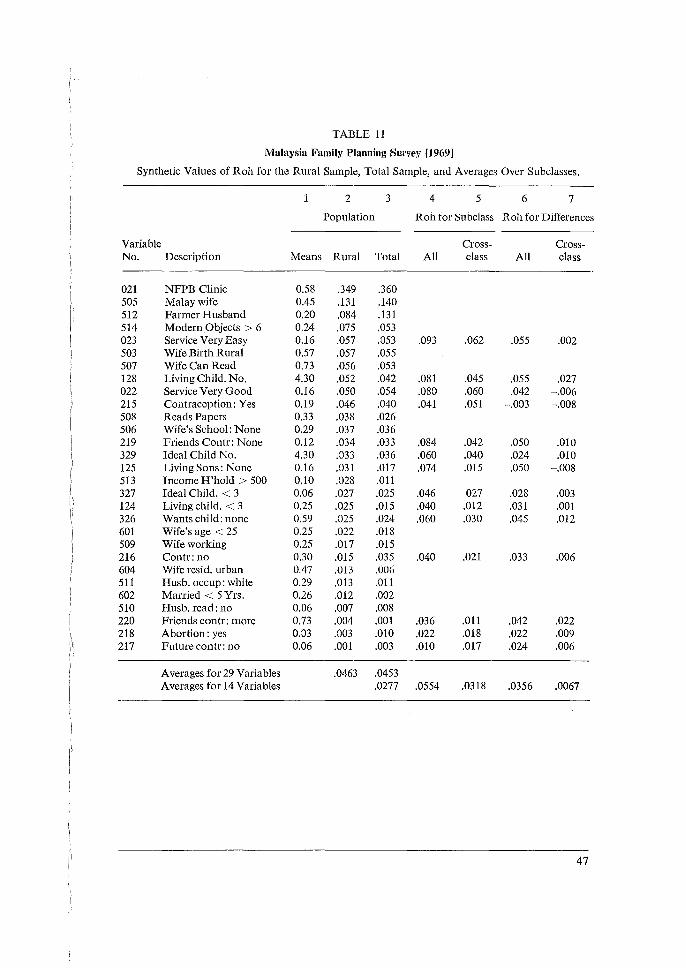
TABLE 11

Malaysia Family Planning Survey (1969]

Synthetic Values of Roh for the Rural Sample, Total Sample, and Averages Over Subclasses.

2 3 4 5 6 7

Population Roh for Subclass Roh for Differences

Variable Cross- Cross-No. Description Means Rural Total All class All class

021 NFPB Clinic 0.58 .349 .360 505 Malay wife 0.45 .131 .140 512 Farmer Husband 0.20 .084 .131 514 Modern Objects> 6 0.24 .075 .053 023 Service Very Easy 0.16 .057 .053 .093 .062 .055 .002 503 Wife Birth Rural 0.57 .057 .055 507 Wife Can Read 0.73 .056 .053 128 Living Child. No. 4.30 .052 .042 .081 .045 .055 .027 022 Service Very Good 0.16 .050 .054 .080 .060 .042 -.006 215 Contraception: Yes 0.19 .046 .040 .041 .051 -.003 -.008 508 Reads Papers 0.33 .038 .026 506 Wife's School: None 0.29 .037 .036 219 Friends Con tr: None 0.12 .034 .033 .084 .042 .050 .oIO 329 Ideal Child No. 4.30 .033 .036 .060 .040 .024 .010 125 Living Sons: None 0.16 .031 .017 .074 .015 .050 -.008 513 Income H'hold > 500 0.10 .028 .011 327 Ideal Child. < 3 0.06 .027 .025 .046 027 .028 .003 124 Living child. < 3 0.25 .025 .015 .040 .012 .031 .001 326 Wants child: none 0.59 .025 .024 .060 .030 .045 .012 601 Wife's age < 25 0.25 .022 .018 509 Wife working 0.25 .017 .015 216 Contr: no 0.30 .015 .035 .040 .021 .033 .006 604 Wife resid. urban 0.47 .013 .006 511 Husb. occup: white 0.29 .013 .011 602 Married < 5 Yrs. 0.26 .012 .002 510 Husb. read: no 0.06 .007 .008 220 Friends contr: more 0.73 .004 .001 .036 .011 .042 .022 218 Abortion: yes 0.03 .003 .010 .022 ,018 .022 .009

r, 217 Future con tr: no 0.06 .001 .003 .010 .017 .024 .006

Averages for 29 Variables .0463 .0453 I

I Averages for 14 Variables .0277 .0554 .0318 .0356 .0067

I

47

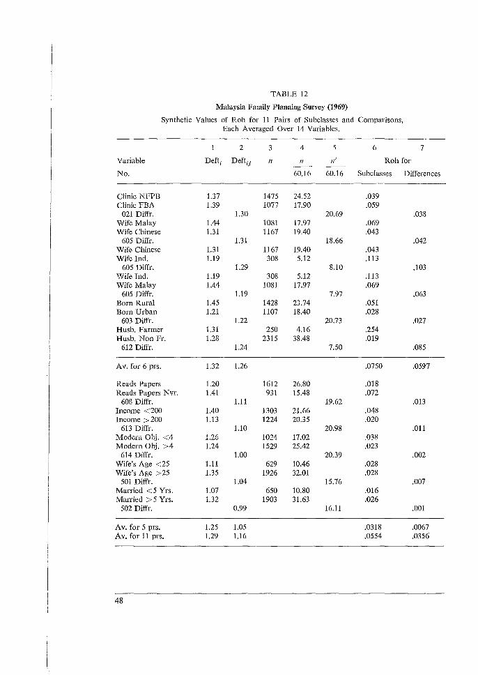
TABLE 12

Malaysia Family Planning Survey (1969)

Synthetic Values of Roh for 11 Pairs of Subclasses and Comparisons, Each Averaged Over 14 Variables.

2 3 4 5 6 7

Variable Deft; Deftij II 11 11' Roh for

No. 60.16 60.16 Subclasses Differences

Clinic NFPB 1.37 1475 24.52 .039 Clinic FBA 1.39 1077 17.90 .059

021 Diffr. 1.30 20.69 .038 Wife Malay 1.44 1081 17.97 .069 Wife Chinese 1.31 1167 19.40 .043

605 Diffr. 1.31 18.66 .042 Wife Chinese 1.31 1167 19.40 .043 Wife Ind. 1.19 308 5.12 .113

605 Diffr. 1.29 8.10 .103 Wife Ind. 1.19 308 5.12 .113 Wife Malay 1.44 1081 17.97 .069

605 Diffr. 1.19 7.97 .063 Born Rural 1.45 1428 23.74 .051 Born Urban 1.21 1107 18.40 .028

603 Diffr. 1.22 20.73 .027 Husb. Farmer 1.31 250 4.16 .254 Husb. Non Fr. 1.28 2315 38.48 .019

612 Diffr. 1.24 7.50 .085

Av. for 6 pm. 1.32 1.26 .0750 .0597

Reads Papers 1.20 1612 26.80 ,018 Reads Papers Nvr. 1.41 931 15.48 .072

608 Diffr. 1.11 19.62 .013 Income <200 1.40 1303 21.66 .048 Income >200 1.13 1224 20.35 .020

613 Diffr. 1.10 20.98 .011 !vfodern Obj. <4 1.26 1024 17.02 .038 Modern Obj. >4 1.24 1529 25.42 .023

614 Diffr. 1.00 20.39 .002 Wife's Age <25 1.11 629 10.46 .028 Wife's Age > 25 1.35 1926 32.01 .028

501 Diffr. 1.04 15.76 .007 Married <5 Yrs. 1.07 650 10.80 .016 MalTied >5 Yrs. i.32 1903 31.63 .026

502 Diffr. 0.99 16.11 .001

Av. for 5 prs. 1.25 1.05 .0318 .0067 Av. for 11 prs. 1.29 1.16 .0554 .0356

48

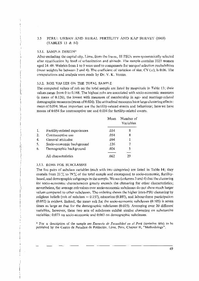
3.5 PERU: URBAN Al\TD RURAL FERTILITY AND KAP SURVEY (1969) (TABLES 13 & 14)

3.5.1. SAMPLE DESIGN* After excluding the capital city, Lima, from the frame, 88 PSUs were systematically selected after stratification by level of urbanization and altitude, The sample contains 3327 women aged 14-49. Weights from 1 to 9 were used to compensate for unequal selection probabilities (most weights lie between 2 and 4). The coefficient of variation of size, CV (x ), is 0.06. The computations and analysis were made by Dr. V. K. Verma.

3.5.2. ROH VALUES ON THE TOTAL SAMPLE The computed values of rob on the total sample are listed by magnitude in Table 13 ; their values range from 0 to 0.168. The highest robs are associated with socio-economic measures (a mean of 0.126), the lowest with measures of membership in age- and marriage-related demographic measures (mean of 0.024). The attitudinal measures have large clustering effects: mean of 0.094. Most important are the fertility-related events and behaviour; here we have means of 0.054 for contraceptive use and 0.034 for fertility-related events.

Mean Number of Variables

1. Fertility-related experiences .034 8 2. Contraceptive use .054 8 4. General attitudes .094 5. Socio-economic background .126 7 6. Demographic background .024 5

All characteristics .062 29

3.5.3. ROHS FOR SUBCLASSES The five pairs of subclass variables (each with two categories) are listed in Table 14; they contain from 21 % to 79 % of the total sample and correspond to socio-economic, fertility­based, and demographic subgroups in the sample. We see (columns 3 and 4) that the clustering for socio-economic characteristics greatly exceeds the clustering for other characteristics; nevertheless, the average rob values over socio-economic subclasses do not show much larger values compared to other subclasses. The ordering shows the higher intra-PSU clustering by religious beliefs (rob of subclass = 0.157), education (0.107), and labour-force participation (0.052) is evident. Indeed, the mean roh for the socio-economic subclasses (0.105) is seven times as large as that for the demographic subclasses (0.015). Averaging over 20 different variables, however, these two sets of subclasses exhibit similar clustering on substantive variables: 0.073 on socio-economic and 0.063 on demographic subclasses.

* For a description of the sample see Encuesta de Fecundidad en el Peni (tentative title) to be published by the Centro de Estudios de Poblaci6n, Lima, Peru, Chapter II, "Methodology".

49

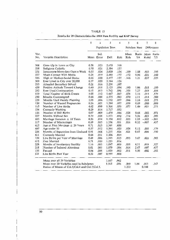
TABLE 13

Results for 29 Characteristics for 1969 Peru Fertility aml KAP Survey

2 3 4 5 6 7 8

Population Base Subclass Base Differences

Var. Std. Mean Ratio Mean Ratio No. Variable Description Mean Error Deft Roh Roh 5/4 Rohd 7/5

508 Grew Up in Town or City 0.58 .023 2.670 .168 538 Religious Catholic 0.70 .021 2.584 .157 231 Intercourse More than Once a Week 0.55 .024 2.020 .156 .169 1.08 .033 .195 537 Much Contact With Media 0.28 .019 2.480 .137 .132 0.96 .021 .160 536 High or Medium Social Status 0.66 .020 2.477 .137 .166 1.21 .037 .223 509 Ever Lived in City over 20,000 0.37 .020 2.364 .126 535 Attended Secondary School 0.21 .016 2.238 .107 439 Positive Attitude Toward Change 0.40 .018 2.125 .094 .100 1.06 .018 .180 232 Ever Used Contraception 0.15 .013 1.762 .081 .103 1.27 .019 .184 119 Total Number of Birth Events 5.05 .112 1.667 .067 .078 1.16 .014 .179 230 Months Contracepted 0.66 .088 1.575 .063 .070 1.11 .014 .200 229 Months Used Family Planning 1.05 .106 1.532 .057 .066 1.16 .ol8 .273 120 Number of Wasted Pregnancies 0.26 .021 1.584 .057 .039 0.69 .000 .000 115 Number of Live Births 4.62 .099 1.566 .055 .077 1.40 .021 .273 534 Currently Working 0.29 .014 1.717 .052 116 Number of Still Births 0.07 .009 1.470 .044 .028 0.64 .002 .071 227 Months Without Sex 0.19 .028 1.313 .032 .114 3.56 .023 .202 613 Marriage Duration :S 10 Years 0.56 .014 1.354 .032 .033 1.03 -.002 -.061 117 Number of Miscarriages 0.19 .015 1.356 .031 .016 0.52 -.007 -.437 612 Age at First Marriage :S 20 Years 0.71 .013 1.341 .030 607 Age under 30 0.57 .012 1.386 .025 .028 1.12 .005 .179 226 Months of Separation from Husband 0.91 .066 1.255 .024 .021 0.87 .004 .190 611 Currently Married 0.64 .011 1.304 .019 124 Live Births per Year of Marriage 0.49 .006 1.183 .ol5 .055 3.67 .021 .382 612 Ever Married 0.71 .DiO 1.229 .014 228 Months of Involuntary Sterility 1.16 .083 1.097 .009 .055 6.11 .018 .327 218 Number oflnduced Abortions 0.01 .003 1.079 .006 .016 2.67 .007 .437 133 Fecund 0.84 .008 1.029 .002 .011 5.50 .002 .182 121 Live Births Past Year 0.22 .007 0.999 .000

Mean over all 29 Variables 1.647 .062 Mean over 20 Variables used in Subclasses 1.565 .056 .069 1.84 .013 .167 Ratios of Means of Col.5/Col.4 and Col.7/Col.5. 1.232 0.188

50

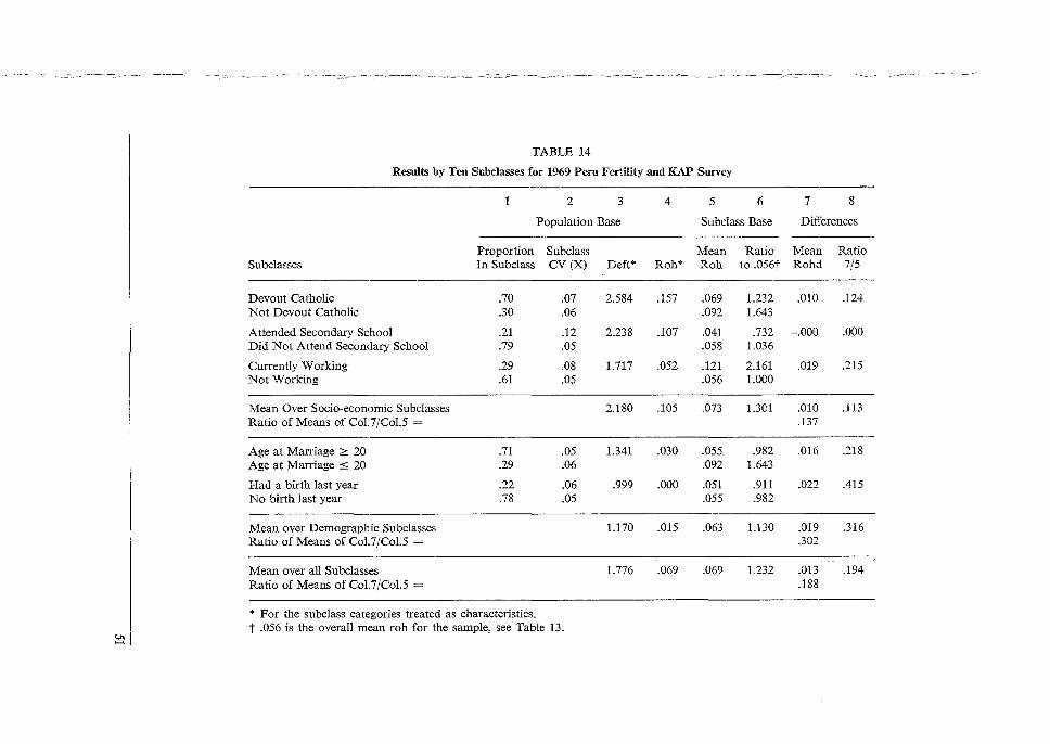
TABLE 14

Results by Ten Subclasses for 1969 Peru Fertility and KAP Survey

1 2 3 4 5 6 7 8

Population Base Subclass Base Differences

Proportion Subclass Mean Ratio Mean Ratio Subclasses In Subclass CV(X) Deft* Roh* Roh to .056t Rohd 7/5

Devout Catholic .70 .07 2.584 .157 .069 1.232 .010 .124 Not Devout Catholic .30 .06 .092 1.643

Attended Secondary School .21 .12 2.238 .107 .041 .732 -.000 .000 Did Not Attend Secondary School .79 .05 .058 1.036

Currently Working .29 .08 1.717 .052 .121 2.161 .019 .215 Not Working .61 .05 .056 1.000

Mean Over Socio-economic Subclasses 2.180 .105 .073 1.301 .010 .113 Ratio of Means of Col.7/Col.5 = .137

Age at Marriage <:: 20 .71 .05 1.341 .030 .055 .982 .016 .218 Age at Marriage s 20 .29 .06 .092 1.643

Had a birth last year .22 .06 .999 .000 .051 .911 .022 .415 No birth last year .78 .05 .055 .982

Mean over Demographic Subclasses 1.170 .015 .063 1.130 .019 .316 Ratio of Means of Col.7 /Col.5 = .302

Mean over all Subclasses 1.776 .069 .069 1.232 .013 .194 Ratio of Means of Col.7 /Col.5 = .188

* For the subclass categories treated as characteristics. t .056 is the overall mean roh for the sample, see Table 13.

~

Column 5 of Table 13 presents the average roh over the 10 subclasses for each of the twenty variables examined. These values, as we have consistently seen in the other samples, are somewhat higher than rahs for the same variables on the total sample. Column 6 shows that this ratio varies considerably over the twenty variables, with most variability occurring among variables with small values of roh. The ratio of mean subclass roh over the twenty variables (0.069) to the mean roh on the total sample (0.056) is 1.23.

3.5.4. ROHS FOR SUBCLASS DIFFERENCES

Columns 7 and 8 of Table 13 present results for the average rohd of differences. These values are much smaller (mean = 0.013) than robs on the total sample (mean = 0.056) or on the same subclasses (mean = 0.069). This reduction is related to the positive covariance of the two subclass means within PSUs. The ratio of the rohd for the difference to subclass roh varies over the 20 measures; a useful summary measure of the relationship is the ratio of the mean roh of the difference over all variables (0.013) to the mean subclass rob (0.069), which is 0.188.

3.6 UNITED STATES FERTILITY SURVEYS (TABLES 15-17)

For the United States we have assembled four different fertility studies, conducted in 1955, 1960, 1965, 1970, and several comparisons on similar variables can be made across the different years. The most complete analyses of sampling errors is performed on the 1970 data, where sampling variances both on whites and blacks were computed.

3.6.1. SAMPLE DESIGNS

The 1955 and 1960 studies of the Growth of the American Family (GAF) were based on essentially similar multistage area probability samples of private households in the U.S., conducted by the Institute for Social Research (University of Michigan). In addition to the 'self-representing' 12 largest metropolitan areas, 54 'other-representing' primary areas -SMSA's or counties - were selected from that many strata. Equal probability for every household in the U.S. was achieved through several stages of selection with probabilities proportional to size: primary area, place (city, town, or open country area), blocks, segments. Clusters averaging about 8 dwellings per block or rural segments yielded averages of about 3 eligible women. The 1955 sample yielded 2709 interviews with eligible women from 8305 households: white women, 18-39 married with husband present, and single women 18-24. From the 1960 sample, also of white women, the sampling error computations involve 2412 married women 18-39, from 8426 households. The synthetic numbers a of clusters and b of average cluster sizes were computed as follows.

52

For the 1955 study, where the proportion 1993/2709 of interviews came from the 54 primary areas, the rest mostly from blocks averaging about 3 interviews the

[(1993)

2 54 ( 1993)]-l a = 54

2709 + 3

2709 1 -

2709 = 54 [.5412 + .Gl58]-1 = 96.9,

and b = 2709/96.9 = 28.00. Similarly for the 1960 study, with 1709/2412 of the interviews coming from the 54 primary areas, we have

a = 54 [ G:~~) 2

+ 3 2~;2 ( 1 _ ~:~~) J1

= 54 [.5020 + .0196]-l = 103.5,

and b = 2412/103.5 = 23.3. Eligible respondents for the 1965 National Fertility Study were married white and non-white women, less than 55 years of age, living with their husbands; but only whites under 45 years of age were used for this analysis. Twenty-seven strata were defined by 9 geographical divi­sions and 3 population zones: cities of 50,000 or more population, areas in SMSA's not included in the first category, and non-metropolitan areas. This 9 x 3 categorization of the sampling frame was divided into 106 strata of approximately 500,000 households each. PS Us of contiguous census tracts and enumeration districts were formed, with an expected size of 10,000 households each. Eight PSUs (large metropolitan areas) were selected with cer­tainty; in the non-metropolitan group, 2 PSUs were selected per stratum, in the two other zones a single PSU was selected from each stratum. 148 clusters were used for sampling error purposes. 3767 white married women below 45 provided interviews for an average cluster size of 25 respondents. For the United States Fertility Study of 1970, using 1960 census materials, the 48 states were listed in continuous serpentine fashion to form 9 geographical strata. Within the states, listing of metropolitan areas by size and non-metropolitan counties by a geographical ordering formed six (6) distinct community size strata, which were divided into equal size zones of 940,000 households. Since these zones of940,000 were not permitted to cross the geographical/ community size strata, incomplete zones in some of the 6 x 9 = 54 strata were partly empty. Two PSUs of 10,000 contiguous households were selected by systematic sampling from each zone yielding 152 PSUs, 126 with some real households plus 26 of no real householdy. Within each PSU, 13 listing areas (blocks or census enumeration districts) of approximateld 50 housing units were selected systematically, listed, and an expected 18 households selectep from each listing area. In one-half of the selected households one married woman ages 14-44 years was selected only if she was black; in the other half one married woman aged 14-44 was selected per household regardless of race. Sampling errors were calculated utilizing all 152 PSUs paired into 76 strata. The vast majority of non-blacks are whites and we will refer to them as 'whites' in the following discussion.

53

3.6.2. ROHS ON THE ENTIRE SAMPLE

Table 15 presents means, <lefts, sample sizes, rohs and coefficients of variation for cluster size on variables whose sampling errors were calculated on at least three of the four U.S. studies for whites. The coefficients of variation of cluster size [CV (x)] range from 0.04 to 0.06, and these are well within limits of the utility of the variance estimate. Three of the variables have robs calculated in all four of the studies: fecundity, per cenl curnmlly using contraception, and the number of births expected. Generally, the homogeneity values for the 1965 and 1970 samples are larger than those for the 1955 and 1960 samples. For five similar variables in Table 15, the mean rohs are for 1960, 0.020; for 1965, 0.053; and for 1970, 0.038. We suspect that this is related to the unusually small PSU size of the latter two designs (approximately 10,000 households), which would force a tighter clustering of secondary selections within the PSUs. A more complete analysis (although more subject to sampling variation) can be made sepa­rately for the 1960 sample for whites, and for the 1970 samples for whites and blacks. Tables 16 and 17 present statistics of interest on variables from the three samples. But first some general remarks are useful. The values of roh seem to vary rather regularly across the five substantive groupings. The fertility experience and fertility preference variables are rather widely spread, but mostly among the lower magnitudes of rohs. Among these fertility variables the highest rohs in all three samples is for the mean number of live births. The contraception variables seem to have high minimum roh's, and fall in the middle of the distribution. The table below presents the mean roh's for the five different groupings we distinguished:

1960 No. of 1970 No. of Substantive Grouping of Fertility Variables Whites Var. Whites Blacks Var.

1. Fertility Experience .011 4 .019 .098 5 2. Contraceptive Practices .043 2 .029 .137 8 3. Preferences .025 2 .019 .142 6 4. Attitudes .051 .150 16

In all three samples fertility experiences have the lowest average rates of homogeneity (rohs) of the five variable types. General attitudes toward fertility-related experiences have higher rohs, averaging 0.051 in the white sample and 0.150 in the black sample. We suspect that these attitudinal measures may be more subject to the effects of interviewer differences (in delivery style, amount of probing, etc.), so that to the extent that sample elements in the same PSU were assigned the same interviewer, these rohs may reflect differences between inter­viewers. The stated preferences may also be more subject to such influences than reports on actual experiences. In addition to these measurement-related influences on cluster homo­geneity, the true values of variables may also have different clustering characteristics. For

54

example, contraceptive practices seem to have more intra-PSU homogeneity than do fertility experiences. Table 16 presents sampling errors for the white sample of 1970. The highest rah of 0.105 for age at marriage we consider an outlier due mostly to sampling fluctuation; this kind of variable never appeared elsewhere with so high a rah. The other rohsrange from 0.088 down to 0.002; and rah values above 0.05 belong to attitudinal variables (code 4). Fertility experience

!i variables (code 1) are more often near the bottom than in the centre. The mean subclass rahs (column 5) follow similar patterns. The ratios of these to the overall rahs are seen to vary moderately around the average value of 0.0515/0.0375 = 1.37. Near the bottom the ratios of two small numbers are less stable. Instead of the mean ratio (1.285) we prefer the ratio of the means (1.37), which gives greater weight to the larger, hence more important, values of rah. We prepared a similar table for the black sample of 1970, but we present here its results only in summary. The results are characterized by very high values of roh, and by extreme in­stability of the results. The overall roh values go down from 0.358, 0.341, 0.276 down to 0.013, 0.003, -0.061 at the bottom, and their mean value is 0.136. The subclass rah values follow these with much instability, for a mean value of 0.157; the ratio of subclass to overall mean is 0.157/0.136 = 1.15. Because of their instability (due probably to an unusual sample design) the results of this sample are mistrusted. The coefficient of variation of size averages CV (x) = 0.16 for the overall results. In contrast, the 1970 white sample had CV (x) values of 0.04 to 0.06; in the 1960 sample, the CV (x) for non-whites was only 0.013. The inadequacies of the 1970 sample may serve as a caution, but need no further investigation here.

3.6.3. SUBCLASSES

One may also view the effects of subclasses using the mean of subclass rahs over all variables for a given subclass; these values appear in column 4 of Table 17 for the two 1970 samples. The proportions in the sample of the subclasses range from 0.05 to 0.48 of the white sample, and from 0.04 to 0.59 of the black sample. The coefficients of variation for these subclasses range from 0.06 to 0.09 for 1970 whites. However, in the 1970 black sample for subclasses the values of CV (x) ranged from 0.16 to 0.24. (See columns 1and2.) Column 3 of Table 17 presents the rah values for subclasses treated as dichotomies on the total sample. Note the clear distinction between two types of subclasses: The socio-economic subclasses (education, husband's occupation, family income) are much more clustered than the three demographic subclasses of the sample.

55

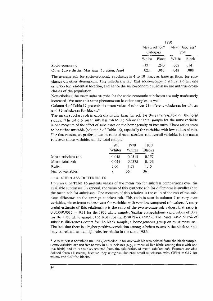
Socio-economic Other (Live Births, Marriage Duration, Age)

1970 Mean roh of* Mean Subclass*

Category roh

White Black White Black

.121

.021 .240 .068

.055

.048 .141 .088

The average roh for socio-economic subclasses is 4 to 10 times as large as those for sub­classes on other dimensions. This reflects the fact that socio-economic status is often one criterion for residential location, and hence the socio-economic subclasses are not true cross­classes of the population. Nevertheless, the mean subclass rohs for the socio-economic subclasses are only moderately increased. We note this same phenomenon in other samples as well. Column 4 of Table 17 presents the mean value of roh over 23 different subclasses for whites and 15 subclasses for blacks.* The mean subclass roh is generally higher than the roh for the same variable on the total sample. The ratio of mean subclass roh to the roh on the total sample for the same variable is one measure of the effect of subclasses on the homogeneity of measures. These ratios seem to be rather unstable (column 6 of Table 16), especially for variables with low values of roh. For that reason, we prefer to use the ratio of mean subclass roh over all variables to the mean roh over those variables on the total sample.

1960 1970 1970 Whites Whites Blacks

Mean subclass roh 0.048 0.0515 0.157 Mean total roh 0.024 0.0375 0.136 Ratio 2.00 1.37 1.15 No. of variables 9 36 36

3.6.4. SUBCLASS DIFFERENCES Column 6 of Table 16 presents values of the mean roh for subclass comparisons over the available subclasses. In general, the value of this synthetic roh for differences is smaller than the mean roh for subclasses. One measure of this relation is the ratio of the roh of the sub­class difference to the average subclass roh. This ratio is seen in column 7 to vary over variables; the extreme values occur for variables with very low computed roh values. A more useful estimate of this relationship is the ratio of the two average roh values; that ratio is 0.0055/0.0515 = 0.11 for the 1970 white sample. Similar computations yield ratios of 0.27 for the 1960 white sample, and 0.045 for the 1970 black sample. The lowest ratio of roh of subclass differences occurs for the black sample, a homogeneous group on most measures. The fact that there is a higher positive correlation among subclass means in the black sample may be related to the high rohs for blacks in the same PSUs.

* Any subclass for which the CV(x) exceeded .2 for any variable was deleted from the black sample. Some variables are not free to vary in all subclasses (e.g., number of live births among those with one live birth) and thus are also omitted from the calculation of mean subclass roh. Farmers are also deleted from all means, because they comprise clustered small subclasses, with CV(x) = 0.17 for whites and 0.50 for blacks.

56

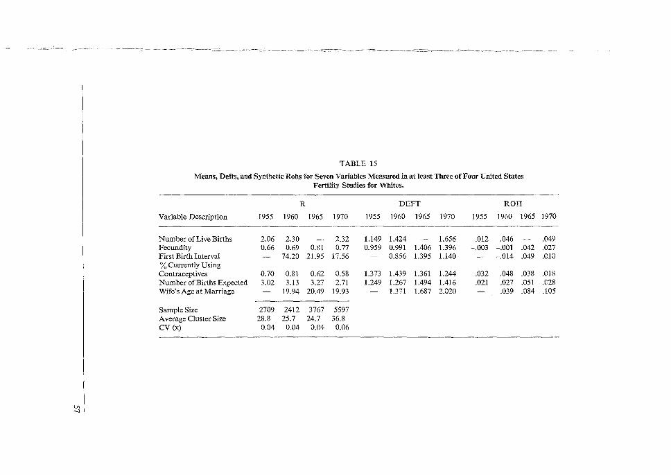
TABLE 15

Means, Defts, and Synthetic Rohs for Seven Variables Measured in at least Three of Four United States Fertility Studies for Whites.

R DEFT ROH

Variable Description 1955 1960 1965 1970 1955 1960 1965 1970 1955 1960 1965 1970

Number of Live Births 2.06 2.30 2.32 1.149 1.424 1.656 .012 .046 .049 Fecundity 0.66 0.69 0.81 0.77 0.959 0.991 1.406 1.396 -.003 -.001 .042 .027 First Birth Interval 74.20 21.95 17.56 0.856 1.395 1.140 -.014 .049 .010 % Currently Using Contraceptives 0.70 0.81 0.62 0.58 1.373 1.439 1.361 1.244 .032 .048 .038 .018 Number of Births Expected 3.02 3.13 3.27 2.71 1.249 1.267 1.494 1.416 .021 .027 .051 .028 Wife's Age at Marriage 19.94 20.49 19.93 1.371 1.687 2.020 .039 .084 .105

Sample Size 2709 2412 3767 5597 Average Cluster Size 28.8 25.7 24.7 36.8 CV (x) 0.04 0.04 0.04 0.06

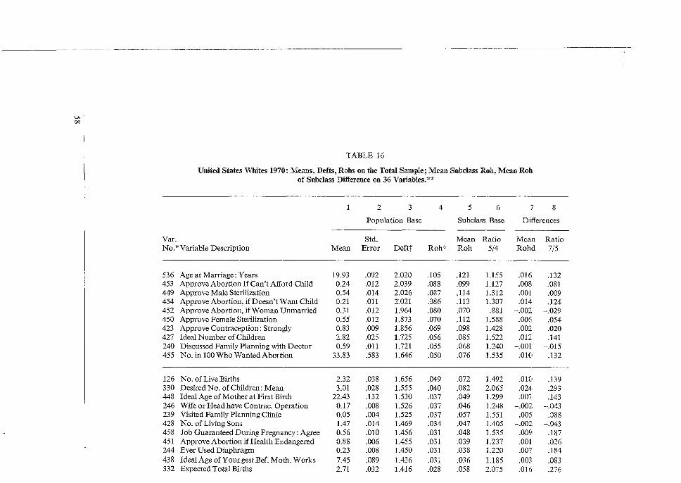
~I

TABLE 16

United States Whites 1970: Means, Defts, Rohs on the Total Sample; Mean Subclass Roh, Mean Roh of Subclass Difference on 36 Variables.**

2 3 4 5 6 .,

8 I

Population Base Subclass Base Differences

Var. Std. Mean Ratio Mean Ratio No.*Variable Description Mean Error Deftt Ro ht Roh 5/4 Rohd 7/5

536 Age at Marriage: Years 19.93 .092 2.020 .105 .121 1.155 .016 .132 453 Approve Abortion If Can't Afford Child 0.24 .012 2.039 .088 .099 1.127 .008 .081 449 Approve Male Sterilization 0.54 .014 2.026 .087 .114 1.312 .001 .009 454 Approve Abortion, if Doesn't Want Child 0.21 .011 2.021 .086 .113 1.307 .014 .124 452 Approve Abortion, if Woman Unmarried 0.31 .012 1.964 .080 .070 .881 -.002 -.029 450 Approve Female Sterilization 0.55 .012 1.873 .070 .112 1.588 .006 .054 423 Approve Contraception: Strongly 0.83 .009 1.856 .069 .098 1.428 .002 .020 427 Ideal Number of Children 2.82 .025 1.725 .056 .085 1.522 .012 .141 240 Discussed Family Planning with Doctor 0.59 .011 1.721 .055 .068 1.240 -.001 -.015 455 No. in lOOWho Wanted Abortion 33.83 .583 1.646 .050 .076 1.535 .010 .132

126 No. of Live Births 2.32 .038 1.656 .049 .072 1.492 .010 .139 330 Desired No. of Children: Mean 3.01 .028 1.555 .040 .082 2.065 .024 .293 448 Ideal Age of Mother at First Birth 22.43 .132 1.530 .037 .049 1.299 .007 .143 246 Wife or Head have Contrac. Operation 0.17 .008 1.526 .037 . 046 1.248 -.002 . -.043 239 Visited Family Planning Clinic 0.05 .004 1.525 .037 .057 1.551 .005 .088 428 No. of Living Som 1.47 .014 1.469 .034 .047 1.405 -.002 -.043 458 Job Guaranteed During Pregnancy: Agree 0.56 .010 1.456 .031 .048 1.535 .009 .187 451 Approve Abortion if Health Endangered 0.88 .006 1.455 .031 .039 1.237 .001 .026 244 Ever Used Diaphragm 0.23 .008 1.450 .031 .038 1.220 .007 .184 438 Ideal Age ofYotmgest Bef. Moth. Works 7.45 .089 1.436 .031 .036 1.185 .003 .083 332 Expected Total Births 2.71 .032 1.416 .028 .058 2.075 .016 .276

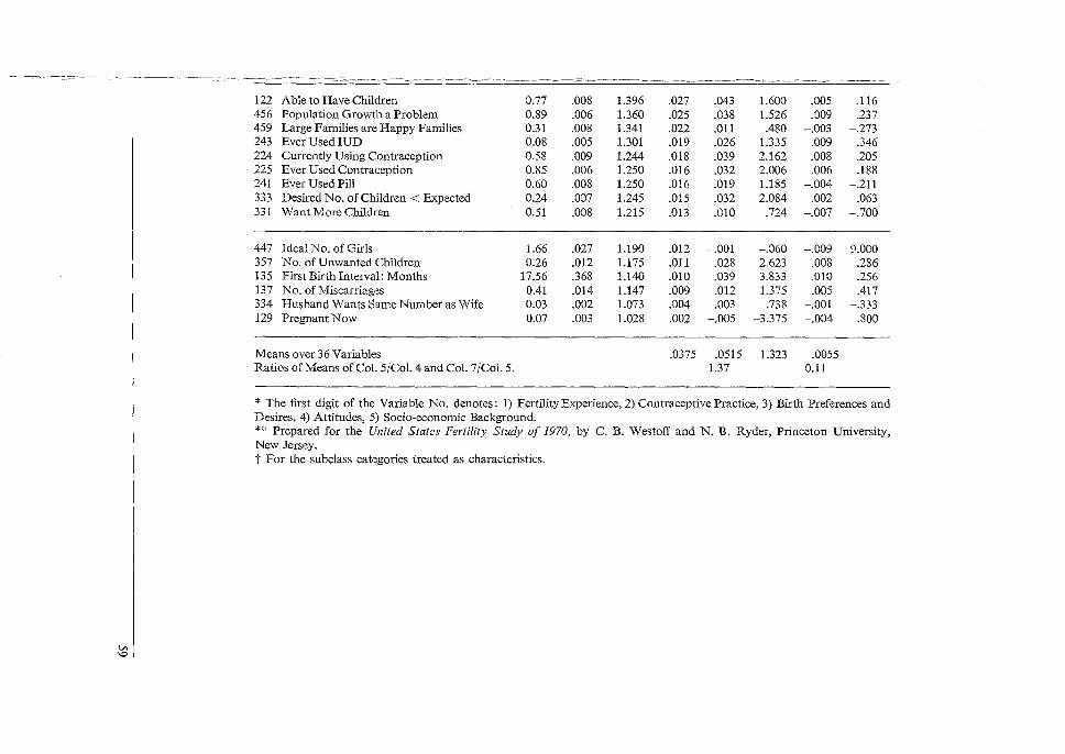
-- ~~c.~~--~- ,.~-----

---~------- ------~---~----------------~-~ ---~-~~---------~~-------~·-----"-~-~

122 Able to Have Children 0.77 .008 1.396 .027 .043 1.600 .005 .116 456 Population Growth a Problem 0.89 .006 1.360 .025 .038 1.526 .009 .237 459 Large Families are Happy Families 0.31 .008 1.341 .022 .011 .480 -.003 -.273 243 Ever Used IUD 0.08 .005 1.301 .019 .026 1.335 .009 .346 224 Currently Using Contraception 0.58 .009 1.244 .018 .039 2.162 .008 .205 225 Ever Used Contraception 0.85 .006 1.250 .016 .032 2.006 .006 .188 241 Ever Used Pill 0.60 .008 1.250 .016 .019 1.185 -.004 -.211 333 Desired No. of Children< Expected 0.24 .007 1.245 .015 .032 2.084 .002 .063 331 Want More Children 0.51 .008 1.215 .013 .010 .724 -.007 -.700

447 Ideal No. of Girls 1.66 .027 1.190 .012 -.001 -.060 -.009 9.000 357 No. of Unwanted Children 0.26 .012 1.175 .011 .028 2.623 .008 .286 135 First Birth Interval: Months 17.56 .368 1.140 .010 .039 3.833 .010 .256 137 No. ofMiscarriag1~s 0.41 .014 1.147 .009 .012 1.375 .005 .417 334 Husband Wants Same Number as Wife 0.03 .002 1.073 .004 .003 .738 -.001 -.333 129 Pregnant Now 0.07 .003 1.028 .002 -.005 -3.375 -.004 .800

Means over 36 Variable:s .0375 .0515 1.323 .0055 Ratios of Means of Col. 5/Col. 4 and Col. 7/Col. 5. 1.37 0.11

* The first digit of the Variable No. denotes: 1) Fertility Experience, 2) Contraceptive Practice, 3) Birth Preforences and Desires, 4) Attitudes, 5) Socio-economic Background. ** Prepared for the United States Fertility Study of 1970, by C. B. We5toff and N. B. Ryder, Princeton University, New Jersey. t For the subclass categories treated as characteristics.

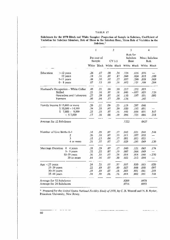
TABLE 17

Subclasses for the 1970 Black and White Samples: Proportion of Sample in Subclass, Coefficient of Variation for Subclass Members, Roh of Those in the Subclass Base, Mean Roh of Varhlbles in the

Subclass.*

2 3 4

Roh for Per cent of Subclass Mean Subclass

Sample CV (x) Base Roh

White Black White Black White Black White Black

Education > 12 years .26 .17 .08 .24 .124 .636 .076 12 years .18 .31 .07 .17 .049 .024 .035 .109

9-11 years .48 .35 .07 .17 .057 .290 .039 .069 0-- 8 years .07 .15 .09 .18 .052 .121 .108 .204

Husband's Occupation - White Collar .45 .21 .08 .20 .217 .252 .055 Skilled .23 .16 .07 .18 .043 -.057 .029 .126 Operatives and Labourers .27 .59 .07 .16 .110 .197 .051 .093 Farmers .05 .04 .17 .50 .136 .145

Family income$ 15,000 or more .20 .11 .09 .23 .119 .207 .046 $ 10,000 - 14,999 .38 .25 .07 .20 .020 .192 .051 $ 7,000- 9,999 .25 .33 .07 .16 .443 .058 .031 .167

< $ 7,000 .17 .31 .08 .19 .096 .725 .086 .218

Average for 12 Subclasses .1222 .0627

Number of Live Births 0--1 .34 .29 .07 .17 .042 .021 .048 .144 2 .26 .18 .07 .19 .011 .057 .035 3 .18 .15 .06 .17 .001 .013 .033 4 or more .21 .37 .07 .17 .029 .195 .049 .120

Marriage Duration 0- 4 years .28 .29 .07 .17 .040 .121 .065 .174 5- 9 years .22 .22 .07 .19 .007 .064 .049

10-19 years .36 .33 .07 .18 .014 .018 .048 -.270 20 or more .14 .16 .07 .20 .022 .212 .054

Age <25 years .24 .23 .07 .17 .037 .030 .053 .020 25-29 years .22 .19 .07 .19 .027 .048 .058 .097 30-34 years .19 .19 .07 .18 .003 .031 .041 .253 35-44 years .34 .39 .06 .16 .018 .002 .041 .168

Average for 12 Subclasses .0209 .0478 Average for 24 Subclasses .0716 .0553

* Prepared for the United States National Fertility Study of 1970, by C. B. Westoff and N. B. Ryder, Princeton University, New Jersey.

60

References

A detailed list of references is not given here; most of the concepts used can be found in the standard literature of survey sampling. Cochran, W. G. [1963], Sampling Techniques, 2nd ed., (New York and London, John Wiley and Sons). Hansen, M. H., Hurwitz, W. N., and Matlow, W. G. [1953], Sample Survey Methods and Theory,

(New York and London, John Wiley and Sons). Kish, L. [1965], Survey Sampling, (New York and London, John Wiley and Sons). Kish, L. and Frankel, M. R. [1974], 'Inference from complex samples', Journal of the Royal Statistical

Society (B), Vol. 36, pp. 1-37. Yates, F. [1960], Sampling Methods for Censuses and Surveys, 3rd ed., (London, Chas. Griffin and

Co).

61

WORLD FERTILITY SURVEY

OCCASIONAL PAPERS

1. Fertility and Related Surveys

2. The World Fertility Survey: Problems and Possibilities

World Fertility Survey Inventory: Major Fertility and Related Surveys 1960-73

3. Asia

4. Africa

5. Latin America

6. Europe, North America and Australia

7. The Study of Fertility and Fertility Change in Tropical Africa

8. Community-Level Data in Fertility Surveys

William G. Duncan

J. C. Caldwell

l Swnuel Baum '' al

John C. Caldwell

Ronald Freedman 9. Examples of Community-Level Questionnaires Ronald Freedman

10. A Selected Bibliography of Works on Fertility Gyorgy T. Acsadi 11. Economic Data for Fertility Analysi Deborah S. Freedman (with Eva Mueller)

12. Economic Modules for use in Fertility Surveys DeborahS.Freedman and Eva Mueller in Less Developed Countries

13. Ideal Family Size Helen Ware

14. Modernism David Goldberg

15. The Fiji Fertility Survey: M.A. Sahib et al A Critical Commentary

16. The Fiji Fertility Survey: M.A. Sahib et al A Critical Commentary-Appendices

17. Sampling Errors for Fertility Surveys L. Kish et al

18. The Dominican Republic Fertility Survey: N. Ramirez et al An Assessment

19. WFS Modules: Abortion · Factors other than WPS Central Staff Contraception Affecting Fertility · Family Planning . General Mortality

N.V. DRUKKERU TRIO •THE HAOUE •THE NETHERLANDS