1 THE HOUSEHOLD RESPONSE TO PERSISTENT NATURAL DISASTERS: EVIDENCE FROM BANGLADESH Azreen Karim* Victoria University of Wellington May, 2017 * JOB MARKET PAPER* Revised for World Development ABSTRACT Recent literatures examine the short-run effects of natural disasters on household welfare and health outcomes. However, less advancement has been observed in the use of self-reported data to capture the short-run disaster-development nexus in least developed countries’ with high climatic risks. This self-identification in the questionnaire could be advantageous to capture the disaster impacts on households’ more precisely when compared to index-based identifications based on geographical exposure. In this paper, we ask: ‘what are the impacts on household income, expenditure, asset and labor market outcomes of recurrent flooding in Bangladesh?’ We examine the short-run economic impacts of recurrent flooding on Bangladeshi households’ surveyed in year 2010. In 2010 Household Income and Expenditure Survey (HIES), households’ answered a set of questions on whether they were affected by flood and its likely impacts. We identify treatment (affected) groups using two measures of disaster risk exposure; the self-reported flood hazard data and historical rainfall data based flood risk index. The paper directly compares the impacts of climatic disaster (i.e. recurrent flooding) on economic development. We further examine these impacts by pooling the data for the years’ 2000, 2005 and 2010 and compare the results with our benchmark estimations. Overall, we find robust evidence of negative impacts on agricultural income and expenditure. Intriguingly, the self-reported treatment group experienced significant positive impacts on crop income. Key words: Economic Development; Natural Disasters; Persistent; Measures of disaster risk exposure; Agricultural income. *Corresponding email: [email protected]; [email protected]. I would like to gratefully thank the Editor-in-Chief and two anonymous reviewers’ for providing me insightful comments and constructive suggestions that helped me to improve the draft version of the paper. I am profoundly indebted to my supervisors, Professor Ilan Noy and Dr. Mohammed Khaled who were very generous with their time and knowledge to provide me guidance and thoughtful comments in the preliminary version of the paper. I am also grateful to Dr. Binayak Sen (Bangladesh Institute of Development Studies) and M.G. Mortaza (Asian Development Bank, BRM) for providing useful inputs in the data collection process. I thank the audiences of the 57 th Annual Conference of the New Zealand Association of Economists (NZAE); in particular Arthur Grimes, Mark Holmes, Andrea Menclova, and my Ph.D. thesis examiners’; Harold Cuffe, Asadul Islam and Professor David Fielding.

Welcome message from author
This document is posted to help you gain knowledge. Please leave a comment to let me know what you think about it! Share it to your friends and learn new things together.
Transcript

1
THE HOUSEHOLD RESPONSE TO PERSISTENT NATURAL DISASTERS: EVIDENCE FROM BANGLADESH
Azreen Karim* Victoria University of Wellington
May, 2017
* JOB MARKET PAPER*
Revised for World Development
ABSTRACT
Recent literatures examine the short-run effects of natural disasters on household welfare and health outcomes. However, less advancement has been observed in the use of self-reported data to capture the short-run disaster-development nexus in least developed countries’ with high climatic risks. This self-identification in the questionnaire could be advantageous to capture the disaster impacts on households’ more precisely when compared to index-based identifications based on geographical exposure. In this paper, we ask: ‘what are the impacts on household income, expenditure, asset and labor market outcomes of recurrent flooding in Bangladesh?’ We examine the short-run economic impacts of recurrent flooding on Bangladeshi households’ surveyed in year 2010. In 2010 Household Income and Expenditure Survey (HIES), households’ answered a set of questions on whether they were affected by flood and its likely impacts. We identify treatment (affected) groups using two measures of disaster risk exposure; the self-reported flood hazard data and historical rainfall data based flood risk index. The paper directly compares the impacts of climatic disaster (i.e. recurrent flooding) on economic development. We further examine these impacts by pooling the data for the years’ 2000, 2005 and 2010 and compare the results with our benchmark estimations. Overall, we find robust evidence of negative impacts on agricultural income and expenditure. Intriguingly, the self-reported treatment group experienced significant positive impacts on crop income.
Key words: Economic Development; Natural Disasters; Persistent; Measures of disaster risk exposure; Agricultural income. *Corresponding email: [email protected]; [email protected]. I would like to gratefully thank the Editor-in-Chief and two anonymous reviewers’ for providing me insightful comments and constructive suggestions that helped me to improve the draft version of the paper. I am profoundly indebted to my supervisors, Professor Ilan Noy and Dr. Mohammed Khaled who were very generous with their time and knowledge to provide me guidance and thoughtful comments in the preliminary version of the paper. I am also grateful to Dr. Binayak Sen (Bangladesh Institute of Development Studies) and M.G. Mortaza (Asian Development Bank, BRM) for providing useful inputs in the data collection process. I thank the audiences of the 57
th Annual Conference of the New Zealand Association of Economists (NZAE); in particular Arthur Grimes,
Mark Holmes, Andrea Menclova, and my Ph.D. thesis examiners’; Harold Cuffe, Asadul Islam and Professor David Fielding.
2
1. INTRODUCTION
Bangladesh has a long history with natural disasters due to its geography and its
location on the shores of the Bay of Bengal. Climate change models predict Bangladesh will
be warmer and wetter in the future.1 This changing climate induces flood risk associated
with the monsoon season each year (Gosling et al. 2011). It is now widely understood that
climate induced increasingly repeated risks threaten to undo decades of development
efforts and the costs would be mostly on developing countries impacting existing and future
development (OECD, 2003; McGuigan et al., 2002; Beg et al., 2002). Recent literatures
examine the short-run effects of natural disasters on household welfare and health
outcomes (Arouri et al., 2015; Lohmann and Lechtenfeld, 2015; Silbert and Pilar Useche,
2012; Rodriguez-Oreggia et al. 2013, Lopez-Calva and Juarez, 2009). However, less
advancement has been observed in the use of self-reported data to capture the short-run
disaster-development nexus in least developed countries with high climatic risks.2 In this
paper, we ask: ‘what are the impacts on household income, expenditure, asset and labor
market outcomes of recurrent flooding in Bangladesh?’
We examine the short-run economic impacts of recurrent flooding on Bangladeshi
households’ surveyed in year 2010. In 2010 Household Income and Expenditure Survey
(HIES), households answered a set of questions’ on whether they were affected by flood and
its likely impacts. This self-identification in the questionnaire could be advantageous to
capture the disaster impacts on households’ more precisely when compared to index-based
identifications based on geographical exposure. However, literatures have identified
shortcomings in self-reporting and various determinants of flood risk perception.3
Therefore, this paper contributes the following in the ‘disaster-development’ literature:
first, it identifies treatment (affected) groups using two measures of disaster risk exposure -
the self-reported flood hazard data and historical rainfall data based flood risk index;
second, it directly compares the impacts of climate disaster (i.e. recurrent flooding) on four
1 See Bandyopadhyay and Skoufias (2015).
2 Poapongsakorn and Meethom (2013) looked at the household welfare impacts of 2011 floods in Thailand (an
upper-middle income country by World Bank definition) and Noy and Patel (2014) further extended this to look at spill over effects. 3 Limitations of self-reported data have been detailed in Section 3(a).

3
development dimensions i.e. income, expenditure, asset and on labor market outcomes.
Our novelty in this paper is the identification of flood treatment households’ using self-
reported flood hazard data and historical rainfall-based flood risk index. The development
responses of the climatic disasters may therefore depend on the novel approach i.e.
accuracy in identifying the treatment groups using self- and non-self-reported data. In this
paper, we show that there is inconsistency between self- and non-self-reported information
based estimates with literature outcomes questioning the designation of survey questions
(related to natural shocks) and their usefulness to capture development impacts.
The paper is designed as follows: Section 2 describes the theoretical framework
between social vulnerability and community resilience. Section 3 reviews the empirical
evidences highlighting recent insights to explore the nexus between climatic disasters and
economic development in both developed and developing countries. Section 4 portrays our
identification strategy while Section 5 describes the data, provides detailed breakdown of
our methodological framework, identifies the key variables and justifies the choice of the
covariates with added descriptive statistics. In Section 6, we present and analyse the
estimation results comparing with previous literatures along with robustness checks in
Section 7. Finally, in Section 8 we conclude with relevant policy implications and also some
insight for further advancements.
2. SOCIAL VULNERABILITY AND COMMUNITY RESILIENCE: THEORETICAL FRAMEWORK
[FIGURE 1 HERE]
Figure 1 displays the conventional way to consider disaster risk as a function of the following
factors:
Risk/Disaster Risk = f (Hazard, Exposure, Vulnerability)
where a country’s pre-determined geo-physical and climatic characteristics are part of its
hazard profile compared to exposure which is largely driven by poverty forcing people to
live in more exposed and unsafe conditions (e.g. living in flood plains).4 Poverty is both a
driver and consequence of disaster risk particularly in countries with weak risk governance
4 See Karim and Noy (2016a).

4
(Wisner et al. 2004). Vulnerability in the above functional form depicts disaster risk not only
depends on the severity of hazards or exposure of urban living and human assets but also
the exposed population’s capacities to withstand and reduce the socio-economic impacts of
hazards.5 Therefore, disaster risk can be viewed as the intersection of hazard, exposure, and
vulnerability. Since resilience has often been defined as the flip-side of vulnerability6, there
seems to be a clear connection between disaster risk reduction efforts and enhancement of
community resilience as occurrence and severity of natural hazards is uncontrollable.
However, vulnerability is multi-dimensional and dynamic; hence it demands inter-
disciplinary approaches to understand both the physical and socio-economic aspects.
Literatures have attempted to put forth conceptual frameworks in various contexts and
identify global and community-level indicators to quantify vulnerability. Among them; the
Hazard-of-Place Model of Vulnerability (Cutter et al. 2003), the Pressure and Release Model
(Blaikie et al. 1994:23), the Social Vulnerability Model (Dwyer et al. 2004:5) and the
framework to approach social vulnerability (Parker et al. 2009; Tapsell et al. 2010) could be
particularly mentioned. In a study on community resilience to coastal hazards in the Lower
Mississippi River Basin (LMRB) region in South-eastern Louisiana, the Resilience Inference
Measurement (RIM) Model has been applied to assess the resilience of higher- and lower-
resilient communities (Cai et al., 2016). Interestingly, the authors’ identified the location of
the lower-resilient communities to be along the coastline and in lower elevation area (in the
context of developed country here) that has also been argued in the context of developing
countries’ (e.g. Karim and Noy, 2016a). Our aim in this paper is to understand this
relationship among hazard, vulnerability and exposure and look at the impacts of climate-
induced disaster risks (e.g. flood hazards) on various socio-economic dimensions (i.e.
income, consumption, asset and labor market outcomes).
5
See Noy and du Pont IV (2016).
6 See Crichton (1999) and Wilson (2012). However, Cutter et al. (2014) found evidences that inherent resilience
is not the opposite of social vulnerability using the Baseline Resilience Indicators for Communities (BRIC) metric.

5
3. CLIMATE DISASTERS AND DEVELOPMENT: EMPIRICAL EVIDENCES
The last few years have seen a new wave of empirical research on the consequences
of changes in precipitation patterns, temperature and other climatic variables on economic
development and household welfare. Climate-related natural disasters are expected to rise
as the earth is getting warmer with prospect of significant negative economic growth mostly
affecting the poor countries (Felbermayr and Gröschl, 2014; Acevedo, 2014). Vulnerable
economies for example, the Pacific islands could expect a growth drop by 0.7 percentage
points for damages equivalent to 1 percent of GDP in the year of the disaster (Cabezon et
al., 2015). On the causality between catastrophic events and long-run economic growth
using 6,700 cyclones, Hsiang and Jina (2014) find robust evidence that national incomes
decline compared to pre-disaster trends and the recovery do not happen for twenty years
for both poor and rich countries. This finding contrasts with the earlier work of Noy (2009)
and Fomby, Ikeda and Loayza (2009)7 to some extent and carry profound implications as
climate change induced repeated disasters could lead to accumulation of income losses over
time. Therefore, climate disasters have become a development concern with likelihood of
rolling back years of development gains and exacerbate inequality.
Climate resilience has become integral in the post-2015 development framework
and recent cross-country ‘micro’ literatures explore the channels through which climate
disasters impacted poverty.8 Recent studies on rural Vietnam looked at the impacts on
climate disasters such as floods, storms and droughts on household resilience, welfare and
health outcomes (Arouri, Nguyen and Youssef, 2015; Lohmann and Lechtenfeld, 2015; Bui et
al. 2014). Arouri et al. (2015) pointed out that micro-credit access, internal remittance and
social allowances could strengthen household resilience to natural disasters. However, high
resilience might not necessarily reflect low vulnerability as evident in a study conducted on
tropical coastal communities in Bangladesh (Akter and Mallick, 2013). Moreover, another
study on the Pacific island of Samoa by Le De, Gaillard and Friesen (2015) suggests that
differential access to remittances could increase both inequality and vulnerability.
Bandyopadhyay and Skoufias (2015) show that climate induced rainfall variability influence
7 These studies focus on the short-run effects of natural disasters.
8 Karim and Noy (2016a) provide a qualitative survey of the empirical literature on poverty and natural
disasters.

6
employment choices impacting lower consumption in flood-prone sub-districts in rural
Bangladesh. Agricultural specialization based occupational choices are also found to be
negatively affected with high variations in rainfall in the Indian context (Skoufias et al.
2017). Assessing relationship between household heterogeneity and vulnerability to
consumption patterns to covariate shocks as floods and droughts, Kurosaki (2015) identified
landownership to be a critical factor to cope with floods in Pakistan. A recent study on the
Indian state of Tamil Nadu by Balasubramanian (2015) estimates the impact of climate
variables (i.e. reduction in ground water availability at higher temperature than a threshold
of 34.310 C) on agricultural income impacting small land owners to get low returns to
agriculture. In one particular examination on occurrence and frequency of typhoons and/or
floods in Pasay City, Metro Manila by Israel and Briones (2014) reveals significant and
negative effects on household per capita income.
This literature also explored vulnerability to natural disasters in the context of
developed countries; for example, the case of hurricane Katrina in the US city of New
Orleans. Evidences suggest that the pre-existing socio-economic conditions and racial
inequality in New Orleans played a crucial role in exacerbating damages due to Hurricane
Katrina in addition to the failure of flood protection infrastructure and disaster anticipation
combined with poor responses management (Masozera et al.2007; Cutter et al. 2006; Levitt
and Whitaker, 2009). A recent study by Martin (2015) used a grounded theory approach to
develop the Social Determinants of Vulnerability Framework and applied on the US city of
Boston. The author found that those living with low-to-no income are at the highest risk for
negative post-incident outcomes. Bergstrand et al. (2015) adds to this social vulnerability-
community resilience to hazards literature by measuring these indices in counties across the
United States and find a correlation between high levels of vulnerability and low levels of
resilience (indicating that the most vulnerable counties also tend to be the least resilient).
The authors further identified that the Northern parts of the United States, particularly the
Midwest and northeast, were more resilient and less vulnerable than the South and West.
This finding has also been confirmed by Cutter et al. (2014) using an alternative resilience
metric.
This growing ‘Climate-Development’ literature further explores empirical patterns in
risk, shocks and risk management by using shock modules in questionnaire-based surveys to
7
complement existing risk management tools. This usage of self-reported information on
natural shocks motivated researchers to develop different dimension of identification
strategies and compare impact findings using econometric models. Two recent studies by
Noy and Patel (2014) and Poapongsakorn and Meethom (2013) investigate household
welfare and spill over effects of the 2011 Thailand flood identifying self-reported affected
(treatment) group in a difference-in-difference modelling framework. Nevertheless,
evidences suggest careful use of self-reported data in identifying the true impacts which is
also one of the highlights in this paper.9
(a) Limitations of Self-reported data
Recent studies have identified various limitations of reported flood risk and showed
that perceived flood exposure could be different from actual risk. In a study conducted in
Bray, Dublin city; O’Neill et al. (2016) finds that distance to the perceived flood zone
(perceived flood exposure) is a crucial factor in determining both cognitive and affective
components of flood-risk perception. Another recent study by Trumbo et al. (2016)
develops an interesting measure of risk perception (in the context of hurricanes) to
understand how people make decisions when facing an evacuation order. This literature
found to validate previous works and justifies its approach to other contexts within natural
hazards, and elsewhere. Self-reporting in terms of being affected could be subjective and
might bring biased results due to sorting or selective reporting.10 Self-reported data could
not only be a subject of recall error, but also to other forms of cognitive bias like reference
dependence (Guiteras, Jina and Mobarak, 2015).
4. IDENTIFICATION STRATEGY
Our objective in this paper is to analyse the short-run impacts of recurrent flooding
on household income, expenditure, asset and labor market outcomes through identification
of treatment (affected) groups using both self- and non-self-reported data (historical rainfall
9 See Guiteras, Jina, and Mobarak (2015) and Heltberg, Oviedo and Talukdar (2015).
10 See Heltberg, Oviedo and Talukdar (2015) for a discussion on how survey modules falls short of expectations
in several ways.

8
data based flood risk index). We use the term ‘persistent natural disasters’ to refer to
repeated natural disasters (e.g. flood) that occurs almost every year and possess increase
risks of occurrence due to rainfall variability.11 Our estimation strategy identifies affected
households’ using two different measures of disaster risk exposure (i.e. flood hazard) and
directly compares the impacts on various socio-economic outcomes. Our primary focus is
the year 2010 as shock module was introduced in the 2010 Household Income and
Expenditure Survey (HIES) with questionnaire related to natural disasters and no new
surveys have been conducted at the national level since then.12 The module on shocks and
coping responses was first introduced in HIES 2010 to identify households affected by
various idiosyncratic and covariate shocks. As our focus in this paper is on covariate shocks
i.e. flood, we identify households who have self-reported to be affected by floods only in
2010 survey. The earlier surveys – 2000 and 2005 did not have any shock module and hence
identification of self-reported affected groups was not possible. However, Bangladesh as a
disaster-prone country, disasters particularly flood is a repeated phenomenon every year.
Here, we took flood as persistent natural disaster due to its repeated occurrence every year
mostly during the monsoon period (May-October). Due to limitations of the self-reported
data (as evident in literatures), we identify two ‘treatment’ groups – treatment group A and
treatment group B to compare the impacts using two different measures of disaster risk
exposure.
The first treatment group i.e. treatment group A is identified through the self-
reported information using the shock module in year 2010. From 2010 survey, the
treatment group are the respondents who have said ‘Yes’ as being affected by flood hazard
only. In 2010, the comparison groups are those households who have responded ‘No’ to
being affected by flood hazard only. To identify our second treatment group i.e. treatment
group B, we use a rainfall-based flood risk probability index using historical rainfall dataset13
from the Bangladesh Meteorological Department (BMD) to identify upazilas/thanas14 (in
particular, the survey areas) which are affected by more than average rainfall over a long
11
See Bandyopadhyay and Skoufias (2015) and Gosling et al. (2011). 12
The decision process of 2015 survey is currently underway according to the information provided by the current Project Director of HIES. 13
Guiteras et al. (2015) use satellite data for rainfall, but find that this data is poorly correlated with actual flooding. 14
Sub-districts are named as ‘Upazilas/Thanas’ in Bangladesh.

9
period (1948-2012).15 The rule of thumb is the survey areas (i.e. upazilas/thanas) which have
experienced more than average rainfall compared to the benchmark of average rainfall of
64 years in the corresponding weather station in year 2010 only, the surveyed households’
in those upazilas falls under treatment group B. The comparison (not affected) group here
are those households’ who resided in survey areas that did not experience excessive rainfall
compared to the average rainfall of 64 years in the corresponding weather station in year
2010 only. The advantages of using different flood risk measure in comparable contexts are
twofold. First, it justifies homogeneous circumstances among affected households’ in terms
of a common natural shock i.e. flood. Second, we can directly compare the development
impacts on two different treatment groups and the differences could refer to discrepancies
in capturing the true impacts using shock module. Also, it fits well with the distinction
between covariate and idiosyncratic shocks. Households’ located in the areas with rainfall
shocks may not report that they are affected by floods or droughts e.g. if they are not
engaged in agriculture. Richer or more educated households may be able to smooth
consumption and in this case might not report being affected by rainfall shocks.16 It is also
possible that individuals with higher level of education over-report their preparedness
behavior in order to present themselves in a positive way following socially accepted
standards (Hoffmann and Muttarak, 2017).
[FIGURE 2 HERE]
Figure 2 represents the map showing the upzailas/thanas (i.e. sub-districts) in which
the two treatment groups had been located. The red symbol exhibits the self-reported
treatment areas (i.e. treatment group A) whereas the blue symbol locates the rainfall-based
treatment areas (i.e. treatment group B). There are some upazilas which are found similar in
terms of treatment (for both groups – A and B) and have been identified using the box
structure in Fig. 2.
15
A breakdown of the index construction has been provided in the Appendix. See Karim and Noy (2015) for more details. 16 We thank an anonymous reviewer for pointing out this interesting insight in our analysis.

10
5. DATA AND METHODOLOGY
(a) Data description
We use the 2010 Household Income and Expenditure Survey (HIES) of the
Bangladesh economy in our main analysis. The HIES is the nationally representative dataset
conducted by the Bangladesh Bureau of Statistics (BBS) (in affiliation with the Ministry of
Planning, Government of Bangladesh and technical and financial assistance from the World
Bank) that records information regarding income, expenditure, consumption, education,
health, employment and labor market, assets, measures of standard of living and poverty
situation for different income brackets in urban and rural areas. The BBS conducts this
survey every five (5) years. The latest HIES conducted in 2010 added four (4) additional
modules in which one refers to ‘Shocks and Coping’ (Section 6B) in the questionnaire. The
BBS HIES is a repeated cross-section dataset with randomly selected households in
designated primary sampling units (PSUs). Therefore, the strength of the dataset is large
sample size covering a broad range of households’. However, limitations are there in
capturing the impacts over time. We further utilize HIES data spanning over a time period of
10 years consisting of years’ 2000, 2005 and 2010 to check robustness of our main results.
The number of households’ in year 2000 is 7,440 with 10,080 and 12,240 in year 2005 and in
year 2010 respectively. We also use the Bangladesh Meteorological Department (BMD)
rainfall dataset from 1948-2012 (i.e. 64 years) for 35 weather stations across the country to
identify flood-affected treatment group in respective survey years under consideration.
(b) Methodological framework
Our main aim here is to examine the short-run economic impacts of recurrent
flooding on households’ socio-economic outcomes i.e. income, consumption, asset and on
labor market outcomes. We start by examining the most parsimonious specification:
𝑦𝑖j = α + 𝛽1 A𝑖j + 𝛽2 B𝑖j + 𝛽3 C𝑖j+ 𝛾 (𝑋𝑖j) + u𝑖j (1)

11
Where 𝑦𝑖j is the outcome variable for household (i) in sub-district (j) (i.e. income,
expenditure, asset and labor market outcomes), 𝛽1 represents the coefficient for treatment
group A (self-reported flood impacts only), 𝛽2 represents the coefficient for treatment
group B (flood-risk index based shocks only), 𝛽3 represents the coefficient for both self-
reported disaster (flood) impact and index-based identifications (C), 𝑋𝑖j denotes the control
variables indicating households’ socio-economic characteristics and infrastructural features,
and u𝑖j indicate the error term. We use robust standard errors for our hypothesis tests. The
distinction between treatment group A (self-reported) and treatment group B (flood-risk
index based) will allow us to directly compare the differences in terms of impacts using
these two different measures of disaster risk exposure on household welfare. The constant
term, α in our benchmark model will define the impacts on the comparison groups i.e.
households’ who are not affected by repeated flood hazards.
To further investigate whether household-level characteristics (e.g. rural,
landownership and more education) has impacts on disaster-risk identifications, we further
estimate the following equation:
𝑦𝑖j = α + 𝛽1 A𝑖j + 𝛽2 B𝑖j + 𝛽3 C𝑖j + 𝛾1 (𝑋𝑖j1) + 𝛾2 (𝑋𝑖j
2) + 𝛿1 (A𝑖j. 𝑋𝑖j2) + 𝛿2 (B𝑖j. 𝑋𝑖j
2) + 𝛿3 (C𝑖j. 𝑋𝑖j2)
+u𝑖j (2)
The coefficients of the interaction among the treatment groups – A, B, C and the household-
level characteristics i.e. rural, landownership and formal education (𝛿1, 𝛿2 and 𝛿3) will define
the effect of these characteristics on the magnitude of the impacts on the outcome
variables.
(c) Outcome variables and choice of the control variables
Appendix tables 1 and 2 show the lists of key outcome and the control variables
(continuous and categorical) and their descriptive statistics for two different sets of
treatment and control groups. Our outcome variables of interest include four sets of
development indicators. They are: income (income by category), expenditure
12
(expenditure/consumption by category), asset types and labor market outcomes. Income
and expenditure are divided into various sub-groups with statistics shown in per capita
household measures. Asset and labor market outcomes are also sub-divided into various
categories (also described in appendix tables 1 and 2). The continuous (monetary) variables
in each category are inflation-adjusted using consumer price index (CPI) data from the
Bangladesh Bank17 to allow for comparisons across different years.
Alleviating poverty is a fundamental challenge for Bangladesh with the majority of
the extreme poor living in rural areas with considerable flood risk bringing annual
agricultural and losses to livelihoods (JBIC, 2007; Fadeeva, 2014; Ferdousi and Dehai, 2014).
Hence, we control for ‘rural’ that takes the value 1 if the household resides in a rural area
and 0 if otherwise reported. The male member as household head is generally considered as
‘bread earner’ and a good amount of literature also highlighted the positive association
between female-headed households and poverty especially in developing countries (Mallick
and Rafi, 2010; Aritomi et al., 2008; Buvinic and Rao Gupta, 1997). Female-headed
households are particularly vulnerable to climate variability as well (Flato et al. 2017).
Therefore, a dummy variable has been created indicating 1 if the household head is male
and 0, if reported otherwise. Household characteristics such as age structure and number of
dependents are critical to analyse poverty status and one might expect larger number of
dependents leads to greater poverty (Kotikula et al., 2010; Haughton and Khandker, 2009;
Lanjouw and Ravallion, 1995). Education is also related with lower poverty (Kotikula et al.,
2010). Community-level characteristics such as access to sanitation and access to safe
drinking water are clearly associated with better health outcomes improving poverty status
(World Bank, 2014; Duflo et al., 2012) of households with access to electricity also showing a
positive trend in living standards (Kotikula et al., 2010). Therefore, three (3) binary variables
are created indicating 1 to imply access to these services, 0 otherwise. Ownership status of
households such as house and land has also been argued as important determinant of
poverty with owners of a dwelling place are found to be less vulnerable to flood risk (e.g.
Khatun, 2015; Tasneem and Shindaini, 2013; Gerstter et al., 2011; Meinzen-Dick, 2009;
17
Bangladesh Bank is the Central Bank of Bangladesh.

13
Rayhan, 2010). A description of these variables including summary statistics is also provided
in appendix tables 1 and 2.
(d) Descriptive statistics
We provide two sets of descriptive statistics for two different treatment and
comparison groups (treatment group A and treatment group B) in appendix tables 1 and 2
respectively. We present mean and standard deviation for various outcome categories and
control variables for both rainfall-based and self-reported treatment (affected) and
comparison (not affected) groups. Most of the income categories seem to be higher for the
comparison group compared to treatment for treatment group A (self-reported) with
exception in the ‘crop income’ category. The crop income per capita for treatment group A
is on average, almost 11 percent higher compared to the comparison group. The other
treatment group i.e. treatment group B (rainfall-based flood treatment households’) also do
not show too much variation in terms of mean income by categories. However, mean of the
‘other income’ turns out to be almost 10 percent lower for the comparison group compared
to treatment in treatment group B. The comparison group also have around 1.2 percent less
business income compared to treatment in contrary to most income categories in the non-
self-reported case. The expenditure categories also reveal interesting patterns in
agricultural expenditure (i.e. crop and non-crop), in particular. Non-crop expenditure in
treatment group A is about 4.5 percent higher with having a lesser variation in crop
expenditure (around 1.5 percent higher) compared to the comparison group. Agricultural
input also reveals a higher expenditure amount (i.e. approximately 2.5 percent) in treatment
compared to comparison group A. Interestingly, most of the expenditure categories in
comparison group B seems to be higher than treatment with exceptions in ‘non-crop’
expenditures (around 0.4 percent lower). Interesting contrast could also be portrayed in
educational and health expenditure categories for both treatment groups. Educational and
health expenditures are found to be less in comparison group B with exceptions in
comparison group A (in health expenditures) compared to their respective treatment groups
– B and A. However, on average, the educational and health expenditure are found to be
higher in self-reported treatment group (A) compared to the non-self-reported one (B). It is

14
here to note that, the proportion of household members getting access to formal education
exhibits almost similar pattern in both treatment and comparison groups - A and B. Parallel
trends could also be observed in terms of total change in agricultural and other business
asset categories between both treatment and comparison groups with marginal variation
(approximately 2.2 percent higher) observed in treatment in rainfall-based identifications.
Observable differences could also be seen in labor market outcomes between both
treatment and comparison groups. Daily wages are found to be somewhat higher (almost
0.7 percent) in treatment group B whereas households’ been identified in treatment group
A seems to earn more salaried wages (around 2 percent higher) compared to their
respective comparison groups – B and A. Intriguingly, the rainfall-based treatment
households (B) are found to earn more daily wages compared to more salaried wages
earned by the self-reported treatment (A) cases. There are interesting parallel trends in the
mean results of the control variables (independent variables) between the two treatment
groups. More self-reported households are found to reside in the rural areas showing their
dependency in rain-fed agriculture.18 The rainfall-based flood treatment households’
(treatment group B) have more working adults i.e. fewer dependents (around 0.3 percent)
compared to the self-reported identifications. However, the self-reported flood treatment
group owns more land (around 11 percent) and houses (almost 6 percent higher) compared
to the non-self-reported ones. Community characteristics such as access to sanitation, safe
drinking water and electricity also show parallel trends in their mean outcomes in both
treatment groups – A and B.
6. ESTIMATION RESULTS
We start by estimating our benchmark model (as specified in equation 1) with
treatment groups been identified using two measures of disaster risk exposure: self-
reported data (treatment group A) and historical rainfall-based flood risk index (treatment
group B). We estimate our model on development dimensions such as income, expenditure,
assets, and labor market outcomes. We therefore, compare our results for each category (in
18
See Haile (2005).
15
terms of aggregate and disaggregated outcome measures) with previous literatures and
extend our analysis by estimating our model specified in equation (2).
(a) Income
[TABLE 1 HERE]
Table 1 reports the impacts of recurrent-flooding on different income categories i.e.
crop, non-crop, business and other income for self-reported treatment group (A) and
rainfall-based flood affected treatment group (B). We find both treatment (affected)
households’ experience negative impacts on total income being consistent with previous
disaster literatures (e.g. Asiimwe and Mpuga, 2007; Thomas et al., 2010; De La Fuente,
2010). Our results indicate that total income reduces by almost 1.1 percent more (estimated
to be approximately BDT 11,665) for treatment group B compared to the mean.19 A decline
in crop income is significantly higher for treatment group B (by around BDT 3,456) whereas
both treatment group (C) observe comparatively greater reduction in non-crop income (by
approx. BDT 23,601) being consistent with evidences that show decline in agricultural
income due to rainfall shocks (e.g. Skoufias et al., 2012; Baez and Mason, 2008; UNISDR,
2012). We do not observe any significant negative impacts on business income (non-
agricultural enterprise) and other income in both treatment cases. These results could also
be justified by previous works done by Attzs (2008) and Patnaik and Narayanan (2010).
The rainfall-based affected group (treatment group B) experienced a fall in both crop
and non-crop income (although coefficient of crop income is significant). Although the self-
reported affected group (A) observed a fall in total income, there has been a significant
increase in crop income. However, crop income decreases by almost BDT 3,765 for both
treatment groups (C). The interesting thing to note here is that persistent flooding seems to
impact non-crop income in higher magnitude. Our results show that treatment group B
(rainfall-based) experienced a drop of almost BDT 12,566 more in non-crop income
compared to the treatment group A (self-reported). The other two categories of income we
analyse are business and other incomes which are more indirectly affected by flood hazards.
Business and other income are found to decrease (not significant) for the self-reported
19
1 US Dollar = 77.88 Bangladeshi Taka (BDT).

16
affected households’. However, in both of these categories, we observe positive coefficients
for affected households’ who had been identified through rainfall-based identifications.
We extend our analysis on households’ agricultural income (as assumed to have
direct impact through repeated flooding) by further investigating their relationship with
rural (defining reliance on agriculture), formal education and ownership of land.20
Agricultural income (crop and non-crop) are found to drop significantly for rainfall-based
affected households (B). Crop income is also found to decrease in higher magnitude in both
self and non-self-reported cases (but not significant). The interesting thing to note here is
that, crop income had increased quite significantly (around 5.6 percent more) compared to
the mean for treatment group A impacting on total income as well.
(b) Consumption / Expenditure
[TABLE 2 HERE]
We report impact estimates of various expenditure categories i.e. food, non-food,
crop, non-crop, agricultural input, education and health for non-self- and self-reported
treatment groups in table 2. Our results show a significant decline of around 1 percent
compared to the mean in total expenditure per capita (i.e. drop by approx. BDT 14,742) for
treatment group B (non-self-reported) being consistent with previous literatures (e.g.
Dercon, 2004; Auffret, 2003; Asiimwe and Mpuga, 2007; Jha, 2006; Shoji, 2010; Foltz et al.
2013). Interestingly, treatment group A (self-reported) reveal a positive impact on total
expenditure due to flooding. This result could also be justified by coping strategies, safety
net and micro-credit borrowing by households.21 Our focal categories i.e. crop and
agricultural input expenditures (as we assume these categories are directly related to
rainfall shocks and flood) show negative impacts for rainfall-based affected households’.
This evidence, however demonstrates significant decrease in agricultural input expenditure
in particular. Food and non-food expenditures are found to decrease in treatment groups –
A and B. However, although both categories show sign consistencies, non-food expenditures
are found to be statistically significant for treatment group B. This observation is found to
aggravate in further investigations associated with the interactions. This decrease in non-
20
Full tables are shown in the appendix and also in an online appendix. 21
See Khandker (2007); Demont (2013); Vicarelli (2010).

17
food spending is particularly of concern as it implies the possibility that disasters prevent
longer-term investments and therefore trap households in cycles of poorer education and
health outcomes and persistent poverty (Karim and Noy, 2016b). These evidences turn out
to be interesting when we extend our analysis by further investigating the relationship with
rural, formal education and landownership of households’.22 Interestingly, we find that crop
expenditure increases significantly for self-reported treatment group (A) (estimated BDT
21,798) whereas non-crop expenditure per capita significantly increases (estimated approx.
BDT 37,026) for both rainfall-based and self-reported treatment group (C).
The various categories of expenditure - food, non-food, crop, non-crop, agricultural
input, educational and health expenditure - could also be categorized based upon their time
horizons e.g. short- and medium to long-run impacts. Expenditure categories as food, non-
food and agricultural consumption indicate the short-term impacts whereas education and
health expenditures may lead to longer-term impacts. The treatment households (A only
and B only) experienced significant contrast in terms of the direct impacts (food and non-
food in estimated model with interactions).23 Positive estimates have been observed in
education and health spending for treatment groups A and B as well. However, the rainfall-
based affected households’ experienced a decrease in educational expenditure
(approximately by BDT 3,453) compared to sharp decrease by both flood treatment
households (C) (estimated approx. by BDT 17,473). Intriguingly, the total expenditure in the
self-reported treatment group (A) increases (although not significant) compared to a
significant decline for the non-self-reported group in our benchmark estimation.
(c) Asset
[TABLE 3 HERE]
Table 3 demonstrates the impacts of repeated-flooding on three asset categories:
changes in agricultural and other business asset, agricultural input asset value and consumer
durable asset value for both affected (treatment) groups. We do not observe much contrast
in these categories though. Both treatment group (C) experienced significant negative
impacts (estimated by BDT 178,097) on change in agricultural and other business asset quite
22
Full tables are shown in the appendix and also in an online appendix. 23
Estimated using equation (2).

18
consistent with previous evidences on asset categories (e.g. Mogues, 2011; Anttila-Hughes
and Hsiang, 2013). Intriguingly, the self-reported flood affected group (treatment group A)
observe significant positive impacts (estimated by BDT 90,455) in the category representing
agricultural input asset value. These evidences are particularly valid when we incorporate
interaction terms in our estimated model.24 Nevertheless, the self-reported flood treatment
households’ (A) experienced a decline on change in agricultural and other business assets
when the estimated model do not account for the interaction terms.
(d) Labor market
[TABLE 4 HERE]
We present impacts on labor market for both treatment group – A and B in table 4
and our results reveal contrasts in households’ experiences. Daily wages are not found to be
severely affected (positive impact) with statistical significance for rainfall-based flood
treatment households’ (estimated by BDT 146).25 This somewhat been justified in some
previous empirical researches (e.g. Shah and Steinberg, 2012; Banerjee, 2007).26 However,
real wages are found to decrease for flood affected (self-reported) households’ in both
estimations 1 and 2 (but in this case without statistical significance). Interestingly, salaried
wage seems 2.7 percent higher compared to the mean (estimated approx. BDT 2,969) in
treatment group A with 0.3 percent drop (compared to the mean) for treatment group B but
without statistical significance as well.27 This result is also partially found consistent with the
findings of Mueller and Quisumbing (2011). The other labor market outcomes are found to
significantly improve for flood-affected (rainfall-based) households’ when the estimated
model (eq. 2) interacted with rural, formal education and land ownership status.28 We also
observe a contrast in estimates of yearly benefits for treatment groups – A and B.
24
Full tables are shown in the appendix and also in an online appendix. 25
Estimated using equation (2). 26
Banerjee (2007) find that floods have positive implications for wages in the long run. Interestingly, Mueller and Osgood (2009) reveal that droughts have significant negative impacts on rural wages in the long run. We are quite agnostic on the general implications of natural disasters on wages due to limitations in this study. 27
Estimated using equation (1). 28
Full tables are shown in the appendix and also in an online appendix.

19
(e) Control variables
[TABLE 5 HERE]
We present the coefficients of the control variables for the main variables of interest
in table 5.29 The coefficients of the control variables do not vary substantially in terms of
sign and significance for treatment groups – A, B and C. Among the controls; male-headed
households, average age, and formal education seems to have a stronger positive
association (highly significant) with total income and total expenditure per capita in addition
to community characteristic such as access to sanitation. Ownership of land demonstrates a
stronger positive impact (highly significant) on per capita total expenditure. It is more likely
that the household heads possess control over ownership of land and house.30 However, the
number of dependents displays a stronger negative association with total expenditure as
evident in the literatures as well. We also anticipate similar reasoning as of previous
literatures for observing the control variables to be in expected directions for asset
categories and labor market outcomes. The directions of the control variables are also
found quite similar when the model has been estimated by incorporating the interaction
terms (eq.2).
(f) Interaction terms
[TABLE 6 HERE]
To further investigate whether household characteristics e.g. rural, formal education
and landownership status have impacted declines in the development dimensions; we
estimate our model (eq.2) by incorporating the interaction terms. Table 6 present only the
results of the interplay among the identified treatment groups – A, B and C with rural,
formal education and landownership status.31 Interestingly, when the interaction terms are
included in the model, they seem to increase both the main effects of the treatment groups
and the respective control variables. The interaction terms between self-reported flood
treatment households’ and education in total income and total expenditure per capita are
found to be negative and statistically significant. This could imply that more educated
29
Full tables are shown in the appendix and also in an online appendix. 30
See Zaman (1999). 31
Full tables are shown in the appendix and also in an online appendix.

20
households may be able to smooth consumption and in this case might not report being
affected by rainfall shocks. Alternatively, education has a positive influence on disaster
preparedness only for those who have not yet experienced a disaster in the past (Hoffmann
and Muttarak, 2017). Landownership seems to play a crucial role for the rainfall-based flood
treatment households’. The coefficients of the interaction terms for per capita total income
and expenditure between treatment group B and landownership are found to be positive
and statistically significant (not in higher magnitude) and are also consistent with previous
literatures (e.g. Kurosaki, 2015).
7. ROBUSTNESS CHECKS
As robustness checks, we further examine these impacts by pooling the data for the
years’ 2000, 2005 and 2010 and compare the results with our benchmark estimations. As
self-reported data were unavailable for years’ 2000 and 2005; we therefore, estimate
equations 1 and 2 through identifications of flood treatment households’ using rainfall-
based disaster risk measure only to check robustness of our main results.32 We also add year
fixed effects in our estimated models.33
In the income category, we observe significantly negative impacts on non-crop
income (drop by approx. BDT 8,497)34 due to persistent flood hazard. The interesting aspect
to note here is that agricultural income (in particular, non-crop income) is found to decline
more (additional drop by around BDT 9402) in our focal year 2010 for flood-treatment
households’ that are rainfall-based only. However, business income is found to increase
significantly when the estimated model interacted with rural, formal education and
landownership status (eq.2). Our findings also reveal a significant positive increase in other
income category with no interactions being consistent with our prior estimations.
We find consistency in the robust coefficients in total expenditure category
compared to our baseline model specifications. Flood treatment households’ experienced a
32
The full tables of the robustness check estimation results are shown in the appendix and also in an online appendix. 33 We estimate the following equation and extend by adding the interaction terms (as of eq.2) to check robustness
of our main results: 𝑦𝑖jt = αt + 𝛽2 B𝑖jt + 𝛾 (𝑋𝑖jt) + u𝑖jt 34
Estimated using equation (1) i.e. without interaction terms.

21
significant decline in total expenditure, in particular non-food and agricultural input
expenditure (eq.1). These impact evidences are found to exacerbate when food
expenditures are also observed to decrease significantly.35 The noticeable aspect here is
that findings reveal an additional decline in agricultural input expenditure (estimated
around BDT 4,606) significantly contributing to an excess decline in total expenditure (by
approx. BDT 10,225) for flood treatment households’ (rainfall-based). Non-food
expenditures also seems to contribute to this overall expenditure decline (an additional
drop by approx. BDT 4,238) and are found consistent with the benchmark estimation
results. Educational and health expenditures are also found to be consistent with our prior
estimations.
The impacts on agricultural input asset value display negative impacts on treatment
households’ (rainfall-based flood risk measure) that are found consistent with the
benchmark results. Interestingly, the impacts on changes in agricultural and other business
asset category exhibit positive coefficient (not significant) compared to a decline in prior
estimation results.36 The category on consumer durable asset value also illustrates
consistency in the estimated coefficients for flood treatment households’. The various
outcomes of the labor market do not seem to significantly vary with prior estimations as
well.
8. CONCLUSION
Our objective in this paper is to estimate the impacts of recurrent flooding on
income, expenditure, asset and labor market outcomes. We start with identification of the
treatment (affected) groups adopting two measures of disaster risk exposure i.e. using self-
reported flood hazard data and non-self-reported (historical rainfall-based flood risk index)
information in year 2010. We examine a parsimonious model to directly compare the short-
run impacts of climatic disaster (i.e. repeated flood hazard) on households’ socio-economic
outcomes. Our results suggest a decline in agricultural income (crop and non-crop) for both
35
This is evident when the estimated model interacted with landownership, rural and formal education of households’. 36
Estimated using eq. (2).

22
treatment group – A (self-reported) and B (rainfall-based). This significant decline in
agricultural income, being consistent with previous literatures reveals a clear message on
timely adoption of insurance in the context of increased climatic threat to achieve
sustainable poverty goals especially in agriculture-based economy like Bangladesh. As per
expenditure in concerned, we also observe a negative response to crop and agricultural
input expenditure in our focal categories (as we assume these categories are directly related
to rainfall shocks and flood) and are found consistent with our theoretical prior for rainfall-
based flood treatment households’. In particular, this evidence demonstrates a significant
decrease in agricultural input expenditure for treatment group B. A sharp decline in non-
food spending for these treatment households’ is also of policy concern as this suggests
decreased spending in health and education impacting longer-term investment.37
We extend our analysis by further interacting treatment groups’ with household
characteristics such as rural, formal education and ownership of land status. The interaction
terms seems to increase both the main effects of the treatment groups and the respective
control variables. Agricultural income (crop and non-crop) are found to drop significantly for
rainfall-based affected households’ (B). Interestingly, we find that crop expenditure
increases significantly for self-reported flood treatment households’ whereas non-crop
expenditure per capita significantly increases for households’ who have both self-reported
and been identified through geographical exposure (C). We further strengthen our results
pooling data from the earlier years’ i.e. 2000, 2005 and 2010 as robustness checks and
observe consistencies in most cases with our benchmark estimation results. We however,
only use the rainfall-based index measure in our robustness due to unavailability of self-
reported data in years’ 2000 and 2005.
The ‘disaster-development’ literature has made considerably less progress on the
use of shock modules to empirically estimate the impacts of natural disasters on
development outcomes. The recent addition of shock questionnaires in nationally
representative household income and expenditure surveys provides an ample scope to
identify the self-reported affected groups in repeated natural disasters. This self-
identification in the questionnaire could be advantageous to capture the disaster impacts on
households’ more precisely when compared to index-based identifications based on
37
See Karim and Noy (2016b) for a detailed analysis on this issue.

23
geographical exposure. However, literatures have identified shortcomings in self-reporting
and various determinants of flood risk perception. The dissimilarities in the results in terms
of the development impacts on flood treatment households’ using different measures of
disaster risk exposure might be due to the various shortcomings been identified in the
literatures. Moreover, questions’ based on ‘yes/no’ responses (i.e. close-ended) might not
be sufficient to identify the true development impacts. The selection of the respondents
(sample) in this particular set of questionnaire (shock questions on natural disasters) is also
questionable depending on criteria.38 There is an obvious need to employ both qualitative
and quantitative techniques to understand the degrees of experience in impact analysis.39
One possible solution is, of course, more respondents and data availability in addition to
incorporating degrees of actual hazard awareness, experience, and preparedness questions’
to identify the real affected group in repeated natural shocks. There is a need to thoroughly
analyse the inconsistencies in the robust research findings based on the shortcomings
identified in the literature. However, the evidence and the novel approach that we adopt in
this paper could justify future research in estimating welfare impacts of climate-induced
persistent natural events in developing countries.
REFERENCES
Acevedo, S. (2014). Debt, Growth and Natural Disasters A Caribbean Trilogy. IMF Working
paper no. WP/14/125.
Akter, S., Mallick, B. (2013). The poverty-vulnerability-resilience nexus: Evidence from
Bangladesh. Ecological Economics 96: 114–124.
Anttila-Hughes, JK and HM Solomon (2013). Destruction, Disinvestment, and Death:
Economic and Human Losses Following Environmental Disaster. Available at SSRN:
http://ssrn.com/ abstract=2220501 or http://dx.doi.org/10.2139/ssrn.2220501.
38
See Hawkes and Rowe (2008). 39
See Bird (2009).

24
Aritomi, T., A. Olgiati and M. Beatriz Orlando (2008). Female Headed Households and
Poverty in LAC: What are we measuring? Downloaded from:
http://paa2008.princeton.edu/papers/81458.
Arouri, M., Nguyen, C., & Youssef, A. B. (2015). Natural Disasters, Household Welfare, and
Resilience: Evidence from Rural Vietnam. World Development, 70, 59-77.
Asiimwe, JB and P Mpuga (2007). Implications of rainfall shocks for household income and
consumption in Uganda. AERC Research Paper 168, African Economic Research Consortium.
Attzs, M (2008). Natural disasters and remittances: Exploring the linkages between poverty,
gender and disaster vulnerability in Caribbean. SIDS No. 2008.61, Research paper/UNU-
WIDER.
Auffret, P (2003). High consumption volatility: The impact of natural disasters? World Bank
Policy Research working paper 2962, The World Bank.
Bangladesh Bank. Central Bank of Bangladesh. https://www.bb.org.bd/
Bangladesh Bureau of Statistics (BBS). Government of Bangladesh.
http://www.bbs.gov.bd/home.aspx.
Bangladesh Meteorological Department (BMD). Dhaka. www.bmd.gov.bd.
Bandyopadhyay, S and E Skoufias (2015). Rainfall variability, occupational choice, and
welfare in rural Bangladesh. Review of Economics of the Household, Vol. 13(3), pp. 1–46.
Baez, J and A Mason (2008). Dealing with climate change: Household risk management and
adaptation in Latin America. Available at SSRN 1320666.

25
Balasubramanian, R. (2015). Climate Sensitivity of Groundwater Systems Critical for
Agricultural Incomes in South India. SANDEE Working Papers, ISSN 1893-1891; WP 96–15.
Banerjee, L (2007). Effect of flood on agricultural wages in Bangladesh: An empirical
analysis. World Development, 35(11), pp. 1989–2009.
Beg, N., J. C. Morlot , O. Davidson , Y. Afrane-Okesse ,L. Tyani , F. Denton , Y. Sokona , J. P.
Thomas , Emilio Lèbre La Rovere , Jyoti K. Parikh , Kirit Parikh & A. Atiq Rahman (2002).
Linkages between climate change and sustainable development, Climate Policy, 2:2-3, 129-
144, DOI: 10.3763/cpol.2002.0216.
Bergstrand, K., Mayer, B., Brumback, B., & Zhang, Y. (2015). Assessing the relationship
between social vulnerability and community resilience to hazards. Social Indicators
Research, 122(2), 391-409.
Bird, D. K. (2009). The use of questionnaires for acquiring information on public perception
of natural hazards and risk mitigation–a review of current knowledge and practice. Natural
Hazards and Earth System Science, 9(4), 1307-1325.
Blaikie, P., T. Cannon, I. Davis, and B. Wisner (1994). At Risk London: Routledge.
Bui, A. T., Dungey, M., Nguyen, C. V., & Pham, T. P. (2014). The impact of natural disasters
on household income, expenditure, poverty and inequality: evidence from Vietnam. Applied
Economics, 46(15), 1751-1766.
Buvinic, M. & G.R. Gupta (1997). Female-Headed Households and Female-Maintained
Families: Are They Worth Targeting to Reduce Poverty in Developing Countries? Economic
Development and Cultural Change, Vol. 45, No. 2 (Jan., 1997), pp. 259-280.
Cabezon, E., Hunter, M. L., Tumbarello, M. P., Washimi, K., & Wu, M. Y. (2015). Enhancing
Macroeconomic Resilience to Natural Disasters and Climate Change in the Small States of
the Pacific. IMF Working paper no. WP/15/125.
26
Cai, H., Lam, N. S. N., Zou, L., Qiang, Y., & Li, K. (2016). Assessing Community Resilience to
Coastal Hazards in the Lower Mississippi River Basin. Water, 8(2), 46.
Crichton, D. (1999). The Risk Triangle, pp. 102-103 in Ingleton, J. (ed.), Natural Disaster
Management, Tudor Rose, London.
Cutter, S. L., B. J. Boruff and W. L. Shirley (2003). Social Vulnerability to Environmental
Hazards, Social Science Quarterly 84, no. 1: 242–61.
Cutter, S. L., Emrich, C. T., Mitchell, J. T., Boruff, B. J., Gall, M., Schmidtlein, M. C., ... &
Melton, G. (2006). The long road home: Race, class, and recovery from Hurricane Katrina,
Environment: Science and Policy for Sustainable Development, 48(2), 8-20.
Cutter, S.L., Ash, K.D. & Emrich, C.T., (2014). The geographies of community disaster
resilience. Global Environmental Change, 29, 65–77.
De la Fuente, A (2010). Natural disaster and poverty in Latin America: Welfare impacts and
social protection solutions. Well-Being and Social Policy, 6(1), 1–15.
Demont, T. (2013). Poverty, Access to Credit and Absorption of Weather Shocks: Evidence
from Indian Self-Help Groups. Downloaded from
http://www.greqam.fr/sites/default/files/_evenements/p198.pdf.
Dercon, S (2004). Growth and Shocks: Evidence from Rural Ethiopia. Journal of Development
Economics, 74(2), 309–329.
Duflo, E., Galiani, S., & Mobarak, M. (2012). Improving Access to Urban Services for the Poor:
Open Issues and a Framework for a Future Research Agenda. J-PAL Urban Services Review
Paper. Cambridge, MA: Abdul Latif Jameel Poverty Action Lab.

27
Dwyer, A.; C. Zoppou; O. Nielsen; S. Day; S. Roberts (2004). Quantifying Social Vulnerability:
A methodology for identifying those at risk to natural hazards. Geoscience Australia Record
2004/14.
Fadeeva, A. (2014). A comparative study of poverty in China, India, Bangladesh, and
Philippines. University of Southern California, Department of Sociology Working paper.
Downloaded from: https://dlc.dlib.indiana.edu/dlc/bitstream/handle/10535/9613/Fadeeva.
percent20A percent20comparative percent20study percent20of
percent20poverty.pdf?sequence=1&isAllowed=y.
Felbermayr, G., & Gröschl, J. (2014). Naturally negative: The growth effects of natural
disasters. Journal of Development Economics, 111, 92-106.
Ferdousi, S., & Dehai, W. (2014). Economic Growth, Poverty and Inequality Trend in
Bangladesh. Asian Journal of Social Sciences & Humanities Vol, 3, 1.
Flatø, M., Muttarak, R., & Pelser, A. (2017). Women, Weather, and Woes: The Triangular
Dynamics of Female-Headed Households, Economic Vulnerability, and Climate Variability in
South Africa. World Development, 90, 41-62.
https://doi.org/10.1016/j.worlddev.2016.08.015
Foltz, J, J Gars, M Özdogan, B Simane and B Zaitchik (2013). Weather and Welfare in
Ethiopia. In 2013 Annual Meeting, August 4–6, 2013, Washington DC, No. 150298,
Agricultural and Applied Economics Association.
Fomby, T., Ikeda, Y., & Loayza, N. V. (2013). The growth aftermath of natural disasters.
Journal of Applied Econometrics, 28(3), 412-434.
Gerstter, C., Kaphengst,T., Knoblauch,D. & Timeus, K. (2011). An Assessment of the Effects
of Land Ownership and Land Grab on Development–With a Particular Focus on Small
holdings and Rural Areas. European Parliament ad-hoc briefing EXPO/DEVE/2009/Lot 5/13.

28
Downloaded from:
http://www.ecologic.eu/sites/files/project/2013/lot5_13_land_grabbing_en.pdf.
Gosling, S. N., Dunn, R., Carrol, F., Christidis, N., Fullwood, J., Gusmao, D. D., ... & Warren, R.
(2011). Climate: Observations, projections and impacts: Bangladesh. Climate: Observations,
projections and impacts. Downloaded from:
http://eprints.nottingham.ac.uk/2040/6/Bangladesh.pdf.
Guiteras, R.P., A.S. Jina and A.M. Mobarak (2015). Satellites, Self-reports, and Submersion:
Exposure to Floods in Bangladesh . American Economic Review: Papers and Proceedings
105(5): 232-36.
Haile, M. (2005). Weather patterns, food security and humanitarian response in sub-
Saharan Africa. Philosophical Transactions of the Royal Society B: Biological Sciences,
360(1463), 2169-2182.
Haughton, Jonathan & Khandker, Shahidur R.(2009). Handbook on Poverty and Inequality.
The World Bank. Washington DC.
Hawkes, G. and Rowe, G. (2008). A characterisation of the methodology of qualitative
research on the nature of perceived risk: trends and omissions, J. Risk. Res., 11, 617–643.
Heltberg, R., Oviedo, A. M., & Talukdar, F. (2015). What do Household Surveys Really Tell Us
about Risk, Shocks, and Risk Management in the Developing World?. The Journal of
Development Studies, 51:3, 209-225. DOI: 10.1080/00220388.2014.959934
Hoffmann, R., & Muttarak, R. (2017). Learn from the past, prepare for the future: Impacts of
education and experience on disaster preparedness in the Philippines and Thailand. World
Development, 96, 32-51.

29
Hsiang, S. M., & Jina, A. S. (2014). The causal effect of environmental catastrophe on long-
run economic growth: evidence from 6,700 cyclones. National Bureau of Economic Research
Working Paper 20352. http://www.nber.org/papers/w20352.
IPCC (2014). Summary for policymakers. In: C.B. Field, et al., eds. Climate change 2014:
impacts, adaptation, and vulnerability. Part A: Global and sectoral aspects. Contribution of
Working Group II to the Fifth Assessment Report of the Intergovernmental Panel on Climate
Change [online]. Cambridge: Cambridge University Press, 1–32. Available from: http://ipcc-
wg2.gov/AR5/
Israel, D. C., & Briones, R. M. (2014). Disasters, Poverty, and Coping Strategies: The
Framework and Empirical Evidence from Micro/Household Data-Philippine Case. Philippine
Institute for Development Studies. Discussion Paper Series No. 2014-06.
Japan Bank for International Cooperation, JBIC (2007). Poverty Profile: People’s Republic of
Bangladesh. Downloaded from:
http://www.jica.go.jp/activities/issues/poverty/profile/pdf/bangladesh_e.pdf.
Jha, R (2006). Vulnerability and Natural Disasters in Fiji, Papua New Guinea, Vanuatu and
the Kyrgyz Republic. Available at http://dx.doi.org/10.2139/ssrn.882203.
Karim, A., & Noy, I. (2016a). Poverty and Natural Disasters–A Qualitative Survey of the
Empirical Literature. The Singapore Economic Review, 61(1), DOI:
http://dx.doi.org/10.1142/S0217590816400014.
Karim, A., & Noy, I. (2016b). Poverty and Natural Disasters: A Regression Meta-Analysis.
Review of Economics and Institutions, 7(2), 26.
Karim, Azreen and Noy, Ilan (2015). The (mis)allocation of Public Spending in a low income
country: Evidence from Disaster Risk Reduction spending in Bangladesh. School of Economics
and Finance Working Paper no. 4194, Victoria University of Wellington, New Zealand.

30
Khandker, SR (2007). Coping with flood: Role of institutions in Bangladesh. Agricultural
Economics, 36(2), 169–180.
Khandker, S. R., Bakht, Z., & Koolwal, G. B. (2009). The poverty impact of rural roads:
evidence from Bangladesh. Economic Development and Cultural Change, 57(4), 685-722.
Khatun, Razia (2015). The Impact of Micro-Level Determinants of Poverty in Bangladesh: A
Field Survey. International Journal of Research in Management & Business Studies, Vol. 2
Issue 2. Downloaded from: http://ijrmbs.com/vol2issue2/dr_razia1.pdf.
Kotikula, A., Narayan, A., & Zaman, H. (2010). To what extent are Bangladesh's recent gains
in poverty reduction different from the past? World Bank Policy Research Working Paper
Series, No. WPS5199.
Kurosaki, Takashi (2015). Vulnerability of household consumption to floods and droughts in
developing countries: evidence from Pakistan. Environment and Development Economics,
20, pp 209-235. DOI: 10.1017/S1355770X14000357.
L. Le De, J. C. Gaillard & W. Friesen (2015) Poverty and Disasters: Do Remittances Reproduce
Vulnerability? The Journal of Development Studies, 51:5, 538-553, DOI:
10.1080/00220388.2014.989995.
Lanjouw, P., & Ravallion, M. (1995). Poverty and household size. The Economic Journal,
1415-1434.
Levitt, J. I., & Whitaker, M. C. (2009). Truth crushed to earth will rise again Katrina and its
aftermath. In Hurricane Katrina: America's Unnatural Disaster (pp. 1-21). University of
Nebraska Press.
Lohmann, S., & Lechtenfeld, T. (2015). The Effect of Drought on Health Outcomes and
Health Expenditures in Rural Vietnam. World Development, 72, 432-448.

31
Lopez-Calva, L. F., & Ortiz-Juarez, E. (2009). Evidence and Policy Lessons on the Links
between Disaster Risk and Poverty in Latin America: Summary of Regional Studies, RPP LAC –
MDGs and Poverty – 10/2008, RBLAC-UNDP, New York. Downloaded from:
http://www.preventionweb.net/english/hyogo/gar/background-
papers/documents/Chap3/LAC-overview/LAC-Oveview.pdf.
Mallick, D., & Rafi, M. (2010). Are female-headed households more food insecure? Evidence
from Bangladesh. World Development, 38(4), 593-605.
Martin, S. A. (2015). A framework to understand the relationship between social factors that
reduce resilience in cities: Application to the City of Boston. International journal of disaster
risk reduction, 12, 53-80.
Masozera, M., Bailey, M., & Kerchner, C. (2007). Distribution of impacts of natural disasters
across income groups: A case study of New Orleans. Ecological Economics, 63(2), 299-306.
McGuigan, C., R. Reynolds & D. Wiedmer (2002). Poverty and Climate Change: Assessing
Impacts in Developing Countries and the Initiatives of the International Community. The
Overseas Development Institute. Downloaded from:
http://www.odi.org/sites/odi.org.uk/files/odi-assets/publications-opinion-files/3449.pdf.
Meinzen-Dick, Ruth S. (2009). Property Rights for Poverty Reduction? DESA Working Paper
No. 91. New York: United Nations Department of Economic and Social Affairs. Downloaded
from: http://www.un.org/esa/desa/papers/2009/wp91_2009.pdf.
Mogues, T (2011). Shocks and asset dynamics in Ethiopia. Economic Development and
Cultural Change, 60(1), 91–120.
Mueller, V. A., & Osgood, D. E. (2009). Long-term impacts of droughts on labor markets in
developing countries: evidence from Brazil. The Journal of Development Studies, 45(10),
1651-1662.

32
Mueller, V and A Quisumbing (2011). How resilient are labor markets to natural disasters?
The case of the 1998 Bangladesh Flood. The Journal of Development Studies, 47(12), 1954–
1971.
Noy, I (2009). The macroeconomic consequences of disasters. Journal of Development
Economics, 88(2), 221–231.
Noy, I., & duPont IV, W. (2016). The long-term consequences of natural disasters—A
summary of the literature. School of Economics and Finance Working Paper no. 2, Victoria
University of Wellington, New Zealand.
Noy, I., & Patel, P. (2014). After the Flood: Households After the 2011 Great Flood in Thailand.
Victoria University SEF Working Paper 11/2014.
O'Neill, E., Brereton, F., Shahumyan, H., & Clinch, J. P. (2016). The Impact of Perceived Flood
Exposure on Flood-Risk Perception: The Role of Distance. Risk Analysis, 36(11), 2158-2186.
Organisation for Economic Co-operation and Development, OECD (2003). Poverty and
Climate Change: Reducing the Vulnerability of the Poor through Adaptation. Downloaded
from: http://www.oecd.org/env/cc/2502872.pdf.
Parker, D. and Tapsell, S. et al., (2009) Deliverable 2.1. Relations between different types of
social and economic vulnerability. Final draft report submitted to EU project ‘Enhancing
resilience of communities and territories facing natural and na-tech hazards’ (ENSURE).
Patnaik, U and K Narayanan (2010). Vulnerability and coping to disasters: A study of
household behaviour in flood prone region of India. Munich Personal RePEc Archive.
Poapongsakorn, N. and P. Meethom (2013), Impact of the 2011 Floods, and Flood
Management in Thailand, ERIA Discussion Paper Series, ERIA-DP-2013-34.

33
Rayhan, M. I. (2010). Assessing poverty, risk and vulnerability: a study on flooded
households in rural Bangladesh. Journal of Flood Risk Management, 3(1), 18-24.
Rodriguez-Oreggia, E, A de la Fuente, R de la Torre, H Moreno and C Rodriguez (2013). The
impact of natural disasters on human development and poverty at the municipal level in
Mexico. The Journal of Development Studies, 49(3), 442–455.
Shah, M and BM Steinberg (2012). Could droughts improve human capital? Evidence from
India. Unpublished manuscript, University of California, Davis.
Shoji, M (2010). Does contingent repayment in microfinance help the poor during natural
disasters? The Journal of Development Studies, 46(2), 191–210.
Silbert, M and M del Pilar Useche (2012). Repeated natural disasters and poverty in Island
nations: A decade of evidence from Indonesia. University of Florida, Department of
Economics, PURC Working Paper.
Skoufias, E., Bandyopadhyay, S., & Olivieri, S. (2017). Occupational diversification as an
adaptation to rainfall variability in rural India. Agricultural Economics, 48(1), 77-89.
Skoufias, E, RS Katayama and B Essama-Nssah (2012). Too little too late: Welfare impacts of
rainfall shocks in rural Indonesia. Bulletin of Indonesian Economic Studies, 48(3), 351–368.
Tapsell, S; McCarthy, S; Faulkner, H & Alexander, M (2010). Social Vulnerability and Natural
Hazards. CapHaz-Net WP4 Report, Flood Hazard Research Centre – FHRC, Middlesex
University, London.
Tasneem, S. & Shindaini, A.J.M. (2013). The Effects of Climate Change on Agriculture and
Poverty in Coastal Bangladesh. Journal of Environment and Earth Science, 3(10), 186-192.
34
Thomas, T, L Christiaensen, QT Do and LD Trung (2010). Natural disasters and household
welfare: Evidence from Vietnam. World Bank Policy Research Working Paper Series 5491,
The World Bank.
Trumbo, C. W., Peek, L., Meyer, M. A., Marlatt, H. L., Gruntfest, E., McNoldy, B. D., &
Schubert, W. H. (2016). A Cognitive-Affective Scale for Hurricane Risk Perception, Risk
analysis,36(12).
United Nations International Strategy for Disaster Reduction, UNISDR (2012). Disaster risk—
Poverty trends in Jordan, Syria, Yemen: Key findings and policy recommendations. UNISDR
Regional Office for the Arab States, Cairo.
Vicarelli, M. (2010). Exogenous Income Shocks and Consumption Smoothing Strategies
Among Rural Households in Mexico. Center for International Development, Harvard
Kennedy School. Downloaded from
https://sipa.columbia.edu/sites/default/files/MartaJMP.pdf.
Wilson, G. (2012). Community resilience and environmental transitions. Routledge.
Wisner, B., P. Blaikie, T. Cannon, and I. Davis (2004). At Risk, Natural Hazards, People’s
Vulnerability and Disasters. Routledge, London, UK.
World Bank (2014). Climate Change and Health Impacts: How Vulnerable Is Bangladesh and
What Needs to Be Done? Disaster Risk and Climate Change Unit, Sustainable Development
Department, South Asia Region. Downloaded from:
http://siteresources.worldbank.org/INTSOUTHASIA/Resources/223497-
1378327471830/HealthImpactClimateChangeerfCLEAN2DraftFinalReport_final.pdf.
Zaman, H. (1999). Assessing the Poverty and Vulnerability Impact of Micro-Credit in
Bangladesh: A case study of BRAC. Policy Research Working Paper 2145, The World Bank.
Downloaded from: http://www1.worldbank.org/prem/poverty/ie/dime_papers/260.pdf

35
FIGURE 1: Author’s elaboration of the theoretical framework based on Wisner et al. (2004) and IPCC (2014).
RISK
Climate
Disaster
(e.g. Flood
Hazard)
Consumption
Income
Labor
market
outcomes
Asset
IMPACTS
POVERTY
Hazards
Vulnerability
Exposure
Disaster
Risk
Socio-economic
outcomes
Figure 1

36
FIGURE 2: Map showing the treatment areas (sub-districts) in the study.

37
TABLE 1: IMPACT ON HOUSEHOLD INCOME PER CAPITA
(1) (2) (3) (4) (5)
VARIABLES TOTAL INCOME CROP INCOME NON-CROP INCOME BUSINESS INCOME OTHER INCOME
TREATMENT GROUP A -1,566.17 21,884.21*** -4,933.50 -16,937.20 -1,329.77 (SELF-REPORT) (37,329.74) (8,328.57) (33,804.55) (15,403.25) (2,070.46) TREATMENT GROUP B -11,665.43 -3,455.71* -17,499.10 6,634.50 1,780.13 (RAINFALL-BASED) (12,850.91) (2,094.36) (10,849.45) (6,593.46) (1,564.46) BOTH TREATMENT GROUP C 70,484.30 -3,764.62 -23,600.94 97,687.97 294.26
(70,701.24) (12,313.16) (32,642.82) (59,432.73) (4,747.52)
CONSTANT -3898785.83*** -18,342.35 -3925239.35*** 898.32 -52,667.38 (151,241.77) (18,239.77) (134,173.44) (47,079.97) (39,908.79) OBSERVATIONS 12,242 12,222 12,232 12,242 12,242 R-SQUARED 0.19 0.12 0.12 0.21 0.05
TREATMENT GROUP A 332,832.82** 142,294.50** 109,491.86 78,193.44 6,665.53 (SELF-REPORT) (130,063.55) (66,072.70) (93,443.48) (59,470.25) (7,903.15) TREATMENT GROUP B -32,407.34 -13,883.61* -41,104.20* 2,247.68 1,127.58 (RAINFALL-BASED) (40,347.94) (7,825.42) (23,314.76) (23,700.09) (4,797.41) BOTH TREATMENT GROUP C 250,726.57 -34,353.69 71,339.47 212,991.08 4,037.39 (250,456.37) (31,556.09) (108,105.23) (289,247.54) (9,569.99) CONSTANT -3909442.31*** -21,563.08 -3924719.01*** -3,824.37 -53,964.73 (151,012.71) (18,140.35) (134,578.19) (47,057.14) (40,194.24) OBSERVATIONS 12,242 12,222 12,232 12,242 12,242 R-SQUARED 0.20 0.13 0.12 0.21 0.05
Source: Author’s calculations. Notes: a Robust standard errors in parentheses *** p<0.01, ** p<0.05, * p<0.1.

38
b The upper part of the table (above the middle line) shows estimation results using equation (1) i.e. regression without interaction terms. The bottom part of the table (below the middle line) shows estimation results using equation (2) i.e. regression with the interaction terms. All control variables are included in the models, but not displayed.
TABLE 2: IMPACT ON HOUSEHOLD EXPENDITURE PER CAPITA
(1) (2) (3) (4) (5) (6) (7) (8) VARIABLES TOTAL EXP
FOOD EXP
NON-FOOD EXP
CROP EXP
NON-CROP EXP
AGRI INPUT EXP
EDU EXP HEALTH EXP
TREATMENT GROUP A 19,801.55 -66.47 -2,326.36 2,171.13 5,506.69 9,650.88 2,922.63 2,067.18 (SELF-REPORT) (18,141.33) (489.80) (10,839.23) (2,263.55) (3,974.32) (7,286.28) (3,523.85) (1,430.33) TREATMENT GROUP B -14,742.40** -89.76 -6,897.35* -773.76 624.42 -6,963.83*** -752.76 164.74 (RAINFALL-BASED) (6,432.06) (153.68) (4,145.87) (930.07) (1,063.60) (2,598.86) (1,160.53) (323.03)
BOTH TREATMENT
GROUP C 10,980.94 -1,262.74 -14,489.95 181.87 1,460.01 20,035.51 1,641.43 3,364.20
(45,247.27) (886.03) (24,036.11) (6,207.58) (4,511.67) (21,969.91) (6,914.43) (3,867.18)
CONSTANT -1114279.73*** -22,677.58*** -257,176.61*** -102,041.95*** -151,561.73*** -640,434.52*** 42,389.94*** 5,984.99***
(54,989.83) (1,386.18) (31,418.65) (8,324.48) (8,163.02) (23,707.98) (8,298.83) (1,786.27) OBSERVATIONS 12,242 12,242 12,242 12,222 12,232 12,242 12,242 12,242 R-SQUARED 0.63 0.92 0.52 0.36 0.25 0.31 0.27 0.04
TREATMENT GROUP A 109,304.40 -893.17 24,065.29 21,798.01*** 23,606.10 29,781.65 8,633.44 3,046.33 (SELF-REPORT) (66,457.58) (1,842.23) (38,785.57) (7,093.41) (32,813.66) (26,748.11) (11,254.61) (3,285.08) TREATMENT GROUP B -30,077.56 -471.48 -28,168.21** -3,412.53 9,460.94 -3,632.92 -3,452.94 204.28 (RAINFALL-BASED) (24,804.11) (585.81) (14,352.09) (2,967.95) (8,839.87) (9,704.29) (3,460.80) (856.08) BOTH TREATMENT
GROUP C 110,647.41 -975.08 8,624.64 -11,033.88 37,025.74* 82,551.46 -17,473.19 12,004.26
(190,050.55) (3,115.48) (90,739.61) (12,885.29) (21,240.47) (81,685.85) (20,801.70) (13,917.93) CONSTANT -1117883.19*** -22,543.11*** -257,255.92*** -102,577.12*** -153,919.47*** -641,350.11*** 42,321.43*** 5,901.83***

39
(55,285.22) (1,394.69) (31,353.61) (8,307.50) (8,140.76) (23,813.61) (8,316.00) (1,793.13) OBSERVATIONS 12,242 12,242 12,242 12,222 12,232 12,242 12,242 12,242 R-SQUARED 0.63 0.92 0.52 0.36 0.25 0.31 0.27 0.04
Source: Author’s calculations. Notes: a Robust standard errors in parentheses *** p<0.01, ** p<0.05, * p<0.1. b The upper part of the table (above the middle line) shows estimation results using
equation (1) i.e. regression without interaction terms. The bottom part of the table (below the middle line) shows estimation results using equation (2) i.e. regression with the interaction terms. All control variables are included in the models, but not displayed.
TABLE 3: IMPACT ON TOTAL ASSET OUTCOMES
(1) (2) (3) VARIABLES TOTAL CHANGE IN
AGRICULTURAL AND OTHER BUSINESS ASSET
TOTAL AGRICULTURAL INPUT ASSET VALUE
TOTAL CONSUMER DURABLE ASSET VALUE
TREATMENT GROUP A -1,990.73 -15,691.41 -17,421.92 (SELF-REPORT) (33,184.36) (14,723.87) (88,561.35)
TREATMENT GROUP B 4,475.63 -6,620.57 25,310.38 (RAINFALL-BASED) (12,235.93) (5,435.37) (30,435.15)
BOTH TREATMENT GROUP C 11,009.94 -16,831.74 -154,958.27
(69,402.10) (21,241.71) (122,824.84) CONSTANT -633,711.13*** -184,938.08*** -1197123.52*** (103,531.85) (36,826.19) (234,716.60) OBSERVATIONS 12,242 12,242 12,242 R-SQUARED 0.02 0.07 0.23
TREATMENT GROUP A 111,132.59 90,455.01* -256,836.22 (SELF-REPORT) (75,127.02) (47,600.49) (220,139.63)
TREATMENT GROUP B -28,898.86 3,374.68 -7,225.67 (RAINFALL-BASED) (30,787.83) (15,521.03) (91,144.36)
BOTH TREATMENT GROUP C -178,097.20* -82,060.72 -291,623.55
(101,758.84) (57,755.00) (469,256.70)

40
CONSTANT -637,696.80*** -191,216.45*** -1195841.23***
(103,626.07) (36,935.21) (235,092.39) OBSERVATIONS 12,242 12,242 12,242 R-SQUARED 0.02 0.07 0.24
Source: Author’s calculations. Notes: a Robust standard errors in parentheses *** p<0.01, ** p<0.05, * p<0.1.
b The upper part of the table (above the middle line) shows estimation results using equation (1) i.e. regression without interaction terms. The bottom part of the table (below the middle line) shows estimation results using equation (2) i.e. regression with the interaction terms. All control variables are included in the models, but not displayed.
TABLE 4: IMPACT ON LABOR MARKET OUTCOMES
(1) (2) (3) (4) (5) (6) VARIABLES TOTAL MONTH
PER YEAR TOTAL DAYS PER MONTH
TOTAL HOURS PER DAY
DAILY
WAGE SALARIED WAGE YEARLY BENEFITS
TREATMENT GROUP A -1.03 -5.56 -1.60 -69.98 2,969.25 5,611.90 (SELF-REPORT) (5.50) (12.53) (4.02) (61.39) (2,771.30) (5,455.67) TREATMENT GROUP B 2.92 9.61** 1.74 26.60 -356.90 -2,381.25 (RAINFALL-BASED) (1.94) (4.53) (1.52) (22.82) (936.56) (1,954.30) BOTH TREATMENT GROUP C -15.43 -16.51 -10.98 -77.83 -243.26 7,051.62
(9.39) (24.12) (7.63) (125.25) (6,422.49) (12,622.45)
CONSTANT -339.91*** -829.15*** -246.68*** 773.85*** -121,717.37*** -287,370.86*** (19.96) (44.49) (13.77) (183.22) (7,021.86) (14,980.65) OBSERVATIONS 12,242 12,242 12,242 12,242 12,242 12,242 R-SQUARED 0.87 0.87 0.87 0.54 0.35 0.21
TREATMENT GROUP A 1.85 -3.30 -6.16 -256.80 2,432.84 24,475.78 (SELF-REPORT) (19.25) (42.47) (13.81) (190.89) (9,676.01) (17,064.58) TREATMENT GROUP B 16.67** 26.18* 10.35** 146.17* -1,858.83 -6,788.29

41
(RAINFALL-BASED) (6.91) (15.46) (5.07) (76.18) (3,296.66) (6,395.29) BOTH TREATMENT GROUP C -25.53 -23.47 7.65 -594.95 -374.09 9,007.80 (31.79) (79.09) (29.26) (416.49) (22,900.16) (42,232.08) CONSTANT -341.74*** -831.20*** -247.55*** 775.72*** -121,591.01*** -287,205.30*** (20.36) (45.04) (13.93) (186.37) (7,032.51) (14,982.38) OBSERVATIONS 12,242 12,242 12,242 12,242 12,242 12,242 R-SQUARED 0.87 0.87 0.87 0.54 0.35 0.21
Source: Author’s calculations. Notes: a Robust standard errors in parentheses *** p<0.01, ** p<0.05, * p<0.1. b The upper part of the table (above the middle line) shows estimation results
using equation (1) i.e. regression without interaction terms. The bottom part of the table (below the middle line) shows estimation results using equation (2) i.e. regression with the interaction terms. All control variables are included in the models, but not displayed.
TABLE 5: EFFECTS OF CONTROLS ON OUTCOME VARIABLES
(1) (2) (3) (4) (5) (6) (7) (8) VARIABLES TOTAL INCOME TOTAL EXP ASSET STOCK DAILY WAGE TOTAL INCOME TOTAL EXP ASSET STOCK DAILY WAGE
RURAL 3,246.72 -2,452.84 -19,365.10* 21.61 10,588.13 -1,802.73 -14,252.62 10.61 (13,260.48) (5,785.10) (10,920.89) (20.06) (14,485.90) (6,285.55) (11,702.90) (21.82) MALE-HEADED HH 2,370,129.94*** 392,158.61*** -5,389.58 -1,546.64*** 2,368,798.65*** 391,391.05*** -8,218.23 -1,541.51*** (71,988.86) (18,834.92) (22,300.52) (70.46) (71,878.91) (18,671.89) (22,034.97) (71.77) AVERAGE AGE 57,433.59*** 29,019.50*** 25,045.10*** 30.07*** 57,682.42*** 29,159.82*** 25,416.28*** 29.37*** (5,128.94) (2,439.89) (4,168.51) (7.92) (5,132.86) (2,415.98) (4,157.71) (8.00) DEPENDENT -96.50 -2,413.53*** 5,188.91*** 10.99*** -90.86 -2,399.32*** 5,228.63*** 10.94*** (728.14) (342.55) (791.12) (1.33) (727.59) (341.96) (790.41) (1.34) FORMAL EDUCATION 11,329.07*** 20,519.20*** -3,548.28*** 38.48*** 11,341.01*** 20,513.60*** -3,649.11*** 38.76*** (866.99) (421.58) (944.08) (1.65) (872.70) (420.18) (945.78) (1.66) ACCESS TO SANITATION 42,722.54*** 17,254.61*** 4,356.36 -42.37** 43,113.45*** 17,293.25*** 4,299.30 -42.27** (11,057.01) (5,193.54) (9,517.48) (17.95) (11,035.25) (5,193.54) (9,519.76) (17.96) ACCESS TO SAFE
DRINKING WATER 17,101.60 8,929.27 -37,269.07 -35.25 17,789.45 9,517.59 -38,126.05 -36.23
(28,182.97) (13,160.49) (28,588.08) (45.52) (28,262.85) (13,168.53) (28,610.75) (45.58) ACCESS TO ELECTRICITY 3,600.44 8,376.70 -8,381.50 15.66 3,523.53 8,420.74 -8,129.74 15.70
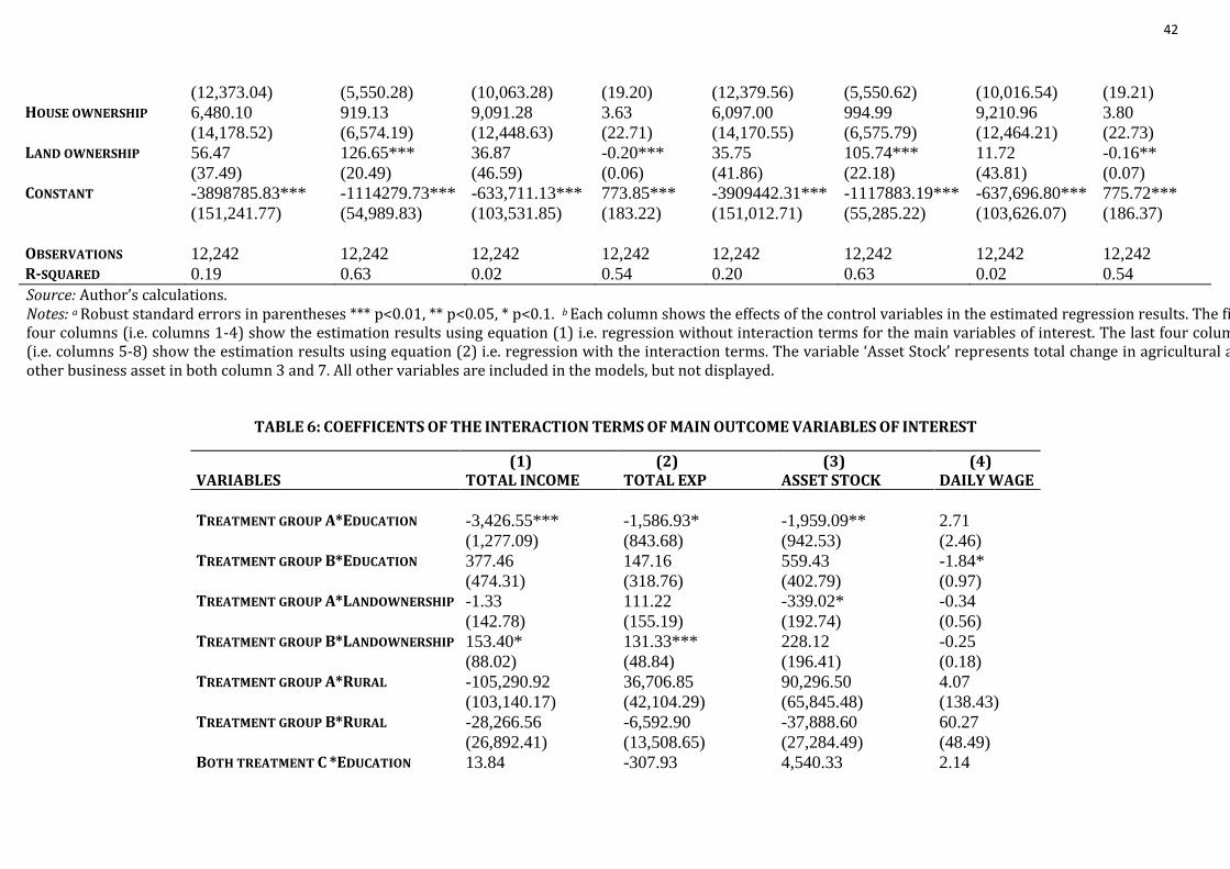
42
(12,373.04) (5,550.28) (10,063.28) (19.20) (12,379.56) (5,550.62) (10,016.54) (19.21) HOUSE OWNERSHIP 6,480.10 919.13 9,091.28 3.63 6,097.00 994.99 9,210.96 3.80 (14,178.52) (6,574.19) (12,448.63) (22.71) (14,170.55) (6,575.79) (12,464.21) (22.73) LAND OWNERSHIP 56.47 126.65*** 36.87 -0.20*** 35.75 105.74*** 11.72 -0.16** (37.49) (20.49) (46.59) (0.06) (41.86) (22.18) (43.81) (0.07) CONSTANT -3898785.83*** -1114279.73*** -633,711.13*** 773.85*** -3909442.31*** -1117883.19*** -637,696.80*** 775.72*** (151,241.77) (54,989.83) (103,531.85) (183.22) (151,012.71) (55,285.22) (103,626.07) (186.37) OBSERVATIONS 12,242 12,242 12,242 12,242 12,242 12,242 12,242 12,242 R-SQUARED 0.19 0.63 0.02 0.54 0.20 0.63 0.02 0.54
Source: Author’s calculations. Notes: a Robust standard errors in parentheses *** p<0.01, ** p<0.05, * p<0.1. b Each column shows the effects of the control variables in the estimated regression results. The first four columns (i.e. columns 1-4) show the estimation results using equation (1) i.e. regression without interaction terms for the main variables of interest. The last four columns (i.e. columns 5-8) show the estimation results using equation (2) i.e. regression with the interaction terms. The variable ‘Asset Stock’ represents total change in agricultural and other business asset in both column 3 and 7. All other variables are included in the models, but not displayed.
TABLE 6: COEFFICENTS OF THE INTERACTION TERMS OF MAIN OUTCOME VARIABLES OF INTEREST
(1) (2) (3) (4) VARIABLES TOTAL INCOME TOTAL EXP ASSET STOCK DAILY WAGE
TREATMENT GROUP A*EDUCATION -3,426.55*** -1,586.93* -1,959.09** 2.71 (1,277.09) (843.68) (942.53) (2.46) TREATMENT GROUP B*EDUCATION 377.46 147.16 559.43 -1.84* (474.31) (318.76) (402.79) (0.97) TREATMENT GROUP A*LANDOWNERSHIP -1.33 111.22 -339.02* -0.34 (142.78) (155.19) (192.74) (0.56) TREATMENT GROUP B*LANDOWNERSHIP 153.40* 131.33*** 228.12 -0.25 (88.02) (48.84) (196.41) (0.18) TREATMENT GROUP A*RURAL -105,290.92 36,706.85 90,296.50 4.07 (103,140.17) (42,104.29) (65,845.48) (138.43) TREATMENT GROUP B*RURAL -28,266.56 -6,592.90 -37,888.60 60.27 (26,892.41) (13,508.65) (27,284.49) (48.49) BOTH TREATMENT C *EDUCATION 13.84 -307.93 4,540.33 2.14

43
(3,046.68) (2,278.24) (3,247.31) (5.70) BOTH TREATMENT C *LANDOWNERSHIP 216.98 177.94 -187.55 -0.42 (475.39) (205.67) (197.76) (0.52) BOTH TREATMENT C *RURAL -285,759.28* -124,226.08 -254,137.66 540.58* (154,600.41) (95,121.54) (222,356.04) (290.29) CONSTANT -3909442.31*** -1117883.19*** -637,696.80*** 775.72*** (151,012.71) (55,285.22) (103,626.07) (186.37) OBSERVATIONS 12,242 12,242 12,242 12,242 R-SQUARED 0.20 0.63 0.02 0.54
Source: Author’s calculations. Notes: a Robust standard errors in parentheses *** p<0.01, ** p<0.05, * p<0.1. b Each column shows the coefficients of the
interaction terms in the estimated regression results of main outcome variables of interest (i.e. estimated using equation 2). The variable ‘Asset Stock’ represents total change in agricultural and other business asset in column 3. All other variables are included in the models, but not displayed.
APPENDIX
APPENDIX TABLE 1: KEY VARIABLES WITH DESCRIPTIVE STATISTICS (TREATMENT AND CONTROL GROUP A: SELF-REPORTED IDENTIFICATIONS)
VARIABLES TYPE MEAN STANDARD DEVIATION DESCRIPTION OF VARIABLES OUTCOME VARIABLES TREATMENT CONTROL TREATMENT CONTROL PER CAPITA TOTAL INCOME Continuous 911940.4 926187.1 606662.3 641924.1 Sum of per capita crop, non-crop, business and other incomes.
PER CAPITA CROP INCOME Continuous 194200.9 172257.1 120641.9 94183.72 Per capita income earned through selling of crops.
PER CAPITA NON-CROP INCOME Continuous 233546.5 248931.6 537408.4 543124.3 Per capita income earned through selling of livestock and poultry, livestock products, fish farming and fish capture and farm forestry.
PER CAPITA BUSINESS INCOME Continuous 468905.9 488696 255953.5 296302.3 Per capita net revenues earned from non-agricultural enterprises and rental income from agricultural assets.
PER CAPITA OTHER INCOME Continuous 15287.03 16796.23 31811.08 51837.51 Per capita income earned from other assets (e.g. stocks, bonds, jewellery etc.), rent, insurance, charity, gift, remittances, bank interest and social safety net.
PER CAPITA TOTAL Continuous 1454900 1441364 431931.9 434467.7 Sum of per capita food, non-food, crop, non-crop, agricultural

44
EXPENDITURE input, education and health expenditures.
PER CAPITA FOOD
EXPENDITURE Continuous 85007.71 85364.12 23346.4 22095.96 Per capita daily and weekly food consumption.
PER CAPITA NON-FOOD
EXPENDITURE Continuous 737893.7 742763.1 236691.1 242337.5 Per capita monthly and annual non-food consumption.
PER CAPITA CROP
EXPENDITURE Continuous 107859.9 106216.5 41673.97 46624.14 Per capita crop consumption by household.
PER CAPITA NON-CROP
EXPENDITURE Continuous 96695 92351.51 62587.95 46292.79 Per capita consumption of livestock and poultry, livestock
products, fish farming and fish capture and farm forestry products by household.
PER CAPITA AGRICULTURAL
INPUT EXPENDITURE Continuous 292600.7 285233.4 132586.7 129633 Per capita expenses on agricultural inputs.
PER CAPITA EDUCATIONAL
EXPENDITURE Continuous 121299.4 118282.5 60326.1 56320.71 Per capita expenditure for educational services.
PER CAPITA HEALTH
EXPENDITURE Continuous 13543.29 11406.69 21518.79 12382.97 Per capita expenditure for health services.
TOTAL CHANGE IN
AGRICULTURAL AND OTHER
BUSINESS ASSET (IN REAL
TERMS)
Continuous 174977.2 185579.5 491300.3 497618.8 Sum of agricultural assets households bought in the last 12 months and expenditure in capital goods (in non-agricultural enterprises) in the last 12 months.
TOTAL AGRICULTURAL INPUT
ASSET VALUE (IN REAL TERMS) Continuous 222404.2 237534.1 221172.2 248540 Value of owned equipment and asset used in agriculture.
TOTAL CONSUMER DURABLE
ASSET VALUE (IN REAL TERMS) Continuous 2976063 3019571 1500622 1413280 Total asset value of consumer durable goods.
TOTAL MONTH PER YEAR
WORKED Continuous 801.2356 806.6025 227.3714 217.8752 Total number of months per year worked.
TOTAL DAYS PER MONTH
WORKED Continuous 1784.529 1800.281 512.2758 489.88 Total number of days per month worked.
TOTAL HOURS PER DAY
WORKED Continuous 617.1022 621.6139 174.0195 166.3709 Total number of hours per day worked.
DAILY WAGE (IN REAL TERMS) Continuous 3852.178 3941.571 1414.781 1354.073 Daily wage in cash (if paid daily).
SALARIED WAGE (IN REAL
TERMS) Continuous 108128.6 105938.3 50919.97 47547.04 Total net take-home monthly remuneration after all deduction
at source. YEARLY BENEFITS (IN REAL
TERMS) Continuous 138585.8 134053.7 90501.7 88512.07 Total value of yearly in-kind or other benefits (tips, bonuses or
transport) from employment. COVARIATES

45
RURAL Binary 0.675556 0.63976 0.469211 0.48009 Whether living in a rural area = 1, otherwise 0.
HEAD OF HOUSEHOLD IS MALE Binary 1.004444 1.003994 0.066667 0.066918 Whether head of the household is male = 1, otherwise 0.
AVERAGE AGE Continuous 26.4378 26.67 1.347331 1.386957 Average age of household members.
DEPENDENT Continuous 90.41333 90.62736 24.58355 24.16744 Age of the household member is <15 and >=65.
PROPORTION OF FORMAL
EDUCATION Continuous 76.81407 76.97305 19.83074 19.25972 Proportion of household members attended school, college,
university or madrasa. ACCESS TO SANITATION Binary 0.488889 0.528168 0.500991 0.499227 Whether the household use sanitary or pacca latrines (water
seal and pit) = 1, otherwise 0. ACCESS TO SAFE DRINKING
WATER Binary 0.991111 0.963968 0.09407 0.186378 Whether the household has access to supply water or tube well
water = 1, otherwise 0. ACCESS TO ELECTRICITY Binary 0.608889 0.575934 0.489087 0.494221 Whether the household has got electricity connection = 1,
otherwise 0. HOUSE OWNERSHIP Binary 0.857778 0.809603 0.350057 0.392631 Whether the household own a house = 1, otherwise 0.
LAND OWNERSHIP (IN REAL
TERMS) Continuous 69.48 62.74894 128.0451 128.9109 Amount of total operating land (in acres).
Source: Author’s calculations and elaborations.
APPENDIX TABLE 2: KEY VARIABLES WITH DESCRIPTIVE STATISTICS (TREATMENT AND CONTROL GROUP B: RAINFALL-BASED IDENTIFICATIONS)
VARIABLES TYPE MEAN STANDARD DEVIATION DESCRIPTION OF VARIABLES OUTCOME VARIABLES TREATMENT CONTROL TREATMENT CONTROL PER CAPITA TOTAL INCOME Continuous 910175.2 928971.5 581756.4 652139.9 Sum of per capita crop, non-crop, business and other incomes.
PER CAPITA CROP INCOME Continuous 169420 173286.1 91191.19 95445.03 Per capita income earned through selling of crops.
PER CAPITA NON-CROP INCOME Continuous 230389.3 252173 456983.5 558031.4 Per capita income earned through selling of livestock and poultry, livestock products, fish farming and fish capture and farm forestry.
PER CAPITA BUSINESS INCOME Continuous 493480 487336.6 303387.3 294090.6 Per capita net revenues earned from non-agricultural enterprises and rental income from agricultural assets.
PER CAPITA OTHER INCOME Continuous 18149.76 16501.34 66344.03 48152.93 Per capita income earned from other assets (e.g. stocks, bonds, jewellery etc.), rent, insurance, charity, gift, remittances, bank interest and social safety net.
PER CAPITA TOTAL EXPENDITURE Continuous 1426657 1444506 431057.4 435013.9 Sum of per capita food, non-food, crop, non-crop, agricultural input, education and health expenditures.
PER CAPITA FOOD EXPENDITURE Continuous 85224.26 85383.35 22023.35 22137.98 Per capita daily and weekly food consumption.

46
PER CAPITA NON-FOOD
EXPENDITURE Continuous 736179.2 743929.7 243034.8 242061.4 Per capita monthly and annual non-food consumption.
PER CAPITA CROP EXPENDITURE Continuous 105621.7 106367.3 47004.28 46447.4 Per capita crop consumption by household.
PER CAPITA NON-CROP
EXPENDITURE Continuous 92745.11 92370.86 48930.08 46192.2 Per capita consumption of livestock and poultry, livestock
products, fish farming and fish capture and farm forestry products by household.
PER CAPITA AGRICULTURAL INPUT
EXPENDITURE Continuous 278433.5 286710.1 126025.8 130345.6 Per capita expenses on agricultural inputs.
PER CAPITA EDUCATIONAL
EXPENDITURE Continuous 117582.6 118484 55490.5 56570.64 Per capita expenditure for educational services.
PER CAPITA HEALTH EXPENDITURE Continuous 11530.68 11429.57 13545.26 12424.67 Per capita expenditure for health services.
TOTAL CHANGE IN AGRICULTURAL
AND OTHER BUSINESS ASSET (IN
REAL TERMS)
Continuous 188845 184715.4 504566.3 496126.6 Sum of agricultural assets households bought in the last 12 months and expenditure in capital goods (in non-agricultural enterprises) in the last 12 months.
TOTAL AGRICULTURAL INPUT ASSET
VALUE (IN REAL TERMS) Continuous 232030.2 238266.7 225549.4 252185 Value of owned equipment and asset used in agriculture.
TOTAL CONSUMER DURABLE ASSET
VALUE (IN REAL TERMS) Continuous 3037415 3015165 1413003 1415285 Total asset value of consumer durable goods.
TOTAL MONTH PER YEAR WORKED Continuous 808.5736 806.1035 214.9811 218.6407 Total number of months per year worked.
TOTAL DAYS PER MONTH WORKED Continuous 1807.041 1798.628 487.7013 490.7934 Total number of days per month worked.
TOTAL HOURS PER DAY WORKED Continuous 622.7273 621.2996 165.55 166.7001 Total number of hours per day worked.
DAILY WAGE (IN REAL TERMS) Continuous 3965.141 3935.052 1331.947 1359.669 Daily wage in cash (if paid daily).
SALARIED WAGE (IN REAL TERMS) Continuous 105521 106067.1 47314.31 47668.63 Total net take-home monthly remuneration after all deduction at source.
YEARLY BENEFITS (IN REAL TERMS) Continuous 131762.1 134596.3 88682.74 88518.13 Total value of yearly in-kind or other benefits (tips, bonuses or transport) from employment.
COVARIATES
RURAL Binary 0.626008 0.643205 0.483984 0.479077 Whether living in a rural area = 1, otherwise 0.
HEAD OF HOUSEHOLD IS MALE Binary 1.00252 1.004289 0.067322 0.066831 Whether head of the household is male = 1, otherwise 0.
AVERAGE AGE Continuous 26.63367 26.67193 1.643582 1.331109 Average age of household members.
DEPENDENT Continuous 90.70716 90.60723 24.26731 24.15725 Age of the household member is <15 and >=65.
PROPORTION OF FORMAL
EDUCATION Continuous 76.95353 76.97334 19.29904 19.26478 Proportion of household members attended school, college,
university or madrasa. ACCESS TO SANITATION Binary 0.524194 0.528076 0.49954 0.499236 Whether the household use sanitary or pacca latrines (water
seal and pit) = 1, otherwise 0.

47
ACCESS TO SAFE DRINKING WATER Binary 0.970262 0.963346 0.169906 0.187921 Whether the household has access to supply water or tube well water = 1, otherwise 0.
ACCESS TO ELECTRICITY Binary 0.571573 0.577501 0.494976 0.493981 Whether the household has got electricity connection = 1, otherwise 0.
HOUSE OWNERSHIP Binary 0.806452 0.811269 0.395179 0.391314 Whether the household own a house = 1, otherwise 0.
LAND OWNERSHIP (IN REAL TERMS) Continuous 61.85938 63.06863 121.0524 130.3597 Amount of total operating land (in acres).
Source: Author’s calculations and elaborations.
APPENDIX TABLE 3: IMPACT ON HOUSEHOLD INCOME PER CAPITA
(1) (2) (3) (4) (5) VARIABLES TOTAL INCOME CROP INCOME NON-CROP INCOME BUSINESS INCOME OTHER INCOME
TREATMENT GROUP A 332,832.82** 142,294.50** 109,491.86 78,193.44 6,665.53 (SELF-REPORT) (130,063.55) (66,072.70) (93,443.48) (59,470.25) (7,903.15) TREATMENT GROUP B -32,407.34 -13,883.61* -41,104.20* 2,247.68 1,127.58 (RAINFALL-BASED) (40,347.94) (7,825.42) (23,314.76) (23,700.09) (4,797.41) BOTH TREATMENT GROUP C 250,726.57 -34,353.69 71,339.47 212,991.08 4,037.39 (250,456.37) (31,556.09) (108,105.23) (289,247.54) (9,569.99) RURAL 10,588.13 2,848.28 11,912.35 -2,120.64 -3,122.61** (14,485.90) (2,177.35) (12,997.85) (6,267.27) (1,264.07) MALE HEADED HH 2,368,798.65*** 11,914.41*** 2,490,203.56*** -78,471.56*** 36,387.45 (71,878.91) (1,669.76) (10,589.02) (4,771.17) (36,918.57) AVG AGE 57,682.42*** 1,698.52*** 54,323.07*** 1,159.21 522.45* (5,132.86) (604.68) (5,414.47) (1,798.51) (301.25) DEPENDENT -90.86 101.30 4,633.54*** -4,768.54*** -7.79 (727.59) (97.28) (557.06) (516.23) (52.47) PROPORTION_FORMAL EDUCATION 11,341.01*** 1,581.53*** -2,684.13*** 12,438.64*** -9.55 (872.70) (122.12) (646.46) (646.73) (63.21) ACCESS_SANITATION 43,113.45*** 5,138.40*** 17,808.24* 6,257.87 13,642.42*** (11,035.25) (1,749.42) (9,757.08) (5,074.56) (808.18) ACCESS_DRINKING WATER 17,789.45 -4,721.25 2,483.01 16,305.28 3,296.77** (28,262.85) (4,847.53) (25,741.41) (11,427.32) (1,373.56) ACCESS_ELECTRICITY 3,523.53 2,720.74 -7,322.33 -4,293.78 11,884.05***

48
(12,379.56) (1,878.93) (11,128.56) (5,419.89) (827.41) HOUSE OWNERSHIP 6,097.00 1,485.33 1,106.72 -2,103.23 6,006.25*** (14,170.55) (2,212.30) (12,431.79) (6,588.55) (1,335.07) LAND OWNERSHIP 35.75 51.92*** -38.66 2.29 21.41*** (41.86) (10.05) (35.27) (19.71) (3.54) INTERACTION_EDU*SELF -3,426.55*** -1,541.98* -547.17 -1,246.72 -138.35 (1,277.09) (797.44) (528.88) (769.64) (102.86) INTERACTION_EDU*RAIN 377.46 73.70 277.13 143.83 89.13 (474.31) (100.56) (231.69) (314.11) (64.34) INTERACTION_LAND*SELF -1.33 -73.89 26.56 74.79 -27.98** (142.78) (51.88) (117.67) (85.74) (11.88) INTERACTION_LAND*RAIN 153.40* 19.84 65.61 79.40 -11.00* (88.02) (18.30) (63.88) (53.63) (6.47) INTERACTION_RURAL*SELF -105,290.92 4,794.74 -109,936.88 -6,766.19 6,706.57 (103,140.17) (17,866.76) (98,365.55) (36,778.21) (4,377.83) INTERACTION_RURAL*RAIN -28,266.56 5,564.84 -2,883.13 -18,448.15 -8,784.48** (26,892.41) (4,424.02) (22,237.89) (14,453.90) (3,935.12) INTERACTION_EDU*BOTH 13.84 600.20 -534.65 -112.16 19.12 (3,046.68) (523.88) (1,343.91) (3,118.24) (181.29) INTERACTION_LAND*BOTH 216.98 -74.37** 151.12 143.02 -4.19 (475.39) (37.38) (112.73) (433.10) (18.90) INTERACTION_RURAL*BOTH -285,759.28* -21,735.52 -87,400.23 -168,448.08 -7,538.56 (154,600.41) (31,745.12) (87,197.53) (113,814.19) (14,271.53) CONSTANT -3909442.31*** -21,563.08 -3924719.01*** -3,824.37 -53,964.73 (151,012.71) (18,140.35) (134,578.19) (47,057.14) (40,194.24) OBSERVATIONS 12,242 12,222 12,232 12,242 12,242 R-SQUARED 0.20 0.13 0.12 0.21 0.05
Source: Author’s calculations. Note: Robust standard errors in parentheses *** p<0.01, ** p<0.05, * p<0.1.

49
APPENDIX TABLE 4: IMPACT ON HOUSEHOLD EXPENDITURE PER CAPITA
(1) (2) (3) (4) (5) (6) (7) (8) VARIABLES TOTAL EXP FOOD EXP NON-FOOD EXP CROP EXP NON-CROP EXP AGRI INPUT EXP EDU EXP HEALTH EXP
TREATMENT GROUP A 109,304.40 -893.17 24,065.29 21,798.01*** 23,606.10 29,781.65 8,633.44 3,046.33 (SELF-REPORT) (66,457.58) (1,842.23) (38,785.57) (7,093.41) (32,813.66) (26,748.11) (11,254.61) (3,285.08) TREATMENT GROUP B -30,077.56 -471.48 -28,168.21** -3,412.53 9,460.94 -3,632.92 -3,452.94 204.28 (RAINFALL-BASED) (24,804.11) (585.81) (14,352.09) (2,967.95) (8,839.87) (9,704.29) (3,460.80) (856.08) BOTH TREATMENT GROUP C 110,647.41 -975.08 8,624.64 -11,033.88 37,025.74* 82,551.46 -17,473.19 12,004.26 (190,050.55) (3,115.48) (90,739.61) (12,885.29) (21,240.47) (81,685.85) (20,801.70) (13,917.93) RURAL -1,802.73 -242.36 -3,407.63 373.74 1,560.82* 1,948.22 -2,257.43** 189.02 (6,285.55) (150.46) (3,971.61) (883.11) (913.55) (2,598.06) (1,143.68) (267.27) MALE HEADED HH 391,391.05*** 5,186.41*** 3,699.66 34,917.76*** 42,366.12*** 303,488.83*** -2,049.84* 2,951.47*** (18,671.89) (460.12) (9,928.50) (757.43) (709.18) (8,601.82) (1,108.28) (324.14) AVG AGE 29,159.82*** 671.78*** 11,272.68*** 2,159.28*** 3,988.52*** 13,060.39*** -1,233.69*** -305.68*** (2,415.98) (61.62) (1,386.27) (311.37) (264.12) (933.72) (302.28) (59.24) DEPENDENT -2,399.32*** -166.58*** -2,661.61*** -316.63*** 234.31*** 1,625.64*** -1,087.52*** 2.60 (341.96) (10.28) (180.25) (99.47) (44.56) (134.08) (53.06) (11.00) PROPORTION_FORMAL
EDUCATION 20,513.60*** 1,292.96*** 12,034.98*** 1,806.85*** 928.99*** 1,549.82*** 2,741.30*** 128.32***
(420.18) (12.64) (222.66) (124.28) (63.13) (163.31) (62.75) (12.46) ACCESS_SANITATION 17,293.25*** 117.35 6,720.77** 1,167.83 1,946.89** 6,901.97*** 741.57 -347.54 (5,193.54) (125.61) (3,316.55) (725.81) (796.11) (2,103.76) (932.48) (237.55) ACCESS_DRINKING WATER 9,517.59 273.53 3,805.46 2,711.73 1,026.78 1,442.23 124.06 141.81 (13,168.53) (316.18) (8,210.24) (1,843.18) (2,367.63) (5,550.99) (2,551.95) (532.75) ACCESS_ELECTRICITY 8,420.74 376.49*** 8,771.70** 56.34 414.91 -1,847.10 241.60 338.17 (5,550.62) (133.52) (3,524.65) (763.14) (837.94) (2,274.92) (998.96) (262.60) HOUSE OWNERSHIP 994.99 -166.91 806.85 1,243.84 718.72 -662.14 -1,317.05 372.74 (6,575.79) (158.83) (4,179.84) (950.78) (960.10) (2,642.09) (1,261.40) (269.49) LAND OWNERSHIP 105.74*** 1.98*** 15.31 19.06*** 9.50*** 53.11*** 7.21* -0.46 (22.18) (0.50) (12.64) (3.48) (3.03) (10.65) (3.96) (0.76) INTERACTION_EDU*SELF -1,586.93* 7.00 -587.34 -240.48*** -314.78 -354.30 -69.40 -36.78 (843.68) (22.81) (477.28) (85.77) (434.43) (337.07) (115.75) (38.18) INTERACTION_EDU*RAIN 147.16 1.96 249.64 34.98 -104.70 -67.41 35.44 -8.49

50
(318.76) (7.56) (184.61) (43.20) (104.74) (122.33) (42.05) (9.42) INTERACTION_LAND*SELF 111.22 3.04 101.79 18.53 -18.21 42.81 -25.66 -11.37 (155.19) (3.91) (81.16) (14.57) (20.41) (90.36) (19.28) (7.65) INTERACTION_LAND*RAIN 131.33*** -0.78 68.11* 8.54 15.11* 21.03 17.64** 1.50 (48.84) (1.30) (34.78) (10.04) (8.14) (22.58) (8.04) (2.26) INTERACTION_RURAL*SELF 36,706.85 117.90 17,354.04 -3,606.60 10,884.55 6,127.46 2,088.09 3,912.85 (42,104.29) (1,053.46) (24,960.06) (5,193.34) (8,662.20) (15,892.27) (8,463.01) (2,734.17) INTERACTION_RURAL*RAIN -6,592.90 443.68 -3,455.71 -941.26 -2,704.26 879.13 -1,783.21 827.14 (13,508.65) (323.38) (8,710.50) (2,028.72) (2,307.33) (5,467.69) (2,477.04) (635.08) INTERACTION_EDU*BOTH -307.93 10.76 255.17 197.26 -425.43 -469.93 261.43 -139.77 (2,278.24) (40.58) (1,209.62) (179.59) (267.90) (964.24) (272.62) (177.90) INTERACTION_LAND*BOTH 177.94 -9.56* 295.31** 18.03 14.48 -135.72** 11.18 -15.51 (205.67) (4.89) (127.41) (25.91) (16.14) (61.45) (62.09) (21.35) INTERACTION_RURAL*BOTH -124,226.08 -1,021.28 -86,641.55* -8,501.37 -2,720.75 -26,390.71 -4,019.46 5,161.58 (95,121.54) (1,850.98) (50,266.06) (11,330.75) (10,575.23) (55,480.81) (11,952.45) (8,642.57) CONSTANT -1117883.19*** -22,543.11*** -257,255.92*** -102,577.12*** -153,919.47*** -641,350.11*** 42,321.43*** 5,901.83*** (55,285.22) (1,394.69) (31,353.61) (8,307.50) (8,140.76) (23,813.61) (8,316.00) (1,793.13) OBSERVATIONS 12,242 12,242 12,242 12,222 12,232 12,242 12,242 12,242 R-SQUARED 0.63 0.92 0.52 0.36 0.25 0.31 0.27 0.04
Source: Author’s calculations. Note: Robust standard errors in parentheses *** p<0.01, ** p<0.05, * p<0.1.
APPENDIX TABLE 5: IMPACT ON TOTAL ASSET OUTCOMES
(1) (2) (3) VARIABLES ASSET STOCK AGRI INPUT ASSET VALUE DURABLE ASSET VALUE
TREATMENT GROUP A 111,132.59 90,455.01* -256,836.22 (SELF-REPORT) (75,127.02) (47,600.49) (220,139.63) TREATMENT GROUP B -28,898.86 3,374.68 -7,225.67 (RAINFALL-BASED) (30,787.83) (15,521.03) (91,144.36) BOTH TREATMENT GROUP C -178,097.20* -82,060.72 -291,623.55 (101,758.84) (57,755.00) (469,256.70)

51
RURAL -14,252.62 -71.63 -61,639.28** (11,702.90) (5,656.31) (29,687.66) MALE HEADED HH -8,218.23 40,935.76*** 504,722.21*** (22,034.97) (3,894.96) (36,784.03) AVG AGE 25,416.28*** 4,417.15*** 42,026.79*** (4,157.71) (1,346.94) (8,571.44) DEPENDENT 5,228.63*** 2,944.75*** -6,514.56*** (790.41) (229.34) (1,579.32) PROPORTION_FORMAL
EDUCATION -3,649.11*** -183.31 42,871.98***
(945.78) (281.99) (1,981.59) ACCESS_SANITATION 4,299.30 1,113.03 62,287.27*** (9,519.76) (4,791.74) (24,043.79) ACCESS_DRINKING WATER -38,126.05 3,462.39 -112,338.24 (28,610.75) (11,583.60) (72,140.41) ACCESS_ELECTRICITY -8,129.74 3,359.32 2,443.59 (10,016.54) (5,031.24) (25,963.45) HOUSE OWNERSHIP 9,210.96 11,980.88** -22,809.59 (12,464.21) (5,625.60) (31,497.00) LAND OWNERSHIP 11.72 43.39* 104.46 (43.81) (23.22) (108.47) INTERACTION_EDU*SELF -1,959.09** -1,482.33** -53.84 (942.53) (597.10) (2,847.95) INTERACTION_EDU*RAIN 559.43 -69.95 239.14 (402.79) (212.63) (1,135.26) INTERACTION_LAND*SELF -339.02* -1.56 -78.07 (192.74) (121.02) (664.81) INTERACTION_LAND*RAIN 228.12 -11.03 319.24 (196.41) (43.53) (357.72) INTERACTION_RURAL*SELF 90,296.50 11,563.94 369,207.02** (65,845.48) (29,702.03) (162,794.83) INTERACTION_RURAL*RAIN -37,888.60 -6,252.62 -9,190.84 (27,284.49) (11,606.95) (66,058.85) INTERACTION_EDU*BOTH 4,540.33 476.40 3,673.89 (3,247.31) (801.11) (5,963.49)
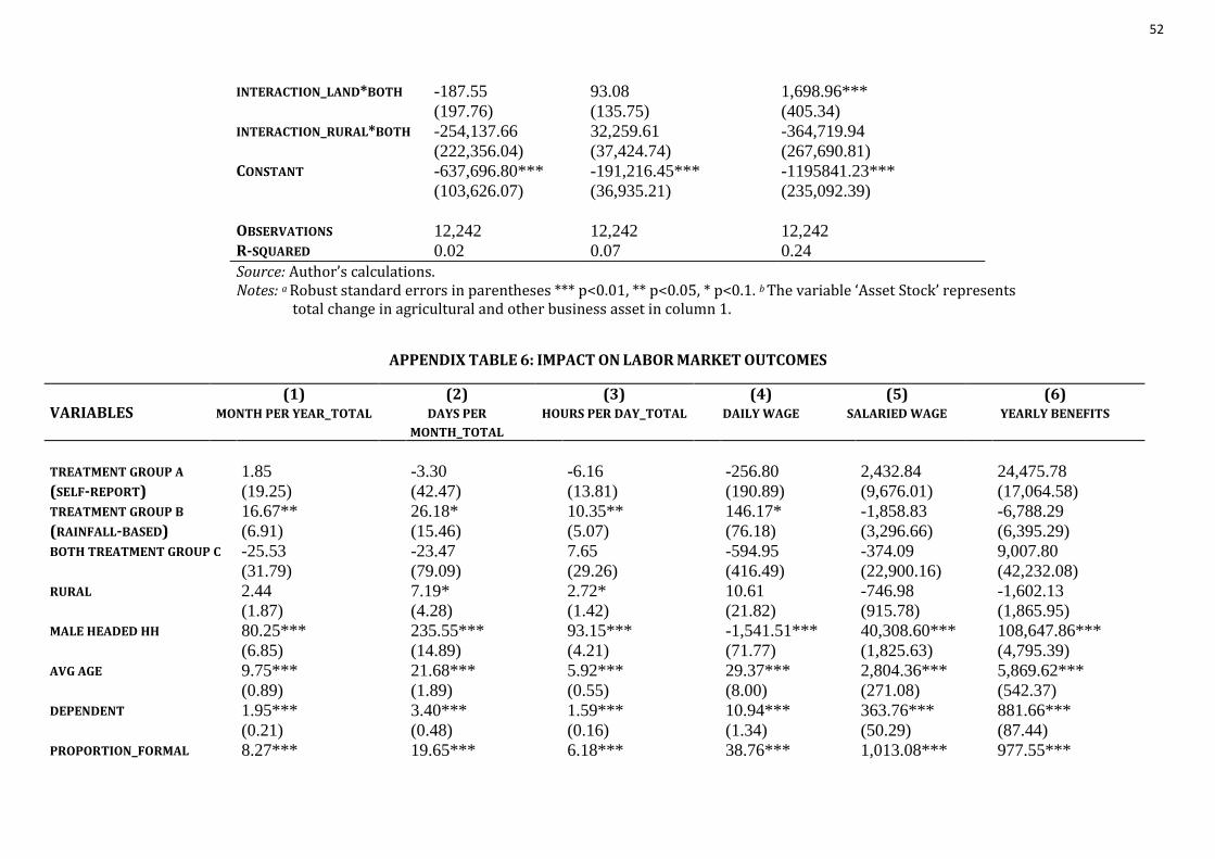
52
INTERACTION_LAND*BOTH -187.55 93.08 1,698.96*** (197.76) (135.75) (405.34) INTERACTION_RURAL*BOTH -254,137.66 32,259.61 -364,719.94 (222,356.04) (37,424.74) (267,690.81) CONSTANT -637,696.80*** -191,216.45*** -1195841.23*** (103,626.07) (36,935.21) (235,092.39) OBSERVATIONS 12,242 12,242 12,242 R-SQUARED 0.02 0.07 0.24
Source: Author’s calculations. Notes: a Robust standard errors in parentheses *** p<0.01, ** p<0.05, * p<0.1. b The variable ‘Asset Stock’ represents
total change in agricultural and other business asset in column 1.
APPENDIX TABLE 6: IMPACT ON LABOR MARKET OUTCOMES
(1) (2) (3) (4) (5) (6) VARIABLES MONTH PER YEAR_TOTAL DAYS PER
MONTH_TOTAL HOURS PER DAY_TOTAL DAILY WAGE SALARIED WAGE YEARLY BENEFITS
TREATMENT GROUP A 1.85 -3.30 -6.16 -256.80 2,432.84 24,475.78 (SELF-REPORT) (19.25) (42.47) (13.81) (190.89) (9,676.01) (17,064.58) TREATMENT GROUP B 16.67** 26.18* 10.35** 146.17* -1,858.83 -6,788.29 (RAINFALL-BASED) (6.91) (15.46) (5.07) (76.18) (3,296.66) (6,395.29) BOTH TREATMENT GROUP C -25.53 -23.47 7.65 -594.95 -374.09 9,007.80 (31.79) (79.09) (29.26) (416.49) (22,900.16) (42,232.08) RURAL 2.44 7.19* 2.72* 10.61 -746.98 -1,602.13 (1.87) (4.28) (1.42) (21.82) (915.78) (1,865.95) MALE HEADED HH 80.25*** 235.55*** 93.15*** -1,541.51*** 40,308.60*** 108,647.86*** (6.85) (14.89) (4.21) (71.77) (1,825.63) (4,795.39) AVG AGE 9.75*** 21.68*** 5.92*** 29.37*** 2,804.36*** 5,869.62*** (0.89) (1.89) (0.55) (8.00) (271.08) (542.37) DEPENDENT 1.95*** 3.40*** 1.59*** 10.94*** 363.76*** 881.66*** (0.21) (0.48) (0.16) (1.34) (50.29) (87.44) PROPORTION_FORMAL 8.27*** 19.65*** 6.18*** 38.76*** 1,013.08*** 977.55***

53
EDUCATION (0.26) (0.60) (0.19) (1.66) (61.96) (109.81) ACCESS_SANITATION -3.91** -5.70 -1.61 -42.27** -642.50 -3,830.55** (1.54) (3.51) (1.16) (17.96) (749.87) (1,542.10) ACCESS_DRINKING WATER -4.00 -0.98 -1.44 -36.23 3,331.43* 4,005.18 (4.02) (9.27) (3.19) (45.58) (1,819.89) (3,773.47) ACCESS_ELECTRICITY 1.86 3.36 1.17 15.70 2,218.86*** 5,551.05*** (1.64) (3.74) (1.24) (19.21) (807.38) (1,658.07) HOUSE OWNERSHIP -4.60** -12.83*** -4.33*** 3.80 -2,863.53*** -3,400.65* (1.94) (4.47) (1.48) (22.73) (969.74) (1,966.14) LAND OWNERSHIP 0.02** 0.03* 0.01* -0.16** 0.43 -6.40 (0.01) (0.02) (0.01) (0.07) (2.82) (5.51) INTERACTION_EDU*SELF -0.08 -0.05 0.04 2.71 -5.69 -150.66 (0.25) (0.56) (0.18) (2.46) (123.02) (223.76) INTERACTION_EDU*RAIN -0.15 -0.17 -0.10 -1.84* 17.09 16.48 (0.09) (0.21) (0.07) (0.97) (43.89) (83.51) INTERACTION_LAND*SELF 0.03 0.09 0.01 -0.34 33.03 109.46* (0.04) (0.09) (0.02) (0.56) (21.64) (58.92) INTERACTION_LAND*RAIN -0.02 -0.02 -0.01 -0.25 8.52 36.01** (0.02) (0.04) (0.01) (0.18) (7.21) (17.08) INTERACTION_RURAL*SELF 1.96 -7.12 0.17 4.07 -1,947.38 -22,003.46* (11.68) (26.72) (8.60) (138.43) (6,181.85) (12,776.98) INTERACTION_RURAL*RAIN -1.58 -2.77 0.17 60.27 -545.85 1,437.62 (4.25) (9.94) (3.32) (48.49) (1,995.69) (4,105.48) INTERACTION_EDU*BOTH 0.08 -0.11 -0.34 2.14 -5.49 -211.64 (0.39) (1.03) (0.37) (5.70) (332.72) (573.90) INTERACTION_LAND*BOTH 0.09** 0.06 0.03 -0.42 17.67 63.62 (0.04) (0.10) (0.03) (0.52) (34.77) (97.04) INTERACTION_RURAL*BOTH -1.31 19.23 10.85 540.58* -447.52 17,898.27 (23.68) (54.57) (17.32) (290.29) (14,984.88) (25,735.38) CONSTANT -341.74*** -831.20*** -247.55*** 775.72*** -121,591.01*** -287,205.30*** (20.36) (45.04) (13.93) (186.37) (7,032.51) (14,982.38) OBSERVATIONS 12,242 12,242 12,242 12,242 12,242 12,242

54
R-SQUARED 0.87 0.87 0.87 0.54 0.35 0.21
Source: Author’s calculations. Note: Robust standard errors in parentheses *** p<0.01, ** p<0.05, * p<0.1.
APPENDIX TABLE 7: IMPACT ON HOUSEHOLD INCOME PER CAPITA (ROBUSTNESS CHECKS)
(1) (2) (3) (4) (5) VARIABLES TOTAL INCOME CROP INCOME NON-CROP INCOME BUSINESS INCOME OTHER INCOME
RAINFALL-BASED TREATMENT GROUP 10,225.32 -1,670.12 2,504.74 8,684.94* 4,942.52 (7,873.66) (2,287.10) (8,157.23) (5,218.46) (3,241.37) RURAL 3,826.76 1,843.09 6,906.42 -2,742.50 -2,366.68** (9,563.84) (1,771.04) (9,458.35) (4,844.04) (962.72) MALE HEADED HH 106,190.04*** 4,279.77*** 156,315.88*** -5,036.55* -15,297.99*** (15,454.73) (498.48) (20,270.46) (2,910.89) (2,542.05) AVG AGE 1,229.06*** 123.71*** 1,341.71*** -303.98*** 352.41** (184.92) (25.66) (122.21) (75.12) (153.94) DEPENDENT -4,684.33*** -13.21 44.39 -4,684.31*** -89.25* (527.99) (88.52) (306.13) (464.95) (52.48) PROPORTION_FORMAL EDUCATION 16,788.64*** 1,699.21*** 2,730.44*** 12,318.84*** 105.94* (638.38) (116.66) (370.16) (577.17) (61.70) ACCESS_SANITATION 28,361.03*** 3,757.93*** 9,622.42* 6,950.32** 12,395.65*** (5,839.73) (1,116.63) (5,636.50) (3,141.17) (661.46) ACCESS_DRINKING WATER 9,251.90 -2,119.32 3,675.13 9,253.10 1,255.88 (14,324.94) (3,048.48) (14,606.39) (7,150.69) (1,009.04) ACCESS_ELECTRICITY 8,490.24 2,503.22** -4,780.99 883.74 11,592.06*** (6,403.19) (1,181.74) (6,285.21) (3,342.68) (554.27) HOUSE OWNERSHIP 11,404.29 1,779.07 7,090.97 -2,421.60 3,523.03 (8,474.06) (1,955.37) (9,531.14) (4,900.32) (2,249.82) LAND OWNERSHIP 48.88 52.14*** -28.24 4.27 21.87*** (41.01) (9.84) (34.77) (19.19) (3.49) INTERACTION_EDU*RAIN -309.70* -59.93* -320.86** 54.45 14.54 (183.39) (32.74) (150.39) (100.45) (29.87) INTERACTION_LAND*RAIN 122.67 16.54 64.23 66.93 -19.69***

55
(87.21) (17.75) (64.00) (51.85) (7.59) INTERACTION_RURAL*RAIN -9,898.18 3,256.91 -3,842.42 -11,769.63* -4,200.86 (10,316.34) (2,531.01) (10,339.58) (6,190.84) (2,863.08) YEAR_2005 -20,867.16* -35,071.41*** -25,279.97*** 56,376.63*** -1,749.41 (11,710.74) (4,010.14) (7,315.96) (8,798.92) (1,637.47) YEAR_2000 -14,153.68 -34,754.37*** -28,506.92*** 50,629.27*** 4,099.21 (12,073.87) (4,025.72) (7,217.83) (8,719.09) (3,214.16) CONSTANT -122,649.37*** 28,543.27*** -169,272.72*** -33,435.61*** 5,134.42 (25,963.04) (5,833.17) (27,998.96) (11,865.19) (5,655.63) OBSERVATIONS 26,151 19,859 23,448 21,278 26,138 R-SQUARED 0.56 0.59 0.10 0.61 0.03
Source: Author’s calculations. Note: Robust standard errors in parentheses *** p<0.01, ** p<0.05, * p<0.1.
APPENDIX TABLE 8: IMPACT ON HOUSEHOLD EXPENDITURE PER CAPITA (ROBUSTNESS CHECKS)
(1) (2) (3) (4) (5) (6) (7) (8) VARIABLES TOTAL EXP FOOD EXP NON-FOOD EXP CROP EXP NON-CROP EXP AGRI INPUT EXP EDU EXP HEALTH EXP
RAINFALL-BASED
TREATMENT GROUP -4,656.43 -367.75*** -3,689.06* 277.05 1,191.28 752.44 -287.93 -70.93
(3,414.86) (80.62) (2,151.86) (952.88) (874.69) (2,382.13) (755.07) (187.49) RURAL -2,543.96 -221.98** -4,091.06 479.68 1,250.45* 1,318.86 -1,681.34** 279.81 (4,087.69) (97.71) (2,554.35) (710.74) (651.19) (2,082.45) (833.69) (203.10) MALE HEADED HH 21,844.85*** 206.50*** -461.06 5,854.54*** 3,521.09*** 37,313.59*** -808.63 246.11*** (2,628.08) (41.00) (513.14) (646.85) (388.41) (4,436.65) (504.88) (47.47) AVG AGE 353.18*** 1.66* 51.29** 73.47*** 85.84*** 481.79*** -78.95*** -4.05* (37.79) (0.97) (22.48) (13.26) (6.16) (32.38) (16.48) (2.07) DEPENDENT -4,256.53*** -199.48*** -3,248.27*** -456.44*** -37.46 660.52*** -998.22*** 19.53** (306.31) (8.72) (166.45) (84.40) (42.60) (121.75) (51.35) (8.71) PROPORTION_FORMAL
EDUCATION 22,643.13*** 1,329.00*** 12,714.95*** 1,969.87*** 1,217.45*** 2,667.67*** 2,645.65*** 107.05***
(377.51) (10.72) (202.46) (106.54) (65.13) (148.95) (59.62) (10.10) ACCESS_SANITATION 9,030.51*** -64.67 3,775.33** 767.22* 1,111.87** 4,752.73*** 710.58 -184.06

56
(2,645.33) (63.91) (1,672.77) (464.68) (441.19) (1,324.98) (569.22) (152.42) ACCESS_DRINKING WATER 4,777.74 73.72 1,536.55 1,559.91 684.82 1,623.33 111.43 167.40 (6,551.77) (158.35) (4,055.80) (1,165.84) (1,302.12) (3,462.36) (1,587.77) (359.83) ACCESS_ELECTRICITY 4,328.96 68.88 4,614.16*** 207.58 175.76 -795.33 488.89 254.78 (2,776.73) (66.84) (1,744.36) (481.25) (453.94) (1,419.30) (596.77) (165.61) HOUSE OWNERSHIP 4,176.69 -91.33 1,098.85 1,395.98* 1,074.89 1,387.33 -1,503.08* 211.59 (3,730.24) (90.11) (2,354.23) (839.25) (716.46) (2,212.08) (868.78) (190.17) LAND OWNERSHIP 113.09*** 2.04*** 19.81 19.71*** 9.83*** 56.58*** 6.35* -0.68 (22.04) (0.49) (12.23) (3.43) (2.99) (10.82) (3.86) (0.74) INTERACTION_EDU*RAIN -289.87*** -0.69 -113.43* -19.28 -24.39* -129.77*** -13.58 1.31 (97.75) (2.31) (61.33) (15.60) (14.52) (40.55) (16.04) (3.75) INTERACTION_LAND*RAIN 109.84** -1.06 56.84* 6.90 16.17** 15.36 14.80* 2.14 (48.04) (1.25) (33.34) (9.63) (7.78) (22.02) (7.87) (2.21) INTERACTION_RURAL*RAIN 8,122.84* 494.64*** 4,156.50 166.07 -784.83 1,482.95 13.89 2.88 (4,603.88) (109.59) (2,900.43) (1,102.87) (921.31) (2,757.98) (1,003.39) (263.53) YEAR_2005 -70,563.76*** -808.93*** -53,445.46*** 9,499.50*** -807.72 -14,337.08*** -2,075.65* -1,153.24*** (7,880.37) (200.33) (4,858.11) (1,106.87) (2,519.42) (3,056.51) (1,187.31) (324.95) YEAR_2000 -56,010.06*** -711.07*** -45,309.70*** 9,798.67*** 483.29 -13,396.09*** -1,599.52 -1,295.20*** (7,916.14) (201.73) (4,879.17) (1,114.63) (2,510.56) (3,062.66) (1,190.32) (338.06) CONSTANT 35,004.12*** 931.42*** 52,908.32*** -16,619.81*** -7,383.85** -38,031.29*** 9,285.31*** 751.86 (11,318.09) (277.82) (6,802.81) (1,763.96) (2,991.51) (6,876.54) (2,304.29) (503.38) OBSERVATIONS 26,155 26,155 26,141 19,859 23,448 20,750 21,219 20,034 R-SQUARED 0.94 0.99 0.92 0.77 0.72 0.75 0.74 0.26
Source: Author’s calculations. Note: Robust standard errors in parentheses *** p<0.01, ** p<0.05, * p<0.1.

57
APPENDIX
Construction of Rainfall-based Flood Risk Index
To develop this index, we collected annual rainfall data of 64 years for 35 weather stations covering
the whole country from the Bangladesh Meteorological Department (BMD).40 The BMD records daily
rainfall data since 1948 for all available weather stations across the country. We first calculated total
monthly rainfall for each year under each weather station. We next calculated the mean and standard
deviation for each month for each sub-district by matching weather stations with sub-districts.41 We
develop two indexes of low- and high-risk indices. For the low flood risk, we count the number of months
over the 64 years for which we have data with extreme rainfall using two thresholds: monthly rainfall
exceeding 15 percent of average annual rainfall for this sub-district; and monthly rainfall exceeding one
standard deviation above the mean for that month throughout the available time period.42 We calculate
the average number of months with extreme rainfall to obtain the probability of flooding occurring
annually in that particular weather station (and consequently sub-district). The mean probability is 0.93
with 0.16 standard deviation. The second index, high flood risk, is constructed similarly, but in this case the
two thresholds are 20 percent of average annual rainfall and more than two standard deviation above the
monthly mean. For the high-risk measure, the mean probability is 0.26 with 0.08 standard deviation.
40
The available data were for the years 1948-2012. 41
In cases where a sub-district did not have a rainfall measurement station, we used an average of the three nearest stations. 42
The historical coverage of rainfall data in BMD weather stations varies depending upon their establishment year. Therefore, we calculate the average number of months with extreme rainfall by dividing with the total number of rainfall years available to calculate the probability of annual flooding in that particular weather station.
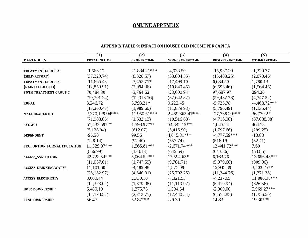
ONLINE APPENDIX
APPENDIX TABLE 9: IMPACT ON HOUSEHOLD INCOME PER CAPITA
(1) (2) (3) (4) (5) VARIABLES TOTAL INCOME CROP INCOME NON-CROP INCOME BUSINESS INCOME OTHER INCOME TREATMENT GROUP A -1,566.17 21,884.21*** -4,933.50 -16,937.20 -1,329.77 (SELF-REPORT) (37,329.74) (8,328.57) (33,804.55) (15,403.25) (2,070.46) TREATMENT GROUP B -11,665.43 -3,455.71* -17,499.10 6,634.50 1,780.13 (RAINFALL-BASED) (12,850.91) (2,094.36) (10,849.45) (6,593.46) (1,564.46) BOTH TREATMENT GROUP C 70,484.30 -3,764.62 -23,600.94 97,687.97 294.26 (70,701.24) (12,313.16) (32,642.82) (59,432.73) (4,747.52) RURAL 3,246.72 3,793.21* 9,222.45 -5,725.78 -4,468.72*** (13,260.48) (1,989.60) (11,879.93) (5,796.49) (1,135.44) MALE HEADED HH 2,370,129.94*** 11,950.61*** 2,489,663.41*** -77,768.20*** 36,770.27 (71,988.86) (1,632.13) (10,516.68) (4,716.98) (37,038.08) AVG AGE 57,433.59*** 1,598.97*** 54,342.19*** 1,045.24 464.78 (5,128.94) (612.07) (5,415.90) (1,797.66) (299.25) DEPENDENT -96.50 99.56 4,645.81*** -4,777.59*** -13.83 (728.14) (97.40) (557.74) (516.19) (52.41) PROPORTION_FORMAL EDUCATION 11,329.07*** 1,565.81*** -2,671.74*** 12,441.72*** 7.60 (866.99) (120.13) (645.59) (643.86) (63.85) ACCESS_SANITATION 42,722.54*** 5,064.52*** 17,594.63* 6,163.76 13,656.43*** (11,057.01) (1,747.59) (9,781.71) (5,079.66) (809.06) ACCESS_DRINKING WATER 17,101.60 -4,489.98 1,875.09 15,945.39 3,403.25** (28,182.97) (4,840.01) (25,702.25) (11,344.76) (1,371.38) ACCESS_ELECTRICITY 3,600.44 2,730.10 -7,321.53 -4,237.65 11,886.08*** (12,373.04) (1,879.08) (11,119.97) (5,419.94) (826.56) HOUSE OWNERSHIP 6,480.10 1,375.76 1,504.54 -2,000.06 5,969.27*** (14,178.52) (2,213.75) (12,440.34) (6,578.83) (1,336.50) LAND OWNERSHIP 56.47 52.87*** -29.30 14.83 19.30***

(37.49) (8.86) (31.01) (18.31) (3.14) CONSTANT -3898785.83*** -18,342.35 -3925239.35*** 898.32 -52,667.38 (151,241.77) (18,239.77) (134,173.44) (47,079.97) (39,908.79) OBSERVATIONS 12,242 12,222 12,232 12,242 12,242 R-SQUARED 0.19 0.12 0.12 0.21 0.05
Source: Author’s calculations. Note: Robust standard errors in parentheses *** p<0.01, ** p<0.05, * p<0.1.
APPENDIX TABLE 10: IMPACT ON HOUSEHOLD EXPENDITURE PER CAPITA
(1) (2) (3) (4) (5) (6) (7) (8) VARIABLES TOTAL EXP FOOD EXP NON-FOOD EXP CROP EXP NON-CROP EXP AGRI INPUT EXP EDU EXP HEALTH EXP TREATMENT GROUP A 19,801.55 -66.47 -2,326.36 2,171.13 5,506.69 9,650.88 2,922.63 2,067.18 (SELF-REPORT) (18,141.33) (489.80) (10,839.23) (2,263.55) (3,974.32) (7,286.28) (3,523.85) (1,430.33) TREATMENT GROUP B -14,742.40** -89.76 -6,897.35* -773.76 624.42 -6,963.83*** -752.76 164.74 (RAINFALL-BASED) (6,432.06) (153.68) (4,145.87) (930.07) (1,063.60) (2,598.86) (1,160.53) (323.03) BOTH TREATMENT GROUP C 10,980.94 -1,262.74 -14,489.95 181.87 1,460.01 20,035.51 1,641.43 3,364.20 (45,247.27) (886.03) (24,036.11) (6,207.58) (4,511.67) (21,969.91) (6,914.43) (3,867.18) RURAL -2,452.84 -168.16 -3,755.35 161.25 1,258.47 2,110.04 -2,505.46** 398.96 (5,785.10) (137.22) (3,666.77) (809.62) (846.07) (2,362.64) (1,053.31) (261.08) MALE HEADED HH 392,158.61*** 5,181.29*** 4,388.84 34,933.63*** 42,542.09*** 303,389.80*** -1,899.81* 2,957.70*** (18,834.92) (468.25) (10,216.43) (750.07) (680.68) (8,635.89) (1,073.62) (316.86) AVG AGE 29,019.50*** 672.97*** 11,163.26*** 2,139.41*** 3,972.81*** 13,070.56*** -1,252.66*** -307.28*** (2,439.89) (62.47) (1,411.58) (311.20) (259.86) (932.78) (300.55) (59.22) DEPENDENT -2,413.53*** -166.24*** -2,671.45*** -317.04*** 230.49*** 1,627.10*** -1,089.85*** 2.04 (342.55) (10.29) (181.03) (99.47) (44.42) (133.92) (52.98) (11.08) PROPORTION_FORMAL
EDUCATION 20,519.20*** 1,293.17*** 12,074.49*** 1,808.42*** 908.64*** 1,528.99*** 2,748.59*** 126.55***
(421.58) (12.64) (223.08) (123.96) (63.81) (162.28) (62.31) (12.21) ACCESS_SANITATION 17,254.61*** 120.84 6,741.45** 1,159.97 1,910.12** 6,891.03*** 739.16 -348.88 (5,193.54) (125.48) (3,317.89) (725.28) (792.02) (2,101.64) (933.49) (237.19)

ACCESS_DRINKING WATER 8,929.27 290.03 3,252.99 2,645.82 952.87 1,516.07 110.42 168.40 (13,160.49) (315.94) (8,207.08) (1,839.48) (2,357.65) (5,546.27) (2,547.87) (529.84) ACCESS_ELECTRICITY 8,376.70 379.86*** 8,777.07** 69.89 386.21 -1,837.47 209.57 323.73 (5,550.28) (133.43) (3,523.54) (762.92) (835.61) (2,275.84) (997.71) (262.85) HOUSE OWNERSHIP 919.13 -167.49 768.40 1,239.84 693.39 -661.25 -1,316.84 358.57 (6,574.19) (158.58) (4,175.91) (950.72) (958.34) (2,643.11) (1,257.96) (268.59) LAND OWNERSHIP 126.65*** 1.90*** 27.54** 20.55*** 11.41*** 56.40*** 9.25*** -0.46 (20.49) (0.46) (11.81) (3.29) (2.83) (9.64) (3.51) (0.72) CONSTANT -1114279.73*** -22,677.58*** -257,176.61*** -102,041.95*** -151,561.73*** -640,434.52*** 42,389.94*** 5,984.99*** (54,989.83) (1,386.18) (31,418.65) (8,324.48) (8,163.02) (23,707.98) (8,298.83) (1,786.27) OBSERVATIONS 12,242 12,242 12,242 12,222 12,232 12,242 12,242 12,242 R-SQUARED 0.63 0.92 0.52 0.36 0.25 0.31 0.27 0.04
Source: Author’s calculations. Note: Robust standard errors in parentheses *** p<0.01, ** p<0.05, * p<0.1.
APPENDIX TABLE 11: IMPACT ON TOTAL ASSET OUTCOMES
(1) (2) (3) VARIABLES ASSET STOCK AGRI INPUT ASSET VALUE DURABLE ASSET VALUE TREATMENT GROUP A -1,990.73 -15,691.41 -17,421.92 (SELF-REPORT) (33,184.36) (14,723.87) (88,561.35) TREATMENT GROUP B 4,475.63 -6,620.57 25,310.38 (RAINFALL-BASED) (12,235.93) (5,435.37) (30,435.15) BOTH TREATMENT GROUP C 11,009.94 -16,831.74 -154,958.27 (69,402.10) (21,241.71) (122,824.84) RURAL -19,365.10* -780.27 -57,247.53** (10,920.89) (5,112.05) (27,124.20) MALE HEADED HH -5,389.58 41,079.03*** 507,259.76*** (22,300.52) (3,770.74) (36,833.55) AVG AGE 25,045.10*** 4,321.08*** 41,710.50*** (4,168.51) (1,336.01) (8,558.51) DEPENDENT 5,188.91*** 2,938.38*** -6,594.53***

(791.12) (228.74) (1,578.76) PROPORTION_FORMAL EDUCATION -3,548.28*** -214.86 43,007.70*** (944.08) (276.79) (1,974.10) ACCESS_SANITATION 4,356.36 1,041.56 62,617.39*** (9,517.48) (4,789.09) (24,017.19) ACCESS_DRINKING WATER -37,269.07 3,304.72 -113,841.23 (28,588.08) (11,552.26) (72,146.55) ACCESS_ELECTRICITY -8,381.50 3,409.41 2,095.69 (10,063.28) (5,027.11) (25,979.66) HOUSE OWNERSHIP 9,091.28 11,804.14** -23,537.13 (12,448.63) (5,615.96) (31,454.58) LAND OWNERSHIP 36.87 41.86** 155.46 (46.59) (20.30) (104.25) CONSTANT -633,711.13*** -184,938.08*** -1197123.52*** (103,531.85) (36,826.19) (234,716.60) OBSERVATIONS 12,242 12,242 12,242 R-SQUARED 0.02 0.07 0.23
Source: Author’s calculations. Notes: a Robust standard errors in parentheses *** p<0.01, ** p<0.05, * p<0.1. b The variable ‘Asset Stock’ represents
total change in agricultural and other business asset in column 1.

APPENDIX TABLE 12: IMPACT ON LABOR MARKET OUTCOMES
(1) (2) (3) (4) (5) (6) VARIABLES MONTH PER YEAR_TOTAL DAYS PER
MONTH_TOTAL HOURS PER
DAY_TOTAL DAILY WAGE SALARIED WAGE YEARLY BENEFITS
TREATMENT GROUP A -1.03 -5.56 -1.60 -69.98 2,969.25 5,611.90 (SELF-REPORT) (5.50) (12.53) (4.02) (61.39) (2,771.30) (5,455.67) TREATMENT GROUP B 2.92 9.61** 1.74 26.60 -356.90 -2,381.25 (RAINFALL-BASED) (1.94) (4.53) (1.52) (22.82) (936.56) (1,954.30) BOTH TREATMENT
GROUP C -15.43 -16.51 -10.98 -77.83 -243.26 7,051.62
(9.39) (24.12) (7.63) (125.25) (6,422.49) (12,622.45) RURAL 2.17 6.65* 2.74** 21.61 -841.57 -1,613.85 (1.73) (3.98) (1.32) (20.06) (844.84) (1,739.93) MALE HEADED HH 79.92*** 235.07*** 92.90*** -1,546.64*** 40,315.81*** 108,490.36*** (6.75) (14.84) (4.18) (70.46) (1,840.75) (4,800.63) AVG AGE 9.78*** 21.73*** 5.95*** 30.07*** 2,802.27*** 5,881.37*** (0.88) (1.88) (0.54) (7.92) (272.36) (544.88) DEPENDENT 1.95*** 3.41*** 1.60*** 10.99*** 363.69*** 884.63*** (0.21) (0.48) (0.16) (1.33) (50.31) (87.46) PROPORTION_FORMAL
EDUCATION 8.24*** 19.62*** 6.16*** 38.48*** 1,015.94*** 974.11***
(0.26) (0.60) (0.19) (1.65) (61.63) (109.03) ACCESS_SANITATION -3.94** -5.72 -1.63 -42.37** -635.43 -3,849.87** (1.54) (3.50) (1.16) (17.95) (749.54) (1,543.41) ACCESS_DRINKING
WATER -4.13 -1.23 -1.52 -35.25 3,225.37* 3,529.74
(4.01) (9.26) (3.18) (45.52) (1,819.25) (3,817.83) ACCESS_ELECTRICITY 1.92 3.44 1.19 15.66 2,221.99*** 5,545.18*** (1.64) (3.74) (1.24) (19.20) (806.75) (1,656.76) HOUSE OWNERSHIP -4.60** -12.83*** -4.32*** 3.63 -2,859.47*** -3,352.70* (1.93) (4.47) (1.48) (22.71) (968.88) (1,964.48) LAND OWNERSHIP 0.01** 0.03** 0.01 -0.20*** 2.25 0.68 (0.01) (0.01) (0.00) (0.06) (2.61) (5.33)

CONSTANT -339.91*** -829.15*** -246.68*** 773.85*** -121,717.37*** -287,370.86*** (19.96) (44.49) (13.77) (183.22) (7,021.86) (14,980.65) OBSERVATIONS 12,242 12,242 12,242 12,242 12,242 12,242 R-SQUARED 0.87 0.87 0.87 0.54 0.35 0.21
Source: Author’s calculations. Note: Robust standard errors in parentheses *** p<0.01, ** p<0.05, * p<0.1.
APPENDIX TABLE 13: IMPACT ON HOUSEHOLD INCOME PER CAPITA (ROBUSTNESS CHECKS)
(1) (2) (3) (4) (5) VARIABLES TOTAL INCOME CROP INCOME NON-CROP INCOME BUSINESS INCOME OTHER INCOME
RAINFALL-BASED TREATMENT
GROUP -2,145.06 -937.98 -8,497.09* 4,267.58 2,035.72*
(4,802.50) (1,021.81) (4,532.01) (3,127.43) (1,042.35) RURAL 86.25 2,773.07* 5,713.50 -6,774.22* -4,021.64*** (6,992.38) (1,441.15) (7,032.28) (3,797.96) (897.11) MALE HEADED HH 106,440.79*** 4,264.46*** 156,608.46*** -5,018.54* -15,260.21*** (15,461.74) (496.82) (20,275.67) (2,910.94) (2,554.25) AVG AGE 1,229.56*** 124.30*** 1,347.41*** -306.14*** 350.77** (184.59) (25.64) (122.79) (75.28) (153.28) DEPENDENT -4,701.65*** -14.33 32.35 -4,688.90*** -90.49* (527.28) (88.56) (305.36) (465.09) (52.03) PROPORTION_FORMAL EDUCATION 16,755.88*** 1,690.66*** 2,690.49*** 12,332.62*** 109.99* (639.14) (116.50) (372.09) (577.51) (62.93) ACCESS_SANITATION 28,137.65*** 3,688.39*** 9,111.22 7,226.21** 12,450.55*** (5,844.87) (1,115.61) (5,635.89) (3,133.93) (670.22) ACCESS_DRINKING WATER 9,279.89 -2,129.37 3,819.89 9,384.62 1,355.08 (14,321.67) (3,043.71) (14,608.98) (7,128.38) (1,017.03) ACCESS_ELECTRICITY 8,673.53 2,563.74** -4,546.58 649.47 11,623.58*** (6,411.72) (1,181.42) (6,293.23) (3,337.99) (569.58) HOUSE OWNERSHIP 11,055.00 1,689.00 7,051.46 -2,355.96 3,424.35 (8,505.89) (1,953.56) (9,520.53) (4,902.26) (2,312.40)
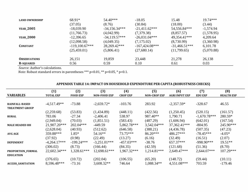
LAND OWNERSHIP 68.91* 54.40*** -18.05 15.48 19.74*** (37.05) (8.76) (30.84) (18.00) (3.44) YEAR_2005 -18,039.90 -34,156.34*** -21,411.62*** 54,556.84*** -1,574.94 (11,766.73) (4,042.99) (7,379.38) (8,857.57) (1,578.95) YEAR_2000 -12,396.65 -34,119.57*** -26,031.04*** 49,354.41*** 4,209.64 (12,098.58) (4,049.35) (7,175.02) (8,730.99) (3,360.98) CONSTANT -119,100.67*** 28,269.42*** -167,424.08*** -31,466.51*** 6,101.78 (25,459.01) (5,806.41) (27,680.14) (11,799.65) (5,070.88) OBSERVATIONS 26,151 19,859 23,448 21,278 26,138 R-SQUARED 0.56 0.59 0.10 0.61 0.03
Source: Author’s calculations. Note: Robust standard errors in parentheses *** p<0.01, ** p<0.05, * p<0.1.
APPENDIX TABLE 14: IMPACT ON HOUSEHOLD EXPENDITURE PER CAPITA (ROBUSTNESS CHECKS)
(1) (2) (3) (4) (5) (6) (7) (8) VARIABLES TOTAL EXP FOOD EXP NON-FOOD EXP CROP EXP NON-CROP EXP AGRI INPUT EXP EDU EXP HEALTH EXP
RAINFALL-BASED
TREATMENT GROUP -4,517.49** -73.88 -2,659.72* -103.76 283.92 -2,357.59* -328.67 46.55
(2,259.68) (53.83) (1,434.89) (448.11) (422.56) (1,250.45) (520.15) (161.57) RURAL 783.06 -27.34 -2,406.41 538.97 987.40** 1,790.71 -1,670.78*** 280.59* (2,949.04) (70.03) (1,851.51) (583.43) (487.29) (1,606.94) (642.01) (167.54) MALE HEADED HH 21,907.20*** 202.04*** -449.59 5,862.78*** 3,542.04*** 37,362.41*** -804.95 245.90*** (2,628.04) (40.93) (512.62) (646.58) (388.21) (4,436.78) (507.35) (47.23) AVG AGE 359.88*** 1.85* 54.16** 73.75*** 86.20*** 486.27*** -78.45*** -4.05* (37.92) (0.98) (22.49) (13.27) (6.16) (32.49) (16.51) (2.07) DEPENDENT -4,264.17*** -199.24*** -3,251.01*** -457.03*** -38.76 657.37*** -998.90*** 19.51** (306.02) (8.73) (166.44) (84.35) (42.59) (121.68) (51.36) (8.70) PROPORTION_FORMAL
EDUCATION 22,602.34*** 1,328.61*** 12,698.61*** 1,967.32*** 1,214.81*** 2,649.47*** 2,644.07*** 107.29***
(376.65) (10.72) (202.04) (106.55) (65.20) (148.72) (59.44) (10.11) ACCESS_SANITATION 8,596.48*** -73.16 3,608.32** 746.64 1,088.34** 4,551.08*** 703.59 -179.46

(2,643.09) (63.81) (1,671.99) (463.92) (439.50) (1,323.24) (567.36) (153.06) ACCESS_DRINKING WATER 4,638.76 72.97 1,421.14 1,550.78 653.52 1,686.38 65.63 160.70 (6,557.74) (158.38) (4,061.75) (1,164.35) (1,300.95) (3,465.29) (1,586.82) (358.96) ACCESS_ELECTRICITY 4,449.33 69.85 4,633.35*** 217.78 171.45 -663.59 475.94 249.72 (2,776.42) (66.83) (1,743.68) (481.47) (454.01) (1,420.08) (594.20) (165.28) HOUSE OWNERSHIP 4,199.54 -83.45 1,146.78 1,393.71* 1,095.40 1,342.54 -1,495.36* 214.66 (3,727.31) (90.01) (2,350.24) (837.30) (716.04) (2,210.73) (867.59) (190.43) LAND OWNERSHIP 128.02*** 1.80*** 27.49** 20.72*** 12.30*** 58.83*** 8.51** -0.38 (20.26) (0.45) (11.51) (3.28) (2.80) (9.74) (3.44) (0.71) YEAR_2005 -68,364.42*** -801.30*** -52,782.92*** 9,729.72*** -662.53 -12,265.40*** -2,071.87* -1,212.17*** (7,920.96) (202.30) (4,892.61) (1,111.50) (2,509.45) (3,092.95) (1,201.87) (338.89) YEAR_2000 -54,630.98*** -705.54*** -44,897.17*** 9,963.64*** 574.74 -12,097.30*** -1,600.02 -1,331.85*** (7,928.79) (202.65) (4,890.67) (1,115.94) (2,503.40) (3,078.71) (1,195.71) (344.68) CONSTANT 34,040.67*** 811.24*** 52,306.55*** -16,566.67*** -7,129.55** -37,782.12*** 9,344.28*** 739.84 (11,178.80) (274.00) (6,705.04) (1,753.38) (3,013.54) (6,836.29) (2,275.29) (492.02) OBSERVATIONS 26,155 26,155 26,141 19,859 23,448 20,750 21,219 20,034 R-SQUARED 0.94 0.99 0.92 0.77 0.72 0.75 0.74 0.26
Source: Author’s calculations. Note: Robust standard errors in parentheses *** p<0.01, ** p<0.05, * p<0.1.
APPENDIX TABLE 15: IMPACT ON TOTAL ASSET OUTCOMES (ROBUSTNESS CHECKS)
(1) (2) (3) VARIABLES ASSET STOCK AGRI INPUT ASSET VALUE DURABLE ASSET VALUE
RAINFALL-BASED TREATMENT
GROUP 3,629.59 -2,785.49 12,896.81
(5,539.19) (2,776.03) (10,480.90) RURAL -15,259.50** -187.89 -36,567.63*** (6,977.10) (3,681.45) (13,701.21) MALE HEADED HH 4,562.29*** 11,099.15*** 24,621.80*** (1,176.98) (1,055.20) (4,035.74)

AVG AGE 808.11*** 259.99*** 307.85** (88.38) (60.84) (136.93) DEPENDENT 3,575.13*** 2,623.12*** -8,969.50*** (855.46) (202.15) (1,583.03) PROPORTION_FORMAL
EDUCATION -1,726.24* 150.01 45,611.56***
(1,029.79) (248.05) (1,995.12) ACCESS_SANITATION 4,138.58 2,577.73 37,931.73*** (5,793.24) (3,192.82) (12,044.72) ACCESS_DRINKING WATER -23,286.11 3,115.43 -64,339.44* (17,949.09) (7,711.75) (35,597.94) ACCESS_ELECTRICITY -3,889.05 3,620.86 8,619.34 (6,058.37) (3,313.51) (12,880.07) HOUSE OWNERSHIP 8,248.68 11,351.01** -7,144.51 (9,264.73) (4,706.97) (17,672.48) LAND OWNERSHIP 41.75 42.90** 144.87 (45.89) (20.09) (102.02) YEAR_2005 5,980.47 20,747.40*** -301,520.67*** (10,034.68) (6,115.01) (30,942.39) YEAR_2000 5,402.68 18,363.10*** -259,561.93*** (10,123.89) (6,023.14) (31,214.49) CONSTANT -9,497.43 -47,858.02*** 343,272.54*** (22,196.07) (10,162.25) (50,634.36) OBSERVATIONS 21,278 19,448 26,070 R-SQUARED 0.06 0.29 0.77
Source: Author’s calculations. Notes: a Robust standard errors in parentheses *** p<0.01, ** p<0.05, * p<0.1. b The variable ‘Asset Stock’
represents total change in agricultural and other business asset in column 1.

APPENDIX TABLE 16: IMPACT ON TOTAL ASSET OUTCOMES (ROBUSTNESS CHECKS)
(1) (2) (3) VARIABLES ASSET STOCK AGRI INPUT ASSET VALUE DURABLE ASSET VALUE
RAINFALL-BASED TREATMENT
GROUP 12,208.38 2,793.33 -5,353.96
(9,256.13) (5,542.86) (15,512.84) RURAL -10,215.07 493.76 -44,680.72** (8,906.02) (4,694.77) (19,019.07) MALE HEADED HH 4,466.75*** 11,153.28*** 24,831.28*** (1,189.71) (1,047.33) (4,038.95) AVG AGE 807.29*** 257.33*** 300.77** (88.53) (60.74) (136.83) DEPENDENT 3,587.83*** 2,625.42*** -8,970.94*** (855.46) (202.30) (1,583.51) PROPORTION_FORMAL EDUCATION -1,721.82* 162.90 45,632.42*** (1,032.03) (247.83) (1,999.07) ACCESS_SANITATION 3,977.92 2,777.04 38,020.15*** (5,800.68) (3,202.50) (12,062.30) ACCESS_DRINKING WATER -23,031.97 3,099.31 -63,111.83* (17,940.62) (7,712.65) (35,516.49) ACCESS_ELECTRICITY -3,595.00 3,507.34 9,116.00 (6,032.44) (3,313.44) (12,857.04) HOUSE OWNERSHIP 8,155.81 11,314.44** -7,880.90 (9,278.08) (4,714.84) (17,700.17) LAND OWNERSHIP 11.95 44.60** 103.28 (42.58) (22.69) (105.35) INTERACTION_EDU*RAIN -104.33 -92.17 -102.15 (193.63) (87.10) (452.46) INTERACTION_LAND*RAIN 190.75 -13.78 310.37 (184.27) (41.67) (335.87) INTERACTION_RURAL*RAIN -14,849.04 -2,038.23 20,638.24 (11,637.86) (6,308.51) (21,450.97) YEAR_2005 6,844.60 18,588.25*** -298,447.12***
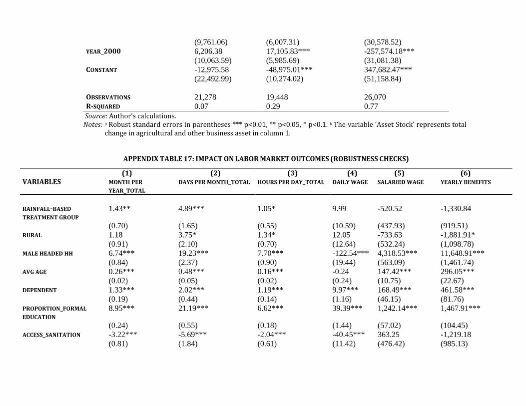
(9,761.06) (6,007.31) (30,578.52) YEAR_2000 6,206.38 17,105.83*** -257,574.18*** (10,063.59) (5,985.69) (31,081.38) CONSTANT -12,975.58 -48,975.01*** 347,682.47*** (22,492.99) (10,274.02) (51,158.84) OBSERVATIONS 21,278 19,448 26,070 R-SQUARED 0.07 0.29 0.77
Source: Author’s calculations. Notes: a Robust standard errors in parentheses *** p<0.01, ** p<0.05, * p<0.1. b The variable ‘Asset Stock’ represents total
change in agricultural and other business asset in column 1.
APPENDIX TABLE 17: IMPACT ON LABOR MARKET OUTCOMES (ROBUSTNESS CHECKS)
(1) (2) (3) (4) (5) (6) VARIABLES MONTH PER
YEAR_TOTAL DAYS PER MONTH_TOTAL HOURS PER DAY_TOTAL DAILY WAGE SALARIED WAGE YEARLY BENEFITS
RAINFALL-BASED
TREATMENT GROUP 1.43** 4.89*** 1.05* 9.99 -520.52 -1,330.84
(0.70) (1.65) (0.55) (10.59) (437.93) (919.51) RURAL 1.18 3.75* 1.34* 12.05 -733.63 -1,881.91* (0.91) (2.10) (0.70) (12.64) (532.24) (1,098.78) MALE HEADED HH 6.74*** 19.23*** 7.70*** -122.54*** 4,318.53*** 11,648.91*** (0.84) (2.37) (0.90) (19.44) (563.09) (1,461.74) AVG AGE 0.26*** 0.48*** 0.16*** -0.24 147.42*** 296.05*** (0.02) (0.05) (0.02) (0.24) (10.75) (22.67) DEPENDENT 1.33*** 2.02*** 1.19*** 9.97*** 168.49*** 461.58*** (0.19) (0.44) (0.14) (1.16) (46.15) (81.76) PROPORTION_FORMAL
EDUCATION 8.95*** 21.19*** 6.62*** 39.39*** 1,242.14*** 1,467.91***
(0.24) (0.55) (0.18) (1.44) (57.02) (104.45) ACCESS_SANITATION -3.22*** -5.69*** -2.04*** -40.45*** 363.25 -1,219.18 (0.81) (1.84) (0.61) (11.42) (476.42) (985.13)

ACCESS_DRINKING WATER -1.49 0.33 -0.82 -28.78 2,300.20** 2,830.52 (2.04) (4.70) (1.61) (28.50) (1,145.85) (2,408.82) ACCESS_ELECTRICITY 0.10 -0.66 -0.53 -5.50 2,236.07*** 4,817.54*** (0.85) (1.94) (0.64) (12.21) (512.13) (1,053.41) HOUSE OWNERSHIP -2.32** -6.63** -2.39*** 7.40 -2,244.74*** -3,067.48** (1.12) (2.60) (0.86) (14.68) (630.26) (1,308.89) LAND OWNERSHIP 0.02*** 0.03** 0.01* -0.19*** 2.39 1.87 (0.01) (0.01) (0.00) (0.06) (2.58) (5.26) YEAR_2005 11.88*** 36.08*** 2.98* 25.39 7,876.57*** 25,939.70*** (2.34) (5.25) (1.77) (25.59) (1,144.77) (2,177.14) YEAR_2000 15.46*** 45.70*** 5.55*** 23.66 7,896.82*** 25,232.90*** (2.37) (5.33) (1.79) (25.64) (1,146.71) (2,179.49) CONSTANT -13.43*** -42.90*** -5.36** 183.21*** -14,643.66*** -41,352.95*** (3.21) (7.43) (2.58) (44.66) (1,783.97) (3,687.19) OBSERVATIONS 25,499 25,499 25,499 20,731 20,731 20,731 R-SQUARED 0.98 0.98 0.98 0.89 0.77 0.56
Source: Author’s calculations. Note: Robust standard errors in parentheses *** p<0.01, ** p<0.05, * p<0.1.
APPENDIX TABLE 18: IMPACT ON LABOR MARKET OUTCOMES (ROBUSTNESS CHECKS)
(1) (2) (3) (4) (5) (6) VARIABLES MONTH PER
YEAR_TOTAL DAYS PER
MONTH_TOTAL HOURS PER
DAY_TOTAL DAILY WAGE SALARIED WAGE YEARLY BENEFITS
RAINFALL-BASED
TREATMENT GROUP 1.51 3.29 1.17 -20.65 -276.15 348.88
(1.03) (2.38) (0.79) (14.11) (605.78) (1,342.94) RURAL 1.05 3.25 1.19 -1.16 -608.69 -1,509.26 (1.24) (2.85) (0.94) (16.16) (679.61) (1,391.40) MALE HEADED HH 6.73*** 19.26*** 7.69*** -122.24*** 4,315.90*** 11,609.03*** (0.84) (2.37) (0.90) (19.42) (563.03) (1,461.07) AVG AGE 0.26*** 0.48*** 0.16*** -0.23 147.35*** 294.93***

(0.02) (0.05) (0.02) (0.24) (10.73) (22.62) DEPENDENT 1.32*** 2.02*** 1.19*** 9.94*** 169.02*** 464.56*** (0.19) (0.44) (0.14) (1.16) (46.17) (81.83) PROPORTION_FORMAL
EDUCATION 8.95*** 21.18*** 6.62*** 39.37*** 1,242.66*** 1,474.01***
(0.24) (0.55) (0.18) (1.44) (57.02) (104.57) ACCESS_SANITATION -3.20*** -5.72*** -2.02*** -40.11*** 359.53 -1,183.01 (0.81) (1.84) (0.61) (11.44) (477.67) (986.64) ACCESS_DRINKING WATER -1.53 0.33 -0.86 -28.93 2,323.15** 2,918.33 (2.04) (4.70) (1.61) (28.52) (1,145.75) (2,393.99) ACCESS_ELECTRICITY 0.08 -0.64 -0.55 -5.36 2,242.09*** 4,821.38*** (0.85) (1.94) (0.64) (12.22) (512.17) (1,055.25) HOUSE OWNERSHIP -2.31** -6.68** -2.38*** 6.58 -2,241.30*** -3,038.89** (1.13) (2.60) (0.86) (14.70) (631.32) (1,308.58) LAND OWNERSHIP 0.02*** 0.03** 0.01* -0.16** 1.17 -3.69 (0.01) (0.02) (0.00) (0.07) (2.82) (5.59) INTERACTION_EDU*RAIN -0.00 0.04 -0.01 0.27 -6.37 -55.31* (0.03) (0.07) (0.02) (0.34) (14.68) (29.58) INTERACTION_LAND*RAIN -0.01 -0.02 -0.01 -0.18 8.02 36.81** (0.02) (0.04) (0.01) (0.17) (6.95) (16.45) INTERACTION_RURAL*RAIN 0.32 1.33 0.37 39.41** -377.84 -1,158.47 (1.42) (3.29) (1.09) (19.55) (819.30) (1,752.70) YEAR_2005 11.73*** 36.43*** 2.81 28.18 7,884.11*** 25,537.27*** (2.32) (5.24) (1.77) (25.19) (1,127.28) (2,143.83) YEAR_2000 15.37*** 45.92*** 5.44*** 24.51 7,912.62*** 25,015.21*** (2.37) (5.34) (1.80) (25.47) (1,138.32) (2,167.19) CONSTANT -13.34*** -42.44*** -5.28** 192.92*** -14,758.39*** -41,868.88*** (3.26) (7.53) (2.61) (45.09) (1,803.41) (3,717.57) OBSERVATIONS 25,499 25,499 25,499 20,731 20,731 20,731 R-SQUARED 0.98 0.98 0.98 0.89 0.77 0.57
Source: Author’s calculations. Note: Robust standard errors in parentheses *** p<0.01, ** p<0.05, * p<0.1.
Related Documents


