. Distance-Based Phylogenetic Reconstruction ( part II ) Tutorial #11 © Ilan Gronau.

.

Distance-Based Phylogenetic

Reconstruction (part II)

Tutorial #11

© Ilan Gronau

.

Phylogenetic Reconstruction

We’d like to study the evolutionary history of species

.

Distance-Based Reconstruction

Given ML pairwise (evolutionary) distances between species,find the edge-weighted tree best describing this metric

The input: distance matrix – D– D(i,i) = 0– D(i,j) = D(j,i)– [ D(i,j) ≤ D(i,k) + D(k,j) ]

The Output: edge-weighted tree – T

• If D is additive, then DT = D

• Otherwise, return a tree best ‘fitting’ the input – D.

Note: Usually ML-estimated pairwise distances are not additive, but they are ‘close’ to some additive metric

metric

Bear Raccoon Weasel Seal Dog

Bear 0 26 34 29 32

Raccoon 26 0 42 44 48

Weasel 34 42 0 44 51

Seal 29 44 44 0 50

Dog 32 48 51 50 0

Bear

RaccoonWeasel

Seal

Dog

13

13

25.25

20

5.25

18.25

1.75

.

Neighbor-Joining Algorithms

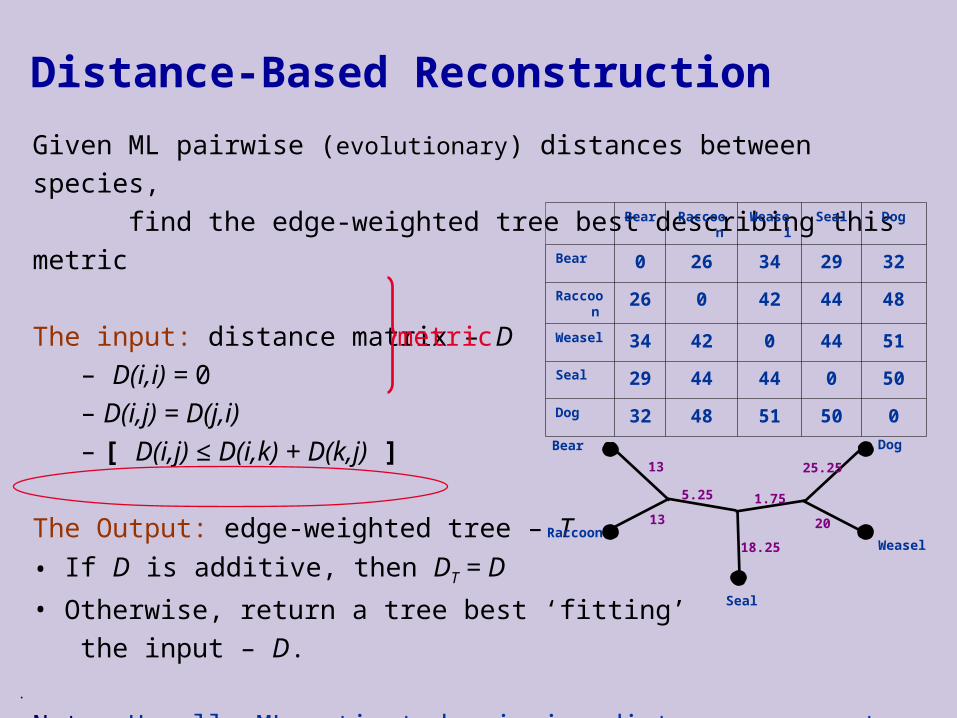
Agglomerative approach: (bottom-up)

1. Find a pair of taxa neighbors – i,j2. Connect them to a new internal vertex – v (Define edge

weights)3. Remove i,j from taxon-set, and add v (Define distances from

v)4. Return to (1)

When only 2 taxa are left, connect them

Consistency: Given an additive metric DT:

- We always choose a pair of neighbors in T (stage 1)

- The reduced distance-matrix is consistent with the reduced tree (stage 3)

Neighbors: taxa connectedby a 2-edge path

By induction:We eventually reconstruct T

.

UPGMA (Unweighted Pair Group Method with Arithmetic-Mean)

UPGMA algorithm:1. Find a pair of taxa of minimal distace– i,j2. Connect them to a new internal vertex v3. Remove i,j from taxon-set, and add v (D(v,k) = αD(i,k) +(1- α)D(j,k))4. Return to (1)

When only 2 taxa are left, connect them

Consistency ? - Given an additive metric DT, do we always choose a pair of neighbors in T ?

a b c d

a 0 14 15 27

b 0 3 15

c 0 14

d 0

c

13

1

13

1

1

a

b

d

UPGMA chooses b,c

Closest taxon is notnecessarily a neighbor

α, 1- α – proportional to the number of ‘original’ taxa i,j represent

.

Ultrametric Trees

• Edge-weighted trees which have a point (root) equidistant from all leaves

• Additive metrics consistent with an ultrametric tree are called ultrametrics

A distance-matrix is ultrametric iff it obeys the 3-point condition:“ Any subset of three taxa can be labelled i,j,k such that

d(i,j) ≤ d(j,k) = d(i,k) ”

66.5

3.5 4 32 2

3.5

tim

e

.

UPGMA

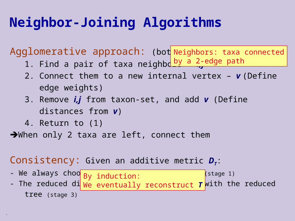
Additional notes:

• In the reduction formula D(v,k) can be set to any value within the interval defined by D(i,k) and D(j,k).

In particular: D(v,k) = ½(D(i,k) + D(j,k)) (WPGMA algorithm) If we use: D(v,k) = min {D(i,k) , D(j,k)} we get the ‘closest’

ultrametric from below (unique subdominant ultrametric)

Run-time analysis:― Naïve implementation: Θ(n3)― By keeping a sorted version of each row in D: Θ(n2log(n))― Third variant can be executed in: Θ(n2)

1. Find a pair of taxa of minimal distace– i,j

2. Connect them to a new internal vertex v

3. Remove i,j from taxon-set, and add v (D(v,k) = αD(i,k) +(1- α)D(j,k))

.

Consistent distance-based reconstruction:

Given an additive metric D, find the unique tree T, s.t. DT =

T. Reminder: A metric is additive iff it obeys the 4-point condition:

“Any subset of four taxa can be labelled i,j,k,l such that

d(i,j) + d(k,l) ≤ d(i,l) + d(j,k) = d(i,k) + d(j,l)”

Next Time …Distance matrices

Additive matrices

Ultrametric matrices

.

Saitou & Nei’s Neighbor Joining

S&N algorithm:1. Find a pair of taxa maximizing Q(i,j) = r(i) + r(j) – (n-2)D(i,j)

2. Connect them to a new internal vertex v with edges of weights:

3. Remove i,j from taxon-set, and add v - D(v,k) = ½(D(i,k) +D(j,k) -D(i,j))4. Return to (1)

When only 2 taxa are left, connect them (with edge of length D(i,j))

If D is additive (consistent with some tree T ):

•

• Q(i,j) is maximized for neighbor-pairs

• If i,j are neighbors then stages (2,3) are consistent

ik

kiDir ),()(

2

)()(),(

2

1),( ;

2

)()(),(

2

1(

n

irjrjiDvjw

n

jrirjiDi,v)w

jik

jipathkDjiDjiQ,

)),(,(),(2),( k

i j

v

n – current #taxa

shown in class

Conclusion: In such a case, given D, NJ returns T

.

Saitou & Nei’s Neighbor JoiningComplexity analysis

Run-time analysis:

• In each iteration we need to recalculate r(∙) for all taxa

• Q(∙,∙) values are ‘scrambled’ in each iteration

• Stage (1) takes O(n2)

• Total complexity - O(n3)

• No known way to speed this up significantly

ik

kiDir ),()(

2

)()(),(

2

1),( ;

2

)()(),(

2

1(

n

irjrjiDvjw

n

jrirjiDi,v)w

S&N algorithm:1. Find a pair of taxa maximizing Q(i,j) = r(i) + r(j) – (n-2)D(i,j)

2. Connect them to a new internal vertex v with edges of weights:

3. Remove i,j from taxon-set, and add v - D(v,k) = ½(D(i,k) +D(j,k) -D(i,j))

Note: There are consistent reconstruction algorithmswhich run in O(n2) or even O(n∙log(n)) time.

.

S&N’s NJ on Non-Additive Data

Example:

Bear Raccoon Weasel Seal Dog

Bear 0 26 34 29 32

Raccoon 26 0 42 44 48

Weasel 34 42 0 44 51

Seal 29 44 44 0 50

Dog 32 48 51 50 0

D:

D(B,R) + D(W,S) ; D(B,W) + D(R,S) ; D(B,S) + D(R,W)

26 + 44 (68) ; 34 + 44 (78) ; 29 + 42 (71)

D is not additive

.

S&N’s NJExample: 1st iteration

B R W S D

B 0 26 34 29 32R 0 42 44 48W 0 44 51S 0 50D 0

D:

Bear Dog Raccoon Weasel Seal

B-D

6 26

B R W S D

B 0 203 190 201 206R 0 205 195 197W 0 206 199S 0 198D 0

Q:

),(),(),(),(.3

2

)()(),(),(.2

),()(;),()2()()(),(.1

21

21

jiDkjDkiDkvD

n

jrirjiDviw

kiDirjiDnjrirjiQik

B R W S D

121 160 171 167 181r :

.

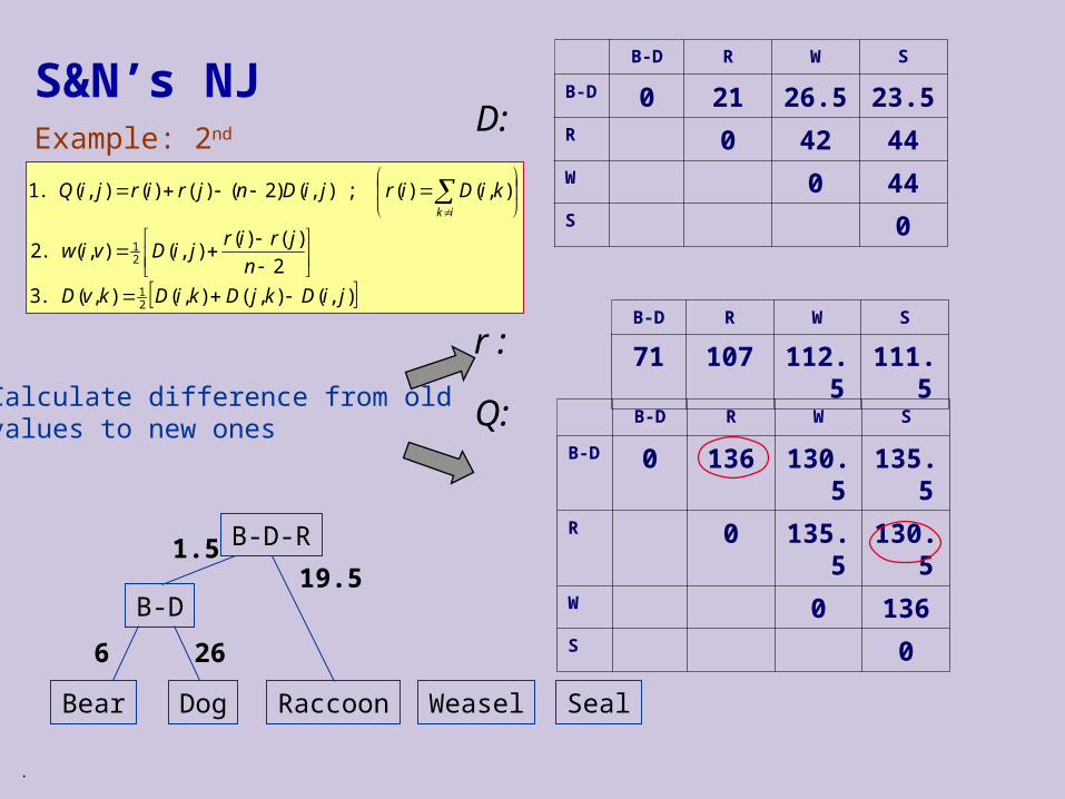
S&N’s NJExample: 2nd iteration

B-D R W S

B-D 0 21 26.5 23.5R 0 42 44W 0 44S 0

D:

Bear Dog Raccoon Weasel Seal

B-D

6 26

B-D R W S

B-D 0 136 130.5 135.5R 0 135.5 130.5W 0 136S 0

Q:

),(),(),(),(.3

2

)()(),(),(.2

),()(;),()2()()(),(.1

21

21

jiDkjDkiDkvD

n

jrirjiDviw

kiDirjiDnjrirjiQik

B-D R W S

71 107 112.5 111.5r :

B-D-R1.519.5

Calculate difference from oldvalues to new ones

.

S&N’s NJExample: 3rd iteration

B-D-R W S

B-D-R 0 23.75 23.25W 0 44S 0

D:

Bear Dog Raccoon Weasel Seal

B-D

6 26

Q:

),(),(),(),(.3

2

)()(),(),(.2

),()(;),()2()()(),(.1

21

21

jiDkjDkiDkvD

n

jrirjiDviw

kiDirjiDnjrirjiQik

B-D-R W S

47 67.75 67.25r :

B-D-R1.519.5

B-D-R W S

B-D-R 0 91 91W 0 91S 0

Reconstruct the uniquetree over 3 taxa

1.5

W-S

22.25 21.75

.

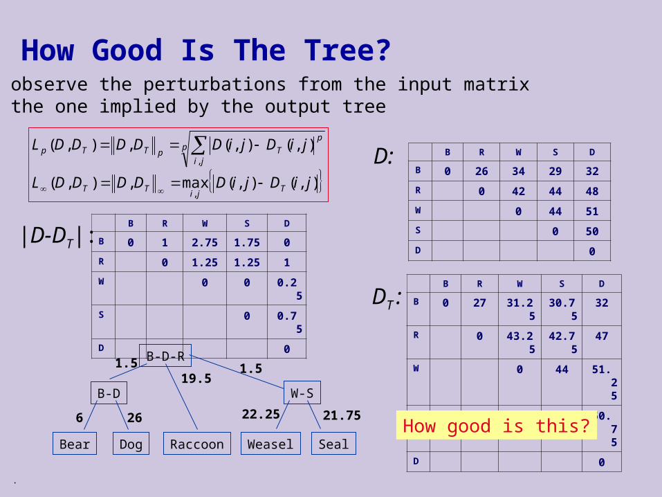
How Good Is The Tree?

Bear Dog Raccoon Weasel Seal

B-D

6 26

B-D-R1.519.5

1.5

W-S

22.25 21.75

We observe the perturbations from the input matrixto the one implied by the output tree

B R W S D

B 0 26 34 29 32

R 0 42 44 48

W 0 44 51

S 0 50

D 0

D:

B R W S D

B 0 27 31.25 30.75 32

R 0 43.25 42.75 47

W 0 44 51.25

S 0 50.75

D 0

DT :

),(),(max,),(

),(),(,),(

,

,

jiDjiDDDDDL

jiDjiDDDDDL

Tji

TT

p

ji

p

TpTTp

B R W S D

B 0 1 2.75 1.75 0

R 0 1.25 1.25 1

W 0 0 0.25

S 0 0.75

D 0

|D-DT|:

How good is this?

.

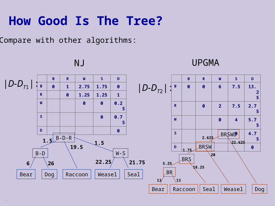
How Good Is The Tree?

Bear Dog Raccoon Weasel Seal

B-D

6 26

B-D-R1.519.5

1.5

W-S

22.25 21.75

Compare with other algorithms:

B R W S D

B 0 1 2.75 1.75 0

R 0 1.25 1.25 1

W 0 0 0.25

S 0 0.75

D 0

|D-DT2|:

Bear Raccoon WeaselSeal Dog

BR1313

BRS

18.255.25

BRSW20

1.75

BRSWD22.625

2.625

|D-DT1|:

NJ UPGMA

B R W S D

B 0 0 6 7.5 13.25

R 0 2 7.5 2.75

W 0 4 5.75

S 0 4.75

D 0

.

Can we do better?

Given a distance-matrix D, find an edge-weighted tree T,which minimizes ||D,DT||p

• For p = 1,2,∞ this task was shown to be NP-hard

• For p = 1,2 this task was shown to be NP-hard for ultrametric trees as well

• For p = ∞:― this task is easy (O(n2) algorithm) for ultrametric trees― 3-approximation algorithm for general trees

No algorithm which gives any good guarantees for non-additive data