© Crown copyright Met Office DIurnal cycle Coupling Experiment (DICE) GLASS / GASS joint project Martin Best and Adrian Lock presented by Ayrton Zadra

© Crown copyright Met Office DIurnal cycle Coupling Experiment (DICE) GLASS / GASS joint project Martin Best and Adrian Lock presented by Ayrton Zadra.
Dec 17, 2015
Welcome message from author
This document is posted to help you gain knowledge. Please leave a comment to let me know what you think about it! Share it to your friends and learn new things together.
Transcript
© Crown copyright Met Office
DIurnal cycle Coupling Experiment(DICE)
GLASS / GASS joint project
Martin Best and Adrian Lock presented by Ayrton Zadra

© Crown copyright Met Office Courtesy of Mike Ek

© Crown copyright Met Office
GLACE “hotspot” regions
Koster et al (2006)
• areas with significant coupling between precip and evaporation• derived from 12 GCM model which showed various coupling
strengths (bar graphs)• differences in coupling strength are not well known
GLACE = Global Land-Atmosphere Coupling Experiment

© Crown copyright Met Office
Outline of the 3 stages of DICE
LSM and SCM stand-alone performance against observations
What is the impact of coupling?
How sensitive are different LSM and SCM to variations in forcing?
SCM = Single Column ModelLSM = Land Surface Model
© Crown copyright Met Office
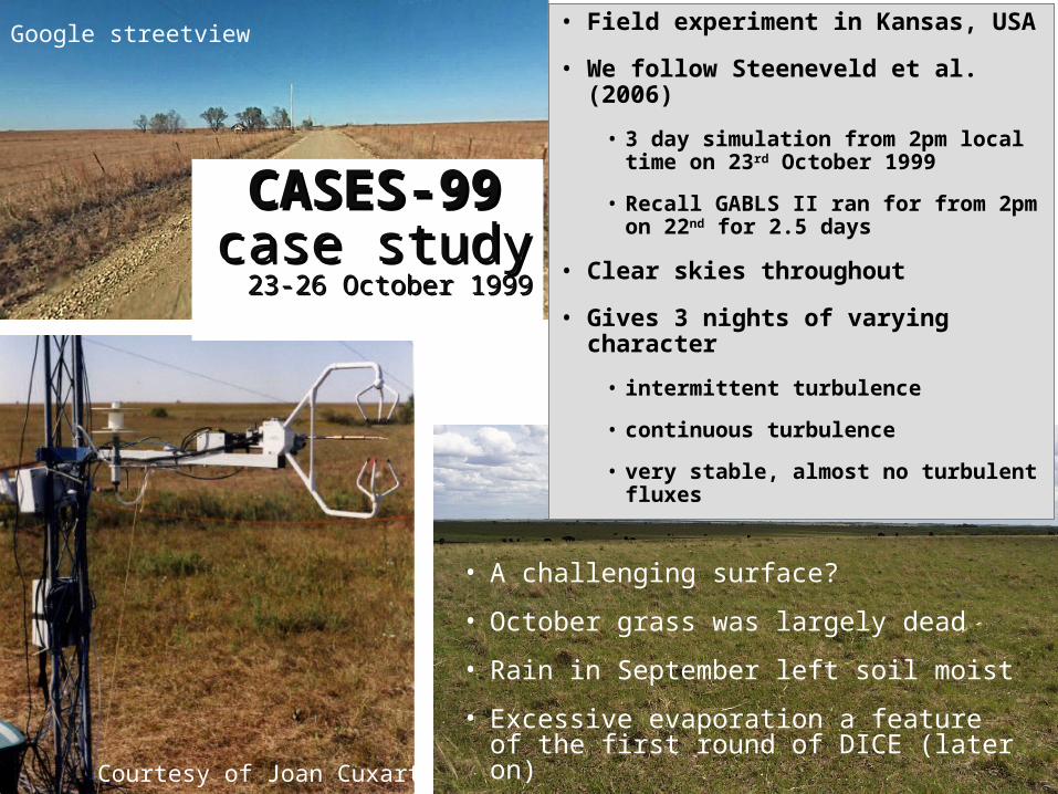
• A challenging surface?
• October grass was largely dead
• Rain in September left soil moist
• Excessive evaporation a feature of the first round of DICE (later on)
Google streetview
Courtesy of Joan Cuxart
CASES-99CASES-99 case studycase study
23-26 October 199923-26 October 1999
• Field experiment in Kansas, USA
• We follow Steeneveld et al. (2006)
• 3 day simulation from 2pm local time on 23rd October 1999
• Recall GABLS II ran for from 2pm on 22nd for 2.5 days
• Clear skies throughout
• Gives 3 nights of varying character
• intermittent turbulence
• continuous turbulence
• very stable, almost no turbulent fluxes

© Crown copyright Met Office
Experimental protocol
LSM •Soil spin-up:
• 9 years from saturated using WATCH forcing data
• 10th year forcing data from local site
•Two stage 1a experiments with forcing (obs) from 2m and 55m
•Stage 3a LSM experiments forced with stage 1b SCM data interpolated to 20
SCM
•Large-scale forcing:
• Time-varying geostrophic wind (uniform with height)
• Large-scale horizontal advective tendencies for T, q, u, v estimated from a simple budget analysis of the sondes
• Subsidence for T, q
• No relaxation
• Radiation switched on in all simulations
•SCM in stage 1b use observed sensible and latent heat fluxes and u* (either directly or via cD)
•Stage 3b SCM experiments forced with stage 1a LSM surface fluxes
© Crown copyright Met Office
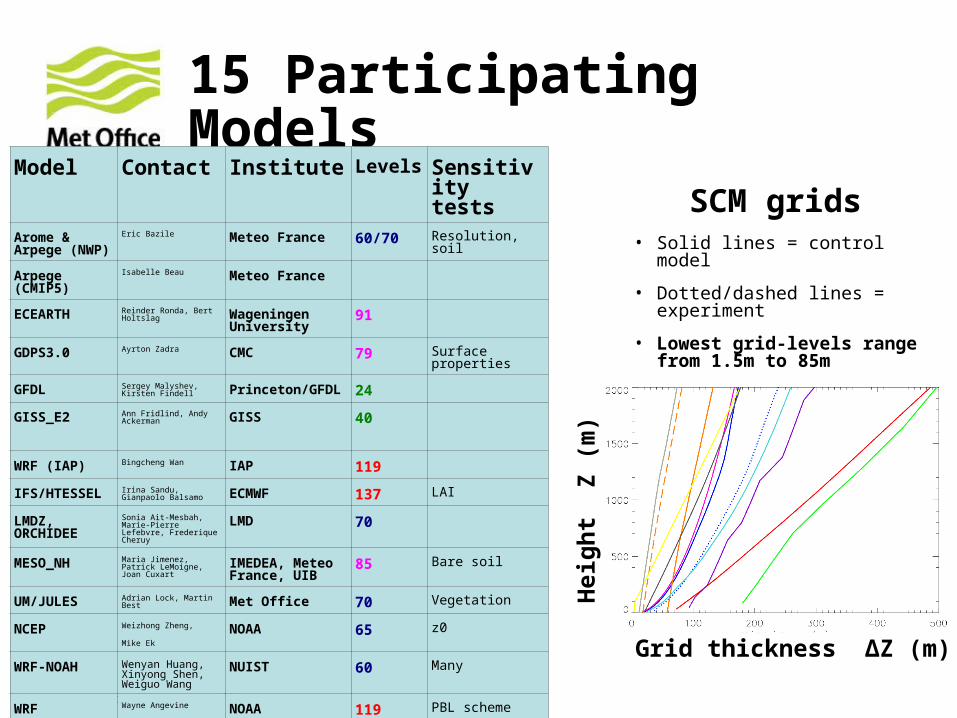
15 Participating Models
Model Contact Institute Levels Sensitivity tests
Arome & Arpege (NWP)
Eric Bazile Meteo France 60/70 Resolution, soil
Arpege (CMIP5) Isabelle Beau Meteo France
ECEARTH Reinder Ronda, Bert Holtslag Wageningen
University91
GDPS3.0 Ayrton Zadra CMC 79 Surface properties
GFDL Sergey Malyshev, Kirsten Findell Princeton/GFDL 24
GISS_E2 Ann Fridlind, Andy Ackerman GISS 40
WRF (IAP) Bingcheng Wan IAP 119
IFS/HTESSEL Irina Sandu, Gianpaolo Balsamo ECMWF 137 LAI
LMDZ, ORCHIDEE
Sonia Ait-Mesbah, Marie-Pierre Lefebvre, Frederique Cheruy
LMD 70
MESO_NH Maria Jimenez, Patrick LeMoigne, Joan Cuxart IMEDEA, Meteo
France, UIB85 Bare soil
UM/JULES Adrian Lock, Martin Best Met Office 70 Vegetation
NCEP Weizhong Zheng,
Mike Ek
NOAA 65 z0
WRF-NOAH Wenyan Huang, Xinyong Shen, Weiguo Wang
NUIST 60 Many
WRF Wayne Angevine NOAA 119 PBL scheme
CAM5, CLM4 David Lawrence, Ben Sanderson NCAR 26
SCM grids• Solid lines = control model
• Dotted/dashed lines = experiment
• Lowest grid-levels range from 1.5m to 85m
Grid thickness ΔZ (m)
Hei
gh
t Z
(m
)

© Crown copyright Met Office
Highlights fromstages 1 and 2

© Crown copyright Met Office
Stage 1aSurface fluxes from 55m-forced LSMs
Round 1 data
Round 2 data
Remember these will be the SCM surface fluxes in Stage 3b
Not all LSM provided u*(not compulsory under ALMA convention)
SHF
LHF
U*
Obs
© Crown copyright Met Office
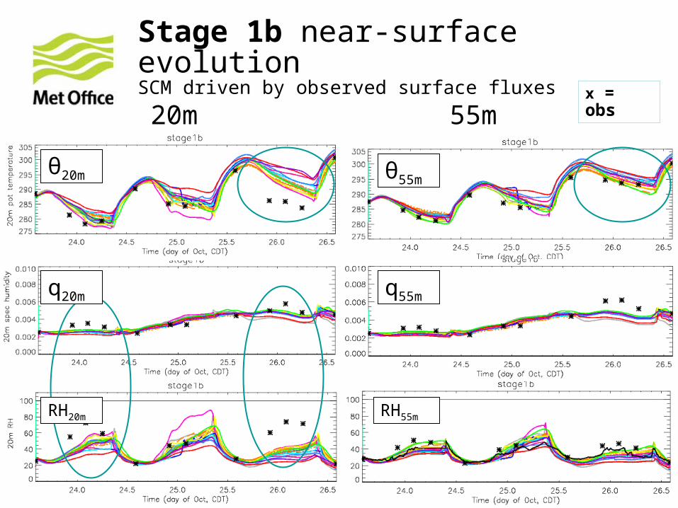
Stage 1b near-surface evolution SCM driven by observed surface fluxes
20m 55m
θ55mθ20m
q55m
RH55m
q20m
RH20m
x = obs

© Crown copyright Met Office
Stage 1b vs 2Bulk PBL sensitivity (variables at 55m)
• More spread between coupled models in stage 2 than stand-alone SCM in stage 1b
• More degrees of freedom• Moisture more sensitive than temperature?
θ55m
q55m
Stage 2
θ55m
q55m
Stage 1bx = obs

© Crown copyright Met Office
Stage 1b vs 2Bulk PBL depth (H) sensitivity• Some suggestion that PBL depth is less sensitive
when coupled (especially in the evening)
Stage 1b
Stage 2
PBL depth calculated as whereRiB=0.25
x = obs
H
H

© Crown copyright Met Office
Stage 1a vs 2Surface fluxes
• Similar surface fluxes from LSMs when coupled to their SCM, despite differences in atmospheric moisture
• to be confirmed from stage 3a
Selected stage 1a
wθ
wq
Stage 2
wθ
wq
--- obs

© Crown copyright Met Office
Stage 1a (55m)
Coupling and winds
x --- obs
u*
U @ 200m
U @ 200m
u* U @ 10m
Stage 1b
Stage 2
Stage 2
Stage 2

© Crown copyright Met Office
Stage 3aSurface flux sensitivities

© Crown copyright Met Office
Stage 3a – Qe (latent heat flux)
0 – CMC
1 – GFDL
2 – GISS
3 – IAP
4 – LMD
5 – NCEP
6 – NUIST
7 – SURFEX (default)
8 – SURFEX (root)
9 – WRF
10 – ECMWF (leaf)
11 – ECMWF (default)
12 – MetO
23rd 24th 25th
24th 25th
Nig
htD
ay

© Crown copyright Met Office
Stage 3a – Ustar (friction velocity)
0 – CMC
1 – GFDL
2 – GISS
3 – IAP
4 – LMD
5 – NCEP
6 – NUIST
7 – SURFEX (default)
8 – SURFEX (root)
9 – WRF
10 – ECMWF (leaf)
11 – ECMWF (default)
12 – MetO
23rd 24th 25th
24th 25th
Nig
htD
ay

© Crown copyright Met Office
Stage 3bDaytime sensitivities

© Crown copyright Met Office
Stage 3b daytime sensitivities
• All models have more variability in the PBL moisture than temperature
24th and 25th 24th and 25thθ300m q300m
SCM # SCM #

© Crown copyright Met Office
Stage 3b temperature sensitivity to SHF
Typically weak correlation between daytime PBL temperature and surface sensible heat flux
SHF
θ300m
24th
25th
© Crown copyright Met Office
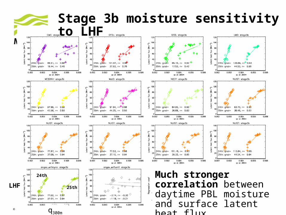
Stage 3b moisture sensitivity to LHF
Much stronger correlation between daytime PBL moisture and surface latent heat flux
LHF
q300m
24th
25th

© Crown copyright Met Office
Stage 3b sensitivities: PBL depth
• Some models have much greater sensitivity in PBL depth than others
24th and 25th
SCM #
PBL depth

© Crown copyright Met Office
Does PBL depth depend on surface buoyancy flux?
In most models, yes
H24th
25th
θv flux
© Crown copyright Met Office
Stage 3bNighttime sensitivities

© Crown copyright Met Office
Stable boundary layer
• As in daytime, more spread in moisture than temperature
23rd, 24th and 25th 23rd, 24th and 25th

© Crown copyright Met Office
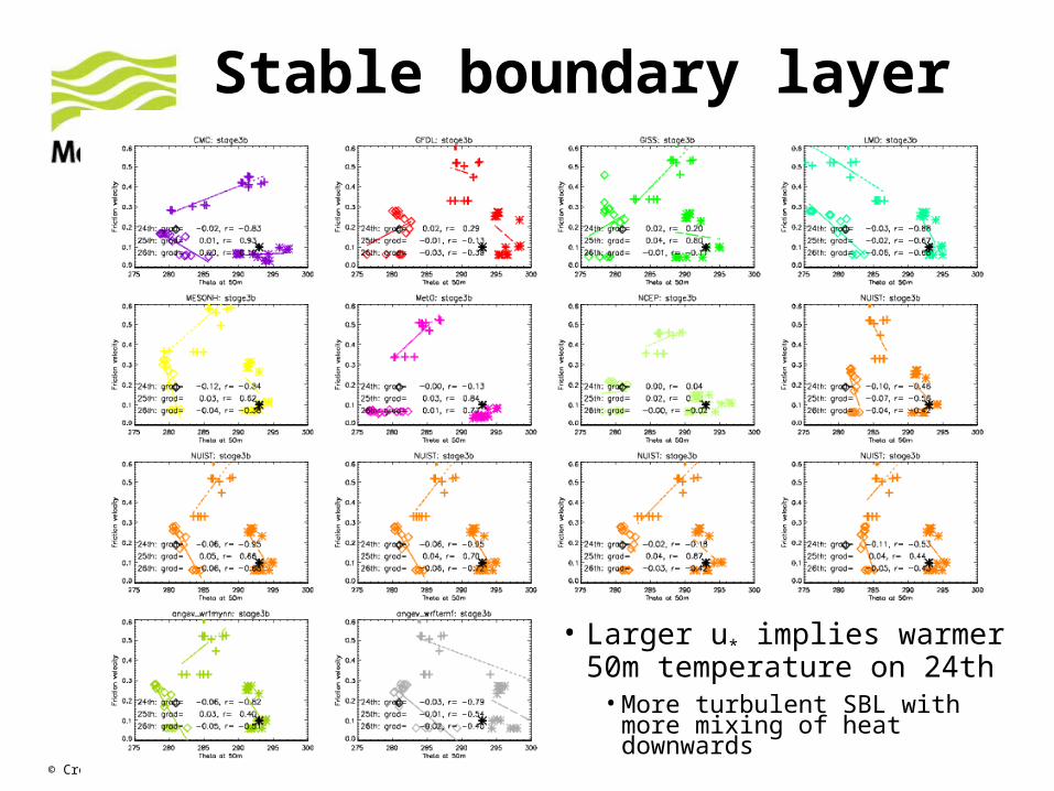
Stable boundary layer
• More negative SHF generally implies colder 50m temperature
• Heat lost to surface

© Crown copyright Met Office
Stable boundary layer
• Larger u* implies warmer 50m temperature on 24th
• More turbulent SBL with more mixing of heat downwards

© Crown copyright Met Office
DICE: summary so far
• Simple case (clear skies, no precipitation, homogeneous surface) but still a challenge for models
• Climatalogical vegetation in LSMs can lead to large errors in evaporation
• This dominated any signal of the impact of coupling in first round
• Second round those LSMs that needed to constrained evaporation (adjusting LAI, root depth, bare soil behaviour)
• Further discussion/developments are required to establish the best way to improve models
• Early results indicate interesting differences in different models’ sensitivity to changes in forcing that are likely to be important in GCMs and need to be understood
• Recent DICE discussions took place at the GEWEX conference, July 2014:
• Planned reruns: additional data from stage 1a, revised stage 3b forcing data
• Papers:
• Martin Best and Adrian Lock to write up intercomparison (overview paper plus two separate papers on LSM and SCM analyses, respectively)
• Special issue (eg BLM): to include participants' own analyses, model sensitivities, etc
More details at http://appconv.metoffice.com/dice/dice.html

© Crown copyright Met Office
Merci !
© Crown copyright Met Office
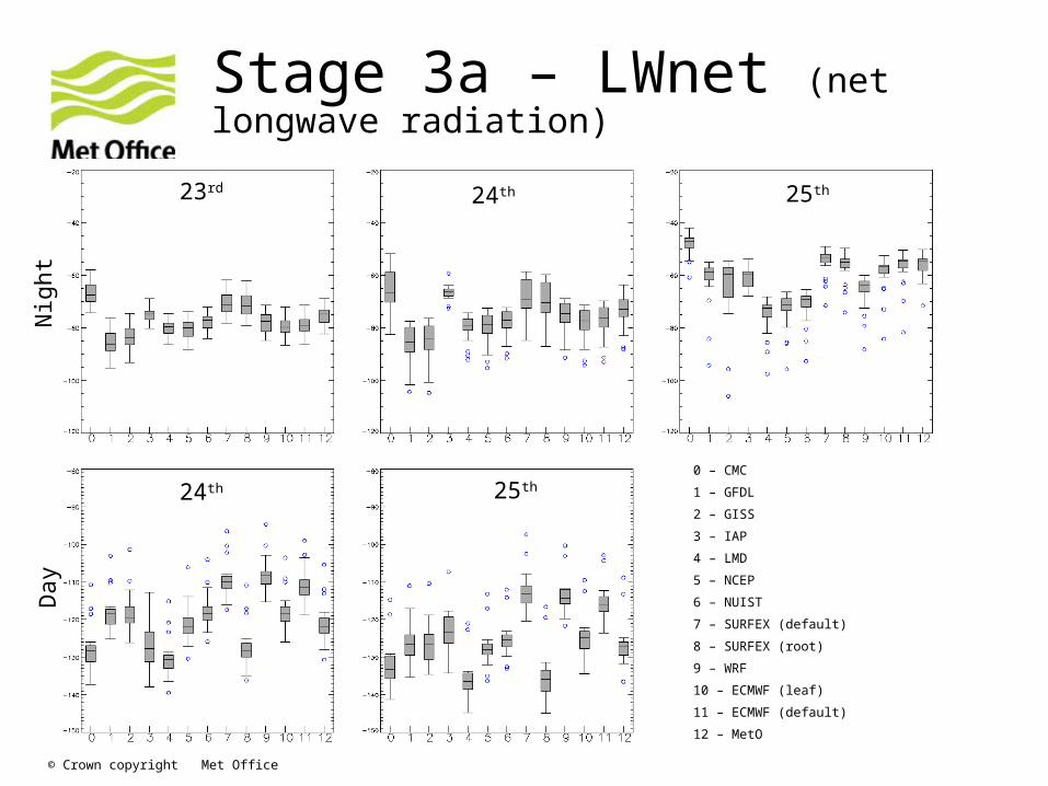
Stage 3a – LWnet (net longwave radiation)
0 – CMC
1 – GFDL
2 – GISS
3 – IAP
4 – LMD
5 – NCEP
6 – NUIST
7 – SURFEX (default)
8 – SURFEX (root)
9 – WRF
10 – ECMWF (leaf)
11 – ECMWF (default)
12 – MetO
23rd 24th 25th
24th 25th
Nig
htD
ay

© Crown copyright Met Office
Stage 3a – Qh (sensible heat flux)
0 – CMC
1 – GFDL
2 – GISS
3 – IAP
4 – LMD
5 – NCEP
6 – NUIST
7 – SURFEX (default)
8 – SURFEX (root)
9 – WRF
10 – ECMWF (leaf)
11 – ECMWF (default)
12 – MetO
23rd 24th 25th
24th 25th
Nig
htD
ay

© Crown copyright Met Office
Stage 3a – Qg (ground heat flux)
0 – CMC
1 – GFDL
2 – GISS
3 – IAP
4 – LMD
5 – NCEP
6 – NUIST
7 – SURFEX (default)
8 – SURFEX (root)
9 – WRF
10 – ECMWF (leaf)
11 – ECMWF (default)
12 – MetO
23rd 24th 25th
24th 25th
Nig
htD
ay

© Crown copyright Met Office
Daytime sensitivity: θ profiles
θ25th Oct 14:00 CDT14 SCMs

© Crown copyright Met Office
Daytime sensitivity: q profiles
q25th Oct 14:00 CDT14 SCMs
© Crown copyright Met Office
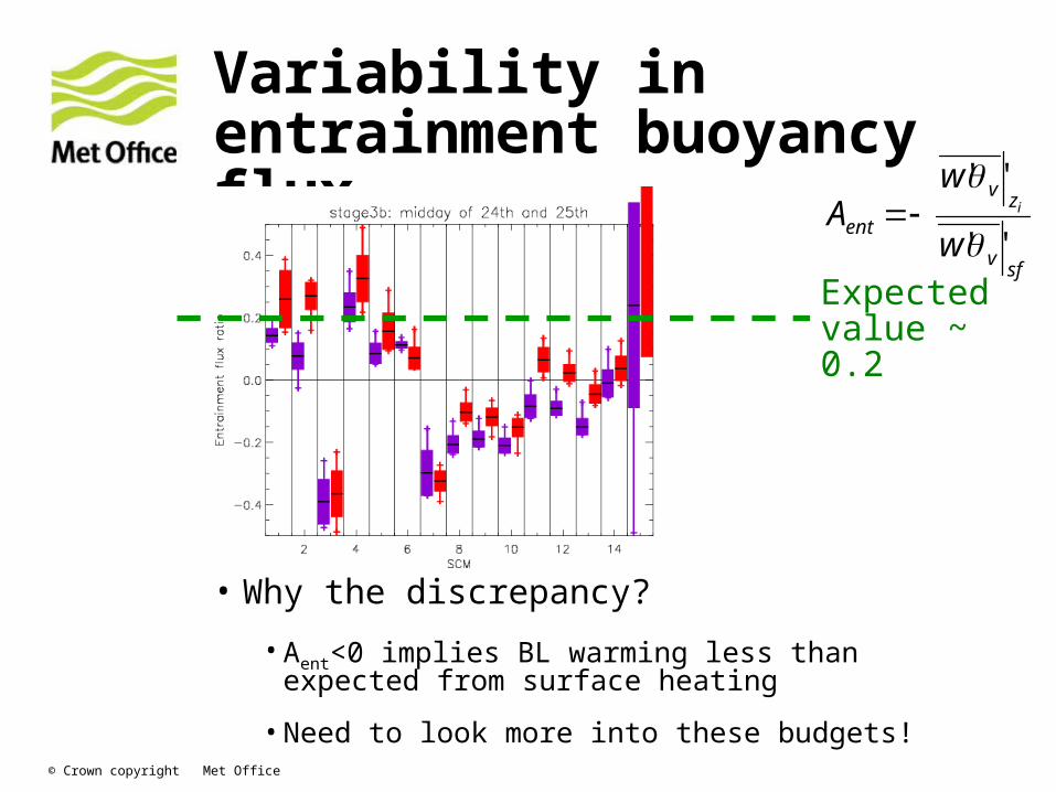
Variability in entrainment buoyancy flux
• Why the discrepancy?
• Aent<0 implies BL warming less than expected from surface heating
• Need to look more into these budgets!
Expected value ~ 0.2
sfv
zv
entw
wA i
''
''

© Crown copyright Met Office
Not really!
Does PBL depth depend on Evaporation Fraction?
H
EF
24th25th

© Crown copyright Met Office
Entrainment sensitivity
• Estimate entrainment fluxes from PBL θv budget
Average over the boundary layer:
Rearranging gives:v
i Sz
ww
t i
surfv
zv
v
''''
vS
z
w
tvv
''
1''''
''
v
i Stw
z
w
wA v
surfv
i
sfv
zv
ent
Horizontal advection and radiation (~small)• I’m ignoring vertical advection
© Crown copyright Met Office
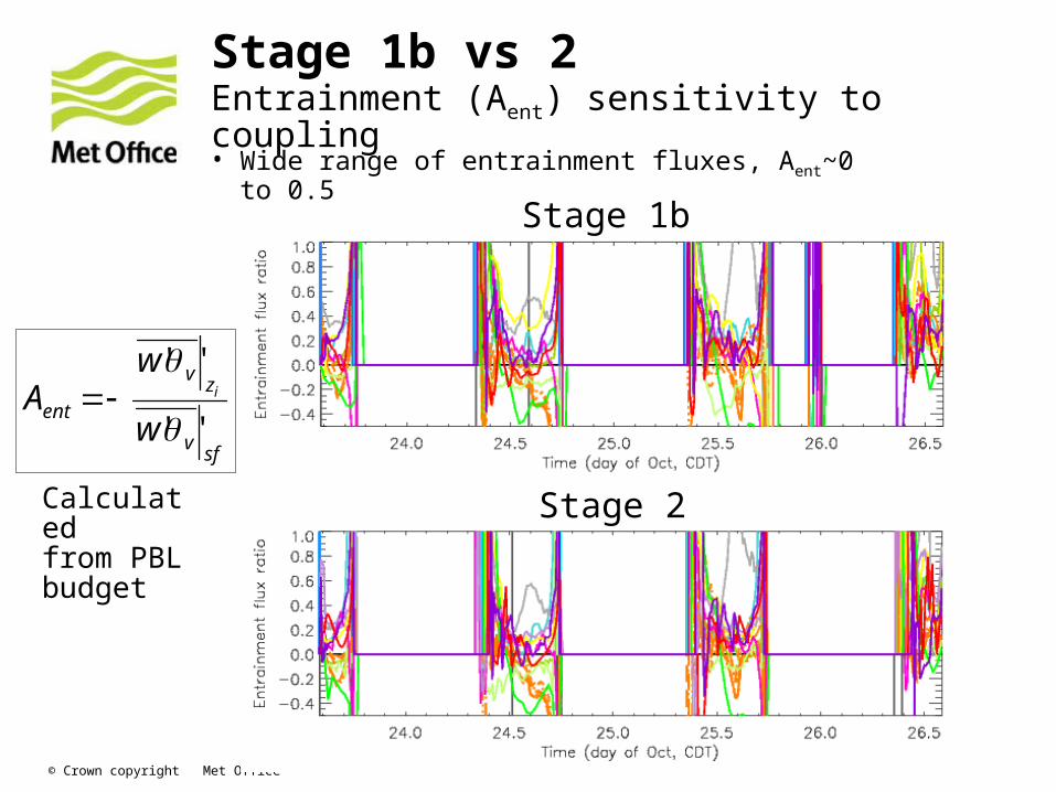
Stage 1b vs 2Entrainment (Aent) sensitivity to coupling
• Wide range of entrainment fluxes, Aent~0 to 0.5
Stage 1b
Stage 2
sfv
zv
entw
wA i
''
''
Calculated from PBL budget

© Crown copyright Met Office
Stable boundary layer
• More negative SHF generally implies colder 50m temperature
• Heat lost to surface
© Crown copyright Met Office
Stable boundary layer
• Larger u* implies warmer 50m temperature on 24th
• More turbulent SBL with more mixing of heat downwards
Related Documents