· Con ten ts In tro duction 1 1 Optimization 3 1.1 Basic Concepts. 3 1.2 Lo cal searc h. 4 1.3 Constrained Optimization. 6 1.3.1 Constrained optimization problem de ...

THE BALDWIN EFFECT AS AN OPTIMIZATION

STRATEGY Edgar Alfredo Dueñez Guzman and A. Hernández Aguirre

Comunicación Técnica No I-07-03/19-02-2007

(CC/CIMAT)

ContentsIntrodu tion 11 Optimization 31.1 Basi Con epts . . . . . . . . . . . . . . . . . . . . . . . . . . . . . . 31.2 Lo al sear h . . . . . . . . . . . . . . . . . . . . . . . . . . . . . . . . 41.3 Constrained Optimization . . . . . . . . . . . . . . . . . . . . . . . . 61.3.1 Constrained optimization problem denition . . . . . . . . . . 61.3.2 Te hniques to handle onstraints . . . . . . . . . . . . . . . . 61.3.2.1 Penalty fun tions . . . . . . . . . . . . . . . . . . . . 71.3.2.2 Rules of feasibility . . . . . . . . . . . . . . . . . . . 81.3.3 Sto hasti Ranking . . . . . . . . . . . . . . . . . . . . . . . . 101.3.3.1 Constraint handling . . . . . . . . . . . . . . . . . . 111.3.3.2 The Sto hasti ranking algorithm . . . . . . . . . . . 122 Evolutionary Algorithms 152.1 Denition of an Evolutionary Algorithm . . . . . . . . . . . . . . . . 152.2 Geneti Algorithms . . . . . . . . . . . . . . . . . . . . . . . . . . . . 172.2.1 The Simple Geneti Algorithm . . . . . . . . . . . . . . . . . . 182.2.2 More operators and odings . . . . . . . . . . . . . . . . . . . 192.3 Evolutionary Strategies . . . . . . . . . . . . . . . . . . . . . . . . . . 222.3.1 The ES(1 + 1) . . . . . . . . . . . . . . . . . . . . . . . . . . 232.3.2 ES(µ, λ) and ES(µ+ λ) . . . . . . . . . . . . . . . . . . . . . 242.3.3 More operators . . . . . . . . . . . . . . . . . . . . . . . . . . 252.3.4 A simple evolutionary strategy for onstrained optimization . 282.4 Memeti Algorithms . . . . . . . . . . . . . . . . . . . . . . . . . . . 292.4.1 Denition of a Meme . . . . . . . . . . . . . . . . . . . . . . . 292.4.1.1 Memes and Lamar kism . . . . . . . . . . . . . . . . 292.4.2 Denition of a memeti algorithm . . . . . . . . . . . . . . . . 292.5 Dierential Evolution . . . . . . . . . . . . . . . . . . . . . . . . . . . 302.5.1 The DE_1 algorithm . . . . . . . . . . . . . . . . . . . . . . . 312.5.2 The DE_2 algorithm . . . . . . . . . . . . . . . . . . . . . . . 322.5.3 More operators . . . . . . . . . . . . . . . . . . . . . . . . . . 322.5.4 Dierential evolution for onstrained optimization . . . . . . . 33iii

iv CONTENTS3 The Baldwin Ee t 353.1 Basi Con epts . . . . . . . . . . . . . . . . . . . . . . . . . . . . . . 363.1.1 Benets of phenotypi rigidity . . . . . . . . . . . . . . . . . . 363.1.2 Benets of phenotypi plasti ity . . . . . . . . . . . . . . . . . 373.1.3 Lamar kism and Baldwin Ee t . . . . . . . . . . . . . . . . . 373.1.4 The Darwinian me hanism . . . . . . . . . . . . . . . . . . . . 383.2 Baldwin Ee t and Computer S ien e . . . . . . . . . . . . . . . . . . 393.2.1 Hinton and Nowlan's experiment . . . . . . . . . . . . . . . . 423.2.1.1 Harvey's experiment . . . . . . . . . . . . . . . . . . 463.2.2 Turney's experiments . . . . . . . . . . . . . . . . . . . . . . . 463.2.2.1 Denition and types of bias . . . . . . . . . . . . . . 463.2.2.2 Shift of bias . . . . . . . . . . . . . . . . . . . . . . . 473.2.2.3 The Baldwinian model . . . . . . . . . . . . . . . . . 473.2.2.4 The algorithm . . . . . . . . . . . . . . . . . . . . . 483.2.2.5 Experiments . . . . . . . . . . . . . . . . . . . . . . 504 Baldwinian Optimization 574.1 The Learning Operator . . . . . . . . . . . . . . . . . . . . . . . . . . 584.2 Baldwinian Algorithms . . . . . . . . . . . . . . . . . . . . . . . . . . 604.2.1 Baldwinian evolutionary strategy . . . . . . . . . . . . . . . . 614.2.2 Baldwinian Dierential Evolution . . . . . . . . . . . . . . . . 684.3 Con lusions on the Experiments . . . . . . . . . . . . . . . . . . . . . 69Con lusions 77A Ben hmark fun tions 81B Results for the Mezura-Coello Ben hmark 93

List of Figures2.1 The s hemati view of the simple mutation operator. . . . . . . . . . 182.2 The s hemati view of the one-point rossover operator. . . . . . . . . 192.3 The s hemati view of the two-point rossover operator. Observe thatthe genotype is viewed as if it were a ring. . . . . . . . . . . . . . . . 202.4 The s hemati representation of the uniform rossover operator. Notethat at every rossover spot, the ospring has the genes of the se ondparent, while it has the genes of the rst elsewhere. . . . . . . . . . . 212.5 The s hemati view of the pseudo- rossover operator for dierentialevolution. We an observe that the rossed ve tor has 3 values of theoriginal ve tor, and 3 from the new one. . . . . . . . . . . . . . . . . 333.1 S hemati view of the tness lands ape for Hinton and Nowlan's sear hproblem. All genotypes have tness 0 ex ept for the orre t one withtness 1. . . . . . . . . . . . . . . . . . . . . . . . . . . . . . . . . . . 433.2 S hemati tness lands ape after learning.The sear h problem is smoother with a zone of in reased tness on-taining individual able to learn the orre t onne tion settings. . . . . 443.3 Relative frequen ies of 1's (dotted), 0's (dashed) and unde ided (solid)alleles in the population plotted over 50 generations. . . . . . . . . . 453.4 The average tness, bias strength, and bias orre tness of a populationof 1000 individuals, plotted for generations 1 to 10000, with three noiselevels. . . . . . . . . . . . . . . . . . . . . . . . . . . . . . . . . . . . 513.5 Experiment result for p = 0.5. The population is skewed towardsstronger bias. . . . . . . . . . . . . . . . . . . . . . . . . . . . . . . . 523.6 Bias strength xed at 0.75. . . . . . . . . . . . . . . . . . . . . . . . . 533.7 Bias strength xed at 0.5. . . . . . . . . . . . . . . . . . . . . . . . . 533.8 Bias strength xed at 0.25. . . . . . . . . . . . . . . . . . . . . . . . . 543.9 Bias strength in reases linearly from 0 in the rst generation to 1 inthe generation 5000. Afterwards, the bias is held onstant at 1. . . . 54v

vi LIST OF FIGURES4.1 S hemati representation of the Baldwinian implementation for learn-ing. The upper left individual is the original individual before learning.Then, at the upper right orner, the individual after learning with mod-ied tness and/or genotype. Finally, at the bottom, the individual asis to be ompared with other individuals. Observe that it retains itsoriginal genome, and only the tness is hanged. . . . . . . . . . . . . 58

List of Tables3.1 Reprodu tion of tradeos in evolution between phenotypi rigidity andphenotypi plasti ity [20 . . . . . . . . . . . . . . . . . . . . . . . . . 404.1 The known or reported optimum values for the test fun tions. The olumn max/min tells whether the problem is a maximization or aminimization to better interpret the results. . . . . . . . . . . . . . . 604.2 Results for fun tion g01 . . . . . . . . . . . . . . . . . . . . . . . . . 624.3 Results for fun tion g02 . . . . . . . . . . . . . . . . . . . . . . . . . 624.4 Results for fun tion g03 . . . . . . . . . . . . . . . . . . . . . . . . . 634.5 Results for fun tion g04 . . . . . . . . . . . . . . . . . . . . . . . . . 634.6 Results for fun tion g05 . . . . . . . . . . . . . . . . . . . . . . . . . 634.7 Results for fun tion g06 . . . . . . . . . . . . . . . . . . . . . . . . . 644.8 Results for fun tion g07 . . . . . . . . . . . . . . . . . . . . . . . . . 644.9 Results for fun tion g08 . . . . . . . . . . . . . . . . . . . . . . . . . 644.10 Results for fun tion g09 . . . . . . . . . . . . . . . . . . . . . . . . . 654.11 Results for fun tion g10 . . . . . . . . . . . . . . . . . . . . . . . . . 654.12 Results for fun tion g11 . . . . . . . . . . . . . . . . . . . . . . . . . 654.13 Results for fun tion g12 . . . . . . . . . . . . . . . . . . . . . . . . . 664.14 Results for fun tion g13 . . . . . . . . . . . . . . . . . . . . . . . . . 664.15 Results for fun tion i1 . . . . . . . . . . . . . . . . . . . . . . . . . . 664.16 Results for fun tion i2 . . . . . . . . . . . . . . . . . . . . . . . . . . 674.17 Results for fun tion i3 . . . . . . . . . . . . . . . . . . . . . . . . . . 674.18 Results for fun tion g01 . . . . . . . . . . . . . . . . . . . . . . . . . 694.19 Results for fun tion g02 . . . . . . . . . . . . . . . . . . . . . . . . . 704.20 Results for fun tion g03 . . . . . . . . . . . . . . . . . . . . . . . . . 704.21 Results for fun tion g04 . . . . . . . . . . . . . . . . . . . . . . . . . 704.22 Results for fun tion g05 . . . . . . . . . . . . . . . . . . . . . . . . . 714.23 Results for fun tion g06 . . . . . . . . . . . . . . . . . . . . . . . . . 714.24 Results for fun tion g07 . . . . . . . . . . . . . . . . . . . . . . . . . 714.25 Results for fun tion g08 . . . . . . . . . . . . . . . . . . . . . . . . . 724.26 Results for fun tion g09 . . . . . . . . . . . . . . . . . . . . . . . . . 724.27 Results for fun tion g10 . . . . . . . . . . . . . . . . . . . . . . . . . 724.28 Results for fun tion g11 . . . . . . . . . . . . . . . . . . . . . . . . . 73vii

viii LIST OF TABLES4.29 Results for fun tion g12 . . . . . . . . . . . . . . . . . . . . . . . . . 734.30 Results for fun tion g13 . . . . . . . . . . . . . . . . . . . . . . . . . 734.31 Results for fun tion i1 . . . . . . . . . . . . . . . . . . . . . . . . . . 744.32 Results for fun tion i2 . . . . . . . . . . . . . . . . . . . . . . . . . . 744.33 Results for fun tion i3 . . . . . . . . . . . . . . . . . . . . . . . . . . 74B.1 The known or reported optimum values for the rest of the test fun -tions. The olumn max/min tells whether the problem is a maximiza-tion or a minimization to better interpret the results. . . . . . . . . . 93B.2 Results for fun tion c01. The se ond and third olumn represent the omparison between the normal ES and the Baldwinian one, respe -tively. The fourth and fth is the omparison between the normal DEand the Baldwinian one respe tively. . . . . . . . . . . . . . . . . . . 94B.3 Results for fun tion c02. The se ond and third olumn represent the omparison between the normal ES and the Baldwinian one, respe -tively. The fourth and fth is the omparison between the normal DEand the Baldwinian one respe tively. . . . . . . . . . . . . . . . . . . 94B.4 Results for fun tion c03. The se ond and third olumn represent the omparison between the normal ES and the Baldwinian one, respe -tively. The fourth and fth is the omparison between the normal DEand the Baldwinian one respe tively. . . . . . . . . . . . . . . . . . . 94B.5 Results for fun tion c04. The se ond and third olumn represent the omparison between the normal ES and the Baldwinian one, respe -tively. The fourth and fth is the omparison between the normal DEand the Baldwinian one respe tively. . . . . . . . . . . . . . . . . . . 95B.6 Results for fun tion c05. The se ond and third olumn represent the omparison between the normal ES and the Baldwinian one, respe -tively. The fourth and fth is the omparison between the normal DEand the Baldwinian one respe tively. . . . . . . . . . . . . . . . . . . 95B.7 Results for fun tion c06. The se ond and third olumn represent the omparison between the normal ES and the Baldwinian one, respe -tively. The fourth and fth is the omparison between the normal DEand the Baldwinian one respe tively. . . . . . . . . . . . . . . . . . . 95B.8 Results for fun tion c07. The se ond and third olumn represent the omparison between the normal ES and the Baldwinian one, respe -tively. The fourth and fth is the omparison between the normal DEand the Baldwinian one respe tively. . . . . . . . . . . . . . . . . . . 96B.9 Results for fun tion c08. The se ond and third olumn represent the omparison between the normal ES and the Baldwinian one, respe -tively. The fourth and fth is the omparison between the normal DEand the Baldwinian one respe tively. . . . . . . . . . . . . . . . . . . 96

Dedi atoryThis thesis is dedi ated to three broad groups of people.To my family for their support sin e the early stages of my life to present andfuture. Spe ially to my wife Claudia be ause if it were not by her I would have neverdone my Masters of S ien e. To my parents Margarita and Ernesto for the un ondi-tional help they have always given me, and the impe able formation I re eived fromthem. To my brothers Ernesto and Eduardo who made my life mu h better, ea h onein his very spe ial and omplementary way.To my friends, who are as a se ond family to me, and who always were therewhen I was parti ularly down. To the Plano as a ommunity, but very spe ially toBeta, Carlos, Eugenio, Inder, Limolín, Marte, Pon hito, Raúl, Saúl and Veróni a (instri tly alphabeti al order) for making my years in Guanajuato the happiest of mylife.To my professors, who build my temper and knowledge in a way I never thoughtpossible. I will not mention anyone sin e I would surely omit very important people.My gratitude to them all.

ix

x LIST OF TABLES

A knowledgmentsI would like to thank Arturo Hernández Aguirre, my thesis advisor, for believing inme and helping me to nish my degree. Also, thanks to Mariano Rivera and JohanVan Horebeek for being a orner-stone in my late Ba helor's and early Masters' years.Very spe ially, I want to thank the ommunity CIMAT-FAMAT for being a shelterof knowledge and formation. They believed in me and allowed many a tivities on mybehalf, always supporting and helpful.

xi

xii LIST OF TABLES

Introdu tionBiologi ally inspired models in omputer s ien e used for problem solving have re-sulted invaluable to the ommunity. It has been almost half a entury sin e therst attempt were made towards su essful appli ations of these models to real worldproblems.A model is by denition a simpli ation of reality, and it is usually the ase that it an end in over-simpli ation of observed phenomenon. In evolutionary omputationthis might be the ase sin e, from the point of view of biology, neo-Darwinism is amore omplex model than any urrent evolutionary algorithm. This is also the asein many biologi ally inspired models as arti ial neural networks, ma hine learning,automata theory, and more.Making more and more omplex models seems to be a trend of hanging strength.While some resear hers like more sophisti ated methods for problem solving, otherssuggest that we should be trying to dis over the inners of the urrent algorithms inorder to set them on more formal foundations.The main aim of this thesis is to present a biologi ally inspired, and to someextent, biologi ally a urate new trend in evolutionary omputation by expresselytrying to emulate the observed behavior known as the Baldwin Ee t.A number of resear hers have observed (in both, evolutionary omputation andevolutionary biology) a synergy between learning and evolution to a ertain extent.This synergy is ommonly (and mistakenly) known as the Baldwin Ee t. While itis true that the Baldwin Ee t explains this observed synergy, it is equally interestedwith the osts of learning over instin t. Con erning learning and instin t as a pe u-liar duality, the Baldwin Ee t an be thought as the synergy, osts and trade-oso urring between them.Some experiments have been made by a handful of resear hers, a quainted tosome degree with both biology and omputation, to study the Baldwin Ee t inits omplete form. The results were promising and inspired the author in furtherstudying this phenomenon.This thesis is organized as follows:In the rst Chapter we give a brief introdu tion to Optimization without wantingto make it the entral point. The key terms are explored and an introdu tion tolo al sear h and onstrained optimization will be given. These on epts will be usedthroughout the thesis, and it is re ommended that the reader at least ips thoughthem to be sure to understand the notation adopted and get used with names of1

2 LIST OF TABLESalready known terms.The se ond Chapter is devoted to evolutionary algorithms. There, we develop thebasi denitions and algorithms. There is no attention given to results on erningproofs of onvergen e rate or underlying me hanisms for the algorithms, instead wetry to develop the reader's intuition on the required steps to reate and understandan evolutionary algorithm. Some of the main bran hes of this eld are inspe ted,and a number of variants are dis ussed. The notions of evolutionary strategies anddierential evolution will be the key for the presented experiments, and should begiven spe ial onsideration.In the next Chapter, we dis uss about the Baldwin Ee t. We are on entrated ona detailed explanation of the on epts and trends in this matter. We present the workof several other resear hers in order to support our remarks, and give spe ial attentionto the Baldwin Ee t as a whole. After developing the Baldwinian and Lamar kism on epts, we ontinue with a Se tion devoted to Baldwin Ee t in omputer s ien e.There we present the more traditional works in this eld, and give explanations ofthe observed behaviors.The last Chapter is then lled with the entral portion of this thesis. We presentthe term Baldwinian Optimization, whi h to the extent of our knowledge has neverbeen used before. There we express the viability of using Baldwinian me hanisms tosolve di ult onstrained optimization problems, and also give the key ideas on howto adapt a Baldwinian version of virtually any population based algorithm. We alsopresent a omparison between Baldwinian and non-Baldwinian versions of the samealgorithm, and lose with a small on lusion on the results obtained.The on lusions on the work presented follow these Chapters. There we argueabout the possibilities of the Baldwinian optimization as a resear h resour e. Webriey argue that biologi ally inspired algorithms are more easily understood andadapted on the long run than other, more obs ure, ones.

Chapter 1OptimizationThe body of mathemati al results and numeri al methods for nding and identify-ing the best andidate from a olle tion of alternatives without having to expli itlyenumerate all possible alternatives is alled Optimization. With the advent of theinformation era, the omputational power have made the optimization task easier,but at the same time have brought a new range of questions on erning the e ien yand orre tness of the algorithms used in optimization.In this Chapter we provide the basis for global and onstrained optimization. Theaims of this Chapter are to develop the required denitions and to present a range ofgeneral-purpose te hniques to atta k an optimization problem.1.1 Basi Con eptsThe general optimization problem an be stated as follows. Given the pair (S; f),where S is an arbitrary sear h spa e, and f : S → R is a real-valued fun tion tooptimize. With the optimum of the problem, we mean either the maximum of thefun tion or the minimum.For purposes of this thesis, the optimization problem will always be regarded as amaximization problem. Observe that every minimization problem an be transformedinto a maximization one by simply taking the problem as (S;−f).The value x∗ is alled the optimum (maximum) of the optimization problem (S; f)if and only if it satises f(x∗) ≥ f(x) for every x ∈ S. When if along with the sear hspa e we have a neighboring stru ture N : S → 2S dened on it, we an denethe notion of lo al optimum as every value x∗local satisfying f(x∗local) ≥ f(x) for everyx ∈ N(x∗local). By notation we will dene X∗ = x|x is an optimal solution of (S; f),and X∗

local = x|x is a lo al optimal solution of (S,N ; f).Observe that the denition of a lo al optimum is dependent on the neighboringstru ture asso iated to the sear h spa e. With the appropriate neighboring stru ture,we an avoid lo al optimum solutions that are not global ones. We an also note thatX∗ ⊂ X∗

local regardless of the neighboring stru ture N .In general, we will have that S ⊂ Rm, for ontinuous optimization, and S ⊂ Nm,3

4 CHAPTER 1. OPTIMIZATIONfor dis rete optimization. We will all the elements x ∈ S solutions of the optimizationproblem, as they represent the possible solution values of an optimization problem.Similarly, we will all f(x), for x ∈ S, the values of a solution. By notation, f(x∗)will be alled the optimum value of the optimization problem.In general, we an only tell if we are at a lo al optimum or not, sin e the notionof lo al optimum is based on a neighboring stru ture that is potentially very small ompared to the size of the sear h spa e S. In order to be sure that we are in theglobal optimum, we have to enumerate all possible solutions and he k if all of themare not greater than our proposed solution.We also require a little more from the neighboring stru ture, as not every stru tureis useful. Given an optimization problem (S,N ; f), the neighboring stru ture is saidto be onsistent if for every pair of solutions x, y ∈ S, there exists a sequen e (notne essarily nite) zii∈Z, su h that x = limi→−∞ zi and y = limi→∞ zi, and zi+1 ∈N(zi) for every i ∈ Z. If the sequen e is nite, N is said to be nitely onsistent.This denition denes whether a neighboring stru ture an lead from one point inthe sear h spa e to every other passing only through the neighbors (and the neighborsof the neighbors) of the points to be united. Observe that if S is nite, then every Nis nitely onsistent.Let us now dene a relation for neighboring. Given the relation ∼⊂ S × S, su hthat x ∼ y if and only if x ∈ N(y), we an dene ertain desirable properties of theneighboring stru ture N . We will say that N is oherent, if and only if ∼ is reexive(i.e. x ∼ x) and symmetri (i.e. x ∼ y ⇔ y ∼ x).The notion of onsisten y is used by many sto hasti lo al sear h algorithms toassert global optimality, while the notion of oheren y is mainly used for onvenien e.There is also another denition that will prove useful in our study. We will saythat the fun tion f is unimodal in T ⊂ S if and only if X∗

local of the redu ed problem(T,N |T , f) has ardinality 1 (in other words, if there is only one lo al optimum in T )If the fun tion f is not unimodal in T , then it is said to be multi-modal.1.2 Lo al sear hThe rst type of algorithms we might nd in optimization history are the lo al sear halgorithms. This early attempt to solve optimization problems an be regarded as afun tion

a : S → 2S where a(x) ∈ N(x) for ea h x ∈ S (1.1)The algorithm an be either deterministi (i.e. a fun tion as proposed above) orsto hasti in whi h ase we an generalize the above denition to bea : S × [0, 1] → 2S where a(x, r) ∈ N(x) for ea h x ∈ S, r ∈ [0, 1] (1.2)where the number r is onsidered to be the random portion of the algorithm.The pseudo- ode for the lo al sear h algorithm is given below to express the wayin whi h the lo al sear h algorithm work.

1.2. LOCAL SEARCH 5Lo al sear h (sto hasti )i =initialSolution();best =i;iterations = 0;while( depth-not-satisfied )

count = 0;// Here starts the algorithm a.while( pivot-rule-not-satisfied )j =next( N(i) );count+ +;if( f(j) > f(best) )

best = j;// We think of best as the produ tion//of the algorithm best = a(i)i = best;iterations + +;In this pseudo- ode we an observe a ouple of onditions, the depth ondition andthe pivot rule. This pair of onditions determine the lo al sear h algorithm.The pivot rule is the algorithm itself, and an be for instan e steepest as ent,meaning that the whole neighborhood of the solution i is to be sear hed for the bestsolution available (count = |N(i)|). In the ase of greedy as ent, we might use thepivot rule of stopping when the rst better solution in the neighborhood is found(count = |N(i)| or best = i). In pra ti e, as the ardinality of the neighborhood N(i) an be innite, it is natural to onsider only a random sample of size n ≪ |N(i)|.This type of algorithms are deterministi in nature, but sto hasti in behavior.The depth ondition is the termination riteria of the lo al sear h. It an rangefrom the one-time lo al sear h (when iterations = 1), to the lo al optimality ondition(count = |N(i)| and best = i).Another important remark is that sto hasti lo al sear h algorithms will have anon-deterministi pivot rule. This means that they might a ept a solution generatedwithin the neighborhood based on a probabilisti ondition. Algorithms like simulatedannealing fall into this ategory, where a worst solution might be a epted with lowprobability.

6 CHAPTER 1. OPTIMIZATION1.3 Constrained OptimizationMost real world optimization problems are more omplex than the problems presentedin the last se tion. In parti ular, the solutions oered by the optimization pro essmight not be appli able to real world after the over-simpli ation pro ess of themodel.In order to over ome this problem, the notion of onstrained optimization wasborn. It adds to the denition of an optimization problems the notion of feasibleregion and onstraints that must be satised in order for the solution to be a eptable,but that are not obje tives themselves.1.3.1 Constrained optimization problem denitionA onstrained optimization problem is a tuple (S,N ; f ; g1, g2, . . . , gn; h1, h2, . . . , hm),where S is the arbitrary sear h spa e, N : S → 2S is the neighboring stru ture, f :S → R is the tness fun tion, gi : S → R whi h represent the inequality onstraints,and hi : S → R whi h represent the equality onstraints.We all feasible region to the set

F = x ∈ S|gi(x) ≤ 0∀1 ≤ i ≤ n and hj(x) = 0∀1 ≤ j ≤ m (1.3)and a solution x to the problem is a eptable if and only if x ∈ F . When there is asolution x su h that gi(x) = 0, the onstraint gi is said to be a tive for x.The onstrained optimization problem is typi ally stated asoptimize f(x)subje t togi(x) ≤ 0, i = 1, 2, . . . , n

hj(x) = 0, j = 1, 2, . . . , mand in both ases, equality and inequality onstraints, an be linear or non-linear.The onstrained optimum is the value x∗ su h that is a eptable and the globaloptimum of the transformed problem (F , N |F ; f |F).1.3.2 Te hniques to handle onstraintsIn order to solve this type of optimization problems, resear hers have developed anumber of te hniques. Most of them are variation of an already existing te hnique,or the transformation of the problem to a standard optimization problem that has itsglobal optimum at the onstrained optimum of the original problem.In the following se tion we will examine many of this te hniques.

1.3. CONSTRAINED OPTIMIZATION 71.3.2.1 Penalty fun tionsThe rst idea used to solve onstrained optimization problems was to transform theproblem to global optimization one over S, and applying a penalty in tness to thosesolutions that lay outside the feasible region. Here we will examine two dierentte hniques that use this idea as inspiration.Total violation of onstraints The rst te hnique used to solve onstrained op-timization problems was the total violation of onstraints. This te hnique onsistsof hanging the tness fun tion to add a penalty based on onstraint violation. Itsgeneral form allows a set of parameters to be adjusted for ea h onstraint.The problem is then transformed to (S,N ; f ′) wheref ′(x) = f(x) −

n∑

i=1

wig+i (x) −

m∑

j=1

wn+jhj(x) (1.4)with g+i (x) = max0, gi(x)where the numbers wk ∈ R+ for ea h 1 ≤ k ≤ n+m represent the weights asso iatedto that onstraint fun tion. These weights are not ne essarily xed during the wholeoptimization pro ess. One my start with small weights in the rst stages of thealgorithms to then in rease them to enfor e the onstraints later on.Observe that depending upon the values of wi, the global optimum of f ′ anbe the onstrained optimization. In general, when the weights approa h innity, theglobal optimum of the fun tion f ′ approa hes the onstrained optimum of the fun tion

f . There has been a number of attempts to set this parameters in a self-adapting way,but, be ause of the simpli ity of this te hnique, they have not worked as expe ted.Maximum violation of onstraints As with the last te hnique, this is an earlyattempt to solve onstrained problems. The basi idea behind maximum violation of onstraints is to take the maximum value of violation of the individual as the penaltyto the tness fun tion, instead of taking the sum of violations.The problem is then transformed to (S,N ; f ′)

f ′(x) = f(x) − max0≤i≤n

wig+i (x) − max

1≤j≤mwn+jhj(x) (1.5)with g+

i (x) = max0, gi(x)and h+j (x) = |hj(x)| (1.6)where the numbers wk ∈ R+ for ea h 1 ≤ k ≤ n + m represent, as in the previous ase, the weights asso iated to that onstraint fun tion. As before, the weights arenot ne essarily xed during the whole optimization pro ess. And yet again, whenthe weights are lose to innity, the global optimum of f ′ approa hes the onstrainedoptimum of f .

8 CHAPTER 1. OPTIMIZATIONMore penalty te hniques We an see the last two te hniques to handle on-straints as a spe ial ase of a more general approa h. The idea is to reate a fun tionto transform the violation value of ea h onstraint to mat h the desired behavior.Hen e, we will dene two penalty fun tions φ and ψ taking values of the onstraintsgi and hj respe tively to assign a penalty to the original fun tion.The problem is then transformed to (S,N ; f ′, Gi, Hj) with

f ′(x) = f(x) + φ(g1(x), g2(x), . . . , gn(x)) + ψ(h1(x), h2(x), . . . , hm(x)) (1.7)with the only onstraint that the fun tions φ and ψ should be non-negative, and beevaluated as 0 when x ∈ F .There is a wide range of sele tion for the fun tions φ and ψ, but they shall not bedis ussed here, as they are of se ondary interest to the aims of this thesis.1.3.2.2 Rules of feasibilityA more sophisti ated approa h to solving the onstrained problem is the use of rulesto de ide when a solution is better than another one. The main advantage of thesete hniques is that they do not need to set parameters to balan e the strength of thepenalty. Instead, they use a set of rules to establish a natural order of tness andviolation of onstraints.These te hniques are well-suited for evolutionary algorithms and other populationbased problem-solvers, as the omparison of two solutions is made based upon theestablished rules. The tness fun tion is then repla ed by a binary fun tionb(x, y) =

−1 if x is worst than y1 if x is better than y0 if they are in omparables or the sameTotal violation rule The rst approa h on this group of te hniques is very similarto the rst approa h on penalty fun tions. The binary omparison fun tion usesthe total sum of onstraints in a similar way than in Equation (1.4). Let φ(x) =

∑ni=1wig

+i (x), ψ(x) =

∑mj=1wn+jh

+i (x), and R(x) = φ(x) + ψ(x), then the binaryfun tion an be regarded as

b(x, y) =

−1 if R(x) > R(y) or, R(x) = 0 = R(y) and f(x) < f(y)1 if R(x) < R(y) or, R(x) = 0 = R(y) and f(x) > f(y)0 if either R(x) = R(y) 6= 0 or, R(x) = R(y) = 0 and f(x) = f(y)This fun tion an be interpreted as follows: x is better than y if and only if xviolates less the onstraints than y or, they are both feasibles but x has better tnessthan y.This te hnique an be generalized mu h like the penalty fun tion te hniques, butagain, that generalization is out of the s ope of this thesis and the exa t generalizationpro ess is left to the reader.

1.3. CONSTRAINED OPTIMIZATION 9Multi-obje tive rules Other, more re ent type of rules, are on erned with thenotion of multi-obje tive optimization. This is mainly due to the natural way in whi hwe might transform the onstrained optimization problem into a multi obje tive one,in whi h every onstraint fun tion is also an obje tive. For this to work, the onstraintfun tions must be transformed to g+i and h+

j as before.On e this is done, the solution to the multi-obje tive optimization problem denedby the tuple (S,N ; f, g+i , h+

j ), ontains the solution to the onstrained optimiza-tion problem (S,N ; f ; gi; hj).Before we an dene the binary fun tion we need to develop several on epts fromthe theory of multi-obje tive optimization.Given two ve tors ~x, ~y ∈ Rk ~x is said to Pareto-dominate ~y if and only if, xi ≤ yifor every i = 1, 2, . . . , k, and xj < yj for at least one j = 1, 2, . . . , k. The notation fordominan e is ~x ~y whi h is read ~x dominates ~y. This denition gives us a possibilityto ompare two multi-obje tive solutions, in the sense that if ~x ~y, then solution ~xis onsidered better than solution ~y.When we have a set of solutions (ve tors) X = ~xi, we an dene the Paretolevels in a re ursive mannerPL(0) = ~x|∀~y ∈ X, ~y ~x (1.8)

PL(i+ 1) = ~x|∀~y ∈ X \k⋃

i=1

PL(i), ~y ~xThe zero-Pareto level has a spe ial name, it is alled the Pareto front. For onve-nien e, we will dene the fun tion level(~x,X) as the Pareto level of the ve tor ~x inthe set of solutions X.Before we an dene the multi-obje tive rules, the following notation will be usedin the denitions of the binary omparison fun tions. Let us dene the setR = r(x)|x ∈ Xwhere r(x) = (g+

1 (x), g+n (x), . . . , g+

n (x), h+1 (x), h+

2 (x), . . . , h+m(x))representing all the onstraint values of a set of solutions X ⊂ S. Observe that

r(x) = ~0 means that x ∈ F .Pareto-rank We are, now, ready to dene one of the binaries fun tions, des rib-ing what is known as Pareto-rank rules. We dene the binary omparison fun tionasb(x, y) =

−1

if level(r(x), R) > level(r(y), R)or level(r(x), R) = 0 = level(r(y), R) and f(x) < f(y)

1

if level(r(x), R) < level(r(y), R)or level(r(x), R) = 0 = level(r(y), R) and f(x) > f(y)0 if level(r(x), R) = level(r(y), R) 6= 0

10 CHAPTER 1. OPTIMIZATIONfor any two values x, y ∈ X. The ondition level(x,R(X)) = level(y, R(X)) andr(y) r(x), is not required as one solution annot dominate any other one of thesame Pareto level. Observe that, although R depends on X, this dependen e is notmade lear for larity in the formulas.Feasibility and dominan e Another, widely used multi-obje tive rules is theknown as feasibility and dominan e. The binary omparison fun tion an be des ribedas

b(x, y) =

−1

if r(y) r(x)or r(x) 6= ~0 and r(y) = ~0or r(x) = ~0 = r(y) and f(x) < f(y)

1

if r(x) r(y)or r(y) 6= ~0 and r(x) = ~0or r(x) = ~0 = r(y) and f(y) < f(x)0 otherwisefor any two values x, y ∈ X. This fun tion an be interpreted as, from two feasiblesolutions the best is the one with best tness fun tion, from two non-feasible solutionstake the one that Pareto-dominates, if one is feasible and the other is not take thefeasible.The biggest draw-ba ks of this rules are that it might be very di ult to ndthe feasible region in the rst pla e, and that the Pareto dominan e de reases inintensity1 with in reasing dimensionality.1.3.3 Sto hasti RankingThe rules as a strategy for onstrained optimization are good way to solve a problem,however, due to the problems just mentioned, many resear hers in onstrained op-timization are sear hing for new te hniques that an solve problems more e ientlyand in a better way than with the previous te hniques.One of the better attempts to solve these intrinsi problems was made by Runars-son [17 when he proposed the sto hasti ranking. The main idea behind sto hasti ranking is based on a parameter used by the traditional penalty fun tion approa h.His notation, however, is a little dierent from our own, but for larity, his notationwill be used for the rest of this se tion.The penalty fun tion approa h is

f ′(x) = f(x) + rgφ(g1(x), g2(x), . . . , gn(x)) (1.9)whereφ(g1(x), g2(x), . . . , gn(x)) =

n∑

i=1

(max0, gi(x))21The probability than one random ve tor dominates another random one de reases exponentiallyas 2−d with the dimension.

1.3. CONSTRAINED OPTIMIZATION 11or any other penalty fun tion. The value rg may be variable over the generationnumber g.Runarsson notes that, while this approa h works quite well with some problems,it is in general very sensitive to the value of rg as said in Se tion 1.3.2.1. If rg is toosmall, a non-feasible solution may not be penalized enough, and if it is too big, therewill be no room in the optimization pro ess to improve the solution on e they are inthe feasible region. This is spe ially true if the feasible region is not onne ted, andthe exploration brought the sear h in one portion of the feasible region that does not ontain the onstrained optimum of the problem.The optimal setting for the values rg is problem dependent and an optimizationproblem in it own. As an alternative to this issue, the sto hasti ranking denes away to simulate a dynami adaptation of the parameters rg.1.3.3.1 Constraint handlingFor any given penalty oe ient rg > 0 let the ranking of λ individuals bef ′(x1) ≤ f ′(x2) ≤ . . . ≤ f ′(xλ)where f ′ is the transformation of the tness fun tion given by Equation (1.9). Wewill use an abbreviation of Equation (1.9) to simplify notation, and let f ′(xi) = f ′

i =fi + rgφi = f(xi) + rgφ(xi).If we examine two adja ent individuals in the order indu ed by rg in fun tion f ′,we an observe that

fi + rgφi ≤ fi+1 + rgφi+1for every i = 1, 2, . . . , λ− 1.We dene the riti al penalty oe ient ri for the adja ent pair i and i+ 1, asri = (fi+1 − fi)/(φi − φi+1)where it is assumed that φi 6= φi+1. Note that if we have rg xed, then there are three ases for the inequality to hold.1. fi < fi+1 and φi ≥ φi+1: The omparison is said to be dominated by tnessfun tion and 0 < rg ≤ ri, meaning that the ordering in tness fun tion is whatis de iding the ordering in f ′.2. fi ≥ fi+1 and φi ≤ φi+1: The omparison is said to be dominated by penaltyfun tion and 0 < ri < rg, meaning that the ordering in penalty fun tion is whatis de iding the ordering in f ′.3. fi < fi+1 and φi < φi+1: The omparison is said to be non-dominated and

ri < 0, meaning that the ordering in f ′ is not de ided neither by f nor by φ.

12 CHAPTER 1. OPTIMIZATIONObserve that the last possible ase fi ≥ fi+1 and φi ≥ φi+1 is not ne essary, be auseit ontradi ts the assumption that f ′i ≤ f ′

i+1. The non-dominated ase is also one inwhi h the value of rg has no relevan e. Its value is riti al, however, when omparingin the rst two ases, as the value of ri a ts as a threshold to de ide whether a solutionxi is better or not than a solution xi+1. For example, if we in rease the value of rg inthe rst ase to be higher than ri, then the solution xi will pass from being better, tobeing worse than xi+1. For the entire population, the hosen value of rgwill determinethe fra tion of individuals ranked only a ording to the penalty fun tion, and the oneranked by tness fun tion.Observe that not every possible value for rg an inuen e this sele tion. Thereare upper rg and lower rg bounds su h that, if rg < rg, then every omparison amongsolutions will be based upon tness fun tion2, and if rg > rg, then every omparisonamong solutions will be based upon penalty fun tion3. Observe that the values of rgand rg are dependant on the urrent solutions xi, i = 1, 2, . . . , λ.It has been dis ussed previously that neither of those ases will lead to the optimal onstrained solution. In this sense, the optimal value for rg must lay in the range fromrg to rg , so that the omparison among solutions will be balan ed between penaltyand tness fun tion.1.3.3.2 The Sto hasti ranking algorithmThe sto hasti ranking is on erned with the simulation of maintaining the value rgin the range rg ∈ [rg, rg]. Sto hasti ranking uses a probability pf of using only thetness fun tion for omparisons in ranking individuals in the infeasible region of thesear h spa e.The ranking is a hieved by a bubble-sort-like pro edure with an sto hasti om-paring operator. Th pro edure is halted when no hange in the rank ordering o urswithin a omplete sweep. This sto hasti ranking pro edure an be used as the se-le tion operator of any evolutionary algorithm in whi h the sele tion is a sorting ofthe individuals a ording to a ertain order, and then keeping the best individualsfor the next generation. This will be explained in detail in Chapter 2.Sto hasti ranking pro edurefor( j = 1 to λ )

Ij = j;for( i = 1 to N ) for( j = 1 to λ− 1 ) if( φ(Ij) = φ(Ij+1) = 0 or rand()< pf )2Called under-penalization3Called over-penalization

1.3. CONSTRAINED OPTIMIZATION 13 if( f(Ij) > f(Ij+1) )swap( Ij, Ij+1 );elseif( φ(Ij) > φ(Ij+1) )swap( Ij, Ij+1 );if( no-swap-performed )i = N; //break the forObserve from this pro edure, that the algorithm is performing at most N sweepsthrough the whole population. When pf = 0, the ranking is over-penalized, andwhen pf = 1, the ranking is under-penalized, so it is a good idea to take values for pfthat are neither lose to 0 nor to 1.Runarsson [17 notes that if the number N of sweeps the algorithm performs tendsto innity, then the ranking will be determined as follows, if pf > 1/2 then the rankingwill be under-penalized, and if pf < 1/2 then the ranking will be over-penalized. This an be regarded as in reasing N is ee tively the same as varying pf . By this reason,he de ided to set N = λ, and modify pf to ontrol the performan e of the algorithm.The result of sto hasti ranking in the well known ben hmark are given in theappendix, with ex eption of the fun tion g02 sin e the values obtained in this thesisare mu h better than the reported by Runarsson.

14 CHAPTER 1. OPTIMIZATION

Chapter 2Evolutionary AlgorithmsThe origins of evolutionary omputation an be tra ed ba k to the late 1950's, how-ever, the new-born eld remained relatively unknown to the s ienti ommunity foralmost three de ades, mainly due to the la k of omputational power in the earlystages of evolutionary omputation. With the works of Holland [11, Re henberg [16,S hwefel [18 and Fogel [8, the evolutionary omputation started to grow, and we urrently observe a steady in rease in the number of publi ations and onferen es inthe eld.The most signi ant advantage of using evolutionary algorithms over other opti-mization te hniques lies in the great adaptability and exibility of the evolutionarysear h, along with the robust performan e and global sear h hara teristi s [1. Infa t, evolutionary omputation should be regarded as a general adaptable on ept forproblem solving, spe ially well suited for di ult optimization problems, rather thana olle tion of related and ready-to-use algorithms.2.1 Denition of an Evolutionary AlgorithmGiven an optimization problem (S; f), dened as in Se tion 1.1, with a sear h spa eS, and a fun tion f : S → R, an evolutionary algorithm is a tuple

EA(Ω, k,Πk, τ ; Ψ,Φ, σ;O) (2.1)where, Ω is the sear h spa e of the algorithm, Πk = Ωk is the set of all possiblepopulations of size k and τ : Ω → S is a fun tion mapping the sear h spa e ofthe optimization problem to the sear h spa e of the evolutionary algorithm; Ψ =(ψ1, ψ2, . . . , ψn), where ψi : Πk × [0, 1] → Πk for every 1 ≤ i ≤ n, and representthe mutation operators; Φ = (φ1, φ2, . . . , φm), where φi : Πk × [0, 1] → Πk for every1 ≤ i ≤ m, and represent the rossover operators; σ : Πk×Πk×Rk×Rk× [0, 1] → Πk,and represent the sele tion operator ; and O : Πk × [0, 1] → Πk represents the orderof the operators.By notation, let K = 1, 2, . . . , k. We will all ψi mutation fun tions, and φi rossover fun tions. Also, we all populations to the elements of Πk; they will usually15

16 CHAPTER 2. EVOLUTIONARY ALGORITHMSbe represented by Pi = (Pi,1, Pi,2, . . . , Pi,k). For the sake of larity, we will deneΨ(Pi, r) = ψn . . .ψ2 ψ1(Pi, r), and Φ(Pi, r) = φm . . .φ2 φ1(Pi, r) to assume thesame r will be used in every internal fun tion. This r represents the random numbergenerated to make the operators non-deterministi . It is not hard to see that onerandom number is enough to reate an arbitrary amount of random data.Some times it will be useful to apply the operators dire tly to individuals (i.e.elements of populations) instead of populations.In the ase of mutation, we will overload1 the ψj fun tions to the fun tions ψj :Ω × [0, 1] → Ω, and assume that, if Pi = (pi,1, pi,2, . . . , pi,k), then

ψj(Pi, r) = (ψj(pi,1, r), ψj(pi,2, r), . . . , ψj(pi,k, r)) (2.2)As for the rossover operators, we will usually require a more omplex me hanismto overload the fun tions. Lets assume that the set of integers R = r1, r2, . . . , rn issu h that we an redene the rossover operators as φj : Ωrj × [0, 1] → Ω, and assumewe have a fun tion sj : [0, 1] → Krj . This fun tion will obtain a ve tor ontainingthe indexes of rj individuals from the population Pi to be rossed by the new φjfun tion. In this sense, obtaining k uniform random numbers vi from rone for ea hnew individual in the population, the rossover fun tion will be given by−→xj,u = sj(vu) for 1 ≤ u ≤ kLet qj,u,t = p(xj,u)t

∀1 ≤ t ≤ rj

φj(Pi, r) = (φj(qj,1,1, qj,1,2, . . . , qj,1,rj; r), . . . , φj(qj,k,1, qj,k,2, . . . , qj,k,rj

; r)) (2.3)Observe that −→xj,u is a ve tor with rj elements, and that ea h element (xj,u)t of theve tor is a number between 1 and k, so they an serve as indexes for individuals inthe population.The fun tion O is usually dened asO(Pi, r) = Ψ Φ(Pi, r) (2.4)where Pi = (pi,1, pi,2, . . . , pi,k), and pi,j ∈ Ω for every j ∈ K.In a more general setting, the operators may be applied to populations with a sizeother than k, but the generalization of the denition of an evolutionary algorithm asstated before is simple and is left to the reader.The general sket h for the evolutionary algorithm isEvolutionary Algorithminitialize-population P0;Let i = 0;while( termination- riteria-is-not-met )1As in programming, two fun tions with the same name, but with dierent kind (number of type)of arguments. In general, it is lear from ontext whether we are referring to one or another.

2.2. GENETIC ALGORITHMS 17Pf = O( Pi, rand() );Fi = computeF itness(Pi);Ff = computeF itness(Pf);Pi+1 = σ( Pf, Pi, Ff, Fi, rand() );i = i+ 1;Ea h of the loop's y les are alled generations, and the termination riteria ouldbe that a ertain number of generations have passed, or that a ertain amount oftness fun tion evaluations have been rea hed, or a more sophisti ated test su h as apopulation onvergen e rate or a generational dieren e threshold has been met, et .Given a population P = (p1, p2, . . . , pk), the tness is usually omputed as F =

(f τ(p1), f τ(p2), . . . , f τ(pk)), where f τ(pi) is alled the tness of individualpi. The majority of urrent implementation of evolutionary algorithms des end fromthree related but independently developed approa hes: Geneti Algorithms, Evolu-tionary Programming and Evolutionary Strategies.Evolutionary programming was originally oered as an attempt to reate arti ialintelligen e. The approa h was to reate nite state ma hines (FSM) to predi t eventsbased upon former observations. A FSM is an abstra t ma hine whi h transforms asequen e of input symbols into a sequen e of output symbols. The transformationdepends on a nite set of states and a nite set of transition rules.The other two main evolutionary algorithms are more popularly used to optimiza-tion and will be given greater attention.2.2 Geneti AlgorithmsGeneti algorithms (GA) were invented by Holland [11 in the 1960's, and were de-veloped by Holland, his students and his olleagues at the university of Mi higan forover a de ade. Holland's goal, in ontrast to that of evolutionary strategies and evo-lutionary programming, was not to design algorithms to solve spe i problems, butrather to formally study the phenomenon of adaptation as it o urs in nature and todevelop a theory that ould aid to import those me hanisms to omputer systems.What Holland developed was a method to move a population of hromosomes2 toa new population by using an arti ial implementation of natural sele tion togetherwith the geneti -inspired operators of rossover, mutation and inversion. In thisme hanism, we have another sele tion operator to de ide whi h individuals are goingto be sele ted for reprodu tion. This and the other operators will be analyzed laterin greater detail.2In its simplest form this hromosomes are strings of bits.

18 CHAPTER 2. EVOLUTIONARY ALGORITHMSIn the last several years there has been widespread intera tion among resear hersstudying various evolutionary omputation methods, and the boundaries between GA,evolutionary strategies, evolutionary omputation, and other evolutionary approa heshave broken down to some extent.Nowadays, resear hers often use the term geneti algorithm to refer to somethingquite dierent from Holland's original on eption. In general terms, GAs are the moreexible evolutionary omputation algorithms in terms of the available operators andrepresentations.2.2.1 The Simple Geneti AlgorithmThe traditional GA, also known as Simple Geneti Algorithm (SGA) is detailed asfollows. Using the notation for evolutionary algorithms, we dene the simple ge-neti algorithm as SGA(pc, pm) = EA(Ω, k,Πk, τ ; Ψ,Φ, σ;O), where Ω = Zl2, and thefun tion τ is problem dependent.It only ontains one mutation (m = 1) fun tion whi h, given an individual p ∈ Ω,and getting random numbers s ∈ 0, 1 and t ∈ 1, 2, . . . , l from r,

ψ(p, r) =

p if s = 0(p1, p2, . . . , pt−1, 1 − pt, pt+1, . . . , pl) if s = 1

(2.5)where the probability of s = 1 being known as the mutation probability pm, whi his usually set to 1/l. On the other hand, t is expe ted to be uniform. We an see as hemati representation in Figure 2.1, where we an observe the mutation spot, andthat position is ipped in the individual as a result of the mutation.Figure 2.1: The s hemati view of the simple mutation operator.It ontains also only one rossover fun tion (n = 1) in its rossover operator whi hrst sele ts the parents with what is alled tness proportion or roulette wheel. Theamount of parents is always 2, whi h means r1 = 2. The tness proportional is thefun tion whi h, given the population P = (p1, p2, . . . , pk)

s1(r) = (x1, x2) (2.6)su h that P (x1 = i) =f(τ(pi))

∑kj=1 f(τ(pj))and P (x2 = i) =f(τ(pi))

∑kj=1 f(τ(pj))

2.2. GENETIC ALGORITHMS 19

Figure 2.2: The s hemati view of the one-point rossover operator.whi h an be interpreted as one individual having a probability proportional to thatindividual's tness of being sele ted in the urrent population. The rossing fun tionis then dened as followsφ(px1

, px2, r) =

(px1,1, px1,2, . . . , px1,t−1, px2,t, . . . , px2,l) if s = 1px1

if s = 0(2.7)with t ∈ 2, 3, . . . , l being a random number obtained (from r) with uniform prob-ability, and s ∈ 0, 1 is a random number whi h probability of being 1 is equalto a onstant known as the rossover probability pc whi h is usually set to 0.7, and

(x1, x2) = s1(r). The s hemati representation of this operator is in Figure 2.2, wherewe an observe the rossover point, and the resulting individual.This rossover fun tion is known as one-point rossover, be ause it is equivalentto taking one rossover spot (i.e. the number t) and taking the rst t genes from therst parent and the rest from the se ond to reate a new individual.2.2.2 More operators and odingsThere are a number of operators for rossing and mutation other than the reviewedin the last se tion. There are also some oding possibilities for the genotype, insteadof the usual Zl2. We an even use dierent ardinalities for every gene, i.e. Ω =

Zi1 × Zi2 × . . .× Zil , where ij ∈ N and 1 ≤ j ≤ l.There is also a possibility of using data stru tures in the pla e of genes. Whena GA has data stru tures as genes, and operators to a t on them are provided, theevolutionary algorithm resulting from it is known as Geneti Programming [12.Inversion operator There is a biologi ally inspired mutation operator that we willreview. It is alled inversion mutator, and, given the random numbers s ∈ 0, 1, asin the simple mutation, 1 ≤ t ≤ l − 1, and t+ 1 ≤ u ≤ l uniform numbers obtained

20 CHAPTER 2. EVOLUTIONARY ALGORITHMSfrom r, it an be viewed as the fun tionψ(p, r) =

(p1, p2, . . . , pt−1, pu−1, . . . , pt+1, pt, pu, . . . , pl) if s = 1p if s = 0It ould be used to preserve some qualities of the genotype that other mutationoperators would destroy, as the sum of the 1's in the genome, or the genes itself, butto hange the order3.Shue operator Another useful mutation operator that preserves the genes in theindividual is the shue operator. It onsists of hoosing a permutation of size l. Thisoperator assumes an uniform type of genes in ea h position, i.e. Ω = Al, where A isthe set of possible genes. This operator an be mathemati ally expressed byψ(p, r) =

(pα(1), pα(2), . . . , pα(l)) if s = 1p if s = 0where s ∈ 0, 1 as usual representing the mutation probability, and the fun tion

α : 1, 2, . . . , l → 1, 2, . . . , l a permutation (i.e. 11 and onto) obtained from r.Two-point rossover There is another widely used rossover operator for GAs,and is known as two-point rossover, be ause it resembles the one-point rossover,but with two rossover spots. Formally, given the random numbers s ∈ 0, 1 as inthe one-point rossover, 1 ≤ t ≤ l − 1, and t+ 1 ≤ u ≤ l uniform numbers obtainedfrom r, it an be viewed as

Figure 2.3: The s hemati view of the two-point rossover operator. Observe thatthe genotype is viewed as if it were a ring.φ(px1

, px2, r) =

(px1,1, . . . , px1,t−1, px2,t, . . . , px2,u−1, px1,u, . . . , px1,l) if s = 1px1

if s = 03Useful for solving problems as the traveling salesman problem (TSP).

2.2. GENETIC ALGORITHMS 21This operator has a fame of being better than the lassi al one-point rosser, andalso, it is easy to see that it generalizes it. But there is an even more renown rossoveroperator.Uniform rossover The uniform rossover is the rossover operator that betterpreserves diversity in the population. It is a generalization of the one and two-point rossover operators. As its prede essors, it requires a set of random numbers, therst of whi h is exa tly the same as before, s ∈ 0, 1, while the others vary a little;obtain t1, t2, . . . , tl, where ti ∈ 0, 1 for every 1 ≤ i ≤ l, with uniform probability.The fun tion of this operator an then be viewed as

Figure 2.4: The s hemati representation of the uniform rossover operator. Notethat at every rossover spot, the ospring has the genes of the se ond parent, whileit has the genes of the rst elsewhere.φ(px1

, px2, r) = (q1, q2, . . . , ql) (2.8)where qi =

px1,i if ti = 1px2,i if ti = 0This operator is s hemati ally presented in Figure 2.4.Tournament Aside from rossover and mutation operators, there are many sele -tion operators. Maybe the best known is the tournament sele tion, and its variations.In simple words, it takes a set of individuals at random (usually with uniform prob-ability), and sele ts the ttest one of them to be part of the next generation. Themost used type of tournament is the binary tournament, where we are to sele t a pairof individuals in ea h step, and then sele t the best one. Formally, we an denethe n-tournament as, getting, as usual from the random number r, uniform randomintegers i1,1, i1,2, . . . , i1,n; i2,1, . . . , i2,n; ik,1, . . . , ik,n, the sele tion operator would be

σ(P,Q, FP , FQ, r) = (b1, b2, . . . , bk)and ba = arg max0≤j≤n

f τ(qia,j)

22 CHAPTER 2. EVOLUTIONARY ALGORITHMSObserve that this sele tion me hanism ignores the previous generation P and isonly on erned with the tness of the newly generated population Q. This is theusual form of the sele tion operators in newer geneti algorithms.One of the main advantages of this sele tion me hanism is that we don't need toevaluate the tness of the individuals dire tly if we have a less-expensive me hanismto de ide whether one individual is better than the other.For example, if we want to solve the problem of ontrolling a system withoutmaking it rash, and the individuals represent the a tions to take, we only require toknow if one individual is able to maintain the system working for more time than theother, instead of knowing exa tly how mu h time they an both keep it working.The main disadvantage of them is that the best solution found so far ould be lost(i.e. not sele ted). In order to avoid the lost of the best individual during sele tion, theoperator an be hanged to in lude a number of the best individuals of the previousgeneration automati ally into the next one. This type of sele tion me hanisms areknown as elitist sele tion. The elitism an be of one or two individuals or even thewhole population.Challenge (Probabilisti Tournament) There is a variation of the tournament,less used in the literature, whi h instead of always sele ting the best out of the set ofsele ted individuals, sele ts the best only with a ertain probability. This me hanismis sometimes referred to as hallenge sele tion or probabilisti tournament.The sele tion pressure is a measure of the probability of sele ting individuals withlow tness. A high sele tion pressure gives small or zero probability of sele ting theworst individual. The tournament is a good example of a high pressure sele tionme hanism, while the roulette wheel is the lassi example of a middle pressure se-le tion. In the hallenge the sele tion pressure is relaxed ompared to the normaltournament, but preserves the good qualities of the tournament over the roulettewheel.2.3 Evolutionary StrategiesThe evolutionary strategies (ES) were developed in Germany in the 1960s [16, 18 tosolve di ult hydrodynami al problems. It simulates the evolution at an individuallevel, and as a result, the rossover operator is onsidered se ondary.The main ideas behind evolutionary strategies are a self-adapting mutation onthe individuals, along with a deterministi and extin tive sele tion4. ESs are alsounder the inuen e of the neo-Darwinism used in many evolutionary algorithms, andin parti ular in GAs. The uses and roles are, though, substantially dierent in ESsthan in GAs [4, and we will dis uss a little about this dieren es.4The best individuals are to form the next generation, in onsequen e, the worst individuals willnever be sele ted.

2.3. EVOLUTIONARY STRATEGIES 23To begin with, evolutionary strategies are more on erned with phenotype asthere is no oding from genotype to phenotype. Also, the rossover is as importantto GAs as the mutation is important to ESs. The GA's sear h progresses throughre ombination of genes in good individuals, while the sear h progresses in ES's viathe mutation of promising individuals.The order of the operators is also hanged, and the next generation's populationis sele ted after evaluating the osprings of the last generation, in ontrast to theGA's way, in whi h the sele tion pro ess is arried away to reate the osprings.This obeys to a philosophi al remark. As mutation is viewed as the main operator,mutation is onstru ting the a tual solutions, and its ee t should not be disrupted rossing over. The good solutions are thought to ome from prior good solutions viamutation. After this, the rossover an try to improve the exploration, but withoutloosing any mutated individual.2.3.1 The ES(1 + 1)The rst evolutionary strategy ever made was the ES(1 + 1), in whi h only oneospring was generated from one single parent. Needless to say there was no rossoveroperator in this early version of the ESs. Traditionally, Ω = Rl, and although we anthink of other type of odings, apparently it is part of the denition of a ES to be real oded. This simplies the fun tion τ in the sense it is simply the identity fun tion.We will use the notation p = (x1, x2, . . . , xl) for the individual.The rst mutation operator used was simply to add a normal value to every xi.Formally, this operator an be thought of as obtaining normal values si ∼ N(0, 1) for1 ≤ i ≤ l, and then the mutation fun tion is

ψ(p, r) = p+ (s1, s2, . . . , sl) (2.9)This operator oers the advantage of no extra parameters to adapt, but unfor-tunately has proven insu ient to solve many problems. This si mainly due to theinability of the mutation operator to adapt to a res aling of the fun tion. It is obvi-ously not the same task to optimize the fun tion f(~x) =∏k

i=1 xi as it is to optimizef(~x) =

∏ki=1 109xi, although on eptually the problems are of the same di ulty.For this reason, a more omplex operator was developed.The 1/5-rule The rst attempt to reate a self-adapting mutation was the so- alled

1/5-rule. The idea behind this is to have a ontrol value representing the intensity ofmutation to apply. The value of l2 = 1, and by simpli ity, we use l instead of l2. Theindividual is then dened asp = (x1, x2, . . . , xl; σ)where σ is the intensity of mutation. Then, a new individual is onstru ted by addinga normal value with the parameter σ as standard deviation. The operator an be

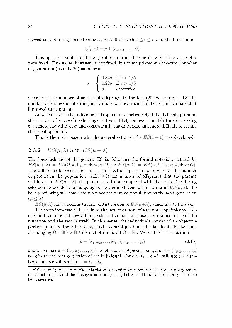
24 CHAPTER 2. EVOLUTIONARY ALGORITHMSviewed as, obtaining normal values si ∼ N(0, σ) with 1 ≤ i ≤ l, and the fun tion isψ(p, r) = p+ (s1, s2, . . . , sl)This operator would not be very dierent from the one in (2.9) if the value of σwere xed. This value, however, is not xed, but it is updated every ertain numberof generation (usually 20) as followsσ =

0.82σ if e < 1/51.22σ if e > 1/5σ otherwisewhere e is the number of su essful osprings in the last (20) generations. By thenumber of su essful ospring individuals we mean the number of individuals thatimproved their parent.As we an see, if the individual is trapped in a parti ularly di ult lo al optimum,the number of su essful osprings will very likely be less than 1/5 thus de reasingeven more the value of σ and onsequently making more and more di ult to es apethis lo al optimum.This is the main reason why the generalization of the ES(1 + 1) was developed.2.3.2 ES(µ, λ) and ES(µ+ λ)The basi s heme of the generi ES is, following the formal notation, dened by

ES(µ + λ) = EA(Ω, k,Πk, τ ; Ψ,Φ, σ;O) or ES(µ, λ) = EA(Ω, k,Πk, τ ; Ψ,Φ, σ;O).The dieren e between them is in the sele tion operator, µ represents the numberof parents in the population, while λ is the number of osprings that the parentswill have. In ES(µ+ λ), the parents are to be ompared with their ospring duringsele tion to de ide what is going to be the next generation, while in ES(µ, λ), thebest µ ospring will ompletely repla e the parents population as the next generation(µ ≤ λ).ES(µ, λ) an be seen as the non-elitist version of ES(µ+λ), whi h has full elitism5.The most important idea behind the new operators of the more sophisti ated ESsis to add a number of new values to the individuals, and use those values to dire t themutation and the sear h itself. In this sense, the individuals onsist of an obje tiveportion (namely, the values of xi) and a ontrol portion. This is ee tively the sameas hanging Ω = Rl1 × Rl2 instead of the usual Ω = Rl. We will use the notation

p = (x1, x2, . . . , xl1 ; c1, c2, . . . , cl2) (2.10)and we will use ~x = (x1, x2, . . . , xl1) to refer to the obje tive part, and ~c = (c1c2, . . . , cl2)to refer to the ontrol portion of the individual. For larity, we will still use the num-ber l, but we will set it to l = l1 + l2.5We mean by full elitism the behavior of a sele tion operator in whi h the only way for anindividual to be part of the next generation is by being better (in tness) and repla ing one of thelast generation.

2.3. EVOLUTIONARY STRATEGIES 25Observe that we an dene the fun tion τ(p) = ~x, as the ontrol values are notpart of the optimization pro ess.In these methods a deterministi ruleas the 1/5-rule, is no longer used. In-stead, we let the ontrol parameters to self-adapt, and add those parameters for ea hobje tive value.The ontrol parameters are also subje t to mutation and re ombination, whi h willallow evolution to sele t the best values of the parameters by itself. It is expe ted thatthose individuals with good ontrol values will end up having a good tness value,and in the long run, will give birth to better individuals.2.3.3 More operatorsThe obvious introdu tion of rossover operators surges from the availability of manyindividuals in the population. In ESs there are two types of rossover: sexual andpanmiti . In the sexual rossover, the ospring is generated by exa tly two parents,and in the panmiti rossover, we sele t one individual to play the role of one parent,and for every obje tive and ontrol value we hoose another random (with repla e-ment) parent. In the formal notation, the sexual rossover has values ri = 2, while inthe panmiti version, ri = l + 1.The panmiti version of the rossover operators reates more diversity in thepopulation, but slows down onvergen e. It is normally used in very di ult problems.Dis rete rossover The rst rossover operator used in ESs was the dis rete rossover. It onsists of inter hanging values from the parents to reate the ospring.This is very similar to the uniform rossover of the GAs. The formal fun tion is asfollowsφ(p, p′, r) = (q1, q2, . . . , ql) (2.11)where qi =

pi if si = 1p′i if si = 0where si ∈ 0, 1 is an uniform random number for 1 ≤ i ≤ l. The panmiti versionof this operator an be dened as

φ(p′, p1, p2, . . . pl, r) = (q1, q2, . . . , ql)where qi =

p′i if si = 1pi,i if si = 0

(2.12)This rossover is the easiest to ompute from all, but it is also the one withthe worst diversity. Observe that no new value is generated as we only generate anew individual with values already in the population. For this reason, even moresophisti ated operators were reated.

26 CHAPTER 2. EVOLUTIONARY ALGORITHMSIntermediate rossover The next used rossover operator is alled intermediate rossover, and was proposed, as its name implies, to make an ospring at the averageof two parents. The formal fun tion of this operator requires no random numbers(ex ept for the sele ted parents), and isφ(p, p′, r) = (

p1 + p′12

,p2 + p′2

2, . . . ,

pl + p′l2

) (2.13)and its panmiti version isφ(p′, p1, p2, . . . pl, r) = (

p′1 + p1,1

2,p′2 + p2,2

2, . . . ,

p′l + pl,l

2) (2.14)Observe that this rossover does reate new values for the individual. By alwaysaveraging two parents (in its sexual form), it tends to make the population onvergeeasily. By generalizing this idea of the average, new operators were proposed.Generalized intermediate rossover There also exists a generalized version ofthe intermediate rossover, to allow a weighted average of the two parents. Thisis known as the generalized intermediate rossover. The formal version requires anuniform random number η ∈ [0, 1], and the fun tion is

φ(p, p′, r) = (ηp1 + (1 − η)p′1, ηp2 + (1 − η)p′2, . . . , ηpl + (1 − η)p′l) (2.15)and the panmiti version isφ(p′, p1, p2, . . . , pl, r) = (ηp′1 +(1−η)p1,1, ηp

′2+(1−η)p2,2, . . . , ηp

′l +(1−η)pl,l) (2.16)Observe that this rossover has the possibility of generating new individuals alongthe line segment joining the two parents (in the sexual version). This notion an beeven more general, as we are still onning the sear h for osprings to a relativelysmall spa e.Generalized rossover The last rossover to dis uss here is alled generalized rossover, and reates osprings on the hyper- uboid with orners on the parents.That is, instead of using the same value as the weighted average of the parents, arandom value ηi ∈ [0, 1] is reated for ea h value 1 ≤ i ≤ k, and the weighted averageis reated for ea h value. The formal fun tion is

φ(p, p′, r) = (η1p1 + (1 − η1)p′1, η2p2 + (1 − η2)p

′2, . . . , ηlpl + (1 − ηl)p

′l) (2.17)and its panmiti version is

φ(p′, p1, p2, . . . , pl, r) = (η1p′1 + (1 − η1)p1,1, η2p

′2 + (1 − η2)p2,2, . . . , ηlp

′l + (1 − ηl)pl,l)(2.18)An important remark is that, unlike the GA's rossover operators, these operators an be applied to either only the obje tive values (~x) or to the ontrol values (~c), thusin reasing the mat hing possibilities to reate a omplete rossover operator.In general, it is used the generalized intermediate, or the generalized rossover onthe obje tive values, and dis rete on the ontrol values, but other ombinations areequally possible.

2.3. EVOLUTIONARY STRATEGIES 27Control mutation The natural way to extend the individuals is to add a ontrolparameter for ea h obje tive parameter to optimize. In this sense, the mutation willbe ontrolled by these parameters. In this ase, l1 = l2, and Ω = Rl1 × Rl1+, and thus

p = (~x;~σ) = (x1, x2, . . . , xl1 ; σ1, σ2, . . . , σl1) (2.19)Observe the dieren e against (2.10), in whi h only one ontrol value was used.As stated before, the ontrol values are not to be hanged by a deterministi rule,but by another me hanism.The ontrol mutator fun tion an be dened with l1 + 1 standard normal valuest′, ti ∼ N(0, 1), and l1 normal values si ∼ N(0, σi exp(τ ′′t′+τ ′ti)), for every 1 ≤ i ≤ l1.The fun tion is then dened asψ(p, r) = (~x+(s1, s2, . . . , sl1); σ1 exp(τ ′′t′+τ ′t1), σ2 exp(τ ′′t′+τ ′t2), . . . , σl1 exp(τ ′′t′+τ ′tl1))(2.20)where τ ′ = 1

4 4√

k1

and τ ′′ 1√2k1

. These values are parameters to ompensate the highdimensionality of some problems, and are fun tionally equivalent to the learning fa torused in arti ial neural networks. These onstants are usually referred to as τ and τ ′instead of τ ′ and τ ′′, however, due to the existen e of the mapping τ in the denitionof the EA, we opted to avoid the ambiguity by using an extra prime in the onstants.Observe that the values of the σ's are updated before the obje tive values, andalso, observe that only one random value is generated to be multiplied by τ ′′, whilenew random numbers are generated for every value to be multiplied by τ ′.Correlated mutation Another type of mutation proposed by S hwefel was the orrelated mutation, whi h main obje tive was to perform mutations in dire tionsnot aligned with the oordinate axis. By performing a rotation in spa e, we allow themutations to align with more general sear h dire tions, and make the optimizationpro ess faster.S hwefel observed that, in general, the path of one individual and its ospringis roughly perpendi ular to the optimal step (i.e. the ve tor joining the presentindividual to the optimal one). By this reason, a better dire tion an be used toallow a faster onvergen e ratio. A natural way to do this was to use the orrelationmatrix of the su essful osprings to hoose a dire tion. It has been proved, however,that the same ee t an be a hieved by using a series of anoni al rotation angles.A orrelated mutation is a hieved by rotating a non- orrelated mutation by anangle θ over one hyper-plane. The total number of angles required to dene everypossible rotation in an l1-dimensional spa e is ( l12

)

= l1(l1 − 1)/2. We an, then,dene Ω = Rl1 × Rl1+ × (−π, π]l1(l1−1)/2, whi h sets the individuals as

p = (~x, ~σ, ~θ) = (x1, . . . , xl1 ; σ1, . . . , σl1 , θ1, . . . , θl1(l1−1)/2) (2.21)where ~c = (~σ, ~θ), and l2 = l1 + l1(l1 − 1)/2.

28 CHAPTER 2. EVOLUTIONARY ALGORITHMSThis mutation operator is very similar to the ontrol mutation, ex ept that theθ's are updated before the obje tive values. That is, getting l1(l1 − 1)/2 standardnormal values αi ∼ N(0, 1), and l1 more normal values γi ∼ N(0, C(σ, θ)), the formaloperator an be regarded as

ψ(p, r) = (~x+ (γ1, . . . , γl1); σ1 exp(τ ′′t′ + τ ′t1), . . . , σl1 exp(τ ′′t′ + τ ′tl1); θ) (2.22)where β ≈ 0.0873, θ = ~θ + β(α1, α2, . . . , αl1(l1−1)/2), and C(σ, θ) is the ovarian ematrix. And one way to obtain this ovarian e dire tions is given in the next algorithmCovarian e dire tionsfor( i = 1 to l1 )∆xi = σi exp(τ ′′t′ + τ ′ti)si;for( m = l1(l1 − 1)/2 to 1 )(i, j) =indexOf(m); //Get the indexes that θm affe ts.∆xi = ∆xi cos θm − ∆xj sin θm;∆xj = ∆xi sin θm + ∆xj cos θm;for( i = 1 to l1 )xi = xi + ∆xi;As we an see, the dire tions are given in inverse order. This is due to the anoni altransformation in Euler's rotations in a k1-dimensional spa e, as the rotations end uprepresenting the produ t of the rotation matri es with rotation angle θm.2.3.4 A simple evolutionary strategy for onstrained optimiza-tionIn this se tion we will give an example of a simple evolutionary strategy to solve onstrained optimization problems using rules to rank individuals.The ES used is a ES(70 + 130), with ontrol individuals as in Equation 2.10,using intermediate generalized rossoverEquation(2.15) on obje tive values anddis rete rossover Equation (2.11) on ontrol values. The mutation used is thestandard for ontrol individuals as in Equation (2.20).The binary omparison fun tion used to sort the individuals for sele tion is thetotal violation rule explained in Se tion 1.3.2.2.This ES is used for omparison with the Baldwinian algorithms explained in Chap-ter 4.

2.4. MEMETIC ALGORITHMS 292.4 Memeti AlgorithmsAnother type of evolutionary algorithms are known as memeti algorithms (MA).They an be thought of as hybrid algorithms as they in orporate a lo al sear h intheir sear h pro ess [7.2.4.1 Denition of a MemeThe on ept of a meme was rst introdu ed by Dawkins [6, where he proposes aso ial equivalent to the gene as a basi unit for inheritan e. A ording to Dawkins,ideas evolve in ulture mu h like organisms evolve in biologi al evolution. The basi unit of ultural transmission is then alled a meme.Examples of memes are spoken senten es, written senten es, live musi , re ordedmusi , theater, inema and many more. They are the means by whi h we express ourideas, while the ideas themselves an be regarded as the phenotype of the meme.2.4.1.1 Memes and Lamar kismDawkins suggested that memes evolve by Lamar kian me hanisms. However, it ispossible that memes are a type of Darwinian evolution [20. When a human brainre eives a meme, the meme slowly matures into an idea. Eventually the host person an de ide to ommuni ate his idea to another person.This pro ess seem to be less Lamar kian than originally thought, as the hangedmeme itself (genotype) is not transmitted, but the idea (phenotype) instead. If thememe were hanged by an individual, it is not tra table to re ognize the meme, butperhaps the similarities that the idea (phenotype) has with the original meme; also,if the meme itself hanged, instead of just its representation, it would mean that areverse engineering pro ess a tually o urred in the host brain. Besides, the new hostre eives the idea, but the meme that olonizes this new host is dierent from thea tual idea he re eived, as the idea was transformed by the previous person.This might point to an internal evolution where the re eived meme intera ts withmany other memes in the host brain giving birth to new memes with rossover andmutation. The transmitted memes are also sele ted from a pool of memes inside thehost brain. These me hanisms tend to point to a Darwinian model of memes.Memes, though, are generally regarded a Lamar kian, and the denition of amemeti algorithm states this learly. This dis ussion will be useful, nevertheless,in Chapter 3, when we will try to reate a new algorithm based on the idea of non-Lamar kian lo al sear hes.2.4.2 Denition of a memeti algorithmFrom the point of view of the study of adaptive systems, it is the idea of memes asagents that an transform an individual what is of major interest. We an onsiderthe addition of a learning phase to the evolutionary y le as a form of memegene

30 CHAPTER 2. EVOLUTIONARY ALGORITHMSintera tion. This intera tion an aid evolution onsidering the genes to be plasti andallowing them to be guided by the learning me hanism.The basi idea behind MAs is to have at least one lo al sear h mutation operatoramong its operators (an in the evolutionary algorithm). This lo al sear h operator isusually applied after the rossover and mutation operators have been applied.The result of the lo al sear h repla es (Lamar kian) the individual if the foundsolution is better than the initial one. In this sense, if we have a lo al sear h algorithma : Ω → Ω that takes initial points and returns the result of the lo al sear h, thememeti learning an be viewed as

ψmemetic(p, r) =

p if f τ(a(p)) > f τ(p)a(p) if f τ(a(p)) ≤ f τ(p)A more rigorous denition of a lo al sear h algorithm an be found in Se tion 1.2.In general, the only thing that makes a MA dierent from other EAs is the in lusionof this other algorithm. The lo al sear h is used to smooth the tness lands ape aswe are now sear hing with evolution not on the normal sear h spa e, but on the setof lo al optimum solutions.Within a memeti algorithm, we an onsider the lo al sear h stage to o ur asan improvement within the evolutionary y le, and we should onsider if whether the hanges made to the individual should be kept or whether the improvement is onlyto ae t the tness asso iated with it.This idea is pre isely the motivation of this thesis, and will be dedi ated a Chapteron its own. In short, the de ision of whether the hange is made to the individual(a Lamar kian behavior) or to the tness (a Darwinian behavior) is what makes thedieren e between the memeti algorithms and the Baldwinian algorithms.All this might make more sense if we think of meme evolution as a Darwinianme hanism instead of a Lamar kian one. Turney [20 gives reasons why memes arenot ne essarily Lamar kian, as well as reasons why memes ould be Baldwinian. Thisdis ussion might be relevant to de ide whether the name memeti algorithm is amisnomer or not, but is not of dire t interest to this thesis.2.5 Dierential EvolutionOne of the most re ent and famous evolutionary algorithms in the literature is thedierential evolution (DE). Created by Pri e and Storn [15, the DE is a little dierentfrom traditional evolutionary algorithms in the sense that it has only one operatorto perform all the sear hing pro ess. It is, in ontrast to geneti algorithms andevolutionary strategies, not based on re ombination and mutation to perform thesear h, but on a more mathemati al than biologi al operator that gives his name tothe algorithm.The basi idea behind DE is to take the dieren e of two randomly hosen ve torsin the population and make a weighted sum of this dieren e with another randomly

2.5. DIFFERENTIAL EVOLUTION 31 hosen ve tor and ompare it with the original one to pla e a new individual for thenext generation. If this new individual turns out to be better than the individual inthe urrent position, then the old individual is repla ed by the new one.Be ause no rossover is performed, DE is highly sus eptible to parallelization. Itis also fast and e ient for global optimization, and it also has a small number ofparameters, whi h have, in great measure, won for itself most of its fame.2.5.1 The DE_1 algorithmThe formal spe i ation of the dierential evolution an be regarded as DE_1(F ) =EA(Ω, k,Πk, τ ; Ψ,Φ, σ;O), where Ω = Rl, the fun tion τ is the identity, and Φ is alsothe identity (i.e. no rossover), thus O = Ψ, and the sele tion me hanism is as follows

σ(P,Q, r) = (b1, b2, . . . , bl)where bi = arg maxf τ(pi), f τ(qi)i.e. it ompares only the individuals at orresponding positions in the urrent popu-lation P and the newly generated one Q.The individuals are ve tors dened byp = (x1, x2, . . . , xl)The only mutation operator is, as des ribed above, what gives its name to thedierential evolution, and the lassi al one is dened next. Getting random integernumbers s1, s2, s3 ∈ 1, 2, . . . , k without repla ement from r, the dieren e operator an be dened as

ψ(p, r) = ps1+ F (ps2

− ps3) (2.23)Observe that the only thing that matters about the parameter p is its position inthe urrent population P , as it is not used to de ide the new ve tor generated by ψ.On e we have generated the population Pf from the population Pi, we an pro eedto sele tion, and then to the iterative step in the evolutionary algorithm.The parameter F ontrols the strength of the dieren e operator. It is usually lose to 1, but depend on the size k of the population. If the population size is small,a F = 1 should be used, if the population size is large, a F ≤ 0.9 should work ne.This is due to the spe ial behavior of the dieren e operator. Mathemati ally,if the population is near onvergen e, it is expe ted that the operator will reatesmall hanges6, on the other hand, if we take one good solution with a bad one forthe dieren e, the rough dire tion of the dieren e will be towards the optimum (or ompletely away from it if it has the opposite sign), this is why it manages to ndoptimal solution while sear hing.This method has the risk, however, of premature onvergen e, and as it does nothave a me hanism to avoid it, several runs might be ne essary to a hieve the a tualoptimum.6The dieren e among two ve tors will be small if the individuals are lose enough.

32 CHAPTER 2. EVOLUTIONARY ALGORITHMSThe sele tion pressure of this EA is also interesting to analyze. As one individualis only ompared to a newly generated one in the sele tion pro ess, it is fairly easythat the worst individual will survive. In fa t, when in the middle of the pro ess, theworst individual so far might very well survive for several generations if is has a bit oflu k. This might suggest that the sele tion pressure of the sele tion operator is weak.On the other hand, however, on e a luster of the population starts to onverge,the probability of having new individuals generated near that luster in reases veryqui kly, thus reating a y le in whi h more and more individuals are dragged tothis zone. In onsequen e, the sele tion pressure for individuals far from this lusterin reases almost exponentially.In on lusion, dierential evolution seems to have, impli itly, a self-adaptive se-le tion pressure, starting weak and maintaining so for several generations, and thenabruptly starting to grow to the point in whi h no new solutions out of the (sub)optimal luster are tolerated by the sele tion operator.2.5.2 The DE_2 algorithmThe se ond variation known as DE_2(λ, F ) is somehow based on parti le swarmoptimization as it uses the urrent best found solution to dire t the sear h. Formally,this dieren e operator an be regarded asψ(p, r) = ps1

+ λ(pb − ps1) + F (ps2

− ps3) (2.24)where pb = arg max

1≤i≤kf τ(pi)and the variable λ is a ontrol value used to ontrol the greediness towards the bestsolution so far. It should be small normally, unless the global optimum is relativelyeasy to nd.2.5.3 More operatorsAs is usually the ase with evolutionary algorithms, there is a number of other oper-ators used to improve the performan e of the DE algorithm.Here we will only dis uss the pseudo- rossover performed to in rease the diversityin the population. When this operator is working, it is used over one of the dieren eoperators explained in Equation (2.23) and in (2.24). This operator requires anothervariable, CR, representing the rossover rate. It is usually set to a high value (near

1), ex ept for easy optimization problems.Suppose the fun tion ψ′ is dened as either (2.23) or (2.24), and obtain two randomintegers d ∈ 1, 2, . . . , l and L su h that P (L ≥ v) = (CR)v−1, v > 0. The newmutation (pseudo- rossover) operator is dened asψ(p, r) = (v1, v2, . . . , vl)where vj =

ψ′(p, r)j if d ≡ d, d+ 1, . . . , d+ L− 1(mod l)pj otherwise

2.5. DIFFERENTIAL EVOLUTION 33where ψ′(p, r)j is the j-th value of the ve tor ψ′(p, r).

Figure 2.5: The s hemati view of the pseudo- rossover operator for dierential evo-lution. We an observe that the rossed ve tor has 3 values of the original ve tor,and 3 from the new one.The sket h of this operator an be observed in Figure 2.5. The individual depi tedthere has length l = 6, the values used for the pseudo- rossover are d = 5 and L = 3,and then the new individual shares three values with the original one, and three withthe new one, beginning at d and ir ling around in a modular fashion. This operatorresembles the two-point rossover of GAs.2.5.4 Dierential evolution for onstrained optimizationIn this se tion we will give an example of a simple evolutionary strategy to solve onstrained optimization problems using rules to rank individuals. As in Se tion2.3.4, we will adapt the DE_1 to solve a ben hmark of onstrained optimizationproblems.The DE pi ked uses the pseudo- rossover operator mentioned above, and it isthen stated as a DE_1(0.9, 0.9), with normal parameters. The binary omparisonfun tion used to a ept individuals in sele tion is the total violation rule explained inSe tion 1.3.2.2.This DE is used for omparison with the Baldwinian algorithms in Chapter 4.

34 CHAPTER 2. EVOLUTIONARY ALGORITHMS

Chapter 3The Baldwin Ee tMany resear her have drawn analogies between learning and evolution as two intel-ligent pro esses, one taking pla e during the lifetime of an organism, and the othertaking pla e over the evolutionary history of life on Earth. We tend to regard theevolutionary pro ess as adaptive and intelligent in the sense that individuals are(sub)optimal solutions to the problem of staying alive. In this sense, there is an opti-mization pro ess undergoing evolution. The question remains, though, as if learning an have an impa t at all in the evolutionary me hanisms in nature, and if so, towhat extent.Sin e the moment in 1987 that Hinton and Nowlan [10 published their lassi pa-per, a large number of resear her have worked in experiments on erning the BaldwinEe t in evolutionary omputation[14, 2. Many of them have also observed the syn-ergi ee t that learning1 an have in the evolutionary me hanisms when there is anevolving population of individuals. This synergy is what is usually alled the BaldwinEe t. In general, there seems to exist a misunderstanding of the real aspe ts behindthis ee t, and, apparently, the resear hers have left aside another equally importantaspe t of it.At a rst approa h, we an think of the whole Baldwin Ee t as a two-sided oin.In one fa e, one has the observed behavior that lifetime learning an, under ertain ir umstan es, a elerate the evolutionary pro ess in a population. In the other one,we must take into a ount that it is ostly for an individual to learn.In this line, there is indeed a synergy ee t that an o ur during evolution withindividuals that are able to learn, but there is also a ost asso iated with that learningability. The Baldwin Ee t is on erned with both aspe ts.This hapter is mainly on erned with the understanding of the Baldwin Ee t asa biologi al me hanism that may or may not be present in nature, but that an be ofuse for the evolutionary omputation ommunity as a new sear h strategy. It is alsothe aim to demystify the relation between Lamar kism and Baldwinism in a system,and the possible uses that both may have in optimization problems.1A tually, phenotypi plasti ity, but we will talk about it later in this hapter.35

36 CHAPTER 3. THE BALDWIN EFFECT3.1 Basi Con eptsIn order to fully understand the Baldwin Ee t, a number of on epts must be de-veloped in advan e. The Baldwin Ee t is a misnomer be ause it was dis overedindependently by Baldwin, Morgan and Osborn (1896), and also be ause it is not asingle ee t, but rather a luster of ee ts or observations.It is relatively well know the dieren e between the genotype and the phenotype.The genotype stands for the internal heritable material of an individual, it odes thenal utter aspe ts of the individual in a persistent and un hangeable2 way. It is typ-i ally represented by the organism's DNA. It obtains its name from the genes, whi hare onsidered the atoms of inheritan e. On the other hand, the phenotype is thephysi al realization of an organism's genotype. It refers to every represented aspe tthat was impli it in the geneti ode, and was developed as part of the individual.It in ludes from the body omposition to the behavioral traits, and the abilities toadapt any of these based on an inherited hara teristi . They an be viewed as theobservable aspe ts of the organism's genotype. It obtains its name from the Greekword phainein, whi h means to show.The key term in the Baldwin Ee t is known as phenotypi plasti ity, whi h an beregarded as the ability of an organism to adapt to its environment due to the featuresof the phenotype. There are many examples of phenotypi plasti ity in nature, mostof whi h have a dire t relation with the organism's body in its environment; forinstan e the ability of the skin to tan when exposed to the Sun, or to form alluswhen onstantly abraded, or many onditioned behaviors a quired by asso iation3.Another on ept is the notion of lifetime learning, whi h is the set of learning thathappens during the lifetime of an individual. It is only on erned with the learningmade by a single individual and not with the ma ros opi population level of learningin whi h the evolution may fall into. The impa t of lifetime learning on evolution isonly one example of the Baldwin Ee t; in its most general sense, it deals with theimpa t of phenotypi plasti ity as a whole, on the evolution of a spe ies.In ontrast to the phenotypi plasti ity, we all phenotypi rigidity the inabilityof an individual to adapt to a new problem. This inability, ontrary to what theintuition di tates us, may be an advantage over more plasti individuals. We willexplore this in more detail.3.1.1 Benets of phenotypi rigidityPhenotypi rigidity an be advantageous to an organism in many situations. A hard- oded behavior is potentially less hazardous to an individual than a plasti one. Forexample, learning requires experimentation, and in the ase of a potentially fatal2Not quite un hangeable sin e the individual an mutate, but in general terms it is not sus eptibleto hanges.3Like the famous Ivan Pavlov's experiments on onditioned response on dogs.

3.1. BASIC CONCEPTS 37behaviors4, instin t will ertainly have an advantage over learning, be ause an indi-vidual will be born with a natural avoidan e behavior instead of with trial-and-errorlearning ability. Another example ould be the time required to form a allus whi h ould be used in some other a tivities if the organism were born with a thi k skin5.In general, an individual with an instin tive behavior, will require mu h less energyand will save time. The behaviors are ready for him to use at birth-time. In on-trast, plasti ity oers the possibility to adapt, but the ost of developing the requiredbehavior, has potentially fatal onsequen es.3.1.2 Benets of phenotypi plasti ityIn ontrast, phenotypi plasti ity enables an organism to explore new possibilities ofpotentially better behaviors. This may be a great advantage in hanging environmentsor in environments that abruptly hanged and are to remain so. The spe ializationis an observed hara teristi of phenotypi rigidity, but an lead to a disaster whentaken to the limit6. If the rigidity will not allow an individual to adapt to an already hanged environment, then, learly the plasti ity will bestow the individual that hasit with an evolutionary advantage over those who does not have it.In general terms, the phenotypi plasti ity smooths the tness lands ape enablingthe organism to explore neighboring areas of the phenotype spa e, and thus allowingthe individual to have an ee tive tness of a lo al maximum in this spa e. If a ertain ontinuity in the mapping from genotype to phenotype is assumed, a (potentially)worst genotype would have a better tness through plasti ity than a better genotype.Behaviors tend to be more plasti than physi al stru tures. The pro ess of learninga behavior represents appropriate hanges in the nervous system, and it is in generaltrue that the nervous system of an organism is more exible than many other physi alstru tures.3.1.3 Lamar kism and Baldwin Ee tThe Lamar kian hypothesis states that the traits a quired during an organism lifetime an be transmitted via inheritan e to the organism's osprings. This hypothesis isgenerally interpreted as referring to a quired physi al traits7, but something learnedduring lifetime an also be onsidered an a quired trait.To put it in simple terms, Lamar k says that the son of an athlete is more likelyto be a good athlete, and the son of a s ientist tends to be more intelligent. Thus, aLamar kian view would hold that learned knowledge an (and will) guide evolution bydire tly passing the knowledge to the next generation. However, due to overwhelmingeviden e against it, the Lamar kian hypothesis has been reje ted by virtually all4Like learning not to eat a poisonous fruit.5For example the elephant.6As is the ase with the Koala, whose diet is onned to a single dish: the eu alyptus' leaves7Su h as physi al defe ts due to environmental toxins

38 CHAPTER 3. THE BALDWIN EFFECTbiologists. Lamar kism requires an inverse mapping from phenotype and environmentto genotype, and this mapping is biologi ally implausible [14, 20.It would seem that the reje tion of the Lamar kian hypothesis leaves out thequestion of if learning has any impa t on evolution, but the answer seems to be thatlearning an indeed have a signi ant ee t, though in a less dire t way than Lamar ksuggested. The Baldwin Ee t is purely Darwinian (in ontrast to Lamar kism) andit does not involve any reverse mapping.Suppose the typi al example of Lamar kism, with a short-ne ked animal thatlearns to stret h its ne k to rea h leaves on a tall tree. Lamar k believed that theanimal's osprings would inherit slightly longer ne ks than they would otherwise havehad. It requires a me hanism for modifying the parent's genes based on the habit ofstret hing its ne k.The Baldwin Ee t has observable onsequen es that are similar to Lamar kianevolution. Baldwin would have pointed that if stret hing their ne ks helps towardstheir survival, then the organisms that are more able to learn to stret h their ne kswill have the most ospring, thus ee tively in reasing the frequen y of the genesresponsible for learning. In this sense, if the environment remains relatively xed,so that the best thing to learn remain onstant, this an lead, via sele tion, to apopulation of animals very good at stret hing their ne ks.There an be advantages, however, in being born with a longer ne k. And it isbelieved that if given enough time, the evolution pro ess will be able to evolve longerne ks in the population, whi h will lead in its turn, to a geneti al en oding of longerne ks.One may view this pro ess as if the Baldwin Ee t were Lamar kian in its results,but not Lamar kian in its me hanism. Given a desirable trait, the Baldwin Ee tonly provides the required time (via a quiring the trait due to phenotypi plasti ity)for the trait to appear in the population's genes (via the evolutionary pro ess).3.1.4 The Darwinian me hanismThe evolutionary biologist G. G. Simpson, studied the onje tures made by Baldwin[19 and pointed out that it is not lear how the ne essary orrelation between phe-notypi plasti ity and geneti variation an take pla e. We mean by orrelation therequirement that geneti variations happen to o ur and produ e the same adapta-tion that was previously learned. This kind of orrelation would be easy understoodif geneti variations were dire ted towards some parti ular out ome rather than atrandom. But randomness is entral in modern evolution theory, espe ially on erninggeneti variation, and a spe i orrelation would mean a Lamar kian me hanism forevolution.It seems that Baldwin was assuming that, given the laws of probability, orrelationbetween phenotypi adaptations and random geneti variation will happen, espe iallyif the phenotypi adaptations keep the lineage alive long enough for these variationto o ur. It does not point, however, to a spe i orrelation among them. Simpson

3.2. BALDWIN EFFECT AND COMPUTER SCIENCE 39agreed that this was possible in prin iple, but remains unknown if it is an importantfor e in evolution.While it appears that we are at a dead end, it may not be the ase, as the answerto that question may be found in the work of Waddington [22, who proposed a me h-anism alled geneti assimilation. This me hanism is on erned with the inheritan eof a quired traits, but tries to explain the underlying pro ess from a slightly dier-ent point of view. It states that some sudden and potentially deadly hanges in anenvironment would require phenotypi adaptation that are not ne essary in normalenvironments. If organisms are subje t to su h hanges, they an sometimes adaptduring its lifetime be ause of their inherent plasti ity, thereby a quiring new physi alor behavioral traits. If the genes of these traits are already in the population, butare dormant8, they an fairly qui kly be expressed in the hanged environments, andas in the Baldwin Ee t ase, espe ially if the a quired traits prevent the individualsfrom dying.Waddington even demonstrated that it has happened in several experiments onfruit ies. It suers, however, of the same skepti al point of view oered by Simpson:there is no nal proof that this ee t is indeed an important for e in evolution.However, although the geneti assimilation is better known in the evolutionary biology ommunity than the Baldwin Ee t is, the later has been re ently pi ked up byevolutionary omputing resear hers mainly be ause of the experiment made by Hintonand Nowlan, and be ause it has proven useful in several resear h areas.3.2 Baldwin Ee t and Computer S ien eThere is a ommon feeling to think that learning is always good, at least that iswhat our nature tends to tell us. As we have observed before, this may not alwaysbe the ase, and this might be parti ularly true when onfronted to the world of omputers, when CPU time and memory requirements are ru ial in the analysis ofa new algorithm. Evolution is onstantly sele ting the best balan e between learningand instin t, and this balan e is usually not xed during all the optimization pro ess.It varies dramati ally when spe ies are onfronted with an abrupt hange in theirenvironment and also when the environment has a hieved an epistati state9.There is a number of interesting experiments applying the Baldwin Ee t to evo-lutionary omputing on various settings, mainly dedi ated to observe the intera tionsbetween learning and instin t. Peter Turney [20 presented a list of observations,based on the fundamental insight that there are trade-os between learning and in-stin t10, and are reprodu ed in Table 3.1.8Here we say that a gene is dormant if it is not usually expressed in the population's phenotype,in ontrast to expressed if the trait it odes a tually appears in the population.9Roughly speaking, an state in whi h there are no more sudden hanges.10We have been using learning as a form of phenotypi plasti ity and instin t as phenotypi rigidity,the generalization to other kinds of phenotypi behaviors is fairly straightforward and is left to thereader.

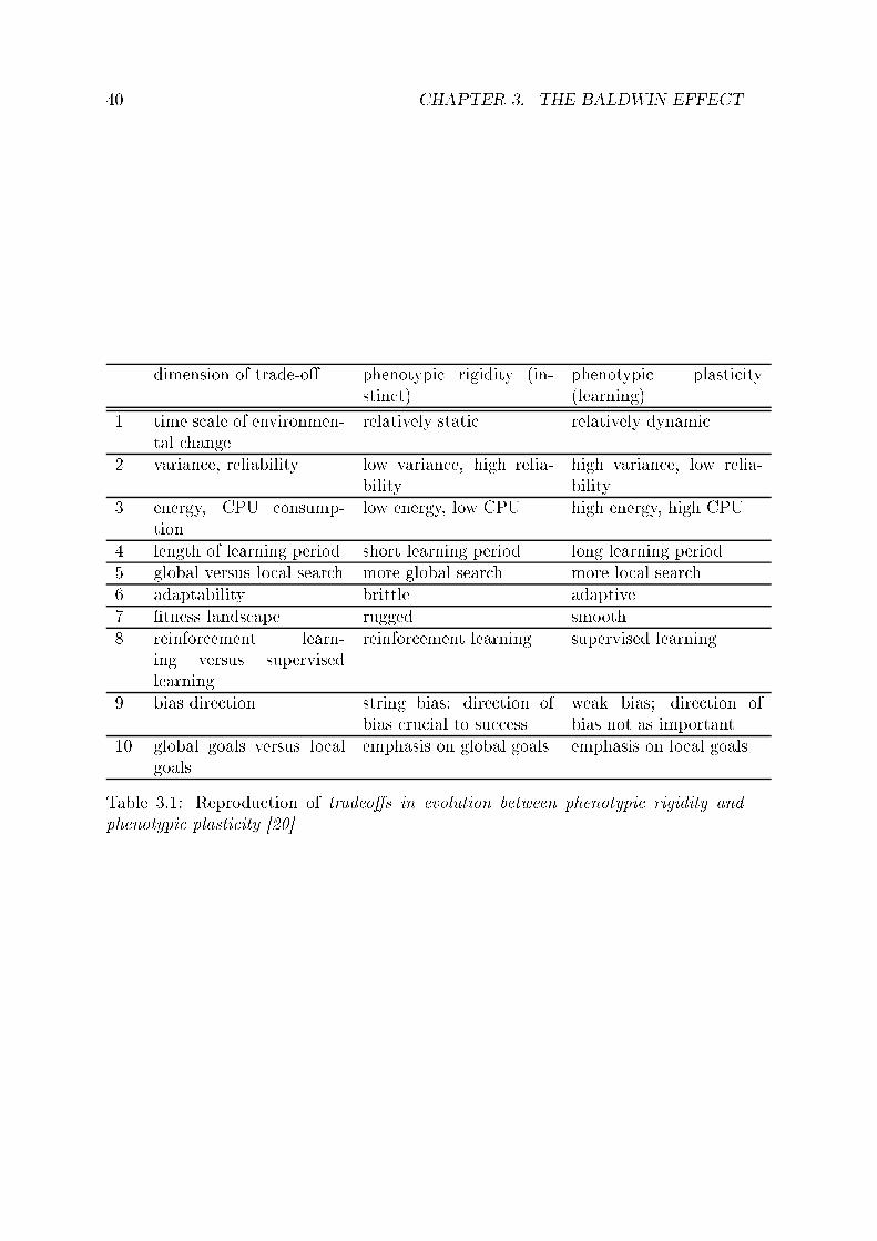
40 CHAPTER 3. THE BALDWIN EFFECT

dimension of trade-o phenotypi rigidity (in-stin t) phenotypi plasti ity(learning)1 time s ale of environmen-tal hange relatively stati relatively dynami 2 varian e, reliability low varian e, high relia-bility high varian e, low relia-bility3 energy, CPU onsump-tion low energy, low CPU high energy, high CPU4 length of learning period short learning period long learning period5 global versus lo al sear h more global sear h more lo al sear h6 adaptability brittle adaptive7 tness lands ape rugged smooth8 reinfor ement learn-ing versus supervisedlearning reinfor ement learning supervised learning9 bias dire tion string bias; dire tion ofbias ru ial to su ess weak bias; dire tion ofbias not as important10 global goals versus lo algoals emphasis on global goals emphasis on lo al goalsTable 3.1: Reprodu tion of tradeos in evolution between phenotypi rigidity andphenotypi plasti ity [20

3.2. BALDWIN EFFECT AND COMPUTER SCIENCE 41A ording to Turney [20, the ourse of the balan e is not the main on ern ofthe Baldwin Ee t, but the fa t that there are trade-os. In this sense, we try toexamine the trade-os oered by Turney in order to larify the possible appli ationsof the Baldwin Ee t.Time s ale of environmental hange. Evolution and learning operate at dierent times ales. In a dynami environment, evolution annot adapt fast enough,so learning is better. In a stati environment, evolution an adapt, solearning is a waste of time.Varian e and reliability. Learning is heavily based on experien e and requires that theright kind of experien e is present in order to a quire the desired learnedbehavior. This makes learning more sto hasti than instin t. Learning in- rements the variation in the population (dierent stimuli lead to dierentbehaviors) whi h an aid evolution.Energy and CPU onsumption. Any individual must expend energy in order to learn.The lo al sear h asso iated with learning onsumes evaluation of the t-ness fun tion (CPU time), and less resour es are left for evolution.Length of learning period On e an individual is born, it must dedi ate some timeto learn a trait, if it is instin tive, it is available at birth-time. Shorterlearning times are usually preferred by evolution.Global versus lo al sear h. Evolution performs a global sear h, while individuals per-form a lo al sear h (in phenotypi spa e). This trade-o varies greatlydepending on the stage of the evolution and the urrent population.Adaptability. Learning is more able to adapt to a variation in the environment whileinstin t tends to be brittle.Fitness lands ape. Learning, as dis ussed before, smooths the tness lands ape ef-fe tively removing rugged areas in the phenotypi sear h spa e. It is onlyadvantageous if the lands ape was not already smooth in whi h ase it isless useful.Reinfor ement versus supervised learning. An evolutionary algorithm is a type of re-infor ement learning for high tness areas of the sear h spa e. In termsof feedba k from the environment, it is situated somewhere between un-supervised and supervised learning. Supervised learning obtains morefeedba k from the environment and is more alike to the lo al sear h per-formed by learning as phenotypi plasti ity.Bias dire tion. The bias is a term widely used in ma hine learning, but has re entlyattra ted the attention of the onstrained optimization ommunity. Thebias dire tion has two omponents, the dire tion and the strength. If the

42 CHAPTER 3. THE BALDWIN EFFECTdire tion is wrong to a ertain problem, the strength will either allow orrestri t the exploration pro ess of the algorithm, and learning is bettersuited. If the dire tion is orre t, an strong bias (instin t) will be bettersuited for the problem.Global versus lo al goals. Evolution and learning have dierent goals. Evolutionseeks to maximize tness while individuals have more immediate goals.Learning is used by individuals to help them a hieve their immediate goalsin a better way. It is usually said in Game Theory that every individualmust pursue its own (simple) goals for the global (more omplex) goals tobe fullled, and in this sense, yet again we get a synergy from learning toevolution.As explained before, the trade-os shown here are not exhaustive and, as Turneyhimself says, there may be some overlap in the terms. The list will tend to grow asnew aspe ts of the Baldwin Ee t are known, and new appli ations are found for it.3.2.1 Hinton and Nowlan's experimentSome re ent work in Geneti Algorithms has been dire ted towards the analysis ofthe benets of phenotypi plasti ity, phenotypi rigidity and the plasti ity of learning.Perhaps the rst attempt made in this dire tion was performed by Hinton and Nowlan[10 as stated at the beginning of this hapter.Their observations seem to imply that learning an fa ilitate evolution but theselearned behaviors will eventually be repla ed by instin tive behaviors if the environ-ment remains onstant during a relatively long time. An extremely simple neural-network11 learning algorithm was reated to model learning in a population. Everyindividual in the population odies a andidate for solution to the neural network,thus a geneti algorithm played the role of evolution on the population of evolvingindividuals with learning apabilities.In this simplied model, every individual onsists of 20 potential onne tionsamong neurons. A onne tion an have one of three values: present, absent, andlearnable; whi h are oded as 1, 0 and ? respe tively, where ea h question mark an be set during learning to either 0 or 1. Then, the representation is a stringof 20 values, so an individual is represented by a1a2 . . . a20 where ai ∈ 0, 1, ? forea h i ∈ 1, 2, . . . , 20. There is only one orre t setting of the neural network's onne tions (whi h, by simpli ity is all present12), and no other setting onfers anytness to the individual. We will say that a onne tion is xed if it is either 0 or 1,and that it is not xed if it has a question mark.The problem to be solved is to nd this single orre t set of onne tions. Is willnot be possible for those networks that have in orre t xed onne tions to nd the11Whi h is a tually transparent to the pro ess, so no prior knowledge about arti ial neuralnetworks is required to understand it.12This means all the onne tions present, or, as an individual, a hromosome onsisting of 20 ones.

3.2. BALDWIN EFFECT AND COMPUTER SCIENCE 43solution, but those networks that have orre t values in all xed pla es, have theopportunity to learn the orre t setting. In this experiment, the simplest learningmethod was used: random guessing. On ea h trial, an individual guesses 0 or 1 atrandom (uniform) on ea h question mark it possesses.This problem is, by design, a needle in a haysta k sear h problem, sin e there isonly one orre t setting out of the 220 possibilities. The tness lands ape for thisproblem is s hemati ally represented in Figure 3.1the single spike represents thesingle orre t onne tion setting. Introdu ing the ability to learn, as expe ted by the

Figure 3.1: S hemati view of the tness lands ape for Hinton and Nowlan's sear hproblem. All genotypes have tness 0 ex ept for the orre t one with tness 1.Baldwin Ee t, the lands ape it smoother, and now we observe in Figure 3.2 a zoneof in reased tness, meaning that there are individuals that an learn the orre tsetting and have a reward of tness (inversely proportional to the number of trials).This zone in ludes individuals with only orre t xed positions and question marks.On e the individual is inside this zone, evolution makes it possible to limb to thepeak.The initial population onsisted of 1000 individuals, ea h onsisting of 20 genes,generated at random, with ea h gene having probability 0.25 of being 0, probability0.25 of being 1, and probability 0.5 of question mark. At ea h generation, ea hindividual was given 1000 learning trials. On ea h learning trial, the individual trieda random ombination of settings for the question marks.The tness was al ulated by the following formula,

Fitness = 1 +19(1000− i)

1000(3.1)where i stands for the number of trial in whi h the individual guessed the orre tsetting of onne tions. The tness is an inverse fun tion of the number of trials needed

44 CHAPTER 3. THE BALDWIN EFFECT

Figure 3.2: S hemati tness lands ape after learning.The sear h problem is smoother with a zone of in reased tness ontaining individualable to learn the orre t onne tion settings.by an individual to nd the orre t solution. With this fun tion, an individual withall its positions xed and equal to 1, would get the maximum tness value of 20, whilean individual that was never able to orre tly guess the solution or that has at leastone wrong xed position would get the minimum tness value of 1.In this experiment we an observe the trade-o of the Baldwin Ee t as manyquestion marks mean that, on average, many guesses are needed to arrive to thesolution, but the more xed positions, the more likely it is that at least one value iswrong thus ee tively killing the individual. This trade-o depi ts the one existingbetween e ien y and plasti ity in a very straightforward way.In expe tation, an individual has half of its positions xed in the initial population.The expe ted number of individuals in the initial population that have no wrong xedposition is about one (the 210 possible values for half xed positions are about 1000).In the ending, it is expe ted that at least one individual will be able to learn the orre t settings, but this is no surprise be ause 1000 ∗ 1000 = 106 ∼ 220, so thisexperiment ould be onsidered invalid be ause of this analysis, however, it is anexample of a simple experiment and the ability of the Baldwin Ee t to smooth thetness lands ape, as it was stated by Mit hell [14 that the mean tness was notobserved to improve over generations in the ase of pure evolution.Hinton and Nowlan's geneti algorithm used to solve this problem was very similarto the simple geneti algorithm dis ussed in Se tion 2.2. The sele tion me hanismwas by roulette wheel, with repla ement. They used one-point rossover and simplemutation; also, the hromosome of the individual was obviously not ae ted by learn-ing that took pla e during its lifetime. Originally, they let the algorithm run for 50generations. They observed that 0 genes were rapidly eliminated from the population

3.2. BALDWIN EFFECT AND COMPUTER SCIENCE 45

Figure 3.3: Relative frequen ies of 1's (dotted), 0's (dashed) and unde ided (solid)alleles in the population plotted over 50 generations.

46 CHAPTER 3. THE BALDWIN EFFECTand that the frequen y of 1's in reased a ordingly. In Figure 3.3 we show the relativefrequen ies of orre t (ones), in orre t (zeros) and unde ided (question marks) allelesin the population plotted over 50 generations.3.2.1.1 Harvey's experimentThe main on ern resulting from the plot is why did the frequen y of unde ided allelesstays so high. With the frequen y of question marks stable at 45%, and the frequen yof 1's stable at 55%, an average individual with 20 genes would have eleven 1's andnine ?'s. A more detailed study of this experiment was performed by Harvey [9,and Belew [3, and a ording to them, the expe ted tness of su h an individual isroughly 11.6. Also, they performed an statisti al analysis of the expe ted tness ofthe algorithm if only evolution was allowed to sear h (i.e. not learning), and resultedat 1.009.This points learly to the rst aspe t of the Baldwin Ee t, in whi h learning aidedevolution to improve the expe ted tness from 1.009 to 11.6, but this experiment, as itwas made, did not say mu h about the evolution's preferen e of instin t over learningon the long term. To answer this question, Harvey [9 reprodu ed and augmented theoriginal experiment in order to address the so- alled Puzzle of the persistent questionmarks. In his work, he ran the model for 500 generations, and he observed that thefrequen y of question marks indeed de reased in time towards 0%. However, it didnot matter how many generation he ran the model, that per entage never rea hedzero.The reason seems to be the geneti drift, due to random mutation in the pop-ulation. Mutation exerts a onstant pressure that maintains a ertain frequen y ofunde ided alleles in the population, and eventually, the population will a hieve anequilibrium state where the pressure of geneti drift balan es with the sele tion pres-sure that favors instin t.3.2.2 Turney's experimentsWe will analyze now a model that is a bit loser to a more omplete Baldwinians enario. In his paper, Turney [21 used the Baldwin Ee t as a method to shiftthe bias in a ma hine learning problem. His experiment is also simple as he arguesthat a more omplex experiment would only obs ure the role of Baldwinism in theoptimization pro ess. His work is of interest to us sin e he introdu es a new type of oding for learning in the genotype. In order to understand his work, we will have todevelop a few on epts.3.2.2.1 Denition and types of biasEx luding the input data, every fa tor that inuen es the sele tion of one parti ular on ept (in ma hine learning) onstitute the bias of a learning algorithm. Bias in- ludes su h fa tors as the language in whi h the learner expresses its on epts, the

3.2. BALDWIN EFFECT AND COMPUTER SCIENCE 47algorithm used to sear h the spa e, and the riterion for de iding whether a on eptis ompatible with the training data.As we saw at the beginning of Se tion 3.2, the bias onsists of two fa tors: dire tionand strength. A orre t bias is one that allows the on ept learner to sele t the target on ept. The orre tness of the dire tion is thus measured by the performan e of thelearned on ept on a test data. A strong bias is one that fo uses the on ept learneron a relatively small number of on epts.3.2.2.2 Shift of biasA growing body of resear h in ma hine learning is on erned with algorithms thatshift bias as they a quire more experien e. Shift of bias performs two levels of sear h,one through on ept spa e and one through bias spa e.We have seen that a strong bias is somewhat analogous to an instin tive behavior,while a weak bias is to a learned behavior. The ost of having a strong bias is thatthe bias an be in orre t, and the disadvantage of having a weak bias is a poorperforman e or e ien y on the long term. Unless we have high onden e that thebias is orre t, it is in general risky to have a strong bias. All of this is in a ordan eto the Baldwin Ee t, so it seems reasonable to in orporate it as a bias shifter.3.2.2.3 The Baldwinian modelTurney generalized the experiment of Hinton and Nowlan and adapted it to thema hine learning problem as a shift of bias problem. It may not be lear that a shiftof bias was used in Hinton and Nowlan's experiment, but we might see the amountof question marks as the strength of the bias. Having many unde ided alleles wouldresult in a weak bias, while having just a few would result in a stronger bias. The plotof question marks' frequen ies in the population an be regarded as the population'straje tory of sear h in bias spa e. For this new experiment, this distin tion is madeexpli itly, and might be laried better with the experiment itself.Let us onsider the example of on ept learning. Suppose the examples to lassifyare all ve-dimensional Boolean ve tors ~x ∈ 0, 15, and that they may belong to oneof two lasses 0, 1. By simpli ity, let us all this spa e T = 0, 15. In this sense, thesear h spa e of on epts is the spa e of fun tions F = f |f : T → 0, 1, mappingve tors to lasses. To simplify the notation, we see that it is possible to identify ea h on ept (i.e. ea h fun tion in F ) with its truth table. The truth table lists all of the25 = 32 possible ve tors in lexi ographi al order, and the value of the fun tion forea h ve tor. As the ve tors are in lexi ographi al order13, we an impli itly assumethe ve tors in the truth table, and ompa tly write the asso iations of the fun tionas a 32-bit string, with the i-th position in the string orresponding to the lass ofthe i-th 5 -bit ve tor.13A tually, any order may work.

48 CHAPTER 3. THE BALDWIN EFFECTFor example, the fun tion that maps every ve tor ~x ∈ T to 1, would be odedas the bit string onsisting of 32 ones, and onversely; the binary string given by11101111111101111111110111111111 represents the fun tion that maps the ve tors00011, 01100 and 10110 14 to the lass 0, and the rest to the lass 1. In this way, wehave a total of 232 = 4294967296 possible fun tions, and thus, the amount of possiblesolutions to the lassier problem are also 232.Suppose that one parti ular target on ept is what we want to nd, as was the asewith Hinton and Nowlan's neural network. To fa ilitate omparison with Harvey [9,we will suppose that the target fun tion is the fun tion that lassies every ve tor tothe lass 1 (i.e., f(~x) = 1 for ea h ~x ∈ T ). We assume, also, the standard supervisedlearning paradigm, with a training phase followed by a testing phase.During training, the learner is taught the lass of ea h of the 32 possible inputve tors. To make the problem interesting, we will assume there is a ertain probabilityp that the learner is taught the wrong lass. During test, the learner must guess the lass of the supplied input ve tor. Again, there is a probability that the test ismistaken about the orre t lass for an input ve tor. That is, the probability p is thelevel of noise in the lassier.We will use the next notation,target = (t1, t2, . . . , t32) = ~ttrain = (α1, α2, . . . , α32) = ~αtest = (β1, β2, . . . , β32) = ~βwhere ti, αi, βi ∈ 0, 1. We generate ~α and ~β from ~t by randomly ipping bits in ~twith probability p. The probability that the lass of a training example or a testingexample mat hes the target is 1−p, but the probability that the lass of the trainingexample mat hes the lass of the testing example is 1 − 2p+ 2p2. Namely,

P (αi = ti) = 1 − p

P (βi = ti) = 1 − p

P (αi = βi) = 1 − 2p+ 2p2and we observe that either αi = βi = ti, with probability (1−p)2, or αi = βi 6= ti, withprobability p2, whi h yields (1− p)2 + p2 = 1− 2p+ 2p2. This model is very ommonin statisti s, and an be thought as the observed lass (~α or ~β) being omposed of asignal (~t) plus some random noise (p).3.2.2.4 The algorithmWe will use a geneti algorithm to solve this example problem. Ea h genotype onsistsof 64 genes, 32 of whi h determine the bias dire tion, and 32 that determine the bias14i.e. the 3rd, 12th and 22nd in the string.

3.2. BALDWIN EFFECT AND COMPUTER SCIENCE 49strength. The bias dire tion genes are either 0 or 1, and represent the lass to beproposed for that entry. The bias strength genes are real values in the interval [0, 1],ea h one oded with 8 bits, as illustrated nextgenotype G = (D;S)bias dire tion D = (d1, d2, . . . , d32)bias strength S = (s1, s2, . . . , s32)where di ∈ 0, 1, and 0 ≤ si ≤ 1, and the use of the strength is as follows: if the i-thbias strength gene has a value si, then there is a probability si that the individualwill guess di, similarly, there is a probability 1 − si that the individual will guess αi.The guess ve tor is expressed as guess ~g = (g1, g2, . . . , g32)

P (gi = di|di 6= αi) = si

P (gi = αi|di 6= αi) = 1 − si

P (gi = di = αi|di = αi) = 1whi h an be interpreted as, if the bias is weak (si lose to zero), then the individualwill guess based on what it observed in the training data (i.e. it guesses αi); if the biasis strong (si lose to one), the individual ignores the training and relies on instin t(i.e. it guesses di).Turney [21 points out that his simplied model does not des ribe the learningme hanism. He also states that the level of abstra tion used in this experimentis one in whi h the me hanism is not important, and in a more omplex problem,the genotype ould en ode for example the ar hite ture of a neural network, and alearning algorithm as ba k propagation ould be used as a learn method.In this experiment we ould see a number of features of the Baldwin Ee t, forinstan e, if an individual relies entirely on instin t (for ea h i ∈ 1, 2, . . . , 32, si = 1),and its instin t is orre t, (for ea h i ∈ 1, 2, . . . , 32, di = ti), then the probabilitythat it will orre tly lassify all the 32 input ve tors in the testing phase is (1− p)32;while if an individual relies entirely on learning (for ea h i ∈ 1, 2, . . . , 32, si = 0),then the probability that it will orre tly lassify all testing ve tors is (1−2p+2p2)32.Observe that with in reasing noise level (p), the orre t instin t has an advantage overpure learning. This is due to a small at h in the phrasing, as we require the instin tto be orre t in advan e.For onvenien e, the tness of the individuals will range from 0 to 1. As withHinton and Nowlan, we will require the individuals to orre tly guess the lass of all32 testing examples. We assign a tness s ore of 0 when the guess does not perfe tlymat h the testing data, and a s ore of 1 when the mat h is perfe t15.15In ontrast to Turney, who assign (1 − p)−32 by an unknown reason.

50 CHAPTER 3. THE BALDWIN EFFECTIn order to better understand what is going on in a run of the algorithm, we willmeasure the bias orre tness and the bias strength as followsbias orre tness =1

32

3∑

2i=1 [di = ti]bias strength =1

32

3∑

2i=1siwhere the bias orre tness is represented by the frequen y with whi h the bias dire -tion mat hes the target, and bias strength is the average of the strengths si.We an view the genotype in Hinton and Nowlan as a spe ial ase of Turney'sgenotype:0 ⇔ di = 0, si = 1

1 ⇔ di = 1, si = 1

? ⇔ s1 = 0, di ∈ 0, 1In Hinton and Nowlan's genotype, the only way to in rease bias strength is to hange one or more question marks to a xed number (either 0 or 1), and onverselyto de rease it. In Turney's genotype, we an alter the bias strength without hangingbias dire tion.The Baldwin Ee t predi ts that, initially, when the bias orre tness is low, sele -tion pressure will favor weak bias. Later, when bias orre tness is improving, sele tionpressure will favor a stronger bias.3.2.2.5 ExperimentsThe algorithm was set to a geneti algorithm, with population of 1000, with a rossover probability of 0.6 and a mutation rate of 0.001. The algorithm was leftto run for 10000 generations. Various parameters of p were used in the experiments,and in general, the behavior an be observed in Figure 3.4.In ea h experiment, Turney plotted the average bias orre tness in the popula-tion, bias strength, and tness as a fun tion of the generation number. He used alogarithmi s ale in the generations to allow an improved visibility of the features ofthe Baldwin Ee t, sin e the rst aspe t of the ee t (sele tion for learning) tends totake pla e quite rapidly in the early generations, while the se ond aspe t (sele tionfor instin t) tends to take pla e mu h more slowly.We an see this behavior in Figure 3.3, were, on the long run, we should expe tthe question marks to approa h zero. The logarithmi s ale was used to be able tosee both behaviors in the same gure.Turney performed a number of experiments modifying the bias strength in anexternal way, and allowing the evolution to adapt with those strength paths by itself(i.e. no Baldwin Ee t was allowed). He on luded that, ompared against a onstantand a linear in rement bias strength, the Baldwin Ee t performed better. This points

3.2. BALDWIN EFFECT AND COMPUTER SCIENCE 51

Figure 3.4: The average tness, bias strength, and bias orre tness of a populationof 1000 individuals, plotted for generations 1 to 10000, with three noise levels.

52 CHAPTER 3. THE BALDWIN EFFECTto the quality of the path traversed in bias spa e by the Baldwin Ee t. It is notdemonstrated though, that the Baldwinian path is optimal, but at least it is a goodone.We present here a number of reprodu tions of the graphs obtained by Turney.The original plots were made for three p parameter values, however, for the sake of larity, we will only present here the plots for p = 0.5%. The rest of the gures arevery similar.Skewed strength Turney tested the robustness of the phenomena observed in theexperiment. He deliberately skewed the rst generation by assigning a random in-dividual generator whi h favors a strong bias. The bias genes were generated sothat there was a probability of 75% that 0.9 ≤ si ≤ 1, a probability of 25% that0.5 ≤ si < 0.9, and a probability of 5% that 0 ≤ si < 0.5.

Figure 3.5: Experiment result for p = 0.5. The population is skewed towards strongerbias.In Figure 3.5 we an see the results for the experiment. There are a number ofremarks that an be done:1. The population eventually settled into (approximately) the same equilibriumstate that was observed in the rst experiment.2. The skewed bias strength slowed down the reation of the rst individual withnon zero tness.3. On e this individual is reated, there is little dieren e among the experiments.4. During the time for whi h all individuals have zero tness, geneti drift pushesbias strength towards 0.5.5. After the rst non-zero individual is reated, the strength still de reased for asmall number of generations.

3.2. BALDWIN EFFECT AND COMPUTER SCIENCE 53This observations are expe ted from the Baldwin Ee t, as a result of the observationsmade on Table 3.1.For ed bias strength Another experiment made, was the one on erning for edbias strength traje tories. The idea was to reate a xed traje tory on bias spa e bya priori setting the bias strength of the individuals as a fun tion of the generationnumber.The Baldwin Ee t explained fairly well the behavior of the model reated byTurney. However, it seems fair to ompare it to some other traje tories for ed uponthe bias strength. In general, a non-Baldwinian algorithm will have a strength ofzero. Turney onsiders some other possible traje tories to ompare to.

Figure 3.6: Bias strength xed at 0.75.

Figure 3.7: Bias strength xed at 0.5.By dire tly manipulating the bias strength, Turney ompared the Baldwin Ee tto 4 other traje tories:Fixed 0.75 This experiment is plotted in Figure 3.6, and as expe ted from BaldwinEe t's aspe ts, this is the experiment with the longer wait until the rstindividual with non-zero tness is found.

54 CHAPTER 3. THE BALDWIN EFFECT

Figure 3.8: Bias strength xed at 0.25.

Figure 3.9: Bias strength in reases linearly from 0 in the rst generation to 1 in thegeneration 5000. Afterwards, the bias is held onstant at 1.

3.2. BALDWIN EFFECT AND COMPUTER SCIENCE 55Fixed 0.5 Plotted in Figure 3.7, it is just a middle ase between the rst and thirdtraje tories.Fixed 0.25 From the last three traje tories, this traje tory, Figure 3.8, nds the rstnon-zero individual faster. Its nal tness value will be the worst of allfour traje tories.Linear16 As this experiment resembles more to the Baldwin Ee t than the others,it is expe ted to outperform all others, but will be outperformed by thetrue Baldwinian. It is plotted in Figure 3.9.

56 CHAPTER 3. THE BALDWIN EFFECT

Chapter 4Baldwinian OptimizationIn the previous Chapter we reviewed a number of experiments ondu ted in evolu-tionary omputation reated to improve our understanding of the Baldwin Ee t.In this Chapter, we provide hints on where and how an algorithm ould be turnedBaldwinian, and give an adaptation for onstrained optimization for two well-knownalgorithms.The idea behind a Baldwinian algorithm is very similar to the memeti algorithmreviewed in Se tion 2.4, in the sense that learning is a lo al sear h. A Baldwinianalgorithm is an evolutionary algorithmwith an extra operator1, whose main purpose isto perform a learning stage, in many ways similar to the lo al sear h stage performedby memeti algorithms.There are two main dieren es between memeti algorithms and Baldwinian algo-rithms: rst of all, the lo al sear h in memeti algorithms is performed on genotypi spa e, while in the Baldwinian ase, it is performed in phenotypi spa e; se ond,the genotype of the individual is not hanged by the lo al sear h in the Baldwinianalgorithm in ontrast to the memeti algorithms. This last point is mainly due tothe intra tability of the reverse mapping from phenotype to genotype we dis ussed inSe tion 3.1.3.In this sense, we an think of memeti algorithms to be Lamar kian in nature.It has been stated, however, that the memes ould behave more like a Baldwinianfa tor than a Lamar kian one [20. In this thesis, however, we are not interested indis ussing whereas this is a tually true or not, and is left to the reader to ome upwith his own on lusions.At every stage in the evolutionary algorithm where a lo al sear h an be per-formed, we an make a Baldwinian sear h (i.e. lifetime learning in ontrast to geneti modi ation). Figure 4.1 gives a s hemati representation of the learning pro ess.In many omplex evolutionary algorithms there is a lear dieren e among thephenotype and the genotype. It is ru ial to take into a ount that learning takes pla ein phenotypi spa e. Although some simpler algorithms don't make the dieren e1It has been proposed that the learning should substitute the mutation in evolutionary strategies,but we onsider it to be an additional operator. 57

58 CHAPTER 4. BALDWINIAN OPTIMIZATION

Figure 4.1: S hemati representation of the Baldwinian implementation for learning.The upper left individual is the original individual before learning. Then, at the upperright orner, the individual after learning with modied tness and/or genotype.Finally, at the bottom, the individual as is to be ompared with other individuals.Observe that it retains its original genome, and only the tness is hanged.between phenotype and genotype, or the oding is straightforward, we must try ourbest to state the dieren e as learly as possible in order to better introdu e theBaldwinian on ept in the algorithms.If any representation is being made to reate the phenotype, this representationis to be used as the basis for learning. This might be straightforward in geneti algorithms, but ould be less than lear in evolutionary strategies. In the followingse tion we will try to introdu e the learning operator to two of the most well-knownalgorithms; and give general ideas on where an any other algorithm be transformedinto a Baldwinian algorithm.4.1 The Learning OperatorEvery evolutionary algorithm has a number of evolutionary operators asso iated withit. The exa t type of these operators and the order in whi h they are applied to thepopulation is what denes the algorithm itself. The reader should be familiar withthe on epts developed in Se tion 2 before he attempts to read this hapter.Virtually every evolutionary algorithm has a mutation operator asso iated2. Thisoperator will serve as the basis for the learning operator in the Baldwinian versionof the algorithm. The basi idea is to reate a loop of mutation-like lo al variations,ea h time the individual is allowed to learn.The s heme of the algorithm is as follows:Baldwinian Algorithminitialize-population P0;2Or, at least, a mutation step inside an operator.

4.1. THE LEARNING OPERATOR 59Let i = 0;while( termination- riteria-is-not-met )Pf = O( Pi, rand() );FBi

= L( Pi, rand() );FBf

= L( Pf, rand() );Pi+1 = σ( Pi, Pf, FBi

, FBf, rand() );

i = i+ 1;In the algorithm, we note the fun tion L whi h represents the learning step of thealgorithm. It is important to note that the sele tion (Pk+1 = σ(Pi, Pf , FBi, FBf

)) isperformed over the same individuals with the adjusted tness values.We will use the algorithm developed by Turney in Se tion 3.2.2.4 as a model to reate our own algorithm. Mainly, the idea of in luding the bias strength in thegenotype, but an independent part of it will be used. This bias strength will be hanged in on ept to best t the learning on ept of sear h instead of ma hinelearning.We will use the term instin t strength as an analogous to Turney's bias strengthin the sense that it measures the probability that the individual may follow instin tinstead of learning. This strengths are going to be introdu ed in the genotype ina way that resembles the introdu tion of the ontrol values σi in the evolutionarystrategy (Se tion 2.3).The general form of the learning operator is sket hed in the next algorithm:Learning Operatorfun tion L( population P, real r )F =ve tor[ sizeof(P) ;x =getRandomValue( r );for( i = 0 to sizeof(P) ) if( strength(pi) < x )

Fi =Baldwinian(pi);elseFi = f τ(pi);

x = getRandomValue( r );return F;Observe that the main part of this operator is in the fun tion alled Baldwinian. Thisfun tion returns the Baldwinian tness asso iated to the individual, whi h is problem

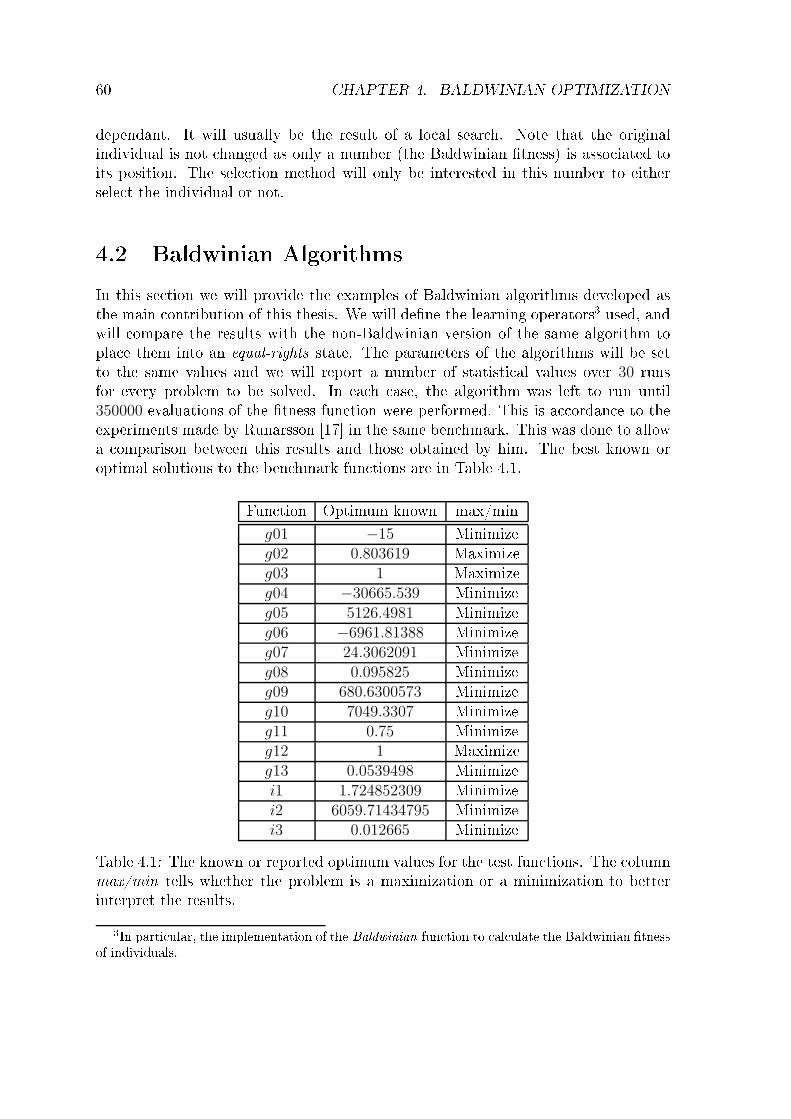
60 CHAPTER 4. BALDWINIAN OPTIMIZATIONdependant. It will usually be the result of a lo al sear h. Note that the originalindividual is not hanged as only a number (the Baldwinian tness) is asso iated toits position. The sele tion method will only be interested in this number to eithersele t the individual or not.4.2 Baldwinian AlgorithmsIn this se tion we will provide the examples of Baldwinian algorithms developed asthe main ontribution of this thesis. We will dene the learning operators3 used, andwill ompare the results with the non-Baldwinian version of the same algorithm topla e them into an equal-rights state. The parameters of the algorithms will be setto the same values and we will report a number of statisti al values over 30 runsfor every problem to be solved. In ea h ase, the algorithm was left to run until350000 evaluations of the tness fun tion were performed. This is a ordan e to theexperiments made by Runarsson [17 in the same ben hmark. This was done to allowa omparison between this results and those obtained by him. The best known oroptimal solutions to the ben hmark fun tions are in Table 4.1.Fun tion Optimum known max/min

g01 −15 Minimizeg02 0.803619 Maximizeg03 1 Maximizeg04 −30665.539 Minimizeg05 5126.4981 Minimizeg06 −6961.81388 Minimizeg07 24.3062091 Minimizeg08 0.095825 Minimizeg09 680.6300573 Minimizeg10 7049.3307 Minimizeg11 0.75 Minimizeg12 1 Maximizeg13 0.0539498 Minimizei1 1.724852309 Minimizei2 6059.71434795 Minimizei3 0.012665 MinimizeTable 4.1: The known or reported optimum values for the test fun tions. The olumnmax/min tells whether the problem is a maximization or a minimization to betterinterpret the results.3In parti ular, the implementation of the Baldwinian fun tion to al ulate the Baldwinian tnessof individuals.

4.2. BALDWINIAN ALGORITHMS 61The test fun tions are of onstrained optimization, and they an be found inthe appendix. For a detailed explanation on the fun tions, the reader should he k[17, 13.4.2.1 Baldwinian evolutionary strategyThe lassi al evolutionary strategy ES(µ, λ) with self-adaptation parameters (σi),reviewed in Se tion 2.3, with a te hnique of rules with total sum of violations seen inSe tion 1.3.2.2 will be used.The genotype will be augmented with the values of strength, so that it will bep = (x1, x2, . . . , xl; σ1, σ2, . . . , σl; s1, s2, . . . , sl)where 0 ≤ si ≤ 1 for every 1 ≤ i ≤ l, and they represent the strength of instin t inthe obje tive i. We will use ~x = (x1, x2, . . . , xl) to denote the obje tive portion of thegenotype, ~σ = (σ1, σ2, . . . , σl) to denote the ontrol portion, and ~s = (s1, s2, . . . , sl)to denote the strength portion.This new evolution strategy will be ompared with the strategy dis ussed in Se -tion 2.3.4, and it will have the same parameter setting, ex ept for the added strengthportion.The idea behind the learning operator is to use the same lo al sear h introdu edby the σ's in the learning step. This is to avoid the appearan e of unne essaryparameters in the algorithm.The rossover operator used in the obje tive values will be intermediate-generalized,while in the ontrol values and strengths will be dis rete (see Se tion 2.3.3). The mu-tation will be as usual for the self-adaptive evolutionary strategy for obje tive and ontrol values, and the strength will be mutated as followssm

i = max0,minsi + Normal(0, 1), 1i.e. the strength will be added a standard normal value, ropped to [0, 1]. Thefun tionρ(x) =

n∑

i=1

g+i (x) +

m∑

i=1

h+j (x)represents the total sum of violations of x ∈ S, with all the weights equal to 1.In order to al ulate the Baldwinian tness value of an individual, we will use thefollowing algorithmBaldwinian tness

~xB = ~x;for( i = 1 to l )if( si <rand() )

62 CHAPTER 4. BALDWINIAN OPTIMIZATION~x− = ~xB − (0, 0, . . . , σi, . . . , 0); //at the i-th position.~x+ = ~xB +(0, 0, . . . , σi, . . . , 0); //at the i-th position.~xB = arg minρ τ(~xB), ρ τ(~x−), ρ τ(~x+);setFitness( ~x, f τ(~xB) );As we an observe, the learning an take pla e in every obje tive value, or in none.It all depends on the values of the learning strength. Here, in ontrast to Turney, weare not interested in the evolutionary pro ess ae ting the strengths, or whether thestrengths follow the path predi ted by the Baldwin Ee t; that is left for a future work.Instead we are interested in whether this Baldwinian learning aids the optimizationpro ess or not.Statisti value Normal ES(µ+ λ) Baldwinian ES(µ+ λ)best 14.999983 15.643469worst 12.884572 13.029993mean 14.524280 15.0092431median 14.999897 15.296720varian e 0.564467 0.404876standard deviation 0.751310 0.636299# feasibles 30 21*# ǫ-feasibles 30 30Table 4.2: Results for fun tion g01Statisti value Normal ES(µ+ λ) Baldwinian ES(µ+ λ)best 0.403915 0.416605worst 0.295487 0.284842mean 0.360394 0.358947median 0.366991 0.3610752varian e 6.5839E-4 0.001052standard deviation 0.025659 0.032445# feasibles 30 13*# ǫ-feasibles 30 30Table 4.3: Results for fun tion g02The results for the ben hmark fun tions are summarized in Tables 4.24.14. Theresults for the engineering problems are in Tables 4.154.17.It is important to explain the apparently lower number of true feasible solutionfound by the algorithms. First of all, when the problem has equality onstraints, itis impossible, due to a dis retization error, to a hieve the a tual equality. Instead,every solution is ǫ-feasible, with an ǫ ∼ 10−5. For the rest of the problems, the status

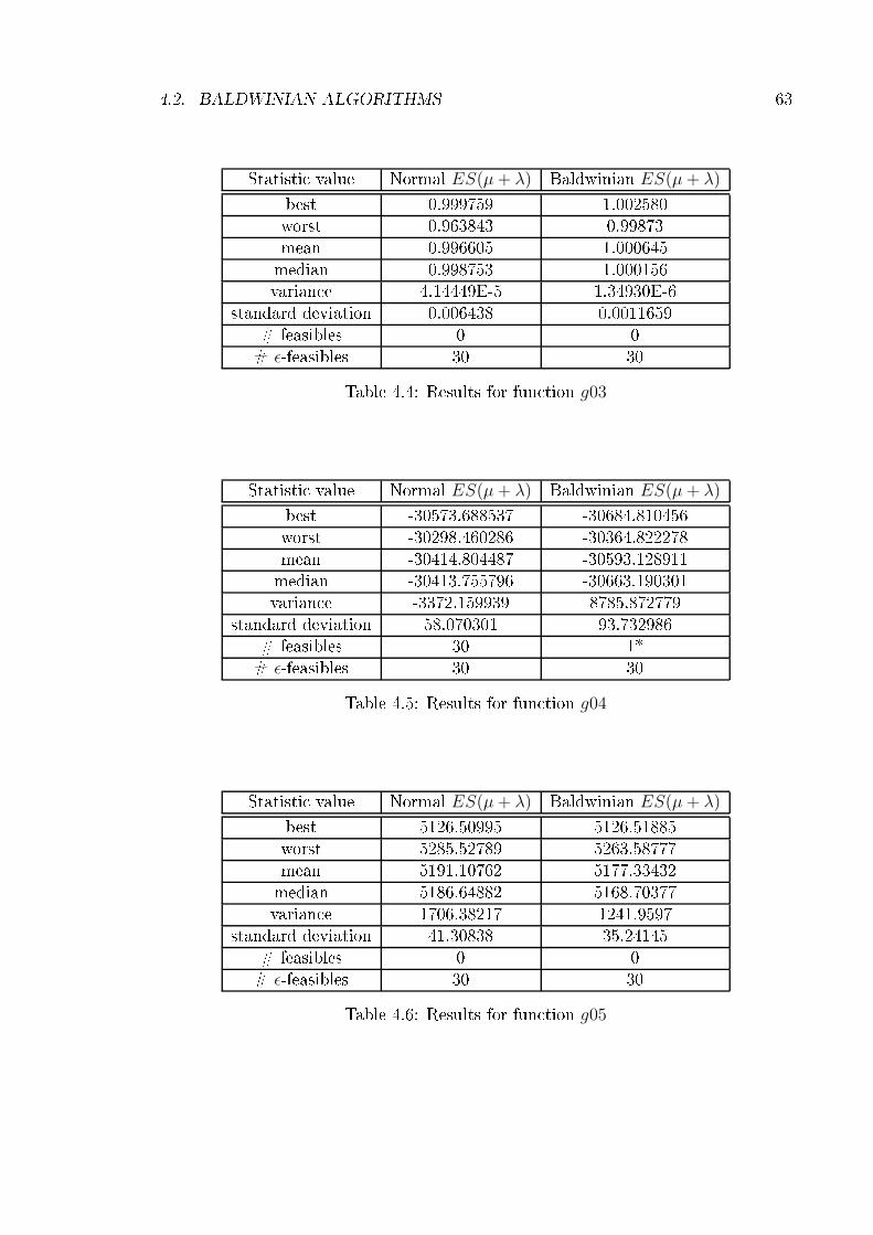
4.2. BALDWINIAN ALGORITHMS 63Statisti value Normal ES(µ+ λ) Baldwinian ES(µ+ λ)best 0.999759 1.002580worst 0.963843 0.99873mean 0.996605 1.000645median 0.998753 1.000156varian e 4.14449E-5 1.34930E-6standard deviation 0.006438 0.0011659# feasibles 0 0# ǫ-feasibles 30 30Table 4.4: Results for fun tion g03

Statisti value Normal ES(µ+ λ) Baldwinian ES(µ+ λ)best -30573.688537 -30684.810456worst -30298.460286 -30364.822278mean -30414.804487 -30593.128911median -30413.755796 -30663.190301varian e -3372.159939 8785.872779standard deviation 58.070301 93.732986# feasibles 30 1*# ǫ-feasibles 30 30Table 4.5: Results for fun tion g04

Statisti value Normal ES(µ+ λ) Baldwinian ES(µ+ λ)best 5126.50995 5126.51885worst 5285.52789 5263.58777mean 5191.10762 5177.33432median 5186.64882 5168.70377varian e 1706.38217 1241.9597standard deviation 41.30838 35.24145# feasibles 0 0# ǫ-feasibles 30 30Table 4.6: Results for fun tion g05

64 CHAPTER 4. BALDWINIAN OPTIMIZATIONStatisti value Normal ES(µ+ λ) Baldwinian ES(µ+ λ)best -6961.81382 -6961.816175worst -1206.19807 -6961.813383mean -6576.84885 -6961.813834median -6961.21074 -6961.813767varian e 2046571.365351 2.36233E-7standard deviation 1430.58427 4.86038E-4# feasibles 30 13*# ǫ-feasibles 30 30Table 4.7: Results for fun tion g06

Statisti value Normal ES(µ+ λ) Baldwinian ES(µ+ λ)best 24.876975 24.584865worst 28.592849 29.549636mean 26.196125 25.654459median 25.924144 25.163657varian e 0.866379 1.233E-7standard deviation 0.930795 1.110668# feasibles 30 14*# ǫ-feasibles 30 30Table 4.8: Results for fun tion g07

Statisti value Normal ES(µ+ λ) Baldwinian ES(µ+ λ)best 0.095825 0.095825worst 0.004505 0.013637mean 0.068281 0.059710median 0.095825 0.065143varian e 0.001185 0.001188standard deviation 0.034431 0.034478# feasibles 30 30# ǫ-feasibles 30 30Table 4.9: Results for fun tion g08

4.2. BALDWINIAN ALGORITHMS 65Statisti value Normal ES(µ+ λ) Baldwinian ES(µ+ λ)best 680.656456 677.608343worst 685.906514 680.676598mean 681.738274 680.465658median 681.149711 680.636904varian e 1.4761804 0.3083865standard deviation 1.2149816 0.555325# feasibles 30 4*# ǫ-feasibles 30 30Table 4.10: Results for fun tion g09

Statisti value Normal ES(µ+ λ) Baldwinian ES(µ+ λ)best 14743.296345 12903.07097worst 20334.78599 19457.0973mean 16775.12296 16503.5519median 16668.745345 16354.4338varian e 1094703.55833 2162402.151standard deviation 1046.280821 1470.5108# feasibles 1 2*# ǫ-feasibles 30 30Table 4.11: Results for fun tion g10

Statisti value Normal ES(µ+ λ) Baldwinian ES(µ+ λ)best 0.749955 0.731125worst 0.751152 0.750204mean 0.750309 0.743945median 0.750214 0.747179varian e 8.3655E-8 4.5196E-5standard deviation 2.8923E-4 0.006723# feasibles 0 0# ǫ-feasibles 30 30Table 4.12: Results for fun tion g11

66 CHAPTER 4. BALDWINIAN OPTIMIZATIONStatisti value Normal ES(µ+ λ) Baldwinian ES(µ+ λ)best 1.0 1.0worst 0.939999 0.9699999mean 0.986333 0.9903333median 0.99000 0.990000varian e 1.2322E-4 6.9888E-5standard deviation 0.011100 0.008359# feasibles 30 30# ǫ-feasibles 30 30Table 4.13: Results for fun tion g12

Statisti value Normal ES(µ+ λ) Baldwinian ES(µ+ λ)best 0.624860 0.4664885worst 0.99990 0.9999465mean 0.91796 0.8497140median 0.989343 0.899186varian e 0.013152 0.017600standard deviation 0.114683 0.132667# feasibles 0 0# ǫ-feasibles 30 30Table 4.14: Results for fun tion g13

Statisti value Normal ES(µ+ λ) Baldwinian ES(µ+ λ)best 1.836054 1.724852worst 2.384537 2.574196mean 2.050582 1.974465median 2.006084 1.924799varian e 0.016603 0.03675standard deviation 0.128856 0.19172# feasibles 30 15*# ǫ-feasibles 30 30Table 4.15: Results for fun tion i1

4.2. BALDWINIAN ALGORITHMS 67Statisti value Normal ES(µ+ λ) Baldwinian ES(µ+ λ)best 6488.3890 6890.85390worst 16783.24940 13053.0751mean 10811.4691 10113.5241median 10796.35730 9850.33251varian e 4984724.191 3011815.7516standard deviation 2232.6495 1735.4583# feasibles 30 13*# ǫ-feasibles 30 30Table 4.16: Results for fun tion i2

Statisti value Normal ES(µ+ λ) Baldwinian ES(µ+ λ)best 0.012704 0.0124919worst 0.013231 0.0130756mean 0.012875 0.0128605median 0.012838 0.0128425varian e 1.5581E-8 1.3777E-8standard deviation 1.2482E-4 1.1737E-4# feasibles 30 20*# ǫ-feasibles 30 30Table 4.17: Results for fun tion i3

68 CHAPTER 4. BALDWINIAN OPTIMIZATIONof ǫ-feasible is hanging; it is about 10−6 times the maximum a hieved absolute valueof the tness fun tion.In the ending, it might seem that the Baldwinian algorithm fails to rea h feasiblesolution in almost every problem, but this is just a misinterpretation of the results.As the best individual is often one who has learned (i.e. has an in reased tness valuedue to learning), but the genotype remains un hanged, it is fairly di ult to knowfor sure what is its Baldwinian violation by just looking at the genes. The numberspresented in the tables are only the individual's geneti al violations, not the a tualbest violations. In order to obtain that value of tness, the individual had a violationof ee tively 0 after learning, making him feasible in its Baldwinian value4.Under the light shed by the last observation, we are safe to assure that the Bald-winian version of the algorithm outperforms, in general, the non-Baldwinian version.And a tually, it performed fairly well for su h a simple algorithm used on well-knowndi ult optimization problems.In the next se tion we will introdu e a Baldwinian version of a more powerfulevolutionary algorithm.4.2.2 Baldwinian Dierential EvolutionThe dierential evolution algorithm DE_1(CR,F ) reviewed in Se tion 2.5 , with ate hnique of rules with total sum of violations seen in Se tion 1.3.2.2 will be used.The genotype will be augmented with the value of strength, so that it will bep = (x1, x2, . . . , xl; s)where 0 ≤ s ≤ 1, and it represents the strength of instin t. If the individual isto learn, it will have MAX attempts to improve its onstraint ve tor from a lo alvariation on the F parameter. Usually, the value of MAX is set to 2, but varioustries pointed to the good robustness of this parameter.This new dierential evolution will be ompared with the dierential evolutiondis ussed in Se tion 2.5.4, and it will have the same parameter setting, ex ept for theadded strength portion.The idea behind the learning operator is to use the lo al sear h with the parameter

F in the learning step, as a solution with values near the produ ed individual is likelyto have similar values in the dieren e part of the pro ess.As in the last se tion, we will use ~x = (x1, x2, . . . , xl) to denote the obje tiveportion of the genotype.The rossover operator used is the same than in the normal algorithm. Thestrength of the reated ve tor will be set to the parent's value, plus a normal randomnumber with standard deviation 0.1, with a probability of C, otherwise it is set to0.9s. The value of C an be used to ontrol the in reasing ratio of the strength.The reation of a new individual hanges a bit in this algorithm, but it is essentiallythe same as the original dierential evolution. Assume we are reating the ospring4That is the reason for the asterisk at the tables' # feasibles row.

4.2. BALDWINIAN ALGORITHMS 69of individual i in the population P , i.e. ~x is the obje tive part of the individual pi,and s is the strength part.Baldwinian omparison~xoff = reateOffspring(F);~xB = ~xoff;if( s <rand() )for( i = 1 to MAX )

~xtemp = reateOffspring(F+Normal(0,0.1);if( ρ τ(~xB) > ρ τ(~xtemp) )~xB = ~xtemp;if(better( ~xB, ~x ))if( 0.9 <rand() )

pnext,i =( ~xoff, 0.9s );elsepnext,i =( ~xoff, rand() );else

pnext,i = pi;As we an observe, the learning an take pla e MAX times or 0 times. As with the ase of the evolutionary strategy, it depends on the values of the learning strength.Again, the individual is not modied; observe that the ospring ~xoff is assigned tothe next generation if the Baldwinian individual is better than the parent individual'spart ~x. Statisti value Normal DE(0.9, 0.9) Baldwinian DE(0.9, 0.9)best -15 -15worst -15 -15mean -15 -15median -15 -15varian e 0 0standard deviation 0 0# feasibles 30 30# ǫ-feasibles 30 30Table 4.18: Results for fun tion g01The results for the ben hmark fun tions are summarized in Tables 4.184.30, andthe results for the engineering problems are in Tables 4.314.33.

70 CHAPTER 4. BALDWINIAN OPTIMIZATIONStatisti value Normal DE(0.9, 0.9) Baldwinian DE(0.9, 0.9)best 0.8036189 0.8036189worst 0.8029367 0.8014754mean 0.8035043 0.8032154median 0.8036163 0.8036028varian e 3.45886E-8 3.67254E-7standard deviation 1.8598E-4 6.06014E-4# feasibles 30 30# ǫ-feasibles 30 30Table 4.19: Results for fun tion g02

Statisti value Normal DE(0.9, 0.9) Baldwinian DE(0.9, 0.9)best 1 1worst 0.9999873 0.9998754mean 0.9999990 0.9999846median 0.9999999 0.9999998varian e 5.47056E-12 1.0087E-9standard deviation 2.33892E-6 3.17606E-5# feasibles 0 0# ǫ-feasibles 30 30Table 4.20: Results for fun tion g03

Statisti value Normal DE(0.9, 0.9) Baldwinian DE(0.9, 0.9)best 30665.538671 30665.538671worst 30665.538671 30665.538671mean 30665.538671 30665.538671median 30665.538671 30665.538671varian e 1.2837E-22 1.4999E-22standard deviation 1.1330E-11 1.2247E-11# feasibles 30 30# ǫ-feasibles 30 30Table 4.21: Results for fun tion g04

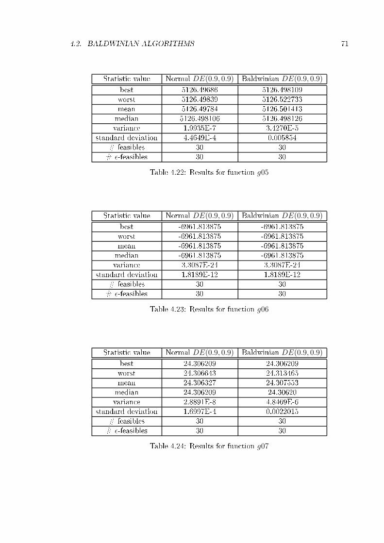
4.2. BALDWINIAN ALGORITHMS 71Statisti value Normal DE(0.9, 0.9) Baldwinian DE(0.9, 0.9)best 5126.49686 5126.498109worst 5126.49839 5126.522733mean 5126.49784 5126.501413median 5126.498106 5126.498126varian e 1.9935E-7 3.4270E-5standard deviation 4.4649E-4 0.005854# feasibles 30 30# ǫ-feasibles 30 30Table 4.22: Results for fun tion g05

Statisti value Normal DE(0.9, 0.9) Baldwinian DE(0.9, 0.9)best -6961.813875 -6961.813875worst -6961.813875 -6961.813875mean -6961.813875 -6961.813875median -6961.813875 -6961.813875varian e 3.3087E-24 3.3087E-24standard deviation 1.8189E-12 1.8189E-12# feasibles 30 30# ǫ-feasibles 30 30Table 4.23: Results for fun tion g06

Statisti value Normal DE(0.9, 0.9) Baldwinian DE(0.9, 0.9)best 24.306209 24.306209worst 24.306643 24.313465mean 24.306327 24.307553median 24.306209 24.30620varian e 2.8891E-8 4.8469E-6standard deviation 1.6997E-4 0.0022015# feasibles 30 30# ǫ-feasibles 30 30Table 4.24: Results for fun tion g07

72 CHAPTER 4. BALDWINIAN OPTIMIZATIONStatisti value Normal DE(0.9, 0.9) Baldwinian DE(0.9, 0.9)best 0.09582 0.095825worst 0.09582 0.095825mean 0.09582 0.095825median 0.09582 0.095825varian e 5.6493E-34 4.0445E-34standard deviation 2.3768E-17 2.0110E-17# feasibles 30 30# ǫ-feasibles 30 30Table 4.25: Results for fun tion g08

Statisti value Normal DE(0.9, 0.9) Baldwinian DE(0.9, 0.9)best 680.630057 680.630057worst 680.630057 680.630057mean 680.630057 680.630057median 680.630057 680.630057varian e 1.7879E-25 2.4987E-25standard deviation 4.2283E-13 4.9987E-13# feasibles 30 30# ǫ-feasibles 30 30Table 4.26: Results for fun tion g09

Statisti value Normal DE(0.9, 0.9) Baldwinian DE(0.9, 0.9)best 7049.248020 7049.248020worst 7049.260829 7049.359981mean 7049.250584 7049.270574median 7049.248020 7049.24802varian e 1.6376E-5 2.29355E-4standard deviation 0.004046 0.01514# feasibles 30 30# ǫ-feasibles 30 30Table 4.27: Results for fun tion g10

4.2. BALDWINIAN ALGORITHMS 73Statisti value Normal DE(0.9, 0.9) Baldwinian DE(0.9, 0.9)best 0.749904 0.750000worst 0.750028 0.750813mean 0.749982 0.750163median 0.749999 0.750001varian e 1.1238E-9 6.0038E-8standard deviation 3.3524E-5 2.4502E-4# feasibles 0 0# ǫ-feasibles 30 30Table 4.28: Results for fun tion g11

Statisti value Normal DE(0.9, 0.9) Baldwinian DE(0.9, 0.9)best 0.98 1.0worst 0.59 0.520018mean 0.852052 0.775251median 0.865 0.784590varian e 0.007546 0.012312standard deviation 0.086868 0.110963# feasibles 30 30# ǫ-feasibles 30 30Table 4.29: Results for fun tion g12

Statisti value Normal DE(0.9, 0.9) Baldwinian DE(0.9, 0.9)best 0.053943 0.053949worst 0.438851 0.73930mean 0.272058 0.35564median 0.438829 0.43885varian e 0.036378 0.034533standard deviation 0.190731 0.18583# feasibles 30 30# ǫ-feasibles 30 30Table 4.30: Results for fun tion g13

74 CHAPTER 4. BALDWINIAN OPTIMIZATIONStatisti value Normal DE(0.9, 0.9) Baldwinian DE(0.9, 0.9)best 1.724852 1.724852worst 1.724852 1.724852mean 1.724852 1.724852median 1.724852 1.724852varian e 1.2325E-30 1.2325E-30standard deviation 1.1102E-15 1.1102E-15# feasibles 30 30# ǫ-feasibles 30 30Table 4.31: Results for fun tion i1Statisti value Normal DE(0.9, 0.9) Baldwinian DE(0.9, 0.9)best 6059.774753 6059.774753worst 6059.774753 6059.775651mean 6059.774753 6059.77481median 6059.774753 6059.77475varian e 3.3087E-24 2.9341E-8standard deviation 1.8189E-12 1.7129E-4# feasibles 30 30# ǫ-feasibles 30 30Table 4.32: Results for fun tion i2Statisti value Normal DE(0.9, 0.9) Baldwinian DE(0.9, 0.9)best 0.012665 0.012665worst 0.012665 0.012665mean 0.012665 0.012665median 0.012665 0.012665varian e 3.5910E-35 3.3202E-35standard deviation 5.9925E-18 5.7621E-18# feasibles 30 30# ǫ-feasibles 30 30Table 4.33: Results for fun tion i3

4.3. CONCLUSIONS ON THE EXPERIMENTS 754.3 Con lusions on the ExperimentsAs we might see in the tables, the performan e of the Baldwinian version of well-known optimization algorithms is fairly better or equal than the non-Baldwinian ounterpart. As expe ted, the varian e is greater, but the best value is usually betteror equal to the one obtained by the normal version.Our main observation in the tables is that, when the problem is a di ult one,the Baldwinian version outperforms, on average, the normal version of the algorithm;whereas this means that the Baldwinian algorithm is better5 than the normal one ornot remains unknown as the varian e is usually greater in the Baldwinian ase. Atleast this behavior proves what we expe ted from the observations on the BaldwinEe t in Chapter 3.The learning operator for both ases is very simple as it was only used to illustratethe ee ts that learning an have on evolution. Better learning operators will lead tobetter results, but, as the Baldwin Ee t tea hes us, we must exer ise aution whenusing learning be ause the omputation time expend in learning is time lost fromevolution.All the experiments performed until now studied the Baldwinian algorithms to seewhether the Baldwin Ee t was present or not in the evolutionlearning intera tions.What we wanted to measure was the strengths of Baldwinian Algorithms, and if theyare worth the try.In order to see a full Baldwinian behavior on evolutionary algorithms, a hugeamount of omputational power was spent in order to better understand its ee ts.As we an see in the experiments performed by Hinton, Nowlan, Belew and Turney,the longer we let the algorithm run, the better the results we obtain are.In ontrast, we wanted to see if Baldwinian optimization an be applied to aproblem with limited omputational resour es (as are 350000 evaluations of the t-ness fun tion) and still su eed in the optimization pro ess by obtaining respe tablesolutions.

5In the sense of statisti al robustness and behavior.

76 CHAPTER 4. BALDWINIAN OPTIMIZATION

Con lusionsIt is undeniable that more and more resear hers are being attra ted by the oeringsof new hybridization te hniques. Nature has always been a sour e of inspiration toman-kind, and we an learly see this in the development of biologi ally inspiredalgorithms.The Baldwin Ee t might be a not-well-understood for e in evolution, or an bejust a biologi al uriosity. Either ase, we an exploit it to be of use to evolutionary omputation. Early experiments pointed to the strength of learning by solving prob-lems of the type needle in a hay sta k whi h are well known di ult optimizationproblems. The at h seems to be in learning and the way it was implemented. Learn-ing is ostly, and the experiments were more on erned with idealized algorithms withvirtually unlimited omputation resour es.In this thesis we wanted to issue the performan e problem derived from learning.We ompared the algorithm Baldwinian algorithm with the non-Baldwinian versionof it, and the results are presented. Whether the Baldwinian version is better ornot is something that we are not dire tly interested in. Instead we wanted to verifyif it was possible to reate a ompetitive algorithm based on the on epts from theBaldwin Ee t.Fortunately, most results were expe ted, and the issue of better is not easy toaddress with high varian e results as obtained. However, learning was expe ted to in- rease the varian e of results, and in general, the Baldwinian algorithm demonstratedan ex ellent better result, fairly good mean and median, and slightly large standarddeviation.We see the Baldwinian algorithms as a promising area of resear h, and expe t theideas to spread in the omputing ommunity. A good example of this an be seenin the birth of memeti algorithms, whi h resemble Baldwinian ones to the point inwhi h many people even think they are the same.In addition, if the on epts of Lamar kism have been used as valid omputer mod-els (although not biologi ally a urate) for optimization, using Baldwinian models is ertainly as valid as Lamar kian. In the end, we an exploit more the Baldwinian on- epts as are sus eptible to be further studied in biology and, in onsequen e, betterunderstood by omputer s ientists.77

78 CHAPTER 4. BALDWINIAN OPTIMIZATION

Bibliography[1 Bä k. T., Hammel, U. and S hwefel, H.-P., (1997). Evolutionary Computation: omments on the history and urrent state. IEEE Trans. on Evo. Comp. 1 (1):3-17.[2 Baldwin, J. M. (1896). A new fa tor in evolution. Ameri an Naturalist 30: 441-451, 536-553.[3 Belew, R. K. (1990). Evolution, learning and ulture. Computational metaphorsfor adaptive algorithms. Complex Systems 4 : 11-49.[4 Bu kles, B. P., Coello, C. A. and Hernández, A. (1998). Estrategias evoluti-vas: La versión alemana del algoritmo genéti o. (I & II). Solu iones Avanzadas.Te nologías de Informa ión y Estrategias de Nego ios. Año 6, (62), 38-45.[5 Coello, C. and Mezura, E. (2004). What makes a onstrained optimization prob-lem di ult to solve. Evolutionary Computation Group at CINVESTAV, D.F.,Mexi o.[6 Dawkins, R. (1976). The selsh gene. Oxford: Oxford University Press.[7 Eiben, A. E. and Smith, J. E., (2003), Introdu tion to evolutionary omputing.Natural omputing series. Springer. (10): 173-180.[8 Fogel, L. J., (1962). Autonomous automata, Industrial Resear h 4: 14-19.[9 Harvey, I. (1993). The puzzle of the persistent question marks: A ase study ofgeneti drift. Pro eedings of the 5th International Conferen e on GA. MorganKaufmann[10 Hinton, G. E., and Nowlan, S. J. (1987). How learning an guide evolution.Complex Systems, 1, 495-502.[11 Holland, J. H., (1975). Adaptation in natural and arti ial systems. The Univer-sity of Mi higan Press, Ann Abor, MI.[12 Koza, J. R., (1992). Geneti Programming: On the programming of omputersby means of natural sele tion. MIT Press.79

80 BIBLIOGRAPHY[13 Koziel, S., and Mi halewi z, Z., (1999). Evolutionary algorithms, homomorphousmappings, and onstrained parameter optimization. Evolutionary Computation,7(1), 19-44.[14 Mit hell, M. (1998). An introdu tion to Geneti Algorithms. The MIT Press (3),87-95.[15 Pri e, K. and Storn, R. (1996). Dierential evolution - A simple and e ientadaptive s heme for global optimization over ontinuous spa es. Te hni al ReportTR-95-012, ICSI.[16 Re henberg, I., (1965). Cyberneti solution path of an experimental problem.Journal of the ACM 3, 297-314.[17 Runarsson, T. P., and Yao, X. (2000). Sto hasti Ranking for onstrained evo-lutionary optimization. IEEE Trans. on Evo. Comp., TEC#311R.[18 S hwefel, H.-P., (1968). Projekt MHD-Staustrahlrohr: Experimentelle Opti-mierung einer Zweiphasenädse, Teil I. Te hnis her Beri ht 11.034/68, 35.[19 Simpson, G. G. (1956). The Baldwin Ee t. Evolution 7, 110-117.[20 Turney, P. (1996). Myths and legends of the Baldwin Ee t. Evo. Comp. andMa hine Learning (ICML-96), 135-142. NRC-39220.[21 Turney, P. (1996). How to shift Bias: Lessons from the Baldwin Ee t. NationalResear h Coun il Canada, Institute for IT. K1A 0R6.[22 Waddington, C. H. (1942). Canalization of development and the inheritan e ofa quired hara ters. Nature 150, 563-565.

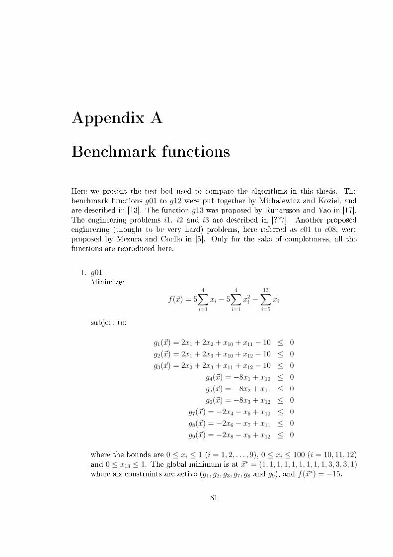
Appendix ABen hmark fun tionsHere we present the test bed used to ompare the algorithms in this thesis. Theben hmark fun tions g01 to g12 were put together by Mi halewi z and Koziel, andare des ribed in [13. The fun tion g13 was proposed by Runarsson and Yao in [17.The engineering problems i1, i2 and i3 are des ribed in [???. Another proposedengineering (thought to be very hard) problems, here referred as c01 to c08, wereproposed by Mezura and Coello in [5. Only for the sake of ompleteness, all thefun tions are reprodu ed here.1. g01Minimize:f(~x) = 5

4∑

i=1

xi − 54∑

i=1

x2i −

13∑

i=5

xisubje t to:g1(~x) = 2x1 + 2x2 + x10 + x11 − 10 ≤ 0

g2(~x) = 2x1 + 2x3 + x10 + x12 − 10 ≤ 0

g3(~x) = 2x2 + 2x3 + x11 + x12 − 10 ≤ 0

g4(~x) = −8x1 + x10 ≤ 0

g5(~x) = −8x2 + x11 ≤ 0

g6(~x) = −8x3 + x12 ≤ 0

g7(~x) = −2x4 − x5 + x10 ≤ 0

g8(~x) = −2x6 − x7 + x11 ≤ 0

g9(~x) = −2x8 − x9 + x12 ≤ 0where the bounds are 0 ≤ xi ≤ 1 (i = 1, 2, . . . , 9), 0 ≤ xi ≤ 100 (i = 10, 11, 12)and 0 ≤ x13 ≤ 1. The global minimum is at ~x∗ = (1, 1, 1, 1, 1, 1, 1, 1, 1, 3, 3, 3, 1)where six onstraints are a tive (g1, g2, g3, g7, g8 and g9), and f(~x∗) = −15.81

82 APPENDIX A. BENCHMARK FUNCTIONS2. g02Maximize:f(~x) =

∣

∣

∣

∣

∣

∑ni=1 cos4(xi) − 2

∏ni=1 cos2(xi)

√

∑ni=1 ix

2i

∣

∣

∣

∣

∣subje t to:g1(~x) = 0.75 −

n∏

i=1

xi ≤ 0

g2(~x) =n∑

i=1

xi − 7.5n ≤ 0where n = 20, the bounds are 0 ≤ xi ≤ 10 (i = 1, 2, . . . , n). The global mini-mum is unknown, the best found reported previously is f(~x) = 0.803619, with~x∗ =(3.171456, 3.175499, 3.121430, 3.065424, 3.024695, 2.985945, 2.956863,2.880306, 0.506161, 0.509743, 0.486445, 0.481882, 0.487077, 0.459685, 0.467321,0.445682, 0.439956, 0.444745, 0.431957, 0.424569) with the onstraint g02 being lose to a tive.3. g03Maximize:

f(~x) = (√n)n

n∏

i=1

xisubje t to:h1(~x) =

n∑

i=1

x2i − 1 = 0where n = 10 and the bounds are 0 ≤ xi ≤ 1 (i = 1, 2, . . . , n). The globalmaximum is at x∗i = 1/

√n (i = 1, 2, . . . , n) where f(~x∗) = 1.4. g04Minimize:

f(~x) = 5.3578547x23 + 0.8356891x1x5 + 37.293239x1 − 40792.141subje t to:

g1(~x) = 85.334407 + 0.0056858x2x5 + 0.0006262x1x4

−0.0022053x3x5 − 92 ≤ 0

g2(~x) = −85.334407 − 0.0056858x2x5 − 0.0006262x1x4

+0.0022053x3x5 ≤ 0

g3(~x) = 80.51249 + 0.0071317x2x5 + 0.0029955x1x2

83+0.0021813x2

3 − 110 ≤ 0

g4(~x) = −80.51249 − 0.0071317x2x5 − 0.0029955x1x2

−0.0021813x23 + 90 ≤ 0

g5(~x) = 9.300961 + 0.0047026x3x5 + 0.0012547x1x3

+0.0019085x3x4 − 25 ≤ 0

g6(~x) = −9.300961 − 0.0047026x3x5 − 0.0012547x1x3

−0.0019085x3x4 + 20 ≤ 0where the bounds are 78 ≤ x1 ≤ 102, 33 ≤ x2 ≤ 45, and 27 ≤ xi ≤ 45(i = 3, 4, 5). The best solution is ~x∗ = (78, 33, 29.995256, 45, 36.775813) wheref(~x∗) = −30665.539. Two onstraints are a tive (g1 and g6).5. g05Minimize:

f(~x) = 3x1 + 0.000001x31 + 2x2 + (0.000002/3)x3

2subje t to:g1(~x) = −x4 + x3 − 0.55 ≤ 0

g2(~x) = −x3 + x4 − 0.55 ≤ 0

h3(~x) = 1000 sin(−x3 − 0.25) + 1000 sin(−x4 − 0.25) + 894.8 − x1 = 0

h4(~x) = 1000 sin(x3 − 0.25) + 1000 sin(x3 − x4 − 0.25) + 894.8 − x2 = 0

h5(~x) = 1000 sin(x4 − 0.25) + 1000 sin(x4 − x3 − 0.25) + 1294.8 = 0where the bounds are 0 ≤ x1 ≤ 1200, 0 ≤ x2 ≤ 1200, −0.55 ≤ x3 ≤ 0.55,and −0.55 ≤ x4 ≤ 0.55. The best known solution is ~x∗ = (679.9453, 1026.067,0.118876, −0.396234) where two onstraints are a tive (g1 and g6), and f(~x∗) =5126.4981.6. g06Minimize:

f(~x) = (x1 − 10)3 + (x2 − 20)3subje t to:g1(~x) = −(x1 − 5)2 − (x2 − 5)2 + 100 ≤ 0

g2(~x) = −(x1 − 6)2 + (x2 − 5)2 − 82.81 ≤ 0where the bounds are 13 ≤ x1 ≤ 100 and 0 ≤ x2 ≤ 100. The optimumsolution is ~x∗ = (14.095, 0.84296)where both onstraints are a tive, and f(~x∗) =−6961.81388.7. g07Minimize:f(~x) = x2

1 + x22 + x1x2 − 14x1 − 16x2 + (x3 − 10)2 + 4(x4 − 5)2 + (x5 − 3)2

+2(x6 − 1)2 + 5x27 + 7(x8 − 11)2 + 2(x9 − 10)2 + (x10 − 7)2 + 45

84 APPENDIX A. BENCHMARK FUNCTIONSsubje t to:g1(~x) = −105 + 4x1 + 5x2 − 3x7 + 9x8 ≤ 0

g2(~x) = 10x1 − 8x2 − 17x7 + 2x8 ≤ 0

g3(~x) = −8x1 + 2x2 + 5x9 − 2x10 − 12 ≤ 0

g4(~x) = 3(x1 − 2)2 + 4(x2 − 3)2 + 2x23 − 7x4 − 120 ≤ 0

g5(~x) = 5x21 + 8x2 + (x3 − 6)2 − 2x4 − 40 ≤ 0

g6(~x) = x21 + 2(x2 − 2)2 − 2x1x2 + 14x5 − 6x6 ≤ 0

g7(~x) = 0.5(x1 − 8)2 + 2(x2 − 4)2 + 3x25 − x6 − 30 ≤ 0

g8(~x) = −3x1 + 6x2 + 12(x9 − 8)2 − 7x10 ≤ 0where the bounds are −10 ≤ xi ≤ 10 (i = 1, 2, . . . , 10). The optimum solutionis ~x∗ =(2.171996, 2.363683, 8.773926, 5.095984, 0.9906548, 1.430574, 1.321644,9.828726, 8.280092, 8.375927) where six onstraints are a tive (g1, g2, g3, g4, g5and g6), and f(~x∗) = 24.3062091.8. g08Minimize:

f(~x) =sin3(2πx1) sin(2πx2)

x31(x1 + x2)subje t to:

g1(~x) = x21 − x2 + 1 ≤ 0

g2(~x) = 1 − x1 + (x2 − 4)2 ≤ 0where the bounds are 0 ≤ x1 ≤ 10 and 0 ≤ x2 ≤ 10. The optimum is at~x∗ = (1.2279713, 4.2453733) where f(~x∗) = 0.095825.9. g09Minimize:

f(~x) = (x1 − 10)2 + 5(x2 − 12)2 + x43 + 3(x4 − 11)2

+10x65 + 7x2

6 + x47 − 4x6x7 − 10x6 − 8x7subje t to:

g1(~x) = −127 + 2x21 + 3x4

2 + x3 + 4x24 + 5x5 ≤ 0

g2(~x) = −282 + 7x1 + 3x2 + 10x23 + x4 − x5 ≤ 0

g3(~x) = −196 + 23x1 + x22 + 6x2

6 − 8x7 ≤ 0

g4(~x) = 4x21 + x2

2 − 3x1x2 + 2x23 + 5x6 − 11x7 ≤ 0where the bounds are −10 ≤ xi ≤ 10 (i = 1, 2, . . . , 7). The optimum solutionis at ~x∗ =(2.330499, 1.951372, −0.4775414, 4.365726, −0.6244870, 1.038131,

1.594227) where two onstraints are a tive (g1 and g4), and f(~x∗) = 680.6300573.

8510. g10Minimize:f(~x) = x1 + x2 + x3subje t to:g1(~x) = −1 + 0.0025(x4 + x6) ≤ 0

g2(~x) = −1 + 0.0025(x5 + x7 − x4) ≤ 0

g3(~x) = −1 + 0.01(x8 − x5) ≤ 0

g4(~x) = −x1x6 + 8.33252x4 + 100x1 − 83333.333 ≤ 0

g5(~x) = −x2x7 + 1250x5 + x2x4 − 1250x4 ≤ 0

g6(~x) = −x3x8 + 1250000 + x3x5 − 2500x5 ≤ 0where the bounds are 100 ≤ xi ≤ 10000, 1000 ≤ xi ≤ 10000 (i = 2, 3), and10 ≤ xi ≤ 1000 (i = 4, 5, . . . , 8). The optimum solution is ~x∗ =(579.3167,1359.943, 5110.071, 182.0174, 295.5985, 217.9799, 286.4162, 395.5979) wherethree onstraints are a tive (g1, g2 and g3), and f(~x∗) = −15.11. g11Minimize:

f(~x) = x21 + (x2 − 1)2subje t to:

h1(~x) = x2 − x21 = 0where the bounds are −1 ≤ x1 ≤ 1, −1 ≤ x2 ≤ 1. The optimum solution is at

~x∗ = (±1/√

2, 1/2) where f(~x∗) = 0.75.12. g12Maximize:f(~x) = (100 − (x1 − 5)2 − (x2 − 5)2 − (x3 − 5)2)/100subje t to:

g1(~x) = minp,q,r

(x1 − p)2 − (x2 − q)2 − (x3 − r)2 − 0.0625|p, q, r ∈ 1, 2, . . . , 9 ≤ 0where the bounds are 0 ≤ xi ≤ 1 (i = 1, 2, 3). This problem has been restatedto t the standard denition. The global maximum is at ~x∗ = (5, 5, 5) wheref(~x∗) = 1.13. g13Minimize:

f(~x) = expx1x2x3x4x5

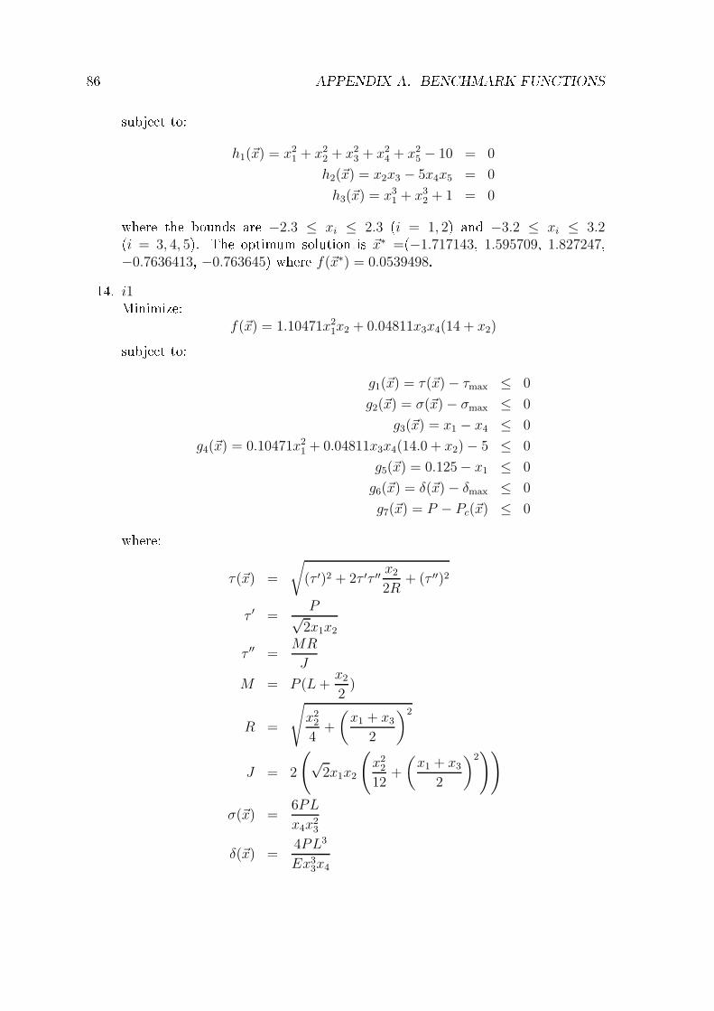
86 APPENDIX A. BENCHMARK FUNCTIONSsubje t to:h1(~x) = x2

1 + x22 + x2

3 + x24 + x2

5 − 10 = 0

h2(~x) = x2x3 − 5x4x5 = 0

h3(~x) = x31 + x3

2 + 1 = 0where the bounds are −2.3 ≤ xi ≤ 2.3 (i = 1, 2) and −3.2 ≤ xi ≤ 3.2(i = 3, 4, 5). The optimum solution is ~x∗ =(−1.717143, 1.595709, 1.827247,−0.7636413, −0.763645) where f(~x∗) = 0.0539498.14. i1Minimize:

f(~x) = 1.10471x21x2 + 0.04811x3x4(14 + x2)subje t to:

g1(~x) = τ(~x) − τmax ≤ 0

g2(~x) = σ(~x) − σmax ≤ 0

g3(~x) = x1 − x4 ≤ 0

g4(~x) = 0.10471x21 + 0.04811x3x4(14.0 + x2) − 5 ≤ 0

g5(~x) = 0.125 − x1 ≤ 0

g6(~x) = δ(~x) − δmax ≤ 0

g7(~x) = P − Pc(~x) ≤ 0where:τ(~x) =

√

(τ ′)2 + 2τ ′τ ′′x2

2R+ (τ ′′)2

τ ′ =P√

2x1x2

τ ′′ =MR

J

M = P (L+x2

2)

R =

√

x22

4+

(

x1 + x3

2

)2

J = 2

(

√2x1x2

(

x22

12+

(

x1 + x3

2

)2))

σ(~x) =6PL

x4x23

δ(~x) =4PL3

Ex33x4

87Pc(~x) =

4.013E

√

x2

3x6

4

36

L2

(

1 − x3

2L

√

E

4G

)and P = 6000lp, L = 14in, E = 30 × 106psi, g = 12 × 106psi, τmax = 13600psi,σmax = 30000psi, δmax = 0.25in. The bounds are 0.1 ≤ x1 ≤ 2, 0.1 ≤ x2 ≤ 10,0.1 ≤ x3 ≤ 10 and 0.1 ≤ x4 ≤ 2. The best known solution is ~x∗ =(0.2057296,3.4704887, 9.0366239, 0.205729) where f(~x∗) = 1.724852309.15. i2Minimize:

f(~x) = (0.6224)0.0625 ⌊x1⌋ x3x4 + (1.7781)0.0625 ⌊x2⌋ x23

+3.1661(0.0625 ⌊x1⌋)2x4 + 19.84(0.0625 ⌊x1⌋)2x3subje t to:g1(~x) = −0.0625 ⌊x1⌋ + 0.0193x3 ≤ 0

g2(~x) = −0.0625 ⌊x2⌋ + 0.00954x3 ≤ 0

g3(~x) = −πx23x4 −

4

3πx3

3 + 1296000 ≤ 0

g4(~x) = x4 − 240 ≤ 0where the bounds are 1 ≤ xi ≤ 99 (i = 1, 2) and 10 ≤ xi ≤ 200 (i = 3, 4).The best known solution is ~x∗ =(0.8125, 0.4375, 42.098445, 176.636597) wheref(~x∗) = 6059.71434795.16. i3Minimize:

f(~x) = (x3 + 2)x2x21subje t to:

g1(~x) = 1 − x32x3

71785x41

≤ 0

g2(~x) =4x2

2 − x1x2

12566(x2x31 − x4

1)+

1

5108x21

− 1 ≤ 0

g3(~x) = 1 − 140.45x1

x22x3

≤ 0

g4(~x) =x2 + x1

1.5− 1 ≤ 0where the bounds are 0.05 ≤ x1 ≤ 2, 0.25 ≤ x2 ≤ 1.3 and 2 ≤ x3 ≤ 15. Thebest known solution is ~x∗ =(0.051683, 0.0356577, 11.297236) where f(~x∗) =

0.012665.

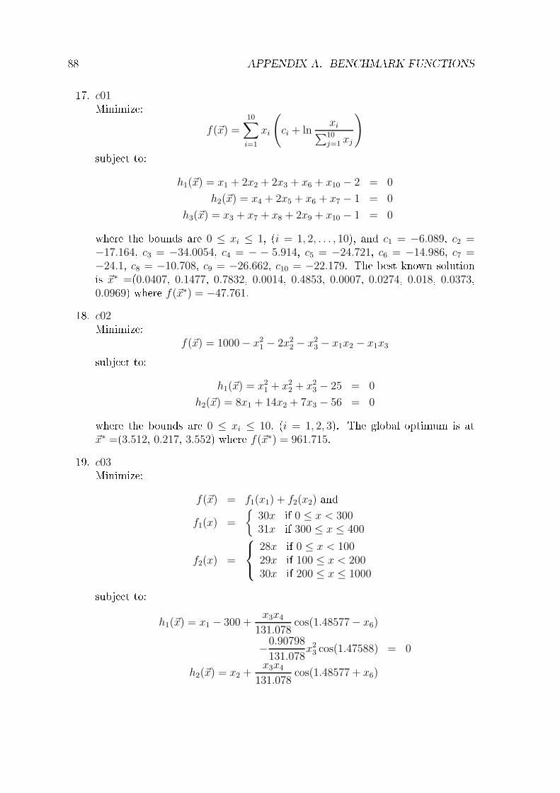
88 APPENDIX A. BENCHMARK FUNCTIONS17. c01Minimize:f(~x) =

10∑

i=1

xi

(

ci + lnxi

∑10j=1 xj

)subje t to:h1(~x) = x1 + 2x2 + 2x3 + x6 + x10 − 2 = 0

h2(~x) = x4 + 2x5 + x6 + x7 − 1 = 0

h3(~x) = x3 + x7 + x8 + 2x9 + x10 − 1 = 0where the bounds are 0 ≤ xi ≤ 1, (i = 1, 2, . . . , 10), and c1 = −6.089, c2 =−17.164, c3 = −34.0054, c4 = − − 5.914, c5 = −24.721, c6 = −14.986, c7 =−24.1, c8 = −10.708, c9 = −26.662, c10 = −22.179. The best known solutionis ~x∗ =(0.0407, 0.1477, 0.7832, 0.0014, 0.4853, 0.0007, 0.0274, 0.018, 0.0373,0.0969) where f(~x∗) = −47.761.18. c02Minimize:

f(~x) = 1000 − x21 − 2x2

2 − x23 − x1x2 − x1x3subje t to:

h1(~x) = x21 + x2

2 + x23 − 25 = 0

h2(~x) = 8x1 + 14x2 + 7x3 − 56 = 0where the bounds are 0 ≤ xi ≤ 10, (i = 1, 2, 3). The global optimum is at~x∗ =(3.512, 0.217, 3.552) where f(~x∗) = 961.715.19. c03Minimize:

f(~x) = f1(x1) + f2(x2) andf1(x) =

30x if 0 ≤ x < 30031x if 300 ≤ x ≤ 400

f2(x) =

28x if 0 ≤ x < 10029x if 100 ≤ x < 20030x if 200 ≤ x ≤ 1000subje t to:

h1(~x) = x1 − 300 +x3x4

131.078cos(1.48577− x6)

−0.90798

131.078x2

3 cos(1.47588) = 0

h2(~x) = x2 +x3x4

131.078cos(1.48577 + x6)

89−0.90798

131.078x2

4 cos(1.47588) = 0

h3(~x) = x5 +x3x4

131.078sin(1.48577 + x6)

−0.90798

131.078x2

4 sin(1.47588) = 0

h4(~x) = 200 − x3x4

131.078sin(1.48577− x6)

−0.90798

131.078x2

3 sin(1.47588) = 0where the bounds are 0 ≤ x1 ≤ 400, 0 ≤ x2 ≤ 1000, 340 ≤ x3 ≤ 420, 340 ≤x4 ≤ 420, −1000 ≤ x5 ≤ 1000, 0 ≤ x3 ≤ 0.5236. The best known solution is~x∗ =(107.81, 196.32, 373.83, 420, 21.31, 0.153) where f(~x∗) = 8927.5888.20. c04Maximize:

f(~x) = 0.5(x1x4 − x2x3 + x3x9 − x5x9 + x5x8 − x6x7)subje t to:g1(~x) = x2

3 + x24 − 1 ≤ 0

g2(~x) = x29 − 1 ≤ 0

g3(~x) = x25 + x2

6 − 1 ≤ 0

g4(~x) = x21 + (x2 − x9)

2 − 1 ≤ 0

g5(~x) = (x1 − x5)2 + (x2 − x6)

2 − 1 ≤ 0

g6(~x) = (x1 − x7)2 + (x2 − x8)

2 − 1 ≤ 0

g7(~x) = (x3 − x5)2 + (x4 − x6)

2 − 1 ≤ 0

g8(~x) = (x3 − x7)2 + (x4 − x8)

2 − 1 ≤ 0

g9(~x) = x27 + (x8 − x9)

2 − 1 ≤ 0

g10(~x) = x2x3 − x1x4 ≤ 0

g11(~x) = −x3x9 ≤ 0

g12(~x) = x5x9 ≤ 0

g13(~x) = x6x7 − x5x8 ≤ 0where the bounds are −1 ≤ xi ≤ 1 (i = 1, 2, . . . , 8). The best known solu-tion is ~x∗ =(0.9971, −0.0758, 0.553, 0.8331, 0.9981, −0.0623, 0.5642, 0.8256,0.0000024) where f(~x∗) = 0.866.21. c05Maximize:

f(~x) =

10∑

i=1

bixi −5∑

i=1

5∑

j=1

ci,jx10+ix10+j − 2

5∑

j=1

djx310+j

90 APPENDIX A. BENCHMARK FUNCTIONSsubje t to:gj(~x) =

10∑

i=1

ai,jxi − 2

5∑

i=1

ci,jx10+i − 3djx210+j − ej ≤ 0and

e = (−15,−27,−36,−18,−12)

c1 = (30,−20,−10, 32,−10)

c2 = (−20, 39,−6, 39,−20)

c3 = (−10,−6, 10,−6,−10)

c4 = (32,−31,−6, 39,−20)

c5 = (−10, 32,−10,−20, 30)

d = (4, 8, 10, 6, 2)

a1 = (−16, 2, 0, 1, 0)

a2 = (0,−2, 0, 4, 2)

a3 = (−35, 0, 2, 0, 0)

a4 = (0,−2, 0,−4,−1)

a5 = (0,−9,−2, 1,−2.8)

a6 = (2, 0,−4, 0, 0)

a7 = (−1,−1,−1,−1,−1)

a8 = (−1,−2,−3,−2,−1)

a9 = (1, 2, 3, 4, 5)

a10 = (1, 1, 1, 1, 1)where the bounds are 0 ≤ xi ≤ 100 (i = 1, 2, . . . , 15). The best known solutionis ~x∗ =(0, 0, 5.147, 0, 3.0611, 11.8395, 0, 0, 0.1039, 0, 0.3, 0.3335, 0.4, 0.4283,0.224) where f(~x∗) = −32.386.22. c06Minimize:

f(~x) = x1subje t to:g1(~x) = −x1 + 35x0.6

2 + 35x0.63 ≤ 0

h2(~x) = −300x3 + 7500x5 − 7500x6 − 25x4x5 + 25x4x6 + x3x4 = 0

h3(~x) = 100x2 + 155.365x4 + 2500x7 − x2x4 − 25x4x7 − 15536.5 = 0

h4(~x) = −x5 + ln(−x4 + 900) = 0

h5(~x) = −x6 + ln(x4 + 300) = 0

h6(~x) = −x7 + ln(−2x4 + 700) = 0

91where the bounds are 0 ≤ x1 ≤ 1000, 0 ≤ x2 ≤ 40, 0 ≤ x3 ≤ 40, 100 ≤ x4 ≤300, 6.3 ≤ x5 ≤ 6.7, 5.9 ≤ x6 ≤ 6.4, and 4.5 ≤ x7 ≤ 6.25. The best knownsolution is ~x∗ =(193.77835, 0, 17.3272, 100.01566, 6.6846, 5.9915, 6.2145) wheref(~x∗) = 193.7783.23. c07Minimize:

f(~x) = −9x5 − 15x8 + 6x1 + 16x2 + 10(x6 + x7)subje t to:h1(~x) = x1 + x2 − x3 − x4 = 0

h2(~x) = 0.03x1 + 0.01x2 − x9(x3 + x4) = 0

h3(~x) = x3 + x6 − x5 = 0

h4(~x) = x4 + x7 − x8 = 0

g5(~x) = x9x3 + 0.02x6 − 0.025x5 ≤ 0

g6(~x) = x9x4 + 0.02x7 − 0.025x8 ≤ 0where the bounds are 0 ≤ xi ≤ 300 (i = 1, 2, 6), 0 ≤ xi ≤ 100 (i = 3, 5, 7),0 ≤ xi ≤ 200 (i = 4, 8), and 0.01 ≤ x9 ≤ 0.03. The optimum solution is at~x∗ =(0, 100, 0, 100, 0, 0, 100, 200, 0.1) where f(~x∗) = −400.24. c08Minimize:

f(~x) = −x1 − x2subje t to:g1(~x) = −2x4

1 + 8x31 − 8x2

1 + x2 − 2 ≤ 0

g2(~x) = −4x41 + 32x3

1 − 88x21 + 96x1 + x2 − 36 ≤ 0where the bounds are 0 ≤ x1 ≤ 3 and 0 ≤ x2 ≤ 4. The optimum solution is at

~x∗ =(2.3295, 3.17846) where f(~x∗) = −5.5079.

92 APPENDIX A. BENCHMARK FUNCTIONS

Appendix BResults for the Mezura-CoelloBen hmarkThe results for the engineering problems proposed as ben hmark by Mezura andCoello [5 are in Tables B.2B.9. The optimal values for these problems are summa-rized in Table B.1. Fun tion Optimal value max/minc01 −47.761 Minimizec02 961.715 Minimizec03 8927.5888 Minimizec04 0.866 Maximizec05 −32.386 Maximizec06 193.7783493 Minimizec07 −400 Minimizec08 5.5079 MinimizeTable B.1: The known or reported optimum values for the rest of the test fun tions.The olumn max/min tells whether the problem is a maximization or a minimizationto better interpret the results.

93

94 APPENDIX B. RESULTS FOR THE MEZURA-COELLO BENCHMARKStatisti value ES(µ+ λ) B-ES(µ+ λ) DE_1 B-DE_1best -45.14793 -47.761 47.761 47.761worst -40.4601 -42.47365 47.759 47.6708mean -43.4492 -46.81045 47.7609 47.757median -43.449 -46.81045 47.761 47.761varian e 0.947 1.6654 1.021E-7 2.602E-4standard dev. 0.973 1.2654 3.196E-4 0.016# feasibles 0 0 0 0# ǫ-feasibles 30 30 30 30Table B.2: Results for fun tion c01. The se ond and third olumn represent the om-parison between the normal ES and the Baldwinian one, respe tively. The fourth andfth is the omparison between the normal DE and the Baldwinian one respe tively.Statisti value ES(µ+ λ) B-ES(µ+ λ) DE_1 B-DE_1best 961.7181 961.7244 961.7151 961.7151worst 969.401 966.21389 961.7151 961.7151mean 964.003 963.11675 961.7151 961.7151median 963.3009 962.8708 961.7151 961.7151varian e 4.689 1.74 3.761E-14 2.457E-12standard dev. 2.1654 1.319 1.939E-7 1.567E-6# feasibles 0 0 0 0# ǫ-feasibles 30 30 30 30Table B.3: Results for fun tion c02. The se ond and third olumn represent the om-parison between the normal ES and the Baldwinian one, respe tively. The fourth andfth is the omparison between the normal DE and the Baldwinian one respe tively.Statisti value ES(µ+ λ) B-ES(µ+ λ) DE_1 B-DE_1bestworstmeanmedianvarian estandard dev.# feasibles 0 0 0 0# ǫ-feasibles 30 30 30 30Table B.4: Results for fun tion c03. The se ond and third olumn represent the om-parison between the normal ES and the Baldwinian one, respe tively. The fourth andfth is the omparison between the normal DE and the Baldwinian one respe tively.

95Statisti value ES(µ+ λ) B-ES(µ+ λ) DE_1 B-DE_1best 0.866 0.866 0.866 0.866worst 0.512 0.571 0.866 0.866mean 0.7657 0.828 0.866 0.866median 0.8623 0.864 0.866 0.866varian e 0.0167 0.0081 5.05E-13 5.739E-11standard dev. 0.1294 0.0904 7.106E-7 7.575E-6# feasibles 30 30 30 30# ǫ-feasibles 30 30 30 30Table B.5: Results for fun tion c04. The se ond and third olumn represent the om-parison between the normal ES and the Baldwinian one, respe tively. The fourth andfth is the omparison between the normal DE and the Baldwinian one respe tively.Statisti value ES(µ+ λ) B-ES(µ+ λ) DE_1 B-DE_1bestworstmeanmedianvarian estandard dev.# feasibles 30 30 30 30# ǫ-feasibles 30 30 30 30Table B.6: Results for fun tion c05. The se ond and third olumn represent the om-parison between the normal ES and the Baldwinian one, respe tively. The fourth andfth is the omparison between the normal DE and the Baldwinian one respe tively.Statisti value ES(µ+ λ) B-ES(µ+ λ) DE_1 B-DE_1best 452.557 440.694 193.786 193.785worst 691.273 657.992 325.149 325.157mean 550.058 544.574 220.059 206.923median 539.914 536.7099 193.786 193.786varian e 3482.56 3481.63 2760.89 1553.06standard dev. 59.013 59.005 52.544 39.408# feasibles 0 0 0 0# ǫ-feasibles 30 30 30 30Table B.7: Results for fun tion c06. The se ond and third olumn represent the om-parison between the normal ES and the Baldwinian one, respe tively. The fourth andfth is the omparison between the normal DE and the Baldwinian one respe tively.

96 APPENDIX B. RESULTS FOR THE MEZURA-COELLO BENCHMARKStatisti value ES(µ+ λ) B-ES(µ+ λ) DE_1 B-DE_1best -401.92 -402.426 400 400worst -397.906 -397.756 399.943 399.789mean -400.21 -399.955 399.995 399.962median -400.335 -400.28 399.999 399.999varian e 1.0639 1.1892 1.17E-4 0.0036standard dev. 1.0314 1.0905 0.0108 0.0602# feasibles 0 0 0 0# ǫ-feasibles 30 30 30 30Table B.8: Results for fun tion c07. The se ond and third olumn represent the om-parison between the normal ES and the Baldwinian one, respe tively. The fourth andfth is the omparison between the normal DE and the Baldwinian one respe tively.

Statisti value ES(µ+ λ) B-ES(µ+ λ) DE_1 B-DE_1best 5.50801 5.50801 5.50801 5.50801worst 5.50801 5.50801 5.50801 5.50801mean 5.50801 5.50801 5.50801 5.50801median 5.50801 5.50801 5.50801 5.50801varian e 1.908E-16 7.045E-13 3.155E-30 3.155E-30standard dev. 1.381E-8 8.393E-7 1.776E-15 1.776E-15# feasibles 30 30 30 30# ǫ-feasibles 30 30 30 30Table B.9: Results for fun tion c08. The se ond and third olumn represent the om-parison between the normal ES and the Baldwinian one, respe tively. The fourth andfth is the omparison between the normal DE and the Baldwinian one respe tively.