-- BUSINESS PROPRIETARY -- © 2007 viaSim 1 Archived File The file below has been archived for historical reference purposes only. The content and links are no longer maintained and may be outdated. See the OER Public Archive Home Page for more details about archived files.

-- BUSINESS PROPRIETARY --© 2007 viaSim 1 Archived File The file below has been archived for historical reference purposes only. The content and links.
Dec 30, 2015
Welcome message from author
This document is posted to help you gain knowledge. Please leave a comment to let me know what you think about it! Share it to your friends and learn new things together.
Transcript

-- BUSINESS PROPRIETARY --© 2007 viaSim
1
Archived File
The file below has been archived for historical reference purposes only. The content and links are no
longer maintained and may be outdated. See the OER Public Archive Home Page for more details about
archived files.

A New Model for Predicting the Number of NIH Grant Applications
viaSim
J. Chris White
April 19, 2007
-- BUSINESS PROPRIETARY --© 2007 viaSim
3
Overview
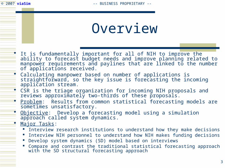
It is fundamentally important for all of NIH to improve the ability to forecast budget needs and improve planning related to manpower requirements and paylines that are linked to the number of applications received.
Calculating manpower based on number of applications is straightforward, so the key issue is forecasting the incoming application stream.
CSR is the triage organization for incoming NIH proposals and reviews approximately two-thirds of these proposals.
Problem: Results from common statistical forecasting models are sometimes unsatisfactory.
Objective: Develop a forecasting model using a simulation approach called system dynamics.
Major Tasks: Interview research institutions to understand how they make decisions Interview NIH personnel to understand how NIH makes funding decisions Develop system dynamics (SD) model based on interviews Compare and contrast the traditional statistical forecasting approach with the SD
structural forecasting approach
-- BUSINESS PROPRIETARY --© 2007 viaSim
4
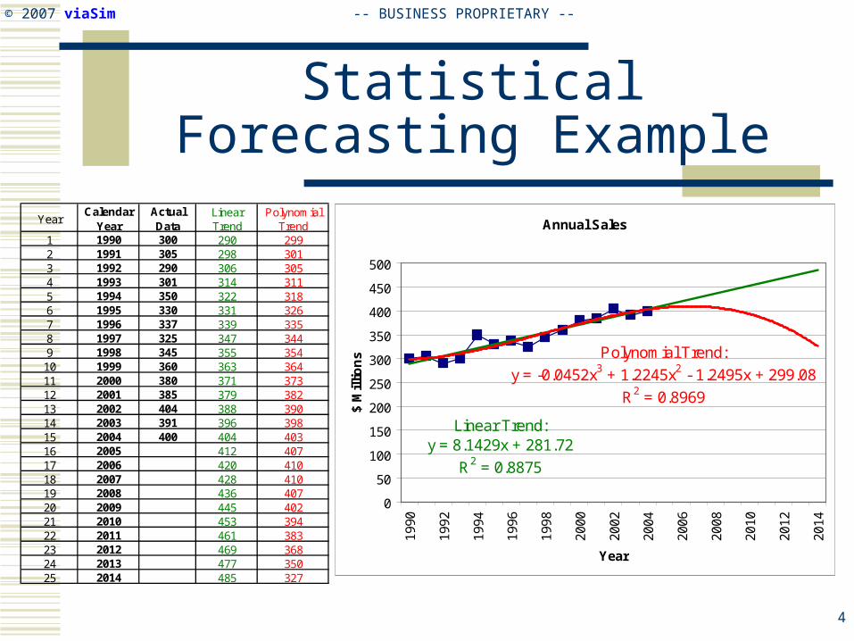
Statistical Forecasting Example
YearCalendar
YearActual Data
Linear Trend
Polynomial Trend
1 1990 300 290 2992 1991 305 298 3013 1992 290 306 3054 1993 301 314 3115 1994 350 322 3186 1995 330 331 3267 1996 337 339 3358 1997 325 347 3449 1998 345 355 35410 1999 360 363 36411 2000 380 371 37312 2001 385 379 38213 2002 404 388 39014 2003 391 396 39815 2004 400 404 40316 2005 412 40717 2006 420 41018 2007 428 41019 2008 436 40720 2009 445 40221 2010 453 39422 2011 461 38323 2012 469 36824 2013 477 35025 2014 485 327
0
50
100
150
200
250
300
350
400
450
500
1990
1992
1994
1996
1998
2000
2002
2004
2006
2008
2010
2012
2014
Year
1 1990 300 290 2992 1991 305 298 3013 1992 290 306 3054 1993 301 314 3115 1994 350 322 3186 1995 330 331 3267 1996 337 339 3358 1997 325 347 3449 1998 345 355 35410 1999 360 363 36411 2000 380 371 37312 2001 385 379 38213 2002 404 388 39014 2003 391 396 39815 2004 400 404 40316 2005 412 40717 2006 420 41018 2007 428 41019 2008 436 40720 2009 445 40221 2010 453 39422 2011 461 38323 2012 469 36824 2013 477 35025 2014 485 327
Annual Sales
Linear Trend:y = 8.1429x + 281.72
R2 = 0.8875
Polynomial Trend:
y = -0.0452x3 + 1.2245x2 - 1.2495x + 299.08
R2 = 0.8969
0
50
100
150
200
250
300
350
400
450
500
1990
1992
1994
1996
1998
2000
2002
2004
2006
2008
2010
2012
2014
Year
$ M
illi
on
s
-- BUSINESS PROPRIETARY --© 2007 viaSim
5
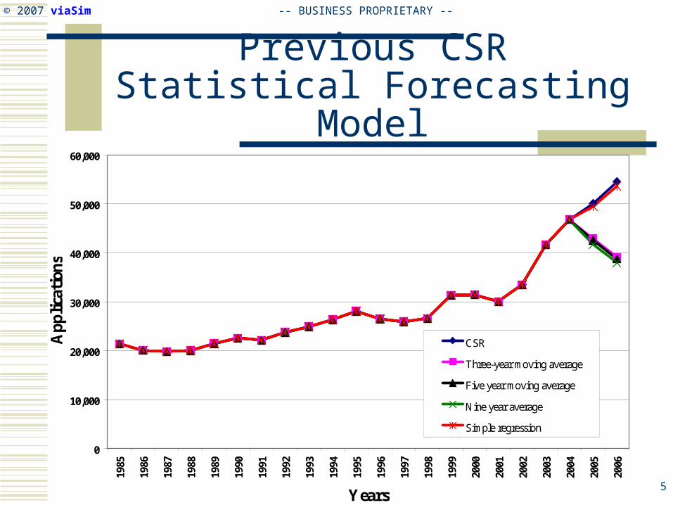
Previous CSR Statistical Forecasting Model
0
10,000
20,000
30,000
40,000
50,000
60,000
1985
1986
1987
1988
1989
1990
1991
1992
1993
1994
1995
1996
1997
1998
1999
2000
2001
2002
2003
2004
2005
2006
Years
Ap
pli
cati
ons
CSR
Three-year moving average
Five year moving average
Nine year average
Simple regression

-- BUSINESS PROPRIETARY --© 2007 viaSim
6
Meyers’ Statistical Forecast
Applications Based on Current (or Requested) Appropriations and Appropriations Levels Lagged One and Two Years
0
10,000
20,000
30,000
40,000
50,000
60,000
70,000
80,000
90,000
1998 1999 2000 2001 2002 2003 2004 2005 2006 2007 2008
Applications(t) Forecast
-- BUSINESS PROPRIETARY --© 2007 viaSim
7
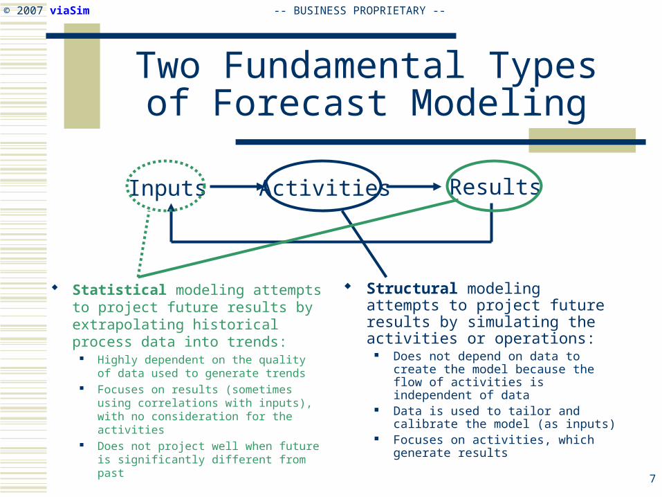
Two Fundamental Types of Forecast Modeling
Statistical modeling attempts to project future results by extrapolating historical process data into trends:
Highly dependent on the quality of data used to generate trends
Focuses on results (sometimes using correlations with inputs), with no consideration for the activities
Does not project well when future is significantly different from past
Structural modeling attempts to project future results by simulating the activities or operations:
Does not depend on data to create the model because the flow of activities is independent of data
Data is used to tailor and calibrate the model (as inputs)
Focuses on activities, which generate results
Activities ResultsInputs

-- BUSINESS PROPRIETARY --© 2007 viaSim
8
Model Scope
NIHBudget
AppsSubmitted
DesiredProportionNIH Funds
InstitutionStaff
+ + SuccessRate+_
+
CompletedGrants
+
NIHReviewCapacity
+ AppsReviewed+
AppsUnfunded
+++
RequiredFunds
+ FundingGap
+ –
_
_
+FundedGrants+
+
_ _
-- BUSINESS PROPRIETARY --© 2007 viaSim
9
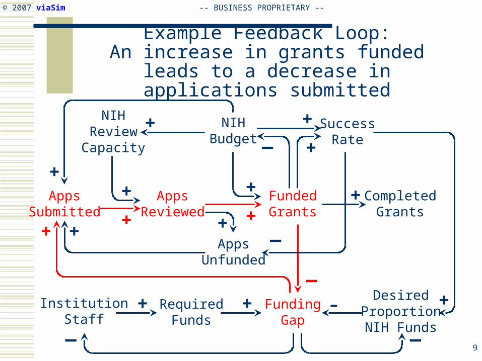
Example Feedback Loop:An increase in grants funded leads to a decrease in
applications submitted
NIHBudget
AppsSubmitted
DesiredProportionNIH Funds
InstitutionStaff
+ + SuccessRate+_
+
CompletedGrants
+
NIHReviewCapacity
+ AppsReviewed+
AppsUnfunded
+++
RequiredFunds
+ FundingGap
+ –
_
_
+FundedGrants+
+
_ _
-- BUSINESS PROPRIETARY --© 2007 viaSim
10
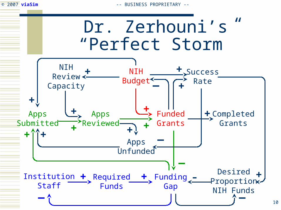
Dr. Zerhouni’s “Perfect Storm”
NIHBudget
AppsSubmitted
DesiredProportionNIH Funds
InstitutionStaff
+ + SuccessRate+_
+
CompletedGrants
+
NIHReviewCapacity
+ AppsReviewed+
AppsUnfunded
+++
RequiredFunds
+ FundingGap
+ –
_
_
+FundedGrants+
+
_ _
-- BUSINESS PROPRIETARY --© 2007 viaSim
11
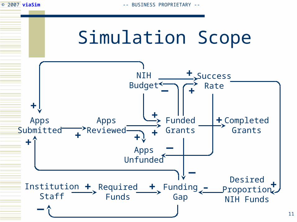
Simulation Scope
NIHBudget
AppsSubmitted
DesiredProportionNIH Funds
InstitutionStaff
+ SuccessRate+_
+
CompletedGrants
+AppsReviewed+
AppsUnfunded
++
RequiredFunds
+ FundingGap
+ –
_
_
+FundedGrants+
+
_
-- BUSINESS PROPRIETARY --© 2007 viaSim
12
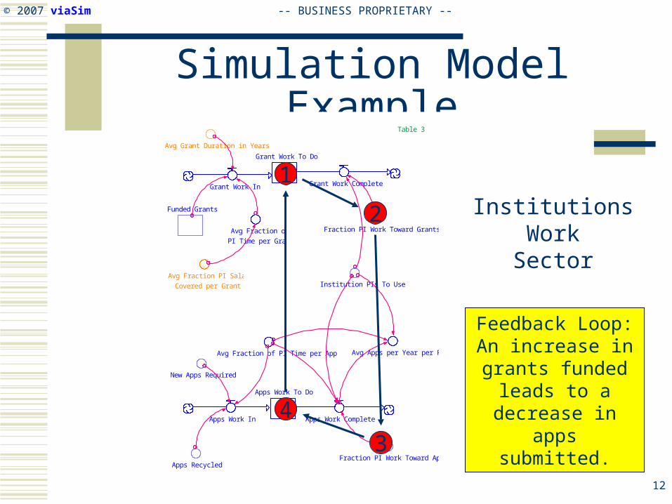
Simulation Model Example
InstitutionsWorkSector
Grants Completed at NIH
Apps in Review at NIH Grants Funded by NIH
Apps Accepted by NIH
Apps Rejected by NIH
Apps into NIH
Avg Success Rate
Avg $ per Grant Total
~
NIH Annual Budget
~
NIH Grant Funds Available
NIH Funds In NIH Funds Out
Obligation Ratio
Table 4
Avg Grant Duration in Years
Apps Recycled
Apps Not Recycled
Avg Fraction Not Recycled
New Apps Required
Apps Submitted
Avg Review Time
Avg Grant Duration in Years
Avg Salary per PI To Use
Obligated Funds
Acceptable App Review Delay
Avg $ per Grant per Year
Completed Grants
Max Apps Reviewed
Init Avg Success Rate to Use
Init Obligation Ratio to Use
Institution PIs To Use
Avg Grant Duration in Years
New Apps to Fund
Funds
~
Institution PIs To Use
Avg $ per Grant per Year
Apps in Review Funded GrantsApps Work Complete
Apps Submitted Apps Accepted Completed Grants
Apps to Recycle
Apps Rejected
Funded Grants
Avg Grant Duration in Years
Apps Accepted by NIH
Graph 1
Apps Rejected by NIH ~
Avg Fraction PI Salary
Covered per Grant
New Apps Required
Table 3Obligated Funds
~
~
Avg Salary per PI
Desired PI Funding per Year
Total Salaries
Actual PI Funding per Year
~
Grant Work To DoFunds
Funds In Funds Out
Avg Salary per PI To Use
PI Funding Gap
~
Avg $ per Grant per Year
~
Avg Success Rate
Avg Grant Duration in Years
NIH Staff To Use
Apps Accepted by NIH
Init Apps in Review at NIH
Init Avg Fraction Not Recycled
Apps Recycled
New Grants Required
Grant Work In Grant Work Complete
Funded Grants
Avg Fraction of
PI Time per Grant
Total Work To Do
Table 5
Avg Fraction of PI Time per App
Fraction PI Work Toward Grants
Avg Apps per Year per PI
Apps Work To Do
Apps Work In Apps Work Complete
Fraction PI Work Toward Apps
Grant Work To Do
Apps Work To Do
Fraction Grant Work
Fraction Apps Work
Avg Fraction of PI Time per App
Fraction PI Work Toward Grants
Fraction PI Work Toward Apps
Grant Work Complete
Total Salaries
Institution PIs To Use
NIH Staff To Use
Table 1
Avg Success Rate
Institution PIs To Use
Table 2
Institutions
NIH
Feedback Loop:An increase in grants
funded leads to a decrease in apps
submitted.
1
2
3
4

-- BUSINESS PROPRIETARY --© 2007 viaSim
13
Previous Simulation Results:Apps Reviewed by CSR
0
10000
20000
30000
40000
50000
60000
70000
80000
2000 2001 2002 2003 2004 2005 2006 2007 2008
Actual
Simulation

-- BUSINESS PROPRIETARY --© 2007 viaSim
14
New Baseline Simulation Results

Demonstration
-- BUSINESS PROPRIETARY --© 2007 viaSim
16
Next Steps
Train NIH staff in use of simulation tool. Finalize any reporting requirements. Model enhancements:
Expand to include more internal NIH processes and policies (e.g., review processes).
Expand to include more operational processes at institutions (e.g., facility expansions).
Integrate with PI simulation model.

Appendix
System Dynamics Methodology

-- BUSINESS PROPRIETARY --© 2007 viaSim
18
Why System Dynamics (SD)?
Ability toinfluenceresults
Organizational structure, IT systems,business processes, financial processes, etc.Structure
Corporate growth, inventory oscillations,labor force oscillations, etc.Behavior
Stock out, excess inventory, layoff, etc.Results
In any system, structure guides behavior,and behavior determines results.

-- BUSINESS PROPRIETARY --© 2007 viaSim
19
System Dynamics Methodology Personnel
Add Personnel Remove Personnel
Work To Do
Incoming Work Completed Work
Cash Balance
Revenue Expenses
2. Water accumulates
in tub
Good analogy: Water in bathtub
3. Water flows out
through drain
2. Money accumulates in “Cash Balance”
1. Water flows in through
faucet
3. Money flows out through “Expenses”
1. Money flows in through “Revenue”
-- BUSINESS PROPRIETARY --© 2007 viaSim
20
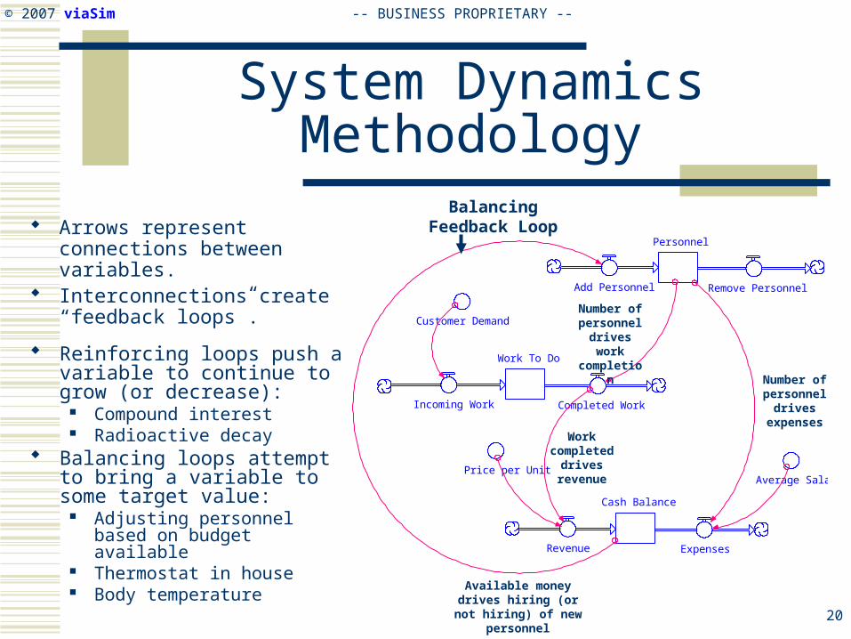
System Dynamics Methodology
Reinforcing loops push a variable to continue to grow (or decrease):
Compound interest Radioactive decay
Balancing loops attempt to bring a variable to some target value:
Adjusting personnel based on budget available
Thermostat in house Body temperature
Personnel
Add Personnel Remove Personnel
Work To Do
Incoming Work Completed Work
Cash Balance
Revenue Expenses
Average SalaryPrice per Unit
Customer Demand
Number of personnel
drives expenses
Number of personnel
drives work completion
Work completed
drives revenue
Available money drives hiring (or not hiring) of
new personnel
Balancing Feedback Loop Arrows represent connections
between variables. Interconnections create “feedback
loops”.

-- BUSINESS PROPRIETARY --© 2007 viaSim
21
What Makes SD Different?
SD creates an “operational”, working model of activities.
SD captures “feedback loops”, which are the function of management.
Ex: Cutting back when overbudget Ex: Adjusting the workforce to meet demand
SD captures time delays and non-linear relationships that can significantly impact performance.
Ex: Full impact of new policies not realized until several years later. Ex: Doubling of labor force does not always double throughput.
Related Documents
![NATIONAL AGRICULTURAL LIBRARY ARCHIVED FILE Archived …€¦ · minorbreeds.htm[1/15/2015 2:16:51 PM] Selected Readings on the History and Use of Old Livestock Breeds "Selection](https://static.cupdf.com/doc/110x72/5fbb28853947ea1e147ca378/national-agricultural-library-archived-file-archived-1152015-21651-pm-selected.jpg)


