© Boardworks Ltd 2006 1 of 57 These icons indicate that teacher’s notes or useful web addresses are available in the Not This icon indicates the slide contains activities created in Flash. These activities are not edita For more detailed instructions, see the Getting Started presentation. © Boardworks Ltd 2006 1 of 57 A2-Level Maths: Statistics 2 for Edexcel S2.4 Hypothesis tests

© Boardworks Ltd 20061 of 57 These icons indicate that teacher’s notes or useful web addresses are available in the Notes Page. This icon indicates the.
Dec 14, 2015
Welcome message from author
This document is posted to help you gain knowledge. Please leave a comment to let me know what you think about it! Share it to your friends and learn new things together.
Transcript

© Boardworks Ltd 20061 of 57
These icons indicate that teacher’s notes or useful web addresses are available in the Notes Page.
This icon indicates the slide contains activities created in Flash. These activities are not editable.
For more detailed instructions, see the Getting Started presentation.
© Boardworks Ltd 20061 of 57
A2-Level Maths: Statistics 2for Edexcel
S2.4 Hypothesis tests
© Boardworks Ltd 20062 of 57
Co
nte
nts
© Boardworks Ltd 20062 of 57
Introduction to sampling
Introduction to sampling
Introduction to hypothesis testing
Chocolate tasting practical
One-sided hypothesis tests
One-sided versus two-sided tests
Critical regions
Hypothesis tests and critical regions

© Boardworks Ltd 20063 of 57
The British government carries out a census of the entire population of the United Kingdom every 10 years (most recently in April 2001).
The first census in the United Kingdom was carried out in 1086 with the construction of the Doomesday Book. However they have only been conducted on a regular basis since 1801.
The census provides the government with a detailed picture of the population living in each part of the country (town, city or countryside). The results are used to help plan public services (health, housing, transport and education) for the future.
National census
© Boardworks Ltd 20064 of 57
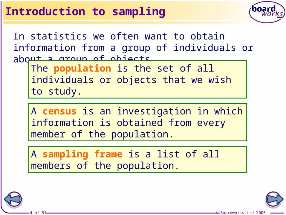
In statistics we often want to obtain information from a group of individuals or about a group of objects.
Introduction to sampling
A sampling frame is a list of all members of the population.
A census is an investigation in which information is obtained from every member of the population.
The population is the set of all individuals or objects that we wish to study.

© Boardworks Ltd 20065 of 57
Introduction to sampling
Examples:
1. A head teacher is interested in finding out how long her sixth form students spend in part-time employment each week.
The population is the set of all sixth form students in her school. A possible sampling frame would be the registers of sixth form tutor groups.
2. A newspaper is interested in obtaining the views of residents living close to the site of a proposed new airport.
The population might be all adults living within a 10 mile radius of the site. A possible sampling frame could be the local electoral roll.
© Boardworks Ltd 20066 of 57
Examples:
3. A car company has discovered a fault that affects one of their models of car. The company may wish to know how widespread the problem might be.
The population would be all cars produced of this particular model.
A possible sampling frame would be a list of all registered cars of this model provided by the DVLA.
Introduction to sampling
© Boardworks Ltd 20067 of 57
Carrying out a census of the entire population is usually not feasible or sensible.
Introduction to sampling
money
time
resources
In addition, some investigations could result in the destruction of the entire population!
For example, if a light bulb manufacturer wished to investigate the lifetime of its bulbs, a census would result in the destruction of all the bulbs it produced.
A census is usually costly in terms of
© Boardworks Ltd 20068 of 57
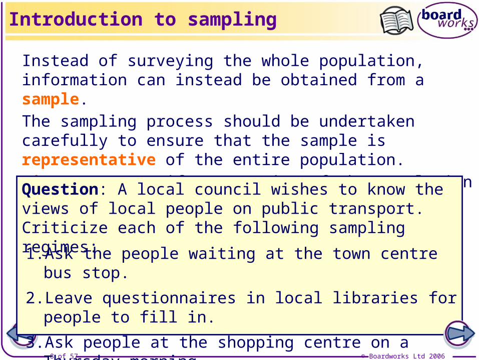
Instead of surveying the whole population, information can instead be obtained from a sample. The sampling process should be undertaken carefully to ensure that the sample is representative of the entire population. Bias can occur if one section of the population is over- or under-represented.
Introduction to sampling
Question: A local council wishes to know the views of local people on public transport. Criticize each of the following sampling regimes:
1. Ask the people waiting at the town centre bus stop.
2. Leave questionnaires in local libraries for people to fill in.
3. Ask people at the shopping centre on a Thursday morning.
© Boardworks Ltd 20069 of 57
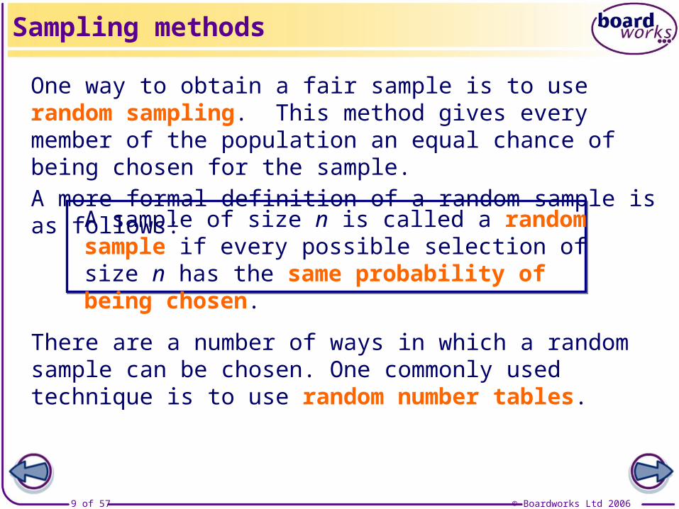
One way to obtain a fair sample is to use random sampling. This method gives every member of the population an equal chance of being chosen for the sample.A more formal definition of a random sample is as follows:
There are a number of ways in which a random sample can be chosen. One commonly used technique is to use random number tables.
Sampling methods
A sample of size n is called a random sample if every possible selection of size n has the same probability of being chosen.
© Boardworks Ltd 200610 of 57
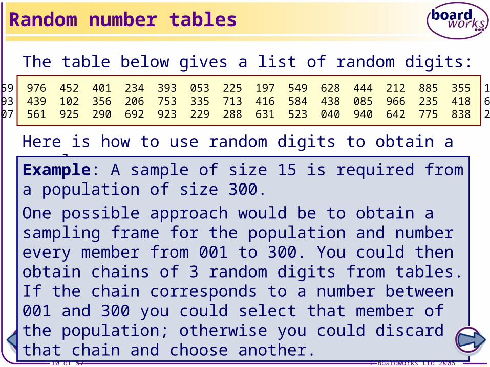
The table below gives a list of random digits:
793 259 976 452 401 234 393 053 225 197 549 628 444 212 885 355 169 905834 193 439 102 356 206 753 335 713 416 584 438 085 966 235 418 626 411469 807 561 925 290 692 923 229 288 631 523 040 940 642 775 838 281 475
Here is how to use random digits to obtain a sample:
Random number tables
Example: A sample of size 15 is required from a population of size 300.
One possible approach would be to obtain a sampling frame for the population and number every member from 001 to 300. You could then obtain chains of 3 random digits from tables. If the chain corresponds to a number between 001 and 300 you could select that member of the population; otherwise you could discard that chain and choose another.
© Boardworks Ltd 200611 of 57
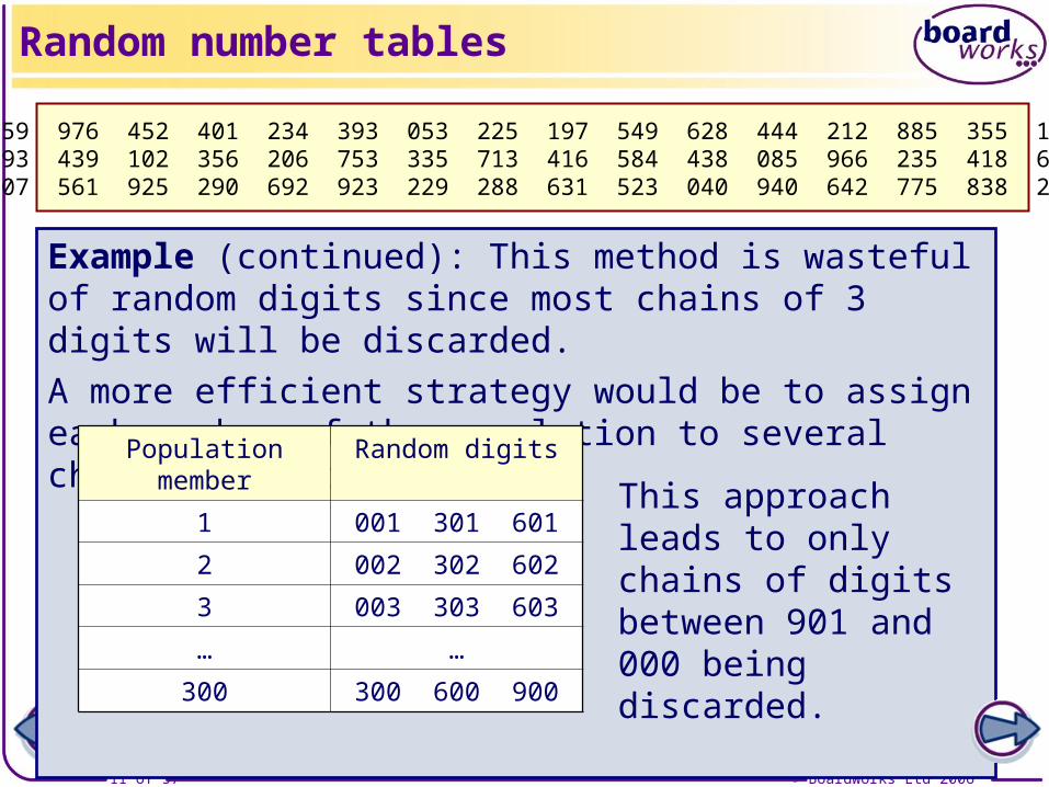
Example (continued): This method is wasteful of random digits since most chains of 3 digits will be discarded.
A more efficient strategy would be to assign each member of the population to several chains of random digits:
Random number tables
Population member Random digits
1 001 301 601
2 002 302 602
3 003 303 603
… …
300 300 600 900
This approach leads to only chains of digits between 901 and 000 being discarded.
793 259 976 452 401 234 393 053 225 197 549 628 444 212 885 355 169 905834 193 439 102 356 206 753 335 713 416 584 438 085 966 235 418 626 411469 807 561 925 290 692 923 229 288 631 523 040 940 642 775 838 281 475
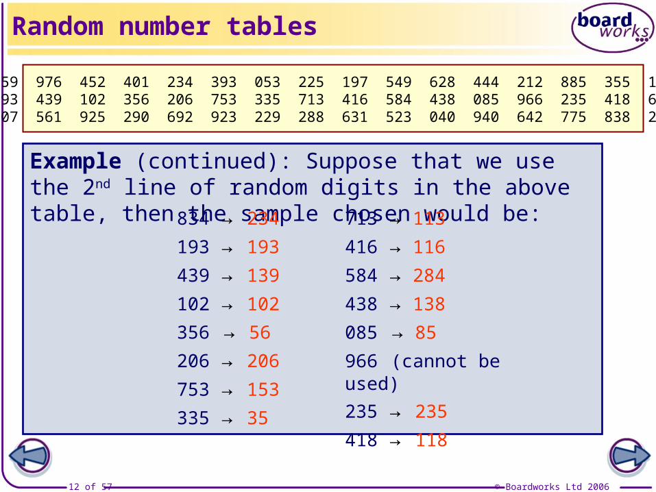
© Boardworks Ltd 200612 of 57
Example (continued): Suppose that we use the 2nd line of random digits in the above table, then the sample chosen would be: 834 → 234
193 → 193
439 → 139
102 → 102
356 → 56
206 → 206
753 → 153
335 → 35
713 → 113
416 → 116
584 → 284
438 → 138
085 → 85
966 (cannot be used)
235 → 235
418 → 118
Random number tables
793 259 976 452 401 234 393 053 225 197 549 628 444 212 885 355 169 905834 193 439 102 356 206 753 335 713 416 584 438 085 966 235 418 626 411469 807 561 925 290 692 923 229 288 631 523 040 940 642 775 838 281 475
© Boardworks Ltd 200613 of 57
Introduction to sampling
Introduction to hypothesis testing
Chocolate tasting practical
One-sided hypothesis tests
One-sided versus two-sided tests
Critical regions
Hypothesis tests and critical regions
Co
nte
nts
© Boardworks Ltd 200613 of 57
Hypothesis testing
© Boardworks Ltd 200614 of 57
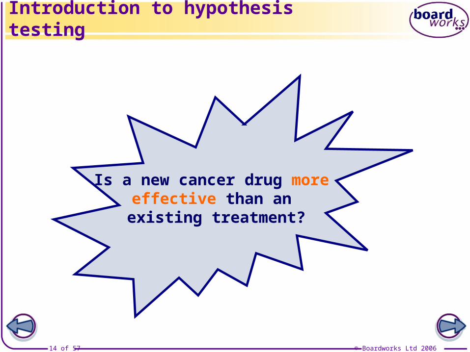
Is a new cancer drug more effective than an
existing treatment?
Introduction to hypothesis testing

© Boardworks Ltd 200615 of 57
Has the installation of a new speed camera led to a reduction in the
traffic speed?
Introduction to hypothesis testing

© Boardworks Ltd 200616 of 57
A candidate in an election claims 60%
support. Is the candidate exaggerating their level of support?
Introduction to hypothesis testing
© Boardworks Ltd 200617 of 57
Hypothesis testing is concerned with trying to answer questions like these.
Hypothesis tests are crucial in many subject areas including medicine, psychology, biology and geography.
In S1, we only deal with situations where we are testing a probability or a proportion.
Introduction to hypothesis testing

© Boardworks Ltd 200618 of 57
Consider the following simple situation.
You suspect that a die is biased towards the number six.
In order to test this suspicion, you could perform an experiment in which the die is thrown 20 times.
If the die were fair, you would expect about 3 sixes.
If you obtained a lot more than 3 sixes then you might decide that there is evidence to support your suspicions.
But how do you decide on what a suspicious number of sixes is?
A simple introductory example
© Boardworks Ltd 200619 of 57
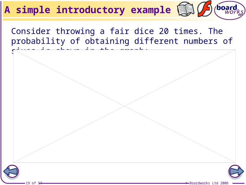
Consider throwing a fair dice 20 times. The probability of obtaining different numbers of sixes is shown in the graph:
A simple introductory example
© Boardworks Ltd 200620 of 57
So, we noticed from the previous slide that, with 20 throws of a fair die, the probability of getting 7 or more sixes is about 0.0371.
This means that if a fair die were thrown 20 times over and over again, then you would obtain 7 or more sixes less than once in every 20 experiments.
The figure of 1 in 20 (or 5%) is often taken as a cut-off point – results with probabilities below this level are sometimes regarded as being unlikely to have occurred by chance.
However, in situations where more evidence is required, cut-off values of 1% or 0.1% are typically used.
A simple introductory example

© Boardworks Ltd 200621 of 57
In hypothesis testing we are essentially presented with two rival hypotheses.
Examples might include:
A formal introduction to hypothesis tests
These rival hypotheses are referred to as the null and the alternative hypotheses.
“The coin is fair” or “the coin is biased”;
“The proportion of local people in favour of a by-pass is 80%” or “the proportion is smaller than 80%”;
“The drug has the same effectiveness as an existing treatment” or “the drug is more effective”.
© Boardworks Ltd 200622 of 57
The null hypothesis (H0) is often thought of as the cautious hypothesis – it represents the usual state of affairs.
The alternative hypothesis (H1) is usually the one that we suspect or hope to be true.
Hypothesis testing is concerned with examining the data collected in experiments, and deciding how likely the result is to have occurred if the null hypothesis is true.
The significance level of the test is the chosen cut-off value between the results that might plausibly have been obtained by chance if H0 is true, and the results that are unlikely to have occurred.
A formal introduction to hypothesis tests
© Boardworks Ltd 200623 of 57
Significance levels that are typically used are 10%, 5%, 1% and 0.1%.
These significance levels correspond to different rigours of test – the lower the significance level, the stronger the evidence the test will provide.
A formal introduction to hypothesis tests
Note: It is important to appreciate that it is not possible to prove that a hypothesis is definitely true in statistics. Hypothesis tests can only provide different degrees of
evidence in support of a hypothesis. A 10% significance level can only provide weak evidence in support of a hypothesis. A 0.1% test is much more
stringent and can provide very strong evidence.
© Boardworks Ltd 200624 of 57
Introduction to sampling
Introduction to hypothesis testing
Chocolate tasting practical
One-sided hypothesis tests
One-sided versus two-sided tests
Critical regions
Hypothesis tests and critical regions
Co
nte
nts
© Boardworks Ltd 200624 of 57
Chocolate tasting practical

© Boardworks Ltd 200625 of 57
Do you think you can taste the difference between branded chocolate and supermarket own-label chocolate?
You are going to perform an experiment to find out.
There will be 2 pieces of chocolate to try: one will be a branded make of chocolate, the other will be a supermarket’s own-brand. Try to identify the branded make.
Chocolate tasting practical

© Boardworks Ltd 200626 of 57
Chocolate tasting practical
© Boardworks Ltd 200627 of 57
Introduction to sampling
Introduction to hypothesis testing
Chocolate tasting practical
One-sided hypothesis tests
One-sided versus two-sided tests
Critical regions
Hypothesis tests and critical regions
Co
nte
nts
© Boardworks Ltd 200627 of 57
One-sided hypothesis tests

© Boardworks Ltd 200628 of 57
Example: Mr Jones, a candidate in a local election, claims to have the support of 40% of the electorate.
A rival candidate, Miss Smith, believes that Mr Jones is exaggerating his level of support.
She asks a random sample of 12 local people and discovers that 3 of them support Mr Jones.
Carry out a test at the 5% significance level to see whether there is evidence that Mr Jones is exaggerating his level of support.
One-sided hypothesis tests
© Boardworks Ltd 200629 of 57
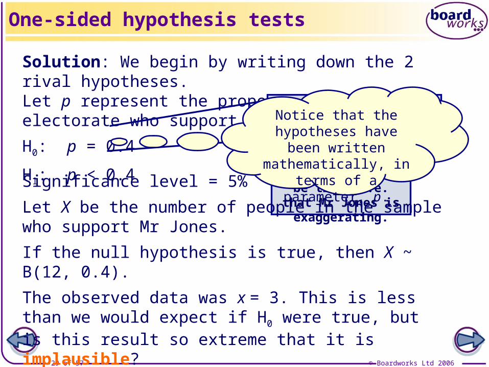
Solution: We begin by writing down the 2 rival hypotheses. Let p represent the proportion of the electorate who support Mr Jones.
H0: p = 0.4
H1: p < 0.4
This hypothesis represents our cautious belief, i.e. that Mr Jones is not lying about
his support.This hypothesis represents what is
suspected to be true, i.e. that Mr Jones is
exaggerating.
Notice that the hypotheses have been written mathematically, in terms of a parameter,
p.Significance level = 5%
Let X be the number of people in the sample who support Mr Jones.
If the null hypothesis is true, then X ~ B(12, 0.4).
The observed data was x = 3. This is less than we would expect if H0 were true, but is this result so extreme that it is implausible?
One-sided hypothesis tests
© Boardworks Ltd 200630 of 57
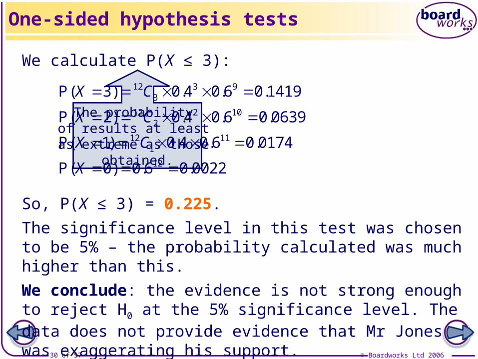
We calculate P(X ≤ 3):
The probability of results at least
as extreme as those obtained.
One-sided hypothesis tests
( ) . . .
( ) . . .
( ) . . .
( ) . .
12 3 93
12 2 102
12 111
12
P 3 0 4 0 6 0 1419
P 2 0 4 0 6 0 0639
P 1 0 4 0 6 0 0174
P 0 0 6 0 0022
X C
X C
X C
X
So, P(X ≤ 3) = 0.225.
The significance level in this test was chosen to be 5% – the probability calculated was much higher than this.
We conclude: the evidence is not strong enough to reject H0 at the 5% significance level. The data does not provide evidence that Mr Jones was exaggerating his support.
© Boardworks Ltd 200631 of 57
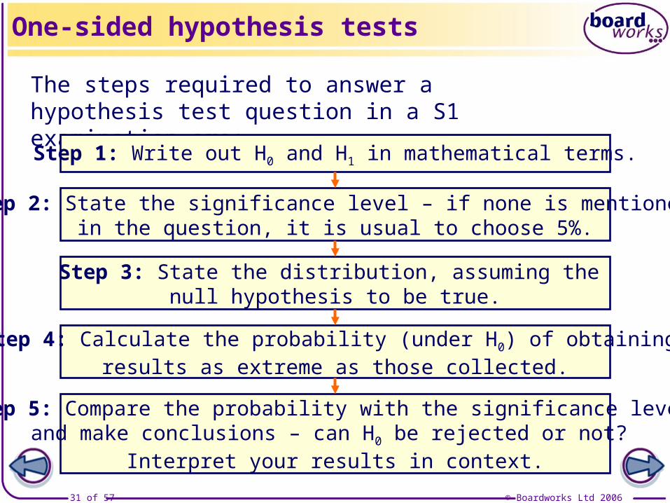
The steps required to answer a hypothesis test question in a S1 examination are:
Step 1: Write out H0 and H1 in mathematical terms.
Step 2: State the significance level – if none is mentioned in the question, it is usual to choose 5%.
Step 3: State the distribution, assuming the null hypothesis to be true.
Step 4: Calculate the probability (under H0) of obtaining results as extreme as those collected.
Step 5: Compare the probability with the significance level and make conclusions – can H0 be rejected or not?
Interpret your results in context.
One-sided hypothesis tests

© Boardworks Ltd 200632 of 57
Examination style question: The standard treatment for a particular medical condition has a success rate of 70%. A new drug is launched which, it is claimed, treats a greater proportion of patients successfully.
A doctor tries the new drug on 20 patients and finds that it successfully treats 19 of them.
Test at the 1% significance level whether there is evidence to suggest that the new drug treatment is more successful than the standard treatment.
One-sided hypothesis tests

© Boardworks Ltd 200633 of 57
Solution: Let p represent the proportion of patients that are treated successfully.
H0: p = 0.7
H1: p > 0.7
The new treatment is no more successful
than the existing treatment.
The new treatment is better than the
standard treatment.Significance level = 1%
Let X be the number of people successfully treated by the new drug.
If the null hypothesis is true, then X ~ B(20, 0.7).
The observed data is x = 19. Using tables, P(X ≥ 19) = 0.0076 < 1%.
We reject the null hypothesis at the 1% level – there is quite strong evidence that the new treatment is more successful.
One-sided hypothesis tests
© Boardworks Ltd 200634 of 57
Introduction to sampling
Introduction to hypothesis testing
Chocolate tasting practical
One-sided hypothesis tests
One-sided versus two-sided tests
Critical regions
Hypothesis tests and critical regions
Co
nte
nts
© Boardworks Ltd 200634 of 57
One-sided versus two-sided tests

© Boardworks Ltd 200635 of 57
The examples considered so far can all be classified as one-sided tests – we have been testing for either an increase or a decrease in the value of the parameter, p.
Sometimes we are not looking specifically for an increase (or decrease) in p, but instead we may want to examine whether the value of p has changed. In these situations we use a two-sided (or a two-tailed) test.
A two-sided hypothesis test carried out at the α% significance level is in a sense two separate one-sided tests. The significance level is therefore shared between these two tests, ½α% for each tail.
One-sided versus two-sided tests

© Boardworks Ltd 200636 of 57
Example: A restaurant has traditionally found that 60% of its customers have been pleased or very pleased with the quality of the food served.
A new chef is appointed and the restaurant management wish to find out whether this has changed the proportion of customers who are happy with their food.
The management question 16 diners and discover that 14 of them are pleased or very pleased with their food.
Test at the 5% significance level whether there has been a change in the proportion of contented customers.
One-sided versus two-sided tests
© Boardworks Ltd 200637 of 57
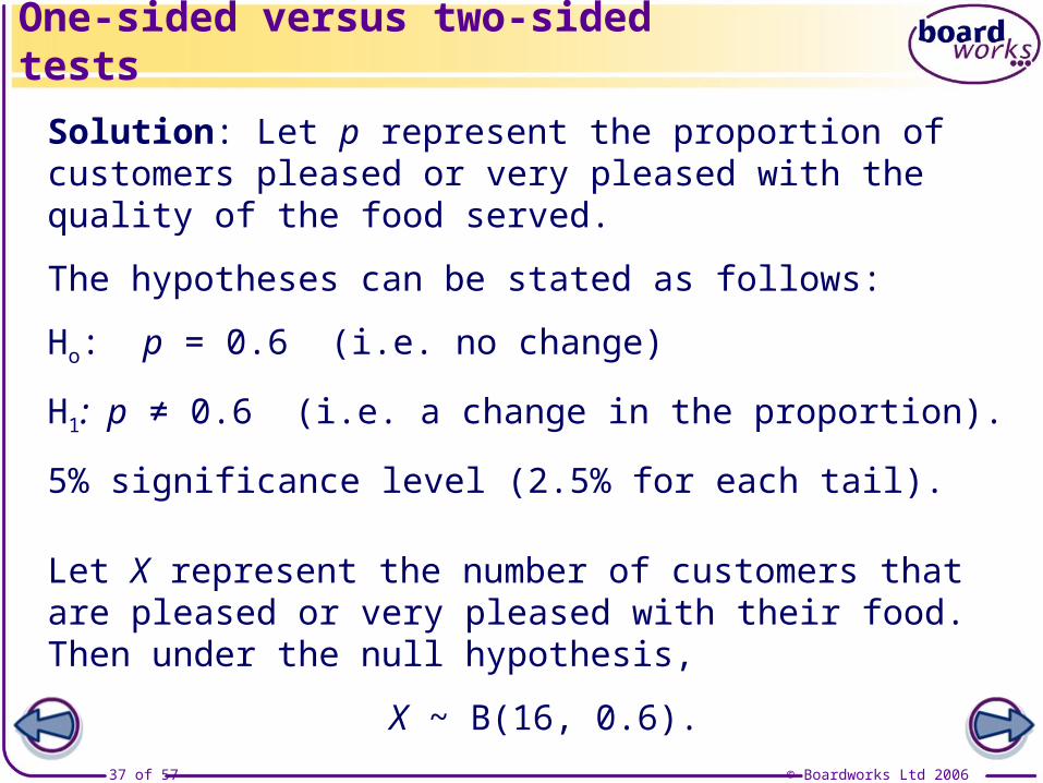
Solution: Let p represent the proportion of customers pleased or very pleased with the quality of the food served.
The hypotheses can be stated as follows:
Ho: p = 0.6 (i.e. no change)
H1: p ≠ 0.6 (i.e. a change in the proportion).
5% significance level (2.5% for each tail).
Let X represent the number of customers that are pleased or very pleased with their food. Then under the null hypothesis,
X ~ B(16, 0.6).
One-sided versus two-sided tests
© Boardworks Ltd 200638 of 57
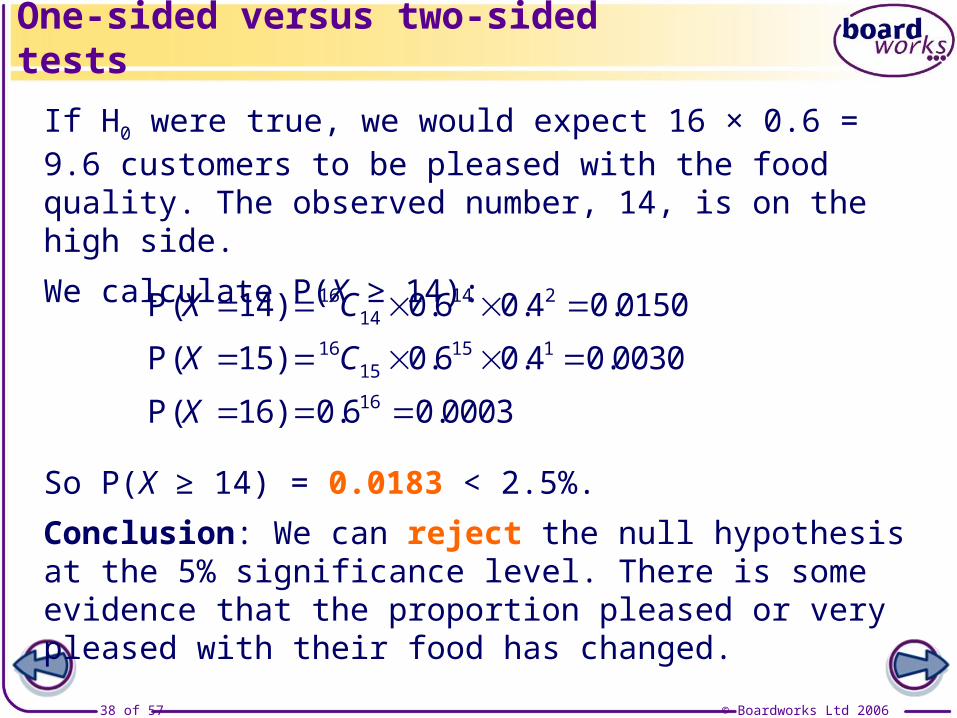
If H0 were true, we would expect 16 × 0.6 = 9.6 customers to be pleased with the food quality. The observed number, 14, is on the high side.
We calculate P(X ≥ 14):
One-sided versus two-sided tests
( ) . . .
( ) . . .
( ) . .
16 14 214
16 15 115
16
P 14 0 6 0 4 0 0150
P 15 0 6 0 4 0 0030
P 16 0 6 0 0003
X C
X C
X
So P(X ≥ 14) = 0.0183 < 2.5%.
Conclusion: We can reject the null hypothesis at the 5% significance level. There is some evidence that the proportion pleased or very pleased with their food has changed.
© Boardworks Ltd 200639 of 57
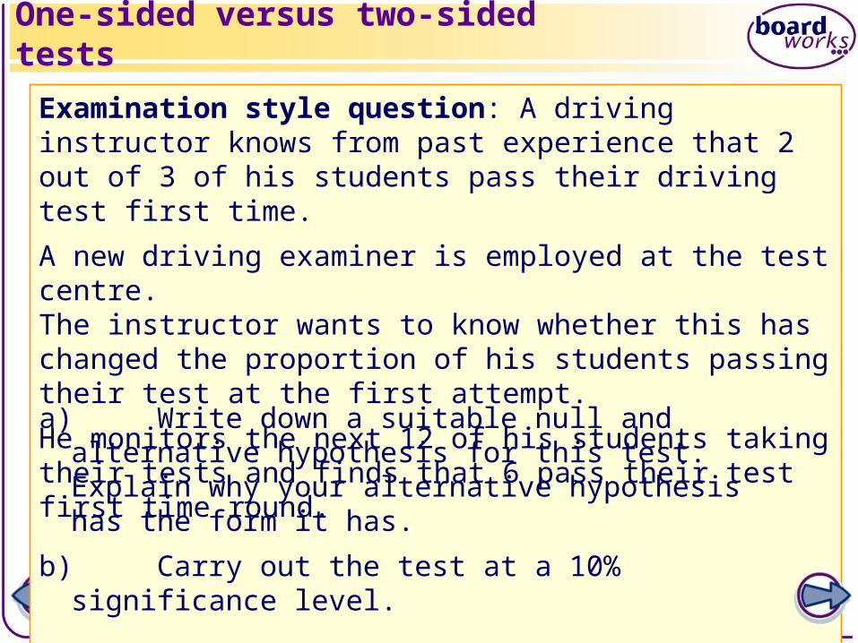
Examination style question: A driving instructor knows from past experience that 2 out of 3 of his students pass their driving test first time.
A new driving examiner is employed at the test centre. The instructor wants to know whether this has changed the proportion of his students passing their test at the first attempt.
He monitors the next 12 of his students taking their tests and finds that 6 pass their test first time round.
One-sided versus two-sided tests
a) Write down a suitable null and alternative hypothesis for this test. Explain why your alternative hypothesis has the form it has.
b) Carry out the test at a 10% significance level.
© Boardworks Ltd 200640 of 57
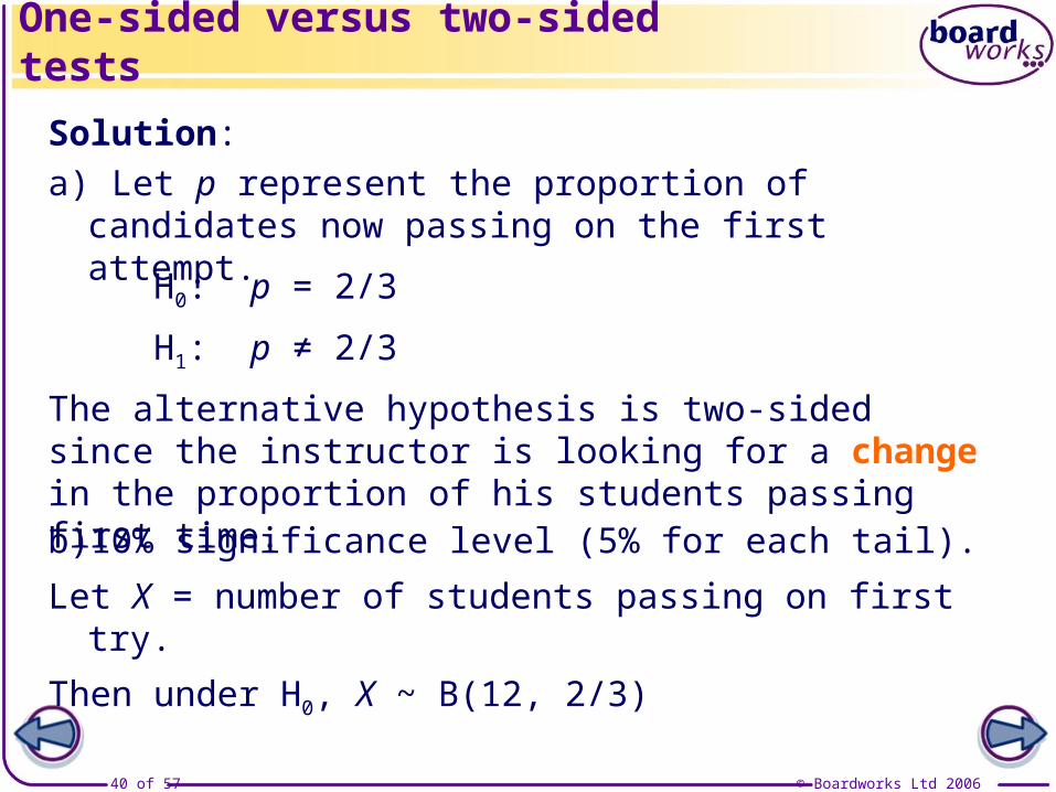
Solution:
H0: p = 2/3
H1: p ≠ 2/3
The alternative hypothesis is two-sided since the instructor is looking for a change in the proportion of his students passing first time.
One-sided versus two-sided tests
b) 10% significance level (5% for each tail).
Let X = number of students passing on first try.
Then under H0, X ~ B(12, 2/3)
a) Let p represent the proportion of candidates now passing on the first attempt.
© Boardworks Ltd 200641 of 57
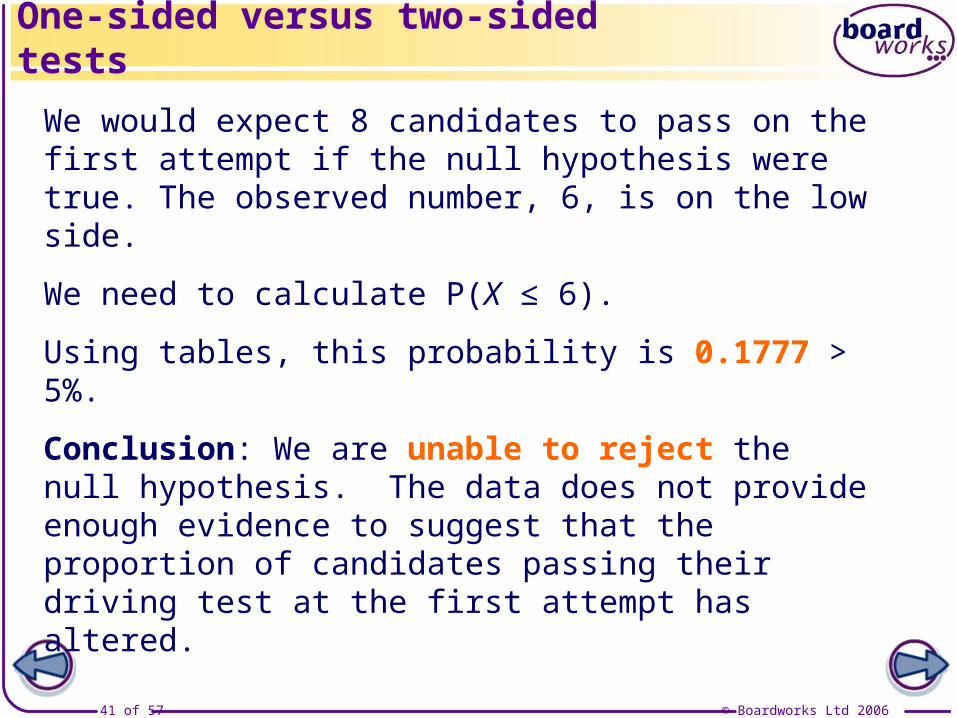
We would expect 8 candidates to pass on the first attempt if the null hypothesis were true. The observed number, 6, is on the low side.
We need to calculate P(X ≤ 6).
Using tables, this probability is 0.1777 > 5%.
Conclusion: We are unable to reject the null hypothesis. The data does not provide enough evidence to suggest that the proportion of candidates passing their driving test at the first attempt has altered.
One-sided versus two-sided tests

© Boardworks Ltd 200642 of 57
Introduction to sampling
Introduction to hypothesis testing
Chocolate tasting practical
One-sided hypothesis tests
One-sided versus two-sided tests
Critical regions
Hypothesis tests and critical regions
Co
nte
nts
© Boardworks Ltd 200642 of 57
Critical regions

© Boardworks Ltd 200643 of 57
Example 1: Police records show that 25% of the vehicles using a stretch of road exceed the speed limit. A new speed camera is installed. The police wish to find out whether this has led to a reduction in the proportion of drivers speeding.
The police sample 20 cars driving along the stretch of road.
Critical regions
The critical (or rejection) region for a hypothesis test is the range of values for which the null hypothesis could be rejected.
a) Find the critical region for a test carried out at the 5% significance level.
b) Comment on the implications of the test if the police find 2 speeding drivers.
© Boardworks Ltd 200644 of 57
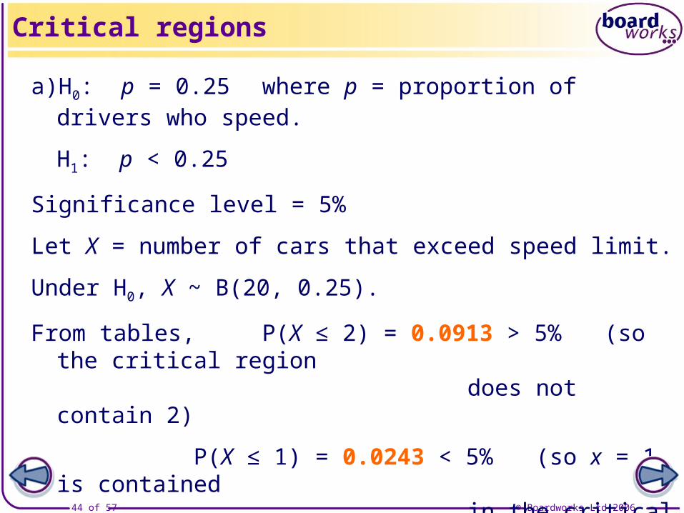
a) H0: p = 0.25 where p = proportion of drivers who speed.
H1: p < 0.25
Significance level = 5%
Let X = number of cars that exceed speed limit.
Under H0, X ~ B(20, 0.25).
From tables, P(X ≤ 2) = 0.0913 > 5% (so the critical region
does not contain 2)
P(X ≤ 1) = 0.0243 < 5% (so x = 1 is contained
in the critical region).
Thus, the critical region for the test is x ≤ 1.
Critical regions
© Boardworks Ltd 200645 of 57
b)The actual number of speeding motorists is 2.
This number is not contained within the critical region.
Therefore we cannot reject the null hypothesis at the 5% level. The evidence does not support the theory that the proportion of motorists that speed has changed.
Critical regions

© Boardworks Ltd 200646 of 57
Examination style question: A gardener knows from past experience that 80% of the runner bean seeds that he plants will germinate. He is forced to switch to a different brand of seed. He wants to find out whether this has led to a change in the germination rate of his runner beans.
He plants 25 seeds. Let X represent the number of seeds that germinate.
Find the critical region for a hypothesis test carried out at the 10% significance level.
Critical regions
© Boardworks Ltd 200647 of 57
Solution:
H0: p = 0.8 (p = proportion of seeds that germinate).
H1: p ≠ 0.8
Significance level = 10% (5% for each tail).
Under H0, X ~ B(25, 0.8).
There will be two parts to the critical region, one corresponding to each tail of the test.
Lower tail: Using tables, P(X ≤ 17) = 0.1091 > 5%
P(X ≤ 16) = 0.0468 < 5%
Therefore the lower part of the critical region is x ≤ 16.
Critical regions
© Boardworks Ltd 200648 of 57
Upper tail: P(X ≥ 23) = 1 – P(X ≤ 22)
= 1 – 0.9018 = 0.0982 > 5%
P(X ≥ 24) = 1 – P(X ≤ 23) = 1 – 0.9726 = 0.0274 < 5%
Therefore part of the critical region for the upper tail is x ≥ 24.
Combining these two parts, the critical region for the whole test is
x ≤ 16 or x ≥ 24.
Critical regions

© Boardworks Ltd 200649 of 57
Introduction to sampling
Introduction to hypothesis testing
Chocolate tasting practical
One-sided hypothesis tests
One-sided versus two-sided tests
Critical regions
Hypothesis tests and critical regions
Co
nte
nts
© Boardworks Ltd 200649 of 57
Hypothesis tests and critical regions
© Boardworks Ltd 200650 of 57
The steps for performing a hypothesis test on the value of a Poisson mean are the same as for a binomial probability:
Step 1:
Step 2:
Step 3:
Step 4:
Step 5: Make a conclusion in the context of the problem.
Write down the null and alternative hypotheses and state the significance level of the test.
Write down the distribution of the random variable assuming that the null hypothesis holds.
Find the probability of obtaining results at least as extreme as those actually recorded – this probability is called the p-value.
Compare the p-value with the significance level and decide whether to reject the null hypothesis or not.
Hypothesis tests on a Poisson mean
© Boardworks Ltd 200651 of 57
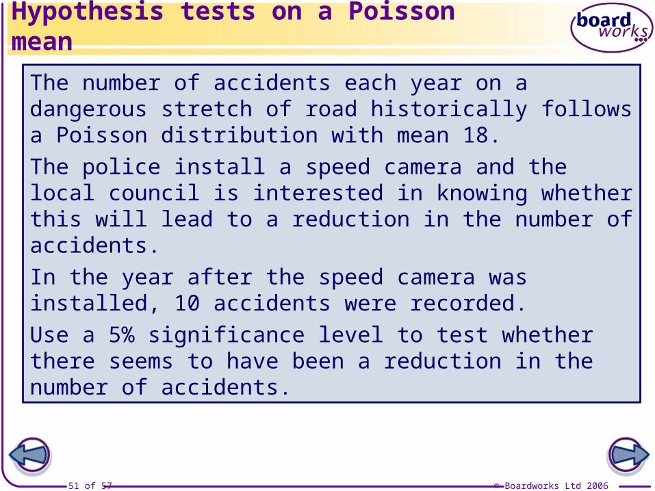
The number of accidents each year on a dangerous stretch of road historically follows a Poisson distribution with mean 18.
The police install a speed camera and the local council is interested in knowing whether this will lead to a reduction in the number of accidents.
In the year after the speed camera was installed, 10 accidents were recorded.
Use a 5% significance level to test whether there seems to have been a reduction in the number of accidents.
Hypothesis tests on a Poisson mean
© Boardworks Ltd 200652 of 57
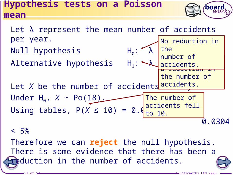
Let λ represent the mean number of accidents per year.
Null hypothesis H0: λ = 18
Alternative hypothesis H1: λ < 18
Let X be the number of accidents in a year.
Under H0, X ~ Po(18).
Using tables, P(X ≤ 10) = 0.0304
0.0304 < 5%
Therefore we can reject the null hypothesis. There is some evidence that there has been a reduction in the number of accidents.
Hypothesis tests on a Poisson mean
There has been a reduction in the number of accidents.
No reduction in the number of accidents.
The number of accidents fell to 10.
© Boardworks Ltd 200653 of 57
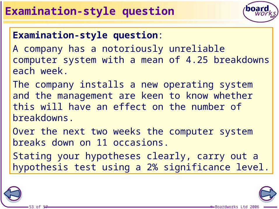
Examination-style question:
A company has a notoriously unreliable computer system with a mean of 4.25 breakdowns each week.
The company installs a new operating system and the management are keen to know whether this will have an effect on the number of breakdowns.
Over the next two weeks the computer system breaks down on 11 occasions.
Stating your hypotheses clearly, carry out a hypothesis test using a 2% significance level.
Examination-style question

© Boardworks Ltd 200654 of 57
Let λ represent the mean number of breakdowns per week.
Null hypothesis H0: λ = 4.25
Alternative hypothesis H1: λ ≠ 4.25
Let X be the number of breakdowns in a two week period.
P(X ≥ 11) = 1 – P(X ≤ 10) = 1 – 0.7634 (using tables)
0.2366 > 1%
Under H0, X ~ Po(8.5).
= 0.2366
Therefore we cannot reject the null hypothesis.
Examination-style question
This is a two-sided test.
There is no evidence that there has been a change in the mean number of breakdowns.
The test is 2-sided, so we compare the p-value with half the significance level.
© Boardworks Ltd 200655 of 57
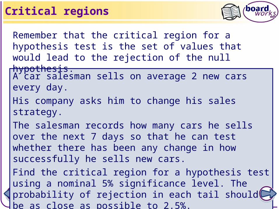
A car salesman sells on average 2 new cars every day.
His company asks him to change his sales strategy.
The salesman records how many cars he sells over the next 7 days so that he can test whether there has been any change in how successfully he sells new cars.
Find the critical region for a hypothesis test using a nominal 5% significance level. The probability of rejection in each tail should be as close as possible to 2.5%.
Remember that the critical region for a hypothesis test is the set of values that would lead to the rejection of the null hypothesis.
Critical regions
© Boardworks Ltd 200656 of 57
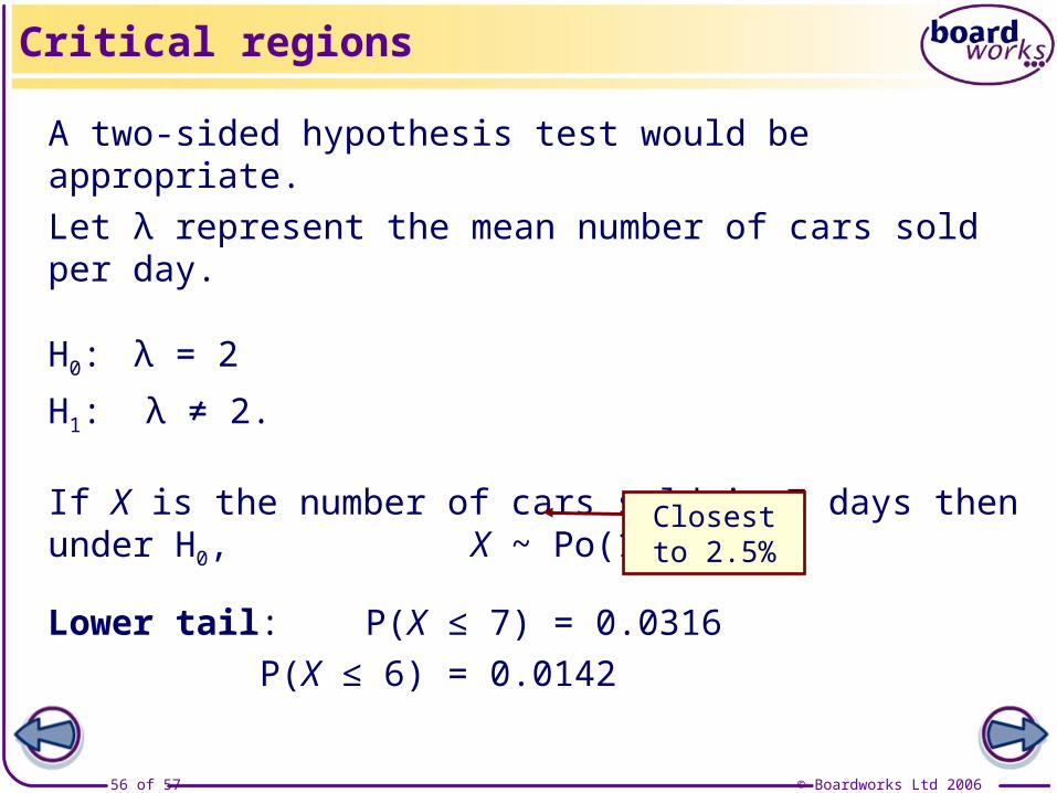
A two-sided hypothesis test would be appropriate.
Let λ represent the mean number of cars sold per day.
H0: λ = 2
H1: λ ≠ 2.
If X is the number of cars sold in 7 days then under H0, X ~ Po(14).
Lower tail: P(X ≤ 7) = 0.0316
P(X ≤ 6) = 0.0142
Critical regions
Closest to 2.5%
© Boardworks Ltd 200657 of 57
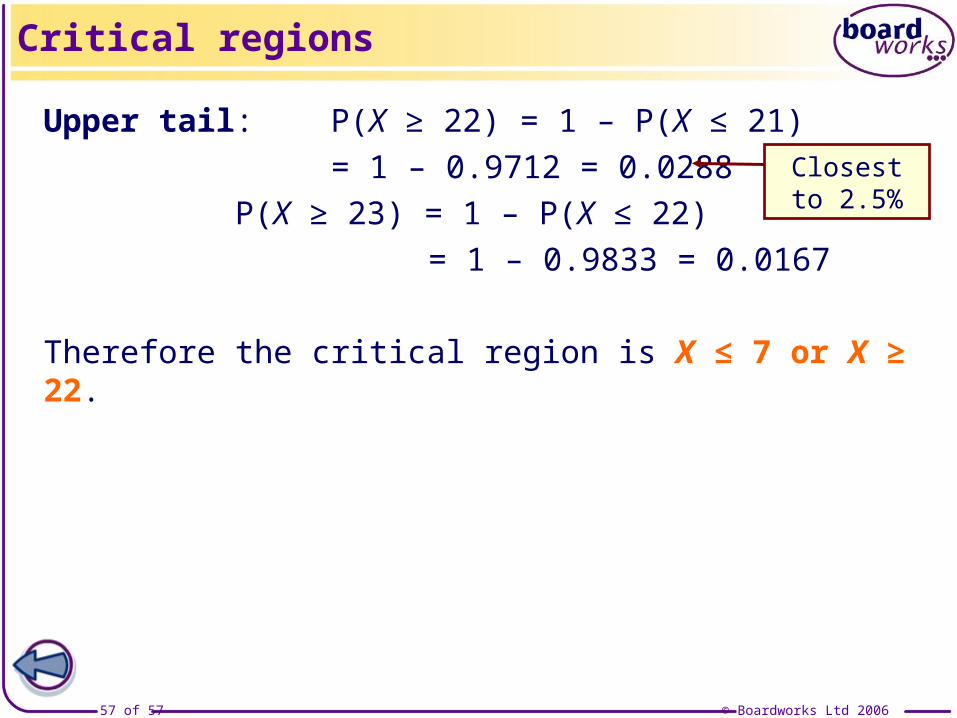
Upper tail: P(X ≥ 22) = 1 – P(X ≤ 21)
P(X ≥ 23) = 1 – P(X ≤ 22)
= 1 – 0.9833 = 0.0167
Therefore the critical region is X ≤ 7 or X ≥ 22.
= 1 – 0.9712 = 0.0288
Critical regions
Closest to 2.5%
Related Documents


