RIGHT: URL: CITATION: AUTHOR(S): ISSUE DATE: TITLE: Estimation of Raindrop Size Distribution from Spaceborne Radar Measurement( Dissertation_全文 ) Kozu, Toshiaki Kozu, Toshiaki. Estimation of Raindrop Size Distribution from Spaceborne Radar Measurement. 京都大学, 1992, 博士(工学) 1992-01-23 https://doi.org/10.11501/3086462

Welcome message from author
This document is posted to help you gain knowledge. Please leave a comment to let me know what you think about it! Share it to your friends and learn new things together.
Transcript

RIGHT:
URL:
CITATION:
AUTHOR(S):
ISSUE DATE:
TITLE:
Estimation of Raindrop SizeDistribution from SpaceborneRadar Measurement(Dissertation_全文 )
Kozu, Toshiaki
Kozu, Toshiaki. Estimation of Raindrop Size Distribution from Spaceborne RadarMeasurement. 京都大学, 1992, 博士(工学)
1992-01-23
https://doi.org/10.11501/3086462

EsuvtATIoN or RaINDRop Szn DlsrnIBUTIoN
FROM
SpncrsoRNE Rnpen MBaSUREMENT
Toshiaki Kozu
Submitted to the Graduate School of Engineering
in partial fulfillment of the requirements
for the degree of Doctor of Engineering at Kyoto University
August I99l
EsrnrATIoN op ReINDRop Szn DISTnIBUTIoN
FROM
SpncgBoRNn, RnpAR MBnSUREMENT
August I99l
Toshi鍬 こi Kozu

AgSTRACT
The growing importance of global climate change monitoring has given rise in recentyears to the development of rainfall measuring systems from space. Microwave sensors shouldplay an important role for such systems. Radars are particularly important since they work
regardless of background (Land/ ocean) and provide the information on vertical storm
structures. For "quantitative" measurements, however, more studies need to be done to reduce
measurement errors. The purpose of this study is to develop a method for spaceborne radars to
estimate parameters of raindrop size distribution (DSD) and thereby to reduce the error due to
the uncertainty in DSD that is known as a major non-instrumental error source in radar rainfall
measurements. Estimating the DSD parameters should lead not only to a better estimate of a
meteorological quantity of interest but to a deeper understanding of precipitation processes.
It is well known that dual-parameter (DP) radar measurements can reduce the rain rate
estimation error significantly. This is because the DP measurement can provide two indepen-
dent DSD paftrmeters in conffast with single-parameter (SP) measurements providing only one
DSD parameter. The dual-polarization (Zoil technique is a promising method to make a
"complete" (i.e. for each range gate basis) DP measurement for ground-based radars. For
spaceborne radars, however, it is difficult to perform such complete DP measurements because
of the reduced Znn measurement sensitivity (due to the down-looking observation geometry)
and limitations in mass, size and electric power. In this study, therefore, the combination of a
radar reflectivity profile and a path-integrated attenuation derived from surface return or
microwave radiometers, which will be available from most spaceborne systems, is employed
for the DSD estimation. To discuss this type of DP measurement generally, a new concept,
"semi-dual-parameter" (SDP) measurement is proposed together with a "t\ryo-scale" DSD model
the parameters of which can be estimated from an SDP measurement. An algorithm is pro-
posed for the SDP measurement to estimate the DSD paftrmeters and then to derive rainfall rate.
In order to test the perforrnance of various radar rain rate estimation methods, a large
amount of DSD data measured on the ground by a disdrometer are employed after examining
the accuracy and the validity of the disdrometer data for radar rainfall remote sensing studies.
The test result indicates that the SDP measurement has an accuracy in rain rate estimation from
2 to 4 times better than the SP measurement depending on the range resolution in the
affenuation measurement.
The perfonnance of the SDP measurement is also tested using the data obtained from a
dual-frequency airborne radar experiment. The SDP measurement is constructed by the
combination of an X-band radar reflectivity profile and either X- or Ka-band path attenuation
obtained from sea-surface echo. The validity of the estimated DSD parameter and of the derived
rain rate is conf,rrmed by a consistency check using the measured Ka-band radar reflectivities.
Based upon the results obtained in this study, ? consideration is given of general
suategies for processing spaceborne radar data to generate accurate and useful rainfall
parameters. Discussion is also made on the usefulness of the DSD estimation method
developed in this study to improve a wide range of radar rainfall measurements from space.
1
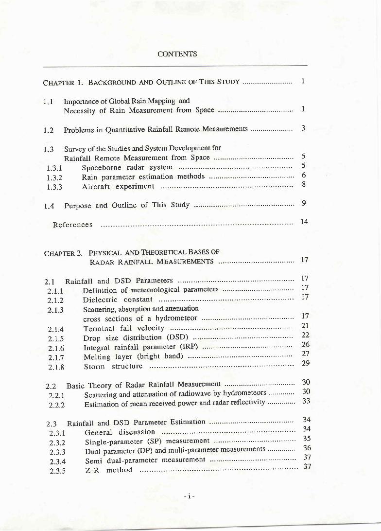
CONπ NTS
CHegrEN 1. BACKGROUND AND OUTTNITE OF THIS STUNY
1. 1 Importance of Global Rain Mapping andNecessity of Rain Measurement from Space 1
L.2 Problems in Quantitative Rainfall Remote Measurements 3
1.3 Survey of the Studies and System Development for
Rainfall Remote Measurement from Space
1.3.1 Spaceborne radar system
I.3.2 Rain parameter estimation methods
L.3.3 Aircraft exPeriment
1.4 Purpose and Outline of This Study
Re fere nce s
CHeprPN 2. PHYSICAL AND TIIEORETICAL BNSES OT
RADAR RRIXTEI-I MEASUREMENTS
2.I Rainfall and DSD Parameters
z.I.L Definition of meteorological parameters
2 . I . 2 D ie lec t r i c cons tan t . . .
2.I.3 Scattering, absorption and attenuation
cross sections of a hYdrometeor
2.I.4 Terminal fall velocitY
2.1.5 Drop size distribution (DSD)
2.L.6 Integral rainfall parameter (IRP)
2.1..7 Melting layer (bright band) """"':"2.L.8 Storm structure
2.2 Basic Theory of Radar Rainfall Measurement
Z-Z.I Scattering and attenuation of radiowave by hydrometeors
2.2.2 Estimation of mean received power and radar reflectivity --..--.....-.-
2.3 Rainfatl and DSD Parameter Estimation
2.3.L General discussion
2.3.2 Single-parameter (SP) measurement
2.3.3 Dual-parameter (DP) and multi-parameter measurements .""""""'
2.3.4 Semi dual-parameter measurement
2.3.5 Z-P. method
5568
9
L4
17
7
7
7
‐7
2‐
22
26
27
29
0
0
3
3
3
3
34
34
35
36
37
37
2.3.62.3.72.3.82.3.9
Appendix
Surface reference target (SRT) methodRange profiling methods for attenuating frequency radarDSD est imat ion methods . . . .Mirror image method
2-L Bright band model
9
0
3
4
1
3
4
4
3
6
4
4Re fere nce s
CI・IAPTER 3.■E USE OF GROIIND―MEASURED DSD DATA FOR
THE STUDY OF RADAR RAINFALL RE口 RIEVALS.… …̈………….
3.l The Joss― Waldvogel Type E)isdrometer 。 ¨̈ “̈" “̈̈ “̈̈ "̈¨̈ ““̈ ¨̈
3.1.l lnstrument description .¨ ………………̈ ………………………………………………・
3.1.2 Sampling error .¨ ¨̈ …̈…………………・・̈……………………………………………
3.1.3 Sensitivity at small diameter channels .""¨ ".・̈¨̈ ¨̈ ¨̈ ・̈・・・"“"
3.2 DSI) Mcasurement at Kashima .¨ ¨̈ ¨̈ “̈ ¨̈ ¨̈ ¨̈ ¨̈ ¨̈ ¨̈ 。̈̈ ・̈̈¨
3.3 Analysis of Slant―Path Rain Attenuation using Disdrometer Data。………¨
3.3.l Event―scale attenuation ratio properties .¨"̈ “̈"¨̈ ¨̈ ……………̈ "
3.3.2
3.4 Ku― band FM― CW Radar Calibration using Di鹸 ometer Data.… .. …̈ “̈・
3.4.1 0utline of the FM― CW radar .¨ ¨̈ “̈̈ “̈ ¨̈ ・̈・̈¨̈ “̈̈ ・̈・̈¨̈
3.4.2 Calibration method .¨ ¨̈ ………………̈ ¨̈ ¨̈ ¨̈ ¨̈ ¨̈ ……………………・
3.4.3 Result of the calibration .¨ ¨̈ ¨̈ …̈……・・̈¨̈ ¨̈ "¨¨̈ ¨̈ …̈………
3.5 Conclusions 。 ¨̈ ¨̈ ¨̈ ¨̈ …̈……………………………………………………………………
Appendix 3-l De五 vation of radar equation for the Ku―band FM― CW radar.¨ .̈.
References ◆ ….……………。̈¨̈ ¨̈ ¨̈ ・・̈ ・̈・…………̈ …………・・…・・“・̈ ・̈・…。…。̈・
CHAPTER 4. STATISTICAL PROPERTIES OF DSE)PARAMEπ RS.¨ ¨̈ ¨̈ “̈ ・̈ 77
4。l DSE)Models and thc Parameter Estimation Methods.¨ ““。。̈¨̈ ¨̈ “̈̈ ・ 77
4.2 Statistics of DSD Parameters .¨ …………………………………。・̈¨̈ ¨̈ …̈…。・̈ ̈ 81
4.3 1nterrelations among】 DSE)Parameters and】 DSI)Momcnts.¨ ¨̈ “̈̈ "¨̈ 86
5‐
5‐
5‐
53
54
55
57
59
63
65
65
67
7。
72
73
75
11

4.3.1 Rain rate and Z factor dependences of DSD parameters ....... 864.3.2 Correlations between DSD parameters and between IRPs 894.3.3 Relations between IRPs
4.4 Tests of Rain Rate Estimation Accuracy by SP and DP Measurements ......
4 . 5 E r ro r Ana l ys i s . . . .
4.6 Conclusions
Appendix 4-1 Derivation of DSD parameters
References
92
98
r02
106
CHAPTTR 5. SDP MEASUREMENT AND TWO-SCALE DSD MODEL 110
5 .1 Concep t . . 110
5.2 Two-scale Model and Relations between IRPs
5.3 Proper Two-Scale Model: Empirical Evidence LI4
5.4 Simulation of SDP Measurements 1 18
5.4.1, Simulat ion method 118
5.4.2 Simulation result; rain rate profile LZI
5.4.3 Estimation of path-averaged rain rate L25
5.5 Validity of the Two-scale Model 125
5.6 Conclusions ' L28
Appendix 5-1 preliminary analysis of rain-type dependence of Z-Rrelation 130
References 133
CuEprER 6. ARSORI'TE RADAR RNIUT.NLL MEASUREMENT ....... T34
6.1 Airborne Radar/Radiometer 134
6.2 Outline of the ExPeriment L39
6.3 Radar Equation and Processing of Level "7nro" Data L42
08 ”
111

6.4 External Radar Calibration
6.5 Conc lus ions
Appendix 6.1 Parameters in the radar equation for the T-39 experiment ...........
Re fere nce s
Ctrnplen 7. ExpN,RIPMNTAL TESTS OF SEMI DUAL.PARAMETERMEASUREMENT 150
7.L Methods of the Test and the DSD Model 150
7 . l .L General discussion 150
7.L.2 Description of the power-law approximation method 154
7.L.3 Melting layer attenuation 158
7 .2 Results and Discussion . 162
7.2.L Spatial trend of N6 L62
7.2.2 Consistency with Ka-band Ze 163
7 .2.3 Error sources L70
7.2.4 Effects of errors in Zm and A5p on Ng estimation ....
7 .3 Conclusions
Reference s 174
CTTNPTEN 8. CONSPBNATION OF ITADAR TTAINFALL RETRIEVAL
AICONTTHMS FROM SPECE L75
8.1 Estimating Apparent Effective Radar Reflectivity Factor (Zm) L75
8.2 Estimating Rain Rate and Liquid Water Content .......... L77
8.2.1 Z-F. and Z-W methods .... I77
8.2.2 Surface reference target (SRT) method I78
8.2.3 Range profiting of R and I{z L79
8.2.4 Non-uniform beam filling (NUBF) effects 179
8.2.5 Limitations of the Z-R and SRT methods 180
8.3 Usefulness of SDP Measurement Estimating DSD 180
8.4 Radar Data Processing Flow I82
“ ″
8
9
4
4
1
2
7
7
lV

8.5 Issues to Develop Spaccborne Radar Algorithms .......8.5.1 Modcling studies ........8.5.2 Test and validation of the algorithms
References
184184185
t87
Acknowledgments
List of publications
8
3
8
9

LIsT oF TABLES
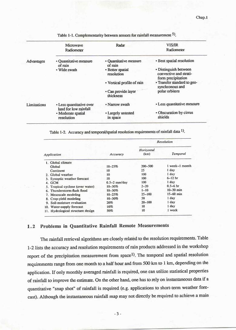
Table 1-1 Complementarity between sensors for rainfall measurement..... 3
Table 1-2 Accuracy and temporaVspatial resolution requirements of rainfall data.... 3
Table 1-3 Major parameters of proposed TRMM radar 6
Table 2- 1 Definitions and units of meteorological and radar quantitiesused in this thesis.
Table 2-2 Complex refractive indices of water and ice for several
radar frequencies
Table2-3 Moment approximation of typical IRPs (IRP - C Mn)...........
18
9
7
1
2
Tablc 2-Al
Table 3-1
Table 3-2
Table 3-3
Parameters of the bright band particle model and refractive indices........
Diameter range of the disdrometer analyzer channels and drop
terminal velocity at the geometrical center of the channels
Parameters for up-link and down-link attenuation measurements. -. -- - -.- -
Summary of the event attenuation ratio (ARev) analysis
52
8
2
5
6
85
44
89
96
Table 3-4 Major parameters of FM-CW radar.... 66
Table 4-1 Statistics of DSD parameters derived from disdrometer data
Tab\e 4-2 Rain-rate dependence of DSD parameters for two-parametergamma, and three-parameter gamma and lognormal models................
Table 4-3 Important IRP relationships derived from linear regressions
between the logarithms of IRPs.-..-
Table 4-4 RMS dB errors to estim ate Z from R, and & from R using
the IRP relations shown in Table 4-3----- 97
Table 4-5 Results of zeroth moment (Md estimation from DP
measurements combining M 6 and M +-. LOz
Vl
Table 5-2
Table 5-Al
Table 6‐1
Table 6-2
Table 6‐3
Table 64
Summary of R and W estimation crror.... 104
Coefficient a and exponent b in the rain parameErrelationships for the gamma DSD model...
A result of path-averagcd rain rate estimation.........
Statistics of the coefficient a and the exponent b in Z-R re1aion...........
Major specifications of NAS An49 aircraft.
Major system parameters for the T-39 experiment........
Summary of the T-39 experiment, fall 1988.....
Meteorologicat data during the flights,
‐4
2
32
34
38
39
fal l 1988 measured at WFF.... --...--.....
Table 7-1 Coefficiens of the power-law reliations for some Ng values obtained
by linear regression of logarithms of k,Ze,R, and A va1ues............... 155
― Vll ―

LIST OF FIGURES
Figure 1- 1 Flowchart of this thesis. I 1
Figure 2- 1 Terminal fall velocity of raindrops using different equations,
and comparison of rain rates calculated from ground-measured
DSDs using terminal velocities vUr(D) and vtu(D)- 2L
Figxe 2-2 Examples of natural DSD measured by a disdrometer.... 24
Figure 2-3 Regression results of the relation between logarithms of os and D....... 25
Fig;ne2-4 Examples of vertical radar reflectivity profile.......... 28
Figure 2-5 Difference in Ze factots of the spherical drop model
and the deformed drop model at 10 GHlz and 35.5 GH2...... 32
Figure 2-6 Concept of rain parameter estimation by means of
remote sensing techniques.
Figwe 2-7 Distributions (weighting functions) for several moments of DSD
Figure 2-8 A comprehensive plots of Z-R relationships
on a rain-Parameter diagram
Figure 3- I Schematic representation of the transducer
for the Joss-Waldvogel disdrometer.-
Figure 3-2 Distribution of normalizel m (rnJn) of
Poisson-distributed random process.
Figure 3-5 Histogram of the difference between IRPs calculated with
the original and modified disdrometer data......
Figure 3-6 I-ocation of the disdrometer and other related instmments at Kashima---
34
36
38
53
52
Figure 3-3 Effect of sampling elror on calculated Z va\ue 54
Figure 3-4 Example of disdrometer data modification. 56
56
Vlll
57
Figure 3-7 Example of the determination of "event" attenuation ratio (M"r)
for measured and disdrometer-derived attenuation values.......... 60
Figure 3-8
Figure 3-9
Figure 3- 10
Figure 3- I I
Scattergrams of measured versus DM-derived AR*;
and comparison of correlations between measured and
DM-derived AR*'s and between ARerr's measured and
estimated with the assumption of Marshall-Palmer mode1.................
Comparison of measured and DM-derived attenuation ratios....
Ratio of attenuation cross sections at two d.ifferent frequencies
(QtR) as a function of drop diameter.....
Results of slant-path attenuation ratio calculation: rain-only,
bright-band-only, and total (including gas attenuation)-.-....
61
62
6 4
6 4
Figure 3-12
Figure 3-L3
Figure 3-L4
Flowchart of radar calibration.. 68
Example of disdrometer-measured DSDs.-- 68
69
73
80
Attenuation coefficient vs. Ze relationships
measured in Event 1 and Event 2.
Figure 3-15 F value versus RMS deviation between Appp and Apv
Figure 3-L6 Comparison of radar-derived rain rate on the BSE path with
ground-measured rain rate.
Figure 3-A1 Scattering volum e LV for the calculation of radar received power........
Figure 4- 1 Examples of model fining of measured DSD with the higher-order
moment est imat ion
71
71
Figure 4-2 Histogram of exponential DSD model parameters-...-.-. 82
Figure 4-3 Histogram of gamma DSD model parameters"""" 83
Figure 4-4 Histogram of lognormal DSD model parameters"' 84
Figure 4-5 Cumulative distribution of Ns of the exponential DSD model-- 86
lX
Figure 4-6 Rain rate dependences of the exponential DSD parameters................ 87
Figure 4-7 Rain rate dependences of the gamma DSD model parameters............. 88
Figure 4-8 Rain rate dependences of the lognormal DSD model parameters.......... 88
Figure 4-9 Scattergrams of the gurmma DSD model parameters;
nt vs. log Ns and log (m+4) vs. log n.... 9L
Figure 4- 10 Scattergnms of the girmma DSD model parameters;
log N1 vs. log A and log N1 vs. m... 9I
Figure 4-lL Scattergrams of rain rate vs. several moments........... 94
Figure 4-LZ Correlation coefficients betwern moments of DSD; theoretical
calculation and those obtained from disdrometer data 95
Figure 4-L3 Seasonal variation in the relation between Z factor and rain rate
derived from the 2-year disdrometer data...... 97
Figure 4-I4 Comparison of rain rate estimates by an SP measurement,
a DP measurement, and TP measurements..- 99
Figure 4-15 Dependence of rain rate estimation accuracy on the gamma DSD
parameter m and on the lognormal DSD parameter o...... 100
Figure 4-16 Rain rate and LWC estimation error caused by errors inZ-factor
and attenuation measurements, and in natural DSD fluctuation........... 105
Figure 5- 1 Concept of DP, SDP and SP measurements using radar reflectivity
factor (Z) and, microwave attenuation (k) for rainfall profiling I 11
Figure 5-2 Illustration showing examples of SDP measurement by a spaceborne
radar, and by a combination of ground-based radar and a raingage...... llz
Figure 5-3 Event-scale Z-R relationship derived from disdrometer data 115
Figure 5-4 Concept of principal component analysis to see the proper
two-sca le DSD model - - 116

Figure 5-5 Argument of the first principal component of two moments
obtained from event-scale analysis ll7
Figure 5-6 Concept of SDP measurement simulation with disdrometer data 119
Figure 5-7 Example of estimates of "path-averaged" N6
and corresponding A Profile. . lzt
Figure 5-8 Comparison of rain rate estimation results by a DP measurement,
two SDP measurements, ild an SP measurement..... I22
Figure 5-9 Nr dependence of rain rate estimation accuracy L23
Figure 5- 10 Mean and standard deviation of correlation coefficients between
logarithms of Ns and Z,Nr andZ, and A andZ..-- L24
Figure 5- 1 1 Correlations between Ng derived from a DP measurement and
that derived from SDP measurements with Nr - 2 and 32...-..... L26
Figure s-LZ Dependence of o5 / o1 ratio on N7. L27
Figgre 5-A1 Rain-type classification method 130
Figure 5-AZ ScattergRms of rain-type vs. mal(. rain rate, andof rain-type vs. P ...-. 131
Figure 5-A3
Figure 6- 1
Figure 6-2
Figure 6-3
Figure 6-4
Scattergrams of F ut. cr for typical stratus and cumulus rains L32
NASA T-39 aircraft at WFF and instruments installed on the aircraft.... 135
Block diagram of the instruments for the T-39 experiment.-...... L37
Data acquisition timing chart of the dual-frequency radar/radiometer...-. 137
Example of 3-D plot of X-band and Ka-band Zm ptoftles---.-.-.. I4O
Figure 6-5 Example of contour plots of Zm l'41
Figure 6-6 Ground track of the flight on October 21, 1988,
and the location of raingages.--.. L45
Xl
Figure 6-7 Time trend of rain rates measured by raingages
and the timing of aircraft passage 145
Figure 6-8
Figure 7- I
FigneT-2
Figure 7-3
Conelation between rain rates as measured by raingages
and as estimated by the X-band radar using a MP Ze-R
relation and the calibrated radar system constant L46
Concept of estimating DSD parirmeters,Ze and
rain rate profiles by SDP measurement..... 153
Flowchart of DSD estimation procedure......... 156
Storm model used to calculate path-attenuation
and path-averaged rain rate from Zm profile.. L59
Figure 7-4 Comparisons of Z-way path attenuations derived from surface
echoes, the estimated Ng, and the corresponding X-bandZm
profile on October 28, 1988. 160
Figure 7-5 The same as Fig.7-4 except on November 1, 1988... 160
Figure 7-6 Examples of X- and Ka-band zm and ze ptoflles.. l&
Fignre 7-7 Scattergram of the ratio of retrieved Ka-band Ze to
X-band Ze (KatX Ze ratio) versus estimated NO value.... 165
Figure 7-8 Comparison of path-averaged rain rates calculated
from X-band and Ka -band Ze profiles L66
Figure 7-9 Comparison of rain rate profiles calculated from
X-band and Ka-band Ze profiles L67
Figure 7 -lO Differences between the logarithm s of R7a and R716qSD
and between the logarithms of R7a and R71s,MP
as a function of range. L69
Figure 8-1 A flowchart of spaceborne radar data processing..... 183
Xll
APR
BEST
BSE
CRL
CS
DM
DP measurernent
DSD
DSRT
岬
EOF
FOV
GEWEX
GSFC
H―B solution
HPBW
IRP
J―D distribution
JEM
J―T distribution
J―W distribution
LDR
LWC
MARS
MLE
M―N model
MoM
MP distribution
NASA
N/N model
NUBF
P―P
SDP Ineasllrement
SP measllrernent
SRT method
M
TOGA
T measurement
… R
帥
WCRP
W F F
List of Acronyms
Average Probability RatioBilan Energetique du Systeme TropicalBroadc astin g Satellite for Experim en tal p urpose sCommunications Research LaboratoryCommunication S atelliteDisdrometerDual-Parameter m easuement(Rain) Drop Size DistributionDual-wavelength Surface Reference Target method
Dual Wavelengths TechniqueEmpirical Orthogonal FunctionField-of-ViewGlobal Energy and Water Cycle Experiment
Goddard Space Flight CenterHitschfeld-Bordan solutionHalf-Power Beam WidtttIntegral Rain ParametersJoss-Drizzle distributionJapanese Experimental ModuleJoss-Thunderstorm distributionJoss-Wide spread distributionLinear Depolarization RatioLiquid Water ContentMicrowave Airborne Rain Scatterometer/radiometer
Maximum Likelihood EstimationModified Nishitsuj i modelMethod of MomentMarshall-Palmer distributionNational Aeronautics and Space Administration
NoncoalescenceA.lonbreakup model
Non-uniform Beam FillingProbability den sity fu nction
Pruppacher-Pitter (raindrop shape)
Semi-D ual-Parameter measuremen t
S ingle-Parameter measurementSurface Reference Target method
TRMM Microwave ImagerTropical Ocean and Global Aunosphere
Triple-Param eter Meas urem ent
Tropical Rain Mapping RadarTropical Rainfall Measuring Mission
World Climate Research Program
Wallops Flight Facility
Xlll

Chap.l
CHAPTER l.BACKGROUND AND OUTLINE OF THIS STuDY
l。l lmportance of(Global lRain Mapping and
Necessity of Rain Measurement from Space
Rainfalt, the major water flow from atmosphere to land and to ocean, is a life-giving
resource for Earth biosphere. It sometimes exhibits dangerous anomalies (flood/drought), and
appears as destnrctive storms, however. Rainfall distribution is also one of the most important
and least-known parameters related to the global hydrological cycle, which is associated with
energy fluxes between atmosphere and land/ocean and therefore couples various components
of the global climate systeml-7). Knowledge of the variation of global rainfall distribution is
therefore crucial to understand and to predict the gtobal climate change and weather anomalies.
At present, reliable rainfall data are available only from limited developed countries
mainly located around mid-latitudes. In particular, little is known about the rainfall over vast
ocean areas where no rain gage or weather radar exists. Therefore, satellite remote sensing is
recognized as the most effective and probably the only way to measure global rainfall-
However, the rainfall is also recognized as one of the hydrological and meteorological
paramerers most difficult to measure mainly because of its high spatial and temporal
variabilities. Although spaceborne visible and infrared sensors have sufficiently high spatial
resolutions, they can not penetrate cloud. Although microwave sensors can directly "see" the
rain below cloud cover, spaceborne sensors that have been flown to date (i.e., all radiometers)
have had only very crude spatial resolutions. The lack of adequate spatial resolution makes the
quantitative measurement difficult l'3).
yet, because of its important role in global hydrological cycle and climate, a number of
studies of rainfall measurement from space have been attempted using visible/infrared and
microwave radiometers onboard several remote sensing satellites. In spite of the problem of
spatial nonuniformity of rain within their field-of-view (FOV), microwave radiometers
operating at 10 to 20 GHzhave been recognized as promising tools for estimating vertically
integrated rain rate over the oceans8). Microwave absorption by raindrops causes an increase in
brightness temperarure from the cold ocean background. Higher frequency (> 37 GIJz)
radiometers are also useful to estimate the upper structure of rain storms since the brightness
rcmperature is sensitive to scattering by ice particles aloftS). Algorithms combining multi-
frequency radiometers ranging from 18 to 90 GHz have also been proposed9)- Such

Chap.l
combination may also provide a crude rainfall profile. Clearly, there are several weak points in
the microwave/millimeter wave passive sensors; there is no range resolution capability except
for the crude profiles obtained from the multi-frequency inversion technique, and there is
difficulty in estimating rain rate over land. In this sense, the radar is an excellent instrument
complement to the radiometers.
The capability and the usefulness of radar to observe precipitation were recognized more
than 40 years ago l0). Since its inception, numerous studies have been performed to extend its
ability to discriminate particle typo, to improve rain rate estimation accuracy and to measure
various atmospheric processes. As a result, weather radars are now widely used throughout
the world for weather forecasting, warning, and meteorological and climatological studies.
However, use of the weather radar has been limited to ground-based usage except for some
special-purpose applications of airborne and shipborne radars.
As mentioned above, radars will play a very important role in space-based rainfall
measurements. Potential benefits expected from the radar measurements are:
(1) Unlike the passive microwave sensors, the radar can provide rainfall estimates independent
of the microwave emission properties of the background (land or ocean). The radar measure-
ment is, therefore, especially important over land where the radiometers do not work so well-
(2) The radar has range profiling capability. Data on the vertical storm structure is important
for developing accurate passive microwave rainfall retrievat algorithms, for estimating latent
heat release profile, and for other fundamental atmospheric science studies.
(3) BV utilizing the surface return as a tool to estimate path-averaged rain rate, the radar can
extend the rain rate measurement dynamic range toward ttre higher rain rates.
(a) The storrn structure and rainfall characteristics that are inferred from the radar observation
could be utilized to improve the passive microwave rainfall retrieval accuracy not only for the
rainfall within the radar swath but to outside the radar swath.
(5) The radar data could be combined with the passive microwave data to provide more
accurate rain rate estimates and to infer raindrop size distribution (DSD). The latter can then be
used to estimate the relationships between radar reflectivity and rain rate, and between other
rain-parameters for each observation or each storrn bases, which may further improve the
accuracy of radar algorithms.
Complementarity of the radar and other passive sensors has been well documented in
the litera1s1pl,3,5,8) and is summanz"A,in Table 1-15).
2
Chap.1
Table l-1. Complementarity between sensors for rainfall measurement 5).
R a d a
Adrrantages - Quantitative measure . Quantitative measure . Best spatial resolutionof rain of rain
. Wide swath . Beuer spatial . Distinguish betweenresolution convective and strati-
form precipitation. Vertical profile of rain 'Transfer standard to geo-
synchronous and. Can provide layer polar orbiters
thickness
Limitations .I-ess quantitative over . Narrow swath . Less quantitative measureland for low rainfall
. Moderate spatiat .I-argely unt€sted . Obscuration by cimrsresolution in space shields
Table l-2. Accuacy and temporal/spatial resolution requiremens of rainfall data l).
Resolution
Horizontal
Application Accuracy (km) Temporal
MicrowaveRadiometer
VIS/IRRadiometer
3. Synoptic weather forecast l0
4.GCM
5. Tropical cyclone (over water) lO-30Vo6. Thunderstorm-flash nood l0-30Vo
200-500 1 WeCk-l lnonth
25 1 day
loo l day
loo 6-12 hr
2-20 0.5-6 hr
l-10 10-30■ In
25-100 15-60■ in
1. C)lobal climate
C}lobal
Continent
2. Global weather
7. Mesoscale modeling
8. Cropyield modcling
O.5-2 mm/day 100 | daY
10-25%
10
10
10-25%
10-3磁
9. Soil-moisture evaluation ZOVo10. Water-supply forecast 107o
I l. Hydrological structure design SOVo
50
20-100
10
10
daydaydayweek
L.2 Problems in Quantitative Rainfall Remote Measurements
The rainfall retrieval algorithms are closely related to the resolution requirements. Table
l-2 lists the accuracy and resolution requirements of rain prducts addressed in the workshop
report of the precipitation measurement from spacel). The temporal and spatial resolution
requirements range from one month to a half hour and from 500 km to 1 km, depending on the
applicarion. If only monthly averaged rainfall is required, one can utilize statistical properties
of rainfall to improve the estimate. On the other hand, one has to rely on instantaneous data if a
quantitative "snap shot" of rainfall is required (e.g. applications to short-term weather fore-
cast). Although the instantaneous rainfall map may not directly be required to achieve a main
3

Chap.l
goal of a space mission, such high temporal and spatial resolution data are required to
determine the statistical properties of rainfall, and therefore imponant also to develop statistical
rain-retrieval algorithms. In this srudy, therefore, we focus our attention on the problem of
estimating the high resolution rainfall parameters; rainfall profile or path-averaged quantities.
As described later in this thesis, the quantity that can be measured by rain radar is the
receiver video output voltage, which is digitized and stored on a storage device. By means of
internal and external calibrations, it can be related to the receiver input power and then to a
radar reflectivity factor of rain (called Z or Z-factor; later in this thesis, a more general defini-
tion of Z-factor, Ze will also be used) or a surface scattering cross section (oO). Z-factors and
in some cases o0 are then used to estimate various rainfall parameters such as rain rate and
liquid water contenl The term "quantitative" rainfall remote-sensing is defined as quantitative
estimation of those rainfall parameters required for Earth sciences such as hydrology, clima-
tology and meteorolory, and for microwave or millimeter wave communication engineering.
There are various error sources in the rain parameter estimation:
(1) Absolute radar calibration is required to determine quantitatively theZ-factor and c0 from
the raw radar data.
(2) Relative radar calibration is required to obtain differences in power between two received
signals from which rain attenuation and other rain parameters can be deduced.
(3) Statistical fluctuations in the radar received power cause an error in the estimation of mean
received power. To reduce these fluctuations, a large number of independent samples should
be averaged.
(4) Noise and interference mask rain echoes and cause bias (usually positive) errors. To
diminish this bias error, the noise or interference signal level should be estimated and be
subtracted from the total (signal plus noise or interference) level.
(5) Rain attenuation of the radar signal during propagation between the radar and a radar
scattering volume can cause a negative bias error if a radar equation neglecting the attenuation
is used to estimate the Z-factor. Correction for the attenuation tends to be very unstable and
results in highly elroneous Z-factor estimates-
(6) partial beam filling or nonuniformity of rain within a scattering volume may cause bias
errors due to the non-linear relationships between Z-factor and other rain parameters.
(7) Variation in raindrop size distribution is a major cause of error in rain parameter estimation
4
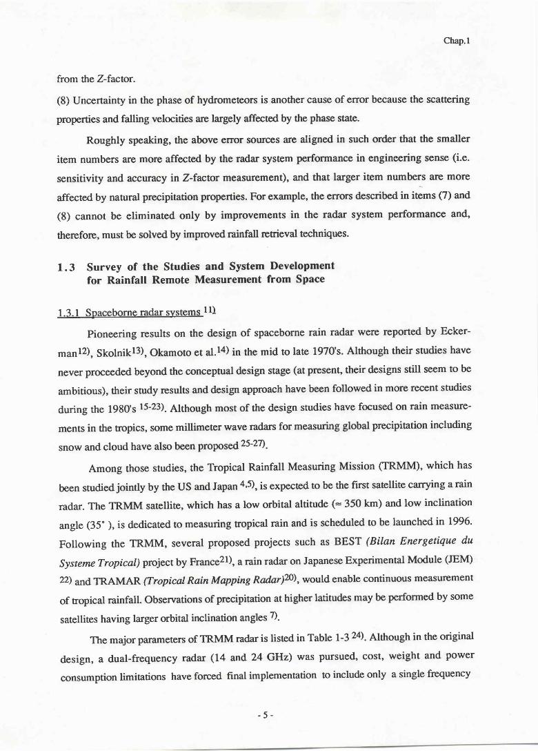
Chap.l
from the Z-factor.
(8) Uncertainty in the phase of hydrometeors is another cause of error because the scattering
properties and falling velocities are largely affected by the phase state.
Roughly speaking, the above enor sources are aligned in such order that the smaller
item numbers are more affected by the radar system performance in engineering sense (i.e.
sensitivity and accuracy in Z-factor measurement), and that larger item numbers are more
affected by natural precipitation properties. For example, the errors described in items (7) and
(8) cannot be eliminated only by improvements in the radar system performance and,
therefore, must be solved by improved rainfall retrieval techniques.
1 .3 Survey of the Studies and System Development
for Rainfall Remote Measurement from Space
1.3.1 Spaceborne radar systems ll)
pioneering results on the design of spaceborne rain radar were reported by Ecker-
manl2), Skolnikl3), Okamoto et al.l4) in the mid to late L970's. Although their studies have
never proceeded beyond the conceptual design stage (at present, their designs still seem to be
ambitious), their study results and design approach have been followed in more recent studies
during the 1980's 15-23). Although most of the design studies have focused on rain measure-
ments in the tropics, some millimeter wave radars for measuring global precipitation including
snow and cloud have also been propos gt25-27).
Among rhose srudies, the Tropical Rainfall Measuring Mission (TRMM), which has
been studied jointly by the US and Japan 4,5), is expected to be the first satellite carrying a rain
radar. The TRMM satellite, which has a low orbital altitude (: 350 km) and low inclination
angle (35" ), is dedicated to measuring tropical rain and is scheduled to be launched in 1996.
Following the TRMM, several proposed projects such as BEST (Bilan Energetique du
Systeme Tropical) project by Fran ce2l), a rain radar on Japanese Experimental Module (IEM)
22) andTRAMAR (Tropical Rain Mapping Radnr)20), would enable continuous measurement
of tropical rainfall. Observations of precipitation at higher latitudes may be performed by some
satellites having larger orbital inclination angles 7).
The major parameters of TRMM radar is listed in Table l-3 24). Although in the original
design, a dual-frequency radar (14 and 24 GIJrz) was pursued, cost, weight and power
consumption limitations have forced final implementation to include only a single frequency
-5

Chap.l
Table I -3. lvlajor parameters of proposed TRMM radar.
Item Specification Note
Frequency 13.8 GIIz*1 *l Two-channel frequency agiliry
Antenna (13.796,13.802 GHz)Type Planararay l28+le'rnentwaveguidesGain 47.7 dBBeam width 0.71o x 0.71"Aperure 2.2 m x 2.2 mSidelobe level < -30 dBScan angle t 17" Cross track scan
TransmiEerType SSPA's (x128) Solid State Power AmplifiersPeak power 578 W
Pulse width 1.67 ps x 2 ch.* I Total3.34 psec
PRF 2778H2 Fixed PRFReceiver
Noise figure 2.3 dBIF frequency 156 MIIZ, l62Ml1zBand width 0.78 MHz x 2 ch.* I
Dynamic range > 70dBOthers
Total system loss 2.0 dBN**p*2 &
*2 Number of independent samples
Data rate 85 kbpsPower consumption 224 WMass A7 kg
radar. In down-looking spaceborne radar measurements, most dual-polarization techniques are
not applicable, and, therefore, dual-frequency radars are very attractive. The dual-frequency
radar, however, will not appear until TRAMAR.
L.3.2 Rain Darameter estimation methods
Apart from system dependent errors, the most significant error source in the radar
estimates of rainfall parameters should be fluctuations in DSD. The effect of DSD fluctuations
depends on the combination of rain parameters to be measured and estimated. For example,
estimating rain rate from microwave rain attenuation measurement is relatively insensitive to
DSD fluctuations, but estimating rain rate from Z-factor is very sensitive to DSD fluctuations
and subject to large estimation errors unless DSD is estimated by some means28,29).
Among the various rainfall parameters, rain rate (R) is required to be estimated most
frequently from scientists. Therefore, most of the estimation methods proposed to date aimed
at the estimation of R. The conventional method that has been used with ground-based
operational radars is to use an empirical Z-R relation, for estimating R from Z. Although this
6
Chap.l
method has advantages of high range resolution and large dynamic ftmge, as mentioned above,
variations in the DSD can cause large errors. In order to reduce the error from this source, a
large number of studies have been performed.
Adjusting the Z-R relationship based on rainfall type, seasonal and regional
dependences has been found to reduce the emor to some extent 30). Udlizingthe insensitivity
of the relation between rain attenuation coefficient (ft) and R (&-R relation) to DSD variation,
measurements of rain attenuation instead of the radar reflectivity has also been proposed3l).
However, the attenuation measurement on the ground usually needs a receiver or a reflector
away from the radar site unless a dual-frequency radar is employd3z), and it is difficult to
achieve high range resolution. In recent years, it has been proposed to use the difference in the
phases between horizontally and vertically polarized rain backscattered signals, which is
related to the differential phase shift (knil caused by the rain along the two-way propagation
path, to estimate rain 141s33'34). The kpphas the advantage similar to the attenuation coeffircient
rhat kpp-R relation is almost linear and insensitive to the DSD variation. As in the attenuation
measurement, however, kDp is difficult to be measured with high range resolution particularly
in light rain and requires a coherent, dual-polarization radar.
In addition to these "single-parameter" approaches, measurements of multiple rain
parameters (in most cases two parameters) have been studied extensiv ely 28,29). They include
dual-frequency and dual-polarization radars to measure Z and &, andZ andZpp, respectively.
These dual-par:rmeter rainfall measurements have the ability to provide other rain parameter
estimates better than those obtainable from the single-parameter measurements. The larger the
number of measurable parameters is, the better the estimates would be. In practice, however,
the difficulty in making multiparameter measurements increases rapidly wittr the increase in the
number of rain parameters to be measured. It is anticipated that the error due to other sources
dominate the total error and little improvement is obtained even though a sophisticated multi-
parameter measurement is conducted. At present, the consensus is that even a dual-parameter
measurement with a modest implementation has several difficulties such as calibration and
errors caused by statistical signal fluctuation, but that, if an error-free measurement is
performed, the dual-parameter measurement can provide a sufficient accuracy. In other words,
although the natural variation in DSD can be large, estimating two DSD parameters is
significant to reduce the error due to the DSD variation to an acceptable level.
7

Chap.l
1.3.3 Aircraft experiment
Rainfall retrieval methods should be tested using data obtained from actual
measurements. Aircraft experiments are therefore essential to test the spaceborne radar
algorithms. Communications Research Laboratory (CRL) has been conducting a series of
aircraft experiments using a Microwave Airborne Rain-Scatterometer/radiometer (MARS) since
1979 35). Although there are several airborne radars for weather observation in several
countries, at present, the MARS appears to be the only instrument dedicated to acquirin g data
for the development of algorithms for spaceborne rain radars. The MARS consists of X-band
(10 GHz) and Ka-band (34.5 GHz) radars and radiometers with matched-beam antennas. In
this study, data from a MARS experiment will be used for developing and testing a methd
proposed in this study. The major results obtained from the MARS rain observation
experiments are outlined below:
. L979 - 1981: Radar experiments using a Cessna 404 urcraft were conducted around Japan.
A flight to make simultaneous observations with a C-band ground-based radar was also
conducted to evaluate the feasibility of measuring rain from aircraft. A dual-frequency
algorithm to estimate rain rate profile was proposed and tested 36). Sea surface return and X-
band brightness temperature over the ocean were analyznd and the feasibility of estimating
path-integrated rain rate from these data were suggested 36'37).
. 1985 - L986: A joint experiment was started between NASA/GSFC and CRL using a NASA
P3-A aircraft. With the data obtained from this experiment, several rain rate estimation
methods have becn tested and compared38-41).The methods includc a conventional Z― R
method, Surface Reference Technique (SRT; estimating path-integrated attenuation from the
surface return), Dual-Wavelength Technique (DWT; estimating an integrated attenuation from
the differential radar reflectivities between two frequencies, different from the Fujita's dual-
frequency algorithm 36)), and mirror image methds. Intercomparisons of the results from
those methods suggest that the Z-F., SRT and DWT methods are feasible from space. It was
also found that each method has its own advantages and drawbacks. For example, the SRT
method does not work well for light rain because of the small path attenuation in comparison to
the fluctuation in surface scattering cross section. On the other hand, the Z-R methd under-
estimates the rain rate when the radar wave attenuation up to the radar scattering volume
becomes signifrcant.
. 1988 - 1989: The Cessna 4(X and the P3-A experiments had a limitation that the maximum
8
Chap.l
flight altitude was not high enough to fly over convective storms. In order to make a better
simulation of spaceborne measurements, a jet airplane that can fly high is desirable. For this
reason, the NASA T-39 jet plane which can fly up to about 12 km was employed, and various
types of storms, including both stratiform and convective, weIE observed around the Wallops
Flight Facility CWFF) of NASA, VA42). The data from this experiment have not yet been
completely analyzed; however, similar conclusions have been obtained from the same type of
analyses as those for the P3-A experiment 43).
. 1990: The X-band radar was modified to measure the cross polarized component of return
signals as well as the original co-polarized componenl The NASA/CRL joint experiment team
panicipated in the Tropical Cyclone Motion experiment (TCM-90) ++1. The MARS system was
instatled on the NASA DC-8 aircraft together with several NASA microwave radiometers and
measured several typhoons in the western North Pacific. The data from this experiment is now
under processing, and preliminary results indicate that the LDR (Linear Depolarization Ratio;
the ratio of cross -polanzed to co-polarized components) is a good measure to identify
hydrometeor phase 45).
1.4 Purpose and Outline of This Study
As described above, there have been three types of approaches in the development of
radar rainfall retrieval algorithms applicable to spaceborne radars: (1) The conventional single-
parameter method, i.e., using empirical Z-R relations , (2) attenuation methods using surface
reflection or differential radar reflectivity factors between two different frequencies, and (3) the
combination of ( 1) and (2) to take advantage of both methods; i.e., a high range resolution and
an insensitivity to DSD variations. There are also other approaches to make dual-parameter
(DP) measurements as described in a series of papers by Ulbrich and 46as28,29AuB), adual-
wavelength metl'ro649'50), and a number of works for the dual-polarization radar measure-
ments29). ttris approach is to use the two kinds of integral rain parameters that are measured
for estimating two DSD parameters which in turn can be used to estimate other rainfall
parameters. This type of approach has the advantage that the most fundamental rainfall
parameter, DSD, is incorporated into the estimation process and, therefore, the DSD estimation
method would clearly be related to physical processes and can have a wider applicability of the
estimation result to a variery of scientific studies and rainfall remote sensing.
However, because of the difficulty in making a complete DP measurement for each
9
Chap.l
range resolution cell of the order of a few hundred meters49,50), the DSD estimation methods
have never proceeded beyond the analytical and simulation studies except for the standard
dual-polarization measurement (Z andZoncombination). Since Zon is close to unity in down-
looking radar observations (i.e., there is little difference between H- and V-polarized back-
scattered signals), such dual-polarization measurements do not work as DP measurements. As
a result, the estimation of DSD has never been tried for airborne or spaceborne radar rainfall
retrieval algorithms.
The major purpose of this study is to develop a method to estimate DSD parameters
from either the single- or dual-frequency spaceborne radar measurements. Because the
complete DP measurement is difficult to perform for each resolution cell, we pursue methods
to use "semi" DP (SDP) measurements in which the first measurement, Z-factot, has a fine
range resolution but the second measurement is obtained only with a much coarser resolution.
To make the DSD estimation possible from the SDP measnrement, we propose the concept of
"two-scale" DSD model. A method to estimate the parameters of a rwo-scale model is
proposed and tested by means of a simulation with a large amount of DSD data measured on
the ground- Moreover' the method is tested using the data obtained from the GRI-/}'{ASA joint
aircraft experiment. Finally, consideration is given to the strategy and issues in developing
overall algorithms for single frequency spaceborne radars like the TRMM radar.
10‐
Chap.l
Chap.2 Preparative Study. Theoretical consideration forradar rainfall measurement
. Survey of radar rainfallrerieval algorithms
Chap.3 Examination of the Usefulnessof DisdrometerData
. Accuracy of disdrometer daa
. Validity to analyze slant-pathpropagation and radar daa
Chap.4 DSD Studies Using Disdrometer Data. Statistical propenies of DSD paramet€rs. Rain-parameter relationstrips. performanco of multiparameter radarrainfall measurements
Chap.6 Aircraft Rainfall MeasurementExperiment
. Description of the system andexperiment
. Radarequarion
. Extemal radar calibration
Chap.5 SDP Measurements and Two-scaleDSD Model
. Concept of twoscale model
. Consideration of proper two-scale model
. Method to estimate DSD parameters
. Simulation of SDP measurement
Chap.7 Experimental Test of the SDP Measurementto Estimate DSD Parame,ters
. Description of estimation method
. Results and discussions (spatial trend of estimatedDSD parameter, consistency with ottrer data)
. Comparison between estimated rain rates
Chap.8 Consideration of Radar Rainfatl Retrievalfrom Space
. Estimation of 7n andd-, and radar calibration
. Estimation of rain rate and LWC withseveral existing algorithms
. Usefulness of SDP measurement to estimate DSD
. Radar data processing flow
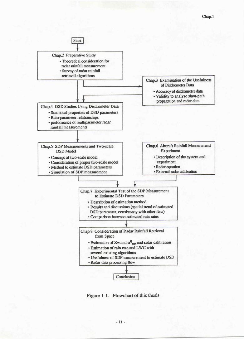
Figure 1-1. Flowchart of this thesis

Chap.l
Figure 1-1 shows a flowchart of this thesis organizndby the following chapters:
Cltnpter 2: Fundamental meteorological and radar quantities are summarized, basic theory of
radar rainfall measurement is outlined, and the radar equations relevant to this study are
described.
Cltapter 3: We consider the DSD measurement by a disdrometer for the study of radar remote
sensing. Followed by an introductory explanation of the disdrometer, consideration is given to
possible errors in disdrometer measuremenl Two experimental data analyses which justify the
use of disdrometer data for the study of radar rainfall measurement are described: (1) an
analysis of slant-path rain attenuation properties, and (2) the external calibration of a Ku-band
FM-CW radar.
Chapter 4.' Based on the experimental validation of the disdrometer data" we perform statistical
analyses of parameters of DSD modeled by gamma and lognormal models, including rain rate
and Z-factor dependences of the DSD parameters, and relations between integral rain
parameters of interest such as Z-R, &-R and k-Z relations as well. In this chapter, the validity
of using the gamma and lognormal models, both three-parameter and two-parameter models, is
tested in terms of the accuracy in rain rate estimation. From the test, we find that the dual-
parameter (DP) rainfall measurement combiningZ and attenuation measurements has suffrcient
accuracy in rain rate estimation.
Clnpter 5: Based on the results obtained in the preceding chapters, we propose a "semi" dual-
parameter (SDP) rainfall measurement combining a Z-factor profile and path-integrated
attenuation for estimating DSD parameters. To do this, we inffoduce the concept of "two-
scale" DSD model and propose some two-scale models adequate for describing short-term (or
small spatial scale) DSD variations. Rain rate profiling accuracy of the SDP measurement is
evaluated through a simulation employing the disdrometer dataset. The result shows that the
SDP measurement has an ability to estimate the rain rate profile reasonably well; 2to 4 times
better than the single-parameter (SP) measurement using a Z-R relation, depending on the
temporal or spatial resolution of the attenuation measurement and depending on the two-scale
model assumed.
Chapter 6.. The DSD estimation methd proposed in Chapter 5 is tested using the data obtained
in the CRL/NASA joint aircraft experiment. For this experiment, the MARS system was
upgraded and installed on the NASA T-39 aircraft. In this chapter, descriptions are given of
the experiment conducted in the fall 1988, the modified MARS system, and the method and
12-
Chap.l
result of external radar calibration.
Chapter 7: Experimental tests of the DSD estimation method are performed using the data
obtained from the T-39 experiment. The methd proposed in Chapter 5 is modified to some
extent so as to allow use of more general IRP relationships and to accommodate the attenuated
Z-factor profile. The validity of estimated DSD parameter is confirmed by means of a
consistency check with the Ka-b and Z-factor profile that is independent of the DSD estimation
process. The test result is found to be very encouraging. It is also suggested that the non-
uniform beam filting and the affenuation due to hydrometeors aloft such as bright band
particles can cause non-negligible errors in the estimated DSD and in the final product (rain
rate and LWC).
Clnpter 8: Based on the results obtained in the preceding chapters together with those
obtained from previous studies, we consider general strategies for processing a spaceborne
radar data to generate accurate and useful rainfall parameters. A discussion is made on the
usefulness of the method proposed in this thesis to improve the overall radar rainfall retrieval.
The proposed DSD estimation method may not always be applicable mainly because of the
effect of non-uniform beam filling and the unavailability of path-integrated attenuation;
however its unique feature to provide the most fundamental rainfall parameter, DSD, will be
very useful to improve rainfall retrieval accuracies for a wide range of rainfall measurements.
13‐
Chap.l
References
(1) Atlas, D. and O.W. Thiele, eds., 1981: Precipitation measurements from space.
Workshop report, NASA/Goddard Space Flight Center, Greenbelt, MD.(2) NASA, 1984: Earth Observing System Working Group Report Vol. I. NASA
TM-86129.(3) Thiele, O.W., ed., 1987: On the requirements for a satellite mission to measure tropical
rainfall. NASA RP-I I83.(4) Simpson, J., R.F. Adler, G.R. North, 1988: A proposed tropical rainfall measuring
mission. Bull. Amer. Meteor. \oc.,69, 278-295.(5) Simpson, J., ed., 1988: A satellite mission to measure tropical rainfall. Report of
the Science Steering Group. NASA/Goddard Space Flight Center.(6) WCRP, 1990: Scientific plan for the TOGA coupled ocean-aunosphere response experi-
ment. WCRP Publ. Ser. No.3 Addendum, Int'l TOGA Project Office, WMO, Geneva.(7) Schiffer, R.A., 1988: Global energy and water cycle experiment (GEWEX). Tropical
Rainfall Measurements, J.S. Theon and N. Fugono, eds. A. Deepak Publ., Hampton,
vA, 2r-25.(8) Wilheit, T.T., 1986: Some comments on passive microwave measurement of rain.
Bull. Amer. Meteor. Soc.,67, L226-1232.(9) Kummerow, C., R.A. Mack, and I.M. Hakkarinen, 1989: A self-consistency approach
to improve microwave rainfall rate estimation from space. I. Appl. Meteorol.,28,
869-884.(10) Atlas, D., ed., 1990: Radar in meteorology. Amer. Meteor. Soc., Boston, 806pp.(11) Meneghini, R. and T. Kozu, 1990: Spaceborne Weather Radar, Artech House,
Norwood, MA, 199pp.(I2) Eckermatr, J., 1975: Meteorological radar facility for the space shuttle. IEEE Nationnl
Telecomm. Conf., New Orleans, IEE Publ.75 CH1015 CSCB, 37-6 - 37-I7.( 13) Skolnik, M.I., 197 4: The application of satellite radar for the detection of precipitation.
NRL Report 2896, October.(14) Okamoto, K., S. Miyazaki, and T. Ishida,1979: Remote sensing of precipitation by a
satellite-borne microwave remote sensor, Acta Astronautica, 6, LO43-1060.(15) , T. Ojima, S. Yoshikado, H. Masuko, H. Inomata, and N. Fugono, 1982:
System design and examination of spaceborne microwave rain-scatterometer.
Acta Astronautic a, 9, 7 l3-7 2L.(16) Goldhirsh, J. and E.J. Walsh, 1982: Rain measurements from space using a modified
Seasat-Type altimeter. IEEE Trars. Antennas and Propag., ArP-30,726-733.(17) Li, F.K., E. Im, W.J. Wilson, and C. Elachi, 1988: On the design issues for a
spaceborne rain mapping radar. Tropical Rainfall Measurements, J.S. Theon and
N. Fugono, eds. A. Deepak Publ., Hampton, VA, 387-393.(18) Okamoto, K. et al., 1988: A feasibility study of the rain radar for tropical rainfall
measuring mission. "I. Comm. Research Lab.,35, 109-208. (This actually consists
of six papers by K. Okamoto, J. Awaka, K. Nakamura, T. Ihara, T. Manabe
and T. Kozu.)
-14-
Chap.l
(19) Goldhirsh, J., 1988: Analysis of algorithms for the retrieval of rain rate profiles from aspaceborne dual-wavelength radar. IEEE Trans. Geosci. and Remote Sens., GE-26,98- 1 14.
(20) Im, E. and F. K. Li, 1989: Tropical rain mapping radar on the Space Station.Proc. /GARSS89, Vancouver, Canada, 1485-L490.
(2I) Marzoug, M., P. Amayenc, J. Tesnrd, and N. Karouche, 1989: Conceptual designof the spaceborne rain radar for the B.E.S.T. project. Preprints,24th Conf. RadarMeteor., Tallahassee, FL, Amer. Meteor. Soc., 597-600.
(22) Okamoto, K., J. Awaka, T. Ihara, K. Nakamura, and T. Kozu, 1989: Conceptual
designs of rain radars in the Tropical Rainfall Measuring Mission and on the JapaneseExperiment Module at the manned Space Station progfirm. Preprints,4th Conf. SatelliteMeteor. and Oceanog., San Diego, CA, Amer. Meteor. Soc., L8-21.
(23) Nakamura, K., K. Okamoto, T. Ihara, J. Awak&, T. Kozu and T. Manabe, 1990:
Conceptual design of rain radar for the Tropical Rainfall Measuring Mission.Int. J. Satellite Communicatiors,8,257 -268.
(24) Okamoto, K., T. Ihara, J. Awaka, T.Kozu, K. Nakamura, and M. Fujita, 1991:Development status of rain radar in the tropical rainfall measuring mission. Preprints,25th Conf. Radar Meteorol., Paris, Amer. Meteor. Soc., 388-391.
(25) Lhermitte, R., 1989: Satellite-borne millimetric wave dopplerradar.URSl Conmis-sion F, Open Symposium,La Londe-Les-Maures, France, Sept. 11-15.
(26) Nathanson, F.8., T.H. Slocumb, S.W. McCandless, and R.K. Crane, 1989: A spacebased radar to measure clouds and rain. Proc.lGARSS '89,Yancouver, Canada, L484.
(27) Im, E. and K. Kellogg, 1990; Spaceborne radar for rain and cloud measurements:A conceptual design. Proc.IGARSS '90, ColLege Park, MD, 425-428.
(28) Atlas, D. and C.W. Ulbrich, 1974: The physical basis for attenuation-rainfallrelationships and the measurement of rainfall parameters by combined attenuationand radar methods, ,I. Res. Atmos.,8,275-298.
(29) _, and R. Meneghini, 1984: The multiparameter remote measurement
of rainfall. Radio Sci., L9,3-22. (This volume is a special issue on multiparirmeter
radar rainfall measurement. Also see a series of papers in this issue.)(30) Stout, G.E. andE. A. Mueller, 1968: Survey of relationships between rainfall rate and
radar reflectivity in the measurement of precipitation. J . Appl. M eteor., 7 , 465-47 4.(31) Atlas, D. and C.W. Ulbrich, 1977: Path- and area-integrated rainfall measurement by
microwave attenuation in the 1-3 cm band, J. Appl. Meteorol., L6, 1322-1331.(32) Eccles, P.J. and E.A. Mueller, 197l: X-band attenuation and liquid water content
estimation by a dual-wavelength radar. J. Appl. Meteor.,10, 1252-1259.(33) Sachidananda, M. and D.S. Zrnic, 1986: Differential propagation phase shift and
rainfall estimation. Radio S ci., 21, 235-247 .(34) Balakrishnan, N. and D.S. 7snic, 1989: Correction of propagation effects at atten-
uating wavelengths in polarimetric radars, Preprints,24th Conf. Rad^ar Meteor.,
Tallahassee, FL, Amer. Meteor. Soc., 287-291.(35) Okamoto, K., S. Yoshikado, H. Masuko, T. Ojima, N. Fugono, 1982: Airborne micro-
wave rain scatterometer/radiometer. Int. J . Remote Sens.,3, 277 -294.
-15-
Chap.l
(36) Fujita, M., K. Okamoto, S.Yoshikado, and K. Nakamura, 1985: Inference of rain rate
prof,rle and path-integrated rain rate by an airborne microwave scatterometer. Radio Sci.
20, 631-642.(37 ) - , ,H .Masuko ,T .o j imaandN.Fugono ,1985 :Quan t i t a t i vemeas -
urements of path-integrated rain rate by an airborne microwave radiometer over ocean.
J . Atmos. Ocean. Tech., 2, 285-292.
(38) Meneghini, R., K. Nakamura, C.W. Ulbrich, and D. Atlas, 1989: Experimental tests of
methods for the measurement of rainfall rate using an airborne dual-wavelength radar.
I. Atmos. and Ocean. Tech.,6, 637-65I.
(39) Meneghini, R. and K. Nakamura, 1988: Some characteristics of the miror image return
inrain.Tropical Rainfall Measurements,J.S. Theon and N. Fugono, eds. A. Deepak
Publ., Hampton, VA, 235-242.(40) Weinman, J.A., R. Meneghini and K. Nakamura, 1989: Comparison of rainfall profiles
retrieved from dual-frequency radar and from combined radar and passive microwave
radiometer. Preprints, 4th Conf. Satellite Meteor. and Oceatng. San Diego, CA,
Amer. Meteor. Soc., 27-30.
(41) Meneghini, R. and K. Nakamura, 1990: Range profiling of the rain rate by an airborne
weather radar. Remote Sens. Environ, 3l, 193-209-
(42) Kozu, T., R. Meneghini, W. C. Boncyk, K. Nakamura, and T. T. Wilheit, 1989:
Airborne radar and radiometer experiment for quantitative remote measurements
of rain, Proc. /GARSS 89, Vancouver, Canada, L499-I502.
(43) Meneghini, R., T. Kozu, H. Kumagai, and W. C. Boncyk, 1990: Analysis of airborne
radar and radiometer rain measurements and their relationship to spaceborne
observations. Proc.lGARSS '90, College Park, MD, 429-432.
(44) Elsberry, R. L., 1989: ONR tropical cyclone motion research initiative: Update on field
experiment planning. Technical Report NPS-63-90-002, Naval Postgraduate School,
Monterey, CA, 64 PP.(45) Kumagai, H., R. Meneghini, and T. Kozu, L991,: Multi-parameter airborne rain radar
experiment in the North Pacific. Preprints,25th Conf. Radar Meteorol., Paris,
Amer. Meteor. Soc., 4m-403.
(46) Ulbrich, C.W. and D. Atlas, L975: The use of radar reflectivity and microwave
attenuation to obtain improved measurement of precipitation, Preprints, I6th Conf-
Radar Meteorol., Houston, TX, Amer. Meteor. Soc., 496-503.(47) and -,1977: A method for measuring precipitation parameters using radar
reflectivity and optical extinctio n, Ann Telecommun., 32, 4t5-42L -
(48) and -, 1984: Assessment of the contribution of differential polarization to
improved rainfall measurements. Radio Sci., 19,49-57 -
(49) Goldhirsh, J. and I. Katz, 1974: Estimation of raindrop size distribution using multiple
wavelength radar systems. Radio Sci., 9,439-446.
(50) -, 1975: Improved error analysis in estimation of raindrop spectra, rain rate,
and liquid water content using multiple wavelength radars. IEEE Trans. Antennas
Propag., AP-24, 7 l8-72O-
- 1 6 -
Chap.2
b '
CHNPTER 2. PUYSTCAL AND THNONETICAL BASES OF
RADAR RAINFALL MBASUREMBNT
2.1 Rainfall and DSD Parameters
2. 1 . 1 Defi nitions of meteorological parameters
As a preparation for the discussion of radar rainfall measurements, it is helpful to
summarize various radar and meteorological quantities. They include scaffering and absorption
cross sections of a particle, dielectric constant, size distribution of particles, and various
integral rainfall parameters. Table 2-1 lists those parameters and their units used in this thesis-
Although the units used here are very common, it should be noted that they are not unique-
Care should be given to the difference in the units in comparing the results of this thesis to the
results of other papers. More discussions on those parameters follow-
2.1.2 Dielectric constant
Dielectric constant, e, is a fundamental parameter to characteruze the attenuation and
scattering properties of hydrometeors. It is often expressed as a value relative to that of free
space, €0 (= g.g54x LO-L} F/m). The relative dielectric constant t, (= e/eg) is related to the
complex index of refraction, m,by ,rP =e. The q or m of water and ice can be calculated if the
temperature is given. The result by Rayl) is shown in Table 2-2' Fot general nonliquid
hydrometeors which are composed by water, ice and air, however, e, depends also on the
mixing situation of the particle. Several formulae have been proposed to calculate ttre s" of such
mixed hydrometeors, a discussion of which is found in Meneghini and Kozu2)- In this thesis,
the Wiener,s formula3,4) wiil be employed to calculate the E of the bright band particles' In
Appendi x 2-L, an outline of this model to calculaF er is described-
The scattering, absorption and attenuation (or total) cross sections (o5, oa, and 01,
respectivety) of a single hydrometeor are dependent on the dielectric constant of a particle'
particle size and shape, and the wavelength and polarization of the incident wave' Hydro-
meteors can be approximated as spherical or deformed (oblate spheroid or Pruppacher-Pitter5)
form) drop models. In most non-polarimetric radar measurements, the assumption of spherical
shape may be. sufficient 6). The cross sections of a spherical particle can be calculated with
-17
Chap.2
Quantity Symbol Definition Unit
Imaginary part of m m1
Dielectric factor K
Dielectric factor of water Kw
Mass density
Drop diameter
Scattering cross section
Falling velocity
nth moment of DSD
Radar reflectivity
Radar rcflectivity factor
Effective radar reflecl factor
Rainfall rate
Attenuation coefficient
Liquid water content
Optical extinction
2.99792x10⁸m = f n R - i m t
(*2 - L)te* +2)
O t = O s * O x
fJDaN(D) dDI
Jou@W@) dDt -JDoN(D) dD
I
1 g I 814n -stKd-2 lou(D)N(D) dD
f0.0006nJv@)DtN(D a
I4343Jo(D)N(D) dD
pttt6xroalozu1U dD
nt1xLo-3[nzug dD
ft.cm
mp
pDO5
Hz
m
m/sec_ * l
gl" 3
rnm
m2
m2
n2
m2
*o-r1n3
m/sec
66nftn3
m-1
prn67p3
pp6113
mm/hour
dB/rrn
d^3
6n-l
Absorption cross section <l3
Total cross section og
Backscattering cross section 06
Drop size distribution (DSD) N(D)
v(D)
Mn
Tl
Z
Ze
R
k
w
E
'tl "rn' is also used for a parameter of gamma dropsize distribution'
18‐
Chap.2
Table 2-2. Complex refractive indices of water and ice for several radar fiequencies.
Frequency TempmmE ″ 沢 “ J |バ12
5。33 GIIz
10.∞ GI・L
13.80(〕H2
17.25GL
24.15G比
34.50 GI・Iz
30°C
20°C
10°C
O°C
O°C(iCep
30°C
20。C10°C
O°C
O°C(iC0
30°C
20°C
10°C
O°C
O°C(iC0
30°C
20°C
10°C
O°C
O°C(iC0
30°C
20°C
10°C
O°C
O°C(iC0
30°C
20°C
10°C
O°C
O°C(iC0
8.576
8.650
8.625
8.423
1.782
8.185
8.032
7.682
7。087
1.781
7.786
7.465
6。938
6.221
1.781
7.405
6.972
6.361
5。621
1.781
6.684
6。133
5.482
4.791
1.780
5.805
5.233
4.637
4.057
0.1780
0.962
1.265
1 . 6 6 8
2.175
。003636
1.649
2.059
2.507
2.907
0.002324
2.066
2.462
2.815
3。034
.001848
2.341
2.680
2.922
3.002
.001576
2 . 6 6 1
2.851
2.902
2.802
.∞1241
2.799
2.803
2.685
2.464
.0009626
0。9249
0.9279
0。9307
0。9332
0.1767
0.9241
0。9267
0.9287
0。9298
0.1764
0.9232
0.9251
0。9261
0。9255
0。17“
0.9221
0.9234
0.9232
0.9205
0.1764
0.9193
0.9187
0.9154
0.9076
0.1760
0。9137
0。9093
0.8998
0.8819
0.1760
the Mie theory. The description of the Mie theory can be found in a number of text books (e.g.
StrattonT)). Scattering coefficients of deformed drops have been calculated by employing
several techniques such as point-matching and least-square fitting methods, spheroidal
function expansions methods, and T-matrix methods 89). Since the symmetry axes of falling
raindrops are aligned along the vertical direction on average, the spherical particle model may
be used for the study of down-looking radar measurement. This hypothesis will be evaluated
later in this section.
According to the Mie theory, the scattering, absorption and total cross sections, os, ox,
and o1 are given by
19-

os=λ2/(2π)通′(2″+1)(αメ2+bJ2)
σt=―λ7/(2π)Σ(2κ+1)Re[α″+b″]■ ■1
% = 6 t― Os
Chap.2
(2。1)
(2.2)
(2。3)
(2.4)
(2.5)
(2.6)
(2.7)
(2◆8)
(2.9)
where 2u is the wavelength in background medium. The expansion coefficients an and bn arl-
called Mie coefficients, and are expressed in terms of spherical Bessel functions and Hankel
functions of the second kind with arguments 26 (= 2nrlL, r being the radius of the particle) and
the relative complex dielectric constant, e1. The anandb,Trepresent the scattered frelds arising
from the induced magnetic dipoles, quadrupoles, etc. and electric dipoles, quadrupoles, etc.,
respectively. Similarly, the Mie backscattering cross section, 06, is given by
6b=22/(4π)IΣ(-1)″(2“+1)(α.‐b″)p■ ‐'
- Raylei gh approximatio n
Much simplification is possible in the above expressions of os, oa, 01 and o6, when the
particle size is much smaller than the wavelength 1., which is known as Rayleigh
approximation. With this approximation, os, Oa, Gt and o6 ire expressed as
widl
os=2/3(π5A4)D61厠 2
6a=鰊 2ADD31m[―珂
。b=(π5/24)D61厠2
κ=(Cr-1ソ (Cr+2)
【″=(Cr-1)/Cr+2), with er fOr water.
where D (= 2r) is the diameter of the particle. A criterion of the diameter range where the
Rayleigh approximation is valid is d-e4l < 0.5 l0). Eqs. (2.5) through (2.8) state that os and o6
are proportional to D6, while o2 is proportional to D3 in the Rayleigh region. Because of the
difference between the panicle size dependences of os and oa, os is generally much greater
than os (i.e., or = o) when D << 1,. The dielectric factor, K, for water (hereafter Kn) is later
used to define the effective radar reflectivity, Ze:
-20-
(2.10)

Atlas‐Ulbrich(Eq
Gunn-Kinzer &
Uplinger (Eq.2.11)
Chap.2
1.1979-
Apr.30,19801 .
1.4
1.
RAU = 1-001 Rcx - 0'029
.5 1 1.5 2
L o g 1 0 o f r a i n r a t e , w i t h v G K ( R G K )
Figure 2-1 Terminal fall velocity of raindrops using different equation5, ild comparison of rain ratescalculated from ground-measued DSDs using terminal velocities vUp(D) ndvAg{D).
2.1.4 Terminal fall velocity
Rain rate is among the rain parameters most often required from meteorological,
hydrological and cloud physics studies. Since the rain rate is the downward flux of water, it is
essential to know the terminal fall velocity of hydrometeors. Gunn and Kinzerll) data have
widely been used as the raindrop terminal velocity on the ground- The height or air densiry
dependence of the terminal velocity can be simply expressed by the factor (p(0)/p(z))o'4, PQ)
being the air density ar heighr z, mulriplied ro the Gunn-Kinzer velocity, vcdD), which was
given by Foote and du Toit t2). It is sometimes convenient to approximate the VGK(D) by an
analytic function. In this thesis, we use the following two functions:
( 2 . 1 1 )
(2.12)
(っく∝) っく>〓一一〓.Φ一”」C一“』一0。一〇0コ
なΦ契E)む一opΦ>雨
・⊆E」Φト
2
1 . 8May
2 4 6
Drop diameter(mm)
ソυンCD)=4.854 D exP(-0。195D)
VAυC))=3.778 DO・67
where the velocity is in m/sec and the drop diameter is in millimeters. A comparison of vGK,
vg, andv4y is shown in Figure 2-1. The former, proposed by Uplingerl3), gives an
excellent fit over the entire drop diameter range up to about 5.5 mm and will be used to
calculate the rain rate from measured and theoretical DSDs. The latter, proposed by Atlas and
Utbrichla), gives less accurate fit than the former; however, we will employ it in making
approximate comparative analyses between rain rate and other rain parameters, since with
vau(D)rain rate is expressed as a quantity proportional to the 3.67th moment of DSD' In
order to evaluate the validity of vN/D), rain rates are calculated from DSDs measured on the
groundusing vau(D) and v56(D). The result, also shown in Figure 2-1, indicates thatvlu(D)
is sufficient for the purpose mentioned above-
-21
Chap.2
2.1.5 Drop size distribution (DSD)
a. Importance of knowledge of DSD
Size distribution of precipitation particles (DSD) is a fundamental precipitation
parameter by which all integral rain parameters (IRPs, see section 2.L.6) and relationships
among them are characteiznd. Because the direct radar measurable, radar reflectivity, is
approximately proportional to the 6th moment of DSD and different from the other IRPs of
interest, the knowledge of DSD is essential to make an accurate radar estimation of IRPs. It is
known that DSD is highly variabler5-18). Examples of such DSD variation are shown in Figure
2-2, which were measured on the ground by a disdrometer (see Chapter 3 for the details). It
changes from time-to-time and from one rain event to another. Although there have been
numerous studies to understand, to parameterize and to estimate DSD, large uncertainties
remain in temporal and spatial DSD variabilities and their dependence on rainfall type and
climatological regimes.
b. DSD models
Although natural DSDs are highly variable, thrce-parurmeter models such as g^mma and
lognormal models are known to fit the natural DSDs well. Two-parameter models are less
flexible but still provide god fitting to the natural DSD's in a limited domain. They are
considered to provide a sufficient accuracy to relate rainfall parameters of practically interest
such as radar reflectivity, rain rate, LWC and microwave attenuationl8,l9). The reason is that
alt of those rain parameters are mainly determined by distributions at intermediate to large drop
diameters and therefore variations in distributions at small drops can be neglected.
The DSD model most frequently used to date is the gamma disribution:
ⅣCD)=NO D″ exP(―AD)=Ⅳ r型今手11言:‖「
eXP(―AD) ( 2 。1 3 )
where [Ng,m,A] or [Nr, m,Ll are parameters of the gamma model. Although Nr is the zeroth
moment of the DSD modeled as gamma, we treat it also as a DSD parameter that can be used in
place of Ng 20). The parameter rn is often fixed for simplicity and for making it possible to
estimate DSD from dual-parameter radar measurements. The exponential distribution is a
special case (m - 0) of the gamma distribution and expressed as
N(D) - N0 exP(-AD) = Nr A exP(-AD)
where [NO, A] or [Nf, A] are parameters of the exponential model.
‐22-
(2.14)
Chap.2
Another DSD model that is sometimes employed is the lognormal distribution
N(D):+exp(- %) (z.rs)
aDl2n
where [NnF,o] are parameters of the lognormal model. Similar to the m parameter of the
gamma model, the parameter o is often 6*"dl72l).
The other problenl in the DSI)modeling is to characterize the
varladon in DSDo For exalnple,dlc Marshall―Palmer erゾD DSD model
Ⅳの )=No exp(…AD),with No=8000 and A=4.lR-0・21
spatial or temporal
(2.16)
assumes that Ng is constant and A is related to rain rate R by a negative power law. Similar
DSD models were proposed by Joss et al.ls):
NO=1400 and A=3.OR-0・ 21
NO=7000 and A=4.lR-0。 21
NO=30000 and A=5。 7R-0・21
Joss-Thunderstorm (J-T)
Joss-widespread (J-SD
Joss-Drizzle (J-D).
It has been reported that the MP model fits well to natural DSDs if a large number of DSDs are
averaged in spite of the large fluctuation in short term DSDs 18'23). Since theZ factor or rain
rate dependences of the DSD par:rmeters are closely related to the relationships among various
rain parameters, it is important to investigate such DSD fluctuation properties. In comparison
to the modeling of individual DSD, the number of studies concerning to this problem is
relatively small. Although there are many papers concerning the relationships among rainfall
parameters (especially Z-R relation) 2425) and although it is well known that such IRP
relations are formed as a result of DSD variation, relatively limited number of papers give a
quantitative discussion on the relation bemreen "DSD variation" and the "relation between two
rainfall parameters" 26,27). We will consider this problem in detail and connect to the
estimation of DSD parameters using a practically feasibte radar system from space-
…23‐

Chap.2
(?ETEE)Lo一“饉〓00coO
ΦEコ一o>α90b
〇一ooコ
(a)September 30.1979
1 2 3 4
(b)Ck式 Ober 16,1979
2 3 4
08:46 9′307797.8 rnmJh
NO=93x103
16:36 10′16779
5.7 mmlh
N O = 0 . 2 1 x 1 0 3
1 2 ■ ■ 5
08:49 9r30J796.6 mmJhN O‐5 1 x 1 0 3
o 1 2 3 4 5
DЮ p Diarneter(mm)
5
(9ETEE)〓o一冨」〓ΦocoO
ΦEコ一o>Q20ち
O,ooコ
1 2 3 4 5
o 1 2 3 X4 5
Drop Diameter(mm)
Figve2-L Exarnples of nanrral DSD measured by a disdrometer (see Chap.3). Solid line
represents an exponential model fit using a moment method-
08:04 9′30r796.7 mmJhN 0 8 6 7 x 1 0 3
o 1 2 3 4 5
1 6 : 2 1 1 0 r 1 6 r 7 9 .2 9 2 m m J h
N O = 2 . l x 1 0 3
16」2 10rlげη27.8『nmJh
NO=2.Ox103
o 1 2 3 ■ 5
1 6 : 3 3 1 0 r lげ刀
16.3 nlmrh
NO=0.63x10³
1 2 3 4 S
17:59 10rl"9
5 2 m m r h
NO=0.87x10³
18:02 10r16r795 4 m m J h
NO=1.2x10³
o 1 2 3 4 . 5o 1 2 3 4 5
- 2 4 ‐
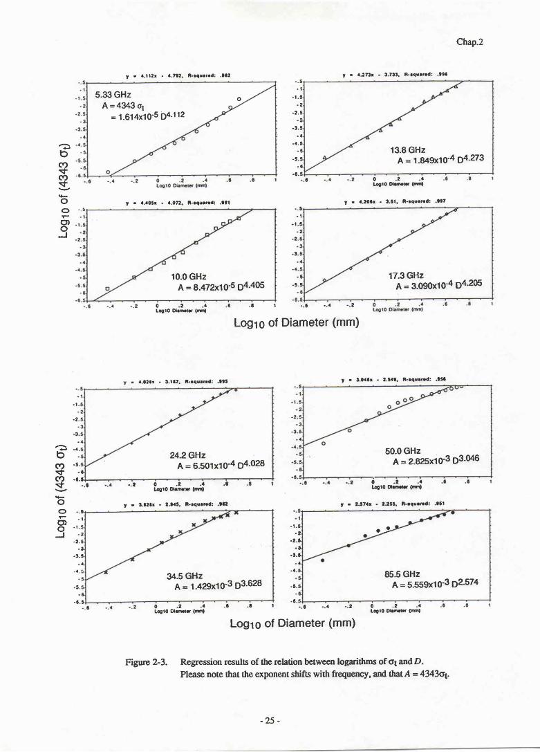
v ● 4.112■ ・ 4.792. R・ 3qu●『ed: .002
5。33 GHz 。
A = 4 3 4 3 σt=1.614x10‐ 5D4。112
Chap.2
I . 1.273r - !.7tt. F-.qs.t.d: .996
13.8 GHz
A=1.849x10‐ 4D4_273
0 .2 .4‐ 10● “腱te c― D
.8 1 ・.6 ・ 。4 ・ .2
Logro of Diameter (mm)
一.
.
L
.
2.
.
3.
.
4.
.
5.
.
●.
つo
∞寸∞寸)一〇orOOJ
・2 .
o3.
・5 。
0 .2 .4Lo010 01omet“c― D
`.0208 ・ 3.107. R‐ oquared: .005
0 .2 .4L(η10●錮腱t“C―D
つo
∞寸∞寸)一〇or00J
・0。50 ・.2 0 。 2 .4 .●
町 10● 躙腱t“1鷹■
v ・ 3.620■ ‐ 2.“ 5, R‐oqoo7od: .982 t - 2.371t - 2155, F-rqu.r.d: .l5l
● タ
85.5 GHz
A=5.559x10‐ 3D2.5745
・6.5
・2
‐2.6
・9。|
6
Los;o o,
oヽ %4 、 2 路 1。面乱ぼ`高
Diameter(mm)
Fignre 2-3. Regression resuls of the relation between logarithms of o1 andD.
Please note that the exponent shifs with frequency, and thatA = 4343ot
y r '|.'r0ir . 4.072. R..rlu.t d: .eet
10.O GHz
A=8.472x10‐ 5D4.405
t . a.2oCr . t.tl. R'.qut?.d: .ect
3
・5
‐5.5
17.3 GHz
A = 3 . 0 9 0 X 1 0‐4 D 4 . 2 0 5
24.2 GHz
A = 6 . 5 0 1 x 1 0‐4 D 4 . 0 2 8
y . 3.0acr - 2.!ta9. R-rqur..d: .tsa
o .2 .4嗜 1001-tr c― D
50.O GHz
A=2.825x10‐3b3.046
34.5 GHz
A = 1 . 4 2 9 x 1 0‐3 D 3 . 6 2 8
|
-25‐
Chap.2
2.1.6 Inteeral rainfall parameter (IRP)
As shown in Table 2-1, most of the rain parameters of scientists' and communications
engineers' interest are defined as the integral of the product of a "kernel", K(D), and DSD,
Such quantities are called "integral rainfall parameten (tRP). A major task of radar rainfall
measurement is to estimate IRPs of interest from IRPs directly obtained from radar
measurements. (Note that the IRP can be defined regardless of particle phase even though we
call it Integral "Rain" Parameter.) The IRPs most important for the radar rainfall measurement
include radar reflectivity factor Z, effecive radar reflectivity factor Ze, attenuation coefficient
k, rain rate R, and liquid water content IV, which are defined in Table 2-1.
For making studies on the IRPs and DSD, it is convenient to approximate the IRPs by
ttre xth moment of DSD, M*, which is defined by
N(D), over the drop diameter, D:€f
IRP = J *tPl N(D) dD.0
IM*: J o* N(D) dD
0
and expressed as the following equations for gamma and lognormal DSD models
M*s^,a=Noffi_Nrffiii
″X10gnOrrnd=崎exp(Xμ+告X2′)
(2.17)
( 2 。1 8 )
(2.19→
(2.19b)
where x may be non-integer. In Table 2-3, such moment approximations are summarized. In
the case of the moment approximation of attenuation coefficient, the order of the moment, .r,
depends on frequency. Around 10 GHz, x takes the maximum value of about 4.5. With
decreasing or increasing the frequency, x decreases due to the increasing contribution of o3 to
01 &t lower frequency and due to the increasing Mie scattering effect at higher frequency.
Figure 2-3 shows regression results of the relation between logarithms of os and D at several
frequencies, from which the x value is obtained. The x value close to 3.67 at35 GHz indicates
that the attenuation measurement at around this frequency should provide an accurate rain rate
estimate.
-26‐
Chap.2
Table 2-3. Moment approximation of typical IRPs (IRP = C Mil.
Integral rain parameter n C Unit
Radar reaccd宙ty factott Z 6 1
Effective radar reflect.factor,Z` -6 1
mm6/m3
mm6/m3
mm/hOlr
dB/km
典3
h m - 1
Rainfall rate, R
Attenuation coefficient, k
Liquid water content, W
Optical extinction, E
* I S." Eq.2.l l. "2 o(o) = CkDv, where v = 3 - 4.5 (dependent on frequency).
2.1.7 Melting layer Gright band)
The information of thermodynamic phase is essential for accurate rainfall retrievals. The
melting layer, at which frozen hydrometeors melt into rain, is very clearly seen by radar in
stratiform rain. Because the melting process causes a clear enhancement in radar reflectivity for
frequencies approximately less than 2O GHz,the melting layer is often calted "bright band"25)-
For convective storms, it is generally difficult to identify where the melting occurs because of
the strong updrafts in the cloud unless multi-firequency or polarimetric radars are employed- In
this sense, the stratiform rain is easier to be modeled than the convective storrns. Examples of
radar reflectiviry profile for stratiform and convective storrn arc illustrated in Figure 2-4.
During a stationary stratiform rain, it may be reasonable to assume that the water flux
(i.e., rain rate) is constant from the top to the bottom of a stonn. This assumption may be
extended up to the bright band if water vapor condensation mainly occurs upper the bright
band and if evaporation affects little to the flux-
Even with this constraint, there are many parameters charactenzing the bright band in
terrns of scattering and attenuation properties. Those include drop size distribution, falling
velocity, particle shape, orientation and dielectric constant. A number of bright band models
have been proposed to 6u1s28-32). Although the shape of melting particle may be highly
irregular, it is almost impossible to know the shape of each particle, shape distribution and
orientation precisely. As a first approximation, therefore, spherical or spheroidal particle model
has been used to calculate the scattering properties-
3.67 6x3◆ 78πx10‐4
3~4。5 4343 Ck
3 pπ ノ6x10‐3
2 π 2x10‐3
1
2
‐27‐
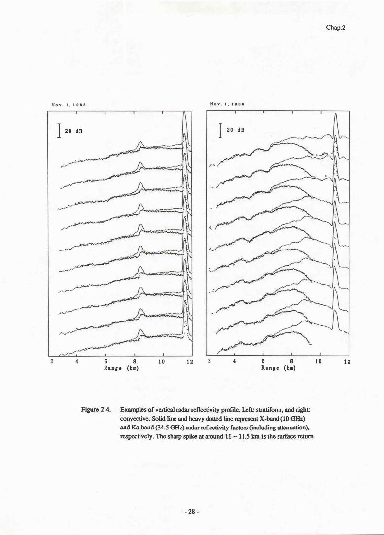
Chap.2
JrodB
5 8Range ( tn )
6R a n g e
28
■
Figure 24. Examples of vertical radar reflectivity profile. I-efr stratiform, and righc
convective. Solid lirp and trcavy doued line represent X-band (10 GIIZ)
and Ka-band (34.5 GIIZ) radar reflectivity facors (ncluding auenuation),
respectively. The sharp spike at around I I - I1.5 km is the surface return.
-28 -

Chap.2
Although there are two types of bright band par-ticle model (concentric two-layer sphere
and composite dielectrics models), no conclusion has been obtained which is better. tn this
thesis, we adopt the latter model together with a NoncoalescenceA.lonbreakup (N/N) model to
estimate the DSD in the bright band. These models have been studied by Awaka et a1.30). They
compared ttre NA{ model with a modified Nishitsuji (M-I.D model a) in terrns of the agreement
with measured C-band Z factor profiles. Their conclusion is that the M-N model, which is
considered to take physical processes in the bright band into account empirically, appears to be
superior to the N/N model in the upper portion of the bright band. For the lower region of the
bright band, however, the difference between the two models are small and the both models
show good agreement with the measured profile. Since the major issue on the bright band in
this thesis is to estimate the affenuation caused by the bright band that would occur at the lower
portion of the bright band, for simplicity, we adopt the N/N model for the retrieval of bright
band together with a composite dielectrics model for individual particle. The outline of the
composite dielectrics model and the N/N model is outlined in Appendix 2-1.
2.1.8 Storm structure
In order to develop rainfall retrieval algorithms using a limited number of remote
sensing data, the use of proper storrn structure model is required and it should be as simple as
possible while keeping a reasonable representation of microphysical phenomena. For example,
vertical storrn models used for passive microwave rainfall rerieval to date consist of one
uniform rain region plus one or several ice and ice+rain mixing layers. Melting layer or bright
band that is a distinct radar precipitation signature has been omitted in the passive rainfall
sensing to simplify radiative transfer computations 33'34).
The radar, which has a capability of profiling, does not require such a simplification for
vertical structure model. Yet, the knowtedge of the storrn structure is required to understand
the radar signatures and estimate various precipitation parameters adequately, and to evaluate
the effect of non-uniform beam filling on the accuracy of the algorithm. The modeling of
strariform type rain is fairly easy because of the existence of clear bright band; rainfall is
horizontally uniform and understanding the vertical stnrcture would suffice for most purposes.
On the other hand, convective type storrns are more difficult to model because the strong
updraft causes the mixing of different hydrometeors such as supercooled water drop, ice and
melting particles, and because the horizontal variability in rainfall is much larger than that of
the stratiform rain. In Chap ter 7 , we will use simplified vertical rain structure models to
-29-
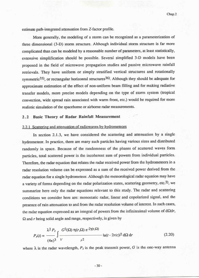
Chap.2
estimate path-integrated attenuation from Z-factor profile.
More generally, the modeling of a storrn can be recognized as a parameterization of
three dimensional (3-D) storrn structure. Although individual storrn structure is far more
complicated than can be modeled by a reasonable number of parameters, at least statistically,
extensive simplification should be possible. Several simplified 3-D models have been
proposed in the field of microwave propagation studies and passive microwave rainfall
retrievals. They have uniform or simply stratified vertical structures and rotationally
symmetric35), or rectangular horizontal structures36). Although they should be adequate for
approximate estimation of the effect of non-uniform beam filling and for making radiative
transfer models, more precise models depending on the type of storm system (tropical
convection, wide spread rain associated with wtum front, etc.) would be required for more
realistic simulation of the spaceborne or airborne radar measurements.
2.2 Basic Theory of Radar Rainfall Measurement
2.2.1 Scattering and attenuation of radiowaves by hydrometeors
In section 2.1.3, we have considered the scattering and attenuation by a single
hydrometeor. In practice, there are many such particles having various sizes and distributed
randomly in space. Because of the randomness of the phases of scattered waves form
particles, total scattered power is the incoherent sum of powers from individual particles.
Therefore, the radar equation that relates the radar received power from the hydrometeors in a
radar resolution volume can be expressed as a sum of the received power derived from the
radar equation for a single hydrometeor. Although the meteorological radar equation may have
a variety of forms depending on the radar polarization states, scattering geometry, etc.2), we
summari ze here only the radar equations relevant to this study. The radar and scattering
conditions we consider here are: monostatic radar, linear and copolarized signal, and the
presence of rain attenuation to and from the radar resolution volume of interesl In such cases,
the radar equation expressed as an integral of powers from the infinitesimal volume of dCldr,
C) and r being solid angle and range, respectively, is given by
G2(Ω)η(r,Ω)C‐2Kr,Ω)
lu(t - 2rl)12 dCt dr (2.20)
ls the one―way antennais the peak ffansmit power, G
Pr(の=里 ∫(4π)3 r2
為where l" is the radar wavelength,
-30‐

Chap.2
gain, u(r) is the complex envelope of the transmitted pulse normalized to have the peak
amplitude of unity. Tl and y are radar reflectivity and optical depth of rain, respectively, which
are given by
η= (2。21)
Kr)=0.1 (2.22)
where the definition of the quantities used in Eqs.(2.21) and (2.22) are given in Table 2-1.
The following approximations hold for most cases: (1) Most of the transmitted energy is
concentrated in a narrow main beam so that the radar reflectivity and rain attenuation are
independent of angular variations; (2) Antenna gain pattern is given by a two-dimensional
Gaussian function and sidelobe contribution to the received power can be neglected. With
these approximations, Eq.2.20 becomes
長bの)Ⅳの)dD=π51獅12λ4盈0
lnlolil(∫ )ds
O
r
Zc exp[-0.2 1nlC)∫た(s)ds]=0
(2.23)
with π3Pr Go2 0B2“
(2.24)
lO24ln2L2
where Go is the peak antenna gain, 0g is the half-power antenna beamwidth, c is the speed of
light, and t is the transmitted pulse width. For convenience, "apparent" or "measured"
effective radar reflectivity factor,Ztlt, is also introduced.Zmis recogniznd as an estimate of Ze
using a radar equation neglecting rain attenuation. SinceZm can be estimated with the radar
system parameters only, it is convenient to begin the rain parameter estimation with this
quantiry and we will frequently use it in this thesis.
- Dffirence inZe values between spherical and deformed drop models
Since the present study concerns the radar observation using near-nadir incidence angles
at which there is linle polarization difference in scattering propenies, it may be sufficient to use
the spherical model. The Mie theory may then be used to calculate all scattering and attenuation
cross sections, which makes the calculation much easier than that for the deformed drop
models. However, it may be required to check the difference between the spherical and
C =
-31-
Chap.2
deformed drops having the same volume, because the effective diameter of the deformed dtop
is larger than that of the spherical drop when the drop is seen down or upward. For this
purpose, comparisons are made for Ze factors calculated from the spherical and deformed
(Pruppacher-Pitter) drops. For the calculation of the deformed drop case, we use the result
from Oguchi's point-matching-and-least-squarcs method3T), (M. Satake, private communica-
tion). Since Ze is approximately proportional to the 6th moment and put the largest weight on
the large drops among the IRPs of interest, it should be sufficient to check the difference in Ze.
The result is shown in Figure 2-5 for l0 GHz and 35 GHz which are used in the airborne
radar system we will employ later in this thesis. It is found that the differences in Ze factors (in
dB unit) increase with rain rate to some extent depending on frequency and DSD. It appears,
however, that the difference is minor in comparison to the large variation in DSD that causes
large fluctuation in Ze-R and k-Ze relations, and that it can approximately be treated as a
constant bias of several tenth of decibels.
Based on the above consideration, we use the spherical drop model both for raindrop
and bright band particles.
. 6 . 8 1 1 . 2 1 . 4
logrs of Rain rate (mm/h)
Figure 2-5 Difference in 7z frctors of the spherical drop model and the deformed drop model
at l0 GHz and 35.5 GHz assuming the two-parameter gamma DSD models
given in Table 4-2, with m = Oand m = 6 .
(■.LON一\一”。tΦ〓Q∽ONじ〇一〇〇一0,
1。81.6
35.5 GHz
10。O GHz
A f i I = 6
O O f f i : 0
- 3 2 -

Chap.2
2.2.2 Estimation of mean received power and radar rcflectivitlr
Since the hydrometeors in a radar resolution volume are randomly distributed and
fluctuating rando-ly, the radar precipitation return shows large fading due to the interference
among return signals from each scatterer. The quantity that should be obtained by a radar
precipitation measurement is the radar received power, Pr, that is defined by the radar equation
described above; the sum of received powers from individual scatterers. The most common
method to estimate P, is to use the average of the fluctuating instantaneous received signal
level. For the estimation, some assumptions are usually employed: (1) The fluctuating return
signal is ergodic so that both ensemble and time averaging can be used; and (2) many small
scatterers arc randomly distributed in a resolution volume which is much larger in size than the
radar wavelength, so that the phase of the composite return signal is uniformly distributed over
O to 2n and the amplitude is Rayleigh distributed-
It follows from the assumption (2) that the instantaneous return power, P, is
exponentialty distributed; i.e. the probability density function (pd| of P, p(P), is given by
p(P)=Pr‐l exp(‐P/Pr). (2.2s)
The exponential pdf has the standard deviation equal to the mean value Prand therefore the
estimation of Pr from a single measurement suffers from a large error. In order to reduce the
estimation error, many samples statistically independent should be averaged. The averaging is
made after the detection of IF signal. The pdf of the averaged video signal depends on the type
of detection. For a square-law detection, the pdf of the average of N independent video
signals, pN(€), can be written in the form of the 26-squared distribution of 2N degrees of
freedom38):
,yN qN-l N
exp( - NE/Pr ) , q -N- l IP ii = I
pNC)= (2.26)PrN W -l)l
so that the expectation (EC)) and variance (Var(')) of ( are P, and P?/tt,respectively.
For the logarithmic detection that is frequently employed to increase the dynamic range,
the pdf of the average of loglg (P/Pr), pllr((), is approximated by391
- 3 3 -
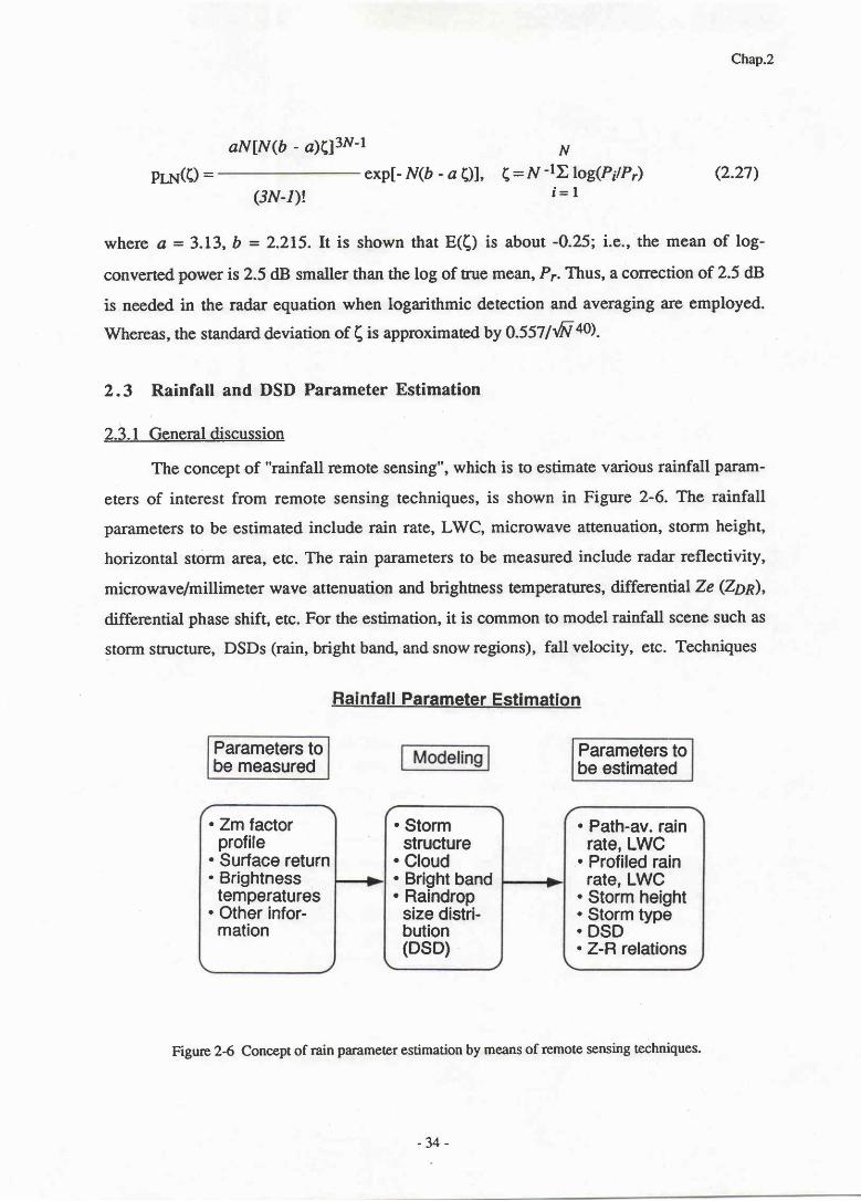
Chap.2
aN[N(b - 4X]3N-l N
( = N -rElog(P;lPr)
f = IpLN(ζ)= eXp[―N(b―α01, (2.27)
(3N-/)!
where a = 3.L3, b - 2.215. It is shown that E(() is about -0.25i i.o., the mean of log-
converted power is 2.5 dB smaller than the log of tnre mean, Pr. Thus, a correction of 2.5 dB
is needed in the radar equation when logarithmic detection and averaging are employed.
Whereas, the standard deviation of ( is approximated by 0.557\Vff+Ol.
2.3 Rainfall and DSD Parameter Estimation
2.3.1 General discussion
The concept of "rainfall remote sensing", which is to estimate various rainfall param-
eters of interest from remote sensing techniques, is shown in Figure 2-6. The rainfall
parameters to be estimated include rain rate, LWC, microwave attenuation, storrn height,
horizontal storm area, etc. The rain parameters to be measured include radar reflectivity,
microwave/millimeter wave attenuation and brightness temperatures, differenial Ze (Zon),
differential phase shift, etc. For the estimation, it is common to model rainfall scene such as
storrn structure, DSDs (rain, bright ban4 and snow regions), fall velocity, etc. Techniques
Rainfall Parameter Estimation
Parameters tobe measured
Parameters tobe estimated
Figure 2-6 Concept of rain parameter estimation by means of remote sensing techniques.
-34 -
. Zm factorprofile
. Surface return
. Brightnesstemperatures
. Other infor-mation
. Stormstructure
. Cloud
. Bright band
. Raindropsize distri-bution(DSD)
. Path-av. rainrate, LWC
. Profiled rainrate, LWC
. Storm height
. Storm type
. DSD
. Z-R relations

Chap.2
to be employed are closely related to the requirements such as accuracy and spatiaVtemporal
resolutions. For example, if only rainfall or rain rate statistics for a long period (e.g. a month)
or a wide area are required, statistical properties of rainfall can be utilized to estimation
techniques, which should reduce the difficulty in comparison to the estimation of instantaneous
rain rate profrls4 l'42).
As can be seen from Table 1-2, there is a variety of requirements ranging from one
month and 500 km to about a half an hour and several kilometers. In the case of radar
measurements, it is ttre most basic problem to estimate rainfall paftlmeters in a radar resolution
volume which is approximately several hundrcd meters in range and several kilometers in
horizontal dimension. Development of rainfall parameter estimation techniques with fine
temporaVspatial resolutions is important" because the fine resolution rainfall mapping is a basis
to understand large scale rainfall statisticat properties and is essential for various climatologicat
studies, short range weather forecast, and other cloud/rainfall microphysics. In this thesis,
therefore, emphasis is given to the rainfall parameter estimation with high spatiaVtemporal
resolution.
In the following, rainfall and DSD parameter estimation methods are classified in terms
of the number of measurable rain parameters; single, dual and multi-parameter measurements.
Methods to estimate rain rate by spaceborne radar measurements are also reviewed briefly and
classified in this manner.
2.3.2 Single-parameter (SP) measurements
The conventional way to estimate rain rate and LWC, W, is to use empirical
relationships between Z andR and between Z and 17. Such methods are regarded as Single-
Parameter (SP) measurements. In general, the SP measurement can be defined as estimating
IRPs from a "single" IRP. Because of the difference in the weighting functions, the
relationships between Z and other IRPs depend on DSD (see Figure 2-7). From the DSD
parameter estimation point of view, the SP measurement has an ability to estimate only one
DSD parameter. since at least two parameters are required to express reasonably the natural
DSD, it is anticipated that the SP measurement has a limited capability to estimate IRPs. If one
can measure an IRP that has a kernel close to that of the IRPs to be estimated, estimating the
two DSD parameters is not so essential to obtain sufficient accuracy; e.g. estimating rain rate
from Ka-band (= 35 GHz) attenuationl4). However, such measurement can not always be
accomplished.
- 3 5 -
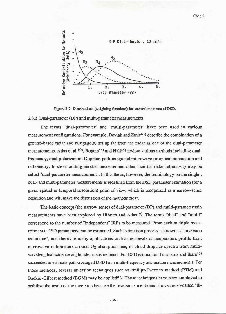
Chap.2
Drop Dlameter (rrn)
Figure 2-7 Distributions (weighting functions) for several moments of DSD.
2. 3. 3 Dual-parameter (DP) and multi-parameter measurements
The terrns "dual-parameter" and "multi-parameter" have been used in various
measurement configurations. For example, Doviak and Zrnica3) describe the combination of a
ground-based radar and raingage(s) set up far from the radar as one of the dual-parameter
measurements. Atlas et al.l9), Rogers44) and Halta5) review various methods including dual-
frequency, dual-polarization, Doppler, path-integrated microwave or optical attenuation and
radiomeury. In short, adding another measurement other than the radar reflectivity may be
called "dual-parameter measurement". In this thesis, however, the terminology on the single-,
dual- and multi-paftlmeter measurements is redefined from the DSD parameter estimation (for a
given spatial or temporal resolution) point of view, which is recognized as a narrow-sense
definition and will make the discussion of the methods clear.
The basic concept (the narrow sense) of dual-parameter (DP) and multi-parameter rain
measurements have been explored by Ulbrich and Atlasl9). The terrns "dual" and "multi"
correspond to the number of "independent" IRPs to be measured. From such multiple meas-
urements, DSD parameters can be estimated. Such estimation process is known as "inversion
technique", and there are many applications such as retrievals of temperature profile from
microwave radiometers around 02 absorption line, of cloud dropsize spectra from multi-
wavelengthsflncidence angle lider measurements. For DSD estimation, Furuhama and lharaa6)
succeeded to estimate path-averaged DSD from multi-frequency attenuation measurements. For
those methods, several inversion techniques such as Phillips-Twomey method (PTM) and
Backus-Gitbert method (BGM) may be appliedaT. Those techniques have been employed to
stabilize the result of the inversion because the inversions mentioned above are so-called "ill-
(一
一Eつ 、LoL一
}OLく
)
∽やCOE
O〓 0一 CO
r一コ0
}L一C00 0>
一↓0
けo∝
Distributlon,
- 3 6 -

Chap.2
posed" problem. Differences between the above applications and the multi-parameter
measurements using the radar are that the latter is not necessarily "ill-posed", and that the
number of measurable independent rain parameters is very limited. Because of these facts in
the dual- and multi-parameter radar measurements, the usual way to make the inversion is to
solve simultaneous equations analytically or numerically. Of course, it is necessary to employ
some averaging scheme in order to avoid a noisy result in the DSD estimation. The dual-
plartzation radar combiningZe andZppl9A345A8'49) and the dual-frequency method studied
by Goldhirsh andKatz?F3'50) are typical examples of the DP measurement.
2.3.4 Semi dual-parameter measurement
In this thesis, a new concept, "semi" dual-parameter (SDP) measurement will be
defined to generalize the concept of SP and DP measurements in terrns of the resolutions of
measurable IRPs and those of the DSD parameters to be estimated. The SDP measurement is
defined as DP measurements in which one of the rain parameters to be measured has a spatial
or temporal resolution coarser than that required. Various methods to improve the estimation
accuracy of the Z-R- method can be classified as SDP measurements. For example, the
calibration of Z-factor-derived rain rate by comparing with rain gage data is an SDP
measurement in which the rain gage data has a resolution much coarser than that of the Z-factor
measurement. The adjustment of Z-R relation for each rain event basis may be an SDP
measurement in which a rain parameter is estimated with the resolution of a storrn so as to
determine the Z-R relation. Similarly, most of the "dual" parameter measurements proposed
for spaceborne radar measurements to date, briefly described in 2.3.7 and 2.3.8, are
considered of this type.
2.3.5 Z-Rmethod
The simplest way to estimate rain rate from Z-factor measurement would be to use an
empirical relationship between Z and R, Z-R relation. It may be possible to argue that the
history of radar meteorology is almost equivalent to the history to establish proper Z-R
relations. Apart from various error sources affecting Z andR measurements, the estimation of
R from Z is recoenized as the estimation of 3.67th moment from 6th moment of DSD. Because
of the high variability in DSD, it is impossible to fix the Z-R relation. Figure 2-8 shows typical
power-law Z-R relationships reported by many researchers5l), which are also summarized by
Battan25). We should note that, although most of the Z-R relations are of power-law, a single
‐37-
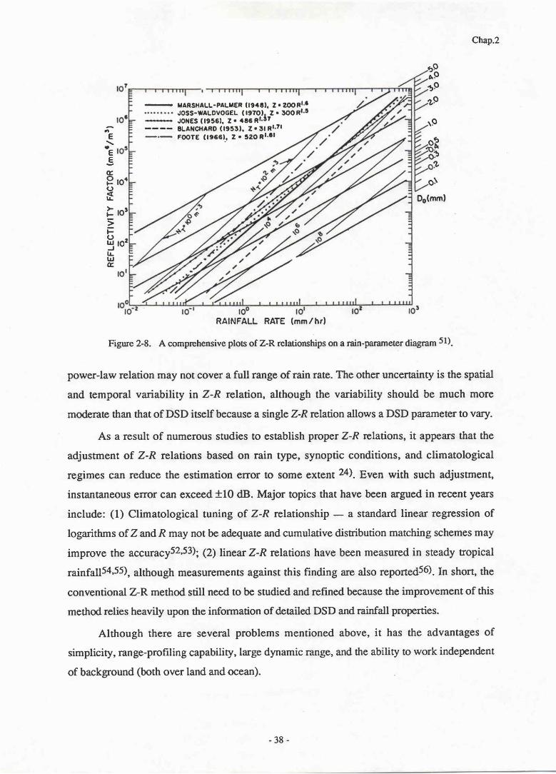
Chap.2
出i::‖よ:謂T:1::■::F°300N・5
8LANCHARD〔 1953). 2031R3.71
F00TE〔 1966〕.2・ 520 RI。●:
::う。
´
9ヽ
8:ひ
σ ♂ ♂
(”∈ヽ
oEE)にO卜0く」
ント一>一卜OuコLuC
多
0`
0。(mm)
RAINFALL RATE (mm / hr)
Figue 2-8. A comprehensive plots of Z-R relationships on a rain-parameter diagram 51).
power-law relation may not cover a full range of rain rate- The other uncertainty is the spatial
and temporal variability in Z-R relation, although the variability should be much more
moderate than that of DSD itself because a single Z-R relation allows a DSD parameter to vary.
As a result of numerous studies to establish proper Z-R relations, it appears that the
adjustment of Z-R relations based on rain type, synoptic conditions, and climatological
regimes can reduce the estimation error to some extent 24).Even with such adjustment,
instantaneous error can exceed +10 dB. Major topics that have been argued in recent years
include: (1) Climatological tuning of Z-R relationship - a standard linear regression of
logarithm s of Z and R may not be adequate and cumulative distribution matching schemes may
improve the accuracy52,53); Q) linear Z-R relations have been measured in steady tropical
rainfall54,55), although measurements against this finding are also reported56). In short, the
conventional Z-P. method still need to be studied and refined because the improvement of this
method relies heavily upon the information of detailed DSD and rainfall properties.
Although there are several problems mentioned above, it has the advantages of
simplicity, range-profiling capability, large dynamic range, and the ability to work independent
of background (both over land and ocean).
‐38-

Chap.2
2.3.6 Surface reference target (SRT) method
The SRT method, a methd to estimate path attenuation by using surface retrun as a
reference, was first proposed by Meneghini et a1.57) and has been recognized as a method that
has a potential to improve the spaceborne radar rainfall measurement accuracy to great extent;
by using this method alone or by combining it with other methods5S-63). The main reason is
that this methd can provide a rain rate estimate less sensitive to DSD variation than Z-R-
method. The second reason is that the path-integrated affenuation estimated from this method
can be combined with the Z-factor profile to improve the range-profitng accuracy as described
below. The derivation of path-integrated attenuation begins with a radar equation relating the
surface return power P1 to other par:rmeters in the presence of rain (the subscript I denotes the
quantities at the measurement in the presence of rain):
Pr = C1 r ;2 &1Aa1Ay (2.28)
where C is the radar constant, r is the range, and A7 and Aa represent path-integrated
attenuation due to rain and other factors, respectively. The constant C may vary depending on
the radar type and observation parameters. The problem is to estimate 47 from the
measurement of P1. One way is to measure a received power at an adjacent rain-free area or at
the same area as the raining region but before or after the rainin g, P2, which is given by
Pz - C2 r2-2 &zAo,2.
Then, taking the ratio of P1 to P2 gives
(2.2e)
(2.30)
The radar constant C is usually constant except for some variation in transmit power and
receiver gain which may be monitored, the range r can be measured accurately enough, and Ao
may be steady enough or negligibly small in comparison to Ar.If one can assume that o02 is
the same as oOt or the ratio is known, therefore, path-integrated rain attenuation A7 can be
calculated from 8q.2.30. It is clear from the above discussion that this method requires only
relative radar calibration and that d field should be homogeneous in space or steady in time.
The latter also suggests that this methd works fine for measurements over ocean with small
incidence angles at which wind speed and direction dependence of o0 is relatively small64).
Remaining uncertainties in this method include the contribution of bright band attenuation to
the total attenuation and the effects of raindrop striking the water surface656).
P1/P2=(C1/C2)(r2/rl)2(♂1/60"“α,lμα2)Are
-39 -
Chap.2
A dual-frequency version of the SRT methd (DSRT method) has also been proposed
by which a differential path attenuation can be estimated by taking the ratio of received powers
of two different frequencies. The DSRT method has the advantage that the accuracy in
attenuation estimate can be improved in proportion to the degree of correlation between ds at
the two frequencies 67).
2.3.7 Range profiling methods for attenuating-frequenc]' radar
The term "range profiling" means that rain rate or other rain parameters are to be
estimated as a function of range, perhaps with a range resolution within several hundreds of
meters. The Z-R method can serve as a range profiling method when no rain attenuation exists.
In heavy rainfall, however, the profile derived from the Z-R method would seriously under-
estimate the rain rate unless some attenuation correction is applied. Several methods have been
proposed to improve the attenuation correction accuracy.
A. Hitschfeld and Bordan (H-B) solution
If we can apply a single k-Ze relation, k = aZeF, for a path, the attenuating radar
equation ,8q.2.23, can be analyticalty solved for Ze as follows 68'69).
Ze(r) - zm(r)t 1 - 0.2 ln10 g f " zm{)Ftu l-16.
0(2.31)
This is known as the Hitschfetd-Bordan68) (H-B) solution. This exact solution, however,
tends to be very unstable when it is applied to cases of moderate to large attenuation because in
such cases errors in k-Ze relation and radar constants are amplifred significantly to cause very
erroneous solutions. Hitschfeld and Bordan68) suggested that the error should be reduced by
using a reference rain rate constraint farther deep in the storm.
B. H-B solwion with path-attenu.ation constraint
The constraint with rain gage data can be replaced by a path-integrated attenuation to
stabilize the solution to the attenuating radar equation as proposed by several researchers
57 ,62,70-72). There are some variations in the approaches taken to derive the rain rate and
attenuation profiles; however, the basic concepts can be summarized in the following two
points: (1) An "initial" value at the entrance of a storrn (received power data without
attenuation), or a "final" value at the range gate just above the surface (the 2-way path-
attenuation up to the range gate can be derived from the surface return) has to be used. While
- 4 0 -
Chap.2
the former condition is the same as the H-B solution, the latter provides much more stable
solution than the form e{2). (2) The path-integrated attenuation constrains the path-integrated
quantities derived from the Z-factor profile. A problem is that the attenuation at the bright band
or other hydrometeors aloft, at which k-Ze relations are not as clearly described as at rain
region, has to be taken into account.
C. Dffirerxial received power profile with puhetteruation constraint
Instead of Z-factor profile itself, Fujita6l) proposed to employ the ratio between
received powers at two adjacent range gates. Assuming power-law Ze-R and ft-R relations, wo
obtain a set of n-l equations that relates the received powers and rain rates at the two range
gates. The path-integrated rain rate derived from the SRT method or microwave radiometers is
then used to derive the rain rate profile of n range gates.
D. Problems in the metlnds B and C
Range-profiling methods described in B and C have advantages that the instability in the
original H-B solution can be solved. The other advantage is that the accuracy in rain rate
estimation can be improved through the use of attenuation having higher correlation with rain
rate than 2.1\ey essentially require only relative radar calibration because a path-attenuation
derived from the SRT method or from microwave radiometry is used as a reference. Flowever,
these methods also have several problems:
(1) Since they rely on the DSD insensitivity of rainrate-attenuation relationships, estimation of
rain parameters other than rain rate may have larger errors; e.g. estimating LWC.
(2) It may be difficult to use those methds over land and over ocean with large (>10")
incidence angles because of the difficulty to apply the SRT method-
(3) The non-uniformity in rainfall over the cross-beam FOV causes errors in estimating rain
rate and other rain parameters. It has been shown that the effects of the non-uniformity is more
serious in the SRT method than in the Z-R method73-7s). Thus, the applicability of these
methods is questionable for storms having a large non-uniformity (e.g. storrn edge).
2.3.8 DSD estimation methods
If we can estimate DSDs for each radar resolution volume, it would provide an "ideal"
remote sensing data because the DSD is a fundamental rainfall parameter to determine IRPs of
interest. However, it is very difficult to estimate the DSD profile precisely by remote sensing
techniques.
‐41-

Chap.2
In spite of the extensive work by Ulbrich and Athsl9), finle experimental work has been
conducted for estimating DSD profile except for the dual-polarization radar studies. The
difficulty of using dual-frequency radars for DSD estimation was addressed by Goldhirsh and
Ka1750,76). They assumed radars operating at (S and X bands), (S and K bands), and (X and
K bands) to measure (Ze andX-band attenuation), (Ze and K-band attenuation), and (X and
K-band attenuations), respectively, with the range resolution of I km. The radar reflectivity
should be uniform within this resolution to measure the attenuation from the decrease in range-
normalized received power. Although they conclude that an (S, K band) system may have an
acceptable accuracy, the above assumptions required for this method are not always satisfied.
The fundamental difficulty in this method is to measure an attenuation with a fairly high
resolution of 1 km or so, and therefore this type of dual-parameter radar measurements to
estimate DSD has not been considered as a practical system until now.
The DSD estimation methd we propose in this thesis is based on the following facts:
(1) The original dual-frequency method tries to estimate the DSD independently for each
resolution (- 1 km or less); however, it may be reasonable that DSD is correlated to some
extent in space so that estimating DSD with such a high resolution is not necessarily requted.
(2) The combination of low resolution (path-integrated) Z factor and attenuation measurements
can be employed to estimate a path-averaged DSD, if Z factor is measured without attenuation.
However, such path-averaged DSD is not sufficient for profiling of rain parameters.
(3) A reasonable resolution in the DSD estimation would lie between (1) and (2); i.e. one of
the DSD parameters varies with range gate but the other one is constant over the path. The
parameters of such a "two-scale" DSD model can be estimated from the combination of a high
resolution Z-factor and a low resolution attenuation measurements that has been used to
improve the rain rate profiling as mentioned above.
This two-scale model approach is expected to provide useful DSD information without
imposing strict radar system performance. In this sense, this method can be recognized as an
extension of the range profiling methods studied by several researchers for spaceborne radars
toward the original concept of DP measurement to estimate the DSD parametersl9'51). The
study of spatial and temporal DSD fluctuation properties is therefore important for developing
a method to estimate the parameters of the two-scale DSD model.
-42‐

Chap.2
2.3.9 Mirror image method
Meneghini and AtlasTT) proposed to utilize the "mirror" image of rain echo to derive a 4-
way path-attenuation. The advantage of this method is the increased sensitivity for light rain
and a potential to remove the unknown surface o0 from the algorithm by forming the ratio of
direct to mirror image returns. Tests have been conducted using the data from the CRLA.IASA
joint aircraft experimentTS). Although the test results are generalty encouraging, it is premature
to judge if this method is feasible or not. [t may provide another tool to make an SDP
measurement from space.
Appendix 2-L Bright Band Model
l. Composite Dielectrics Modcl
The bright band model used for this thesis is outlined betow referring to Awaka et al30).
As a first step, a composite dielectrics model is used to calculate the dielectric constant of the
bright band particle. We assume that bright band particle (snowflake) is composed of a
uniform mixture of water, ice and air. Dielectric constants of water, ice, air (t*, €i, and t",
respectively) are related to the dielectric constant of their mixture, i.e. snow, (es) with
sa -1(2.A1)
es+u ea+ u
where Uis aform factor, andPn,P;, and Poare fractional volume contents of water, ice and
air, respectively. By definitiorr, Pw+ Pt* Pa = 1. Also, letting Pw, Pi, and pa be the density
of water, ice and air, respectively, the density of snow, Ps, can be written
ps=ρ w P″ +pi P′+pa Pa・ (2.A^2)
Noting that p* = L glcm3, pi =O.92 glcml *d pu " 1 g/cm3, wo have Pi: (pt - PilO.9Z.
Since there is an empirical relation Ps = lp;33), we have the relation P; = ([Pn - Pi/0.92.
Noting that the last term of Eq. (2.A1) can be omitted because Ea= 1, and that e* andei are
uniquely determined by specifying the temperature of the particle,T, the quantities necessary
to determine the dielectric constant of snow, €s, are Pn,T, and U. Table z-AL lists those
parameters in the bright band as well as the resultant refractive indices of snow at several
frequencies.
t s - 1 €s7 -1 e i - 1-Pw +P t +Pa
Ew+U e i+U
- 4 3 -
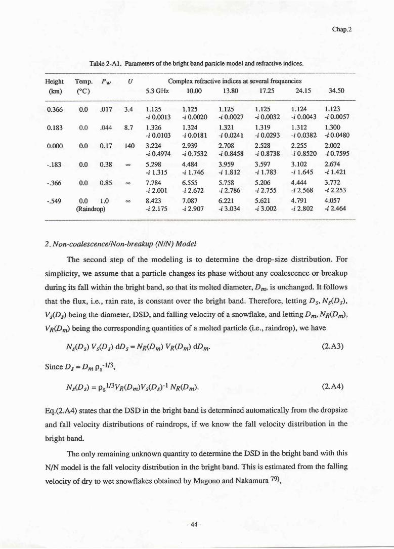
Chap.2
Table 2-Al. Parameters of the bright band particle model and refractive indices.
Hcight Temp. Pw
(kコn) (°C)
υ C o m p l e x r e f r a c d v e i n d i∝ s a t s e v e d f r e q u e n c i e s
5.3 GI・Iz 10。00 13.80 17.25 24.15 34.50
0.366
0。183
0 . 0 0 0
-.183
-.366
-.549
1.125‐JO。∞ 13
1.326‐JO。0103
3.224-JO.4974
5。298
‐Jl.315
7.784-′2 .∞1
8.423‐,2.175
1.125‐′0。0020
1.324‐li O . 0 1 8 1
2.939-li O.7532
4.484
-Jl.746
6.555-li 2.672
7.087-J2.907
1.125
■0。0 0 2 7
1.321- l i O . 0 2 4 1
2.708-li O.8458
3.959-′1.812
5.758- l i 2 . 7 8 6
6.221-J3.034
1.125‐jO.0032
1.319-′0。0293
2.528‐,0.8738
3.597‐′1.783
5。206‐J2.755
5。621-′3.002
1 . 1 2 4‐:0.0043
1.312-JO.0382
2.255-′0.8520
3.102‐′1.645
4.“И4‐′2.568
4.791-j2.802
1.123‐,0。0057
1.300-:0。0480
2.002-'0。7595
2.674‐Jl.421
3.772‐J2.253
4。057-J2.464
0。0 .017
8.7
0.0 0。17 140
0。0 0.38
0.0 0.85
0.0 1。 0
CaindrOp)
3.4
2. Non-coalescencelNon-breakup (N lN ) Model
The second step of the modeling is to determine the drop-size distribution. For
simplicity, we assume that a particle changes its phase without any coalescence or breakup
during its fall within the bright band, so that its melted diameter, D*, is unchanged. It follows
that the flux, i.e., rain rate, is constant over the bright band. Therefore, letting D", Nr(Dr),
Vr(Dr) being the diameter, DSD, and falling velocity of a snowflake, and letting D*, Nn(D^),
Vn(Dr) being the corresponding quantities of a melted particle (i.e., raindrop), we have
鳩 のs)ysの s)dD∫=」路 の“)yR(D″ )dD″ 。
Since Ds=D″ ps‐1/3,
鳩 の s)=ps1/3yR(D″)ysのs)~1域の“)。
(2.A3)
(2.A4)
W.Q.A ) states that the DSD in the bright band is determined automatically from the dropsize
and fall velocity distributions of raindrops, if we know the fall velocity distribution in the
bright band.
The only remaining unknown quantity to determine the DSD in the bright band with this
N/N model is the fall velocity distribution in the bright band. This is estimated from the falling
velocity of dry to wet snowflakes obtained by Magono and Nakamura 79),
-44-

ysのD=8.8x[0.lDKps― pD]1/2
Vs(Ds)=3。3x[ps― pa11/2
Chap.2
(0.05 s p, < 0.3 9c*3) (2.A5a)
(ps s 0.05 9c*3) (2.A5b)
and the falling velocity of raindrops, VR (see Section 2.L.4), using the following interpolation
scheme: Since usually ps > pa,Eq.(2.A5a) can be approximated as Vs - 2.8 P"LR'J/D^. (Note
that D, - Dmpr-16.) This means that the fall velocity of a snowflake having a given DpTis
proportional to ps-l/3 in the region, 0.05 S p, < 0.3 g/"*3. If we assume that this pt
dependence of the fatl velocity holds also in the region, 0.3 < Ps < L glcm3, the following
relation is obtained for a given Dp1:
Vs= f fn - Vsdx (ps l6 -0 .31 /3 ) | 4 t -0 .31 /3 ) +Vs7 (0 .3<ps< 1g l c *3 ) (2 .46 )
where Vsp is the fall velocity of a snowflake at ps = 0.3 g/r 3 grven by Eq.(2.A5a). Since
there is the relation ps = ,[Pn, the fall velocity distribution at a specified altitude can be
calculated from the Ptu data grven in Table 2-Al.
‐45‐

Chap.2
References
(1) Ray, P. S., 1972: Broadband complex refractive indices of ice and water.
Appl. Optics, 11, 1836- l84r'.(2) Meneghini, R. and T. Kozu, 1990: Spaceborne weather radar. Artech House, Norwood,
MA, 199pp.(3) Matsumoto, A. and A. Nishitsuji, eds., l97L: SFIF and EFIF propagation in snowy
districts, Morngraph Ser. of the Res. Inst. of Appl. Electricify, Hokkaido Univ., (19).
(4) Nishitsuji, A. and M. Hirayama,1971: On the anomalous attenuation of radio wave due
to snowfall. Trars. IECE Japan,s4-B, 22-29 (in Japanese).
(5) Pruppacher, H.R. and R.L. Pitter, L97l: A semi-empirical determination of the shape of
cloud and rain drops. J. Atmos. Sci., 28,86-94.
(6) Awaka, J., and T. Oguchi, 1982: Bistatic radarreflectivities of Pruppacher-and-Pitter
form raindrops at 14.3 and 5.33 GHz. J. Radio Res. Lab.,29, (127), 125-150.
(7) Stratton, J.A., I94L: Electromagrrctic theory, McGraw-Hill, New York.
(8) Oguchi, T., 1981: Scattering from hydrometeors: A survey. Radio Sci., L6,69I-730.
(9) , 1983: Electromagnetic wave propagation and scattering in rain and other
hydrometeors. Proc. IEEE, 7 L, IO29- 1078.
(10) Ulaby, F.T., R.K. Moore, and A.K. Fung, 1981: Microwave remote sensing: Active
and Passive. Vol.I. Artech House, Norwood, MA, 456pp.
(11) Gunn, K.L.S. and G.D. Kinzer, L949: The terminal velocity of fall for water droplets in
stagnant air. J. M eteorol., 6, 243-248.(L2) Foore, G.B. and P.S. du Toit, 1969: Terminal velocity of raindrops aloft.
J. Appl. Meteor.,8, 245-253.(13) Uplinger, W.G., 1981: A new formula for raindrop terminal velocity. Preprints,
20th Conf. Radar Meteor., Boston, MA, Amer. Meteor. Soc., 389-391.
(14) Atlas, D. and C.W. Ulbrich, L977: Path- and area-integrated rainfall measurement by
microwave attenuation in the 1-3 cm band. J. Appl. Meteor., L6, 1322-1331.
(15) Joss, J., J.C. Thams, and A. Waldvogel, 1968: The variation of raindrop size
distribution at Locarono, Proc. Int. Conf. Clottd Physics,369-373.
(16) Waldvogel, A., L974: The Ng jump of raindrop spectra.I. Atmos. Sci., 3L, LO67-1078-
(17) Feingold, G. and Z.l-evin, 1986: The lognormal fit to raindrop spectra from frontal
convective clouds in Israel. J. Climate Appl.Meteor.,25,1346-L363.
(18) Kozu, T. and K. Nakamura, L99l: Rainfall parameter estimation from dual radar
measurements combining reflectivity profile and path-integrated attenuation.
J. Atmos. Ocean. Tech.,8, 259-270.
(19) Arlas, D., C.W. Utbrich and R. Meneghini, 1984: The multiparameter remote
measurement of rainfall. Radio Sci. 19, 3-22.
(ZO) Chandrasekar, V. and V.N. Bringi, 1987: Simulation of radarreflectivity and surface
measurements of rainfatl. /. Atmos. Oceanic. Tech.,4,464-478.
(ZL) Feingold, G. and Z.l-evrn, 1987: Application of the lognormal raindrop size distribution
to diffelential reflectivity radar measurement (Znil. I. Atmos. Oceanic. Tech-,
4 ,377-382, .
‐46-

Chap.2
(22) Marshall, J.S. and W.M. Palmer, 1948: The distribution of raindrops with size.
f . Meteorol . ,s, 165-166.(23) Joss, J. and E.G. Gori, 1978: Shapes of raindrop size distributions. J. Appl. Meteorol.,
17, 1054-1061.(24) Stout, G.E. and E. A. Mueller, 1968: Survey of relationships between rainfall rate and
radar reflectivity in the measurement of precipitation. I . AppI. Meteor.,7 , 465-474.
(25) Battan, L.J.,1973: Radar obseryation of the atmosphere,The University of
Chicago Press, Chicago, 324pp.(26) Atlas, D. and C.W. Ulbrich, 1974: The physical basis for attenuation-rainfall
relationships and the measurement of rainfall parameten by combined attenuation
and radar methods, ,f. Res. Atmos.,8,275-298.(27) Ulbrich, C.W., 1983: Natural variations in the analytical form of raindrop size
distributions. J. Climate Appl. Meteor.,22, L764-1775.
(28) Dissanayake, A.W. and N.J. McEwan, L978: Radar and affenuation properties of rain
and bright band. IEE Conf. Pttbl. L69, 125-L29.
(29) Yokoyama, T., H. Tanaka, K. Nakamura, and J. Awaka, L984: Microphysical
processes of melting snowflakes detected by a two wavelength radar. Part II.
Application of a two-wavelength radar technique. J. Meteor. Soc. Japan,62,668-677 -
(30) Awaka, J., Y. Furuham&, M.Hoshiyama, and A. Nishitsuji, 1985: Model calculations
of scattering properties of spherical bright-band particles made of composite dielectrics.
J. Radio Res. Lab.,32, 73-87 .
(31) Bringi, V.N., R.M.Rasmussen, andJ. Vivekanandan, 1986: Multiparameterradar
measqrements in Colorado convective storrns. Part I: Graupel melting studies.
f . Atmos. Sci., 43, 2545-2563.(32) Klassen, W., 1988: Radar observations and simulation of the melting layer of
precipitation. J. Atmos. Sci., 45, 3741-3753-
(33) Wilheit, T.T., 1986: Some comments on passive microwave measurement of rain.
Bull. Amer. Meteor. 9oc.,67, 1226-1232-
(34) Kummerow, C., R.A. Mack, and I.M. Hakkarinen, 1989: A self-consistency approach
to improve microwave rainfall rate estimation from space. J. Appl. Meteorol.,
28, 869-884.(35) Capsoni, C., F. Fedi, and A. Paraboni, 1987: A comprehensive meteorologically
oriented methodology for the prediction of wave propagation parameters in
relecommunication applications beyond 10 GHz. Radio Sci., 22,387-393-
(36) Kummerow, C. and J.A. Weinman, 1988: Determining microwave brightness
temperarures from precipitating horizontally finite and vertically sb:ltctured clouds.
J. Geophys. Res., 93, (D4), 3720-3728.
(37) Oguchi, T., lg77: Scattering properties of Pruppacher-and-Pitter form raindrops and
cross polarization due to rain: Calculations at 11, 13, 19.3 and 34.8 GHz-
Radio Sci., L2, 4l-5I.
(3g) Marshall, J.S. and Hitschfeld, W., 1953: The interpretation of the fluctuating echo for
randomly distributed scatterers. Part I. Can. J. Phys.3I,962-994-
-47‐
Chap.2
(39) Kodaira, N., 1960: The characteristics of the averaged echo intensity received by the log-arithmic IF amplifrer. 8th Weather Radar Conf., Amer. Meteor. Soc., Boston, L2L-125.
(40) Joss, J., R. Cavalli and R. K. Crane,1974: Good agreement between theory andexperiment for attenuation data. J. Res. Atmos.,8,299-318.
(41) Atlas, D., D. Rosenfeld, and D.A. Short, 1990: The estimation of convective rainfall byarea integrals, 1. The theoretical and empirical basis. J. Geophys. Res.,95,(D3), 2153-2160.
(42) Rosenfeld, D., D. Atlas, ffid D.A. Short, 1990: The estimation of convective rainfall byarea integrals ,2. The height-area rainfall threshold (HART) method. J. Geophys. Res.,95, (D3), 2L6L-2L76.
(43) Doviak, R.J. and D.S. Zmic, 1984: Doppler radar and weather observations.Academic Press, Orlando, FL, 458pp.
(44) Rogers, R.R., t984: A review of multiparameter radar observations of precipitation.
Radio ^Sci., L9, 23-36.(45) Hall, M.P.M., 1984: A review of the application of multiple-parameter radar
measurement of precipitation, ibid, 37 -43.
(46) Furuham&, Y. and T. Ihara, 1981: Remote sensing of path-averaged raindrop sizedistribution from microwave scatterin g measurement s. I EEE T rans . Ante nnns .P ropag., AP-29, 27 5-281.
(47) Ishimaru, A., L978: Wave propagation and scattering in random media. Vol.2.,Academic Press, Orlando, FL, 572pp.
(48) Seliga, T.A. and V.N. Bringi, 1976: Potential use of radar differential reflectivity
measurements at orthogonal polarizations for measuring precipitation. J. Appl. Meteor.,2L, 257 -259.
(49) Holt, A.R., 1984: Some factors affecting the remote sensing of rain by polarization
diversity radar in the 3- to 35-GHz frequency range. Radio Sci., 19, 1399-L412.(50) Goldhirsh, J. and I.Katz, L974: Estimation of raindrop size distribution using multiple
wavelength radar systems. Radio Sci., 9,439-446.(51) Ulbrich, C.W. andD. Atlas: 1978: The rain parameterdiagram: Methods and
applications. J. Geophys. Res., 83, (C3), L3I9-1325.(52) Atlas, D., D. Rosenfeld, and D.B. Wolfl 1990: Climatologically tuned reflectivity-rain
rate relation and links to area-time integrals, J. Appl. Meteorol.,29, LL2O-1 135.(53) Rosenfeld, D., D.B. Wolff, and D. Atlas, I99L: Derivation of non-power law effective
Z-Rrelation by PDF matching methd" J. Appl. Meteorol., accepted for publication.
(54) List, R., 1988: A linear radar reflectivity-rainrate relationship for steady tropical rain.
J. Atmos. Sci., 45, 3564-3572.(55) Tawadzki, I. and M. de A. Antonio, 1988: Equilibrium raindrop size distributions in
tropical rain. J. Atmos. Sci., 45,3452-3459.(56) Willis, P.T. and P. Tattelman, 1989: Drop-size distributions associated with intense
rainfall. J. Appl. Meteorol., 28, 3-15.(57) Meneghini, R., J. Eckerman, and D. Atlas, 1983: Determination of rain rate from a
spaceborne radar using measurements of total attenuation,IEEE Trans. Geosci.
Remote Sens., GE-?L, 34-43.
- 4 8 -
Chap.2
(58) Fujita, M., K. Okamoto, S. Yoshikado, and K. Nakamura, 1985: Inference of rain rateprofile and path-integrated rain rate by an airborne microwave scatterometer. Radio Sci.20, 63L-642.
(59) Testud, J., P. Amayenc, and M. Marzoug, 1989: Stereo radar meteorology: A promising
technique to observe precipitation from a mobile platform.
J. Atmos. Ocean. Tech.,6, 89-108.(60) Kozu, T., R. Meneghini, W. C. Boncyk, K. Nakamura, and T. T. Wilheit, 1989:
Airborne radar and radiometer experiment for quantitative remote measurements
of rain. Proc.1GARSS89, Vancouver, Canada, L499-I5O2.(61) Fujita, M., 1989: An approach for rain rate profiling with a rain-attenuating frequency
radar under a constraint on path-integrated rain rate , Proc. GARSS89, Vancouver,
Canada, L49L-I494.(62) Marzoug, M. and P. Amayenc, 1991: Improved range profiling algorithm of rainfall
rate from a spaceborne radar with path-integrated attenuation constrainl
IEEE Trans. Geosci. Remote Sens., GE-29, 584-592.(63) Kozu, T., K. Nakamura, R. Meneghini and W.C. Boncyk, I99I: Dual-parameter
radar rainfatl measurement from space: A test result from an aircraft experiment.
IEEE Trans. Geosci. Remote Sens., GE-29, 690-703.(64) Masuko, H., K. Okamoto, M. Shimada and S. Niwa, 1986: Measurement of micro-
wave backscattering signatures of the ocean surface using X band and Ka band
airborne scatterometers", J. Geophys. Res.,9l, (Cl 1), 13065-13083.(65) Moore, R.K., Y.S. Yu, A.K. Fung, D. Kaneko, G.J. Dome, and R.E. Werp, L979:
Preliminary study of rain effects on radar scattering from water surfaces. IEEE J.
Oceanic Eng., OE-4, 31,-32.(66) Bliven, L.F. and G. Norcross, 1988: Effects of rainfall on scatterometer derived wind
speeds. Proc. GARSS88, Edinburgh, U.K., 565-566.(67) Meneghini, R., J.A. Jones and L. H. Gesell, 1987: Analysis of a dual-wavelength
surface reference radar technique", IEEE Trans. Geosci. Remote Sens.,
GE-25, 456-47 L.(68) Hitschfel{ W. and J. Bordan, 1954: Errors inherent in the radar measurement of rainfall
at attenuating wavelengths. J. Meteorol.,ll, 58-67.(69) Meneghini, R., 1978: Rain rate estimates for an attenuating radar. Radio Sci.,
13, 459-470.(70) Lin, H., M. Xin, and C. Wei, 1985: Ground-based remote sensing of LWC in cloud
and rainfall by a combined dual-wavelength radar-radiometer system.
Advances in Atmos. Sci., 2,93-103.
(71) Weinmatr, J.A., C. D. Kummerow, and C. S. Atwater, 1988: An algorithm to derive
precipitation profiles from a downward viewing radar and multi-frequency passive
radiometer. P roc. GARSS88, Edinburgh, U.K ., 229-234.(72) Meneghini, R. and K. Nakamura, 1990: Range profiling of the rain rate by an airborne
weather radar. Remote Sens. Environ, 31, 193-209.
‐49‐
Chap.2
(73) Nakamura, K., 1989: A comparison of the rain retrievals by backscattering measurement
and attenuation measunement. Preprints,24th Conf. Radar Meteorol., Tallahassee, FL,
Amer. Meteor. Soc., 689-692.(74) Amayenc, P., M. Marzoug andJ. Testud, 1989: Non uniform beam fillingeffects
in measurements of rainfall rate from a spaceborne radar. ibid, 569-572.(75) _, and _, 1990: Analysis of cross-beam resolution effects in rainfall
rate profile retrieval from a spaceborne radar. Proc. /GARSS'90,College Park, MD.,
433-436.
Q 6) Goldhirsh, J., L97 5: Improved error analysis in estimation of raindrop spectra, rain rate,
and liquid water content using multiple wavelength radars. IEEE Trans. Antennas
P rop ag., AP -24, 7 L8-7 20.(77) Meneghini, R. and D. Atlas, 1986: Simultan@us ocean cross section and rainfall meas-
urements from space with a nadir-looking radar. J. Atmos. Oceanic Tech.,3, 400-413.
(78) Meneghini, R. and K. Nakamura, 1988: Some characteristics of the mirror image rcturn
inrun.Tropical Rainfall Measurements, J.S. Theon and N. Fugono, eds. A. Deepak
Publ., Hampton, VA, 235-242.(79) Magono, C. and T. Nakamura, 1965: Aerodynamic studies of falling snowflakes.
J. Meteor. Soc. Japan,43, I39-I47.
‐50-
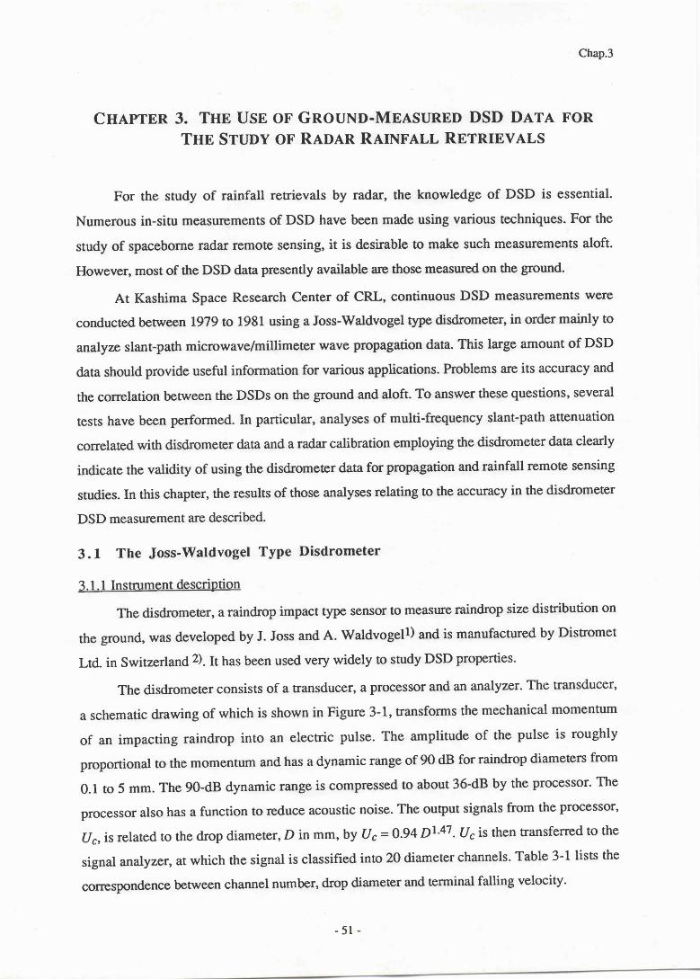
Chap.3
CHAPTER 3。 THE USE OF GROUND‐ MEASURED DSD DATA FOR
THE STUDY OF RADAR RAINFALL RETRIEVALS
For the study of rainfall retrievals by radat, the knowledge of DSD is essential.
Numerous in-situ measurements of DSD have been made using various techniques. For the
study of spaceborne radar remote sensing, it is desirable to make such measurements aloft.
However, most of the DSD data presently available are those measued on the ground.
At Kashima Space Research Center of CRL, continuous DSD measurements were
conducred between 1979 to 1981 using a Joss-Watdvogel type disdrometer, in order mainly to
analyze slant-path microwave/millimeter wave propagation data. This large amount of DSD
data should provide useful information for various applications. Problems are its accuracy and
the correlation between the DSDs on the ground and aloft. To answer these questions, several
tests have been performed. In particular, analyses of multi-frequency slant-path attenuation
correlated with disdrometer data and a radar calibration employlng the disdrometer data clearly
indicate the validity of using the disdrometer data for propagation and rainfall remote sensing
studies. In this chapter, the results of those analyses relating to the accuracy in the disdrometer
DSD measurement are described.
3. I The Joss-Waldvogel Type Disdrometer
3. 1. 1 Instnrment description
The disdrometer, a raindrop impact type sensor to measure raindrop size distribution on
the ground, was developed by J. Joss and A. Waldvogell) and is manufactured by Distromet
Ltd- in Switzerland 2). It has been used very widely to study DSD properties.
The disdrometer consists of a transducer, a processor and an analyzer. The transducer,
a schematic drawing of which is shown in Figure 3-1, ffansforms the mechanical momentum
of an impacting raindrop into an electric pulse. The amplitude of the pulse is roughly
proportional to the momentum and has a dynamic range of 90 dB for raindrop diameters from
0.1 to 5 mm. The 90-dB dynamic range is compressed to about 36-dB by the processor. The
processor also has a function to reduce acoustic noise. The output signals from the processor,
ur, is related to the drop diameter, D in ffif,, by ur=0.94 pt'47. ur is then transferred to the
signal analyzer, ar which the signal is classified into 20 diameter channels. Table 3-1 lists the
correspondence benveen channel number, drop diameter and terminal fatting velociry.
‐51
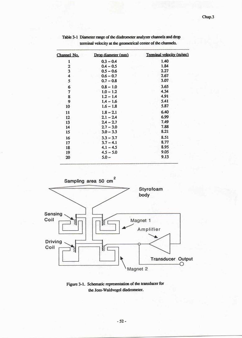
Chap.3
Tablo 3-l Dianreter range of the disdrcmecr analyzer chanrrls and &W
termind velocrty at fie geonrcrical cenrcr of thc channels
1
2
3
4
5
6
7
8
9
10
11
12
13
14
15
16
17
18
19
2 0
Q3‐ 04
04″ 05
0.5"06
0.6"Q7
0。7"08
0.8‐ 10
1.0″ 12
1。2″ 14
14-16
1。6‐ 1。8
1.8-2。1
21″ 24
2 4 - 2 7
27-3Ю
3。0~ 3。3
3。3-3.7
3。7″ 4.1
4。1″ 45
4。5-5Ю
5.0"
Sampling area 50 cm2
Styrofoam
body
SensingCo‖
Driv ingCoi!
Transducer Output
Figrge 3-1. Schernatfu reprcsartation of thc transdrrccr fc
the Joss-Wddvogel di*ometer-
1メ鋼D
l。14
227
2.67
3。07
3。6 5
4。3 4
4。91
541
5。87
6』
6。99
7“
7.88
821
8。51
8。77
8。95
9。05
9。13
‐52‐

3。
2。 5
2。
■.5
■。
0.5
0.5 ■ 。
乙σ= Σ (“j±q)D:6 + Σ “:D´Jこ{:∫″′≦8〕 iC〔お″j>8〕
h●=HdndДO角餞
■.5 2。
m/た
2.5 3
Chap.3
(3.1)
(3.2)
Figure 3-2. Distribution of normalized mQnln) of Poisson-distributed random process.
3.1.2 Sampling error
It has been shown that the total number of raindrops observed by a drop sampling
device under a uniform rain rate, n, is distributed according to the Poisson distribution3)
Π(れ,″)=C~“ ″・/“′
where rn is the mean value of the number of drops to be observed for a given sampling area
and period. The standard deviation of Poisson distribution is fi. We can also recognize that
Eq.3.1 is the probability of true mean m for a given observed number of drops n. The
probability of the normalized m (m/n) is shown in Figure 3-2for several n values. It is found
that sampling error is significant if the number of samples is less than about 10. Therefore,
data of large diameter disdrometer channels having less number of samples are generally more
erroneous than smaller drop diameter channels.
In order to assess the effect of such sampling error, a simple test has been made using
the measured disdrometer data. Let nibe the number of drops measured at channel i. For this
test, it is assumed that channels having ni greater than 8 measure the drops correctly and that
the tnre count number at the channels having n; equal to or smaller than 8 may be (ni + o;) or
(nt - o) with or -",[nr.The range of variation in 6th moment (Zfactor) is calculated by
4o is recognized as the Z values to be obtained if ttre dtop number observed is biased by oi.
‐53‐
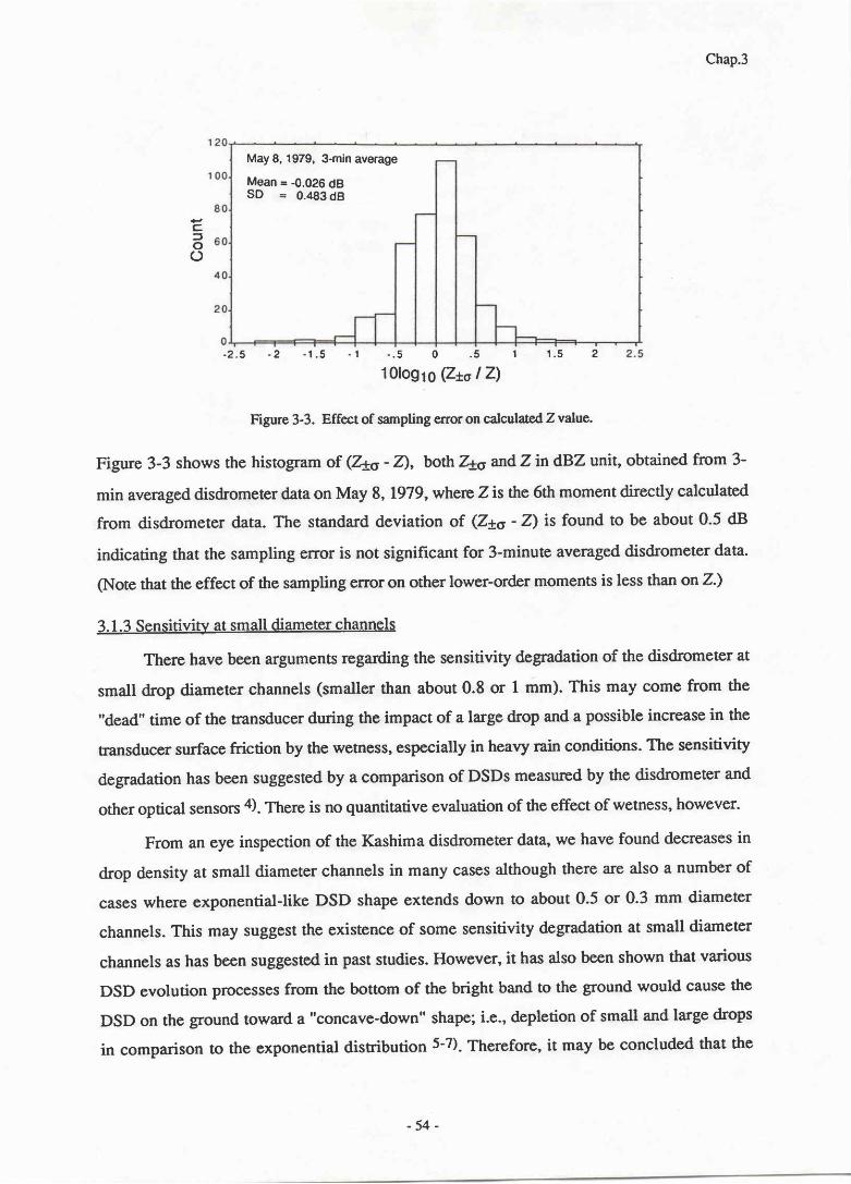
Chap.3
Figure 3-3. Effect of sampling error on calculated Zvalue.
Figure 3-3 shows the histogram of (Zxo - Z), both 4o ndZ in dBZ unit, obtained from 3-
min averaged disdrometer data on May 8, Lg7g,where Z is the 6th moment directly calculated
from disdrometer data. The standard deviation of (Zxo - Z) is found to be about 0.5 dB
indicating that the sampling error is not significant for 3-minute averaged disdrometer data.
(Note that the effect of the sampling error on other lower-order moments is less than on Z.)
3.1.3 Sensitiviqv at small diameter channels
There have been arguments regarding the sensitivity degradation of the disdrometer at
small drop diameter channels (smaller than about 0.8 or 1 mm). This may come from the
"dead" time of the transducer during the impact of a large drop and a possible increase in the
transducer surface friction by the wetness, especially in heavy rain conditions. The sensitivity
degradation has been suggested by a comparison of DSDs measured by the disdrometer and
other optical sensors 4). There is no quantitative evaluation of the effect of wetness, however-
From an eye inspection of the Kashima disdrometer data, we have found decreases in
drop density at small diameter channels in many cases although there are also a number of
cases where exponential-like DSD shape extends down to about 0.5 or 0.3 mm diameter
channels. This may suggest the existence of some sensitivity degradation at small diameter
channels as has been suggested in past studies. However, it has also been shown that various
DSD evolution processes from the bottom of the bright band to the ground would cause the
DSD on the ground toward a "concave-down" shape; i.e., depletion of small and large drops
in comparison to the exponential distribution 5-7). Therefore, it may be concluded that the
“Cコ00
May 8,19790 3‐ min average
Mean=_o.o26 dB
SD = o.483 dB
‐2.5 ‐ 2 ‐1.5 ‐ 1 ‐.5 0 .5 1 1.5 2
l o10gl。(zttσノZ)
‐54‐
Chap.3
depletion of small drops observed by the disdrometer represents natural DSD properties to
some extent.
In order to assess the effect of this uncertainty in DSD shape at the small drop
diameters, the following test is performed: We assume; that the DSD shape at the drop
diameter range less than 0.9 mm (channel #6) follows an exponential distribution which is
derived from a linear regression of diameter versus log of DSD weighted by the contribution of
each channel to rain rate; and that the disdrometer measures the DSD correctly for the channels
higher than #6. Examples of original and modified DSD's are shown in Figure 3-4. The
modified DSD is then used to calculate rain rate, Z, and other rain parameters, and the results
are comparcd with those obtained by the use of original DSD. Figure 3-5 shows the histogram
of 10.loE(YmodlY^"or), where I represents an IRP (moment or rain rate) and subscripts
"meas" and "mod" indicate the value for measured and modified DSDS, respectively. It is
found ttrat the exponentiation of DSD at small drop diameters makes large differences in lower
order moments but only a small or little difference in higher order moments. Considering that
the exponentiation of the DSD used in this test probably overestimate the density of small
drops to some extent, as discussed above, and that the DSD variation at intermediate to large
drops is a dominating factor causing the fluctuation in the relation between higher order
moments such as Z-R relation, we can conclude that the effect of uncertainty in the disdrometer
data at the small drop channels is minor as far as our primary interest is focused on higher
order moments such as R andZ.
3.2 DSD Measurement at Kashima
The disdrometer measurement at Kashima Space Research Center, CRL, started in May
1979 and was continued for several years; however, after the summer 1981., the sensitivity of
the instrument has been degraded (K. Nakamura, private communication). Therefore, data
from May 1979 until July 1981 are used in this study. The data consist of more than one
hundred thousand l-min integrated samples, aboutT}Vo of which have rain rate less than 1
mm/h. Since the rain rate range most important for climatological and hydrological studies is
from about 1 mm/h to about 50 mm/h, and since the data at light rain rates have larger
sampling error, we use the data having rain rates higher than 1 mm/h in this study. To reduce
‐55-

500
450
2 20 150
Moan diff。=2。93 dB
RMS drf. =3.35 dB
4 4R(M3,67)
Moan diff。=0。404 dB
RMS dlff. =0.475 dB
(b)MOdried DSD
ゝ
350
m O o r“ E 3 0 0
30 2 2 1 1
01234
101ogR,mod/R,meas)
M3 Mean di“
,=0.696 dB
RMS di“` =0.800 dB
01234
10bg(M6.mod/M6,meas)
Figure 3‐5。 Histott ofthe difFerence bemeen IRPs calcuhじ
d with
山c onglnal and modirled disdrometer dam。
Fig
ure
3-4.
E
xam
ple o
f dis
drom
eter
daa
mod
ifica
tion:
(a) O
rigrn
al,
O)
expo
nent
iatio
n at s
mal
l dro
p cha
nnel
s (< I
mm
).
( 0 一 ” o 0 0 事 L 〓 だ 」 0 0 〇 一 Φ > 〓 ● 一 0 』 ) C O 〓 C L C O ● E 0 0 a O ■ 日
一 C コ 0 0
‐ い い ‐50 450
4 3 3 250
200
1 1
012345
Diameter(mm)
012345
Diameter(mm)
O F ” ● ・い
(a)0百
ginal DSD
Mean diff・=0.099 dB
RMS drf. =o。
160 dB
150
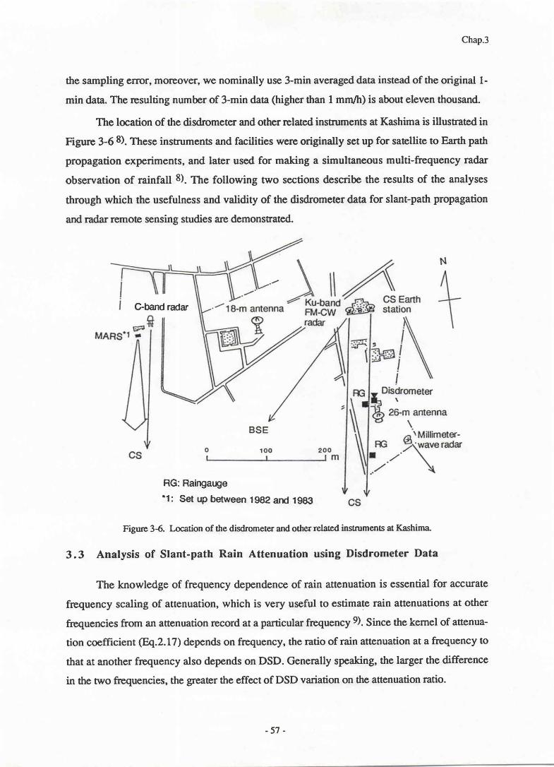
Chap.3
the sampling error, moreover, we nominally use 3-min averaged data instead of the original l-
min data. The resulting number of 3-min data (higher than I mm/h) is about eleven thousand.
The location of the disdrometer and other related instnrments at Kashima is illustrated in
Figure 3-6 8). These instnrments and facilities were originally set up for satellite to Earth path
propagation experiments, and later used for making a simultaneous multi-frequency radar
observation of rainfan 8). The following two sections describe the results of the analyses
through which the usefulness and validity of the disdrometer data for slant-path propagation
and radar remote sensing studies are demonstrated.
C-band radu
RG:Raingattle
・1: Set up between 1982 and 1983
Figure 36. Location of the disdrometer and other related instruments at l(ashima
3.3 Analysis of Slant-path Rain Attenuation using Disdrometer Data
The knowledge of frequency dependence of rain attenuation is essential for accurate
frequency scaling of attenuation, which is very useful to estimate rain attenuations at other
frequencies from an attenuation record at a particular frequency 9). Since the kernel of attenua-
tion coefficient @.2.17) depends on frequency, the ratio of rain attenuation at a frequency to
that at another frequency also depends on DSD. Generally speaking, the larger the difference
in the two ftequencies, the greater the effect of DSD variation on the attenuation ratio.
-57‐

Chap.3
A number of measurements of the attenuation ratio have been conducted both at
terrestrial and satellite-Earth linkslO-ls). In the case of the satellite link, analysis of measured
attenuation ratio is difficult because of the difficulty in obtaining detailed precipitation
properties on the slant path. Most of the slant-path propagation studies have described only
measured results and/or empirical formulas of the attenuation ratio, which have been shown to
vary widely from one rain event to another and within a rain event.
In the slant-path propagation experiments using CS and BSE satellites that we have
carried out at Kashima Space Research C-enter, a large amount of down-link beacon attenuation
data (CS 19.45 GHz, BSE 11.71 GHz) were obtainedlO. In addition, up-link attenuation data
were obtained simultaneous with the down-link data for more than ten rainfall events for both
CS and BSE. DSD's on the ground were also measured by the disdrometer.
In this section, the disdrometer-measured DSD data are employed for the analysis of
measured attenuation ratios, and the feasibility of slant-path attenuation ratio estimation by
ground-measured DSD data is examined. Because of the temporal and spatial discrepancies
between the propagation paths and the disdrometer site, one-to-one correspondence of
instantaneous attenuation values and disdrometer data may not give successful results.
Therefore, the present analysis deals with event-scale propertieslT).
Measurement parameters are summarized in Table 3-2. Up-link and down-link
frequencies are 14.4 and 1I.7 G}J.z for BSE and 28.9 and 19.5 GHz for CS. Signal levels
received at the ground station were sampled every second and stored on magnetic tapes. Slant-
path attenuations are obtained through the subtraction of received signal levels during rainfall
from those for clear weather estimated from the levels just before and after the rainfall and/or
those of the day following and preceding the rainfall day. It should be noted that a main point
Table3-2 Parameters for up-link and down-link acenuation measurements.
Frequency, up, GFIzFrequency, down, GFIzPolarizationSatellite Az, degSatellite El, degSatellite longitude, degDynamic range, up, dBDynamic range, down, dBSample rate, secAverage time, sec
B S E
14.36
11.71
Vertical
225
37
110
12
30
1
32
螢
28。85
19.45
Circular
189
48
135
18
35
1
32
‐58-

Chap.3
of this analysis is the use of two frequency attenuation data along the same propagation path
(i.e., each BSE and CS path), not the use of uplink and downlink signals.
3.3. 1 Event-scale attenuation ratio properties
It has been reported that Ze-R and k-Ze relations can be adjusted for each rain event
basis to give an improved accuracy in radar estimation of rain rate and attenuationl8'19).
Considering this fact, we examine event-scale attenuation properties.
To get an outline of event-to-event attenuation ratio variation, first we define the "event"
attenuation ratio (ARei by the slope of the best-fit regression line assumed to cross the origin;
ARιッ=Σ】ら2/Σ乃均ノ
where X7 and Yj are instantaneous values of down- and up-link attenuations (measured or
calculated from disdrometer data) for each rainfall event'. The other interpretation of AR", is
the average of instantaneous attenuation ratio with the weighting factor otXjYj; that is, greater
weight is given to larger attenuation values in the determination of ARrr, which is adequate for
most of practical purposes.
An example of AR* determination is shown in Figure 3-7.The left time charts show
measured and disdrometer (DM) derived attenuations. ARrr's for measured and DM-derived
attenuations are derived from respective instantaneous values by using 8q.3.3 as shown in the
right scattergftlms in Figure 3-7 . For comparison, another ARev is also calculated assuming the
Marshall-Palmer (MP) distribution 20). In this calculation, attenuation pairs are calculated from
the follo*ing 20 different MP distributions up to the maximum rain rate in that event(Ro*):
N(D) = 80O0 exp(-4.IRf .2n) with Rj = R*or 1g-0'08(20-i), i = I,2,...,20. (3.4)
These attenuation pairs are then used as the data for the regrcssion to obtain the ARev.
Figure 3-8 shows the scattergrams of measured ARev versus DM-derived and MP-
derivedARsy's. The result of the event attenuation ratio analysis is summarrzedin Table 3-3.
For BSE,, while the MP-estimated ARevhas little correlation with measured ARev, DM-derived
' A si-ilar quantity can be defined asD{iY1/D+2,which has been found to be very close to the value given by
8q.3.3 for all cases we have processed (within 27o)-
(3.3)
‐59‐
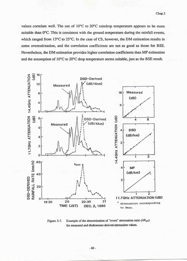
Chap.3
values correlate well. The use of 10"C to 20"C raindrop temperature appears to be more
suitable than 0"C. This is consistent with the ground temperature during the rainfall events,
which ranged from l3"C to 25"C. In the case of CS, however, the DM estimation results in
some overestirration, and the correlation coefficients are not as good as those for BSE.
Nevertheless, the DM estimation provides higher correlation coefficients than MP estimation
and the assumption of 10"C to 20"C drop temperatue seems suitable, just as the BSE result.
16
1 2
(mO) (口0)
Z〇一卜く⊃ZШトトく
N〓0寸.寸F ZOニトく⊃ZШトトく
N〓0卜err
Measured
DSD― Derived
1/′(oBノ4km)
′iЪ
20 20130 21
TIME(JST) DEC。 201980
Measured
(dB)
DSD
(dBノkm)
MP
(dBノ km)
11。7GHz ATTENUAT:ON(dB)
' AttenuatiOn COrresPOnding
to Rmax.
16
8
2
4
(口「)
ZO一卜く⊃ZШトトく
N〓0寸.寸”
4
2
(〓ヽEE)Ш卜く匡
コヨく」Z一く匡
口Ш>一匡ШO‥口のロ
60
4 0
20
19:30
Figure 3-7. Example of the determination of 'event" attenuation ratio (ARsy)
for measured and disdrometerderived auenuation values.
Measured
Rm譲:r l,1
1 1
ドヽ」 ヽ 、
6 0

Chap.3
1 . 9
呂1。7く∝
= 1。50ト
BSE
0°C
●● ●
・ノ/Ъ
・ ・
●
lo℃ .●
●
0/● ・
●
1 . 9
1。7
1 . 5
1.3
2.4
2.2
2.0
F。% / o00
MP0 ~~
(10° c)
2o"C ..1
● / ●
1.9
1.7
1。5
≦ 10刊lF¬高「~イ
ア~可
も 1・1 1.3 1。5 1。 7 1.9= 中
‐ ~
: CSく
0
世2.4く=
ぁ2.2田
2。0
2.0 2。 2 2.4 2。 0 2.2 2.4 2.0 2.2 2.4
MEASURED ATTENUAT:ON RAT:0
BSE
D
)℃) ・」∠′″ .
●
°/・
●
1。5 1。7
2.4
2.2
2。0
0
0
。S ∞
DSD
( 1 0 ° C )
1。5.31.91。7
針ILゴ計――乱一2
2 2 2
0
卜̈く∝
2〇
一卜くコZШトトく
OШ卜くΣ
卜̈のШ
1
00 2.2 2。4
MEASURED ATTENUATION RATIO
Figure 3-8. Uppen Scauergrams of measured vs. DMderived ,ARsyfordrop temperaurre of 0 - ?n"C.Lowen Comparison of correlations betrveen measured and DMderivedARay's andbetween AReis measured and estimated with the aszumption of lvlarshall-Palmer
DSD model.
264 2.22。0
0
。0 。
。ぽ
0°C
。0 ∞
。
0
S
,
0
10'C
OO C
。 20° C
0
00
0
MP
( 1 0° C )
● ●●
「θ・.
●・
‐61‐

Chap.3
Table 3-3 Summary of the event attenuation ratio (ARei analysis.
Raindrop temperature,DM estimation- oC
Raindrop temperahre,MP estimation- oC
10
B S E
Average difference
Correlation coeff icient
Avemgedifference
Correlation coefficient
‐0。047
0.760
0.314
0.376
‐0。023
0。764
0。2 0 0
0477
0.028
0。737
0。088
0.481
銀
-0。078
0 . 3 4 4
0.128
0 . 1 6 4
6
2
8
2
2
1
0】卜く∝ ZO】卜くコZШトトく
T人Ψ11
‘
―
The variability in instantaneous attenuation ratio within a rain event, which is a measure
of the validity of the event-scale attenuation ratio adjustment, is shown in Figure 3-9 together
with AR"u. Vertical bars in the figure indicate the maximum and the minimum values for
down-link attenuation larger than 2 dB. For BSE, it is found that attenuation ratios are
t mEAsuREDI um-oenrvED
6 6 8 8 4 51 4 2 9 2 0刃 コ 3/ 4
1979
‖ONTH′ DATE′ YEAR
{ **tu** | om-uentveo
6ユ
42
6■6卿
5■
52
1
5
・8
・98
5
7
2.2
ibl
8
4
1
1
O】卜く∝ 〓〇】卜くつZШトトく
BSE
Figure 3-9. Comparison of measured
and DMderived atrenuation ratios.
Open and solid circles denote
ARev, and heavy and light bars
show the maximum and minimum
values of instantaneous attenuation
ratios for downlink attenuation
larger than 2 dB.
7
82
1
7
2
981
4”
82
1 01 0 遇 」
I
椰
引
l 1
1
』』曇場1980
-62‐
1979
MONTH′ DATE′ YEAR
Chap.3
relatively stable within one event except for a strong convective stonns such as Augu st 24,
L979 and September 10, 1980, and that the measured and DM-derived attenuation ratio
variations correlate well. On the other hand, for CS, the correlation between measured and
DM-derived attenuation ratio variations is not as good as the result of BSE. The larger
variability in the measured values in CS suggests the existence of some causes of attenuation
other than rain or some height dependence of DSD.
3.3.2 Discussion on the measured and DM-derived attenuation ratios
In this section, we examine the cause of the disagreement (that measured values are
lower than the DM-derived ones) observed in the CS result. Similar results have also been
observed for the low-attenuation range (5 2 dB) of BSE.
Gaseotn atterut^ation: While the oxygen attenuation should be almost constant for rainy and
fine days, the difference in humidity between rainy and fine days2l) can contribute to the
attenuation ratio to small extent. The CS result can partly be explained by the water vapor
attenuation because the water vapor absorption at 19.5 GHzis larger than at28.9 GHz due to
the 22.235 GHz absorption line; however, this is not the case for BSE.
Bright band, attenuation: The other possible cause is the effect of bright band attenuation
and/or other DSD properties related to rainfall type, since most of the CS measurements were
made in stratiform rain. For BSE, no typical stratiform rain is included in the present analysis;
even if bright band is observed in the Z factor profile measured by the C-band radar22) (see
Figure 3-6), temporal variation in measurable attenuation is very large and spiky in most cases.
The bright band attenuation and attenuation ratio are calculated with the bright band
particle and its DSD model described in Chapter 2. Figure 3-10 shows the ratio of attenuation
cross sections (Q& of up- and down-link frequencies for raindrop and bright band particles.
As shown in this figure, QE's decrease with drop diametet, D, in general but have peaks at
particularD values. QE's are affected by drop temperature mainly in the smallD region- This
is because the temperature dependence of absorption cross section is larger than that of the
scattering cross section and because absorption mainly contributes to total attenuation in the
smallD region. There is a difference in the location of peaks between QE's of raindrops and
of bright band particles. Attenuation ratio may be lowered by the existence of bright band
attenuation if bright band particles of small and/or large diameter predominate. On the other
hand, it may be increased if intermediate-sized par:ticles do.
- 6 3 -

CS 28。
9/19.5 GHz
1020
2809/1905 GHz
10°C
205
BRIGHT BAND (BB)
1 2 3 4
DROP DIAMETER (mm)
100
1234
DROP DIAMETER (mm)
Fig
ure 3
-10.
Rat
io of
att
enua
tion cr
oss s
ectio
ns at tw
o di
ffer
ent fr
eque
ncie
s(Q
tR) a
s a fu
nctio
n of d
rop d
iam
eter
.
3.0
202
204
104
0 5 0 5 0 5
2 1 1 2 2 1
( ∝ ■ 0 ) 〓 0 【 卜 0 回 ∽ ― ∽ ∽ 〇 ∝ 0 コ く 卜 〇 卜 」 〇 〇 【 卜 く ∝
0 8 6
2 1 1
0 【 卜 く ∝ 〓 0 【 卜 く ⊃ 〓 国 ト ト く
RRAIN BsE
1404/11。
7
I・ 烹ン‐́‐́‐ TI
‖EASURED
1 3 5 10 20
RAINFALL RAttE (mmノh)
Fig
ure
3-1
1.
Re
suls
of s
lan
t-p
ath
a
tte
nu
atio
n
ratio
calc
ula
tion
: rain
-on
ly,
brig
ht-b
and-
only
, and t
oul (
incl
udin
g gas
atte
nuat
ion)
.0 , ” ● ・い
20°
C カチフ
〆 /ノ
"1 b
rr
14.“/1107 GHz
BRIGHT BAND (BB
Chap.3
Figure 3- I I shows rain-only, bright-band only, and total (including gaseous
attenuation) attenuation ratios as a function of rain rate for relatively tight rain region, where
the DSD of rain is assumed to be the MP distribution. Solid circles indicate the measured
attenuation ratios for rainfall events during which clear bright band was observed. Rain height
and bright band thickness are assumed to be 3 km and 0.5 km, respectively. For both CS and
BSE, attenuation dependences of total and bright-band attenuation ratios are closer to the
measured dependence than of rain-only cases.
Height dependcrrce of DSD: DSDs would change systematically during their falt. In the case
of stratiform rain, there have been a number of studies on this subjee15,7'23,24).11te physical
processes relating to the DSD evolution include: breakup, coalescence, evaporation, accretion,
etc. As a result of analytical and simulation studies, it is a consensus that the DSD shape in a
stratiform rain woutd be more "concave down" near the ground than aloftT). Therefore, the
attenuation ratio calculated from the disdrometer data may not represent the overall attenuation
ratio properties along the slant-path. That is, there may be larger number of large and small
drops aloft than on the ground. To study this height dependence of DSD in detail, wo have to
develop a method to esrimate the original DSD from the final DSD measured on the ground,
which is a complicated inverse problem. For an approximate evaluation of the DSD change
with height, DSD is modified by the same methd as used for the disdrometer sensitivity
degradation test (see 3.1.3) except that DSDs are exponentiated at both small and large drop
regions in this case. Such modification is qualitatively similar to the natural one occurring in
stratiform rains and the calculated attenuation ratio may be a limiting value considering the
continuous change in DSD from the exponential shape to the measured DSD on the ground.
The calculated attenuation ratio is generally smaller than that obtained from the original DM
data by about 0.05 to 0.15, which is consistent with the difference between the estimated
(total) and the measured attenuation ratios shown in Figure 3-11.
3.4 Ku-band FM-CW Radar Calibration using Disdrometer Data
3.4.1 Outline of the FM-CW radar
A Ku-band FM-CW radar was developed at Kashima Space Research Center in order
mainly to study microwave propagation characteristics for slant paths 25,26). The major
advantage of this radar for the propagation studies is that the radar signal is transmitted from
the same antenna installed for the propagation data acquisition such as receiving a satellite
‐65-

Chap.3
beacon signal and measuring slant-path brightness temperature, thereby enabling close com-
parative analyses of the radar and propagation data. The radar was originally developed as an
FM-CW type, and later a pulse-compression (PC) system was added to increase the sampling
rate. Another objective of the radar development is to evaluate quantitatively the perforrnance
of the radar system for rainfall observation because at that time no report and only a few rcport
have been published on the rain observation by FM-CW and PC radars, respectively.
Table 3-4 lvlajor parameters of FM-CW radar.
Center frequency
Polarization
Antenna
Diameter
Gain
HPBW
Ouput power
Frequency deviation
Modulation signal
Modulation frequency
Range resolution
Measurable mnge
Dynamic nmge
Numb. of indep. samples
Scan time
14.3625 GHz
VerticalTransmit Receive
l 3 m 3 0 c m
63.1 dB 29.0 dB
0.10" 4.6"
49.1 dBm7.5 MlIz p-p
Triangular
300 Hz
100 m
0.25 - 15 km
80dB- 300
60 sec
The major parameters of the radar is listed in Table 3-4. Basically the radar was
constructed by utilizing an FM-TV transmitter and a 13-m Cassegrain antenna installed for the
BSE (Broadcasting Satellite for Experimental Purposes) experiment 27). A 12.0-GHz sky
noise temperature and an 11.7-GHz BSE beacon signal (during the BSE experiment only)
were also measured by the same antenna. Since the beamwidth of the 13-m antenna is
extremely narrow (0.1"), it is safe to assume that the cross-beam non-uniformity of rain in a
resolution volume is negligible. The signal backscattered from rain is received by a 30-cm
parabolic antenna. This antenna size was selected so that the scattered signals from range gates
between 0.25 and 15 km, which include all the precipitation regions along the slant-path, can
be received without scanning the receiving antenna. In Appendix 3-I, a radar equation relevant
to this system is derived.
6

Chap.3
3.4.2 Calibration method
Absolute radar calibration is essential to obtain quantitative radar reflectivity that is
required to estimate microwave rain attenuation and rain rate. However, it is not easy to make
an accurate calibration because of a number of error sources, and an overall external calibration
using reference targets is usually required. One type of the reference targets is point targets
such as metal spheres and corner reflectors, scattering cross sections of which are calculated
accurately2Sl. A problem in using such point targets is that the radar equation for the point
target is different from that for volume targets. Some of system constants such as antenna
pattern and pulse width can not be calibrated with the use of the point target. The most direct
way to make the overall rain radar calibration is to use rain itself as a reference target.
Therefore, this scheme has been widely used in spite of several error sources. The usual
method in this scheme is to compare the rain rates as measured by ground-based rain gages
and those estimated from the radar assumin g aZe-R relation. Clearly, there are two major eror
sources in this method. One is the spatial discrepancy between the observing volume by radar
and that by the gages; and the other is the uncertainty in Ze-R relation or DSD.
In order to reduce those errors, a new scheme has been developed for calibrating the
FM-CW radar. The main points are: 1) Path attenuation derived from a satellite beacon signal
or from the 12-GHz radiometer is used as a reference instead of raingage data; and 2) the
relation between attenuation coefficient versus Ze (k-Ze relation) derived from the disdrometer
data is employed for estimating slant-path attenuation, which is compared with the radiometer-
derived path attenuation to obtain a correction factor of the radar system constant, F.
As described in Chapter 2 @q.2.24) , the radar equation including attenuation effect on
received power is
c lKwlzPyQ)- - -Zm
12
(3.5)
where the radar constant C, which was given in Eq.2 .24 for a typical radar configuration, may
have a different form in this case, and is expressed by the "original" or uncalibrated radar
constant, C0, and a correction factor, F, as C - Co/F. A flowchart of the calibration is shown
in Figure 3-L2. The reference quantity,ll.7-GHz path-attenuation derived from the L2-GHz
sky noise temperature (Anu), was calibrated using the BSE beacon attenuation 29). Whereas,
-67 -

Sky noisetemp.
COノr2
Comparison
Chap.3
Disdrometer Radar Radiometer Beaconlevel
(TEE
”3E)
20
卜̈く匡卜Z口OZ00
Ш〓⊃JO>
LO∝O
LO
Or00J
Figure 3-12. Flowchart of radar calibration.
June 14, 1981 (Evel)
4
3
2
1
0 1234 %
Yes
1 2 3
(Ev.2)
、`\■830-■=39JST
4.■4mm/h
4
3
2
1
0
4
3
2
1
0
July 23-24, 198.1
t i r z l :30 -23 :39Js r
0。95mm/h
Q
4
3
2
1
0
RAINDROP D:AMETER(mm)
Figlre 3‐13。 Exalnple of disdrometer‐ measured DSDs during Ev。 l and Ev.2.
B r o k e n a n d d o t―d a s h l i n e s s h o w M P a n d J―D d i s m b u t i o n。
ヽヽ
゛9840-9849JsT
2。30mm/h
``い`l1820-■0829JsT `4。67mm/h
ヾ
‐68-
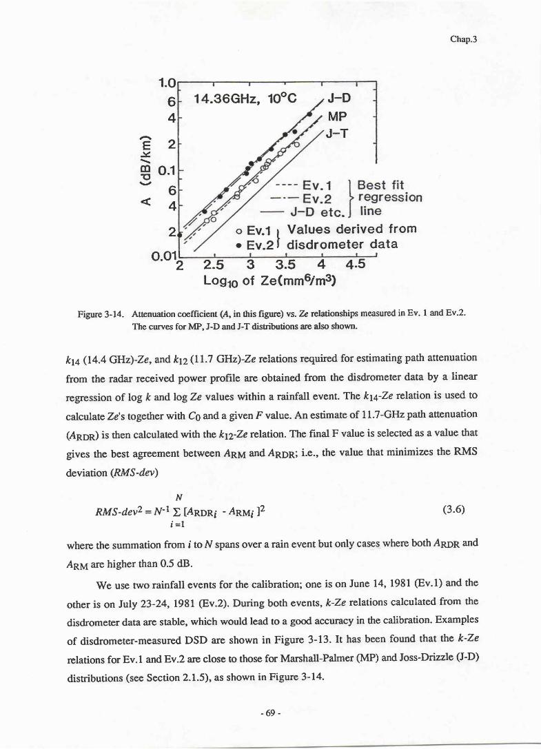
(E〓ヽmO)
く
1。0
6
4
2
0。1
6
4
2
14.36GH2, lOoC J―D
MP
J―T
2。5 3 3。 5 4 4。 5
Chap.3
(3.6)
:EILII二::「ビhli」IttElil°m
0。01生Loglo of ze(mm6/m3)
Figure 3-14. Attenuation coefficient (A, in this ngure) vs.7z relationships measured in Ev. I andEv.2.The curves for MP, J-D and J-T distributions are also shown.
ku Q4.4 GHz)-Ze, and kn(L1.7 GHz)-Ze relations required for estimating path attenuation
from the radar received power profile are obtained from the disdrometer data by a linear
regression of log k and log Ze values within a rainfall event. The &1a-Ze relatron is used to
calculate Zls together with CO and a given F value. An estimate of 11.7-GHz path attenuation
(Anoil is then calculated wirh the kp-Ze relation. The final F value is selected as a value that
gives the best agreement between ARU and AppR; i.e., the value that minimizes the RMS
deviation (RMS- dev)
J V
Rル「S―ご̀ッ2=ハルl Σ IARDR:―ARMI]2
′=1
where the summation from i to N spans over a rain event but only cases where both Appp and
Anu are higher than 0.5 dB.
We use two rainfall events for the calibration; one is on June 14, 1981 (8v.1) and the
orher is on July 23-24,1981 (8v.2). During both events, k-Ze relations calculated from the
disdrometer data are stable, which would lead to a good accuracy in the calibration. Examples
of disdrometer-measured DSD are shown in Figure 3-13. It has been found that the k-Ze
relations for Ev. 1 and Ev.2 are close to those for Marshall-Palmer (MP) and Joss -Drizzle (J-D)
distributions (see Section 2.1.5), as shown in Figute 3-14.
-69‐
Chap.3
One problem in the derivation of path-attenuation from radar is how to evaluate the
attenuation due to bright band particles. Goldhirshl9) obtained the best result for stratiform rain
when he omitted the bright band attenuation in his analysis using an S-band radar data. As
Dissanayake and McEwan 30) pointed out, this may be due to the fact that the increase in S-
band Ze atbright band is so large that the attenuation is significantly overestimated when the
same k-Ze relation as that for rain is used for bright band. However, the degree of the
overestimation should be relaxed with increasing frequency; the same k-Ze relation may be
applied both to rain and bright band when we use an X-band radar 30). For the Ku-band radar,
we calculate the bright band attenuation employing the particle and DSD models described in
Chapter 2.Theresultant k-Ze relation for the values averaged over the bright band is found to
give somewhat (about 1.5 times) larger attenuation coefficients than that for rain for a given
h. However, the properties of bright band particles still need clarification and the bright band
k-7n, relation may vary from case to case. Therefore, the following three k-Ze relations are
used for the evaluation of bright band attenuation: (1) no attenuation at bright band; (2) the
same k-Ze relation as that for rain; and (3) the above mentioned bright band k-Ze relation.
3.4.3 Result of the calibration
Figure 3-15 shows the relation between the RMS-deviation and F value used to
calculate ARpR. The curves designated as "DSD-Ev" represent the results using the
disdrometer-derived k-Ze relations. For comparison, the results using the k-Ze relations for J-
D, Mp and Joss-Thunderstorm (J-T) distributions are also plotted in the figure. The F value
that gives the minimum RMS-deviation for each curve, F6, differs by about 2 dB for each
event when J-D, MP or J-T distribution is assumed for both rain events. On the other hand,
Fp is almost constant when the disdrometer data are employed for estimating event-scale k-Ze
relations. This indicates the usefulness of disdrometer data to estimate DSDS on slant paths-
For Ev.l, about l-dB difference appears between the DSD-Ev Fp values obtained from the
assumption of bright band artenuation ( 1) and (3), while for Ev .2, the difference is only about
0.3 dB. This is due to rhe difference in the magnitude of bright band Ze'sbetween Ev.t and
Ev.2.However, it appears that the large event-by-event variability in DSD causes much larger
error in estimating Fm than the uncertainty in evaluating bright band attenuation-
Consequently, we have chosen F = L 5 dB for the FM-CW radar.
- 7 0 -
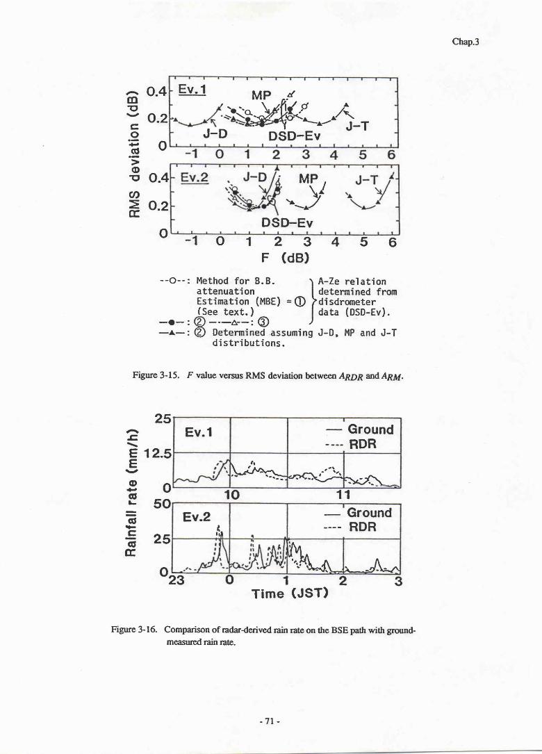
Chap.3
0。4
0。2
0
0.4
0。2
0▼ -1 0 1 2
F(
―-0‐―: Method for BcB.
attenuatlon
Estimatlon (MBE)
=ξ 電 淋 lpぷ sdistrlbutions.
Figure 3-15. F value versus RMS deviation betwee,n AnOn andApy.
Ev.1 GroundRDR
ー
10
25
0掟1 2
Time(JST)
Figure 3-16. Comparison of radarderived rain rate on the BSE path with ground-measured rain rate.
Ev。l MP ^〆
4TJ―D DSD― Ev
(口0)CO〓C一>00 ∽Σ匡
6
om
・
“丁
on
fr
v,
J
・l
r
rヒ
H一
5
)
‐at
ned
ete
SD一
an
re.m
romfD)MP
4
・Ze
eteisd
ata
・D,
A
d
d
d
J
30 、(L「り¨
(〓ヽEE)Φ一c』
「̈いE”∝
25
12。5
0
5011
30
↓DSD― Ev
Ev.21
‐―
GroundRDR
嘱
-71‐

Chap.3
To verify the calibration result, comparisons are made between rain rates measured by a
raingage and those from the calibrated radar data using the Ze-R relation derived from the
disdrometer. The rain gage is installed at about 2 km from the radar and about 1.5 km below
the BSE propagation path. Figure 3-16 shows the comparison of rain rates derived from the
radar reflectivity at the range bin just above the rain gage and those measured by the rain gage.
Several minutes' shifts of the time at which peaks of rain rates occur are probably due to the
1.5-km height difference. Including these time shifts, the radar derived rain rates are very
consistent with the rain gage data for both events.
3 .5 Conc lus ions
We have examined the validity to use DSDs measured on the ground by a disdrometer
for studying spaceborne radar rainfall measurements. Sampling errors and possible sensitivity
degradation of the disdrometer were examined It was found that those errors are not negligible
but the uncertainty in the measured DSD due to those errors are much smaller than natural DSD
variabilities.
We have used the disdrometer data to analyze the slant-path rain attenuation ratios and to
improve the accuracy in the calibration of the radar for rain measurement on a slant-path. It
was found that the event-averaged affenuation ratios are well correlated with the values
estimated from the disdrometer data, and that a reasonable radar calibration result is obtained
by the use of disdrometer-derivedk-Ze relations. Although a correction may be required for
the attenuation caused by the bright band in the case of stratiform rain and further study may be
required to model a height dependence of DSD shape, the results of these studies indicate the
validity of using the disdrometer data not only for ground based radar studies but also for
aircraft and spaceborne radar studies.
In the above studies, successful results have been obtained by employing the
disdrometer data to estimate event-scale relations between rain parameters such as attenuation
ratio and k-Ze relation. This suggests that the magnitude of the event-by-event variability in
DSD, which can be estimated from the disdrometer measurement, is a dominating factor to
determine the total variability of rain parameter relations rather than other sources such as
short-term or small scale variations of DSD within a rain event, height dependence of DSD and
effects of bright band attenuation. It may therefore be possible to model the rainfall in such a
way that some of the rain parameters vary more slowly than the variability in rain rate andZe-
- 7 2 -

Chap.3
Appendix 3-1: Derivation of radar equation for the Ku-band FM-CW radar
As shown in Figure 3-A1, we consider a cylindrical scattering volume LV the length of
which is equal to the range resolution, Ar, and we assume that the rain in AV is uniform and
that all of the power transmitted forward pass through the cross section of AV, S. Since the
beamwidth of the receiving antenna (4.6') is much wider than that of the transmitting antenna
(0.1"), receiving antenna gain (Gr) can be approximated to be constant over the AV. The
power of the received signal, P(r), scattered from raindrops in AV is expressed as
r■Ar/ 2
P(r)=('V4π)2.Gr ∫ :is(26むl「2d″r―Ar/2
( 3 ◆A l )
where 1, is the radar wavelength, r is the distance from the radar to the center of A% q is the
back-scattering cross section of rain per unit volume, and Q is the power flux density
illuminating an infinitesimal volume dV 1= ds dw) at the distance w. Rain attenuation along the
path has been neglected-
dV=dSOdW
→
BOresight
axis
Figure 3-Al. Scattering volume AV for the calculation of radar received power.
Lア一卜U、
‐73‐

Chap.3
From the above assumption, the surface integral of Q on S is almost equal to the
effective transmitted power EpnEbcing the antenna efficierrcy. Thus, when r > Lr,Eq.3.Al is
approximatcd as
Po~ aV4o2.Gr″ :Arノr2=メ lKJ々16■2)‐l GrもP′Ar盈 /r2 (3。A2)
wherc lKrl and Ze arc defrned in Table 2-l (also by Eqs.2.10 and 221). A merit to use a wide
beamwidttt receiving antcnna is that rreittrer transmiuing antenna gain ntr pattern appears in the
radar equation because almost all uansmitted power can be rwived by the receiving antenna
with approximatcly a constant gain, Gr. This means that the above radar equation worls even
in a near field regton. Substituting lKpll = 0.93, X = 2.O9 cm, G7 = 29.O dB and ?, = 6.4
dBm (6 = 0.54), which are the parameters of the FM-CW tadar, nrc have
P(r) (dBm) = -128.4 - 20 log r + 10 log Ar + 10lo9zc(r')
where units of a &, and Ze are km, m, and mm6/m3, reqlectively.
(3.A3)
-74 -
Chap.3
References
(1) Joss, J. and A. Waldvogel, L967: Ein Spektrograph fur Neiderschlagstropher mit
Automatischer Auswertung. Pure Appl. Geophys., 68, 240-246.
(2) Distromet Ltd.: Distrometer RD-69 ard Analyzer AD-69 Instruction Marurals.
P.O. Box 33, CH-402O Bassel, Switzerland.(3) Cornford, S.G., 1967: Sampling errors in measurements of raindrop and cloud droplet
concentrations. M eteor. Mag., 96, 27 L-282.(4) List, R., 1988: A linear radar reflectivity-rainrate relationship for steady tropical rain.
J. Atmos. .Sci., 45, 3564-3572.(5) Caton, P.G.F., L966: A study of raindrop-size distributions in the free atmosphere.
Quart. J. Roy. Meteor.|oc.,92, L5-30.
(6) Cataneo, R. and G.E. Stout, 1968: Raindrop-size distributions in humid continental
climates, and associated rainfall rate-radar reflectivity relationships. J. Appl. Meteor.,
7 , 90t-907.(7) Ulbrich, C.W., 1983: Nanrral variations in the analytical form of the raindrop size
distribution., J. Climnte Appl. Meteor.,22, 1764-L775.
(8) Nakamura, K., H. Inomata, T. Kozu, J. Awaka, and K. Okamoto, 1990: Rain observa-
tion by an X- and Ka-band dual-wavelength radar. J. Met. Soc. Japan,68, 509-52L.
(9) CCIR, 1990: Propagation data and prediction methods required for Earth-space
telecommunication systems. Report 5 64-3, Dusseldorf.
(10) Ippolito, L.J., l97I: Effects of precipitation on 15.3- and 31.65 GHz Earth-space
transmissions with the ATS-V satellite. Proc.IEEE,59, 189-205.
(11) Howell, R.G., J. Thirlwell, and N.G. Golfin, 1977: Simultaneous 20 and 30 GHz
attenuation measurements on a satellite-Earth path. Electron. Lett., L3, (2L),640-&2-
(12) Fang, A.J., and J. M. Harris, 1979: Precipitation attenuation studies based on measure-
ments of ATS- 6 20130-GHz beacon signals at Clarksburg, MD. IEEE Trans. Antennns
Propagat., AP-27 , 1'-lI.
(13) Nackoney, O.G., and D. Davidson, 1979: Rain attenuation of 12/1'4 GHz satellite
video transmissions. Electron. Lett., 15 (22), 703-7 04-
(14) Thirlwell, J., and R.G. Howell, 1981: Slant-path attenuation measurements in the range
12-30 GHz using OTS and passive radiometers at Martlesham Heath, England.
IEE Conf. Pub|.,195, 29-35.(15) Altshuler, 8.8., and L.E. Telford, 1980: Frequency dependence of slant path rain
attenuation at 15 and 35 GHz. Radio Sci. 15, 78t-796.
(16) Fukuchi, H., T. Kozu, K. Nakamura, J. Awaka, H. Inomata, and Y. Otsu, 1983:
Centimeter wave propagation experiments using the beacon signals of CS and
BSE satellites . IEEE Trans. Antennas Propag., AP-31, 603-613.
(17) Kozu, T., J. Awaka, H. Fukuchi, and K. Nakamura, 1988: Rain attenuation ratios on
30/20- and, 14/ l2-GHz satellite-to-Earth paths. Radio Sci., 23, 409-4 1 8.
(18) Srout, G.E. andE. A. Mueller, 1968: Survey of relationships between rainfallrate and
radar reflectivity in the measurement of precipitation. J . AppI. Meteor., 7 , 465-47 4-
7̈5-

Chap.3
(19) Goldhirsh, J., 1979: Predictive methods for rain attenuation using radar and in-situ
measurements tested against the 28-GHz COMSTAR beacon signal. IEEETrans.
Antennas Propag., AP-27, 398-406.(20) Marshall, J.S. andW.M. Palmer, 1948: The distribution of raindrops with size.
J. Meteorol.,s, 165-L66.(2L) Itoh, S., 1987: A method for estimating atmospheric attenuation on Earttr-space paths
in fair and rainy weather. Trans. IEICE Japan, J70-8, 1407-L4L4, (in Japanese).
(22) Tanaka, H., T. Shinozuka, K. Nakamura, K. Koike, and H. Kuroiwa, 1980:
ETS-II experiments, Part II, weather radar system. IEEE Trans. Aerosp. Electron.
Sysr. , AES-16, 567-580.(23) Srivastava, R.C. ,1971: Size distribution of raindrops generated by their breakup and
coalescence. J. Atmos. Sci., 28, 4LO-4I5-
(24) Brazier-Smith, P.R., S.G. Jennings, and J. Latham,1973: The influence of evaporation
and drop-interactions on a rainshaft. Qu"art. J. Roy. Meteor. 9oc.,99,704-722.
(25) Kozu, T., K. Nakamura, J. Awaka, and M. Takeuchi, 1983: L4-GHz FM-CW radar for
observation of precipitatron.Trans. IECE Japan, J66-8, L394-1401 (in Japanese).
(26) -, -, -, and -, 1987: Development of Ku-band FM-CWPulse-compres-
sion radar for rain observation on a slant-path. jf. Radio Res. Lab.,34, (L43), 95-113.
(27) Imai, N., Y. Otsu, and T. Tanaka, 1980: Main transmit and receive station in Japanese
BSE program. IEEE MTT-S Int. Microwave Symp., Washington, D.C.,281'283.
(28) Ulaby, F.T., R.K. Moore, and A.K. Fung, 1982: Microwave rentote sensing:
Active and Passive. Vot.[. Artech House, Norwood, MA, 457-1064pp.
(29) Kozu, T., H. Fukuchi, ild Y. Otsu, 1986: Comparison of antenna noise temperature
with rain affenuation of a satellite beacon signal at lzGHz. Electron. Lett.,zz, (24),
r27 4-127 5.(30) Dissanayake, A.W. and N.J. McEwan, L978: Radar and attenuation properties of rain
and bright band. IEE Conf. Pttbl.169, L25-L29.
‐76‐

Chap.4
CHapTBR 4. STnTTSTICAL PNOPBRTIES OF DSD PANAMETERS
Natural DSDs are highly variable; however, it is known that they can be modeled
reasonabty well by three-parameter models such as girmma and lognormal models. In this
chapter, we show the result of statistical properties of the gamma and lognormal DSD
parameters derived from the Kashima disdrometer data described in Chapter 3- The
knowledge of statistical properties of such DSD parirmeters are required to assess the values
derived from a remote sensing technique, to make further modeling of DSD in terms of rain
rate or Z factor dependences, temporal or spatial variations, and reducing the three-parameter
model to a two-parameter model. Those modeling may provide a better accuracy in a wide
ftrnge of radar rainfall measurements as well. Statistical analyses in this chapter include:
(1) Statisrics of parameters of the gamma and lognormal DSD models; (2) rain rute andZ-
factor dependences of the DSD parirmeters; (3) correlations among the DSD parameters; and
(4) statistics of IRP relationships. We also check the validity of using the gamma and the log-
normal models by means of a comparison of rain rates directly calculated from the
disdrometer data and from estimated DSDs. There are several time scales in statistical
analyses; long term (a season - it year) and short term (one rainfall event or less). In this
chapter, we mainly deal with the long term statistics. The short term statistics will be studied
in Chapter 5.
4.L DSD Models and the Parameter Estimation Methods
We use gamma and lognormal distributions both of which have been used for the
modeling of DSD (e.g. Ulbrichl) and Feingold and Levin2)). Especially, the gamma
distribution has extensively been used in recent years as an alternative of the conventional
exponential distribution. The gamma and lognormal models are given by
Ⅳ09)=式 、D″ exp(―妙 )=Ⅳ r='ギ1;‖1言「
eXP(―AD)
Ⅳα9)= 落走λ√万亮i exp(~ )
(4.la)
(4.lb)
where D is drop diameter, f(x) is the complete gamma function, [Ng, m and A] or fNr, m
and A] are parameters of the gamma model, and [N1, p and o] are parameters of the
-77‐

Chap.4
lognormal model. The parameters ,??+1 and n-l are also called the shape parameter and the
scale pammeter, respectively. Although ttre par:rmeter Nn zeroth moment of the gamma or the
lognormal model, is also recognized as an integral rain parameter ([RP), we treat it as a DSD
parameter as well. Note that the zeroth moment of actual DSD is generally different from the
parameter Nr obtained from the parameterization.
To estimate those DSD parameters from the disdrometer data, several methods have
been employed; fitting the measured DSD directly with some weightin *'3), Maximum
Likelihood Estimation (MLE)4'5), and Method of Moment (MoM;6'21. Although MLE is
considered to provide more stable estimates than others, it is not practical for the estimation
using remote sensing data because actual DSD samples are rcquired for this method. (fhe
same problem applies to the direct fitting method.) Since most remote sensing data are IRPs
approximately proportional to moments of DSD, MoM is considered to provide the estimates
most resemble to those obtained from actual radar measurements. A variery of combinations
of the moments can be used for the DSD parameter estimation. Although the conventional
MoM uses gth, lst and 2nd moments, for the present study, wo use higher order moments;
attenuation and Z factor approximated by 3rd and 4th moments for attenuation and 6th
moment forZ factor. The assumption for attenuation coffesponds to the siruation in which
rain attenuations are measured at two different frequencies; around} GHz and a millimeter
wave (see Figure 2-3). Although using a millimeter-wave radar seems to be difficult at
prcsent, this may not be the case in the futureS). For the DP measurement, we assume that
only 4th and 6th moments are measured. For more precise radar measurement simulation, the
orders of the moments for attenuation (and perhaps radar reflectivity, too) should be tuned
more precisely depending on frequencyl however, the use of the 3rd and 4th moments should
be sufficient for the purpose of this chapter; to examine the variability in DSD parameters and
their effects on multi-parameter radar measurements.
For the gamma DSD model, the .rth moment of DSD, Ma, is expressed as
4=均号需絆=Ⅳr器篭計W h i l e f o r t h e l o g n o l l l l a l m O d e l ,
(4.2a)
雛x=fVr expαμ+|ケχ2σ2).
-78‐
(4.2b)
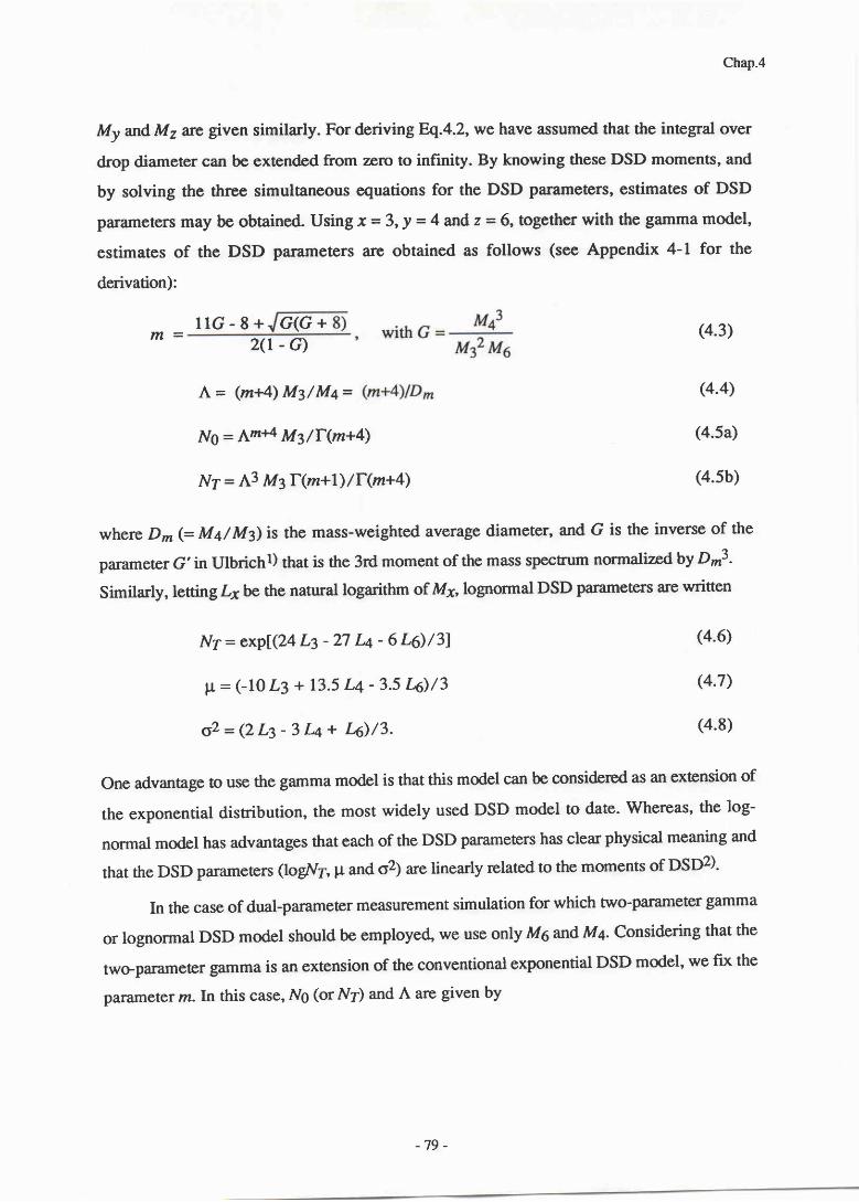
Chap.4
My and Ms are given similarly. For deriving W.4.2, we have assumed that the integral over
drop diameter can be extended from zorct to infinity. By knowing these DSD moments, and
by solving the three simultaneous equations for the DSD parameters, estimates of DSD
parilmeters may be obtained. Usingx=3,! =4 and z=6, together with the gammamodel,
estimates of the DSD parameters are obtained as follows (see Appendix 4- 1 for the
derivation):
″ =HG-8+
2 ( 1 - G )
A=(″ ■4)″ 3/M4=
(4。3)
(4.4)
(4.5a)
(4。5b)
(4.6)
(4。7)
(4.8)
where D″(=″4/″3)iS the mass―weighted average diameter,and C is the inverse of the
parameter G′in Ulbrichl)thatis dle 3rd moment ofthe mass specmm nomalized by D“3.
simuarly,lcttlng Lx be the natura1loganthm ofЛ々,bgnOllllal DSD pararrleters are―tten
ハb=A″ ■4ルf3/「02+4)
Ⅳr=A3″ 3「(″+1)/F(″+4)
Nr=CXp[(24L3-27L4-6L6)/3]
μ=(-10L3+13.5L4-3◆ 5L6)/3
σ2=(2L3-3L4+J%)/3.
One advantage to use the gamma model is that this model can be considered as an extension of
the exponential distribution, the most widely used DSD model to date. Whereas, the log-
normal model has advantages that each of the DSD parameters has clear physical meaning and
that the DSD parameters (1ogN6 p and &) arelinearly related to the moments of DSD2)-
In the case of dual-parameter measurement simulation for which two-parameter gamma
or lognormat DSD model should be employed, we use only M6 and Mq. Considering that the
two-paramercr gamma is an extension of the conventional exponential DSD model, we fix the
par:rmeter m.In this case, Ng (orNf) and A are given by
G(G+
-79-

Similarly, we fix o for the lognormal model according to Feingold and Irvin2). In this case,
Nl and p are given by
Nr = exp(3k - 2k + 12 o2)
v= (k - L4 - LO &)/2.
A=[(″ +5)(″+6)M4/M6]1/2
NO=A″ +5M4/「 (″+5)
Ⅳr=M4A4「 (燿+1)/Fレ:+5).
m=0 2O:24 JST March 9, 1980$min Average,Rain rate =2.24 mrnlh
O Measured data2-parameter model- Gamm? (m = 0. fixed)- Ganuna (m = 8, fxed)
$pararneter model- - Gamma
(Estimated m= -.84)---- Lognormal
(Estimated o = 0.50)ヽ。
m=8
∞ :08JST May18,1981
3‐min Average,
Rain rate=1.91 mnVh
o Measured data
2‐parameter modd― G a r n m a ( m = 0 , 徹呵――一 Garnma(m=8,1鴻 o
3parameter mode:一 ― G a r n I T l a
(Estimated m■29。1)
――――Lognormal
(Egmated σ=0■η
′F
l
9
針
I
=
Chap.4
“.9)
(4.10a)
(4.10b)
( 4 . 1 1 )
(4.12)
As mentioned above, the DSD parameters derived by this methd are similar to those to be
estimated through the dual-parameter radar measurement combining radar reflectiviry and
microwave or millimeter wave attenuations.
Examples of the model fitting of disdrometer-measured DSD are shown in Figure 4- 1-
1。41。
4
1♂ 1。3
1♂
(?ETEE)(∩)Z
ご。ETEE)(口)Z
101 1(ゞ
1む1 2~ 聡 4
1む1 2 3 4
Diameter(mm)Diameter (mm)
Figure 4-1. Examples of model fitting of measured DSD with the higher-order moment estimation.
‐80-

Chap.4
The right example shows the result for very large m and very small o, while the left one
shows small (negative) m and large o. It is found that the three paftlmeter models are flexible
enough to fit these two extreme DSDs very well. On the other hand, the two-parameter
models do not seem to work well for the wide variability in DSD shape. As shown later,
however, the two-parameter models can be used fine at least to estimate other IRPs the
kernels of which are not different much from those of the measurables.
4.2 Statistics of DSD Parameters
Figures 4-2 to 4-4 show the histograms of the exponential, gamma and lognormal
model parameters, respectively, as derived from Eqs.4.3-4.5 for the disdrometer data over
the two years. Note that the logarithms of the DSD parameters have been used to make the
histograms for N0, Nr and A. In Figure 4-5, the cumulative distribution of Ng of the
exponential model for the data having rain rates higher than 3 mm/h is plotted on a normal
distribution scale, showing that Ng is approximately log-normally distributed. The histogram
of N9 in Figure 4-2 has some skewness, which is caused by the DSD variation at light rain
rates. Similar properties have been observed for the Nr s of the gamma and lognormal
models. Roughty speaking, it can be said that the pdf s of Ng (gamma model, with m = O-3
fixed), Nr's, and A are approximately log-normal. The same is true for log(n+4) as sug-
gested by Eq.4.4. Major statistical quantities of those DSD parameters are listed in Tab1e 4-1-
One of the interest in the DSD modeling with the gamma distribution is the values of z
naturally found. It is shown that the values are clearly larger than zero (exponential distribu-
tion) and are somerimes very large (> 20). It should be noted that the mvalue is obtained from
the higher order moments and may not represent the DSD shape at small to intermediate drop
diameter region. As indicated from Eq.4.3, m can be extremely large as the parameter G
approaches unity. Since G is determined by a relative magnitude amon g M3, Ma and M6, itis
expected that only a small DSD change causes a large variation rn m when the DSD has a
niurow standard deviation and therefore that such a large change in m is not significant in
fitting the DSD. For comparison, we have derived rn values from lower-order moments (e.g.
Mg, Ml and MZ) and have found that they are somewhat smaller and more stable than the m
value derived from M6,M4andM3.This means that apart of the variation in rn comes from
natural and/or sampling fluctuations of DSD at larger drops. Later in this chapter, more
discussion is made on the mvalue relating to the accuracy in rain rate estimation-
‐81

Chap.4
“Cコ00
. 5 . 6 . 7
Logls A
Figurc 4-Z ttiSqram of exporrcltial DSD modcl pilartct€ns.
-82 -
Chap`
〓
コo0
14
1
1
1“Cコ00
m
一Cコ00
Fu“ 4‐3. Histo_ofgamm DSD moel“ 副鵬曖 .
‐83‐

Chp.4
1
14
12
=1コ0
0
1
14
1
を1
コ0 ・
0600
400
200
.1 .12 .14 .16 。 18 .2 .22 .24
σ2
Figgre 4-4. HistOgram of tognorrnal DSD model parargcrs.
.06.04 .26
‐8 4 ‐
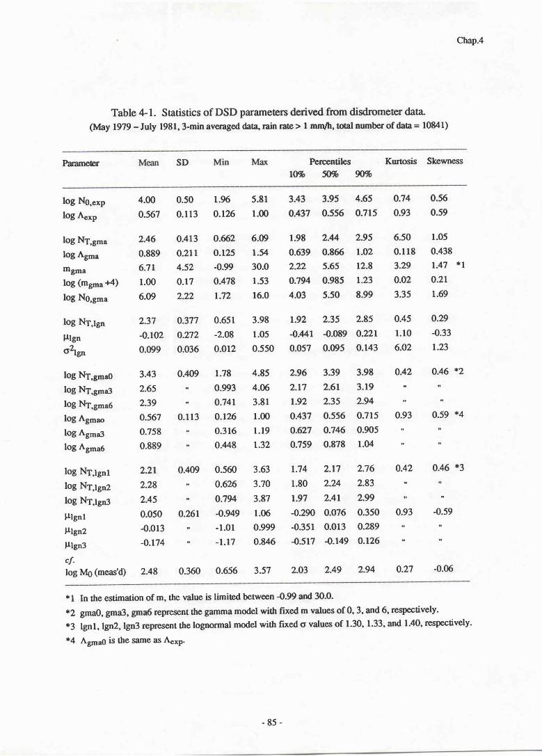
Chap.4
Table 4-1。Statistics of DSD paramecrs derived k)m disdrometer daほ
( M a y 1 9 7 9~J u l y 1 9 8 1 , 3 - m i n a v e r a g e d d a t r a i n F a t e > l m m , t O t a l n u m b e r o f d a鯰= 1 0 8 4 1 )
P a r a m e t e r SD Percentiles Kurtosis Skewness
10% 50m 90%
log NO,exp
l o g A e x p
l o g N Tっgma
l o g A g m a
mgma
10g(mgma■ 4)
log NO,gma
log NT,lgn
μlgn
σttgn
bg NT,gma0
log NT,gma3
log NTっgma6
log Agmao
log Agma3
log Agma6
log NT,lgnl
log NT,lgn2
log NT,lgn3
μlgnl
μlg■2
μlgn3
手
log MO(meas'の
4。00 0.50
0.567 0.113
2.46 0。 413
0.889 0.211
6.71 4.52
1.00 0。 17
6.09 2.22
2.37 0.377
‐0.102 0.272
0。099 0.036
3.43 0。 409
2.65 ・ ・
2.39 "
0.567 0。 113
0.758 '=
0.889 '1
2.21 0.409
2.28 ・ ・
2.45 "
0。050 0.261
-0。013 "
-0。174 ・・
2.48 0.360
1.96 5。 81
0。126 1。 00
0.662 6.09
0。125 1.54
-0.99 30。 0
0.478 1.53
1.72 16.0
0。651 3.98
‐2.08 1.05
0.012 0.550
1.78 4。 85
0.993 4。 06
0。741 3.81
0.126 1.00
0.316 1.19
0.448 1.32
0.560 3.63
0.626 3.70
0.794 3.87
-0。949 1.06
‐1.01 0。999
-1.17 0.846
0。656 3.57
3.43 3。95 4.65 0.74
0437 0.556 0.715 0。 93
1.98 2.44
0.639 0。 866
2.22 5.65
0。794 0.985
4.03 5.50
2.95 6.50
1.02 0.118
12.8 3.29
1.23 0.02
8.99 3.35
0.56
0.59
1.05
0.438
1.47 *1
0.21
1.69
0.29
-0.33
1.23
0.46 *2
0.59 *4
0.46 *3
-0.59
‐0.06
1.92 2.35 2.85 0。 45
-041 -0.089 0.221 1.10
0。057 0.095 0.143 6.02
2.96 3.39 3.98 0.42
2.17 2.61 3.19 ・ ・
1.92 2.35 2.94 ・ ・
0.437 0。 556 0。 715 0.93
0.627 0。 746 0。 905 =1
0.759 0.878 1.04 。 1
1.74 2.17 2.76 0。 42
1.80 2.24 2.83 "
1.97 2.41 2.99 。 '
-0.290 0。 076 0。 350 0.93
-0.351 0。013 0.289 1'
-0.517 -0.149 0.126 ・ ・
2.03 2.49 2.94 0.27
*l ln the estimation of m,the valuc is limited betw∝n-0."and 30.0.
*2 gmaO,gma3,gma6 representthe gamma model widl rlxed m valucs of O,3,and 6,respctively.
*3 1gnl,lgn2,lgn3 represclltthe 10gnomal modd with rlxed σ values of l.30,1.33,and l.40,respecivdy.
*4 AgmaO is dle same as AcxP.
‐85‐

Chap.4
90
刀
∞
30
10
{メ}ン一一一一o一0』LΦ>コ0「Eコ0
99。99
99.9
99
0。1
0。01
May 1979 ru July 1981
Rain rate:3 ru &4 mm/h
3+nin averags
Number of data: 2996
Mean: 4 .10
o = 0.4if6
3。0 4.0 5。 0
Log NO{mm~lm~3}
Figrre 4-5. Cumulative distribution of Ng of the exponential DSD model.
4.3 fnterrelations among DSD Parameters and DSD Moments
4.3.1 Rain rate and Z factor dependences of DSD parameters
There has been a wide range of interest in the problem how DSD parameters change
with rain rate, the most widely used rain parameter. This is because the knowledge of such
relationships is useful to estimate various IRP relations such as Z-R relation, and to model
DSD's at other locations where only rain rate data are available. Similarly, the Z factor
dependence would be useful to make a modeling of DSD in radar measurements in which Z
factor profile is a primary oulput.
‐86-

Chap.4
Figures 4-6 to 4-8 show respectively the rain rate dependences of the exponential,
gamma, and lognormal model parameters. The large variabilities in these DSD parameters are
also clear in these figures. It is also found that the variability is generally larger in light (*3
mm/h) to moderate (3 - 15 mm/h) rain rates; at heavy rain rates (5 15 mmlh), the DSD
parameters are much less variable. This suggests that physical processes producing healy rain
rates at Kashima are relatively similar. On the other hand, light to moderate rain rates should
be generated from various precipitation processes which result in the large variation in DSD.
Similar properties have also been obtained for the relations between the DSD parameters and
Z. From those results, the following conclusions are drawn (subscripts "exp", "gma" and
"lgn" represent the values for the exponential, gamma and lognormal models, respectively):
(1) A"*p and Agma &ro clearly dependent on R andZ.
(2) No.*o has only a small and little dependences on R and Z, respectively.
(3) Nr"*p, Nrg*" and Nrtgn have similar properties to Ng"*p but for somewhat larger
dependences on R andZ.
(a) The parirmeter m has smallR and Zdependences, indicating thatDSD is somewhat more
concave-down at heavy rain rates than light rain rates, although the variability of rh at light
rain rates is very large.
1.
6
5 . 5
5
1.4
1 .
oZ
o,00J
.5 1 1.5
Logl。 Of Rain rate
. 5 1 1 . 5Logro of Rain rate
Figure 46. Rain rate dependences of the exponential DSD parameters, May 1979 - July 1981.
曲露F彗
°4
3.5
3
2.54こ
2・r e
. 4
t
。2f 。
‐87‐

0 ‐ F 』 C 一 卜 Z 一 。 O r ● q 】
30 2 20 1
E
T l.6
El・4
c l.2
< 1
0 0 。
0 」°
10 5 0
‐5
。5 1 1.5
Log1 0 0f rain rate
Figure 4‐7。
0 .5 1 1.5 2
Log1 0 0f rain rate
o .5 1 1.5
Log1 0 of rain rate
Rai
n rat
e dep
ende
nces
of
the g
amm
a DS
D m
odel
para
met
ers,
M
ay 1
979 -
Jul
y 19
81.
‐ ∞ ∞ ‐2
1.5 1
=1 0
0.5
●1
・1.5
・2
2o
.si1
.s2
Lo
grO
of R
ain
rate
0
.5
1
'r.r
Lo
gro
of R
ain
rate
ヽ。2 。
2
●1 。
1
.05
.5
1
1.5
Lo
gro
of R
ain
rate
Fig
ure
4-8
.O F ” 「 ・ヽ
Rai
n rat
e dep
ende
nces
of
the l
ogno
rmat
DS
D m
odel
pam
met
ers,
M
ay 1
979 -
Jul
y 19
81.
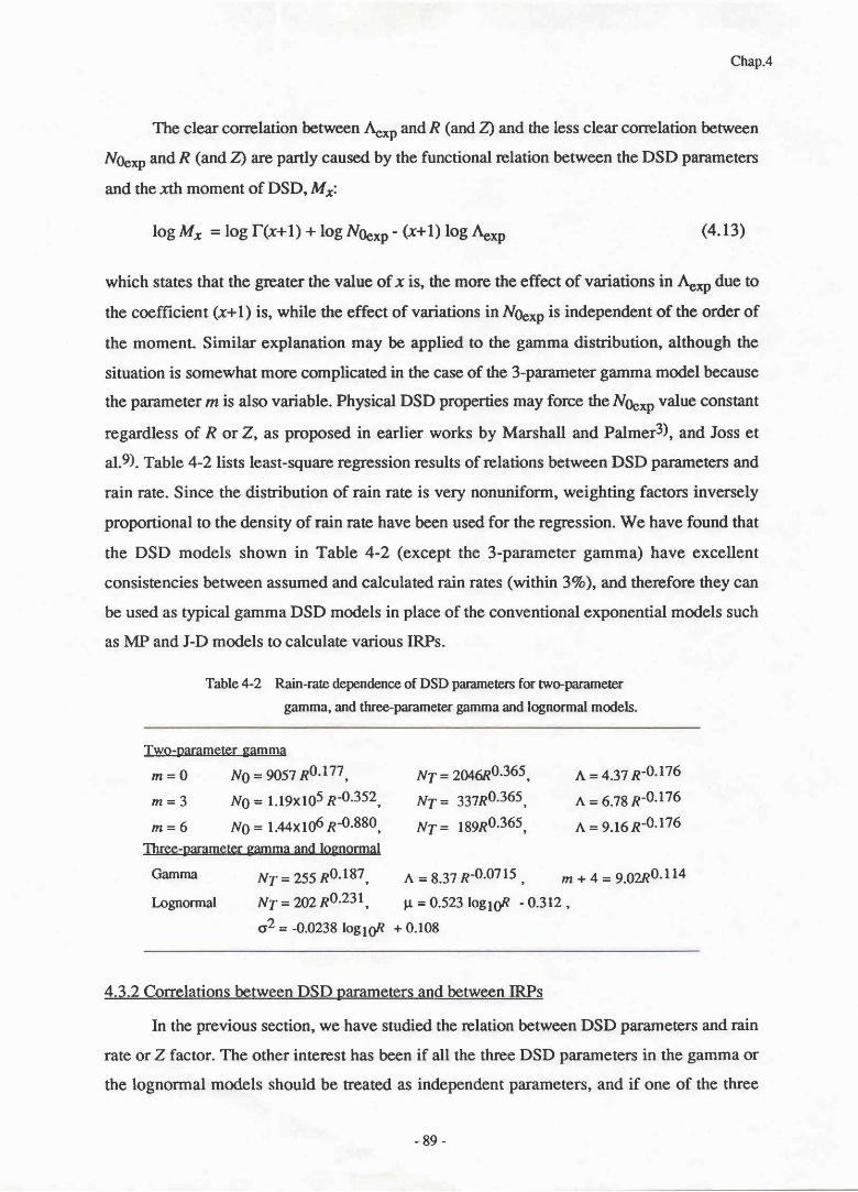
Chap.4
The clear correlation between &*p and R (and 4 arrd the less clear correlation between
Nge*p and R (and 4 ue partly caused by the functional relation between the DSD parameters
and the xth moment of DSD, Mr:
log M, - log f(x+l) + log Ng"*p - (x+1) log &*p ( 4 . 1 3 )
which states that the grcater the value of x is, the more the effect of variations in 4*p due to
the coefficient (-r+1) is, while the effect of variations in Ng"*o is independent of the order of
the moment. Similar explanation may be applied to the gamma distribution, although the
situation is somewhat more complicated in the case of the 3-parameter gamma model because
the parameter m is also variable. Physical DSD properties may force the N66*n value constant
regardless of R or Z, as proposed in earlier works by Marshall and Palmer3), and Joss et
al.9). Table 4-2 lists least-square regression results of rclations between DSD parameters and
rain rate. Since the distribution of rain rate is very nonuniform, weighting factors inversely
proportional to the density of rain rate have been used for the regression. We have found that
the DSD models shown in Table 4-2 (except the 3-parameter gamma) have excellent
consistencies between assumed and calculated rain rates (within 3Vo), and therefore they can
be used as typical gamma DSD models in place of the conventional exponential models such
as MP and J-D models to calculate various IRPs.
Table4-2 Rain-rate dependence of DSD pammeters for two-parameter
gamma, and three-parameter gamma and lognormal models.
Two-oarameter gamma
m = O N0 = 9057 P0'177 ,
m=3 N0= l . l 9x1g5P-0 '352 ,
m=6 N0 = 1.44x10⁶P-0.880,Three-parameter gamma and lognormal
Ⅳr= 2 0 4“ 1 0。3 6 5 ,
Ⅳr〓 3 3 7 R O・3 6 5 ,
N r = 1 8 9 R O・ 3 6 5 ,
A=4.37R~0・ 176
A=6.78R~0。 176
Λ =9。16R~0。176
Gamma
I-ognormal
ⅣT= 2 5 5 R O・1 8 7 , A = 8。 3 7 R…0・0 7 1 5 , “ + 4 = 9。 0 2 R O・1 1 4
1Vr=20220・ 231, μ =0.523 1og10R ~0・ 312,
σ2=_0.0238 1og10R +0・ 108
4.3.2 Correlations between DSD parameters and between IRPs
In the previous section, we have sfudied the relation between DSD parameters and rain
rate or Z factor. The other interest has been if all the three DSD parameters in the gamma or
the lognormal models should be treated as independent parameters, and if one of the three
‐89-
Chap.4
parirmeters can be fixed or not. It should be noted that answers to these questions generally
depend on the combination of IRPs to be employed to derive the DSD parameters. For
example, if all IRPs of interest a.re only higher order moments, simple two-parameter models
(e.g. exponential model) may be enough because the DSD modeling need not take care of the
variation in DSD at small drop diameters, enabling the modeling much simpler. Figure 4-9
shows the correlations between m and logNg and between m and log A for the gamma
distribution. As shown in these figures, there are high correlations between m and other
parameters. The existence of the Ng-z relation was suggested by Ulbrichl) to reduce the
three-parameter gamma to the two-parameter gitmma distribution; however, it has also been
pointed out that such a relation could come from a statistical correlation between DSD
parameters rather than due to physical DSD propertiesl0). The /v-m relation is also due to a
statistical correlation between A arrd m, and expected from W.4.4 which states that A is given
by the product of m+4 andD*-1. Since D^is fairly stable, the large variation inm as seen in
Figures 4-3 and 4-7 is directly reflected to the variation in A. These correlations are also
recognized as a "compensation" effect to give reasonable IRP values. On the other hand, there
are little correlation between N7 and A andNl andm, as shown in Figure 4-10. This may be
due to the fact that the total drop concentration, N1, follows the Poison distribution and
independent of the physical processes producing the "shape" of DSD and determine the other
DSD parameters, A and m. For this reason, Chandrasekar and Bringito) recommend the use
of N1 rather than Ng as one of the gamma DSD parameters.
It is not clear at present that the relationships shown above are useful to reduce the
three parameter DSD model to a two-parameter model because the high correlations are
essentially caused by the large variation inm. Considering that the large mvalue is caused by
a minor fluctuation in G (see Eq.a.3) and it is not so essential to fit the natural DSD
reasonably, we can restrict the m value within a range between 0 to 8, for example. In such
case, correlations in the Ng-m relation and the lv-m relation are not high as can be seen from
Figure 4-9. More study is needed on the problem how the gamma DSD parameters should be
defined and on the same problem for the lognormal model.
Later in this chapter, we will test more straightforward scheme to reduce the three
parameter DSD model to a two-parameter model; to fix one of the three DSD parameters as
has been tried by many researchers.
- 9 0 -

18
y=0.404x+3.390r=0.79
Chap.4
.8 1 1.2 1.4 1.6 1.8
Log10(mt4)
1
く
0”OOコ
oZ
o,00コ
14
12
10
8
6
4
2
0
2
1 . 8
1 .
1.4
1 0 1 5 2 0 2 5 3 0
m
Figure 4-9. scauergrams of the gamma DsD model panmeters;m vs. log /Vg and log (m.tA) vs. log A.
3
2
くo l . 2
ヨ 1. 8
. 6
. 4
. 2
0
2
15
10
5
0 ■β8_、、.
3 4Logle N1
Figure 4-10. scattergrams of the gamma DsD model pararneters;log N1 vs. log A and log N1 vs. tn.
y=1.08x‐ 0.183,r=0.85
‐91-

Chap.4
4.3.3 Relations between IRps
A. Correlation between two dffirent nnments
Because of the fluctuation in DSD, the relationship benveen different moments changesfrom time to time. Figure 4-Il shows scattergrams of rain rate versus several momentsranging from Mgto M6-Itis clearly shown that the correlation becomes low when the orderof the moment departs from that for rain rate (= 3.67). Chandrasekar and Bringil0) derivedthe correlation coefficient between Mrand, Mr, r*, in the case where DSD fluctuation issolely due to statistical sampling error:
r(m+x+y-b+ I )r -, ry (4.14)
r (m+2x - b +I)UZ y 12a2y - b + DUz
where lzl is the gamma DSD parameter, and b (= 0.67) is the exponent of a power_law relationbetween the terminal velocity of raindrops versus drop diameter (Eq.2.12). For derivingEq'4'14, tt is assumed that the DSD follows a gamma distribution, that total number ofraindrops follows Poisson distribution, that sampling volume (for a given diameter range) isproportional to the terminal velocity (8q.2.12), and that realizations of DSD are independenrand identically distributedl 0).
It should be noted that rry's between higher-order moments are fairly high even whenonly statistical DSD fluctuations exist (see Fig.4-12). Thus, we should be careful ininterpreting IRP relationships derived from DSD data with a small sampling volume (or shortintegration time) in which the sampling error can be a dominant cause of DSD variation. Asdiscussed in 3.1.2, however, the sampling fluctuation (for Poisson process) in the 3-minaveraged disdrometer data is relatively minor, and therefore the data should well representphysical DSD variations as well as the sampling fluctuation regard.ing the gamma pdf (if any).
Correlation analyses are made of the moments calculated from disdrometer data. Theresultant correlation coefficients are then compared with the value calculated with Eq.4.14. Toinvestigate short-term and long-terrn DSD fluctuations, three kinds of time segments havebeen used; short-term (0.5 - 1.5 hours within arain event), intermediate term (several days)and long-terrn (several months). The results obtained from each time segment are thenaveraged, and plotted on Figure 4-12 as well as the theoretical curve (Eq.4.14). It is foundthat in general the correlation coefficients obtained from the disdrometer data are higher thanthe theoretical results assuming reasonable rn values of 0 - 8, especially for short-term
- 9 2 -
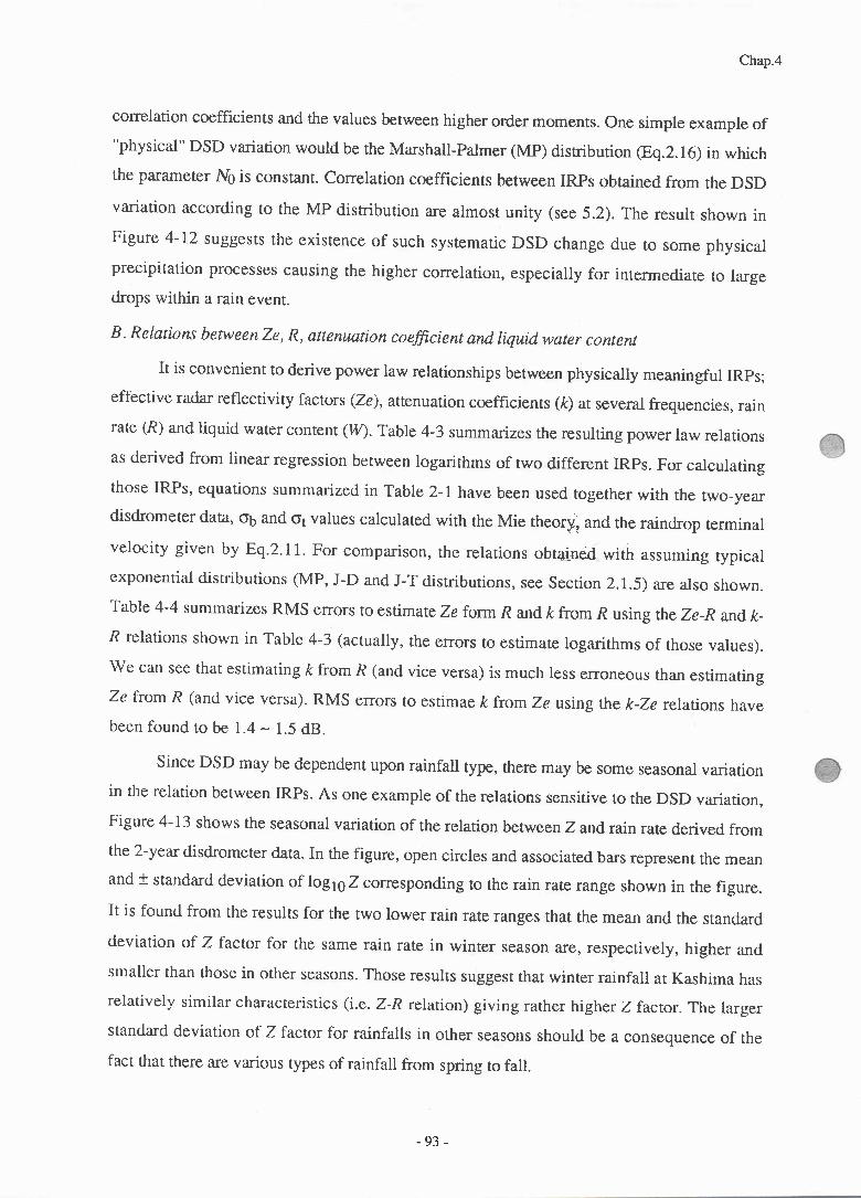
Chap.4
correlation coefficients and the values between higher order moments. One simple example of"physical" DSD variation would be the Marshall-Palmer (MP) distribution @q.2.16) in whichthe parameter Ng is constant. correlation coefficients between IRPs obtained. from the DSD
variation according to the MP distribution are almost unity (see 5.2). The result shown inFigure 4-I2 suggests the existence of such systematic DSD change due to some physicalprecipitation processes causing the higher correlation, especially for intermediate to largedrops within a rain event.
B . Relations between Ze, R, attenuation cofficient and liquid water content
It is convenient to derive power law relationships between physically meaningful IRps;effective radar reflectivity factors (Ze), attenuation coefficients (&) at several frequencies, rainrate (R) and liquid water content (W. Table 4-3 summarizes the resulting power law relationsas derived from linear regression between logarithms of two different IRps. For calculatingthose IRPs, equations summarized in Table 2- t have been used together with the two-yeardisdrometer data, 06 and 01 vslues calculated with the Mie theory, and the raindrop terminalvelocity given by Eq.2. r 1. For comparison, the relations obtained witir assuming typicalexponential distributions (MP, J-D and J-T distributions, see Section2.l.5) are also shown.Table 4-4 summarizes RMS elrors to estimateZe form R and k from R using theZe-Rand ft-R relations shown in Table 4-3 (actually, the errors to estimate logarithms of those values).We can see that estimating k from R (and vice versa) is much less erroneous than estimatingZe fromR (and vice versa). RMS errors to estimae kfrom Ze usingthe k-Ze relations havebeen found to be 1.4 - 1.5 dB.
Since DSD may be dependent upon rainfall type, there may be some seasonal variationin the relation between IRPs. As one example of the relations sensitive to the DSD variation,Figure 4-L3 shows the seasonal variation of the relation betw een Z and rain rate derived fromthe 2-year disdrometer data. In the figure, open circles and associated bars represent the meanand * standard deviation of logto Z corresponding to the rain rate range shown in the figure.It is found from the results for the two lower rain rate ranges that the mean and. the standarddeviation of Z factor for the same rain rate in winter season are, respectively, higher and.smaller than those in other seasons. Those results suggest that winter rainfall at Kashima hasrelatively similar characteristics (i.e. Z-R relation) giving rarher higher Z factor. The largerstandard deviation of Z factor for rainfalls in other seasons should be a consequence of thefact that there are various types of rainfall from spring to fall.
-93-
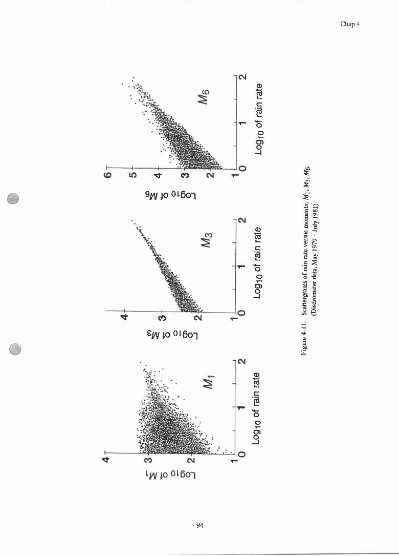
4 3
● ミ ち 。 5 3
3 2
一 ミ b o r o o J, つ ヽ ‐
1L
og
rO of r
ain
rate
1
Log10 0f rain rate
Fig
ure
4-ll.
sc
atte
rgra
ms o
f ra
in ra
te v
ersu
s mom
ents
; M1,
M3,
M6.
(Dis
dro
me
ter d
ata
,Ma
y 1
97
9 -
July
lgg
l)
1L
og
tg of r
ain
rate
0 , ” や ヽ

瀑ヽ ミ MO vs. moments―卜、=ト
一
一
一
‐・・ヽ
、 、ヽ、し、ヽ
一 mゝ
n イ
コ
ゝ 卜、、
∠ l=2
\
ヽ\
ヽ
・・・・・
\ ゝ :\ ヽ
「ヽヽ ヽ
Chap.4
o Shortterm ^ Intermediateterm r Lorgternr
1 1 . 5 2 2 . 5 3 3 . 5 4 4 . 5 5
0rder of moment correlated wnh M。
1 1 . 5 2 2 . 5 3 3 . 5 4 4 . 5 5Order of moment correlated with Mg
1 1 . 5 2 2 . 5 3 3 . 5 4 4 . 5 5
C)rder of rnoment cOrrelated with M6
Figllre 4-12。COrreladon cOefficients between mOments Of DSD;dleoredcal calculation(curVes)
and alose obtained hm disdrometer data for several temporal scales.
一EΦ一0一〓000)CO〓“一Φ」」00
一cΦ一OLの00
c〇一t
3
ヒOO
‐95‐
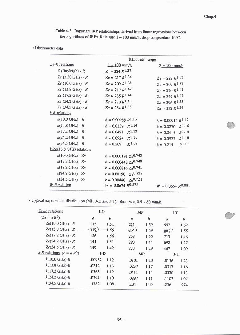
Chap.4
Table 4-3. Important IRP relationships derived from linear regressions betweenthe logarithms of IRPs. Rain rate I - 100 mm/h, drop temperature lgoC.
. Disdrometer data
盈 ―R r e h t i o n s
Z OLayleigh)―R
ル (5。30 GHz)― R
ル (10.O GHz)_R
ル (13.8 GHz)‐R
ル (17.2 GHz)‐沢
ル (24.2 GHz)‐R
ル (34.5 GHz) R̈
た収 r e l a t t o n s
た(10.O GHz)‐R
た(13.8 GHz)―R
た(17.2 GHz)‐R
た(24.2 GHz)¨R
た(34.5 GHz)‐R
l-2(13.8GHハ Кladons
た(10.O GHz)‐Z`
た(13.8 GHz)―Z`
た(17.2 GHz)‐Z`
た(24.2 GHz)‐Z`
た(34.5 GHz)‐Z`
W―R relation
Rain rate range
l~ 1 0 0 m m / h
Z = 2 2 4 R l・ 3 7
Z ` = 2 1 7 R l・3 6
Z ` = 2 0 9沢 1・3 8
Z ` = 2 1 7 R l・4 2
Z ` = 2 3 5 R l・“
Z ` = 2 7 0 R l・4 3
Z ` = 2 8 4 R l・3 3
た= 0。∞ 9 8 8 R l・1 3
た=0.0239 Rl・ 14
た=0.0421 Rl・ 13
た=0.0924 Rl・ 11
た=0.209 Rl・ 08
た=0.000191 ZeO・ 743 ~
た=0.000448 ZeO・ 748
た=0.000816 ZeO。 741
た=0.00190 zン 0。728
た=0.00440 Zセ 0。721
7 = 0。 0 6 7 4 R O・8 7 2
3~ 100 mm/h
Z ` = 2 2 7 R l・3 3
Z ` = 2 0 9 R l・3 7
Z ` = 2 2 0 R l・4 1
Z ` = 2 4 4 R l・4 2
Z`=296 Rl・ 38
Z ` = 3 3 2 R l・2 4
た= 0 . 0 0 9 1 4 R l・1 7
た=0.0230 Rl・ 16
た=0.0415 Rl・ 14
た=0.0927 Rl・ 10
た=0.215 Rl・ 06
7 = 0 . 0 6 6 4 R O。8 8 1
' Typical exponenr.ial distribution (Mp, J-D and J-T). Rain rate, 0.5 - g0 mm/h.
Ze-R relations
(Ze = a Rb)
Ze(rO.O GHz) - R
Ze(r3.8 cHz) -,n
Ze(17.2 cHz) - RZe(24.2 cHz) - RZe(34.5 GHz) - R
t-R relations (k -- a Rb)
t(10.0 GHz)-Rft(13.8 cHz)-Rk(rl .2 GHz)-Rk(24.2 cHz)-Rk(34.5 GHz)-R
J―D
α
l15
-112♪
126
141
149
J‐D
.00952
.0212
.0363
.0794
。1782
MP
α
211
、三
∋
258
290
270
MP
,0101
.0237
. 0 4 1 1
.0897
.204
J.T
a b
557 r.62
Aqr) r.ss7r3 r.46692 r.27467 1.09
J-T.0136 r .23.0317 1.16.0530 1.13.r 103 r .07.236 .974
b
1.51
1.55
1.56
1.51
1.42
1 . 1 2
1 . 1 3
1 . 1 2
1 . 1 0
1.08
b
1.59
1.59
1.55
1.44
1.29
1.20
1 . 1 7
1 . 1 4
1 . 1 1
1.05
‐96-

Chap.4
Table 4-4. RMS dB errors to estimate Z fromR, and & from R using the IRP relations shown in Table 4-3.(disdrometer dara, R = I - 100 mm/h, May 1979 -rJuly lggl).
Estilnatingた
た(10.OGH⇒
た(13.8 GHz)
た(17.3 GHz)
た(24.2 GHz)
た(34.5 GH2)
Esdmadng盈
ル ( 5 . 3 G ]財
ル (10。O G H 2 )
2 ( 1 3 . 8 G I・I z )
2(17.3 GHz)
ル (24.2GL)
2(34.5 GHz)
0。88 dB
O。91 dB
O.83 dB
O.67 dB
O . 5 4 d B
2 . 4 d B
2 . 5 d B
2 . 8 d B
2。9 d B
2 . 9 d B
2 . 5 d B
4
53
(ШN N〓0‥い.い) 00コ
…………………………………‐-200R106
――'200Rl.6
10-16 MM/H
O
1979 1980
YEAR′ MONTH
1981
Figure 4-13. Seasonal variation in the relation between Zfacnrand rain ratederived frrom the 2-yea disdrometer daa.
F,ヽ 」
一―一
―
一
ヽ
一
―一十一 一
一
6
H
・
3
5
/
1
・
,M
6
R
6
2
M
o
O
¨
H
¨
1
0
6
/
6
R
2
1M
・
0
′ 一 μ 「|。(
′.、,ごl.:ノ|97
(
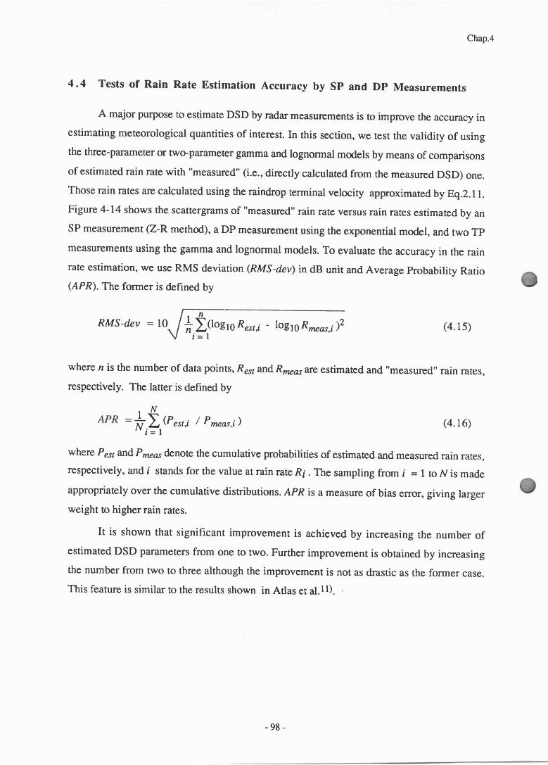
Chap.4
4.4 Tests of Rain Rate Estimation Accuracy by SP and DP Measurements
A major pu{pose to estimate DSD by radar measurements is to improve the accuracy inestimating meteorological quantities of interest. In this section, we test the validity of usingthe three-parameter or two-parameter gamma and lognormal models by means of comparisons
of estimated rain rate with "measured" (i.e., directly calculated from the measured DSD) one.Those rain rates are calculated using the raindrop terminal velocity approximated by Eq.2.l l.
Figure 4-14 shows the scattergrams of "measured" rain rate versus rain rates estimated by an
SP measurement (Z-R method), a DP measurement using the exponential model, and two Tp
measurements using the gamma and lognormal models. To evaluate the accuracy in the rainrate estimation, we use RMS deviation (RMS-dev) in dB unit and Average Probability Ratio(APR). The former is defined by
(4. 1s)
where n is the number of data points, Rs5s and R*o, are estimated and "measured" rain rates,
respectively. The latter is defined by
/ P^rorJ) (4. 16)
where Prrl and P*r^ denote the cumulative probabilities of estimated and measured rain rates,respectively, and i stands for the value at rain rate Rg . The sampling from i = I to N is made
appropriately over the cumulative disrributions. APR is a measure of bias error, giving larger
weight to higher rain rates.
It is shown that significant improvement is achieved by increasing the number of
estimated DSD parameters from one to two. Further improvement is obtained by increasing
the number from two to three although the improvement is not as d.rastic as the former case.
This feature is similar to the results shown in Atlas er aI.11).
R盗‐ね=1/ヽti10gЮR鉗F_bgЮ R″αJメ
PNマん〓‐
1一Mュ
〓
- 9 8 -
Chap.4
Z‐R rnethod (z=200 Rl・ 6)
r =0.888
RMS― dev=1.6 dB
APR=0。 703
=ヽ
EEC
O
“L
C
“L
0①
C
E一
∽①
0
0
00」
2.5
2.0
0 . 5
0 . 0
2 . 5
2 . 0
1 . 5
1 . 0
0。5
0. 0
1.5
1.0
Gamma DSD model Lognormal DSD model
0.0 0.5 1.o
Logl。 Of
1.5 2.0 2.56
r= 1。 ooo
RMS― dev=ooo2 dB
APR=1。 003
イ
′′
r = 1.ooo
RMS― dev=0。 03 dB
APR=1。 013
1.5 2。 0 2.5
in mm/h"measured" rain rate
Figure 4-14. Comparison of rain rate estimates by an Sp measuement (Z-R method),a DP measurement using the exponential DSD model, and nvo Tp measurcmensusing the gamma and lognormal DSD models.
Exponential DSD model
r=o.999
RMS‐ dev=o.13 dB
APR=1。 057
‐99‐

Chap.4
For reducing the number of independent DSD parameters, it has been common to fixone of the parameters, specifically m for gammal2-14) and o for lognormal mode1r2,l5).
Dependence of rain rate estimation accuracy on m or on o is examined by a simulation of Dp
measurements using M4 and M6.The results, which Eue summ arrzed,in Figure 4-IS,indicate
thatm from 6 to 8 and o from 0.28 to0.29 give the lowest RMS and bias errors, although theaccuracy is not very sensitive to the shift in m and o. The similarity in the kernel between kand R probably contributes to this insensitivity, because a comparison of rain rate estimatesdeduced from various combinations of moments, (Mg,M6),WZMA), etc., has indicated that
the estimation accuracy becomes more sensitive to the choice of m when the kernel of themoment combined with M6becomes far from that for rain rate (= 3.67).
1。06
1。04
Gamma model with fixed m0.3
20■1.
匡Lく
(mこ>Φマ∽〓匡
2
1
0
0
(mこ>Φマ∽〓匡
1
5
0。
o0
1。0
.9Ъ0
1。02
襲1・0
。98
m
;--O(t't'-
・― ← ・一 ・́`
RMS‐ dev
.24 .26 .28 .30σ
8 10
。34 覇0
Figure 4-15. Dependence of rain rate estimation accuracy on the gamma DSD parameter mand on the lognormal DSD parameter o.
-100-
Chap.4
- Discussion on the "best" m value
The best m and o values (in the sense that they provide the lowesr RMS deviation)
obtained here are somewhat different from the results of previous works using Z and Zon
combinations (m -Z - 512-14)' o = 0.34 t5) '). Although the accuracy remains excellent over
fairly wide ranges of m and o (see Figure 4-15), it may be worth making some comments on
the m and o values obtained here. We make comments only on the nz value since the same
discussion can be made just by noting that "large" mcorresponds to "small" (t.
We should note that the quantities of interest here are all higher order moments. As
mentioned earlier in this chapter, the use of lower-order moments for the DSD estimation does
lower the m estimate. This suggests that the DSD properties at large drop diameters contribute
to the large rn value rather than those at small drop diameters. Even so, it may be worth while
to check the effect of DSD at drop diameter less than about I mm where the Joss-Waldvogel
type disdrometer may have a degraded sensitivity because in many cases DSDs measured by
our disdrometer show a decrease in dtop density with diameter at the small diameter region
(see Chapter 3). For this pu{pose, we use the same test method described in Section 3.1; i.e.,
the disdrometer-measured DSD is artificially modified so that the DSD at less than 1 mm
diameter is exponentially distributed. The modified DSD is then used to derive rhe DSD
parameters. It is found that the exponentiation of the DSD at the small diameter region
approximately halves the m value when the original one is 6 to 8; i.e. the modined DSDs have
rn values of 3 to 4. However, it should also be noted that in general natural DSDs tend to have
a "concave-down" shape due to various raindrop evolution processesl) rather than the ex-
ponential shape assumed for the test. Thus, we may conclude that, if there is some instrument
sensitivity degradation at the small diameter region, the "best" rn value would be about 4 to 6.
The other aspect to be considered is the accuracy in estimating lower order moments.
As a limiting case, we test the zeroth moment estimation. The result, shown in Table 4-5,
indicates that the m=3 - 6 are best tominimize theRMS deviation, while m=6- 8 gives rhe
APR close to unity, and that the accuracy is much worse than that in the rain rate estimation.
Although there is some difference in the "best" m in terms of RMS deviation and APR, on
average, this conclusion is similar to that obtained in the rain rate estimation.
The definition of o in this thesis is different from that used in Feingold and Levinl5). Their "best" o of 1.4conesponds to o = 0.336 by our definition. (Letting their "o" be o" o = lno').
- 1 0 1 -
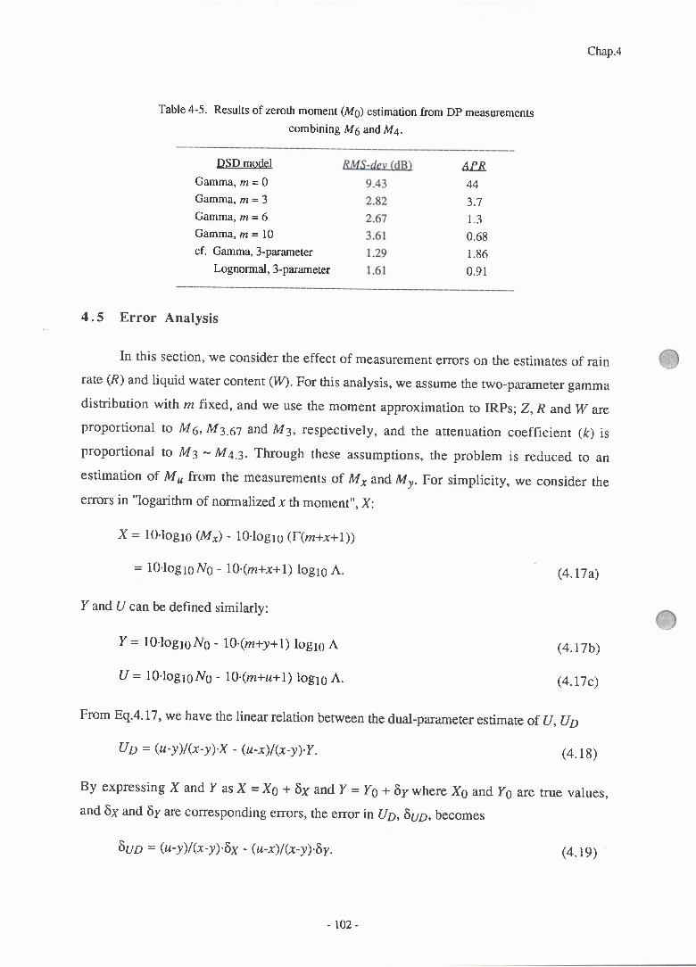
Chap.4
Table 4-5. Results of zerotlt moment (M9) estimation from DP measurements
combining M6 and M4.
D S D m o d e l
Gamma,“ =o
Gamma,″ =3
Gamma,″ =6
Gamma,“ =lo
cf.Gamma,3‐ parameter
Lognol‖lal,3‐pararneter
APR
44
3 . 7
1 . 3
0.68
1.86
0。91
4 .5 Error Analvsis
In this section, we consider the effect of measurement errors on the estimates of rainrate (R) and liquid water content (W. For this analysis, we assume the two-parameter gammadistribution with rn fixed, and we use the moment approximation to IRps; Z, R and,W areproportional to M6, Mz.ol and M3, respectively, and the attenuation coefficient (ft) isproportional to M3 - M43. Through these assumptions, the problem is reduced to anestimation of M , from the measurements of M, and, M r. For simplicity, we consider theerrors in "logarithm of normalized -r th moment", X:
X = l0.logro (M*) - tO.log1 s (t(m+x+l))
= 10.logt0N0 - 10.(m+x+1) loglg A.
IZ and U can be defined similarly:
(4。17a)
y=10・log10 ⅣO_lo。←ηtty+1)10g10A
υ=10。log10 NO_lo。(″+“+1)log10 A.
(4.17b)
(4.17c)
From Eq.4.17, we have the linearrelation between the dual-parameter estimate of (J,UD
びD=(“‐y)/α―y)・X―(“―χ)/α―y)。y.( 4 . 1 8 )
By expressing X and I as X -Xo + 6x and I' -Yg+ 6rwhere Xg and I/9 are true values,and 67g and 6y a.re corresponding errors, the error in (JD,6uD, becomes
6uo - @-y)l(x-y).6x - @-x)/(x-y).6r. g.D)
-102‐

Chap.4
Assuming that 6a and 6r are independent random variables with mean values of Ay and Ay
and standard deviations of oy and or, respectively, we have the mean and variance of 6y6r(Luo and oyp2, respectively):
△υD=(“ ‐y)/(χ―y)。△χ―(“―χ)/αずソ)・△y
σびD2=[(“_y)/∈ッ)]2.6x2+[(“_χ)/α―y)]2.σy2
(4.20)
(4.21)
(4.23)
(4.24)
It is clear from Eq.4.19 that the dual-parameter estimation becomes more accurarc withincreasing lx-yl; i.e., the orders of the two measurable moments should be apart from eachother in order not to amplify the measurement error. For comparison, a single-parameterestimate of u using x (Usx) and that using y (Usfl are derived:
USv - (v-u).(m+v+l)-lNO,Os + (r?r+ u+L).(m+v+l)-l X (4.22)
where V =X o rYandv=xo ry , andNg ,dB = l 0 . l og l0N0 .Le t t i ng t he mean and t hestandard deviation of the error in Ng,6g be Arrro and olgg, respectively, we have the mean(Ausv) and variance (ousvz) of the error in U5y , 6sy:
Lusv - (v-a).(m+v+l)-lAryo + (m+u+L).(m+v+l)-l Av
oUSrP - (v-u)2.(m+v+1)-2 olro2 + (m+u+\2.(m+v+\-z otrz
Note that Ay - AX or Ay, and that oy = oX or oy.
We assume here that the attenuation is estimated by means of the SRT method (seeSection 2.3.6). The values of Ay and Ay, which depend on the methods for radar calibrationand "reference" surface d determination, are diff,rcult to specify but it is easy to calcul ate Lgpand Ay5y once Ax, Ay and Algg are specified. Thus, we consider only the random errors inthe estimates of U (oUo and oygy).
For calculating the standard deviation of 6un and 6ygy, wo specify the standarddeviations of errors in X, I/ and Ng as follows: or = 0 - 2.0 (dB), which corresponds to thereceived power fluctuation for the number of independent samples of oo - 8; oX = O.I7 - 0.61dB, which approximately corresponds to the standard deviation of surface d from 1.0 to 3.5dB for the two-way path attenuation of 25 dB; and oryg = 2.5 - 6.5 dB, which is chosenreferring to the statistical analysis of the Ng (for m = 0) derived from the disdrometer data(oryo = 4.3 and = 5.1 forrain rates higher than 3 mm/h and 1 mm/h, respectively; see Section
103‐
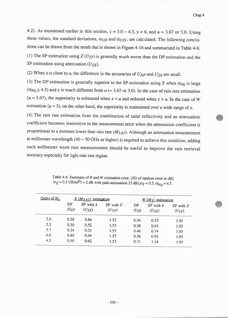
Chap.4
4.2).As mentioned earlier in this section, x - 3.0 - 4.3,! = 6, and, u _ 3.67 or 3.0. Usingthese values, the standard deviations, oryo and oy5V, arra calculated. The following conclu-
sions can be drawn from the result that is shown in Figure 4-16 and summarized in Table 4-6:
(1) The SP estimation using Z (Usi is generally much worse than the DP estimation and theSP estimation using attenuation (USx).
(2) When x is close to a, the difference in the accuracies of Uop and U5; are small.
(3) The DP estimation is generally superior to the SP estimation using X when crlsg is large(or,rO > 4.5) and x is much different from u (= j.67 or 3.0). In the case of rain rate estimation(u - 3.67), the superiority is enhanced when r < u and reduced when x > u.In the case of W
estimation (u = 3), on the other hand, the superiority is maintained over a wide range of x.
(a) The rain rate estimation from the combination of radar reflectivity and an attenuationcoefficient becomes insensitive to the measurement error when the attenuation coefficient isproportional to a moment lower than rain rate (Mz.oil. Although an attenuation measurementat millimeter wavelength (40 - 50 GHz or higher) is required to achieve this condirion, addingsuch millimeter wave rain measurements should be useful to improve the rain retrievalaccuracy especially for light rain rate region.
Table 4-6 Summary of R and IVestimation error. (SD of random error in dB)GX = 0.5 (SD(oq = 2 dB with parh-attenuarion 25 dB),of = 0.5, oN' = 4.5.
DP
(b)
SP withた sP with z
(3哺 (1/sn
SP withた sP with z
(1/sx) (υsy)DPの
3 . 0
3 . 3
3 . 7
4 . 0
4 . 3
0.28
0.30
0。34
0.40
0.50
0.84
0。52
0。33
0.44
0.62
1 . 5 3
1 . 5 3
1 . 5 3
1 . 5 3
1 . 5 3
0.34
0.38
0.46
0.56
0。7 1
0.33
0.45
0.74
0.95
1 . 1 4
1.95
1。95
1.95
1.95
1.95
1 0 4 ‐
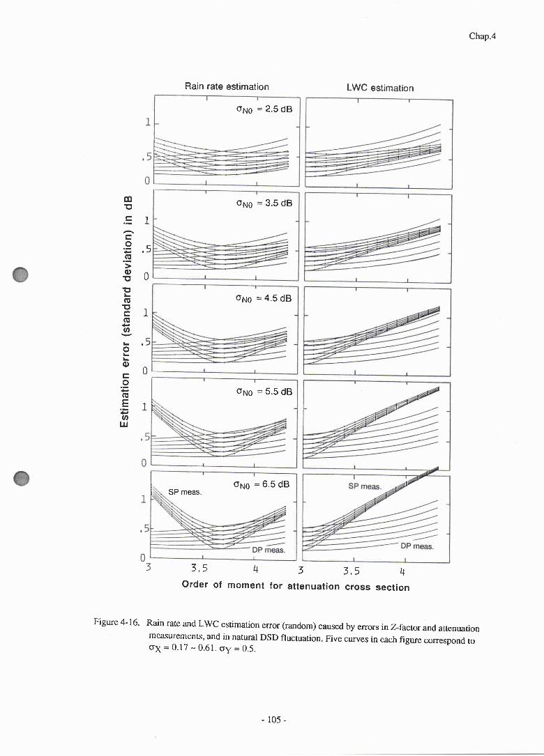
Chap.4
Rain rate estimation
oNo = 2.5 dB
LWC estimation
oNo = 3.5 dB
1
5
0
1
・5
0
・
m「
E¨(Eo〓何一>00
「』0「E”“∽)
」0」』o
EO〓”F』〓∽Ш
3,5 4 3 3 ,5 4order of moment for attenuation cross section
Figure 4-16' Rain rate and LWC estimation error (random) caused by errors in z-factorand attenuationmeasurements, and in natural DSD fluctuation. Five curves in each figure correspond tooX = 0 .17 - 0 .61 . oy = 0 .5 .
oNo = 4.5 dB
σNO=5。 5dB
oNo = 6 '5 dBSP meas.
- 1 0 5 -
Chap.4
4 .6 Con c lus ions
In this chapter, we have investigated statistical properties of the parameters of DSDmodeled by the exponential, the gamma and the lognormal models, and of several importantIRPs such as Z factor and rain rate. The DSD parameters have been derived by means of theMoM (the method of moments) using two or three higher order moments.
It is found that the gamma and exponential DSD parameters are approximatelylognormally distributed except for the shape parameter, m, which has both positive andnegative values. The pdf s of the gamma DSD paramer er mand the lognormal DSD parirmetero2 have long tail at their large values, which is caused by a small fluctuation in the DSD shapeat intermediate to large dtop diameters and it may not be essential to use such large m and. ovalues to estimate other IRps through DSD parameFr estimation.
The parameter A has a clear negative correlation with R and with Z, whlleNg (forgamma models with m fixed to a small value of 0 - 3) and N1's show no or only a smallpositive correlation. This is partly caused by the fact that the higher order moments a_regenerally more sensitive to the variation of A than those of NgorNT. physical DSD evolutionprocesses may also contribute to the higher correlation between A and,Z (orR).
Several important IRP relationships includin g Ze-R,k-R and k-Zerelations have beenobtained through a regression analysis of IRPs derived from the disdrometer data. Theresultant IRP relations (particul arly Ze-R relation) are somewhat different from those obained.assuming the typical exponential DSD models, which is a result of the departure of DSDshape from the exponential form (more concave-down). This suggests that the use of theconventional exponential DSD models are not necessarily the best to assess various IRprelationships- As an alternative, we suggest the use of the "two-parameter,, gamma DSDmodels with n fixed to 3 or 6 shown in Table 4-2 as typical gamma DSD models. From theregression analysis betweenZ andR with a 2-month segmentation, it was found that there issome seasonal dependence of Z-R relation; Z-R relations for winter rainfall are generally lessvariable and give higher Z factors for the sirme rain rate value than those in other seasons.
In order to test the validity of dual-paramerer (Dp) and triple-parameter (Tp)measurements combined with the assumption of the gamma and lognormal DSD models moreprecisely, a simulation of rain rate esdmation has been made. From the simulation, it is shownthat if we can make a TP measurement using two kinds of attenuation in addition to Z, theestimation is nearly perfect, and that even a DP measurement, in which only a kind of
106 -
Chap.4
attenuation can be measured , provides excellent estimation over a fairly wide range of 1, ando values. The rn values of 6-8 and o values of 0.28-0.29 are found to give the lowest RMSelrors in rain rate estimation. Those "best" rn (o) values may shift to small (large) values to
some extent' by considering the possible sensitivity degradation of the disdrorneter. In suchcases' the "best" m would be 4-6. When other lower order moments are estimated from thesilne DP and TP measurements instead of rain rate, the accuracy is degraded and the choice ofDSD model becomes more critical to avoid. large errors. Accord.ing to the result of a zerothmoment estimation, the rn values of around 6 are found to provide the minimum error, whichis similar to the case of rain rate estimation.
Finally, an error analysis has been made to assess the effects of errors in Dpmeasurements. The results indicate that the DP estimation of rain rate and LWC is generallysuperior to the SP estimation under typical measurement error conditions. The superiority ofthe DP estimation is reduced to some extent if the attenuation coefficient is proportional to themoments higher than Ml.ol (rain rate), while the DP estimation becomes insensitive to themeasurement error and the superiority is greatly enhanced if the moment lower than 3.67,i.e., millimeter wave attenuations, can be measured together with Z factor.
107¨
Chap.4
Appendix 4-1 Derivation of DSD parameters
- Gamma parctrneters
From the expression of xth moment of the gammaDSD given by Eq.4.Za,3rd,,4th and6th moments of DSD are written
″3=Ⅳ O「(燿+4)/A″ +4
M4=NO「 (″+5)/A″ +5=NO(溜 +4)F(燿 +4)/A″ +5
(4.Ala)
(4.Alb)
″6=Ⅳ O「 (″+7)/A″ +7=NO(″ +6x溜 +5)(″ +4)F(″ +4)/A″ +7. “ 。Alc)
Eliminating NO「 (″+4)from Eqs.4.Ala and 4.Alb gives
ν4=Oη +4)A-l ν 3・
Sirrlilarly,hm Eqs.4A.lb and 4.Alc,
ν6=(燿 +5)(″+6)A‐2″4・
(4.A2) 玲
(4。A4)
(4.A3)
Eliminating A from Eqs.4.A2 and 4.A3 provides the expression of m in terms of themoments,
(“+4)2/[(″+6)(閉+5)]=″ 43/[ν32ν 6]=G。
Eq'4.A4 yields the solution for m that is given by Eq.4.3. Once we have the value of m, theparameters A and Ng are readily obtained from Eq.4.A2 and then 4.A1a.- Lo g rnrmal p ararne t ers
(4.A5a)
(4.A5b)
(4.A5c)
F r o m E年42b,山 e nat u r d b g a H山ms Of n h , yぬand a h m O m e n t t O f t t e b g n o m」 鋏
DSD,ら,ら,L2,at W五tten
Lχ=ムⅣ+χμ+1/2χ2σ2
1y=LN+yμ +1/2y2。2
Lz=珈 +zμ+1/2z2σ2
where LN = ln N1. Eq.4.A5 constitutes a linear simultaneous equation of L1g, p, and 02,which is easily solved for those DSD parameters. Substituting x = 3, J = 4, and, z = 6, wehave the expressions of N1, p and o2 given by Eq.4.6 through 4.g.
‐108‐
Chap.4
References
(1) Ulbrich, C.W., 1983: Natural variations in the analytical form of raindrop sizedistributions, J . Climate Appl. M eteor., ZZ, l7 64-177 5.
(2) Feingold, G. and Z.Ievin 1986: The lognormal fit toraindrop spectra from frontalconvective clouds in Israel. /. Climate Appl.Meteor.,25, 1346-1363.
(3) Marshall, J.S. and W.M. Palmer, 1948: The distribution of raindrops with size.J . M eteorol., 5, 165- 166.
(4) Mielke, P.W., Jr., 1976: Simple iterative procedures for rwo parameter gammadistribution maximum likelihood estimates. ,I. Appt. Meteor.,15, 181-183.
(5) Wong, R.K.W. and N. Chidambaram, 1985: Gamma size d.istribution andstochastic sampling errors. J. Climate Appl. Meteor.,24,568-579.
(6) Waldvogel, A., 1974: The Ng jump of raind.rop spectra. J. Atmos. Sci., 31,1067 - 1078.
(7) Ajayi, G.O., and R.L. Olsen, 1985: Modeling of a tropicalraindrop size distributionfor microwave and millimeter wave applications. Radio ici.,20, 193-202.
(8) Im, E. and K. Kellogg, 1990: Spaceborne radar for rain and cloud measurements:A conceptual design. Proc. GARssg0, college park, MD, 4zs-429.
(9) Joss, J., J.C. Thams, and A. Waldvogel, 1968: The variation of raindrop sizedistribution at Locarono, Proc. Int. Conf. Ctoud physics,369-373.
(10) Chandrasekar, V. and V.N. Bringi, 1987: Simulation of radar reflecrivity andsurface measurements of rainfatl. /. Atmos. Oceanic. Tech.,4, 464-478.
(l l) Atlas, D., C.W. Ulbrich and R. Meneghini, 1984: The multiparamerer remotemeasurement of rainfall. Radio Sci. 19, 3-ZZ.
(lZ) Ulbrich, C.W., and D. Atlas, 1984: Assessment of the contribution of differentialpolarization to improved rainfall measurements, Radio Scf., 19,49-57.
(13) Bringi, V.N., T.A. Seliga, and W.A. Cooper, 1984: Analysis of aircraft hydro-meteor specffa and differential reflectivity (Zpp) radar measurements during theCooperative Convective Precipitation Experiment, Radio Sci., 19, 157-167.
(14) Goddard, J.W.F. and S. M. Cherry, 1984: Quantitative precipitation measuremenrswith dual linear polarisation radar, Preprin ts, 22nd Conf. Radar Meteorol., Zunch,Amer. Meteor. Soc., 352-357 .
(15) Feingold, G. and Z.Levin 1987: Application of the lognormal raindrop sizedistribution to differential reflectivity radar measurement (Z,Op;.J. Atmos. Ocean. Tech., 4, 377-382.
- 1 0 9 -
Chap.5
CgnpTER 5. SDP MEASUREMENT AND TWO-SCNIE DSD MODEL
5. I Concept
In the discussion in Section 2.3.3, we have assumed that the DP measurement
measures two kinds of integral rain parameters (IRPs) in a radar resolution volume. The DP
measgrement has been tested in terms of rain rate estimation accuracy in Chapter 4. In many
cases, however, such "complete" DP measurements arc difficult to perform. The resolution of
IRP measurements combined with the radar reflectivity measurement are usually coarser than
rhe resolution required for the rainfall profiling. This configuration is different from the
complete DP measurement. As briefly mentioned in Section 2.3.4, we call this type of dual-
parameter measuements "Semi" DP (SDP) measurementl).
l,-et Lr and AR be the resolutions for the first and second measurements, respectively,
and let us assume that Ar is the resolution required for the profiling. In DP measurements, Ar
= AR, and in SDP measurements, AR = n.Lr where n > 2. Similar definitions apply to the
time resolution. Considering that SP measurements need the estimation of one of the two DSD
parameters based on empirical or theoretical models, an SDP measurement with n + "o m&Y
approach an SP measurement. The concept of DP, SDP and SP measurements is illustrated in
Figure 5- 1.
Even from the SDP measurement, through proper DSD modeling, it is possible to
obtain DSD information with the resolutions AR or Ar. Since the first rain parameter is
measured with the resolution Ar, one DSD parameter can be estimated with the same
resolution, while the other DSD parameter can only be estimated with the resolution AR. Thus
the parameters of a DSD modet used for the SDP measurement should have two scale spatial
variabili ty Lr and AlR. We hereafter call this type of DSD model defined over a time or spatial
region (or both) "two-scale" DSD model. Examples of SDP measurements by a spaceborne
radar combininEZfactor profile and a low resolution attenuation data are illustrated in Figure
S-Z(a).It should be noted that ttre DSD parameters used for a two-scale model need not be the
parameters appearing in the original expression of the model for individual DSD. We could
select the DSD parameters in such a way that one of them is most variable and the other is
least variabte, or that one of them is most sensitive and the other is least sensitive to the IRPs
of interest.
l l 0 -

Chap.5
DP
meas。
△RSDP
meas。
SP
meas.
Figure 5-1. Concept of DP, SDP and SP measuremens using radar reflectivity factor (4 ndmicrowave attenuation (&) for rainfall profiling with the resolution Ar.
In a wide sense, the SDP measurement may be recognized as an addition of a broad
rain parameter characterized over a space or time (need not be a radar measurable quantiU) to
the original SP radar measurement with high resolution, and the two-scale model parameters
may be recognized as the conversion of those measured quantities to more fundamental or
useful rain parameters. For example, let us consider the radar-gage comparison illustrated in
Figure 5-2(b). The radar measurement would provide a 4-D map of Z factor with a high
spatial and temporal resolution, while the rain gage would provide a l-D (on the time axis)
profile of the other IRP, rain rate, at a certain spatial location. However, a sequence of gage
samples has to be employed to estimate a time invariant rain paftmeter such asZ-R relation to
avoid errors caused by a spatial discrepancy between the gage and radar measurement
volumes. Thus, the gage data are recognizedas a quantity having a crude temporal resolution,
and we have to assume that the parameter estimated at the gage site is applicable to an entire
raining area and/or storrn life. In summary, the 4-D Z-factor map and the rain gage data at a
point are connected in terms of a two-scale DSD model, in which one of the two DSD
parametsrs is assumed to be constant over the 4-D raining space.
Zl Z2 Z3 Z4
kl k2
←
1 1 1 -
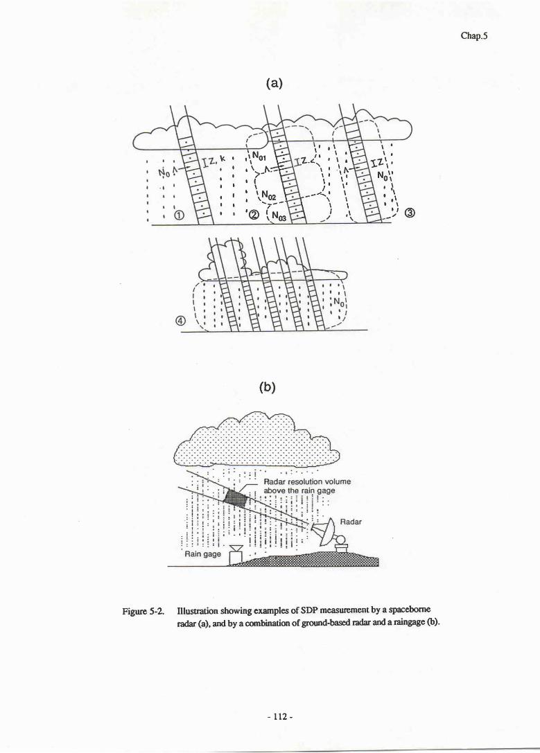
Chap.5
(a)
l 'l o
1z\,Noti
: \: , \
r t
(b)
Figpre 5-2. Illustration showing examples of SDP measuement by a space;borne
radar (a), and by a combination of ground-based radar and a rainpge (b).
③
0
0
0
0
0
0
ヽ
―
ノ
V”へヽヽ、ノ(
■・
rl■
==下‐ヽヽ‐、ヘ
.②(N“
k
o
o
o
o
o
o
- t t z -
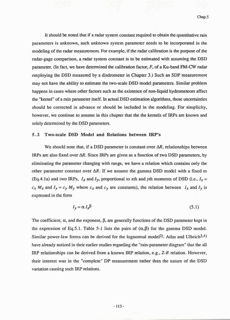
Chap.5
It should be noted that if a radar system constant required to obtain the quantitative rain
parameters is unknown, such unknown system parameter needs to be incorporated in the
modeling of the radar measurement. For example, if the radar calibration is the purpose of the
radar-gage comparison, a radar system constant is to be estimated with assuming the DSD
parameter. (In fact, we have determined the calibration factor, F, of a Ku-band FM-CW radar
employing the DSD measured by a disdrometer in Chapter 3.) Such an SDP measurement
may not have the ability to estimate the two-scale DSD model pammeters. Similar problem
happens in cases where other factors such as the existence of non-liquid hydrometeors affect
the "kernel" of a rain parameter itself. In actual DSD estimation algorithms, those uncertainties
should be corrected in advance or should be included in the modeling. For simplicity,
however, wo continue to assume in this chapter that the the kernels of IRPs are known and
solely determined by the DSD parameters.
5.2 Two-scale DSD Model and Relations between fRP's
We should note that, if a DSD parameter is constant over AR, relationships between
IRPs are also fixed over AR. Since IRPs are given as a function of two DSD parameters, by
eliminating the parameter changing with range, we have a relation which contains only the
other parameter constant over AR. If we assume the gamma DSD model with a fixed m
(Eq.4.la) and two IRPs, Iaand/y, proportional to.rth andyth moments of DSD (i.e., Ix=
cx Mx and /y = cy M, wheta cy and cy are constants), the relation between I, and/, is
expressed in the form
I y=u l r9( 5 . 1 )
The coefficient, G, and the exponent, F, *" generally functions of the DSD parameter kept in
the expression of Eq.5.1. Table 5-1 lists the pairs of (a,F) for the gamma DSD model.
Similar power-law forms can be derived for the lognormal modet2). Atlas and Ulbrich3'4)
have already noticed in their earlier studies regarding the "rain-parameter diagram" that the all
IRP relationships can be derived from a known IRP relation, e.9., Z-R relation. However,
their interest was in the "complete" DP measurement rather than the nature of the DSD
variation causing such IRP relations.
- l t 3 -

Chap.5
Table 5-l Coefficient a and exponent p in tte rain parameterrelationships for the gamma DSD model.
Parameter kept in a
N7
(C/CrP)Not-P G/crFYvrr-P (C/Cr1tx-t
1(m+y+L)/(m+x+l) ylx
Note: Cx= crl(m+x+l), Cy = cy tr(rn+Fl)
Although in most profiling algorithms, power-law IRP relations @q.5.1) are assumed
without detailed discussion on their relation to the p5p5-10), we see that such an assumption
implies the use of a "two-scale" DSD model and that all IRP relations are determined from the
two-scale model parameter assumed to be constant over AR. A preliminary study to determine
a path-averaged DSD parameter from joint measurements of the Ku-band FM-CW radar (see
Chapter 3) and a 12-GHz radiometer has been performed by Kozu et a1.11). Their result
appears to support the validity of the method, although they did not generalizethe nature of
such DSD estimation processes.
Let us consider two-scale models assuming a gamma DSD with m ftxed in which Ng,
N7 or A is constant over AR (see Table 5-1). In these two-scale models, B depends only on
m and the two-scale model assumed, itnd cr depends on the DSD parameter (N0, NTor A) as
well. Thus, estimating the DSD parameter constant over AR is equivalent to estimating a. The
estimation of cr from an SDP measurement was proposed by Meneghini et al.5), Lin et d.6)
and Meneghini and NakamuralO). the concept of the two-scale model gives a physical basis
for such IRP relation adjustment. Instead of adjusting cr, it should be possible to adjust F ot
to adjust both cr and F bV employing other two-sca1e models.
5.3 Proper Two-Scale Model: Empirical Evidence
The question that arises is what is the proper two-scale model. For example, if we
assume that A is constant over AR, then we have linear IRP relations. The same happens if
we assume a very large ln value. These assumptions, however, do not seem to apply to many
cases. Irt us consider Z-Rrelations where x=3.67 andy = 6. If NTis constant, we have the
exponent B of 1.63 (see Table 5-1). Whereas if NO is constantwith mvalues between 0 and
8, we have the exponents between 1.5 and 1.18.
A均
1r4 -
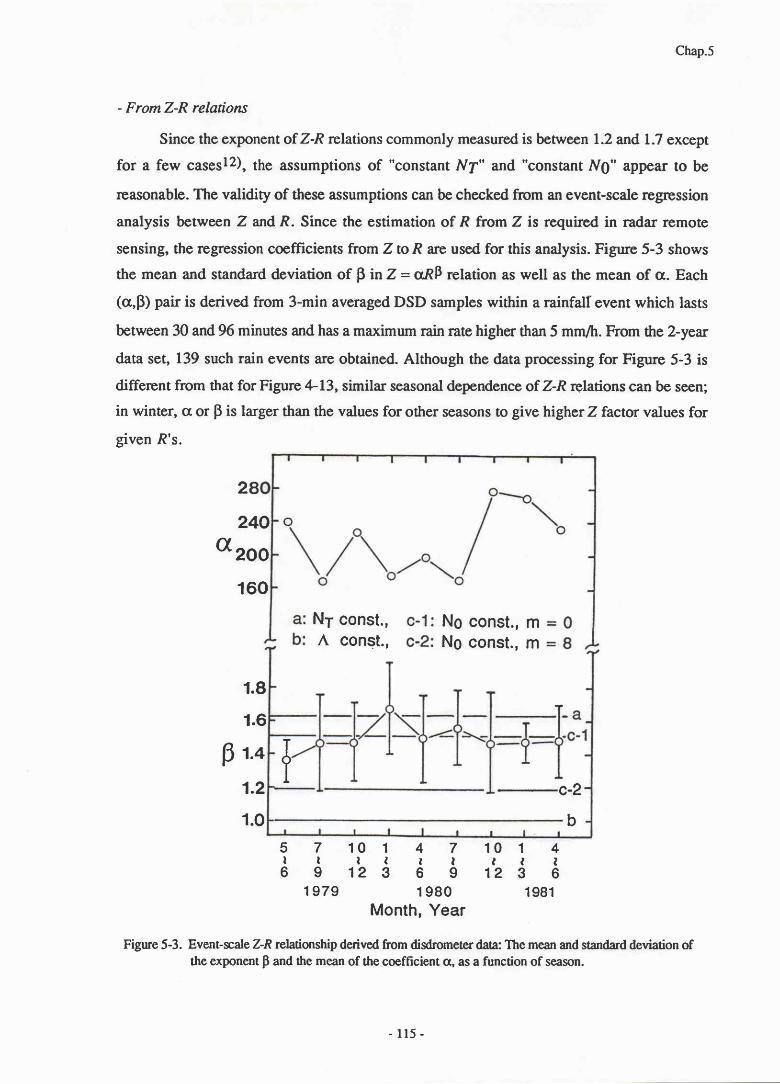
Chap.5
- From Z-R relations
Since the cxponent of Z-R relations commonly measured is between 1.2 and 1.7 except
for a few casesl2), the assumptions of "constant N?n" and "constant N0" appear to be
reasonable. The validity of these assumptions can be checked from an event-scale regression
analysis between Z and R. Since the estimation of R from Z is required in radar remote
sensing, the regression coefficients from Z to R are used for this analysis. Figure 5-3 shows
the mean and standard deviation of p in Z = aRF relation as well as the mean of a. Each
(a,P) pair is derived from 3-min averaged DSD samples within a rainfall event which lasts
between 30 and 96 minutes and has a maximum rain rate higher than 5 mmlh. From the 2-year
data set, 139 such rain events are obtained. Although the data processing for Figure 5-3 is
different from that for Figure +L3, similar seasonal dependence of Z-R rebrtons can be seen;
in winter, cr or p is larger than the values for other seasons to give higher Z factor values for
given R's.
2
240
α200
160
1。8
1。6
β l。4
1。2
1。0
conste,
const。,
const。,m
const。,rn
NT
A
NO
NO
TAY上
4
こ
6
‐89
1
‥
3
‐
0
‥
2
7
1
9
089
4
こ6
1
1
こ
3
0
1
2
97
7
こ
9
9
5
1
6
― c‐2
b
Month, Year
Figure 5-3. Event-scale Z-R relationship derived from disdrometer data: The mean and standard deviation ofthe exponent p and the mean of the coefficient q,, as a function of season.
-115‐
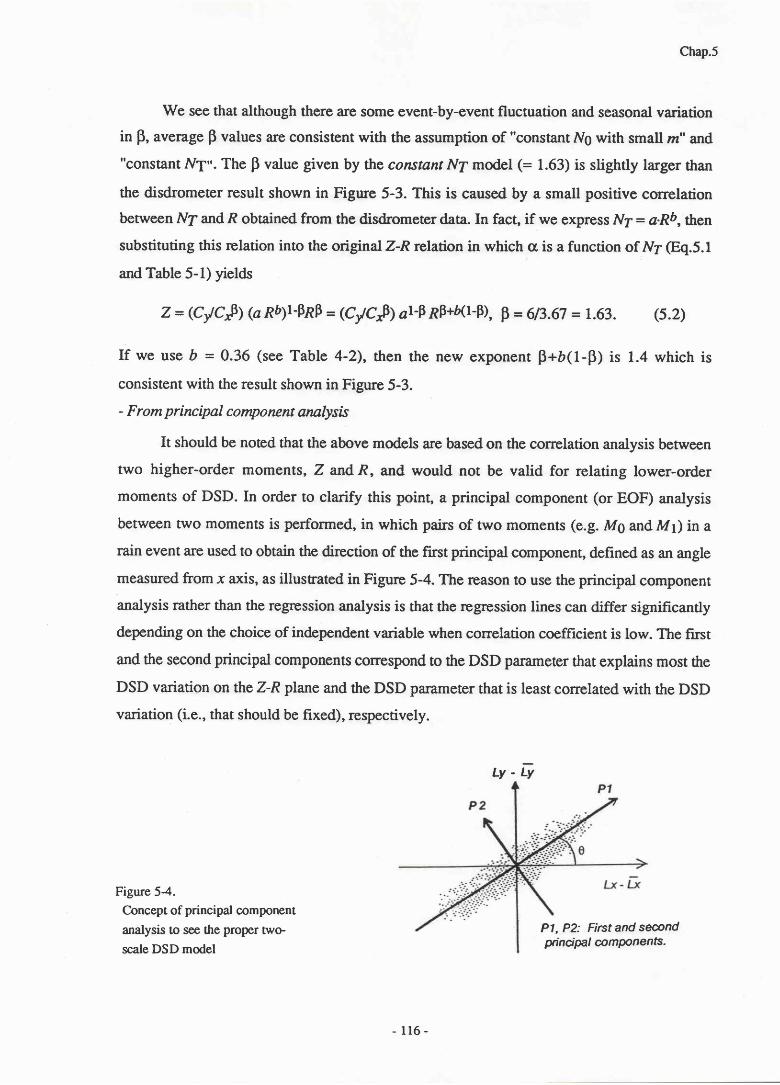
Chap.5
We see that although there are some event-by-event fluctuation and seasonal variation
in F, average p values are consistent with the assumption of "constant Ng with small rn" and,
"constant NT".The p value given by the constant N7 model (= 1.63) is slightly larger than
the disdrometer result shown in Figue 5-3. This is caused by a small positive correlation
between N7 and R obtained from the disdrometer data. In fact, if we express Nr: a-Rb, then
substituting this relation into the original Z-Rrelation in which cr is a function of N1 @q.5.1
and Table 5-1) yields
Z=(C/C♪ )(α Rb)1‐pRβ=(C/C∫ )αl‐β Rβ+ズ1-β),β=6/3.67=1。 63。 (5。 2)
If we use D = 0.36 (see Table 4-2), then the new exponent p+D(l-p) is 1.4 which is
consistent with the result shown in Figure 5-3.
- From principal component annlysis
It should be noted that the above models are based on the correlation analysis between
two higher-order moments, Z and R, and would not be valid for relating lower-order
moments of DSD. In order to clarify this point, a principal component (or EOF) analysis
between two moments is performed, in which pairs of two moments (e.g. MgandM)ina
rain event are used to obtain the direction of the first principal component, defined as an angle
measured from x axis, as illustrated in Figure 5-4. The reason to use the principal component
analysis rather than the regression analysis is that the regression lines can differ significantly
depending on the choice of independent variable when correlation coefFrcient is low. The first
and the second principal components correspond to the DSD parameter that explains most the
DSD variation on the Z-R plane and the DSD parameter that is least correlated with the DSD
variation (i.e., that should be fixed), respectively.
L y -
Figure 5-4.
Concept of principal component
analysis to see the proper nvo-
scale DSD model
一け
Pl, P2: First and seandgincicnl @mrynents.
1 1 6 -
りo VS0
Figrue 5-5. Argument of the fust
principal component of two
moments obtained from event-
scale analysis together with
the arguments assuming typical
twescale models.
Figure 5-5 shows the result of the EOF analysis for various combinations of moments.
Curves in the figure represent the ilguments assuming several two-scale models; "constant No
(m = 0)", "constant Nr " and "constant A". As indicated in the figure, the two-scale model
which is consistent with the result of the principal component analysis depends on the
moments of interest; the "constant A" model is suitable to explain the relation between lower
order moments, while the "constant NO (z - 0)" and "constant NT" models are suitable for
higher order moments just as we have seen in the regression analysis of Z and R.
The above conclusion on the two-scale models suitable for relating higher order
moments may be due to the following facts:
(1) As discussed earlier, higher-order moments are less sensitive to the variation in Ng orNT
and more sensitive to the variation in A than lower-order moments. In other words, A
generally has higher conelation with R and Z thanNg and N7.
Chap.5
N、 const.
鮨 =0
´ゝ
´ ・
a
b
c
d
0
0
7
5
範鮨
M6M4M3M 2
(〇
)
卜ZШZO一〓00 コく」
【OZ
【∝住 卜∽α
【」 」0 卜ZШ〓つOαく
M6M4
117‐
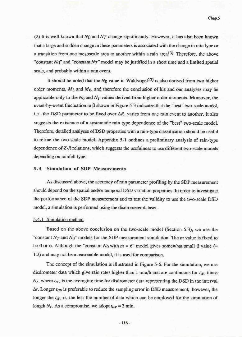
Chap.5
(2) It is well known that Ng and N7 change significantly. However, it has also been known
that a large and sudden change in these parameters is associated with the change in rain tlpe or
a transition from one mesoscale area to another within a rain areal3). Therefore, the above
"constant N0" and "constant Nf" model may be justified in a short time and a limited spatial
scale, and probably within a rain event.
It should be noted that the Ng value in Waldvogell3) is also derived from two higher
order moments, M3 andM6, and therefore the conclusion of his and our analyses may be
applicable only to the Ng and N7 values derived from higher order moments. Moreover, the
event-by-event fluctuation in p shown in Figure 5-3 indicates that the "best" two-scale model,
i.e., the DSD parameter to be fixed over AR, varies from one rain event to another. It also
suggests the existence of a systematic rain type dependence of the "best" two-scale model.
Therefore, detailed analyses of DSD properties wittr a rain-type classification should be useful
to refine the two-scale model. Appendix 5-1 outlines a preliminary analysis of rain-type
dependence of Z-R relations, which suggests the usefulness to use different two-scale models
depending on rainfall tlpe.
5.4 Simulation of SDP Measurements
As discussed above, the accuracy of rain parameter profiling by the SDP measurement
should depend on the spatial anilor temporal DSD variation properties. [n order to investigate
the performance of the SDP measurement and to test the validity to use the two-scale DSD
model, a simulation is performed using the disdrometer dataset.
5.4.1 Simulation method
Based on the above conclusion on the two-scale model (Section 5.3), we use the
"constant Nr and Ng" models for the SDP measurement simulation. The rn value is fixed to
be 0 or 6. Although the "constant No with m = 6" model gives somewhat small p value (=
1.2) and may not be a reasonable model, it is used for comparison.
The concept of the simulation is illustrated in Figure 5-6. For the simulation, we use
disdrometer data which give rain rates higher than 1 mmlh and are continuous for fay times
N7, wheft tav is the averaging time for disdrometer data representing the DSD in the interval
Ar. Longar tsy is preferable to reduce the sampling error in DSD measurement; however, the
longer the tay is, the less the number of data which can be employed for the simulation of
length N7. As a compromise, we adopt tav - 3 min.
- r 18 -

Chap.5
The total time to construct a radar measurement path of N7 =32 is 96 minutes, which
may correspond to an attenuation measurement integrated over a storrn; i.e., estimating IRP
relations on a storm basis. On the other han4 since the 3-min average implies that DSD is
averaged over about I km in range (assuming the drop fall velocity is 6 m/s), smaller N7
values (2 to 4) may represent a single observation by spaceborne or airborne radars in which
path lengths are short.
We assume that the Z (= cz'MO) profile and path-averaged attenuation coefficient [1=
c*-M+) can be measured. Path-integrated attenuation, A, is related to E byE = Al(Nr.Ar).
First, we derive an N6 estimate. Using the k-Z relation shown in Table 5-1, we have
た =
慟%二叫
〓イb1
・J均
等,“〓‐
%上叫
(5。3)
where 6 = (m+5)l(m+7), Cruo = [cp-f(m+5)1.[cr-f(m+l)]-D and <Npl-b> is the path-
averagedN0l-b weighted by Zb.Eq.5.3 states that theNg estimxlg <Ngl-b> is expressed as a
function of -k
and aZ-factor profile, that is
DPmease
averaged disdrorneter data
SDPmeas.
Attenuation resolution
Nr
1
1 1 2 0 o o コ
[- e6 min.-ISPmeas.
2 yeお
Figure 56. Concept of SDP measurement simulation with the disdrometerdata.
32
‐119‐

Chap.5
where CNT =, fc1r'l(m+5)l-[cr'tr(m+7)l'2t3'f@+l)l/3. Using thc IVO ot N1 estimates, A
べ、1‐b>=Chb‐11路π/1当ζ′j = 1
simuad.theノ鴨‐weighted ptth‐avttd Nrlβ,drlJ3p,is JVen by
ミ_lβ>=cN子1鳩π/土 Z3・第
′=1
R, = cRtr(rr+yrl) <UOt-b>U$'b) / tVm+v+r
R; - cR[tr(z+yrl)lF(m+l)] flrrBr3 / Nr
or using the direct integration over D,
Ri = *.tta'+rrt!-b)irfrl D"*3eIil-Ap)dD' 6 v o
R; - Ldru3r'I '@)ffi#" expclr D)dD- o0
(5.4)
(5。5)
(5.6a)
(5。6b)
(5.7a)
(5。7b)
(5。8a)
(5。8b)
Further, a rain rate profile is obtained with the DSD paramcteru; using a moment
apprroximation to rain ratc, i.e. R = cR My where cn b a constant and T =3.67
where Af is glVen by Eq。5。6a or 5。6b,andッcD)iSthe dmp鷲】彙」nal velocity Q.2。H).
‐1 2 0 ‐
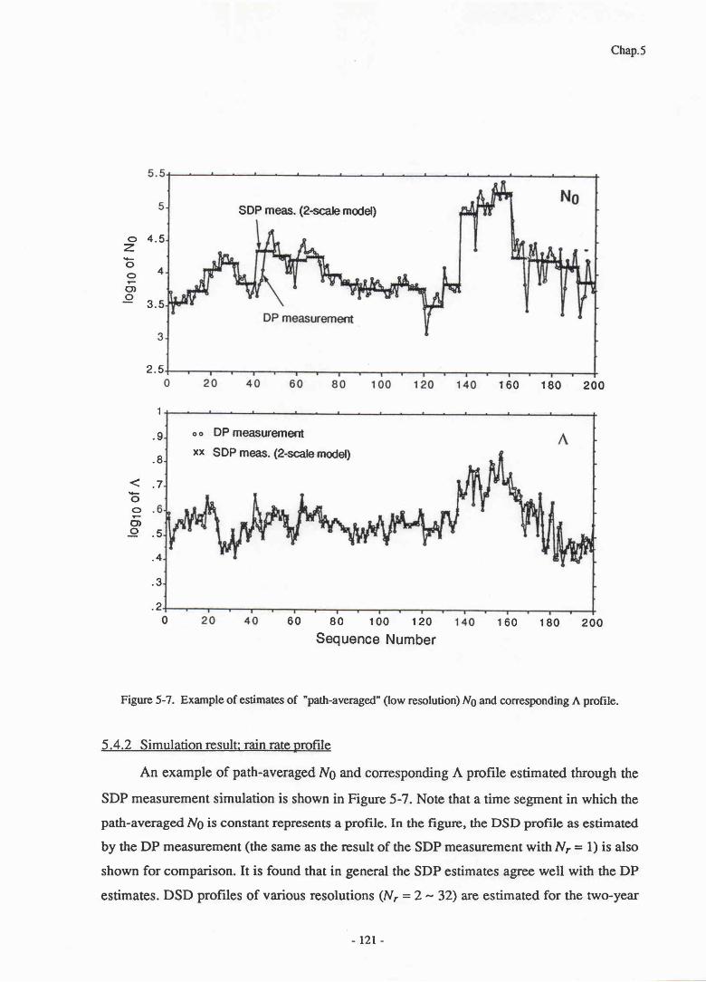
Chap.5
SDP meas. (2-scale model)
5
4
5
4
3
oZ一〇o,02
く
一〇
o一〇2
2 . 5
1
. 9
. 8
. 7
. 5
. 4
. 3
. 2
160 180 200
160 180 2000 6 0 8 0 1 0 0 1 2 0
Sequence Number
Figure 5-7. Example of estimates of 'path-averaged" (low resolution) Ng and coresponding A prof,rle.
5.4.2 Simulation result: rain rate profile
An example of path-averaged Ng and corresponding A profile estimated through the
SDP measurement simulation is shown in Figure 5-7. Note that a time segment in which the
path-averaged Ng is constant represents a profile. In the figure, the DSD profile as estimated
by the DP measurement (the same as the result of the SDP measurement with Nr = 1) is also
shown for comparison. It is found that in general the SDP estimates agree well with the DP
estimates. DSD profiles of various resolutions (N, = 2 - 32) are estimated for the two-year
121
oo DP measurement
xx SDP meas. (2-scale model)
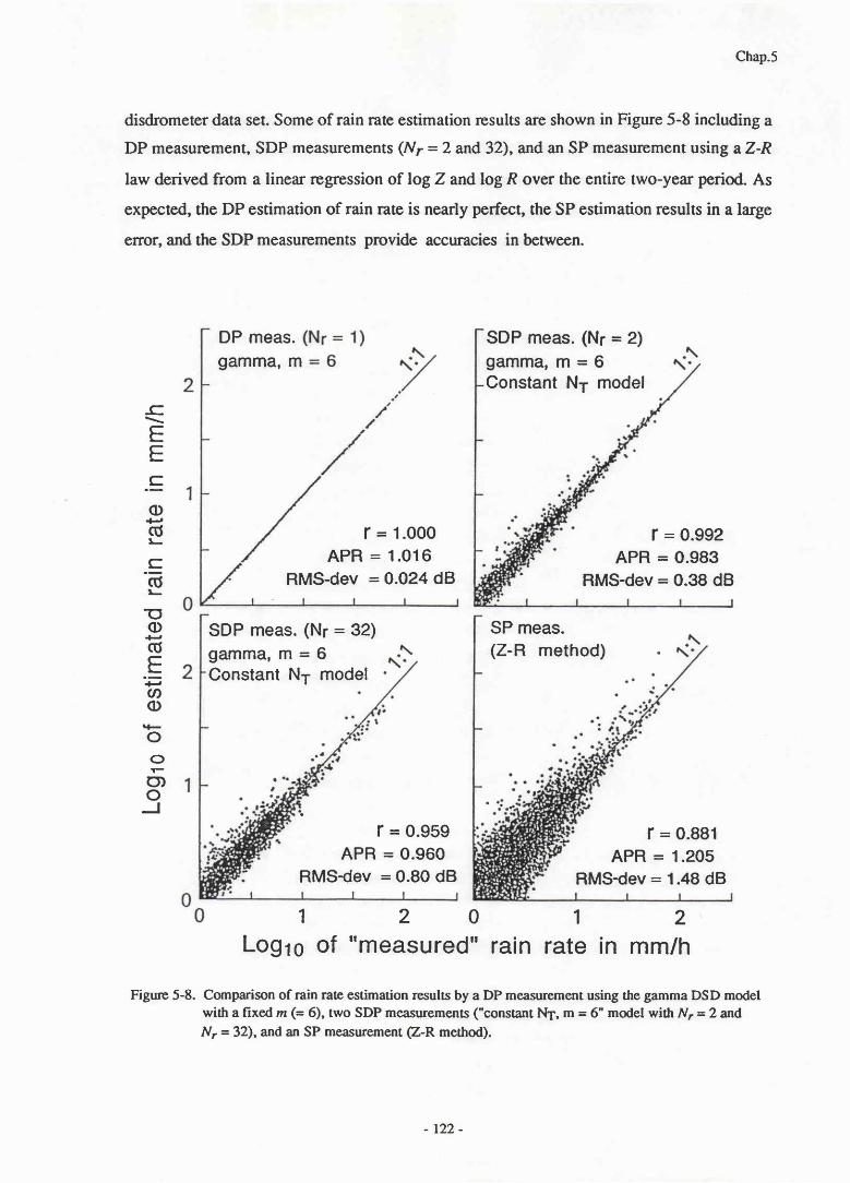
Chap.5
disdrometer data set. Some of rain rate estimation results are shown in Figure 5-8 including a
DP measurement, SDP measurements (Nr = 2 and32), and an SP measurement using aZ-R
law derived from a linear regression of log Z and log R over the entire two-yqr period. As
expected, the DP estimation of rain rate is nearly perfect, the SP estimation results in a large
eror, and the SDP measurements provide accuracies in between.
SDP meas. (Nr = 32)gamma, fTl = 6Constant NT model
r=0.959
APR=0.960
RMS― dev=0.80 dB
12012Logro of "measured" rain rate in mm/h
Figure 5-8. Comparison of rain rate estimation results by a DP measurement using the gamma DSD modelwith a fixed m (= 6), two SDP measurements ("constant N1, m = 6" model with Nr = 2 mdNr = 32), and an SP measurement @-R method).
〓ヽ⊆Lヒ ⊂一 ①一“」
⊂一0」
O①一∞匡上一∽① 一〇
orOOJ
DP meas.gamma, m
r=1.ooo
APR=1。 016
RMS― dev =0。 024 dB
SDP meas. (Nr = 2)gamma, fl'l = 6Constant N1 model
r=0.992
APR=0.983
RMS― dev=0.38 dB
SP mease
(Z‐R method)
r=0。 881
APR=1.205
RMS― dev=1。 48 dB
-122‐
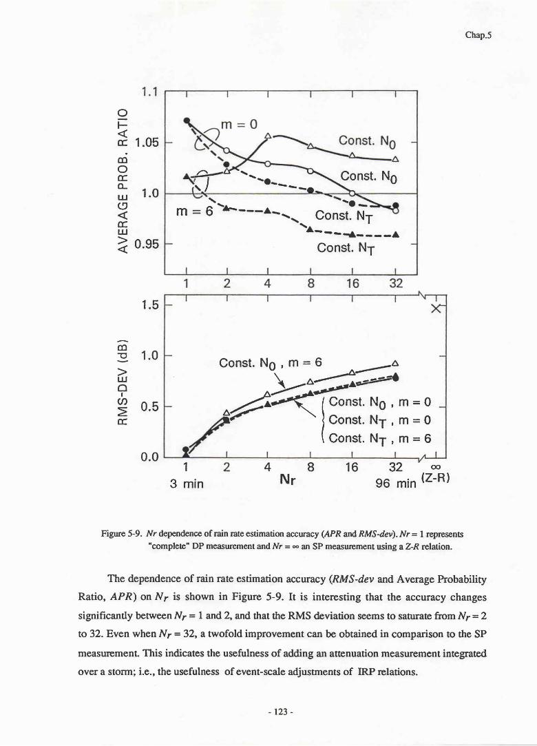
Chap.5
〇一卜<∝
。mO∝」ШO<∝Ш><
1。05
1.0
0。95
⌒m「}>ШOo∽ヽこ∝
1。5
1.0
0。5
Conste Nヽ^<'F"^"t.No, Fn=o
- l Const. N1 , ITI = O
\ Const. NT , fil = 6
0。01
3 min
84 16 32 ‐ ∞
96 min (z-R)Nr
Figure 5-9. Nr dependence of rain rate estimation accuracy (,4PR and RMS-dev). /Vr = 1 represents"complete" DP measurement and Nr = "o an SP measuement using aZ-R relation.
The dependence of rain rate estimation accuracy (RMS-dev and Average Probabiliry
Ratio, APR) on N7 is shown in Figure 5-9. It is interesting that the accuracy changes
significantly between N7 = I and 2, and that ttre RMS deviation seems to saturate from Nr = 2
to 32. Even when N r : 32, a twofold improvement can be obtained in comparison to the SP
measuremenL This indicates the usefulness of adding an attenuation measurement integrated
over a storm; i.e., the usefulness of event-scale adjustments of IRP relations.
(つr′̀~``ヽ・ヽヽ_ ヽ nsto NO
\ A - r r r { r - - - A
Const. N1
123‐
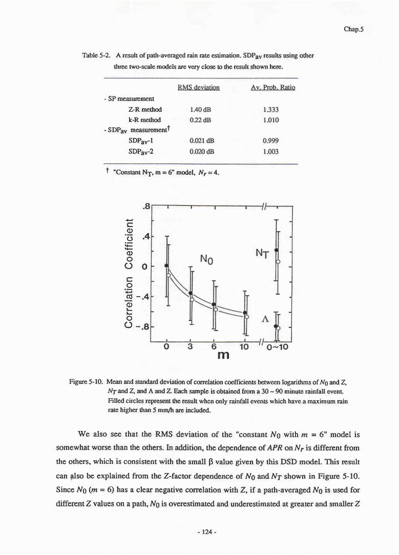
Chap.5
Table 5-2. A result of path-averaged rain rate estimation. SDPav results using other
three two-scale models are very close o the result shown here.
- SP measuement
Z-R method
k-R method- SDPav measurernentt
sDPav-l
sDPav-2
t "Constant N1, m = 6" model, N7 = {.
。4
0
。4
。8
一
一
“C〇一0一〓000 c〇一〕“一①ヒ00
Figure 5-10. Mean and standard deviation of correlation coefficients benveen logarithms of Ng andZ,Nl and Z, and A and Z.Each sample is obtained from a 30 - 90 minute rainfall evenL
Filted circles represent the result when only rainfall events which have a maximum rainrate higher than 5 mm/h are included.
We also see that the RMS deviation of the "constant No with m -- 6" model is
somewhat worse than the others. In addition, the dependence of APR on Np is different from
the others, which is consistent with the small p value given by this DSD model. This rcsult
can Also be explained from the Z-factor dependence of Ng and N1 shown in Figure 5-10.
Since NO (rn = 6) has a clear negative correlation with Z, if a path-averaged Ng is used for
different Z values on a path, Ng is overestimated and underestimated at greater and smaller Z
m
‐1 2 4 ‐

Chap.5
values, respectively. This results in overestimation and underestimation of rain rate at higher
and lower rain rates, respectively. Accordingly , APR, which gives larger weights on higher
rain rates, increases. The result shown in Figure 5-9 indicates that an unreasonable two-scale
model would degrade the rain rate estimation accuracy.
5.4.3 Estimation of path-averaged rain rate
It should be noted that the above results are those for the rain rate estimation for each
resolution cell; i.e. profiling. In estimating a path-averaged rain rate, the SDP measurement
works as a DP measurement since the radar resolution required is now AR, not Ar. There may
be t'wo options for estimating the path-averaged value: (I) Z-tactors are averaged and
combined with the path-averaged attenuation (SDPavl); (2) rain rate profile obtained from the
SDP measurement is then averaged over the path (SDPav2).
A simulation of these "averaged" SDP measurements has been performed and the path-
averaged rain rate estimation accuracy compared with two kinds of SP measurements; Z-P.
method and k-R method. For the SP measurements, Z-R and &-R relations derived from the
two-year disdrometer data are used The result, which is summ arrzed in Table 5-2, shows that
the two SDPav methods glve nearly perfect estimation just as the complete DP measurement.
The k-R method gives slightly larger RMS error than the SDP4y rressurements; however it
still provides an excellent estimation. This is due to the similarity in the kernels of rain rate and
attenuation (assumed to be proportional to M+). The bias error seen in the Z-P. method may be
due to the difference in the data bases for obtaining the Z-R relation and for the simulation.
5.5 Validity of the two-scale model
The validity of the two-scale DSD model can be seen by some different ways. One is to
see the variation of Ng or N1 with range. In SDP measurements, a path-averaged Ng (or N7)
is estimated and used for all range bins. Although this is not uue, our interest is how high the
correlation remains with range. Figure 5-11 shows the scattergram of "true" (the value
estimated by a complete DP measurement) versus path-averaged Ng values for Nr = 2 and Ny
=32 cases. We can see that even when Nr = 32, a high correlation remains. Therefore in
contrast with SP measurements which always assume a fixed Ng or N1 value, SDP
measurements estimating NO or N7 with a low resolution can improve the rain rate estimation
accuracy depending on the measurement resolution and the spatial correlation of the DSD
parameters.
r25 -
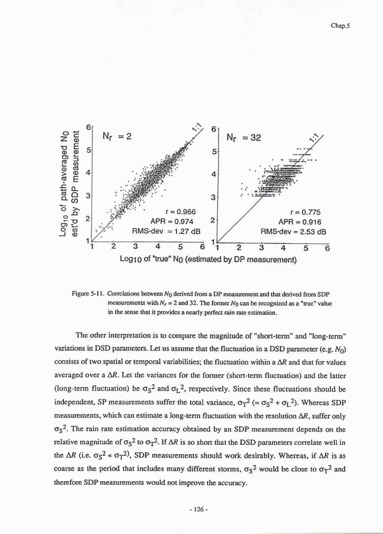
Chap.5
“⊂ΦEδ」⊃∽“Φ“』」∩∽
ゝ0
「い一∽①
OZ
0000」①>C・〓““Q
一〇
〇r00コ
Nv -2 Nr =32
° ° r=o.966
APR=0.974
RMS‐ dev=1.27 dB
r=0。 775
APR=0。 916
RMS‐ dev=2.53 dB
3~4 3 61行~「 ~丁 -7-可
LogtO of "true" Ng (estimated by DP measurement)
Figure 5-ll. Correlations betweenNg derived from a DP measurementand that derived from SDPmeasuremenS with Nr=2and32. The formeril0 can be recognized as a "true" valuein the sense that it provides a nearly perfect rain rate estimation.
The other interpretation is to compare the magnitude of "short-term" and "long-term"
variations in DSD parameters. Let us assume that the flucnradon in a DSD parameter (e.g. Ng)
consists of two spatial or temporal variabilities; the fluctuation within a AR and that for values
averaged over a AR. I-et the variances for the former (short-term fluctuation) and the latter
(long-term fluctuation) be o52 and o12, respectively. Since these fluctuations should be
independent, SP measurements suffer the total variance, of (= oS2 + ot?). Whereas SDP
measurements, which can estimate a long-term fluctuation with the resolution AR, suffer only
oS2. The rain rate estimation accuracy obtained by an SDP measurement depends on the
relative magnitude of o52 to af .If AR is so short that the DSD parameters correlate well in
the AR (i.e. o52 .. oT2), sDP measurements should work desirably. whereas, if AR is as
coarse as the period that includes many different storrns, oS2 would be close to o12 and
therefore SDP measuriements would not improve the accuracy.
‐126‐
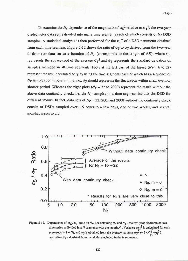
Chap.5
To examine the N7 dependence of the magnitude of o52 relative to o.f , the two-year
disdrometer data set is divided into many time segments each of which consists of N7 DSD
samples. A statistical analysis is then performed for the o52 of a DSD parameter obtained
from each time segment. Figure 5-12 shows the ratio of o5 to 01 derived from the two-year
disdrometer data set as a function of N7 (corresponds to the length of AR), where o5
represents the square-root of the average o52 and oT represents the standard deviation of
samples included in all time segments. Plots at the left part of the figure (Nr = 6 to 32)
represent the result obtained only by using the time segments each of which has a sequence of
N7 s:unples continuous in time; i.e., o5 should represents the fluctuation within a rain event or
shorter period- Whereas the right plots (Nr = 32 to 2000) represent the result without the
above data continuity check; i.e. the N7 samples in a time segment include the DSD for
different storms. In fact, data sets of Nr = 32,200, and 2000 without the continuity check
consist of DSDs sampled over 1.5 hours to a few days, one or two weeks, and several
months, respectively.
1。0
0。8
0。6
0。4
0.2
0。05 0 20 50 500 1000 2000
0一一“匡 卜り
ヽ∽o
100
Nr
200
Figtuc 5-12. Dependence of os/cT rado onlVr.For Obtaining σs and CT,the two‐year disdrometer data
器 TF芦器 :濫 蠍 柵 諾 wTはh
町 iS d i r∝d y c a l c u l a t e d k》m t h e a l l d a t a i n d u d e d i n t h e N s e g m e n t s .
-'.-t ) nverage of the results
=e= I ror Np = 1o -32
With data continuity check
* Results for Nr's are very close
▽ A
▲ NO,
O NO,
m=6
m=o
to this.
127-
Chap.5
The following conclusion can be drawn from Figure 5-12: (1) os /or approaches
unity, i.e. SDP measurements approach SP measurements with increasing Nri (2) there
appears a gap between the results obtained from the data sets with and without the continuity
check, indicating the existence of large event-by-event DSD variations; (3) NO (m = 6) and A
have larger os/o1 ratios than No (m = 0) and Nr; and (4) SDP measurements should
improve the rain rate estimation accuracy by about a factor of two, with some dependence on
the assumed two-scale model. The latter two conclusions, which indicate the necessity to use
a "good" two-scale model and the validity of applying a two-scale model within a rain event,
are consistent with the result shown in Figure 5-9. In the case of Ng (m = 0), for example, o1
is as large as 5 dB (see Table 4-l); however, 05 within a rain event is only about 2 - 2.5 dB.
The gap in the o5/o1 ratio mentioned in (2) suggests that the rain rate estimation accuracy
would be degraded if the resolution AR (in this test, a time segment of length Ny') spans over
two or more different rain events.
5 .6 Conc lus ions
In this Chapter, we have investigated rain rate estimation properties of the "semi" dual-
parameter (SDP) radar measurement combining radar reflectivity factor (Z) and a path-
integrated microwave attenuation through a simulation using a disdrometer data set collected
over 2 years. This type of measurement applies to most of spaceborne radar measurements,
and has properties between " complete" DP and single-parameter (SP) measurements. We
have proposed a concept of "two-scale" DSD model, the parameters of which can be derived
from the SDP measurement.
It has been shown that the SDP measurement provides an RMS error ranging from 0.4
to 0.8 dB for the estimation of log of rain rate in contrast with 0.03 dB and 1.5 dB for a DP
measurement and an SP measurement (Z-R method), respectively. The degradation in the
accuracy from DP to SDP measurements comes mainly from the decorrelation in DSD
parameters. An interesting result is ttrat even when the resolution of attenuation measurement
is as coarse as N7 = 32 (96 minutes), the SDP measurement clearly provides a better
estimation than the SP measuremenl This indicates the usefulness of "event-scale" adjustment
of IRP relations. It is shown that the SDP measurement can also improve the accuracy in
comparison to SP measurements (k-R and Z-R methods) in the estimation of path-averaged
rain rate.
128‐

Chap.5
The ability of the SI)P measurementto estimate】 DSE)parameters should generally be
desirable fbr introducing a clear physical background into rain pararneter estimation algonthins
and for dceper understanding of precipitation propertieso For rain rate cstimation, the
usefulness of the SDP measurement should be enhanced as the kemel of attenuation differs
from that of rain rate.If the differcnce is small,like 35‐GHz attenuation,the SDP
measurement would not be so useful;i.e.DSE)estimation may not be necessary.Moreover,
the usefulness should“ pend on the relative rnagnitude of dle・・long―te■lll・
・DSE》 variation and
measurement erors as we have studied in Chapter 4 for the dual― pattllneter rneasurement.If
the fo.1ller is very large,even somewhat poor lneasurernents should be useful.If I〕 SI)is
stable,the SDP FneaSurelllent may be more cIToneous than dle SP IIleasurement.
I n t h e p r e s e n t s t uむ,wc h a V e a s s u m e d t h a t I R P s a r e pЮpom o n a l t o D S D m o m e n t s t o
s i m p l i f y t h e f o m u l a t i o n . A l t h o u g h t h i s i s a p pЮxim a t e l y m e f o r m a n y c a s e s , i n g e n e r a l w e
h a v e t o u s e m o r e s o p h i s d c a t e d o r n u m e r i c a l t e c h n i q u e s t o d e五ve D S D p a r a m e t e r s ; p a r t l c u l a r l y
when effects oflMie scatteHng and rain attcnuadon up to a radar scatte五 ng v。lume become
signiflcant. Through such generalization, however, va五 ous rain rate profiling methods
combining a Z―factor proflle and a padl attenuation could be recastin tems of the pararncter
estimation of a two―scale DSI)model. An approach that is applicable to more general
conditions w11l be proposed later in Chapter 7 as well as a test of the FnethOd using an alrcraft
dataset.
Although the two scale rnodels used in the present study should be adequate ones as a
flrst approximation,the acctracy in estimating rain rate and other rain parameters should be
improved by reflnements of the two―scale model◆Such reflnements include DSD modeling
incorporating a rainfall―type dependencc ofthe two― scale model and a height dependence of
DSE)caused by evaporation,coalescencc,breakup,ctc.,and modeling the lDSE)of b五 ght―
band particles especially for the application to spaceborne radar measurements. As an
extension of the SDP measurement,combining two(or more)kindS Of path… integrated
quantities will a Z―factor profile is also wortt studying for obtaining a better estimation of the
DSE)pararneters.
‐129-
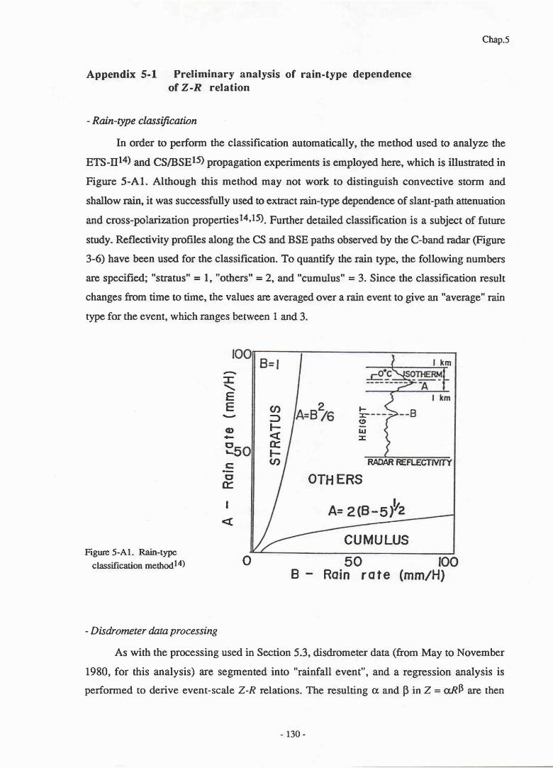
Chap.5
Appendix 5-1 Preliminary analysis of rain-type dependenceof Z-R relation
- Rain-type classification
In order to perform the classification automatically, the method used to analyze the
ETS-trla) and CS/BSEIS) propagation experiments is employed here, which is illustrated in
Figure 5-A1. Although this method may not work to distinguish convective storm and
shallow rain, it was successfully used to extract rain-type dependence of slant-path attenuation
and cross-polarization propertiesl4'15). Further detailed classification is a subject of future
study. Reflectivity profiles along the CS and BSE paths observed by the C-band radar (Figure
3-6) have been used for the classification. To quantify the rain qpe, the following numbers
are specified; "stratus" = l, "others" -2, and "cumulus" = 3. Since the classification result
changes from time to time, the values are averaged over a rain event to give an "average" rain
type for the event, which ranges between 1 and 3.
=ヽ
EE
O
路C
●
∝
:
く
Figure 5-Al.Rain‐ type
classiflcation inedlod14) 0 50 :00B― Rcin ra↑e(mm/H)
- Disdrometer dnta processing
As with the processing used in Section 5.3, disdrometer data (from May to November
1980, for this analysis) are segmented into "rainfall event", and a regression analysis is
performed to derive event-sc ale Z-R relations. The resulting c and p in Z: crRF are then
∽⊃卜くに卜∽
OTH ERS
A= 2(B- Slz
卜〓0一ロエ
RADAR IttFECTIVrY
CUMULUS
130-
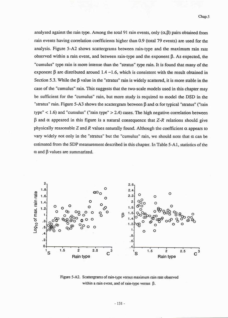
Chap.5
analyzed against the rain type. Among the total 91 rain events, only (a,F) pairs obtained from
rain events having correlation coefficients higher than 0.9 (total 79 events) are used for the
analysis. Figure 5-A2 shows scattergrams between rain-type and the maximum rain rate
observed within a rain event, and between rain-type and the exponent p. As expected, the
"cumulus" t54)e rain is more intense than the "stratus" type rain. It is found that many of the
exponent p are distributed around 1.4 -I.6, which is consistent with the result obtained in
Section 5.3. While the p value in the "stratus" rain is widely scattercd, it is more stable in the
case of the "cumulus" rain. This suggests that the two-scale models used in this chapter may
be sufficient for the "cumulus" rain, but more study is required to model the DSD in the
"stratus" rain. Figure 5-A3 shows the scattergram between F attd c for typical "stratus" ("rain
type" < 1.6) and "cumulus" ("rain t54)e" >2.4) cases. The high negative correlation between
p and a appeared in this figure is a natural consequence that Z-R relations should give
physically reasonable Z andR values naturally found. Although the coefficient o appears ro
vary widely not only in the "stratus" but the "cumulus" rain, we should note that cr can be
estimated from the SDP measurement described in this chapter. In Table 5-A1, statistics of the
cr and p values are summarized.
0“0」C一“』.X“C』一〇
0,00コ
2
1 . 8
1 . 6
1 。
1.2
1
.6
.4
.2
0
2.
2.4
2.2
20
0
θ
0 00
0
0 ° 0 1 .
1 .
ト1.4
1 .
1.5 2 2.5
Rain type
喀°0♂ °Ъ°o0 0
、 ■5日Jfv"25 c 3C
Figure 5-M. Scattergrams of rain-t1pe versus maximum rain rate observed
within a rain event, and of rain-type versus p.
-131-
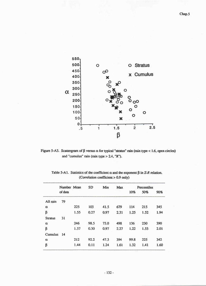
Chap.5
α
1。5
β
2。5
Figure 5-A3. Scutergram of p versus cr for typicat'strants'rain (rain t)?e < 1.6, open circles)
and 'cumulus" rain (rain type > 2.4,"X").
Table 5‐Al.Statistics ofthe coefrlcicllt αand the exponent β in z_R rehtion.(COrelatiOn coefrlcierlt>o。9 only)
550
500
4
4 0
3 5
3 0
2 5
200
15
1
O
X
Stratus
Cumulus
00。 0
00
0 °
Number Mean SDofdaa
Min 血 Percendles
10% 50% 9070
All rain
α
β
Smtus
α
βCumulus
α
β
79
31
225
1。55
246
1.57
2 1 2
1 . 4 4
103
0.27
98.5
0。30
92.2
0 . 1 1
41.5
0.97
73.0
0.97
47.3
1.24
679 114
2.31 1.25
498 136
2.27 1。22
394 99。 8
1。61 1.32
215 345
1.52 1.94
230 390
1.53 2.01
225 342
1.41 1。 60
0
14
132‐
Chap.5
References
(1) Kozu, T. and K. Nakamura, 1991: Rainfall parameter estimation from dual radar
measurements combining reflectivity profile and path-integrated attenuation.
J. Atmos. Ocean. Tech.,8, 259-270.(2) Feingold G. and Z.l-ein, 1986: The lognormal fit to raindrop spectra from frontal
convective clouds in Israel. J. Climate Appl. Meteor.,zl, 1346-1363.(3) Atlas, D. and C.W. Ulbrich, 1974: The physical basis for attenuation-rainfall
relationships and the measurement of rainfall parameters by combined attenuation and
radar methods . J . Res. Atmos., 8, 27 5-298.(4) Ulbrich, C.W., and D. Atlas, 1978: The rain parirmeter diagram: Methods and
applications. J. Geophys. Res., 83, (C3), 1319-1325.(5) Meneghini, R., J. Eckerman, andD. Atlas, 1983: Determination of rainrate from a
spaceborne radar using measurements of total attenuation, IEEE Trans. Geosci.Remote Sens., GE-21, 34-43.
(6) Lin, H., M. Xin, and C. Wei, 1985: Ground-based remote sensing of LWC in cloudand rainfall by a combined dual-wavelength radar-radiometer system.Advances in Atrnas. .Sci., 2,93-103.
(7) Weinman, J. A., C. D. Kummerow, and C. S. Atwater, 1988: An algorithm toderive precipitation profiles from a downward viewing radar and multi-frequencypassive radiometer. Proc. GARSS88, Edinburgh, U.K., 229-234.
(8) Fujita, M., 1989: An approach for rain rate profiling with a rain-attenuating frequencyradar under a constraint on path-integrated rain rate, Proc. GARSS 89, Vancouver,Canada, L49L-L494.
(9) Marzoug, M. and P. Amayenc, 1991: Improved range profiling algorithm of rainfallrate from a spaceborne radar with path-integrated attenuation constraint.IEEE Trans.Geosci. Remote Sens., GE-29, 584-592.
(10) Meneghini, R. and K. Nakamura, 1990: Range profiling of the rain rate by anairborne weather radar. Remote Sens. Environ, 31, 193-209.
(11) Kozu, T., J. Awaka, K. Nakamura, and H. Inomata, 1986: Improved estimation ofrain attenuation and rainfall rate for slant-paths by simultaneous radar and radiometermeasurements. Preprints,23rd Conf. Radar Meteor., Snowmass, CO, Amer.Meteor. Soc., 104-107.
(I2) Battan, L.J., 1973: Radar observation of the atmosphere.The University ofChicago Press, Chicago, 324pp.
(13) Waldvogel, A., 1974: The N6 ju-p of raindrop spectra. J. Atmos. Sci.,31,1067 -1078.
(14) Furuham&, Y., T. Ihara, T. Shinozuka, K. Nakamura, and J. Awaka, 1981:Propagation characteristics of millimeter and centimeter waves of ETS-[ classifiedby rainfall types. Ann. Telecomm., 36, 24-32.
(15) Fukuchi, H., T. Kozu, K. Nakiunura, J. Awako, H. Inomata, and Y. Otsu, 1983:Centimeter wave propagation experiments using the beacon signals of CS and BSE
- 1 3 3 -
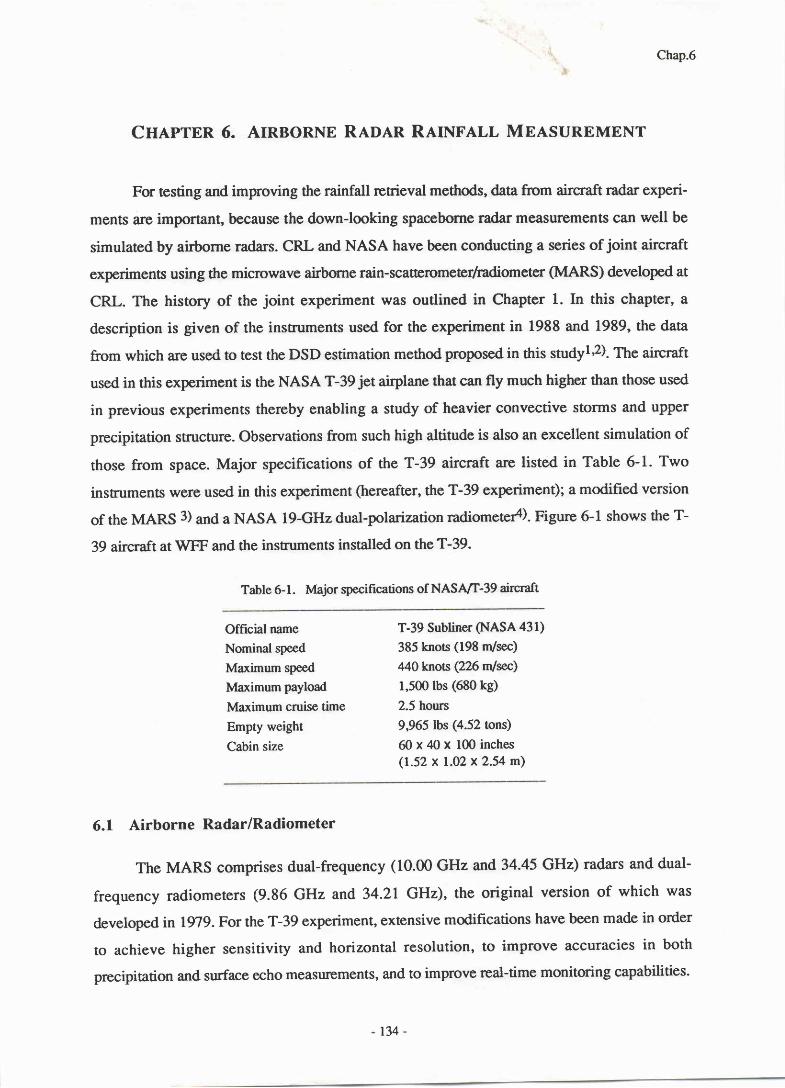
Chap.6
CHIpTER 6. AIRBORNE RnNnR RaTNTALL MEASUREMENT
For testing and improving the rainfall retrieval methods, data from aircraft radar experi-
ments are important, because the down-looking spaceborne radar measurements can well be
simulated by airborne radars. CRL and NASA have been conducting a series of joint aircraft
experiments using the microwave airborne rain-scatterometer/radiometer (MARS) developed at
CRL. The history of the joint experiment was outlined in Chapter 1. In this chapter, a
description is given of the instnrments used for the experiment in 1988 and 1989, the data
from which are used to test the DSD estimation method proposed in this studyl'2)' the aircraft
used in this experiment is the NASA T-39 jet airplane that can fly much higher than those used
in previous experiments thereby enabling a study of heavier convective storrns and upper
precipitation stnrcture. Observations from such high altitude is also an excellent simulation of
those from space. Major specifications of the T-39 aircraft are listed in Table 6-1. Two
instruments were used in ttris experiment (hereafter, the T-39 experiment); a modifred version
of the MARS 3) and a NASA l9-GHzdual-polarization radiometera). Figure 6-1 shows the T-
39 aircraft at WFF and the instruments installed on the T-39.
Table 6-1. lvlajor specifications of NASA/[-39 aircraft
Official name
Nominal speed
Maximum speed
lvlaximum payload
Maximum cruise time
Empty weight
Cabin size
T-39 Subliner sXSA 431)
385 knots(198nげ 餌 )
440 knots(226 Wsec)
1,500 1bs C680 kD
2.5 hollrs
9,965 1bs“.52 ton⇒
60X40x 100 inches
(1.52 x l.02x2.5411L)
6.L Airborne Radar/Radiometer
The MARS comprises dual-frequency (10.00 GHz and34.45 GHz) radars and dual-
frequency radiometers (9.86 GHz and 34.21 GHz), the original version of which was
developed in 1979.For the T-39 experiment, extensive modifications have been made in order
to achieve higher sensitivity and horizontal resolution, to improve accuracies in both
precipitation and surface echo measurements, and to improve real-time monitoring capabilities-
134
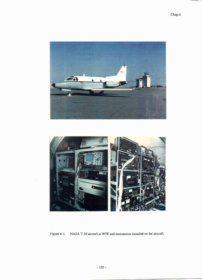
熙打
鸞
Chap.6
Figure 6-1.NASA T‐ 39 aircraFt at―and ins― ens irlstalled on the aircrafL
‐135‐

Chap.6
Major parameters of the instnrments for the T-39 experiment are summarized in Table G2.1\e
blockdiagram of the system is shown in Figure 6-2.\\e system consists of antennas, X-band
and Ka-band radars (RF and IF units), an VKa-band radiometer, a 19-GHz radiometer
(NASA's), a signal processorlradar controller (original one), a CAMAC 5) digitavanalog VO
system, a digital tape drive, a pirctr/roll gyro, a loran receiver, a video cirmera and recorder, an
oscilloscopo, and three IBM PC's (for radar data collection, for 19-GHz radiometer data
collection, and for real-time monitoring, respectively). The major items of the system upgrade
for the T-39 experiment are:
. Antenna: Original offset parabolic antennas were changed to a pair of matched beam horn-
lens antennas having 5-degree half-power beam width (HPBW) and 30-dB gain. Those
provide about 4-dB better sensitivity than and about 40 percent reduction in foot print size
from the values of the original antennas.
. Data processing system: An IBM PC-based new data processing system was developed. To
support various analog and digital VO's, CAMAC instruments and an internal VO board are
used to make interfaces to other equipments.
. Real-time monitoring: Another IBM-PC was installed to provide versatile real-time monitor
functions including two types of color displays; a radarftadiometer system status summary and
color-coded2-D display of the measured radar reflectivity profiles. Data for this real-time
monitor are transmitted from the data acquisition computers through RS-232 interfaces.
. Radar/radiometer data are stored on a 1600-BPI magnetic tape. The summary data sent to the
monitor computer are also stored on a floppy disk to allow a quick review of a flight.
. A CAMAC high-speed 8-bit AID converter provides a radar signal sampling rate of 0.2 psec
that is 2.5 times oversampling in comparison to the radar pulse width. The integrator
connected directly to the A/D converter allows a variable number of pulse integration, Niwrg,
from 1 to 65536, although N;n rcg of 128 is nominally used. The oversampling is useful to
improve the accuracy in measuring surface return signal level because the surface return is
usually very spiky for near-nadir incidence.
. Data sampling window was expanded from the original one (9 l<rn) to 22.5 km (X band) and
20.25 km (Ka band) in order to measure entire storrn including mirror image.
- 1 3 6 -
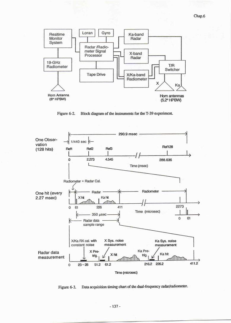
Chap.6
Horn Antenna
(6・HPB崎
R t t R t t R e C
o 2273 4.545
Hom antennas
(12°HPBⅥo
288.636
Figure 6-2. Block diagram of the instmments for the T-39 experimenl
290.9 msec
One(Dbser‐
vation
(128 hn→
One hit (every2.27 msec)
Radar datameasurement
面ise 紳降」
X Syso noise
measurementKa Sys.n《来、o
measurernent
X hn
郎 ~8 51.2 612 aa2 Z発 2
Tmetm―
Figurc G3. Data acquisition timing ctrart of the dual-frequency radar/radiometer.
Ref128
-137-
4112

Chap.6
. Extended noise monitoring function: Two types of noise level monitoring were added; one is
to measure the receiver noise plus a noise from an internal terminator that is used to monitor
short-term (a few minutes to one fiight) receiver gain fluctuation (Noise-ca[), and the otheris
to measure the receiver noise plus the antenna noise which varies depending on microwave
emission properties of the surface (Noise-sys). This is used to extract the signal level from the
measured total (signal + noise) level.
The data acquisition timing chan is shown in Figure G3. The data sampling starts from
5L.2 psec before the X-bandpulse hit in order to measure the noise levels and a leak signal
directly coming from the transmitter. The latter is used to monitor the radar transmit timing.
Table6-2 lvlajor system pammeters for the T-39 experiment
RADAR
Center frequencyAntenna
TypeAperureGainHPBW
TransmitterPeak powerPRFPulse width
ReceiverNoise frgureDetectionDynamic mnge
Signal ProcessorSample intervalRange windowNumber of indep.samples (nominal)
X b a n d
10.00G比
Hom lens
42 cm
30.3 dB
5.2 deg
20 kW
4401・Iz
O.5 rec
5。3 dB
Logarithmic
8 0 d B
O . 2 r e c
22.5 km
128
K a b a n d
34.45 GL
Hom lells
13 cm
304 dB
5。l deg
10 kW
440L
O.5 rec
9.6 dB
Logarimic
80 dB
O . 2陣
20。25 km
128
RADIOMEπ R
Center frequencyAntennaIF bandwidthInteg. timeResolution
Same as the radar antenna1 0 0 M I ・ I z
O.25 sec
O.5K
1001ヴロ[Lz
O.25 sec
O.5K
K b a n d
18。70 GHz
Hom lens
2 0 0 M I‐I z
O . l s e c
O.3K
-138‐
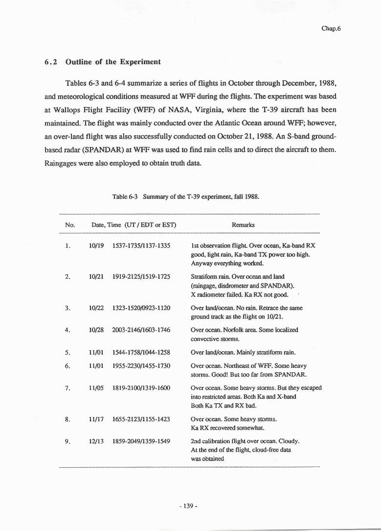
Chap.6
6.2 Outl ine of the Experiment
Tables 6-3 and 6-4 summarize a series of flights in October through December, 1988,
and meteorological conditions measured at WFF during the flights. The experiment was based
at Wallops Flight Facility (WFF) of NASA, Virginia, where the T-39 aircraft has been
maintained. The flight was mainly conducted over the Atlantic Ocean around WFF; however,
an over-land flight was also successfully conducted on October 2t,1988. An S-band ground-
based radar (SPANDAR) at WFF was used to find rain cells and to direct the aircraft to them.
Raingages were also employed to obtain truth data.
Table 6-3 Summary of the T-39 experiment, fdl 1988.
No. Date, Time (UT / EDT or EST) Remarks
1. l0ll9 1537-173511137-1335 lst observation flighr Over ocean, Ka-band RX
good, light rain, Ka-band fi power too high.
Anyway everything wotked-
2. 10t21 1919-212511519-1725 Smadform rain. Overocean and land
(raingage, disdrometer and SPANDAR).
X radiometer failed. Ka RX not good.
3. 10122 1323-152010923-1120 Over land/ocean. No rain. Rerace the sameground track as the flight on lol2l.
4. l0l28 2Cf.3-214611ffi3-1746 Over oceirn. Norfiolk area. Some localized
convective storms.
5. 1llOt 15/.4-175811044-1258 Over land/ocean.ldainly stratiform rain.
6. 1ll01 1955-223011455-1730 Over ocean. Northeast of WFF. Some heavy
storms. Good! But too far from SPANDAR.
7 . LU05 1819-2100/1319-1600 Over ocean. Some heavy storms. But they escaped
ino restricted areas. Both Ka and X-band
Both Ka TX and RX bad.
8. llllT 1655-21231L155-L423 Over ocean. Some heavy storms.
Ka RX recovered somewhaL
9. 12/13 1859-2M9/1359-lY9 2nd calibration flight over ocean. Cloudy.
At the end of the flight, cloud-free data
was obtained
- r 39 -
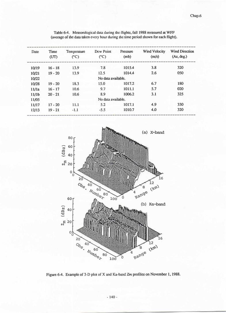
Chap.6
Table G4. Meteorological data during the flights, fall 1988 measured at WFF(average of the data taken evcry hour during the time period shown for each flight).
Time Tempcrature
CttD (°C)
Dcw Polnt Pcsstlre
(°C) (mb)
Wind Vel∝ ity
(nn/S)
Wind l)irection
cAz,“g。)
10/19
10/21
10/22
10/28
11/1a
llノlb
H/05
11/17
12/13
16-18 13.9
19‐ 20 13.9
19-20 18.3
16‐ 17 10.6
20‐ 21 10.6
17‐ 20 11.1
19-21 ‐ 1.1
7.8 1015.4
12.5 1014.4
No data available.
8
6
3
2
0
0
0
0
5
0
0
2
5
8
2
2
3
2
3
0
1
0
3
3
3
15.0
9。7
8。9
1017.2
1011.1
1006.2
6。7
5 . 7
3 . 1
No data available。
5。2 1017.1
-5.5 1010.7
9
0
4
4
( a ) X― b a n d
Ka―band
2
6。
4。
2。
。
(NmO)
日N
0
0
0
6
4
2
(NmO)
EN
%
ご《 ゝ
0ぉ ■ 。。
Fignre 64. Example of 3-D plot of X and Ka-band 7-tnprofiles on November l, 1988.
‐140-
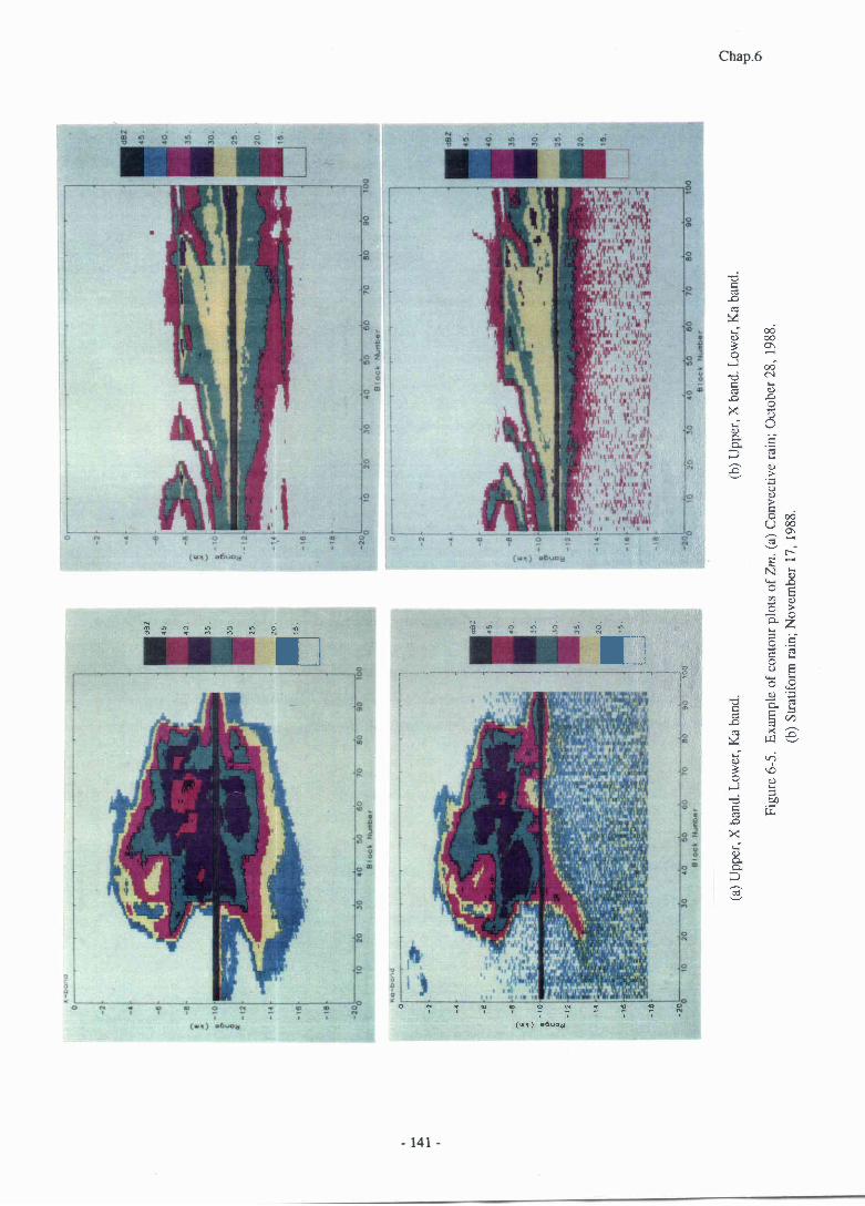
dB
Z
45
.
40
55
10
.
?0
15
.
(a) U
pp
cr, X
ba
nd
. Lo
wcr
, Ka
ba
nd
.(b
) Up
pcr
, X b
an
d. L
ow
er,
Ka
ba
nd
.
Fig
ure
6-5
. E
xiu
np
lc of c
on
tou
r plo
ts o
f Zm
. (a
) Co
nv
ec
liv
c ra
in; O
cto
bc
r 28
, 19
88
.
(b) S
tra
tifo
rm ra
in; N
ov
cm
be
r 17
, 19
88
.
目 墨
「 ― ― ― 1 1 1 1 ‐ ‐ ― ― ― 「 l t l ‐ 1 ・ ― 癬 埒
0
・2
・4
・6 ■ ‐0
‐2
‐4
‐6
‐3 m
( ● 一 ) ● O C Q “
‐ 】 ヽ 】 ‐
0 コ ” つ い

Chap.6
Figure 6-4 shows an example of 3-D plot of X-band and Ka-band Zm profiles
measuredon October 1, 1988, over the Atlantic Ocean. A single observation, which was taken
approximately every 0.4 seconds, represents an average of 128 pulse hits. Since the aircraft
nominal speed is about 200 m/sec, 100 observations correspond to about 8 km if the
observation is continuous. For data processing, however, those observations which were
intemrpted by radio interference, taken during aircraft attitude fluctuation and banking, and
taken over some of non-raining areas have been skipped in order to guarantee the quality of
processed data and to reduce the data volume. The abscissa "observation number" represents
the sequential number after the data skip, and therefore the actual distance is generally larger
than the value simply measured by the above conversion factor (80 meters per observation.)
The sharp large spike at about ll-km below the aircraft shown in Figure 6-4 is the
surface return. Although the quantity Zm for the surface return is meaningless, it is shown to
see its relative magnitude. In most cases, the X-band surface return is almost constant
indicating little rain attenuation at X-band. In the corresponding Ka-band plot, much stronger
rain attenuation is evident from the large variation in the surface return. Below the surface,
mirror image return appears for X-band. For Ka-band, on the other hand, no mirror image
appears due to the strong rain attenuation at this frequency. This feature can be more clearly
seen from the contour plots of Zm valaes. Figure 6-5 shows an example of such plots for
typical convective cell and stratiform rains over the Atlantic Ocean. In the Ka-band plot of the
convective storrn, some mirror image appears at the leading edge of the storrn at which no rain
exists between the precipitation aloft and the surface.
6.3 Radar Equation and Processing of Level "zero" Data
The first step of the radar data processing is the conversion of a "count" value stored on
the tape to the apparent effective radarreflectivity factor,Zm (see Eq.2.23). To do this, radar
equation appropriate to the radar observation condition should be established, and the radar
system constants appearing in the equation should be quantified as well as their temporal drifts
during a time period of interest. Since the radar equation relates the Zm value to the radar
received power, it is necessary to establish another relation; i.e. the relation between the
received power and the count value.
-142-
Chap.6
- Radar eqwfiion used to obtain Zrn valuc
From Eq.(2.23), the radar equation, written in decibel unit, relevant to the observation
condition for the T-39 experiment can be written
P(r)=C+10・ log10 Z″-20・log10 r
widl
C=10・ log10(π3/(10241n2))+2・G+20・ log10 0b+10・log10←π)+Pr
+10・log10 1」【w12_201og10 λ―L-180.0
(6。1)
(6。2)
where Zm (mm6lm\ is the apparent radar reflectivity factor, r (m) is the range from the radar
to a target, G (dB) is the antenna gain, 06 (rad) is the half-power beamwidth of the antenna, c
(m/sec) is the speed of light, t (sec) is the pulse width, P1 (dBm) is the radar peak transmit
power, K,u is the dielectric factor of water 94.2.10), l, (m) is the radar wavelen gth, L (dB) is
the total system loss, and C is the radar system constant. Note that "-180.0" is necessary to
convert the unit of Zmfrom -667p3 to m3.
- Radar received power calibration
The relation between radar received power and count value stored on the tape can be
determined by injecting RF signals of known levels into an input port of the receiver and by
measuring the corresponding count values. Such receiver calibration has been performed by
using a microwave frequency synthesizer as a source. Since the receiver has a logarithmic
detector, the relation between the input signal level, P, and the count value, Y, is expressed as
y=α P ttb (6.3)
where a and b are coefficients to be determined through the linear regression of the measured
values of P and I'. It should be noted that a and b are usually determined through the
calibration using a continuous wave of a single frequency rather than an incoherent signal like
rain echo, and that Y represents the video voltage after the incoherent integration of log-
converted power. Therefore, an end-to-end radar equation to obtain Zm is given by
10.log1g Zm = a Y + b + F6r - C + 20.log1g r (6.4)
where Fbs ?2.5 dB) is the bias caused by integrating the logarithm of powerrather than the
power itself (Section 2.2.3).In practice, there is a small fluctuation in a,b and C. According
143
Chap.6
to our experience, however, the coefficient a is almost constant for a given logarithmic
detector. The fluctuation in C is mainly caused by that in the transmit power, and can be
monitored by measurin E P t periodically. Whereas, the fluctuation in b is caused by the gain
drift in the receiver (including the log detector). Assuming that the noise figure of the receiver
is almost constant at least within a flight (several hours), we can use the noise level oulput
from the receiver as a tool to monitor receiver gain drift when a constant noise power is
injected to the receiver (e.9., the noise from a terminator with temperature controlled). The
Noise-cal measurement mentioned above is made for this purpose. Such monitoring of relative
variation in the transfer function from Y to Zm allows an accurate measurement of "relative"
Zm values.
6 .4 External Radar Calibration
The absolute Zm measurement is morc difficult than the relative measurement because
the bias errors in a, b and C as well as the "relative" fluctuation of those values have to be
taken into account. In practice, however, the bias error in a is minor and the error in D can
effectivety be combined with that in C. Thus, the problem reduces to the determination of the
system constant C. Since the antenna characteristics have to be known to determine C, it is
necessary to employ an external calibration scheme using a reference target. Although there are
several candidates for the reference target such as metal spheres and corner reflectors6), it may
be said that the rain itself is the best target in the sense that the same radar equation as that used
for actual rain observation can be used to determine the error in C.
The radar is externally calibrated by using the data obtained during the over-raingage
flight on Octobr 2I, 1988 (see Figure 6-6). As the rain was widespread and sratified, DSD is
assumed to follow the Marshall-Palmer (MP) distributionT) from which a 10-GHz Ze
(calculated with Mie theory) vs. rain rate relation of 203-R1.6 is derived. A correction factor,
F, in the radar equation, expressed as l0'logtO Zeffue = 10'logt0Zemeas * F, is estimated
from the comparison of Ze*tor and Ztgogt assuming Zegase =Z€ffrr, where Ze*ro,
represents the average of Ze'sjust above the surface (altitudes 300-600 m) and where Zegage:
203 Rgagrl.6,Rgog, being the gage-measuredrain rate. Among the raingages shown in Figure
G6, nine aircraft passages over raingages ilf4 - #10 are used for the calibration. Time tnends of
the raingage-measured rain rates and timing of aircraft passages are shown in Figure 6-7.The
rain rates observed by the gages range from 3 to 18 mm/h. In order to reduce the statistical
- t 4 4 -
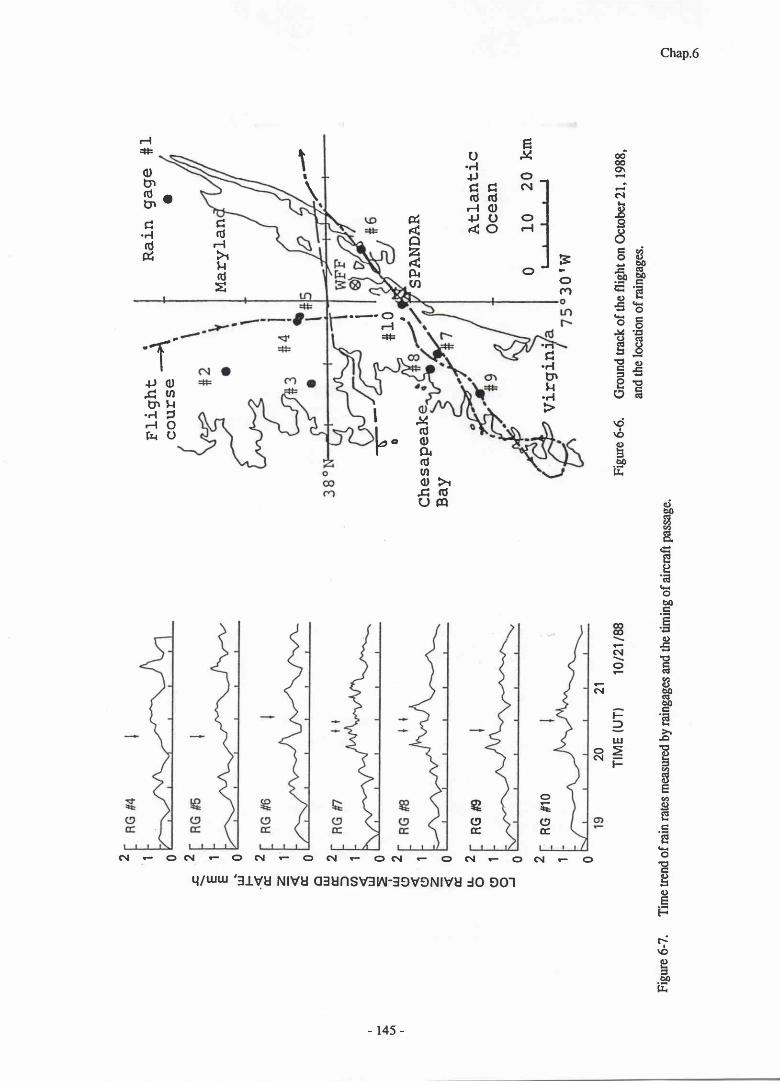
2 1 0 2 1 0 2 1 0 2 1 0 2 1 0 2 1 0 2 1 0
〓 ヽ E E 、 Ш 卜 く ∝ Z 一 く ∝ 口 Ш ∝ ⊃ ∽ く Ш Σ ‐ Ш O く 0 2 一 く ∝ 」 0 0 0 J
‐ 】 ヽ い ‐
::l星::一→ ヘ
|#10
Ra■
n gage
●
Ma
ryla
n
ン・″
SP
AN
DA
R
Atl
an
tic
Oc
ea
n
#l
ヽ~~
0
Ch
es
aP
ea
kB
ay
20 21
TIME IUT) 10/21/88
virg
inj
o ■
0 20 km
1 3 1 o ロ
309W
Fig
ure
6-6
. G
rou
nd
tra
ck of t
he
flig
hto
n O
cto
be
r2l, 1
98
8,
and t
he lo
catio
n of r
aing
ages
.
の コ ” 「 。い
RG JЮ
RG″
10
Fig
ure 6
-7.
Tim
e tre
nd of
rain
rate
s mea
sure
d by ra
inga
ges an
d the
timin
g of a
ircr
aft p
assa
ge.

Chap.6
rain rate variability, temporal averaging (-2 minutes) and spatial averaging(-2 km, along the
flight direction) have been applied to raingage and radar data, respectively. The final F value is
obtained by the average of F values obtained from the 9 passes, using a weighting factor
approximately proportional to the inverse of the sum of three factors; variances of the radar and
gage-derived Ze's and a factor proportional to the distance between raingage site and the
ground foot print of the radar. This methd is applied only to the X-band radar and yields an F
value of I.32 (1.2 dB). The calibrated radarconstant gives the RMS decibel deviation of 1.6
dB for the 9 pairs of Rgage and radar estimated rain rate. Figure 6-8 shows the correlation
between rain rates as measured by the raingages and those estimated from the radar with the
calibrated system constanL
To calibrate the Ka-band radar, we use Ze values far above the bright-band during light
stratiform rains, where it is reasonable to assume that the scatterers are small ice particles
which should satisfy an excellent Rayleigh scattering approximation and cause little attenuation
even at Ka-band. Comparing Ka-band Ze's with the calibrated X-band ones provides an F
value of 0.65 (-1.9 dB) for the Ka-band data. When the same Ka-band radar calibration
scheme is applied to rainfalls observed in other flights, however, approximately tl dB
variation has been found in the Ka-band F value, which is probably caused by an unstableness
of Ka-band receiver that we have encountered throughout the experiment. For the Ka-band
data processing, therefore, the F value is tuned once for each flight.
Figure 68. Conelation benveen
rain rates measured by raingages
and those estimated by the catib-
rated X-band radar using a MP
7z-R relation.
Oct. 2L, 1988
r=0。 73
ジ
0
%
oooo(o
05 r0152025Raingag+neasr-rred Rai:r Rate Grrn^)
5
0
5
0
2
2
■
■
5
0
(く
目
)
3
配
石
配
冒
ヨ
路
巴
石
旧
配
- 1 4 6 -
Chap.6
6。5 Conclusions
The CRL microwave airborne rain scatterometer/radiometer (MARS) was upgraded to
make high altitude aircraft rainfall measurements using the NASA T-39 aircrafr Alttrough the
Ka-band radar transmitter and receiver have sometimes had troubles, the system has worked
well during the fall 1988 experiment. The system upgrade has provided wider range window,
higher sensitivity, and probably higher accuracy in the Zm and surface d measurements than
the original MARS. An external radar calibration has been successfully performed by
employing the rain rate data measured by a raingage network. The calibration of the Ka-band
radar, which is generally difficult due to the large rain attenuation, has been made through a
new scheme; the comparison of Ka-bandhn values with the X-band ones far above the bright
band. This scheme appears to work reasonably well, which leads to the quantitative analysis of
Zrn values that will be described in the next chapter.
The T-39 experiment provided quantitative multiparameter radar and radiometer data
sets from high altitude which is an excellent simulation tool for the measurement from space.
The data would therefore be valuable to test various rainfall retrieval algorithms from space.
We will test the DSD estimation method proposed in Chapter 5 using the T-39 experimental
data.
-147‐
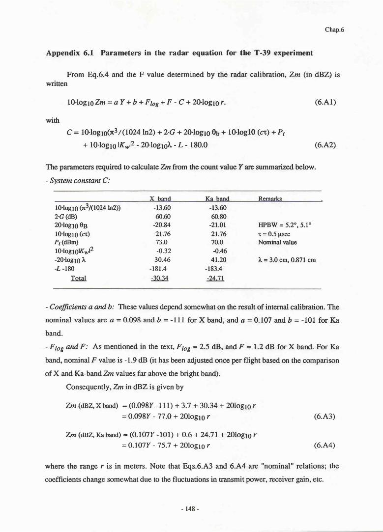
Chap.6
Appendix 6.1 Parameters in the radar equation for the T-39 experiment
From 8q.6.4 and the F value determined by the radar calibration, Zm (in dBZ) iswritten
l0. loglsZm= aY +b + F6t+ F - C +20-logr0r. (6. ,4 '1)
with
C = l0.lolrc(n3 / (lD24ln2) + 2.G + 20.log1s 0u + 10.1og10 (n) + P1
+ 10.1og 16lKr,l2 - 20.log1oL - L - 180.0 (6.A2)
The parameters required to calculate Zrn from the count value f are summarized below.
- System constant C:
X band Ka band Remarks
lO.losro Qc3/(tozqh2) -13.60 -13.602・C cdB)20・log10 0B
10・log10(“ )PrCBm)
10。log10Kッ 12
-20。log10 λ
―Ij-180
Total
60。60 60.80
‐20.84 -21.01 HPBW=5.2° ,5。1°
21.76 21。 76 τ =0.5 μs∝
73.0 70。 O Nominal valuc
-0。32 ‐ 0.46
30.46 41.20 λ =3.Ocm,0.871 cm
‐181.4 _183.4'
-30.34 ‐ 24.71
―Cοψ εJ`“rs α tt bi lhese values depend somewhat on the result ofintemal cahbradon。 ■ e
nonlinal valucs are α =0。098 and b=-11l for X band,and α =0.107 and b=-101 for Ka
band.
―FゎgαたごFf As IIlentioned in the text,Fゎg=2.5 dB,and F=1。 2 dB for X band.For Ka
b a n d , n o m i n a l F v a l u c i s - 1 . 9 d B ( i t h a s b e e n〔可 uSt e d o n c e p e r f l i g h t b a s e d o n t h e c o m p a n s o n
ofX and Ka― band Ztt values far above the bright banの 。
Consequently,Zttin dBZ is given by
Z鷲 (dBZ,X band)=(0。 098y_111)+3.7+30.34+201og10 r
=0。098y_77.0+201og10 r (6.A3)
Zレ電(dBZ,Ka band)=(0.107y_101)+0.6+24.71+201og10 r=0.107y_75。 7+201og10 r (6。 A4)
where the range r is in meters.Note that Eqs.6.A3and 6。 A4are"nominal"relations;the
coefflcients change somewhat due to the nuctuations in mnslnit power,receiver gain,ctc.
-148-

Chap.6
References
(1) Kozu, T., R. Meneghini, W. C. Boncyk, K. Nakamura, and T. T. Wilheit, 1989:Airborne radar and radiometer experiment for quantitative remote measurements
of rain. Proc. /GARSS 89, Vancouver, Canada, L499-I502.(2) Kozu, T., K. Nakamura, R. Meneghini, and W.C. Boncyk, I99l: Dual-paftLmeter
radar rainfall measurement from space: A test result from an aircraft experiment.IEEE Trans. Geosci. and Remote Seru., GE-29, 690-703.
(3) Okamoto, K., S. Yoshikado, H. Masuko, T. Ojima, N. Fugono, 1982: Airbornemicrowave rain scatterometer / radtometer. I nt. J. Remote Sens., 3, 277 -294.
(4) Spencer, R.W., T. T. Wilheit, R. Hood, ild A. Chang, 1987: Prrecipitationdetection with the ER-2 microwave precipitation radiometers. Proc. 2rd AirborneScience Worl<shop, Miami, FL, 93-95.
(5) Cleart, R. T., 1986: The IEEE-583 Bus -- CAMAC, A versatile interface standard.BUSCON, The Users' Conference, San Jose, CA, I-LZ.
(6) Ulaby, F.T., R.K. Moore, and A.K. Fung, L982: Mirowave remote sensing: Activeand Passive. Vol.II. Artech House, Norwood, MA, 457-10@pp.
(7) Marshall, J.S. and W.M. Palmer, 1948: The distribution of raindrops with size.J. Meteorol.,s, 165-166.
- r 49 -

Chap.7
CTTNTTER 7. BXPERIMENTAL TESTS OF SEMI DUAL-PANAMETER
MBnSUREMENT
As shown in previous chapters, statistical analyses of DSD parameters and a simulation
of SDP measurements using the disdrometer data set have revealed that the semi dual-
parameter (SDP) measurement combining a Zm profrle and a path-integrated attenuation can
provide a reasonable improvement in rain rate estimation accuracy through the estimation of
two.scale DSD model parameters. If such SDP measurements could be performed from space,
various useful rainfall properties including Ze-R relations for each observation could be
obtained in addition to the improved rain rate estimates. In practice, however, there has been
no successful experimental result of such DSD estimation until now.
In this chapter, we test the SDP measurement using the data obtained from a joint
aircraft experiment described in Chapter 6 in order to evaluate the perforrnance and limitations,
and further to improve the method. For this test, the SDP measurement is constructed by the
combination of an X-band (10 GHz) radar reflectivity profile and either X- or Ka-band (34.5
GHz) parh anenuarion obtained from sea-surface echo (i.e., by the SRT method). One of the
major problems in such testing is that it is usually very difficult to obtain a good "reference"
measurement. Although the raingage (or disdrometer) data may serve as such reference,
spatial and temporal variability in rainfall can cause a significant error in the comparison of
such point measurements and airborne radar data. The same applies to the comparison of the
ground-based and airborne radars because of the different radar resolution volumes. In the
latter case, the calibration accuracy of the ground-based radar is also a problem. Therefore, we
will employ another approach; consistency between independent measurements. Specifically,
we will use the Ka-band Zrn ptofrle for this consistency check l-3).
7.L Methods of the Test and the DSD Model
7. 1. 1 General discussion
In the simulation described in Chapter 5, we have assumed that the radar reflectivity Ze
and path-integrated attenuation are proportional to 6th and 4th moments of DSD and that Ze is
measured without attenuation in order to simplify the discussion and to obtain an analytical
solution to the equation for the DSD parameters. These assumptions approximately hold for
light to moderate rain rate cases in which the X-band attenuation is negligible and Ka-band
- r 50 -

Chap.7
path attenuation can be measured from the surface return. To handle heavy rain cases,
however, wo need more generalized approach, which will be discussed in this section.
As for the two-scale DSD model necessary for the DSD estimation, we rcfer the results
obtained in Chapter 5, and use the exponential "two-scale" DSD model in which A is variable
with range whereas Ng is constant over the path for each observation. By combining X-band
Zm profile and X or Ka-band path-integrated attenuation, the two-scale DSD model
parameters ar€ derived. In general, a numerical technique is required to derive the DSD
parameters; however, with the assumption of power-law IRP relations (see 8q.5.1), a
simplification is possible, and in some special conditions, the DSD parirmeters can be derived
analytically as described in Chapter 5. An outline of these procedures is shown below.
We begin with the radar equation using "apparent" Ze's at X and Ka band, Zmy,!
being a subscript representing the value at X or Ka band (1l : X or Ka):
ryQ) = Cy lKylz zmr(r) / ,? (7.1)
where Cy is a radar constant,lKylz is a dielectric factor of water, rg is the range from radar to
the fth resolution volume, and Py(r) is a radar received power. Since Zm is a quantity that can
be obtained without any assumption of DSD, apart from bias or random errors in P(r) or C, a
Zmprofile (i.e. nZm's, n being the number of range bins) is recognized as a "measurable"
quantity by a radar. The "tnte" Ze's,Zey(ri), may be relatedtoZmby
ZZy(r3・p=zgyCr3・)exp[-0.21n10 Ay(り] (7.2)
with
ι
Ay(り=Σ εJら(りνノ=1
where ky(rl is the rain attenuation coefficient in dB/unit distance, Ar is the interval between
radar range bins, and e4 = l when j <i and0.5 when j =i.(tu =0.5 means thatAy(r;)
represents ttre attenuation up to the "center" of the range bin t.)
The other quantity we employ here for the DSD estimation is a path-integrated attenua-
tion derived from surface echo (ASR,y) that can be estimated from a difference between
surface return powers (in dB unit) within and outside the rain. ASR,y is expressed as
AsR,y=Σり07)Δr.ノ=1
(7.3)
151
(7。4)

Chap.7
Noting thatZer(1) ana kyf) are functions of DSD parameters at ri,i.e. A(r, andNg, we see
that Zmr(1) is a function of A(rr) through A(t-) and Ng, and A5p,y is a function of A(rr)
through A(rn) and Ng. Thus, generic equations relating measurable quantities and DSD
parameters are
Zttrl)=fxl(Al;fり
ZZx(rり=fx2(Al,A2:NO)
ZHx(ra)=fX″ (Al,A2,… 0,Aが 均 )
勧 施(rl)=fKalい 1;均 )
Zttκα(化♪=fKa2体1,A2;ハb)
Zttκα(%)=fK“ (Al,A2,… 0,A″;NO)
AsRメ =gx(Al,A2,… 0,A″;ⅣO)
AsR,κα=gKa(Al,A2,…0,A″;ⅣO)
(7。5a)
(7。5b)
(7.5c)
(7.5d)
The functions fxi, fr.r, gX, and gra arc the same as Eqs.7.2 and7.4 in nature, but they are
expressed in terms of DSD parameters. In other words, Eq.l.5 is based on the assumption
that the backscattering and extinction cross sections of the hydrometeors are known so that
Zey and ky are expressed solely as functions of the DSD parameters. Although the back-
scattering and extinction cross sections of raindrops depend on temperature to some extent and
there is a small atmospheric gaseous attenuation, the above assumption approximately holds
for the frequencies we consider here. I-ater in this chapter we discuss the attenuation caused
by non-liquid hydrometeors. At present, we continue to assume that the precipitation particles
along the path are all raindrops.
The concepts of the estimation of DSD parameters and other rain parameters are shown
in Figure 7 -I. lf we employ either the X-band or the Ka-band Zm profile @q.7.5a or 7.5b)
and either A5p,y or Agp,yo (8q.7.5c or 7.5d), it is theoretically possible to obtain the n+l
DSD parameters along the path (A(rr) through A(rn) and an No) by inversion techniques from
the n+l measurable quantities. It could atso be possible to employ all X and Ka-band
-152‐
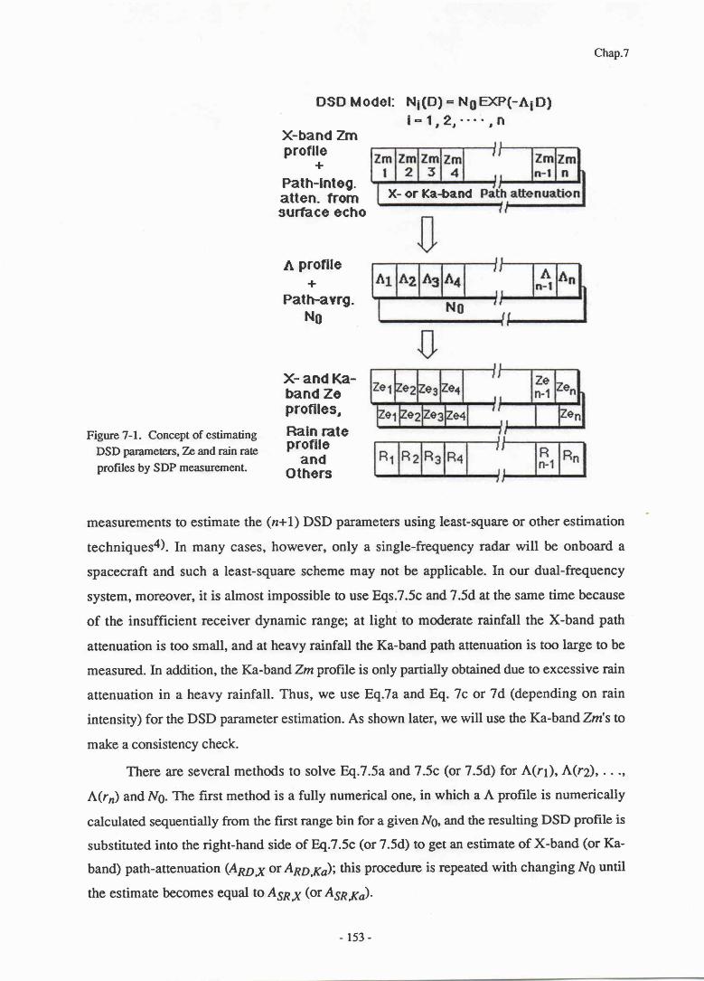
Chap.7
DSD Model: Ni(D) - N0 EXP(-A; D)i : 1 r 2 r " " r f t
Figure 7-1. Concept of estimating
DSD parameters,T* and rain rate
profiles by SDP measurement.
X-band Zmproflle
+Path-lnteg.atten. fromsurface echo
A proflle+
Path-avrg.Ng
X- and Ka-band Zeproflles,
Ftaln rateprofile
andOthers
measurements to estimate the (z+1) DSD parameters using least-square or other estimation
techniques4). In many cases, however, only a single-frequency radar witl be onboard a
spacecraft and such a least-square scheme may not be applicable. In our dual-frequency
system, moreover, it is almost impossible to use Eqs.l .5c and 7.5d at the same time because
of the insufficient receiver dynamic range; at light to moderate rainfall the X-band path
attenuation is too small, and at heavy rainfall the Ka-band path attenuation is too large to be
measured. In addition, the Ka-bandZmprofile is only partially obtained due to excessive rain
attenuation in a heavy rainfall. Thus, we use Eq.7a and Eq. 'lc or 7d (depending on rain
intensity) for the DSD parameter estimation. As shown later, we will use the Ka-band Zm'sto
make a consistency check.
There are several methods to solve Eq.7.5a and 7.5c (or 7.5d) for A(rr), A(r2), . . .,
A(rn) and N6. The first method is a fully numerical one, in which a A profile is numerically
calculated sequentially from the first range bin for a given N6 and the resulting DSD profile is
substituted into the right-hand side of \.7 .5c (or 7.5d) to get an estimate of X-band (or Ka-
band) path-attenuation (Ano X or App,yo); this procedure is repeated with changing NO until
the estimate becomes equal to A5p;g (or A5p,6a).
X- or Ka-band
153 -
Chap.7
The second method makes use of the power-law approximations to solve Eq.7.5a. For
a given Ng value, we can obtain best-fit power-law relations from pairs of IRPs which are
theoretically calculated using DSDs having the constant Ng. Using the relation between ky and
Zex, we have an exact solution of Eq.7a for Zey. This is known as the Hitschfeld-Bordan
solutionS). Once we have the X-bandZe profile, AnoJ<(or Appgo) can easily be calculated
using a kx-Zex (or kyo-Zey) relation for the N6 specified, which is compared with A5p;x (or
Asn,rco). This is repeated until we have an Ng that gives the best agreement with A5p;x (or
ASn,rco). A profile is also calculated using theZey profile and the "best-fit" N0, although the
A profile is not necessary to calculate other rain parzrmeters as far as power-law relations
between the rain parameters and Zey can be applied-
The third option is a fully analytic approach. As indicated in Chapter 5 and in
Meneghini and Nakamura6), it is possible to solve Eq.7.5a and Eq.7.5c or 7.5d analytically in
some cases: (1) Cases where X-band attenuation is negligible, Fx" is independent of Ng and
crKa is a monotonic function of Ng; (2) Cases where X-band attenuation is present but py is
independent of Ng and a1 is a monotonic function of Ng. In these cases, the problem reduces
to an estimation of c[,63 or c[,X instead of Ng.
7.1.2. Description of the power-law approximation methd
Among the three methods, we use the second option because even though Zex, k11 or
kxais not perfectly proportional to a moment of DSD, the power-law relations are found to be
excellent approximations to exact relations benveen them. Moreover, the assumptions required
for the third option seem to be too stringent; in fact, as shown in TableT-l, Fru has a fairly
strong dependence on N6. For the second method, all power-law relations, which are stored
in a look-up table (Tabte 7-l), are used to calculate Zey, kx, kKo, A, rain rate and other rain
parameter profiles for a given Ng. The values in the look-up table are obtained as follows:
First, we prepare 20 DSDs having a constant No and different A's (i.e. different rain rates) in
the range shown in Note 2of Table 7-1. Twenty IRPpairs of interest (e.g. Ze andR) are then
calculated from the DSDs (using the Mie theory for Ze and ,t). Those IRPs are log-converted
and then used for a linear regression to obtain the power-law relation. For simplicity, a
raindrop temperature of 0"C is assumed for the calculation of back-scattering and attenuation
cross sections. Although the attenuation coefficients are fairly sensitive to temperature at light
rain rates where absorption is dominant, for the cases of moderate to high rain rates
considered here, the temperature dependen@ can be neglected
- r54 -

Table 7‐
1。Coemctentt Ofthe powa‐
law relaJЮ
□s for80meЦ
〕Vdues obttined by linm
regrmlons oflogarithms oft a,R and A valueso h the look‐
up table,c∞
価cients
for oth∝lVO
aヽre also stored。
k-Z
t rel
atio
nsZ
z.R
rela
tions
Aゼ勁relation
範
krZ
exa
v 0
x(x
10
-3;
kxo-
Zex
aKa
0ra
(x1
0'2
1
R‐″ 勁
xax bx
(X10‐
1)
R‐●
Kaara 嶋
(x10‐2)
h-Z
ex(x
q
x
‐ 【 い い ‐
lx105 。
5502
5x10⁴ 。
3732
3x10⁴ .3111
1。5x10⁴ 。
2520
8x10³ 。
2092
4x10³ 。
1653
1.4x10³ 。
1050
。7175 .8509
。7296 .6631
.7343 。5788
。7370 .5180
.7392 .4993
。7447 。4973
。7627 .4778
。7177 。5446
。7262 。4714
.7248 .4289
。7114 。3799
。6894 。3374
。6594 。2864
.6167 。1994
。6848 5。087
.6732 3。830
.6626 2.995
。6470 2。035
。6337 1。361
.6230 。8274
。6201 。3577
。6796 13.17 ‐。1423
。6907 11。82 ‐。1408
。7050 10。89 ‐.1394
。7336 9。731 ‐.1371
。7689 8。807 ‐。1354
.8181 7。952 ‐。1345
。9122 7。013 ‐。1367
Not
e l:
Rai
ndro
p tem
pera
ture
of
OoC
is a
szum
ed.
Not
e 2:
The
regr
essi
ons ar
e mad
e usi
ng th
o val
ues c
orre
spon
ding
to th
e fo
llow
ing
rain
rato
fang
e.
kfkX
: 5
- 10
0 mm
/h,
kKa-
kpan
d R
-7zy
o:
0.5
- 20
nn/
h,
R-h
pand
lvT
zy:
0.5
- 50
mn/
h.
O F も ヽ
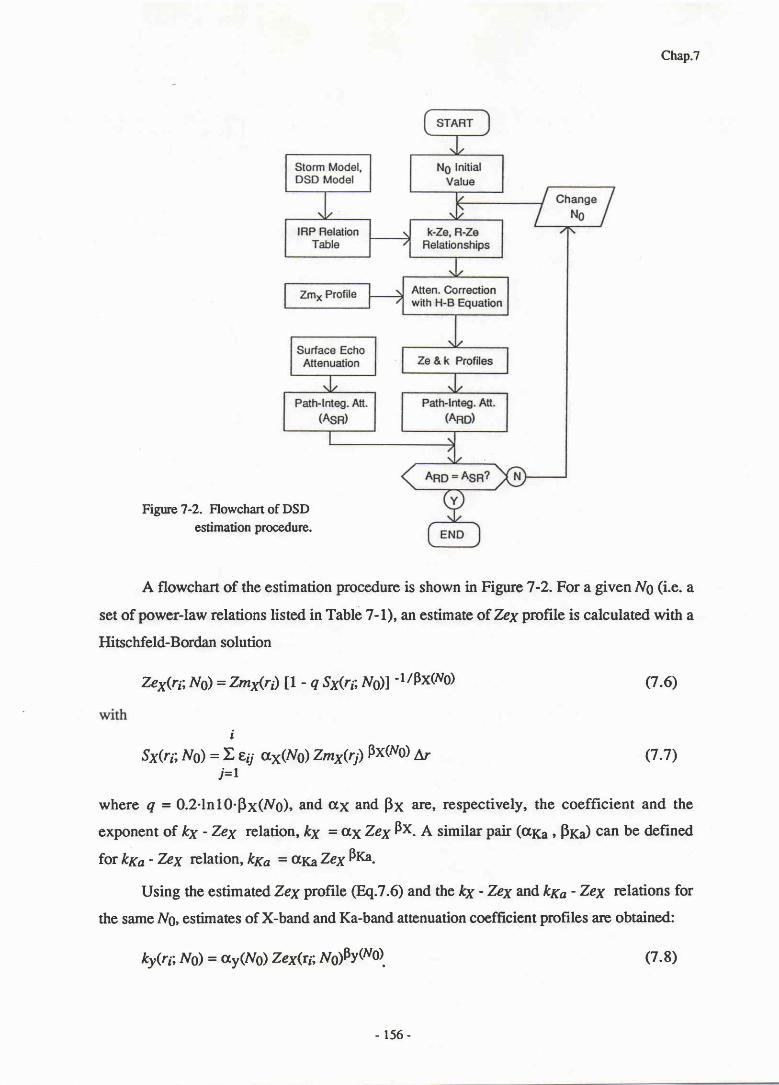
Chap.7
Figure 7-2. F"lowchart of DSDestimation procedure.
A flowchart of the estimation procedure is shown in Figure 7 -2. For a given Ng (i.e. a
set of power-law relations listed in Table 7-L), an estimate of Zelg profile is calculated with a
Hitschfeld-Bordan solution
ZeyQi;No) - Zm11{r) Il - qSx(ri; No)l -llFx@o)
i
Sx(r;; N0) - > Eij ax(No) Zmy(r) Fx(No) Ar
(7。6)
(7.7)j= l
where e = 0.2.1n10.p1(No), and c1 and p1 are, respectively, the coefficient and the
exponent of &y - Zex relation, &y - cr1 Zex Fx. a similar pair (ar" , FfJ can be defined
for kxa - Zex relation, /<5o = c[Ka Zey\rca.
Using the estimated Zex profile (8q.7.6) and the kx - Zex and kxa - Zex relations for
the same Ng, estimates of X-band and Ka-band attenuation coefficient profiles are obtained:
ky(r r;No) = cry(No) Zey(r;;Ns1FY0'rq
- 1 5 6 -
(7。8)
Chap.7
Estimates of X-band or Ka-band path-integrated attenuations are then
五υ,y=Σぅ(竹;均)△4ノ=1
ARD,! is known to be unstable when X-band radar wave is highly attenuateds). ttrus, we
force it equal to the surface echo-derived attenuation, A5p,y, and find a solution for Ng that
satisfies the equation
ARD,y=AsR,y。 (7。10)
Due to the fluctuation of surface scattering cross section (o0), AS*J is not accurate
when the path-attenuation is small. For example, it has been found from a statistical analysis
of surface returns in no-rain conditions that the standard deviation of surface d is 1 - 1.5 dB
for the flights used for the DSD estimation test. The same thing happens when path-
attenuation is so large that signal-to-noise ratio (S/N) becomes small. To avoid a noisy result
of the DSD estimation, the processing is done only when ASnJ is greater than 3 dB (2-way
path attenuation > 6 dB) and the effective S/N7) of the surface echo is greater than 6 dB. If
ASR,K' satisfies this criterion, it is employed for the processing (y = Ka in Eq.7.10). If not,
AsnX is then checked by means of the same criterion.
An approximate solution can be found by selecting a "best-fit" N0 from 13 Ng
candidates ranging from 1.4x10³ to 100x103 mm-lm-3 (see TableT-1). The maximum N0
error in this approximate solution is about fl.l dB. When the X-band path-attenuation is
negligible, this Ng errorcorresponds to about fr.z dB enor inApp,y. With increasing path-
attenuation, the error in App v increases for a given N6 error; however, the approximate Ng
solution has been found acceptable up to about 10-dB X-band Z-way path-attenuation,
corresponding to about 65 mm/h rain rate with a rain height of 3 km.
Once we obtain the Ng estimate, fg (the solution to Eq.7.10), we also have a set of
estimates of rain-parameter profiles including Zey, ky, and kKo,just by substituting fg into
Eqs. 7 .6 and 7.8. Similarly, profiles of the other DSD parameter, A, and rain rate (and any
other integral rain parameters) can be calculated with the corresponding power-law relations
(7.9)
( 7 。1 1 )
(7.12)
A(4;NO)=ζx(Wb)Z`x(rli;Ⅳo)ηXttD
R(■;No)=αx(ハb)Zgx(rぉⅣo)bXαθ).
157‐

Chap.7
It should be noted that rain rate can also be obtained from a k-R relation for fg or from an
integral of the product of drop water volume, drop terminal velocity and DSD over the
diameter D, and all the results should be consistent with one another. The same applies to any
rain parameter calculations, because all rain parameters are now mutually related in terms of
the DSD profile we have estimated.
7.1.3. Melting layer attenuation
In the above formulation, we have assumed that the hydrometeors along the path are all
raindrops having DSDs with a single Ng. Actually, however, other hydrometeors may exist.
In such cases, the modeling of DSD along the path and the calculation of path-integrated
attenuation from the Zmy profile requires modification. In the present analysis, wo use the
following scheme to incorporate the effect of non-liquid hydrometeors.
(1) For the processing of aircraft data, aZmprofile is classified into three regions; ice, melting
layer, and rain. For a stratiform rain in which a bright-band is evident from the Zrn profile, the
classification is relatively easy. In the case of other rain types, we make the classification
based on the 0"C isotherm height derived from the bright band observed at other stratiform
rains observed in the same flight.
(2) Radiowave attenuation in the ice region is negligible both at X and Ka-band-
(3) To evaluate the melting layer attenuation and k-Ze relations, wo assume that the melting
layer particles are spherical composite dielectrics and their DSD is given by a Nonbreakup-
and-Non-coalescence model8) (see Appendix 2.1). For stratiform rain, the thickness of the
melting layer is chosen to be 900 m (bright band Zm peak + 450 m), in which the particles
change their fractional volume content of water from 0.017 to 0.85 corresponding to wet to
watery snow 8). Since it has been found that ky - Zex and krca - Zex relations averaged over
the melting layer are close to those for rainfall, for simplicity, we use the same k-Ze relations
both for the rain region and the melting layer.
(4) In the case of convective rain, we assume that the particles start melting at 2-km above the
0"C isotherm height (i.e. "melting layer" for the convective rain is between 2-km above and
450-m below the 0"C height). This is based on an analysis of X- and Ka-bandZm profiles of
heavy convective storms observed in the flight on November 1, 1988, which indicates that
Ka-band radiowave starts attenuating around 2-lan above the estimated 0"C isotherm height.
This model is clearly too simple to represent the physical phenomena above the 0"C height in
-158-

Chap.7
the convective storrn. In this region, attenuation may be caused by wet growth of ice or snow
and supercooled raindrops; dense water cloud can also cause a significant Ka-band attenuation
in some cases. Therefore, k-Ze relations for this region may not be the same as those for rain.
Depending on the convective activity, the rain top height may also differ from case to case.
Such a detailed convective storm modeling is beyond the scope of the present study. lnstead,
we will evaluate the effect of storm modeling on the Ng estimate by comparing the results
obtained with the above simple convective model and those with the stratiform model that
assumes the melting layer thickness of 900 m (OoC isotherm height t 450 m).
(5) In any case, the "path-averaged" rain rate shown later is defined as the average over the
rain region only. T'he Zm values of the melting layer are used only to evaluate the attenuation
of radiowaves passing through them.
The storm model used here is illustrated in Figure 7-3.
: . : . : ' : . : . : t ce . : . : - : - : . :H+2
km
H- .45km
H+.45
Convective model Stratiform model
Figure 7-3. Storm model used to calculate path-arenuation
and path-averaged rain rate frcmZnz profile.
- 1 5 9 -
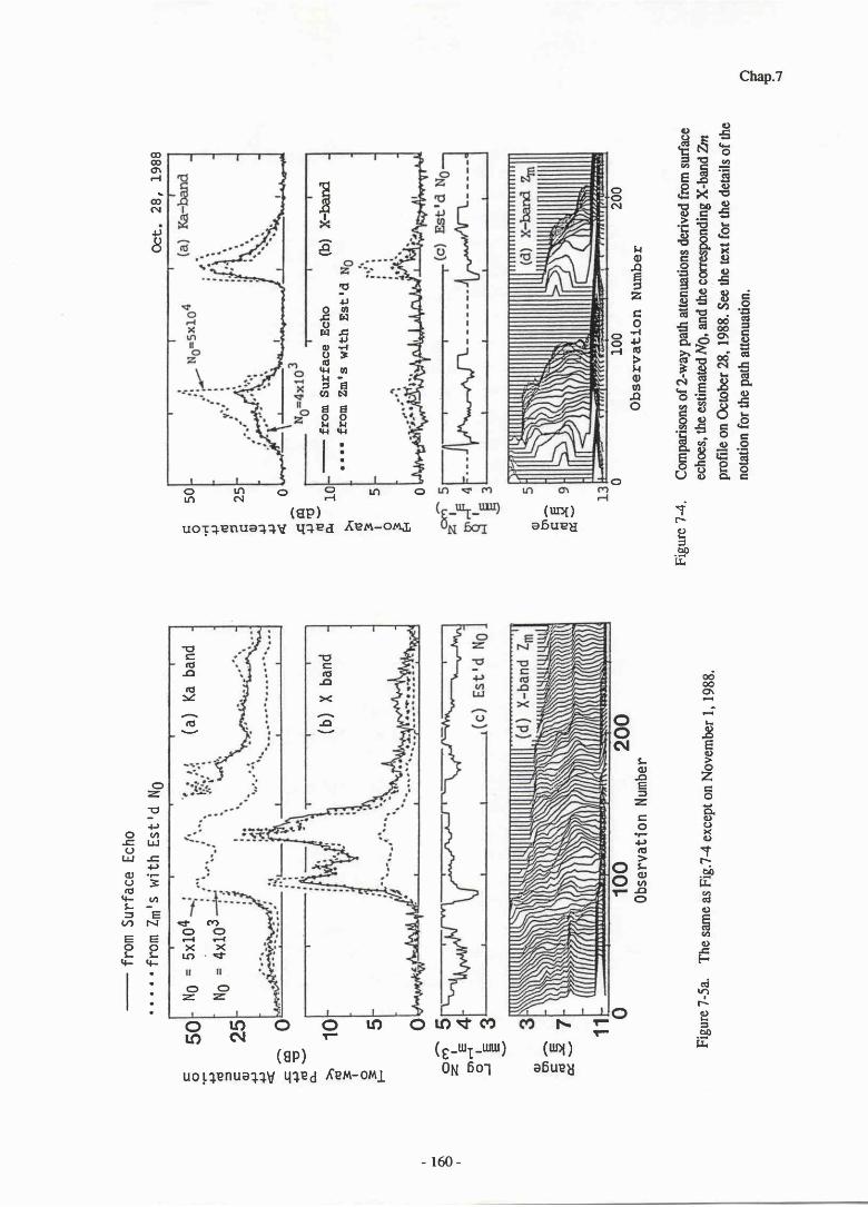
fro
m S
urf
ac
e E
ch
o'.
...f
rom
Z
m's
wit
h E
st'
d
Ng Ns
N0
( “ 0 )
に 0 中 一 ● コ C O ´ 一 く 〓 ↓ 0 」 、 ● 〓 ‐ 0 〓 ト
50
25 0
・0 5 0
( m O )
口 O H J “ , C O J J く 〓 J “ 餞 、 C 〓 1 0 3 自
( ∞ ‐ E H ‥ E E ) ( E 〓 )
O Z 0 0 コ 0 い E ● ∝
5。
25 0
‐0 5 0 5 4 3
4 3
0 0
X X
5
・ 4
(a)
Ka
ba
nd
上 8 ‐
(b)
X b
an
d
7 11 0
10
0
20
0O
bs
erv
ati
on
Nu
mb
er
fro
m
Su
rfa
ce
Ech
orr
rr
f16
m
Zm
rS
Wlt
h
ES
ttd
(b)
x-ba
rd
0
10
0
20
0O
bs
erv
atl
on
N
um
be
r
Com
paris
ons of
Z-w
ay pa
th at
tenu
atio
ns
deriv
ed from
sur
face
echo
es, th
e est
imat
ed lV6,
and t
he co
nesp
ondi
ng
X-b
an d7
npr
ofile
on
Oco
ber 2
8, 1
988.
See
the t
ext f
or th
e de
tails
of rh
eno
tatio
n for
the
path
atre
nuat
ion.
o $^
CE
dJ
1&
-
Fig
ure
7-4
.
O F も ヽ
Oc
t.
28
, 1
98
8
Fig
ure
7-5
a.
Th
e sa
me
as F
ig.T
-4 exc
ep
t on
No
vem
be
r l, l9
gg
.

Chap.7
OO∞
e一coo)
おいよ
2一¨直
L00E5Z C〇一一“>LO∽OO
OON
OOr
8R09L00(8P)
uo1lonuollv Ч 12d κOM-OM上
Ю 寸 ∞ ∞ ト
(8-ШI―ШШ) (Ш】)
ON 6ol o6u口と
rr
OC●0 一〉 (0)
-161-
Chap。7
7.2 Results and Discussion
The DSD estimation is tested using the data obtained from the flights over the Atlantic
Ocean on October 28 and November 1, 1988. The storms observed on the former date were
localized convective cells, while on the latter date, mixed convective and stratiform rains were
observed.
7.2.1 Spatial trend of N0
Results of path-averaged Ng estimation are shown in Figures 7-4 and 7-5. In the
figures, the plots labeled (a) and (b) represent the Z-way path attenuations at Ka-band and X-
band, respectively. The curves in (a) and O) include: the attenuation derived from the surface
echo; the value obtained by selecting the best NO (NO); and values obtained by using frxed Ng
values of 5x10⁴ and 4x103 mm-lm-3, for a guideline of upper and lower boundaries of Ng
naturally found. These limits are selected based on a statistical analysis of disdrometer data at
Kashima, and represent the lO Vo and 90 Vo ranges of the distributions of Ng values. The
estimated Ng's are shown in (c). To provide a qualitative indication of the storm structure, the
X-band Zm profrle versus range from the aircraft is shown in (d).
It is found that Ng is almost everywhere bounded by the two extremes (5x10⁴ and
4xIO3 mm-lm-3) suggesting that the estimation procedure gives reasonable results. The data
also show that fg undergoes gradual spatial variations that are probably caused by internal
storrn structure. It is also found that a sharp spike in fg sometimes appears at the edge of an
intense region. This phenomenon might be related to DSD properties specific to the storm
edge or to the partial beam filling9-ll). Although the -3 dB beamwidths of X and Ka-band
antennas are almost the same, a slight misalignment of antenna direction or a small difference
in antenna patterns may also be a problem at the storrn edge.
For the heavy convective rains, the Ng estimation is also made using the stratiform
model as mentioned in Section 7.1.3. The fg'r are found to be 0 - 2 dB (about 1 dB on
average) larger than those using the convective model. Although the difference is small
compared with the variability in natural N6's and comparable in magnitude to the errors due to
other causes (described later), more study of the convective storrn structure is required to
improve the accuracy in the Ng estimation.
162-
Chap.7
7.2.2 Consistency with Ka-band Ze
In order to further evaluate the validity of the estimated N0, we make a consistency
check using ZmKa profile that is independent of the DSD estimation. The ZmKo profile is
converted to aZeyoprofile by making the attenuation correction
盈κα(■)=ZZKa(■ )eXp[0.21n10 Aκα(■;lMo)]
with
( 7 . 1 3 )
(7.14)
(7.15)
:
AKa(■;No)=Σ εヴ場ζα(竹;″b)△r
ノ=1
00KaWO)Zgx(■;島)βKa蘭).堵α(rli;」Mo)=|
We analyznhere only the data for whichNo is derived by using the Ka-band surface echo
attenuation, since the fg thus obtained guarantees an excellent stability in the attenuation
correction for Ka-band Zm's.
- Ratio of Ka-band Ze to X-band Ze :
Since ZeKo is subject to larger Mie scattering effects than Zex, the ratio of Zeyoto Zey
depends on DSD. The Ka/XZe ratro obtained from the measured (and attenuation corrected)
Zds should be consistent with the estimated fg value. Examples of Zm andZe profiles for
three differentf6s are shown in Figure 7-67).TheZeyandZe1ain this figure are calculated
with W.7.6 (lettingN0 =Ng) and Eq.].13, respectively. The profile (a) is obtained from the
October 28 flight. In this case, Ng is 8000 mm-lm-3. The other two, (b) and (c), are obtained
from the November 1 flight and have, respectively, large and smafl ̂ [g's. As shown in Figure
7 -6, the WX Ze raio in the rain region appears to change from case to case.
Figure 7-7 shows the scattergram between path-averaged Ze ratio (ZeR^sas) and Fg for
tight to moderate rain rate region shown in Figure 7-5, during which Ka-band path-attenuation
is available from the surface echo (Observation number 200 - 330 in Figure 7-5b). The
ZeRono, is calculated from the equation
Z沢 ″ α∫〓1ル Σ EZg施(■;島 )/盈 x(4;島 )]j=1
(7.16)
where the summation from i = 1 to n extends only over those n gates that span the rain region.
Also shown in the figure are theoretical curves assuming the exponential DSD model
-163‐
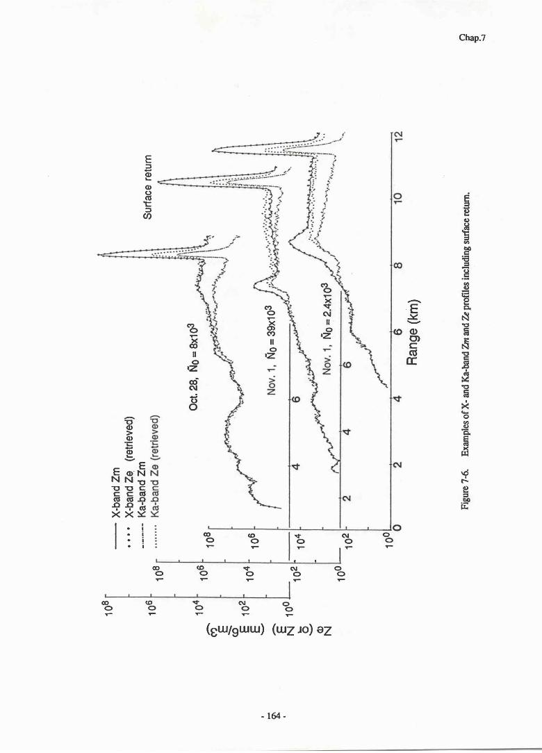
8 6
0 0
X-b
an
d
Zm
o .' o
X-b
an
d
Zq
(re
trle
ved
)K
a-b
an
d
Zm
Su
rfa
ce re
turn
04
02
00
δ E お E E ) ( E N 』 3 o N
ム T ‐
10
8
10
6
10
4
rcz
10
0. to
o
-10
208
06
Oct
. 29,
NO
= 8
x103 6
Ra
ng
e (km
)
t oob
O F ” ● ‘一
雨0=39x103
山0=2。
4x10³
Fig
ure 7
-6.
Exa
mpl
es
of X
- and
lG-b
and7
ntnd
Ze p
rofil
es incl
udin
g surf
ace re
turn
.

Chap.7
for givenZey's which correspond approximately to the values observed in the same period.
For larger Ng's (logrO NO ) 4) and smaller Ng's (logrO NO S 4), path-averaged Zey's are
found to be about 30 dBZ and 37 dBZ, respectively. The theoretical value (ZeRsslc) is
obtained as follows: By specifyingZexandNg, an exponential DSD is uniquely determined.
With this DSD,Zeya and then ZeRsaly is calculated
We can see that ZeRynsas is consistent with ZeRgals, although ttre former is somewhat
smaller at the small Ng range. This discrepancy might be caused by the deparnre of natural
DSD from the exponential shape. Note that the two large ZeRpraojs (: 3.8 dB) at loglg N0 =
5.0, shown in Figure '7-7, are obtained at the very sharp storrn edge (Observation number =
225 n Figure 7-5b), suggesting the existence of a non-uniform beam filling effecr
- Comparisons of rain rates dcrived by different methods :
The other way to check the validity of the ilg estimate is to examine the consistency
between rain rates calculated from X- and Ka-band Ze's. We compare three different rain rate
estimates; a rain rate derived from Zex with I7o (Rzr), that derived from ZeKo with fg
(Rz*,oS2r), and that derived from ZeKo assuming the MP distribution (Rzk,up). RTis
defined by Eq.7.12, while the latter two are given by
(mこo一お∝①NX鶯Y
3
2
1
0
1
‐2
‐3
‐4
3 3.4 3。6 3 . 8 4 4.2 4.4
Log10 NO
4.6 4.8
Figtrre 7-7. Scauergram of the ratio of retrieved Ka-band 7z n X-band k (KaIXZz
ratio) versus estimated Ng value (N0).
X-band ze =go dBz g o'Y -v -
l'--- 8- ^ oUjrre-g-E
165‐
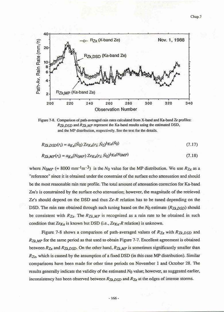
4。
2。
1。
8
6
4
2
FヽEE)2c匡
Ec匡
ゞく止ta
320 340
Chap.7
(7.r7)
(7.18)
2 0 0 220 240 260 280 300
Observation Number
Figure 7-8. Comparison of pattr-averaged rain rates calculated from X-band and Ka-bandk profiles:RZ*,OSO and R71r,p,4p represent the Ka-band results using tlre estimated DSD,
and the MP distribution, respectively. See the text for ttre details.
Rzρ sD(■)=gκ aWo)盈 施(■;均 )bttCNO)
Rz*Up(ri) = axa(Noup) ZeyaQ;; fldbxa@oup)
where Nour (= 8000 mm-tm-3) is the Ng value for the MP distribution. We use Rzr as a
"reference" since it is obtained under the constraint of the surface echo attenuation and should
be the most reasonable rain rate profile. The total amount of attenuation correction for Ka-band
Zm's is constrained by the surface echo attenuation; however, the magnitude of the retrieved
Ze's should depend on the DSD and thus Ze-R relation has to be tuned depending on the
DSD. The rain rate obtained through such tuning based on theNg estimate (RV2pSD) should
be consistent with Rzr. The Ryp,Mp is recognized as a rain rate to be obtained in such
condition that ZeKo is known but DSD (i.e., ZeKs-R relation) is unknown.
Figure 7-8 shows a comparison of path-averaged values of R7 with RTa,pgp and
Rz*,tt1p for the same period as that used to obtain Figure 7 -7 . Excellent agreement is obtained
between R7 and Rm,pSo. On the other hand, Rz*JrIp is sometimes significantly smaller than
R7s, which is caused by the assumption of a fixed DSD (in this case MP distribution). Similar
comparisons have been made for other time periods on November 1 and October 28. The
results generally indicate the validity of the estimated Ng value; however, as suggested earlier,
inconsistency has been observed between Rz*pSo and R7* at the edges of intense storrns.
-o- R1 (X-bandZe) Nov. 1 , 1988
RZk,DSD (Ka-bandZel
- 166-
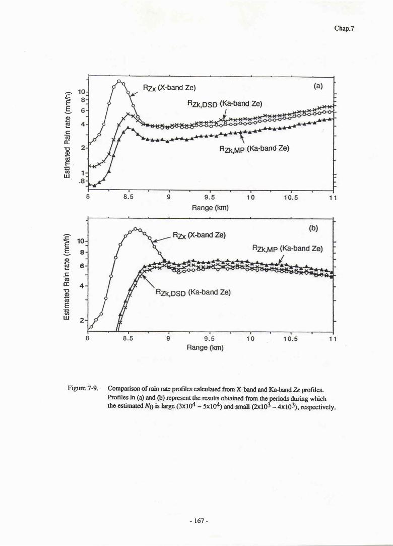
Chap.7
(∈EE)2E
ct匡
09cE一ちШ
・0 8
6
4 2
(ξEE)2“』c一“匡
02“E一覇Ш
Fi即 7‐9. Comparison ofrain ra“ prorlles calculated■om X―band and Ka‐bandia pЮ rlles.
Pro■les in cal and O)representthe resuls obtaind from ale periods duttng whichthe csdmated数)おlargc(3x10⁴~5x10⁴)and smal1 0X103~4x10³),respecdvely.
Rzx(X‐ band ze)
RZk,DSD (Ka-band Ze)
Rzk,MP(Ka‐ band Ze)
R孜 o(‐band ze)
‐167-
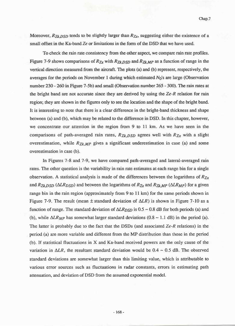
Chap.7
Moreover, Rvrp56r tends to be slightly larger than RZr, suggesting either the existence of a
small offset in the Ka-band Ze or limitations in the form of the DSD that we have used.
To check the rain rate consistency from the other aspect, we compare rain rate profiles.
Figure 7-9 shows comparisons of Ry*with Rz*DSoandRVr,Mp as a function of range in the
vertical direction measured from the aircraft. The plots (a) and (b) represent, respectively, the
averages for the periods on November I during which estimated Ng's are large (Observation
number 23O - zffi n Figure 7-5b) and small (Observation number 265 - 300). The rain rates at
the bright band are not accurate since they are derived by using the Ze-R relation for rain
region; they are shown in the figures only to see the location and the shape of the bright band.
It is interesting to note that there is a clear difference in the bright-band thickness and shape
between (a) and (b), which may be related to the difference in DSD. In this chapter, however,
we concentrate our attention in the region from 9 to 11 km. As we have seen in the
comparisons of path-averaged rain rates, Rzk,DSD agrees well with Rzx with a slight
overestimation, while Rzk,Mp gives a significant underestimation in case (a) and some
overestimation in case (b).
In Figures 7-8 andT-9, we have compared path-averaged and lateral-averaged rain
rates. The other question is the variability in rain rate estimates at each range bin for a single
observation. A statistical analysis is made of the differences between the logarithms of R7,
and RTI,DSD (Al.,Rosp) and between the logarithms of R7- and Rvayp (MRuil for a given
range bin in the rain region (approximately from 9 to 11 km) for the same periods shown in
Figure 7-9. The result (mean t standard deviation of ALR) is shown in Figure 7-lO as a
function of range. The standard deviation of MRoso is 0.5 - 0.8 dB for both periods (a) and
(b), while MRyp has somewhat larger standard deviations (0.8 - 1.1 dB) in the period (a).
The latter is probably due to the fact that the DSDs (and associated Ze-R relations) in the
period (a) are more variable and different from the MP distribution than those in the period
(b). If statistical fluctuations in X and Ka-band received powers are the only cause of the
variation in ALR, the resultant standard deviation would be 0.4 - 0.5 dB. The observed
standard deviations are somewhat larger than this limiting value, which is attributable to
various error sources such as fluctuations in radar constants, errors in estimating path
attenuation, and deviation of DSD from the assumed exponential model.
168 -
Poriod(a)△
LRDSD
( m O ) ∽ Φ 一 ” 」 c 一 ” 匡 O Φ “ ” F 二 雨 Ш 一 〇 〇 0 コ 。 0 , C 一 〇 O C O 』 0 〓 一 〇
‐ い い つ ‐
9.8
1
0
10
.2
10
.4
10
.0
10
.8R
an
ge
(km
)
9。6 9。0 10 10。2 10。4 10.6 10。8
Range(km)
4 3 2 1 0
●1
・2 4 3 2 1 0
●1
・2
9。8 10 10。2 10。4 10.6 10.8
Range(km)
9.8 10 10.2 10。4 10.6
Range(km)
9。4
Fig
ure 7
-10.
Diff
eren
ces b
etw
een th
e lo
gari
thm
s of R
21 a
nd R7p
5p
(Aln
p5p)
an
d ber
wee
nth
e lo
gari
thm
s of R
21 a
nd RV
l,yp
(MR
Uil
as a
func
tion o
f ran
ge fo
r the
sam
epe
riod
s (a)
and
(b) s
how
n in
Fig
.7-9
. In tt
re fig
ure,
solid
curv
es re
pres
enr th
e mea
nof
the d
iffer
ence
and v
ertic
al ba
n in
dica
te th
e mea
n t s
unda
rd de
viat
ion.
の コ ” ● 』
Pe
rio
d (b
) A
LH
oso
PenOd(b)△
LRMP
Chap.7
7.2.3 Error sources
There are a number of uncertainties relating to the dual-parameter radar measurement.
Some factors important for this method are summarized below.
- Surface scattering cross section (d): Temporal and spatial variation in d is a majorerror
source in estimating path-attenuation from surface return. It is known that over ocean, o0
depends strongly on surface wind condition (speed and direction) for intermediate to large
incidence angles (> 15"). For near-nadir incidence, the wind dependence of d is relatively
small and becomes minimum around incidence angles of 8 - 10" 12). Another source of error
is the potential effect of raindrop striking on the sea surface scattering properties. This effect
has been observed at la.rge incidence angles 13'14). Although no measurement on this effect
has been reported for near-nadir incidence cases, it may be relatively small because of the
dominant contribution of specular scattering component to d. In the experiment conducted in
the fall 1988, measurement was made at incidence angles around 7 degrees, at which o0 is
expected to depend on the wind condition only slightly. This might be a reason for the
relatively small standard deviation (1 - 1.5 dB) of surface returns we have observed in no-rain
condition. Nevertheless, variability in cil caused by environmental conditions such as wind,
long gravity waves and the raindrop striking should be studied more to assess the accuracy in
path-attenuation estimation from surface return. Over land, the use of surface return is more
problematic than over ocean because of the larger spatial variability in o0. One way to reduce
the errors is to use the difference of path-attenuation estimates at two frequencies instead of the
estimate from a single frequency 15).
- Bright band and convective storm modeling: As mentioned in Section7.2.1, errors in
estimating the attenuation caused by hydrometeors at and above the bright band or 0"C
isotherm height can cause non-negligible errors in estimating the DSD and other rain
parameters. For stratiform rain, refinement of the bright band model would be required. For
example, Figure 7-9 indicates that the bright band thickness depends on DSD and probably
other precipitation properties as well, while the present model assumes a constant thickness of
900 m. The modeling of convective storrn may be more difficult than the modeling of
strariform rain; unlike the stratiform rain, it is difficult to distinguish the hydrometeor phase
state from the radar reflectivity profile especially when only a single-frequency, non-
polarimetric radar is available. However, further analyses of the aircraft data may provide
statistical models which depend upon storrn intensity, vertical reflectivity profile, oE.
170 -

Chap.7
- Non-uniform beamftlling: It has been observed in the present study, that the Ng estimates
sometimes show a positive or negative peak at the edge of an intense storrn. This suggests the
existence of errors due to the horizontal non-uniformity in rainfall within a radar resolution
volume. Since the error caused by the non-uniformity is larger in the path-attenuation (or rain
rate) estimate from the surface return than the rain rate estimate from the radar reflectivity 9't01,
the dual-parameter methods employing the surface return may not be applicable to the storm
edge or to rain cells having smaller horizontal sizes than the radar foot print sizel l).
Conversely, it may be possible to detect the existence of partial beam filling by examining the
spatial uend of estimated DSD parameters.
7.2.4 Effects of errors in Zm and Af,& on N0 estimation
Errors in Zm measurement and Agp estimation cause the error in the path-averaged Ng
estimation. In this section, we make a simple error analysis for the case where the DSD is
uniform over the path. We also assume that X-band path attenuation is negligible (Zmy =
Zefl and that Zex and kxa are proportional to 6th and 4th moments of DSD. These
assumptions approximately hold for the stratiform rains that we have analyznd in section
7 .2.2.In this case, the Ng estimate is given by
No l -F -CASn ,Ka /ZeyF , F=5 /7 (7 .19 )
where ASnKo - (n'A,r) krca. For convenience, wo consider the errors in the logarithms of
measured and estimated quantities. Irtting (J = 10.log1gN9,X -- 10.1o910.4 SR,Ka, and I =
l0.logrcZey, Eq.7. 19 is expressed as
u - Io/(l-p) logc + r/(r-Fl x - p/(l-F) r. Q.zo)
By expressing X and I as X --XO +x and Y :YO +y where Xg and Yg are true values, and
x and y are corresponding errors, the error in U, u, becomes
“=1/(1-β)χ―β/(1-β)y (7 .21)
where C is assumed to have no error. Assuming that x and y are independent random
variables with mean values of xandy and standarddeviations of o* andoy, rospoctively, ttre
mean and variance of u (ii and ou2, respectively) are
- 17r

所=1ズ1-β)ヌーp/(1-β),
Chap.7
(7.22)
(7 .23)ou2 = llQ-F)z axz + $211t-9>2 of .
Statistical fluctuation in radar received power is the major cause of the variation in Y. This
contributes also to the variation in X; however, the major part of the variation is caused by the
fluctuation in surface d. Since the number of independent samples averaged (logarithmically
in this system) is 128, oy = 5.57 /"m = O.49.In order to estimote o1, attenuated surface
returns have been simulated by using Ka-band surface returns measured in no-rain condition
subtracted by the sum of a constant attenuation and a received power fluctuation term
approximated by a Gaussian noise having the standard deviation equal to oy. It has been
found from a statistical analysis of this simulated data set that o* is 0.2 - 0.6 for ASR,K' - 15
- 5 dB (Z-way path attenuation 30 - 10 dB). Using these estimates of o* and oy, ou becomes
1.4 - 2.4. If we assume that i = 0 and y = I dB (the latter represents the X-band radar
calibration error), u = 2.5 dB. These errors are not negligible; however, they are still much
smaller than the total variability in lO-logNg that ranges approximately from 30 to 50 (Ng =
103 - 105).
The calibration error in the Ka-band radar does not affect the Ng estimate but does the
resultof theconsistencycheck. Forexample, theKa/XZeratio showninFigure 7-7 is offset
by the same factor as a bias error inZmga (in dB unit); however, the loglgNg dependence of
the Ze ratio is still consistent with the theory in a relative sense. Similarly, a bias error in Zmyo
simply causes an offset in the logarithm of R7p,p5p and RZk,Mp shown in Figures 7-8
through 7-lO. That is, Rv2,74p is still inconsistent with the reference rain rate R7., because the
difference between R71r,114p and R7, which has both positive and negative values depending
on the period, cannot be explained by an offset in Z.rnya.
7.3 Conclusions
We have shown test results of a dual-parameter rainfall measurement for a down-
looking airborne or spaceborne radar, which combines a reflectivity profile and a path-
integrated attenuation. It has been found that the values and the spatial trend of the path-
averaged DSD parameter, Ng, estimated from the experimental data a"re reasonable and that
they are consistent with the measured Ka-band reflectivity which is independent of the Ng
estimation. These results indicate the feasibility of estimating DSD parameters from space. The
r72 -
Chap.7
DSD information provided from this method would lead to more accurate rainfall
measurements and a deeper understanding of precipitation processes. It also has a potential to
improve a wide range of radar rain measurements. For example, DSD properties and
associated Ze-R relations (and other IRP relations) obtained at a part of a storm could also be
apptied to other part of the storm where path-attenuation data is difficult to obtain. Applying
this method to spaceborne radar measurements with global coverage would extend our
knowledge of the dependences of Ze-R relation on rain type, geographical location and
synoptic conditions.
More studies are required to clarify uncertainties such as the raindrop striking effect on
o0 and non-uniform beam filling. Although the storrn models used in this study should be
adequate as a first-order approximation, refinements in the bright band and convective storrn
models are required to improve the accuracy in estimating the attenuation due to non-liquid
hydrometeors aloft. Using a gamma DSD model instead of the exponential model and
incorporating storm-type and height dependences of the DSD model should also improve
rainfall retrieval accuracy. In the aircraft experiment, multi-frequency radiometer data as well
as the radar data were obtained. The DSD estimation is also possible by combining the radar
and radiometer data instead of using the surface return. Combining such multiple sensor data
would also be useful to develop the improved storm model and to achieve better rainfall
retrievals.
r73 -
Chap.7
References
(1) Kozu, T., R. Meneghini, W. C. Boncyk, K. Nakamura, and T. T- Wilheit, 1989:
Airborne radar and radiometer experiment for quantitative remote measurements
of rain. Proc. GARSS89, Vancouver, Canada, L499-I502.
(2) _, K. Nakamura, and R. Meneghini, 1991: Estimation of raindrop size distri-
bution parameters from a dual-parameter spaceborne radar measurement. Pneprints,
25th Conf. Radar Meteor., Paris, Amer. Meteor. Soc., 384-387.
(3) _, _, _, and W.C. Boncyk, 1991: Dual-parameter radar rainfall
measurement from space: A test result from an aircraft experiment
IEEE Trans.Geosci. and Remote Sens., GE-29, 690-703.
(4) Fujita, M., 1983: An algorithm for estimating rain rate by a dual-frequency radar.
Radio Sci., L8, 697 -708.
(5) Hitschfeld, W. and J. Bordan, L954: Errors inherent in the radar measurement
of rainfall at attenuating wavelengths. J. Meteorol.,ll, 58-67 .
(6) Meneghini, R. and K. Nakamura, 1990: Range profiling of the rain rate by an airborne
weather radar. Remote Sens. Environ,3l, t93-209.
(7) Meneghini, R. and T. Kozu, 1990: Spaceborne weather radar. Artech House, Boston.
(8) Awaka, J., Y. Furuhama, M. Hoshiyama, and A. Nishitsuji, 1985: Model calculations
of scanering properties of spherical bright-band particles made of composite dielecrics.
J. Radio Res. Lab.,32,73-87.(9) Nakamuffi, K., 1989: A comparison of the rain retrievals by backscattering
measurement and attenuation measurement. Preprints ,24th Conf. Radar Meteorol.,
Tallahassee, FL, Amer. Meteor. Soc., 689-692.(10) Amayenc, P., M. Marzoug and J. Testud, 1989: Non uniform beam filling effects
in measurements of rainfall rate from a spaceborne radar. ibid,569-572.
(11) _, and _, 1990: Analysis of cross-beam resolution effects in rainfall
rate profile retrieval from a spaceborne radar. Proc. GARSS'90, College Park, MD,
433-436.(12) Masuko, H., K. Okamoto, M. Shimada and S. Niwa, 1986: Measurement of
microwave backscattering signatures of the ocean surface using X band and Ka band
airborne scatterometers", J. Geophys. Res.,91, (C11), 13065-13083.
(13) Moore, R.K., Y.S. Yu, A.K. Fung, D. Kaneko, G.J. Dome, and R.E. Werp, L979:
Preliminary study of rain effects on radar scattering from water surfaces.
IEEE J. Oceanic Eng., OE-4, 3I-32.
(14) Bliven, L.F- and G. Norcross, 1988: Effects of rainfall on scatterometer derived wind
speeds. Proc. 1GARSS88, Edinburgh, UK, 565-566-
(15) Meneghini, R., J.A. Jones and L. H. Gesell, 1987: Analysis of a dual-wavelength
surface reference radar technique. IEEE Trans.Geosci. and Remote Sens.,
GE-25, 456-471.
‐174-
Chap.8
CHAPTER 8。 CONSIDERATION OF RADAR RAINFALL RETRIEVAL
ALGOR「 HMS FROM SPACE
In this chapter, we consider algorithms to estimate rainfall parameters from a TRMM
type spaceborne single-frequency radat, operated with a multi-frequency microwave radio-
meter and a visible/infrared radiometer. This is followed by a consideration of usefulness of
the DSD estimation method we have studied in this thesis for the spaceborne radar rainfall
measuremenL
As described in Chapter 1, the strategy to estimate rainfall parameters depends on the
resolution (both temporal and spatial) and accurzrcy requirements. Utilizing statistical properties
of rainfall such as lognormal or gamma rainfall distribution function and a statistical correlation
between area-integrated rain rate versus raining area for convective storms has been found to
be useful to estimate low resolution rainfalt parameters under limited measurement capabilities.
While the low resolution rainfall estimates are sufficient for many climatological studies,
high resolution rainfall parameter estimation is essential for various local to mesoscale
mereorological and hydrological studies. The high resolution rainfall information is also
important for applications such as short-term weather forecast and flood warning. It is also
necessary to develop and to refine various statistical and climatological methods for estimating
low resolution rain parameters. The consideration in this chapter is, therefore, concentrated on
the rainfall retrieval with the high resolution (every observatioll - one raining area).
8. 1 Estimating Apparent Effective Radar Reflectivity Factor (Zm)
As discussed in Chapter 2, the radar rainfall retrieval begins with obtaining the apparent
effective reflectiviry factor (Zm), which can be derived from the radar equation neglecting rain
attenuation. For the surface return, "apparent" normalized surface scattering cross section,
d^, will be calculated simitarly. It is important to generate oo,n as well asZm, because: (1)
For the algorithms using the surface return level, the data outside the rain region is essential to
extract the path-attenuation; (2) from the d* measurement over the ocean, surface wind speed
can be estimated; (3) a world wide surface scattering cross section map will be useful for
future remote sensing of Earth surface from space.
Since Zm and,o0- are the quantities obtainable from only the instrument dependent
175

Chap.8
parameters, they can be derived in a straightforward manner. Therefore, they are suitable as
"I-evel 1" products generated from "Irvel 0" product (original count value sent from the
satellite with some ancillary data added). It should be noted that the radar calibration (both
internal and external) is the most important task to assure the accuracy of those quantities. In
this stage, several additional processing should be done: (1) geometrical information, e.g. the
positions of the satellite and the center of a surface FOV, will be added to the product for each
observation; (2) "bad" data, e.g. observations during a satellite maneuver or radar transminer
turn-off should be rejected; (3) in order to extract the signal power from the measured (signal +
noise) power, an independent noise level monitoring and a noise level subraction are required.
- Radar calibruion
To assure the accuracy of Zm and op,rr, both internal and external calibration schemes
are to be employed The internal calibration includes: the periodical monitoring of the transmit
power, and the total noise power of the receiver output when the receiver sees a stable internal
terminator or a stable land background temperature, which provides a measure of the short-
term variation in the receiver gain; and the measurement of receiver input-output transfer
function using an internal signal generator which may be done on a weekly basis.
In addition to the internal calibration, external calibration is required to calibrate the
radar as a whole. One useful methd is to use a radar receiver and a beacon transmitter to
calibrate "forward" and "backward" paths of the radar signal including antenna characteristics.
The beacon transmitter, if it is arrayed with appropriate separation in space, could provide the
transfer function of the backward path of the radar. The overall system gain can be calibrated
by using an artificial reference target on the ground such as corner reflectors. In the case of
down-looking spaceborne radar, however, the return signal from such a r:eference point target
may be masked by strong surface clutter. Active radar transponders with some delay circuit
would be necessary to provide sufficient scattering cross section and to separate the return
signal from the ground clutter. It may also be a good scheme to use wide homogeneous
surface targets such as sea surface and tropical rain forests to calibrate the radar, although it
would be necessary to check the d value of such areas and its uniformity periodically by other
means.
The most direct rain radar calibration would be to use rain itself as a reference, as we
have tried in the T-3g experiment. The rain measurement on the ground may be made with
raingages, disdrometers, gtound-based radars, and micro- or millimeter wave links. The
176-
Chap.8
success of the "rainfall" method depends on how "good" rain can be observed simultaneously
by the ground-based and spaceborne sensors; the chance to conduct it may not be frequent.
Nevertheless, once we have several such data sets, they should be very useful to calibrate the
radar externally. The advantage of this methd is that the radar equation same as that for the
actual rain observation is used. An extension of this method is an adjustment of a radar
constant based on the radar reflectivity and rain rate statisticsl'2). Since this scheme does not
necessarily require simultaneous measurements, it can be conducted widely by using existing
rainfall measurement facilities over the world. This scheme, as necessity, requires a long
integration time and therefore the temporal resolution of the calibration is poor.
One uncertainty in comparing the rain rates as measured by ground-based and by
spaceborne radar is Ze-R relationship to be employed. If Ze-R relation is biased, the resultant
system calibration constant is also biased. Accordingly, the use of such system constant would
cause bias errors in rain rate estimation at other locations. During the calibration period,
therefore, DSD measurement should be performed at the calibration site to relax such bias
errors. Non-uniform beam filling within a radar resolution volume, which is another cause of
the bias error, should be taken into consideration as well.
8.2 Estimating Rain Rate and Liquid Water Content
The general concept of rainfall retrieval is to estimate various rainfall parameters of
interest from the radar measurables. From the single frequency spacebonre radar, we can
expect the following measurables; Zm profrle, surface return, ffid miror image Zm ptofile-
Although the mirror image may be used to estimate path-attenuation combined with the "direct"
image, we concentrate the discussion on the former two. The use of the miror image is a
subject of fufure study. We consider here the processing of l-evel 1 products (Zm and o0,n) to
rain rate and LWC profiles for each observation (Irvel 2 products). In addition, estimation of
several DSD related quantities useful to improve the rainfall retrieval is discussed.
8.2.1 Z-R and Z-W methods
The conventional way to estimate rain rate, R, has been to use an empirical power-law
Z-R or Ze-R relationship (for convenience, we call this type of method "Z-R" method even if
the quantity Ze is employed instead of Z);
Ze = cr RF.
t77 -
(8.1)
Chap.8
An extension of this scheme is to adjust the coefficients (a,F) based on the past experience of
rain-type or climatological dependences of the coefficients. The other extension is to use more
general relationships between Ze andR, e.g., piece-wise regression lines for different rain rate
ranges, since a single power law may not fit well over the total rain rate range. To establish
such aZe-R relation data base requires a comprehensive survey of past measurements over the
world. Disdrometer data that have been collected at many locations in mid-latitudes and at
several tropical sircs3'4) should be useful to study the properties of DSD; dependences on rain
type, season, and climatological regimes. DSD properties and associated Ze-R relations of
oceanic rainfall are poorly known, ffid have to be studied with airborne or shipborne sensors.
When rain attenuation up to a radar scattering volume is not negligible (2 or 3 dB or
more), rain attenuation correction is required. The attenuation can be estimated in a similar
manner to the Z-P- method; using an empirical k-Ze relationship, k being a rain attenuation
coefficient (usually in dBlkm). If the attenuation becomes large (-5 dB or more), such an
attenuation correction is known to be very unstable.
To estimate liquid water content 6WC; U/), the same scheme, Z-W method, may be
employed; however, the correlation betweenZe andW is worse than that betwennZe andR-
Therefore, the Z-W method would be very erroneous unless a large amount of averaging is
employed, and some dual-parameter methods would be necessary.
8.2.2 Surface Refgrence Target (SRT) method
A total path attenuation can be deduced from the surface return measuremenl Since the
microwave attenuation coefficient generally has a kernel closer to rain rate than that of radar
reflectivity (see Section 2.1.6), one can expect higher accuracy than the Z-R and Z-W
methds. It should be noted, however, that the estimation of W from microwave attenuation is
not as accurate as the rain rate estimation because of the departure of the kernel of attenuation
coefficient from that of liquid water content.
The success of this scheme depends on how well the path-integrated attenuation can be
estimate4 i.e., for light to moderate rain, the path attenuation is masked by a fluctuation in the
surface d, while for extremely heavy rain the surface return is below noise level. The d in a
raining area, which is needed to extract the two-way path attenuation, can be estimated from
measurements of oO at an adjacent no-rain area or the measurements at the same location at
times when rain is absent. The latter scheme is preferable for the application of the method
over land because of the high variability of the type of terrain. Generally speaking, however,
178-
Chap.8
the SRT method over land would be more erroneous than over ocean. Over ocean, the SRT
method would be difficult to be applied to the measurement at incidence angle larger than about
15 degrees (depending on wind speed) because of the large wind speed and direction
dependences of o0. The other uncertainty in ocean d is the effect of raindrop striking5'6).
Although it is anticipated that the effect is small for near-nadir incidence angle region where
specular scattering component is dominant, it is desirable to conduct both theoretical and
experimental studies on this problem.
8.2.3 Range-profiling of R and 17
To overcome the above mentioned problem of the instability of rain attenuation
correction and to improve rainfall retrieval accuracy, several profiling algorithms have been
proposed as discussed in Section2.3.7. A11 of them utilize the path-integrated attenuation or
rain rate derived from the surface return or passive microwave radiometric measurements.
It has been demonstrated that excellent stabilities can be obtained using the path-
integrated quantity as a constraint. Although the approach is different from one method to
another, it is expected that those methods provide similar rain rate profiles as far as the same
path-integrated quantity is used. Since this type of methods use the path attenuation as a
reference, the accuracy of the path-attenuation estimate is a dominating factor to determine the
accuracy. Therefore, the limitation of the SRT method on the o0 uniformity and stability
applies also to this type of methods.
8.2.4 Non-uniform beam filling (NUBF) effects
A problem, which may be serious in the case of local convective storms, is a non-
uniform beam filling within a FOV. Considering the size and mass limitation of the antenna
and the accuracy in manufacturing large reflectors, horizontal resolution of spaceborne radar
would be at most 2 to 4 km. Since cell sizes of local convection may be comparable to these
FOVs, evaluarion is required of the effect of NUBF within the FOV on the accuracy of rainfall
retrievals. It has been shown that the error caused by the non-uniformity is more serious in the
SRT method than in the Z-P* methodT-9). Thus, the applicability of the SRT method and the
related range profiling methods may be more limited than the Z-R method depending upon
storrn structure. It is necessary to develop methods to estimate the existence of non-uniformity
of rain to avoid an unexpected error in the SRT related rainfall estimates.
179-

Chap.8
8.2.5 Limitations of Z-R and SRT methods
The Z-R method and SRT methd are complement to each other to some extent. For
light to moderate rain, the Z-Rmethod works fine except for the uncertainty inZe-R relation.
On the other hand, the SRT methd works well for moderate to heavy rain; i.e., cases where
path attenuation is detectable. In such heavy rain cases, the range profiling methods also work
well. However, there are various limitations if only the Z-R and SRT methods are used to
retrieve rainfall from the spaceborne radaC some of them are already addressed above.
- Liglt to modcrate rain rate cc$es
The Z-R method is the only way to estimate rain rate; the accuracy of this method may
not satisfy most scientific and application requirements. The estimation accuracy of LWC with
the Z-W method is even worse than the rain rate estimation with the Z-R method-
- Moderate to luavy rain rate cases
Attenuation correction is required to retrieveZe profile from the attenuated Zmptofile.
If SRT method can be used, stable attenuation correction and further better estimation of rain
rate profile would be achieved with the range profiling methods. However, the SRT method is
not applicable to areas where surface o0 is highly variable in space or time, and to some
portion of the raining area where non-uniform beam filling may cause bias errors. Such
limitations can significantly degrade the usefulness of the SRT and the range profiling
methods.
8.3 Usefulness of SDP Measurement Estimating DSD
In the previous chapters, wo have studied a method to estimate DSD parameters from
the same combination of measurables as those for other range profiling methods. One
difference is that Zm value should be calibrated to perform the DSD estimation. However,
various benefits to relax the above mentioned limitations would be obtained from the DSD
estimation method.
(I) Wider applicabiliry: We have shown that the two-scale DSD model is valid within a limited
time or space; rhe vatidity extends fairly well to a rain event (or to an entire rain area)- This
suggests that the two-scale DSD model parameter estimated at a part of the rain event or of the
rain area can be a good representative of the two-scale model applicable to the entire rain event
or area, although some caution is required to sub-structure of a storm systemlO'll) 3n4
associated DSD change3).
180 -

Chap.8
Therefore, even though the path-attenuation can be estimated by the SRT method only at
limited areas, result of the DSD estimation would be useful to improve the rainfall retrieval
with the Z-R method at remaining rain area where the SRT method can not be applyed. The
same applies to the rain rate region; Ze-R relations estimated at high rain rate region may also
be applied to lighter rain rate region within the same storm or sub-storm area.
As mentioned above, the success of this scheme depends upon how well the radar is
calibrated and that how well the path-integrated attenuation is estimated. The accuracy is also
related to the uniformity of rain within the radar FOV; if there is a significant non-uniformity,
the estimated DSD parameter would be biased- Although the similar NUBF limitation applies
to all methds using the surface-return derived path attenuation, there is a difference between
the DSD estimation and other methods. That is, the former can provide an estimate of the
storm properties in terrns of DSD and IRP relationships, which could be applied to other parts
of the storrn or other storrns having similar characteristics.
(Z) LWC estimarton: As we have studied in Chapter 4, DSD information is necessary to obtain
acceptable accuracy in the LWC estimation from Ze; it is also desirable even when path
attenuation is measured because of the larger scatter of the relation between attenuation and
LWC than that between attenuation and rain rate. In short, the DSD estimation method is
important to improve the accuracy in LWC estimation.
(3) Non-uniform beam fitling detection: If there is a significant NUBF in a FOV, the resulting
rain rate and other products can have large errors. It may be difficult to detect the existence of
the NUBF only from the radar profiles. The aircraft experiment (Chapter 7) has shown that at
the storm edge, the estimated DSD parameter has a clear spiky signature. The NUBF would
cause negative peak in the Ng trend. Since the result shows both positive and negative peaks,
more study is required of the cause of such peaks. However, this result suggests that NUBF
could be detected from a spatial trend analysis of DSD pilameter correlated with Ze or rain rate
trend. If more amount of DSD parameter data were accumulated, it may also be possible to
generate a "warning" about the reliability of the satellite observation data from unrealistic DSD
paftrmeter estimates.
(4) IRP relation database:
It is anticipated that the IRP relationships change systematically with storrn type, season
and other long-term rainfalt properties. It is possible to estimate storrn (or sub-storm) averaged
IRp relation data sets from the DSD estimation method. This is particularly important for the
181
Chap.8
rainfall over ocean where surface DSD measurements are difficult. An IRP relation data base,
which is used for the standard Z-F. and Z-W methds, can therefore be refined from on-going
spaceborne radar measurements. This database should also benefit other wide range of radar
rainfall measurements Ooth ground and space-based radars).
8.4 Radar Data Processing Flow
A conceptual flowchart to generate I-evel-2 products from the I-evel4 product is shown
in Figure 8-1. The processing of the Irvel-O to the I-evel-l products was discussed above.
The processing of the Irvel- 1 to the l-evel-2 products has several options depending on the
combination of algorithms to be employed. Before processing the data, status of the I-evel-l
product is checked on a rain area basis in terms of various items such as Zm calibration, o0rn
data reliability, the amount of path attenuation , rainfall type, and the existence of non-uniform
beam filting (NUBF) error. The rainfall type classification can be made using a 3-D Zm map
over the rain area. The last check item (NUBF) may be difficult to perform; however, it
should be possible to generate some "warning" flag using an intensity gradient analysis of 2-D
zm factor map over a storrn. As mentioned above, the 2-D signature of DSD parameter
estimates may be useful to improve the NUBF detection capability. Other sensor data such as
VIS/IR sensor would also be useful to classify rainfall type and possibly for NUBF detection.
Based upon the result of the status analysis, algorithms to be used for making primary
products are determined. For example, if Zm calibration is good and rain attenuation is small,
the Z-R merhod would be the primary algorithm. In using the Z-R method, the rainfall type
information from the status analysis may be used to select a proper Ze-R relation. Such Ze-R
(and Ze-W) relation data base should be established from a comprehensive survey of past
ground-based or aircraft measurements. It should be noted that the results from the DSD
estimation merhod can improve the estimates by the Z-R andZ-W methods by providing the
Ze-R andZe-W relations for the raining area involved, and that they can be used to expand or
refine the database.
One problem of the SDP measurements combiningZm profile and path attenuation by
the SRT methd is that they are limited to moderate to intense rain rates. The combined radar
and microwave radiometer methods are expected to work at lighter rain rates over the ocean.
For example, the L9-GHz channel of the TMI (TRMM Microwave Imager) onboard the
TRMM work well to estimate path-integrtrted attenuation or rain rate between about 1 mm/h
r82 -

Chap.8
Level 0 product
attitude, orbit info.
Geometrical informa-tion added
"Bad" data rejection
Radar equation Moattenuatio n correction External
cal. results
Other sensor'sLevel 1 product
Level 1 productsZm profile, Sigm
Level 1 product status analyses
Levef 2a products
Spatial averaging, combined algorithm
Level 2b products
Figwに 8-1.A■ owchart oF spacebome radar data pro― inge
- 1 8 3 -

Chap.8
and 10 - 15 mm/h. The use of such radiometers ils well as the SRT-derived path attenuation
can expand the rain rate dynamic range to apply the SDP measurementsl2).
As mentioned above and shown in Figure 8-1, it is a unique feature of the DSD
estimation method to make a feed-back loop to improve the knowledge to improve the rainfall
retrieval (Ze-R and Ze-W relations, NUBF detection, etc.). This is the consequence coming
from the fact that the DSD is a fundamental rain parameter to make a primary link between the
radar measurable quantities and meteorological quantities, and ttrat storm-scale DSD properties
are reasonably well described by a two-scale model the parameters of which can be estimated
through the SDP radar measuremenl
8.5 Issues to Develop Spaceborne Radar Algorithms
8.5. 1. Modeling Studies
- Raindrop size distribution rnodel
As we have studied in this thesis, the 3-parameter girmma or lognormal distribution can
describe the natural DSD sufficiently well; the simple Z-parameter models also work well for
limited domain such as relating higher order moments. It was concluded that the gamma model
with the param eter m fixed to 3 - 6, for example, provides approximately unbiased estimates
over a wide range of moments. The remaining issue is to reveal the systematic rain type and
height dependences of DSD more in detail.
The modeling of multiple DSDs extending over a space or time, which is required to
allow the estimation of DSD parameters from the SDP measurement, becomes more
complicated. For this purpose we have proposed the "two-scale" DSD model, and found that
several simple models such as the constant N7 model and the constant Ng exponential model
are adequate ones. The next step would be to reveal the rain type dependence of the optimum
two-scale model, and to refine the model incorporating such rain type dependence or the
systematic DSD evolution processes with altitude. Doppler radar measurement is important to
estimate the height dependence of DSD. The uncertainty of vertical air velocity is a major cause
of error in the Doppler radar DSD estimation; however, high power VHF Doppler radars,
which can measure both precipitation and air motions, could diminish this probleml3)-
It is also required to reveal the climatological dependences of the two-scale model,
which would be essential to perform the global rainfall mapping. One interesting result is that
184
Chap.8
the DSDs of intense convective storrns in summer at Kashima are very similar to those at
Darwin, Australia3). More study is recommended to clarify if the similarity holds for other
locations and for the rainfall over ocean. Such detailed DSD models should also be related to
the modeling of bright band.
- Bright band model
For the radar measurement of precipitation, the modeling of bright band is important,
because the bright band aftenuation, which should be subtracted from the total path attenuation
derived from the surface return, is not always negligible, and because a precise bright band
model may improve the passive microwave retrievals. For example, results from the T-39
aircraft experiment have shown a clear differcnce in the thickness of bright band between two
different values of a DSD parameter, Ng (Chapter 7). This result suggests the necessity to
incorporate a DSD dependence in the bright band model. We have used a simple Non-
coalescencefi.lon-breakup model to evaluate the bright-band attenuationl4). It appears that the
model grves fairly good agreement with the measurement of Ze factor profile for the lower half
of the bright band. However, it is required to refine the model by incorporating various
physical processes such as coalescence, breakup, evaporation, etc.
8.5.2 Test and Validation of the Algorithms
The basic advantages and disadvantages of the algorithms have already been tested and
recognized. We have considered a strategy based on such understanding. In order to compare
those algorithms for actual spaceborne measurements and to evaluate the overall spaceborne
radar performance, it is necessary to perform theoretical and simulation studies assuming the
same and realistic DSD and storm models, and the same instrument performances. The DSD
and bright band modeling mentioned above is also important to make these studies.
Aircraft experiments are important in the sense that the performances of algorithms can
be tested in measurements similar to the space-based measurement. The experiment should be
conducted together with measurements of ground or sea truth data, if possible. A series of
NASA/CRL joint aircraft experiments has provided such data for various storrn conditions.
We have tested the DSD estimation methd in this thesis using the T-39 experimental data. In
September 1990, an experiment was conducted using the NASA DC-8 for obtaining the data
of rainfall associated with typhoon activities over the west North Pacificls). Those data are
invaluable to develop spaceborne radar algorithms.
185 -

Chap.8
Although the comparison with the ground-based measunements ar€ preferable to verify
the algorithm performansc, it is usually difficult to conduct the simultaneous ground and
aircraft measurcments. An alternativc mcthod to vcrify fu algoriftn performancc is to make a
consistcncy check among various sensffi daa onboard thc same aircraft, as wc have uscd to
test thc DSD estimation method. In this sensc, multi-paramctcr aircraft measurcmcnts ar€
&sirablc. Such multi-paramctcr msa$urcments would also bc trscful to dcvclop dctailcd sttrrn
modcls.
- 1 8 6 -
Chap.8
References
(1) Atlas, D., D. Rosenfeld, and D.B. Wolfl 1990: Climatologically tuned reflectivity-rain
rate relations and links to area-time integrals , J. Appl. Meteorol.,29, L12O-1135.(2) Rosenfeld, D., D. B. Wolff, and D. Atlas, 1991: Derivation of non-power law
effective Z-Rrelations by PDF matching method, J. Appl. Meteorol., accepted.(3) Short, D. A., T. Kozu, and K. Nakamura, 1990: Rainrate and raindrop size distri-
bution observations in Darwin Australia, URSI-F Open Symp. on regiornl factorsin predicting radiowcme atterantion due to rain, Rio de Janeiro, 35-40.
(4) Ajayi, G.O., and R.L. Olsen, 1985: Modeling of a tropical raindrop size distribution
for microwave and millimeter wave applications. Radio $ci.,20, L93-202.
(5) Moore, R.K., Y.S. Yu, A.K. Fung, D. Kaneko, G.J. Dome, and R.E. Werp, 1979:
Preliminary study of rain effects on radar scattering from water surfaces.
IEEE J. Oceanic Eng., OE-4, 3l-32.(6) Bliven, L.F. and G. Norcross, 1988: Effects of rainfall on scatterometer derived
wind speeds. Proc. IGARSS88, Edinburgh, UK, 565-566.
(7) Nakamura, K., 1989: A comparison of the rain retrievals by backscattering
measurement and attenuation measurement. Preprints ,24th Conf. Radar Meteorol.,
Tallahassee, FL, Amer. Meteor. Soc., 689-692.
(8) Amayenc, P., M. Marzoug and J. Testud, 1989: Non uniform beam filling effects
in measurements of rainfall rate from a spaceborne radar. ibid, 569-572.
(9) _, and _, 1990: Analysis of cross-beam resolution effects in rainfall
rate profile reffieval from a spaceborne radar. Proc.lGARSS'90, ColLege Park, MD,
433-436.(10) Houze, R.A., Jr., 1977: Structure and dynamics of a tropical squall-line system.
Mon. Wea. Rev.,105, 1540-L567.(11) Houze, R.A., Jr., and A. K. Betts, 1981: Convection in GATE. Rev. Geophys.
and Space Phys.,4L, 54I-576.(12) Wilheit, T.T., 1986: Some comments on passive microwave measurement of rain.
Bull. Amer. Meteor. Soc.,67, L226-1232.
(13) Wakasugi, K., A. Mizutani, M. Matsuo, S. Fukao, and S. Kato, 1987: Further
discussion on deriving drop-size disribution and vertical air velocities directly from
VHF doppler radar spectra. J. Atmos. Oceanic Techrnl.,4, 170-179.
(14) Awaka, J., Y. Furuhama, M. Hoshiyama, and A. Nishitsuji: Model calculations of
scattering properties of spherical bright-band panicles made of composite dielectrics,
J. Radio Res. Lab., 32, (L36),73-87, 1985.
(15) Kumagai, H., R. Meneghini, and T. Kozu, 1991: Multi-parameter airborne rain radar
experiment in the Western Pacific. Preprints,25th Conf. on Radar Meteorol.,
Paris, Amer. Meteor. Soc., 400-403.
-187-
Chap.9
CHAPTER 9。 CONCLUSIONS
A major purpose of this study is to develop a methd to estimate DSD parameters from
spaceborne radar measurements. Since the complete dual-parameter (DP) measurement is
difficult to perform for each scattering volume with the down-looking spaceborne radar, we
tried to use "semi" DP (SDP) measurements in which the first measurement, Z-factor, has a
fine range resolution but the second measurement is obtained only with a much coarser
resolution. In order to investi gate the DSD properties and to test estimation methods, we tried
to use DSDs on the ground measured by a disdrometer. The validity to use such ground-
measured DSD for radar rainfall remote sensing was confirmed through the analysis of slant-
parh propagation data and a calibration of l4-GllzFM-CW radar. Various statistical properties
of DSD parameters modeled by the gamma and lognormal distribution models were
investigated using the disdrometer data. To make the DSD estimation possible from SDP
measurements, the concept of "two-scale" DSD model and a method to estimate parameters of
the two-scale model were proposed. The performance of the method was tested by means of a
simulation with the disdrometer data. Moreover, the method was tested using the data obtained
from the CRI.4.{ASA joint aircraft experiment Finally, consideration was given to the strategy
of overall algorithms for single frequency spaceborne radars like the TRMM radar. It was also
discussed how the DSD estimation method developed here would contribute to improving the
spaceborne radar rainfall measurement in the proposed overall algorithm strategy.
In the following, the major results obtained from Chapters 2 - 8 are summartznd:
In Chapter 2, fundamental meteorological and radar quantities, their relationships, and
basic theory of radar rainfall measurement were summarized. The existing radar rainfall
retrieval methods and their problems were reviewed, and the necessity and usefulness to
estimate DSD parameters from radar measurements were pointed out.
For the purpose of studying DSD estimation methods, the use of DSDs measured on the
ground by a disdrometer was examined in Chapter 3. Considerations were also given to the
raindrop sampling error by the disdrometer and to the effects of the possible degradation of the
sensitivity at the small drop diameter channels. It is found that those errors are not negligible
but the uncertainty in the measured DSD caused by those errors are much smaller than the
natural DSD variabilities.
188-
Chap.9
Followed by the above basic tests of the disdrometer, more practical evaluations were
performed, in which the disdrometer data were employed for an analysis of slant-path rain
attenuation properties and an external calibration of a Ku-band FM-CW radar.
From those tests and evaluations, it is concluded that the disdrometer data are useful to
study the effects of DSD variation on radar rainfall measurements in detail. In particular, the
Kashima disdrometer data used in our study, which were collected over more than two years,
should provide reliable statistical properties.
Based on the experimental validation of the disdrometer data, in Chapter 4, statistical
analyses of parameters of DSD modeled by gamma and lognormal models were performed,
includingrain rate and Z-factor dependences of theDSD parameters. In addition to the three-
parameter gitmma and lognormal DSD models, studies were made of two-parameter models in
which the parameter m (gamma) or o (lognormal) is fixed. It is found that many DSD
parameters such as Nf, Ng of the 2-parameter gamma model with m ftxed to 0 - 3, and A are
lognormalty distributed. The parameter m of the 3-parameter gamma model is found to vary
significantly (- I - 30), which is partly caused by the estimation method used in this study,
i.e., the methd of moment with higher order moments. However, since the m values of 10 or
larger are caused by a small change in the DSD shape, the m value may be limited to the value
less than about 10 in practical applications. A similar discussion can be made for the parameter
o of the lognormal DSD model.
Relations between important integral rain parameten (IRPs) such as Ze-R, k-R and k'
Ze relations were obtained from a regression analysis using the nvo-year disdrometer data set.
The resultant Ze-R relations are somewhat different from the relations assuming typical
exponential distributions such as Marshall-Palmer model. This is caused by the departure of
measured DSDs from the exponential shape (measured DSDs are more "concave-down", i.e.,
the m value is higher than zero). Considering that this feature is widely observed including
both tropical and midlatitude regions, the use of the classical exponential DSD model may not
be adequate to model the actual DSD, especially for higher rain rates.
In order to test the performance of the DP and triple-parameter (TP) measurements
combined with the assumption of the gamma and lognormal DSD models more precisely, a
simulation of rain rate estimation has been made. From the simulation, it has been shown that
if we can make a Tp measurement using two kinds of attenuation in addition to Ze, the
estimation is nearly perfect, and that even a DP measurement, in which only a kind of
- 189

Chap.9
attenuation can be measured, provides excellent estimation over a fairly wide range of m and o
values. In view of the results of the statistical analysis of m, of several moment estimates in the
DP measurement simulation, and of the possible sensitivity degradation of the disdrometer at
small drop diameters, the m values of 3 - 6 would be appropriate to model natural DSDs.
An error analysis was made to assess the effects of errors in DP measurements. The
results indicate ttrat the DP estimation of rain rate and LWC is generally superior to the single-
parameter (SP) estimation under typical measurement error conditions. The superiority of the
Dp estimation is reduced to some extent if the attenuation coefficient is proportional to the
moments higher than Mz.ot (rain rate), while the DP estimation becomes insensitive to the
measurement error and the superiority is enhanced if the moment lower than 3.67 (i.e.,
millimeter wave attenuations) is measured together with z-factot This result is important
because it indicates that accurate rain rate and LWC estimation would be achieved by combined
radar and millimeter wave attenuation measurements at light rainfall where DSD variation is
larger than at heavy rainfall. Combined radar and multifrequency attenuation measurements ile
also attractive to obtain the high accuracy over the wide range of rain rate.
In Chapter 5, a method was proposed to estimate DSD pammeters from the SDP rainfall
measurement combining a Z-factor profile and a path-integrated attenuation for estimating DSD
parameters. To do this, the concept of "two-scale" DSD model was also proposed- From an
event-scale statistical analysis of DSD moments, simple two-scale models adequate for
describing short-term (or small spatial scale) DSD variations were proposed. These models
assume that the Ng parameter of the gamma DSD model with a small (S 3) m value or the N1
parameter is constant over a spatial or temporal region while the other paftImeter A variable-
Rain rate profiling accuracy of the SDP measurement was evaluated through a
simulation employing the disdrometer dataset. The result indicates that the SDP measurement
has an ability ro estimare the rain rate profile reasonably well; 2 to 4 times better than the SP
measurement using a Z-R relation, depending on the temporal or spatial resolution of the
attenuation measurement and depending on the two-scale model assumed- Although the n
value of 3 - 6 was suggested to be reasonable in Chapter 4, the result of the SDP measurement
simulation shows little difference in the rain rate estimation accuracy between the results using
m = 0 and m = 6. This is due to the fact that the accuracy is mainly determined by the
decorrelation of DSD in space or time, not the goodness-of-fit of the single DSD- An important
finding from the simulation is that the accuracy of the rain rate estimation is not degraded
190‐
Chap.9
rapidly within a rain event, which justifies the usefulness of estimating a DSD parameter
averaged over a rain event; i.e., event-scale adjusunent of IRP relations such asZ-R relation.
It should be noted that although the two-scale models used in this thesis are adequate
ones as a first approximation, refinements of the model, incorporating rain type or height
dependences of DSD, should ftrther improve the rainfall retrieval accuracies.
The T-39 aircraft experiment conducted jointly by CRL and NASA was outlined in
Chapter 6. The CRL radar/radiometer system (MARS) was upgraded for the T-39 experiment
to improve radar performance. A versatile real-time monitor for MARS was also developed.
An external calibration of the X-band radar was suc@ssfully performed employing data from a
raingage network. The Ka-band radar calibration was performed by comparing Ka-band Ze
value with the calibrated X-band ones far above the bright band during stratiform rains. With
this system, various types of rainfall were observed mainly over the Atlantic Ocean.
Experimental tests of the DSD estimation method were performed using the data from
the T-39 experiment, and described in Chapter 7. The method proposed in Chapter 5 was
modified to some extent so as to allow to use more general IRP relationships and to
accommodate the attenuated Ze (Zm) profile. The validity of estimated DSD parameters was
confirmed by means of a consistency check with the Ka-bandZmprofile that is independent of
the DSD estimation process. The test result is found to be very encouraging in the sense that
the estimated path-averaged Ng generally shows excellent consistency with the results of
comparative analysis between X- and Ka-bandZe's and between rain rates derived from them-
It is suggested that the non-uniform beam filling and the attenuation due to hydro-
meteors aloft such as bright band particles can cause non-negligible elrors in estimated DSDs
and in final products such as rain rate and LWC. Further study is required on these problems-
In the present analysis, no examination was made for the validity of the DSD estimates for
heavy convection where neither Ka-ban d Zm profile nor surface return was available due to
excessive rain attenuation. The 10-GHz and 19-GHz radiometer data, which were obtained
simultaneously with the radar data in the T-39 experiment, should be useful to analyze such
heavy intense rainfall cases.
Based on the resulrs obtained in this study together with those obtained from previous
studies, in Chapter 8, considerations were given to general strategies for processing
spaceborne radar data to generate accurate and useful rainfall parameters. The usefulness of the
DSD estimation method to improve the overall rainfall retrieval was also discussed-
191

Chap.9
Rainfall measurements employing path attenuation or microwave radiometer data
together with the reflectivity profile may not always be applicable mainly because of the
uncertainty in the surface d, high background brightness temperature (for radiometer), and
the effect of non-uniform beam filling. With such limited chance of observations the DSD
estimation method providing DSD and associated IRP relations would still be useful, since this
type of information would be applicable not only to the rain area involved in the DSD
estimation but also to other areas of the same rain system or to other rainfall of similar t'"e.
Such information should therefore be useful to improve rainfall retrieval accuracies for a wide
range of rainfall measurements. The wide applicability comes from the fact that storm-scale
DSD properties are reasonably well described by a two-scale model the parameters of which
can be estimated through spaceborne radar measurements, and that the such large-scale DSD
properties or IRP relations are correlated with rainfall flpe.
r92 -

ACKNOWLEDGMENTS
The author wishes to express his deepest $atitude to Profs. S. Fukao, I. Kimura and
S. Ikebuchi of Kyoto Universify for their guidance and encouragement in writing this thesis.
A major part of this study was performed at Communications Research Laboratory
(CRL) berween 1985 and 1990. The author is grateful for the support received from Dr. N.
Wakai, Mr. K. Tsukamoto and Dr. J. Suzuki. A special. thanks is due to Dr. N. Fugono for
his continuous efforts to direct the joint rainfall remote sensing studies with NASA and for his
encouragement and support to preparing this thesis.
The author's rainfall remote sensing studies started at Kashima Space Research Center
of CRL. The author would like to thank Mr. Y. Otsu, Mr. K. Kosaka, and Mr. M. Yamamoto
for their support of the propagation and FM-CW radar experiments at Kashima. He also
thanks his colleagues at Kashima; Dr. H. Fukuchi and Mr. M. Takeuchi for their help in
conducting the experiment and stimulating discussions with them-
The author would like to thank Dr. S. Miyazaki, Mr. T. tshimine, Dr. T. Oguchi, Mr-
H. Inomata and Dr. T. Ojima for their support while conducting this study at CRL/HQ. A
special thanks is due to Dr. K. Okamoto for his contribution to developing the CRL airborne
radar/radiomerer system and for his support during the preparation of this thesis. During the
study at CftL, valuable suggestions and encouragements have been received from colleagues,
Dr. M. Fujita, and Mr. T. Ihara among others. The author is most gtateful to Dr- K.
Nakamura for his numerous contribution during the course of this study, including providing
the Kashima disdrometer data to the author. The author is also indebted to Dr. J- Awaka for
his guidance in theoretical calculations. A part of disdrometer data analysis was made in
collaboration with Dr. D. A. Short during his stay at CRL as a STA (Science and Technology
Agency) fellow. His valuable comments and discussions with him are most appreciated.
The a1craft experiment and data analysis have been performed at NASA/Goddard Space
Flight Center (GSFC). The author is most grateful to Mr. R. Meneghini for his guidance and
many discussions during the srudy at GSFC. A special thanks is given to Dr. T. T. Wilheit for
his guidance and support during the course of the aircraft experiment. Acknowledgment is also
due to Dr. D. Atlas for his valuable comments and discussions. Many engineers at GSFC and
WFF made the aircraft experiment possible; Mr. W. C. Boncyk, lv1r. T- Dod, Mr. D. Clem,
Mr. p. Bradfreld, Mr. S. Sandlin, and Mr. J. Fuchs among others. The raingage data around
wFF were provided from Dr. J. Goldhirsh and Mr. N. Gebo.
- 193

LTST OF PUBLICATIONS RELEVANT TO THIS STUDY'
On radar rainfall remote sensing
(1) Kozu, T., K. Nakamura, J. Awaka, and M. Takeuchi, 1983: I4-GHz f'M-CWpulse-
compression radar for observation of precipitation on a satellite-Earth path. Preprints,
2lst Conf. Radar Meteorol., Edmonton, Canada, Amer. Meteor. Soc., 256-262.
(2) Nakamur&, K., J. Awaka, T. Kozu, H. Inomata, K. Okamoto, S. Yoshikado,
H. Masuko, and T. Shinozuka, 1983: Simultaneous rain observation by C-, X-, Ku,
and Ka-band radars. Preprints,2lst Conf. Radar Meteorol., Edmonton, Canada,
Amer. Meteor. Soc., 2t3-22O.
(3) Kozu, T., J. Awaka, K. Nakamura, and H. Inomata, 1986: Improved estimation of
rain attenuation and rainfall rate for slant-paths by simultaneous radar and radiometer
measurements. Preprints,23rd Conf. Radar Meteor., Snowmass, CO, Amer. Meteor-
Soc., I04-LO7 .
(4) Kozu, T., K. Nakamura,J. Awaka and M. Takeuchi, 1987: Development of Ku-band
FM-Cffhlse-compression radar for rain observation on a slant-path.
J . Radio Res. Lab., 34, (L43), 95- 1 13.
(5) Meneghini, R., T. Kozu, K. Nakamura and T. T. Wilheit, 1989: Airborne radar and
radiometer measurements for TRMM algorithm development. Preprints, 4th cort'-
Sateltite Meteor. and Oceanog., San Diego, CA, Amer. Meteor. Soc.
(6) Kozu, T., R. Meneghini, W. C. Boncyk, K. Nakamura, and T. T. Wilheit, 1989:
Airborne radar and radiometer experiment for quantitative remote measurements
of rain, Proc./GARSS ',89,Yancouver, canada, L499-t502.
(7) Meneghini, R. and T. Kozu, 1990: Spaceborne weatlvr radar. Artech House,
Norwood, MA, 199PP.
(8) Kozu, T., K. Nakamura, R. Meneghini, and W.C. Boncyk, 1990: Dual-parameter
rainfall measurements from space: Experimental test with an airborne radar system.
proc. ITth lrternational Symp. Space Techrnlogy and Science,Tokyo, 1965-L970-
(9) Nakamura, K., H. Inomata, T. Kozu, J. Awaka, and K. Okamoto, 1990: Rain
observation by an X- and Ka-band dual-wavelength radar. J. Meteor. Soc- Japan,
68, 509 -521.
(10) Meneghini, R., T. Kozu, H. Kumagai, and W. C. Boncyk, 1990: Analysis of airborne
radar and radiometer rain measurements and their relationship to spaceborne
observations. Proc. /GARS.S'9\, College Park, MD, 429-432.
t Publications written in English only.
194‐

(11) Short, D. A., T. Kozu, and K. Nakamura, 1990: Rainrate and raindrop size distribution
observations in Darwin Australia, URSI-F Open Sytnp. on regional factors in predicting
radiowave attenuation due to rain,, Rio de Janeiro., 35-q.
(12) Meneghini, R. and T. Kozu ,1991: A potential method for the estimation of drop size
distribution from a dual-wavelength airborne radar. Preprints ,25th Conf. Radar
Meteor., Paris, Amer. Meteor. Soc., 380-383.
(13) Kozu, T., K. Nakamura, and R. Meneghini, 1991: Estimation of raindrop size distri-
bution parameters from a dual-parameter spaceborne radar measurement. Pneprints,
25th Conf. Radar Meteor., Paris, Amer. Meteor. Soc., 384-387.
(14) Kumagu,H., R. Meneghini, and T. Kozu, L99l: Multi-parameter airborne rain
radar experiment in the North Pacific. Preprints ,25th Cor{. Radar Meteorol.,
Paris, Amer. Meteor. Soc., 400-403.
(15) Kozu, T. and K. Nakamura, 1991: Rainfall parameter estimation from dual radar
measurements combining reflectivity profile and path-integrated attenuation.
J. Atmos. Ocean. Tech., 8, 259-270-
(16) Kozu, T., K. Nakamura, R. Meneghini and W.C. Boncyk, L99L: Dual-parameter
radar rainfall measurement from space: A test result from an aircraft experimenl
IEEE Trans. Geosci. and Remote Sens., GE-29, 690-703-
On spaceborne radar technologY
(17) Okamoto, K., J. Awaka, T. Ihara, T. Manabe, K. Nakamura and T. Kozu, 1988:
Conceptual design of rain radar in the Tropical Rainfall Measuring Mission. Proc.
I 6 th I nt e rratio nal Symp . S p ac e T e c hrn I o gy and S ci e nc e, S apporo, 2n 7 -2282.
(1g) Awaka, J., T. Kozu, and K. Okamoto, 1988: A feasibility study of rain radar for the
Tropical Rainfall Measuring Mission,2. Determination of basic system pafttmeters-
J. Comm. Res. I 'ab.,35, (145), l1l-L33-
(19) Okamoro, K., J. Awaka, and T. Kozu, 1988: A feasibility study of rain radar for the
Tropical Rainfall Measuring Mission, 6. A case study of rain radar system.
J. Comm. Res. Lab.,35, (145)' 183-208.
(20) Kozu, T., 1989: On the vertical resolution for near-nadir looking spaceborne radar.
preprint s,24th Conf. Radar Meteorol., Tallahassee, FL, Amer. Meteor. Soc., 593-596-
(ZL) Okamoto, K., J. Awaka, T. Ihara, K. Nakamura, T. Kozu and T. Manabe, 1989:
Conceptual design of rain radar in the Tropical Rainfall Measuring Mission- Preprints,
24th Conf. Radar Meteorol., Taltahassee, FL, Amer. Meteor- Soc., 623-625-
(Z1)Okamoto, K., J. Awak&, T. Ihara, K. Nakamura, and T. Kozu, 1989: Conceptual
designs of rain radars in the Tropical Rainfall Measuring Mission and on the Japanese
Experiment Mdule at the manned Space Station program. Preprints,4th Conf.
Satellite Meteor. and Oceanog., San Diego, CA, Amer. Meteor' Soc', L8-2L'
- 1 9 5 -

(23) Kozu, T., 1989: Consideration of vertical resolution for near-nadir looking spaceborne
radar. IEEE Trans. Geosci. Remote Sens., GE-27,354-357.
(24) Kozu, T., 1990: Effects of return-signal decorrelation on pulse-compression properties
for nadir-looking spaceborne radar. Proc.lGARSS'90, College Park, MD, 2073-2076.
(25) Nakamura, K., K. Okamoto, T. Ihara,J. Awak&, T. Kozu andT. Manabe, 1990:
Conceptual design of rain radar for the Tropical Rainfall Measuring Mission.
I nt e r natio nal J . S at e llite C ornmuni c atio ns, 8, 257 -268 .
(26) Okamoto, K., T. Ihara, J. Awaka, T. Kozu, K. Nakamura, and M. Fujita, 1990: Rain
radar in the Tropical Rainfall Measuring Mission. URS/- F Open Symp. on regi.onal
facnrs in predicting radiowcve atteruation due to rein,, Rio de Janeiro, t7L-I74.
(27) Ihara, T., K. Okamoto, T. Kozu, J. Awak&, K. Nakamura, and M. Fujita, l99L:
Development of key devices for TRMM rain radar. Proc.lGARSS9/, Espoo
Finland, 513-516.
(28) Okamoto, K., T. Ihara, J. Awak&, T. Kozu, K. Nakamura, and M. Fujita, 1991:
Development status of rain radar in the tropical rainfall measuring mission. Preprints,
25th Conf. Radar Meteorol., Paris, Amer. Meteor. Soc., 388-391.
(Zg) Kozu, T., 1991: Effects of signal decorrelation on pulse-compressed waveform for nadir-
looking spaceborne radar. IEEE Trans. Geosci. and Remote Sens., GE'29,786-790-
On propagation and rain scattering for satellite-Earth paths
(30) Fukuchi, H., T. Kozu, K. Nakamura, J. Awak&, H. Inomata, and Y. Otsu, 1983:
Centimeter wave propagation experiments using the beacon signals of CS and
BSE satellites . IEEE Trans. Antennas Propag., AP'31, 603-613.
(31) Awaka, J., K. Nakamura, T. Kozu, andH. Inomata, 1983: Influence of bright band
on the precipitation-scatrer ar L4.3 GHz. Preprints ,2lst Conf. Radar Meteorol.,
Snowmass, CO, Amer. Meteor. Soc-, 232-237 -
(32) Awaka, J., T. Kozu, K. Nakzunura, and H. Inomata, 1984: Experimental results
on bistatic rain scatterin g at 1.4.3 GHz. IEEE Trans. Antennas Propag-, AP'32,
1345-1350.(33) Awaka, J., H. Fukuchi, K. Nakamura, and T. Kozu, 1985: A property of DN
examined by using the data obtained in a rain scatter experiment at L4.3 GIfz-
P roc . I nternational Symp. on Antennas P ropag. (I SAP), Kyot o, 28L-284 -
(34)Fukuchi, H., T. Kozu, and s. Tsuchiya, 1985: Worst month statistics of attenuation
and XpD on Earth-space parh. IEEE Trans. Antennns Propag., AP'33, pp.390-396-
(35) Otsu, y., T. Kozu, and Y. Takahashi, 1986: Simultaneous occurrence probabilities
of rainfall among nine locations in Japan. Elect. Lett.,zz, (LB)'937-938-
(36) Kozu, T., H. Fukuchi, and Y. Otsu, 1986: Comparison of antenna noise temperature
with rain attenuation of a satellite beacon signal at L2 GHz. Electron- Lett.,22,
(24), 1274-1275.(37) Kozu, T., J. Awak&, H. Fukuchi, and K. Nakamura, 1988: Rain attenuation ratios on
3OIZO- and, L4[Z-GHz satellite-to-Earth paths. Radio Sci., 23,409-418-
‐196‐
Related Documents