Redalyc.geofd: An R Package for Function-Valued ... · enlaestimacióndelafuncióntraza-variograma. Seilustraelpaqueteanal-izandodatosrealesysimulados. Palabras clave:...

Revista Colombiana de Estadística

ISSN: 0120-1751

[email protected]

Universidad Nacional de Colombia

Colombia

Giraldo, Ramón; Mateu, Jorge; Delicado, Pedro

geofd: An R Package for Function-Valued Geostatistical Prediction

Revista Colombiana de Estadística, vol. 35, núm. 3, diciembre, 2012, pp. 385-407

Universidad Nacional de Colombia

Bogotá, Colombia

Available in: http://www.redalyc.org/articulo.oa?id=89925367002

How to cite

Complete issue

More information about this article

Journal's homepage in redalyc.org

Scientific Information System

Network of Scientific Journals from Latin America, the Caribbean, Spain and Portugal

Non-profit academic project, developed under the open access initiative

http://www.redalyc.org/revista.oa?id=899

http://www.redalyc.org/articulo.oa?id=89925367002

http://www.redalyc.org/comocitar.oa?id=89925367002

http://www.redalyc.org/fasciculo.oa?id=899&numero=25367

http://www.redalyc.org/articulo.oa?id=89925367002

http://www.redalyc.org/revista.oa?id=899

http://www.redalyc.org

Revista Colombiana de EstadísticaDiciembre 2012, volumen 35, no. 3, pp. 385 a 407

geofd: An R Package for Function-ValuedGeostatistical Prediction

geofd: un paquete R para predicción geoestadística de datosfuncionales

Ramón Giraldo1,a, Jorge Mateu2,b, Pedro Delicado3,c

1Department of Statistics, Sciences Faculty, Universidad Nacional de Colombia,Bogotá, Colombia

2Department of Mathematics, Universitat Jaume I, Castellón, Spain3Department of Statistics and Operations Research, Universitat Politècnica de

Catalunya, Barcelona, Spain

Abstract

Spatially correlated curves are present in a wide range of applied dis-ciplines. In this paper we describe the R package geofd which implementsordinary kriging prediction for this type of data. Initially the curves arepre-processed by �tting a Fourier or B-splines basis functions. After thatthe spatial dependence among curves is estimated by means of the trace-variogram function. Finally the parameters for performing prediction byordinary kriging at unsampled locations are by estimated solving a linearsystem based estimated trace-variogram. We illustrate the software analyz-ing real and simulated data.

Key words: Functional data, Smoothing, Spatial data, Variogram.

Resumen

Curvas espacialmente correlacionadas están presentes en un amplio rangode disciplinas aplicadas. En este trabajo se describe el paquete R geofd queimplementa predicción por kriging ordinario para este tipo de datos. Inicial-mente las curvas son suavizadas usando bases de funciones de Fourier o B-splines. Posteriormente la dependencia espacial entre las curvas es estimadapor la función traza-variograma. Finalmente los parámetros del predictorkriging ordinario son estimados resolviendo un sistema de ecuaciones basadoen la estimación de la función traza-variograma. Se ilustra el paquete anal-izando datos reales y simulados.

Palabras clave: datos funcionales, datos espaciales, suavizado, variograma.aAssociate professor. E-mail: [email protected]. E-mail: [email protected] professor. E-mail: [email protected]

385

386 Ramón Giraldo, Jorge Mateu & Pedro Delicado

1. Introduction and Overview

The number of problems and the range of disciplines where the data are func-tions has recently increased. This data may be generated by a large number of mea-surements (over time, for instance), or by automatic recordings of a quantity of in-terest. Since the beginning of the nineties, functional data analysis (FDA) has beenused to describe, analyze and model this kind of data. Functional versions for awide range of statistical tools (ranging from exploratory and descriptive data anal-ysis to linear models and multivariate techniques) have been recently developed(see an overview in Ramsay & Silverman 2005). Standard statistical techniques forFDA such as functional regression (Malfait & Ramsay 2003) or functional ANOVA(Cuevas, Febrero & Fraiman 2004) assume independence among functions. How-ever, in several disciplines of the applied sciences there exists an increasing interestin modeling correlated functional data: This is the case when functions are ob-served over a discrete set of time points (temporally correlated functional data)or when these functions are observed in di�erent sites of a region (spatially cor-related functional data). For this reason, some statistical methods for modelingcorrelated variables, such as time series (Box & Jenkins 1976) or spatial dataanalysis (Cressie 1993), have been adapted to the functional context. For spatiallycorrelated functional data, Yamanishi & Tanaka (2003) developed a regressionmodel that enables to model the relationship among variables over time and space.Baladandayuthapani, Mallick, Hong, Lupton, Turner & Caroll (2008) showed analternative for analyzing an experimental design with a spatially correlated func-tional response. For this type of modeling an associate software in MATLAB(MATLAB 2010) is available at http://odin.mdacc.tmc.edu/∼vbaladan. Staicu,Crainiceanu & Carroll (2010) propose principal component-based methods for theanalysis of hierarchical functional data when the functions at the lowest level ofthe hierarchy are correlated. A software programme accompanying this methodol-ogy is available at http://www4.stat.ncsu.edu/∼staicu. Delicado, Giraldo, Comas& Mateu (2010) give a review of some recent contributions in the literature onspatial functional data. In the particular case of data with spatial continuity(geostatistical data) several kriging and cokriging predictors (Cressie 1993) havebeen proposed for performing spatial prediction of functional data. In these ap-proaches a smoothing step, usually achieved by means of Fourier or B-splines basisfunctions, is initially carried out. Then a method to establish the spatial depen-dence between functions is proposed and finally a predictor for carrying out spatialprediction of a curve on a unvisited location is considered. Giraldo, Delicado &Mateu (2011) propose a classical ordinary kriging predictor, but considering curvesinstead of one-dimensional data; that is, each curve is weighted by a scalar param-eter. They called this method “ordinary kriging for function-valued spatial data�(OKFD). This predictor was initially considered by Goulard & Voltz (1993). Onthe other hand; Giraldo, Delicado & Mateu (2010) solve the problem of spatialprediction of functional data by weighting each observed curve by a functionalparameter. Spatial prediction of functional data based on cokriging methods aregiven in Giraldo (2009) and Nerini, Monestiez & Manté (2010). All of above-mentioned approaches are important from a theoretical and applied perspective.

Revista Colombiana de Estadística 35 (2012) 385–407

geofd: An R Package for Function-Valued Geostatistical Prediction 387

A comparison of these methods based on real data suggests that all of them areequally useful (Giraldo 2009). However, from a computational point of view theapproach based on OKFD is the simplest because the parameters to estimate arescalars. In other cases the parameters are functions themselves and in addition itis necessary to estimate a linear model of coregionalization (Wackernagel 1995) formodeling the spatial dependence among curves, which could be restrictive whenthe number of basis functions used for smoothing the data set is large. For thisreason the current version of the package geofd implemented within the statisticalenvironment R (R Development Core Team 2011) only contains functions for do-ing spatial prediction of functional data by OKFD. However, the package will beprogressively updated including new R functions.

It is important to clarify that the library geofd allows carrying out spatial pre-diction of functional data (we can predict a whole curve). This software cannot beused for doing spatio-temporal prediction. There is existing software that analyzesand models space-time data by considering a space-time covariance model and us-ing to make this model predictions. There is no existing software for functionalspatial prediction except the one we present in this paper. We believe there isno reason for confusion and the context gives us the necessary information to useexisting space-time software or our software.

The package geofd has been designed mainly to support teaching materialand to carry out data analysis and simulation studies for scientific publications.Working in geofd with large data sets can be a problem because R has limitedmemory to deal with such a large object. A solution can be use R packages for bigdata support such as bigmemory (http://www.bigmemory.org) or � (http://�.r-forge.r-project.org/).

This work is organized as follows: Section 2 gives a brief overview of spatialprediction by means of OKFD method, Section 3 describes the use of the packagegeofd based on the analysis of real and simulated data and conclusions are givenin Section 4.

2. Ordinary Kriging for Functional Data

Ferraty & Vieu (2006) define a functional variable as a random variable Xtaking values in an infinite dimensional space (or functional space). Functionaldata is an observation x of X. A functional data set x1, . . . , xn is the observationof n functional variables X1, . . . , Xn distributed as X. Let T = [a, b] ⊆ R. Wework with functional data that are elements of

L2(T ) = {X : T → R, such that∫T

X(t)2dt <∞}

Note that L2(T ) with the inner product 〈x, y〉 =∫Tx(t)y(t)dt defines an Eu-

clidean space.Following Delicado et al. (2010) we define a functional random process as

{Xs(t) : s ∈ D ⊆ Rd, t ∈ T ⊆ R}, usually d = 2, such that Xs(t) is a func-tional variable for any s ∈ D. Let s1, . . . , sn be arbitrary points in D and assume



that we can observe a realization of the functional random process Xs(t) at these nsites, xs1(t), . . . , xsn(t). OKFD is a geostatistical technique for predicting Xs0(t),the functional random process at s0, where s0 is a unsampled location.

It is usually assumed that the functional random process is second-order sta-tionary and isotropic, that is, the mean and variance functions are constant andthe covariance depends only on the distance between sampling points (however,the methodology could also be developed without assuming these conditions). For-mally, we assume that

1. E(Xs(t)) = m(t) and V (Xs(t)) = σ2(t) for all s ∈ D and all t ∈ T .

2. COV (Xsi(t), Xsj (t)) = C(‖si − sj‖)(t) = Cij(h, t), si, sj ∈ D, t ∈ T , whereh = ‖si − sj‖.

3. 12V (Xsi(t) − Xsj (t)) = γ(‖si − sj‖)(t) = γ(h, t), si, sj ∈ D, t ∈ T, whereh = ‖si − sj‖.

These assumptions imply that V (Xsi(t) −Xsj (t)) = E(Xsi(t) −Xsj (t))2 andγ‖si − si‖(t) = σ2(t)− C(‖si − sj‖)(t).

The OKFD predictor is defined as (Giraldo et al. 2011)

X̂s0(t) =

n∑i=1

λiXsi(t), λ1, . . . , λn ∈ R (1)

The predictor (1) has the same expression as the classical ordinary krigingpredictor (Cressie 1993), but considering curves instead of variables. The predictedcurve is a linear combination of observed curves. Our approach considers the wholecurve as a single entity, that is, we assume that each measured curve is a completedatum. The kriging coefficients or weights λ in Equation (1) give the in�uenceof the curves surrounding the unsampled location where we want to perform ourprediction. Curves from those locations closer to the prediction point will naturallyhave greater in�uence than others more far apart. These weights are estimated insuch a way that the predictor (1) is the best linear unbiased predictor (BLUP). Weassume that each observed function can be expressed in terms ofK basis functions,B1(t), . . . , BK(t), by

xsi(t) =K∑l=1

ailBl(t) = aTi B(t), i = 1, . . . , n (2)

where ai = (ai1, . . . , aiK), B(t) = (B1(t), . . . , BK(t))

In practice, these expressions are truncated versions of Fourier series (for peri-odic functions, as it is the case for Canadian temperatures) or B-splines expansions.Wavelets basis can also be considered (Giraldo 2009).

To find the BLUP, we consider first the unbiasedness. From the constantmean condition above, we require that

∑ni=1 λi = 1. In a classical geostatis-

tical setting we assume that the observations are realizations of a random field



{Xs : s ∈ D,D ∈ Rd

}. The kriging predictor is defined as X̂s0 =

∑ni=1 λiXsi , and

the BLUP is obtained by minimizing

σ2s0 = V (X̂s0 −Xs0)

subject to∑ni=1 λi = 1. On the other hand in multivariable geostatistics (Myers

1982, Ver Hoef & Cressie 1993, Wackernagel 1995) the data consist of{Xs1 , . . . ,

Xsn

}, that is, we have observations of a spatial vector-valued process {Xs : s ∈ D},

where Xs = (Xs(1), . . . , Xs(m)) and D ∈ Rd. In this context V (X̂s0 −Xs0) is amatrix, and the BLUP of m variables at an unsampled location s0 can be obtainedby minimizing

σ2s0 =

m∑i=1

V(X̂s0(i)−Xs0(i)

)subject to constraints that guarantee unbiasedness conditions, that is, minimizingthe trace of the mean-squared prediction error matrix subject to some restrictionsgiven by the unbiasedness condition (Myers 1982). Extending the criterion given inMyers (1982) to the functional context by replacing the summation by an integral,the n parameters in Equation (1) are obtained by solving the following constrainedoptimization problem (Giraldo et al. 2011)

minλ1,...,λn

∫T

V (X̂s0(t)−Xs0(t))dt, s.t.n∑i=1

λi = 1 (3)

which after some algebraic manipulation can be written asn∑i=1

n∑j=1

λiλj

∫T

Cij(h, t)dt+

∫T

σ2(t)dt− 2n∑i=1

∫T

Ci0(h, t)dt+ 2µ(n∑i=1

λi− 1) (4)

where µ is the Lagrange multiplier used to take into account the unbiasednessrestriction. Minimizing (4) with respect to λ1, . . . , λn and µ, we find the followinglinear system which enables to estimate the parameters

∫T γ‖s1 − s1‖(t)dt · · ·

∫T γ‖s1 − sn‖(t)dt 1

.... . .

......∫

T γ‖sn − s1‖(t)dt · · ·∫T γ‖sn − sn‖(t)dt 1

1 · · · 1 0

λ1...λn−µ

=

∫T γ‖s0 − s1‖(t)dt

...∫T γ‖s0 − sn‖(t)dt

1

(5)

The function γ(h) =∫Tγ‖si − sj‖(t)dt, is called the trace-variogram. In order

to solve the system in (5), an estimator of the trace-variogram is needed. Giventhat we are assuming that Xs(t) has a constant mean function m(t) over D,V (Xsi(t)−Xsj (t)) = E[(Xsi(t)−Xsj (t))2]. Note that, using Fubini's theorem

γ(h) =1

2E

[∫T

(Xsi(t)−Xsj (t))2dt

], for si, sj ∈ D with h = ‖si − sj‖ (6)



Then an adaptation of the classical method-of-moments (MoM) for this ex-pected value, gives the following estimator

γ̂(h) =1

2|N(h)|∑

i,j∈N(h)

∫T

(Xsi(t)−Xsj (t))2dt (7)

where N(h) = {(si, sj) : ‖si − sj‖ = h}, and |N(h)| is the number of distinctelements in N(h). For irregularly spaced data there are generally not enoughobservations separated by exactly a distance h. Then N(h) is modified to {(si, sj) :‖si − sj‖ ∈ (h− ε, h+ ε)}, with ε > 0 being a small value.

Once we have estimated the trace-variogram for a sequence of K values hk,a parametric model γ(h; θ) such as spherical, Gaussian, exponential or Matérn(Ribeiro & Diggle 2001) must be fitted.

The prediction trace-variance of the functional ordinary kriging based on thetrace-variogram is given by

σ2s0 =

∫T

V (X̂s0(t)−Xs0(t))dt =n∑i=1

λi

∫T

γ‖si − s0‖(t)dt− µ (8)

This parameter should be considered as a global uncertainty measure, in thesense that it is an integrated version of the classical pointwise prediction varianceof ordinary kriging. For this reason its estimation cannot be used to obtain aconfidence interval for the predicted curve. There is not, to the best of our knowl-edge, a method which allows us to do spatial prediction of functional data withan estimation of a prediction variance curve. We must take into account that wepredict a whole curve and is not possible with this methodology to get point-wiseconfidence intervals, as we can obtain by using space or space-time models. It isclear that spatial-functional data and spatial temporal models have a common linkin the sense that we have evolution of a spatial process through time or throughany other characteristic. But at the same time there is an important di�erence.Spatial temporal models consider the evolution of a spatial process through timeand models the interdependency of space and time. In this case we have X(s, t)a single variable and we want to predict a variable at an unsampled location. Inthe spatial-functional case Xs(t) is itself a function and thus we aim at predictinga function.

3. Illustration

Table 1 summarizes the functions of the package geofd. To illustrate its usewe analyze real and simulated data. Initially in Sections 3.1 and 3.2 we applythe methodology to temperature measurements recorded at 35 weather stationslocated in the Canadian Maritime Provinces (Figure 1, left panel). Then theresults with a simulated data set are shown in Section 3.3

The Maritime Provinces cover a region of Canada consisting of three provinces:Nova Scotia (NS), New Brunswick (NB), and Prince Edward Island (PEI). In par-ticular, we analyze information of daily mean temperatures averaged over the



BertrandBathurst

MiramichiAroostook Alberton

Doaktown

Woodstock

FrederictonAccadia

Saint John

AnnapolisGrenwood

Kentville

LiverpollKeminkujik Bridgewater

Shearwater

RextonBouctouche Summerside

CharlottetownMoncton

Halifax

ParrsboroTruroParrsboro

NappanPugwash

AlmaSussex

OromoctoGagetown

Middle musquodoboit

Cheticamp IngonishBeach

Baddeck Sydney

Figure 1: Averages (over 30 years) of daily temperature curves (right panel) observedat 35 weather stations of the Canadian Maritime provinces (left panel).

Table 1: Summary of the geofd functions.Function Descriptionfit.tracevariog Fits a parametric model to the trace-variogram.geofd.viewer Graphical interface to plot multiple predictionsl2.norm Calculates the L2 norm between all pairs of curvesmaritimes.data Temperature values at 35 weather stations of Canadamaritimes.avg Average temperature at Moncton stationokfd Ordinary kriging for function-value dataokfd.cv Cross-validation analysis for ordinary kriging for function-value dataplot.geofd Plot the trace-variogram function and some adjusted modelstrace.variog Calculates the trace-variogram function

years 1960 to 1994 (February 29th combined with February 28th) (Figure 1, rightpanel). The data for each station were obtained from the Meteorological Service ofCanada (http://www.climate.weatheroffice.ec.gc.ca/climateData/). Our packagemakes use of the R libraries fda (Ramsay, Hooker & Graves 2009) for smooth-ing data (by Fourier or B-splines basis) and geoR (Ribeiro & Diggle 2001) forfitting a variogram model to the estimated trace-variogram function. The tem-perature data set considered (Figure 1, right panel) is periodic and consequentlya Fourier basis function is the most appropriate choice for smoothing it (Ramsay& Silverman 2005). However for illustrative purposes we also use a B-spline ba-sis function. We can make a prediction at only one site or at multiple locations.Both alternatives are considered in the examples (Figure 2). In Section 3.1 wesmooth the temperature data using a B-splines basis and, make a prediction at anunvisited location (left panel, Figure 2). In Section 3.2 we smooth the data usinga Fourier basis and predict the temperature curves at ten randomly chosen sites(right panel, Figure 2).



Data locationsNon-data location

A �xed site

Data locationsNon-data locations

Ten randomly selected sites

Figure 2: Prediction sites. A �xed site considered in the �rst example (left panel) andten randomly selected sites considered in the second one (right panel).

3.1. Using a B-splines Basis

The following code illustrates how to use the library geofd for predicting atemperature curve at an unsampled location when the data are smoothed by usinga B-splines basis. Initially we read and plot the data set (Figure 1, right panel),plot the coordinates of visited sites and choose a site for carrying out a prediction(Figure 2, left panel). The R code is the following.

R> library (geofd)R> data(maritimes)

The library(geofd) command loads the package geofd (and other dependentpackages) into the R computing environment. The data(maritimes) commandloads the maritimes data set containing 35 temperature curves obtained at thesame number of weather stations of the maritime provinces of Canada. The firstfive temperature values for four weather stations are

R> head(maritimes.data[,1:4], n=5)

Fredericton Halifax Sydney Miramichi[1,] -7.9 -4.4 -3.8 -8.60[2,] -7.5 -4.2 -3.5 -8.32[3,] -9.3 -5.3 -4.6 -9.87[4,] -8.7 -5.4 -5.0 -9.55[5,] -9.1 -5.6 -4.1 -9.58

The next five lines of commands allow to plot the data and the coordinates.

R> matplot(maritimes.data,type="l",xlab="Day",ylab="degress C")R> abline(h=0, lty=2)



R> plot(maritimes.coords)R> coord.cero <- matrix(c(-64.06, 45.79),nrow=1,ncol=2)R> points(coord.cero, col=2, lwd=3)

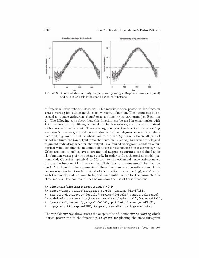
The main function of geofd is okfd (Table 1). This function allows to carry outpredictions by ordinary kriging for function-valued data by considering a Fourieror a B-splines basis as methods for smoothing the observed data set. This coversfrom the smoothing step and trace-variogram estimation to data prediction. Al-though the estimation of the trace-variogram can be obtained by directly usingthe function okfd, it is also possible to estimate it in a sequential way by usingthe functions l2.norm, trace.vari and fit.tracevariog, respectively (Table 1).Now we give an illustration in this sense. In this example the data set is smoothedby using a B-splines basis with 65 functions without penalization (Figure 3, leftpanel). The number of basis functions was chosen by cross-validation (Delicadoet al. 2010). We initially define the parameters for smoothing the data. We usehere the fda library. An overview of the smoothing functional data by means ofB-splines basis using the library fda library can be found in (Ramsay, Wickham,Graves & Hooker 2010). The following code illustrates how to run this processwith the maritime data set.

R> n<-dim(maritimes.data)[1]R> argvals<-seq(1,n, by=1)R> s<-35R> rangeval <- range(argvals)R> norder <- 4R> nbasis <- 65R> bspl.basis <- create.bspline.basis(rangeval, nbasis, norder)R> lambda <-0R> datafdPar <- fdPar(bspl.basis, Lfdobj=2, lambda)R> smfd <- smooth.basis(argvals,maritimes.data,datafdPar)R> datafd <- smfd$fdR> plot(datafd, lty=1, xlab="Day", ylab="Temperature (degrees C)")

The smoothed curves are shown in the left panel of Figure 3. Once wi havesmoothed the data, we can use the functions above for estimating the trace-variogram. First we have to calculate the L2 norm between the smoothed curvesusing the function l2.norm. The arguments for this function are the number s ofsites where curves are observed, datafd a functional data object representing asmoothed data set and M a symmetric matrix of order equal to the number of basisfunctions defined by the B-splines basis object, where each element is the innerproduct of two basis functions after applying the derivative or linear di�erentialoperator defined by Lfdobj (Ramsay et al. 2010).

R> M <- bsplinepen(bspl.basis,Lfdobj=0)R> L2norm <- l2.norm(s, datafd, M)

In the above commands the results are assigned to the variable L2norm. Thisone stores a matrix whose values correspond to the L2 norm between each pair



Figure 3: Smoothed data of daily temperature by using a B-splines basis (left panel)and a Fourier basis (right panel) with 65 functions.

of functional data into the data set. This matrix is then passed to the functiontrace.variog for estimating the trace-variogram function. The output can be re-turned as a trace-variogram “cloud" or as a binned trace-variogram (see Equation7). The following code shows how this function can be used in combination withfit.tracevariog for fitting a model to the trace-variogram function obtainedwith the maritime data set. The main arguments of the function trace.variogare coords the geographical coordinates in decimal degrees where data whererecorded, L2 norm a matrix whose values are the L2 norm between all pair ofsmoothed functions (an output from the function l2.norm), bin which is a logicalargument indicating whether the output is a binned variogram, maxdist a nu-merical value defining the maximum distance for calculating the trace-variogram.Other arguments such as uvec, breaks and nugget.tolerance are defined as inthe function variog of the package geoR. In order to fit a theoretical model (ex-ponential, Gaussian, spherical or Matern) to the estimated trace-variogram wecan use the function fit.tracevariog. This function makes use of the functionvariofit of geoR. The arguments of these functions are the estimations of thetrace-variogram function (an output of the function trace.variog), model a listwith the models that we want to fit, and some initial values for the parameters inthese models. The command lines below show the use of these functions.

R> dista=max(dist(maritimes.coords))*0.9R> tracev=trace.variog(maritimes.coords, L2norm, bin=FALSE,+ max.dist=dista,uvec="default",breaks="default",nugget.tolerance)R> models=fit.tracevariog(tracev, models=c("spherical","exponential",+ "gaussian","matern"),sigma2.0=2000, phi.0=4, fix.nugget=FALSE,+ nugget=0, fix.kappa=TRUE, kappa=1, max.dist.variogram=dista)

The variable tracev above stores the output of the function trace.variog whichis used posteriorly in the function plot.geofd for plotting the trace-variogram



Trac

e-va

riogr

am

Distance

Trace-variogram cloud

empirical trace variogramsphericalexponentialgaussianmatern

Distance

Trace-variogram bin

Trac

e-va

riogr

am

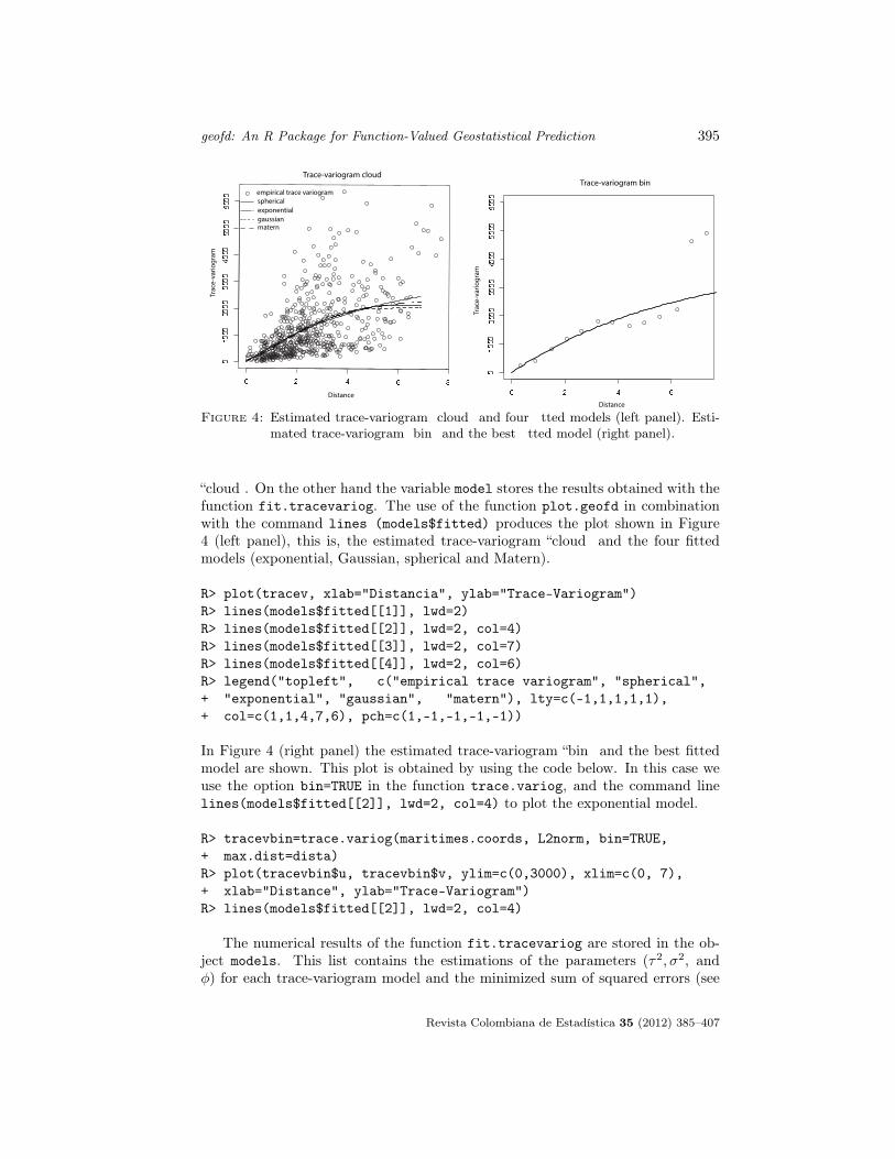
Figure 4: Estimated trace-variogram �cloud� and four �tted models (left panel). Esti-mated trace-variogram �bin� and the best �tted model (right panel).

“cloud�. On the other hand the variable model stores the results obtained with thefunction fit.tracevariog. The use of the function plot.geofd in combinationwith the command lines (models$fitted) produces the plot shown in Figure4 (left panel), this is, the estimated trace-variogram “cloud� and the four fittedmodels (exponential, Gaussian, spherical and Matern).

R> plot(tracev, xlab="Distancia", ylab="Trace-Variogram")R> lines(models$fitted[[1]], lwd=2)R> lines(models$fitted[[2]], lwd=2, col=4)R> lines(models$fitted[[3]], lwd=2, col=7)R> lines(models$fitted[[4]], lwd=2, col=6)R> legend("topleft", c("empirical trace variogram", "spherical",+ "exponential", "gaussian", "matern"), lty=c(-1,1,1,1,1),+ col=c(1,1,4,7,6), pch=c(1,-1,-1,-1,-1))

In Figure 4 (right panel) the estimated trace-variogram “bin� and the best fittedmodel are shown. This plot is obtained by using the code below. In this case weuse the option bin=TRUE in the function trace.variog, and the command linelines(models$fitted[[2]], lwd=2, col=4) to plot the exponential model.

R> tracevbin=trace.variog(maritimes.coords, L2norm, bin=TRUE,+ max.dist=dista)R> plot(tracevbin$u, tracevbin$v, ylim=c(0,3000), xlim=c(0, 7),+ xlab="Distance", ylab="Trace-Variogram")R> lines(models$fitted[[2]], lwd=2, col=4)

The numerical results of the function fit.tracevariog are stored in the ob-ject models. This list contains the estimations of the parameters (τ2, σ2, andφ) for each trace-variogram model and the minimized sum of squared errors (see



variofit from geoR). According to the results below we can observe that the bestmodel (least sum of squared errors) is the exponential model.

R>models

[[1]]variofit: model parameters estimated by OLS (ordinary least squares):covariance model is: sphericalfixed value for tausq = 0parameter estimates:

sigmasq phi3999.9950 12.0886Practical Range with cor=0.05 for asymptotic range: 12.08865variofit: minimised sum of squares = 529334304[[2]]variofit: model parameters estimated by OLS (ordinary least squares):covariance model is: exponentialfixed value for tausq = 0parameter estimates:

sigmasq phi4000.0003 6.2689Practical Range with cor=0.05 for asymptotic range: 18.77982variofit: minimised sum of squares = 524840646[[3]]variofit: model parameters estimated by OLS (ordinary least squares):covariance model is: gaussianfixed value for tausq = 0parameter estimates:

sigmasq phi2092.8256 2.2886Practical Range with cor=0.05 for asymptotic range: 3.961147variofit: minimised sum of squares = 541151209fitted[[4]]variofit: model parameters estimated by OLS (ordinary least squares):covariance model is: Matern with fixed kappa = 1fixed value for tausq = 0parameter estimates:

sigmasq phi2693.1643 1.9739Practical Range with cor=0.05 for asymptotic range: 7.892865variofit: minimised sum of squares = 529431348

Once fitted, the best trace-variogram model we can use the okfd function forperforming spatial prediction at an unvisited location. The arguments of thisfunction are new.coords an n × 2 matrix containing the coordinates of the newn prediction sites, coords an s × 2 matrix containing the coordinates of the ssites where functional data were recorded, data an m × s matrix with values



for the observed functions, smooth.type a string with the name of smoothingmethod to be used (B-splines or Fourier), nbasis a numeric value defining thenumber of basis functions used to smooth the discrete data set recorded at eachsite, argvals a vector containing argument values associated with the values tobe smoothed, lambda (optional) a penalization parameter for smoothing the ob-served functions, and cov.model a string with the name of the correlation function(see variofit from geoR). Other additional arguments are fix.nugget, nuggetvalue, fix.kappa, kappa (related to the parameters of the correlation model),and max.dist.variogram a numerical value defining the maximum distance con-sidered when fitting the variogram model. The code below allows to predict atemperature curve at the Moncton weather station (see Figure 1).

R> okfd.res<-okfd(new.coords=coord.cero, coords=maritimes.coords,+ cov.model="exponential", data=maritimes.data, nbasis=65,+ argvals=argvals, fix.nugget=TRUE)R> plot(okfd.res$datafd, lty=1,col=8, xlab="Day",+ ylab="Temperature (degrees C)",+ main="Prediction at Moncton")R> lines(okfd.res$argvals, okfd.res$krig.new.data, col=1, lwd=2,+ type="l", lty=1, main="Predictions", xlab="Day",+ ylab="Temperature (Degrees C)")R> lines(maritimes.avg, type="p", pch=20,cex=0.5, col=2, lwd=1)

A graphical comparison between real data (see maritimes.avg in Table 1) andthe predicted curve (Figure 5) allows to conclude that the method OKFD has agood performance with this data set.

Figure 5: Smoothed curves by using a B-splines basis with 65 functions (gray), realdata at Moncton weather station (red dots) and prediction at Moncton byordinary kriging for function-value spatial data.



3.2. Using a Fourier basis

Now we use the package geofd for carrying out spatial prediction of temperaturecurves at ten randomly selected locations in the Canadian Maritimes Provinces(Figure 2, right panel). We use a Fourier basis with 65 functions for smoothing thedata set (the same number of basis functions K as in Section 3.1) . In this examplewe show how the function okfd allows both smoothing the data and estimatingdirectly a trace-variogram model. Posteriorly the estimation is used for performingspatial predictions of temperature curves on the ten locations already mentioned.The R code is the following

R> argvals<-seq(1,n, by=1)R> col1<-sample((min(maritimes.coords[,1])*100):(max(maritimes.coords[,1]) + *100),10, replace=TRUE)/100R> col2<-sample((min(maritimes.coords[,2])*100):(max(maritimes.coords[,2]) + *100),10, replace=TRUE)/100R> new.coords <- cbind(col1,col2)

The variable argvals contains argument values associated with the values to besmoothed by using a Fourier basis. The variables col1, col2, and new.coordsare used for defining the prediction locations (Figure 2, right panel). The variableargvals and new.coords are used as arguments of the function okfd in the codebelow

R> okfd.res<-okfd(new.coords=new.coords, coords=maritimes.coords,+ data=maritimes.data, smooth.type="fourier", nbasis=65,+ argvals=argvals, kappa=0.7)

In this example the arguments smooth.type="fourier" and nbasis=65 in thefunction okfd allows us to smooth the data by using a Fourier basis with 65 func-tions (the number of basis functions was determined by cross-validation). In theexample in Section 3.1 we use directly cov.model="exponential" in the functionokfd because we chose this model previously by using the functions trace.variogand fit.tracevariog. If we do not specify a covariance model the function okfdestimates several models and selects the model with the least sum of squared errors.The parameter kappa=.7 indicates that in addition to the spherical, exponentialand Gaussian model, a Matern model with κ = .7 is also fitted.

A list with the objects stored in the variable okfd.res is obtained with thecommand line

R> names(okfd.res)

[1] "coords" "data"[3] "argvals" "nbasis"[5] "lambda" "new.coords"[7] "emp.trace.vari" "trace.vari"[9] "new.Eu.d" "functional.kriging.weights"



empirical trace variogramsphericalexponentialgaussianmatern

Trac

e-va

riogr

am

Trace-variogram cloud

Distance

Trac

e-va

riogr

am

Trace-variogram bin

Distance

Figure 6: Estimated trace-variogram �cloud� and four �tted models (left panel). Esti-mated trace-variogram �bin� and the best �tted model (right panel).

[11] "krig.new.data" "pred.var"[13] "trace.vari.array" "datafd"

We can use these objects for plotting the trace-variogram function, the esti-mated models and the predictions. A plot with the four fitted models and the bestmodel is shown in Figure 6. We obtain this figure by using the command lines

R> plot(okfd.res, ylim=c(0,6000))R> trace.variog.bin<-trace.variog(okfd.res$coords,+ okfd.res$emp.trace.vari$L2norm, bin=TRUE)R> plot(trace.variog.bin, ylim=c(0,6000), xlab="Distance",+ ylab="Trace-variogram", main="Trace-variogram Bin")R> lines(okfd.res$trace.vari, col=4, lwd=2)

Numerical results of the trace-variogram fitted models are obtained by using thecommand line

okfd.res$trace.vari.array

[[1]]variofit: model parameters estimated by OLS (ordinary least squares):covariance model is: sphericalparameter estimates:

tausq sigmasq phi178.4011 644834.9056 2328.6674

Practical Range with cor=0.05 for asymptotic range: 2328.667variofit: minimised sum of squares = 539799716[[2]]variofit: model parameters estimated by OLS (ordinary least squares):



covariance model is: exponentialparameter estimates:


Practical Range with cor=0.05 for asymptotic range: 69.34139variofit: minimised sum of squares = 539566326[[3]]variofit: model parameters estimated by OLS (ordinary least squares):covariance model is: gaussianparameter estimates:


Practical Range with cor=0.05 for asymptotic range: 5.818404variofit: minimised sum of squares = 552739397[[4]]variofit: model parameters estimated by OLS (ordinary least squares):covariance model is: matern with fixed kappa = 0.7parameter estimates:


Practical Range with cor=0.05 for asymptotic range: 20.31806variofit: minimised sum of squares = 541310787

The model with least sum of squared errors is again a exponential model (Figure6, right panel). Consequently the function okfd above uses this model for solvingthe system in Equation 5 and for carrying out the predictions. Numerical valuesof predictions and prediction variances can be checked by using the commands

R> okfd.res[11]R> okfd.res[12]

The predictions can be plotted by using the following command line

R>.geofd.viewer(okfd.res, argnames=c("Prediction","Day","Temperature"))

The function .geofd.viewer implements a Tcl/Tk interface (Grosjean 2010) forshowing OKFD prediction results. This viewer presents two frames, the left onepresents the spatial distribution of the prediction sites. The right one presentsthe selected prediction curve based on the point clicked by the user on the leftframe. In Figure 7 we show the result of using this function. In the left panel ascatterplot with the coordinates of the prediction locations are shown. The darkpoint in the left panel is the clicked point and, the curve in the right panel showsthe prediction at this site.

On the other hand if we want to plot all the predicted curves and analyze themsimultaneously we can use the following command line



Figure 7: An example of the function .geofd.viewer. Left panel: Scatterplot withthe coordinates of prediction locations. Right panel: Prediction on a clickedpoint (red point in left panel).

R> matplot(okfd.res$argvals, okfd.res$krig.new.data, col=1, lwd=1,type="l", + lty=1, main="Predictions", xlab="Day",ylab="Temperature (degrees C)")

We can observe that the predicted curves (Figure 8) are consistent with thebehavior of the original data set (Figure 1). This result indicates empirically thatthe OKFD method shows a good performance.

Predictions

Day

Tem

pera

ture

(deg

rees

C)

Figure 8: OKFD Predictions at ten randomly selected sites from Canadian MaritimesProvinces. Observed data were previously smoothed by using a Fourier basis.



−3 −2 −1 0 1 2

−3−2

−10

12

x

y

Site 1 Site 2 Site 3 Site 4 Site 5 Site 6






0 100 200 300

0.0

0.2

0.4

0.6

0.8

1.0

Time

Figure 9: Left panel: Grid of simulated locations. Right panel: B-splines basis used inthe simulation algorithm.

3.3. Using Simulated Data

In this section we discuss algorithms proposed in our package and evaluate theperformance of the methodologies proposed in Section 2 by means of a simulationstudy.

We fixed the thirty six sites shown in Figure 9, and simulated a discretized setof spatially correlated functional data according to the model

Xsi(t) =

15∑l=1

ailBl(t) + εi(t), i = 1, . . . , 36 (9)

with B(t) = (B1(t), . . . , B15(t)) a B-splines basis (see right panel Figure 9), ail,a realization of a Gaussian random field al ∼ N36(10,Σ), where Σ is a 36 × 36covariance matrix defined according to the exponential model C(h) = 2 exp(−h8 )with h = ‖si − sj‖, i, j = 1, . . . , 36, and ε(t) ∼ N36(0.09, 1) is a random error foreach fixed t, with t = 1, . . . , 365. The number of basis functions and the parametersfor simulating coefficients and errors were chosen empirically.

The R code for obtaining the simulated curves is the following

R> coordinates<-expand.grid(x= c(-3,-2, -1, 0, 1, 2),+ y=c(-3,-2,-1,0, 1, 2))R> mean.coef=rep(10,36)R> covariance.coef <- cov.spatial(distance, cov.model=model,+ cov.pars=c(2,8))R> normal.coef=mvrnorm(15,mean.coef,covariance.coef)R> mean.error<-rep(0, 36)R> covariance.error <-cov.spatial(distance, cov.model=model,+ cov.pars=c(0.09,0))R> normal.error<-mvrnorm(365,mean.error,covariance.error)R> argvals=seq(1, 365, len = 365)



R> nbasis=15R> lambda=0R> rangeval <- range(argvals)R> norder <- 4R> bspl.basis <- create.bspline.basis(rangeval, nbasis,+ norder)R> data.basis=eval.basis(argvals, bspl.basis, Lfdobj=0)R> func.data=t(normal.coef)%*%t(data.basis)R> simulated.data= func.data+ normal.error

A plot with the simulated data and smoothed curves (by using a B-splines basis)is obtained with the following code

R> datafdPar <- fdPar(bspl.basis, Lfdobj=2, lambda)R> smooth.datafd <- smooth.basis(argvals, simulated.data,+ datafdPar)R> simulated.smoothed=eval.fd(argvals, smooth.datafd$fd,+ fdobj=0)R> matplot(simulated.data, type="l", lty=1, xlab="Time",+ ylab="Simulated data")R> matplot(simulated.smoothed, lty=1, xlab="Time",+ ylab="Smoothed data", type="l")

The simulated data are shown in the left panel of Figure 10. These data weresmoothed by using a B-splines basis with 15 functions (right panel Figure 10).Once obtaining the smoothed curves we carry out a cross-validation predictionprocedure. Each data location in Figure 9 is removed from the dataset and asmoothed curve is predicted at this location using OKFD based on the remainingsmoothed functions.

Figure 10: Left panel: Simulated data. Right panel: Smoothed curves (by using aB-splines basis).

The R code for obtaining the cross-validation predictions is

R> predictions= matrix(0, nrow=365, ncol=36)



R> for (i in 1:36)R> {R> coord.cero=matrix(coordinates[i,], nrow=1,ncol=2)R> okfd.res<-okfd(new.coords=coord.cero,+ coords=coordinates[-i,], cov.model="exponential",+ data=simulated.data[,-i], smooth.type="bsplines",+ nbasis=15, argvals=argvals, fix.nugget=TRUE)R> predictions[,i]=okfd.res$krig.new.dataR> }

We can plot the cross-validation predictions and the cross-validation residuals byusing the following code

R> matplot(predictions, lty=1, xlab="Time",ylab="Predictions",+ main="Cross-validation predictions", type="l")R> cross.residuals=simulated.smoothed-predictionsR> matplot(cross.residuals, lty=1, xlab="Time",+ ylab="Residuals", main="Cross-validation residuals",+ type="l")

The cross-validation predictions (left panel Figure 11) shows that the predictionshave the same temporal behavior as the smoothed curves (right panel Figure 10).Note also that the prediction curves have less variance. This is not surprising,because kriging is itself a smoothing method.

Figure 11 (right panel) shows cross-validation residuals. The predictions areplausible in all sites because all the residual curves are varying around zero.

Figure 11: Left panel: Simulated data. Right panel: Smoothed curves (by using aB-splines basis).

The cross-validation results based on simulated data show a good performanceof the proposed predictor, and indicate from a descriptive point of view that it canbe adopted as a valid method for modeling spatially correlated functional data.



4. Conclusion

This paper introduces the R package geofd through an example. This packagecontains functions for modeling the trace-variogram function and for carrying outspatial prediction using the method of ordinary kriging for functional data. Theadvancements in this package would not be possible without several other impor-tant contributions to CRAN; these are re�ected as geofd's package dependencies.The fda package by (Ramsay et al. 2010) provides methods for smoothing data byusing basis functions. The geoR package (Ribeiro & Diggle 2001) provides func-tions to enable modeling the trace-variograma function. There remains scope forfurther extensions to geofd. We can consider other approaches for smoothing thedata. For example, the use of wavelets could be useful for smoothing data withrapid changes in behavior. We plan to continue adding methods to the package.Continuous time varying kriging (Giraldo et al. 2010) and methods based on multi-variable geostatistics (Giraldo 2009, Nerini et al. 2010) can be implemented in thepackage. However the use of these approaches could be restrictive when the num-ber of basis functions used for smoothing the data set is large. Computationallyefficient strategies are needed in this sense.

Acknowledgements

We would like to thank Andrés Pérez for his valuable contribution to upload thepackage geofd to CRAN. This work was partially supported by the Spanish Min-istry of Education and Science through grants MTM2010-14961 and MTM2009-13985-C02-01.[

Recibido: octubre de 2011 — Aceptado: agosto de 2012]

References

Baladandayuthapani, V., Mallick, B., Hong, M., Lupton, J., Turner, N. & Caroll,R. (2008), `Bayesian hierarchical spatially correlated functional data analysiswith application to colon carcinoginesis', Biometrics 64, 64�73.

Box, G. & Jenkins, G. (1976), Time Series Analysis., Holden Day, New York.

Cressie, N. (1993), Statistics for Spatial Data, John Wiley & Sons, New York.

Cuevas, A., Febrero, M. & Fraiman, R. (2004), `An ANOVA test for functionaldata.', Computational Statistics and Data Analysis 47, 111�122.

Delicado, P., Giraldo, R., Comas, C. & Mateu, J. (2010), `Statistics for spatialfunctional data: Some recent contributions', Environmetrics 21, 224�239.

Ferraty, F. & Vieu, P. (2006), Nonparametric Functional Data Analysis. Theoryand Practice, Springer, New York.



Giraldo, R. (2009), Geostatistical Analysis of Functional Data, PhD thesis, Uni-versitat Politècnica de Catalunya.

Giraldo, R., Delicado, P. & Mateu, J. (2010), `Continuous time-varying kriging forspatial prediction of functional data: An environmental application', Journalof Agricultural, Biological, and Environmental Statistics 15(1), 66�82.

Giraldo, R., Delicado, P. & Mateu, J. (2011), `Ordinary kriging for function-valuedspatial data', Environmental and Ecological Statistics 18(3), 411�426.

Goulard, M. & Voltz, M. (1993), Geostatistical interpolation of curves: A casestudy in soil science, in A. Soares, ed., `Geostatistics Tróia 92', Vol. 2, KluwerAcademc Press, pp. 805�816.

Grosjean, P. (2010), SciViews-R: A GUI API for R, UMONS, Mons, Belgium.*http://www.sciviews.org/SciViews-R

Malfait, N. & Ramsay, J. (2003), `The historical functional linear model', TheCanadian Journal of Statistics 31(2), 115�128.

MATLAB (2010), version 7.10.0 (R2010a), The MathWorks Inc., Natick, Mas-sachusetts.

Myers, D. (1982), `Matrix formulation of co-kriging', Mathematical Geology14(3), 249�257.

Nerini, D., Monestiez, P. & Manté, C. (2010), `Cokriging for spatial functionaldata', Journal of Multivariate Analysis 101(2), 409�418.

R Development Core Team (2011), R: A Language and Environment for StatisticalComputing, R Foundation for Statistical Computing, Vienna, Austria. ISBN3-900051-07-0.*http://www.R-project.org.

Ramsay, J., Hooker, G. & Graves, S. (2009), Functional Data Analysis with R andMATLAB, Springer, New York.

Ramsay, J. & Silverman, B. (2005), Functional Data Analysis. Second edition,Springer, New York.

Ramsay, J., Wickham, H., Graves, S. & Hooker, G. (2010), fda: Functional DataAnalysis. R package version 2.2.6.*http://cran.r-project.org/web/packages/fda

Ribeiro, P. & Diggle, P. (2001), `geoR: A package for geostatistical analysis', R-NEWS 1(2), 15�18.*http://cran.R-project.org/doc/Rnews

Staicu, A., Crainiceanu, C. & Carroll, R. (2010), `Fast methods for spatially cor-related multilevel functional data', Biostatistics 11(2), 177�194.



Ver Hoef, J. & Cressie, N. (1993), `Multivariable spatial prediction', MathematicalGeology 25(2), 219�240.

Wackernagel, H. (1995), Multivariate Geostatistics: An Introduction with Appli-cations, Springer-Verlag, Berlin.

Yamanishi, Y. & Tanaka, Y. (2003), `Geographically weighted functional multipleregression analysis: A numerical investigation', Journal of Japanese Societyof Computational Statistics 15, 307�317.


Redalyc.geofd: An R Package for Function-Valued ... · enlaestimacióndelafuncióntraza-variograma. Seilustraelpaqueteanal-izandodatosrealesysimulados. Palabras clave:...

Documents