© 2010 Pearson Prentice Hall. All rights reserved Chapter Estimating the Value of a Parameter Using Confidence Intervals 9

© 2010 Pearson Prentice Hall. All rights reserved Chapter Estimating the Value of a Parameter Using Confidence Intervals 9.
Dec 15, 2015
Welcome message from author
This document is posted to help you gain knowledge. Please leave a comment to let me know what you think about it! Share it to your friends and learn new things together.
Transcript

© 2010 Pearson Prentice Hall. All rights reserved
Chapter
Estimating the Value of a Parameter Using Confidence Intervals
9

© 2010 Pearson Prentice Hall. All rights reserved
Section
The Logic in Constructing Confidence Intervals for a Population Mean When the Population Standard Deviation Is Known
9.1

© 2010 Pearson Prentice Hall. All rights reserved 9-3
1. Compute a point estimate of the population mean2. Construct and interpret a confidence interval for the
population mean assuming that the population standard deviation is known
3. Understand the role of margin of error in constructing the confidence interval
4. Determine the sample size necessary for estimating the population mean within a specified margin of error
Objectives

© 2010 Pearson Prentice Hall. All rights reserved 9-4
Objective 1
• Compute a Point Estimate of the Population Mean

© 2010 Pearson Prentice Hall. All rights reserved 9-5
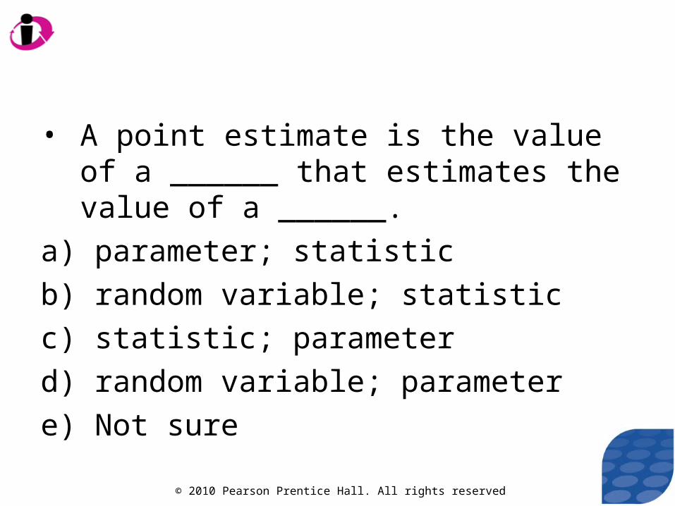
A point estimate is the value of a statistic that estimates the value of a parameter.
For example, the sample mean, , is a point estimate of the population mean .
x

© 2010 Pearson Prentice Hall. All rights reserved 9-6
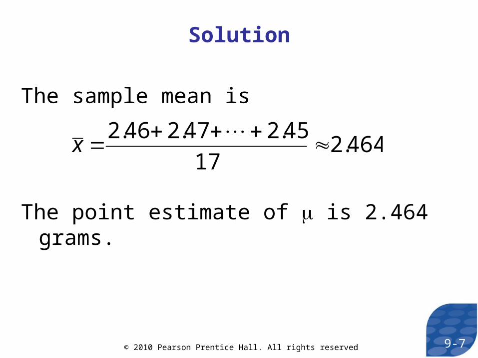
Pennies minted after 1982 are made from 97.5% zinc and 2.5% copper. The following data represent the weights (in grams) of 17 randomly selected pennies minted after 1982.
2.46 2.47 2.49 2.48 2.50 2.44 2.46 2.45 2.49
2.47 2.45 2.46 2.45 2.46 2.47 2.44 2.45
Treat the data as a simple random sample. Estimate the population mean weight of pennies minted after 1982.
Parallel Example 1: Computing a Point Estimate
© 2010 Pearson Prentice Hall. All rights reserved 9-7
The sample mean is
The point estimate of is 2.464 grams.
Solution
x 2.46 2.47 2.45
172.464
© 2010 Pearson Prentice Hall. All rights reserved
• A point estimate is the value of a ______ that estimates the value of a ______.
a) parameter; statistic
b) random variable; statistic
c) statistic; parameter
d) random variable; parameter
e) Not sure

© 2010 Pearson Prentice Hall. All rights reserved 9-9
Objective 2
• Construct and Interpret a Confidence Interval for the Population Mean

© 2010 Pearson Prentice Hall. All rights reserved 9-10
A confidence interval for an unknown parameter consists of an interval of numbers.
The level of confidence represents the expected proportion of intervals that will contain the parameter if a large number of different samples is obtained. The level of confidence is denoted
(1-)·100%.

© 2010 Pearson Prentice Hall. All rights reserved 9-11
For example, a 95% level of confidence
(=0.05) implies that if 100 different confidence intervals are constructed, each based on a different sample from the same population, we will expect 95 of the intervals to contain the parameter and 5 to not include the parameter.
© 2010 Pearson Prentice Hall. All rights reserved 9-12
• Confidence interval estimates for the population mean are of the form
Point estimate ± margin of error.
• The margin of error of a confidence interval estimate of a parameter is a measure of how accurate the point estimate is.

© 2010 Pearson Prentice Hall. All rights reserved 9-13
The margin of error depends on three factors:
1. Level of confidence: As the level of confidence increases, the margin of error also increases.
2. Sample size: As the size of the random sample increases, the margin of error decreases.
3. Standard deviation of the population: The more spread there is in the population, the wider our interval will be for a given level of confidence.

© 2010 Pearson Prentice Hall. All rights reserved 9-14
The shape of the distribution of all possible sample means will be normal, provided the population is normal or approximately normal, if the sample size is large (n≥30), with
• mean
• and standard deviation .
x
x n

© 2010 Pearson Prentice Hall. All rights reserved 9-15
Because is normally distributed, we know 95% of all sample means lie within 1.96 standard deviations of the population mean, , and 2.5% of the sample means lie in each tail.
x

© 2010 Pearson Prentice Hall. All rights reserved 9-16

© 2010 Pearson Prentice Hall. All rights reserved 9-17
95% of all sample means are in the interval
With a little algebraic manipulation, we can rewrite this inequality and obtain:
1.96n
x 1.96n

© 2010 Pearson Prentice Hall. All rights reserved 9-18
It is common to write the 95% confidence interval as
so that it is of the form
Point estimate ± margin of error.
.
x 1.96 x x 1.96 x
x 1.96 x

© 2010 Pearson Prentice Hall. All rights reserved 9-19
We will use Minitab to simulate obtaining 30 simple random samples of size n=8 from a population that is normally distributed with =50 and =10. Construct a 95% confidence interval for each sample. How many of the samples result in intervals that contain =50 ?
Parallel Example 2: Using Simulation to Demonstrate the Idea of a Confidence Interval

© 2010 Pearson Prentice Hall. All rights reserved 9-20
Sample Mean 95.0% CI C1 47.07 ( 40.14, 54.00)C2 49.33 ( 42.40, 56.26)C3 50.62 ( 43.69, 57.54)C4 47.91 ( 40.98, 54.84)C5 44.31 ( 37.38, 51.24)C6 51.50 ( 44.57, 58.43)C7 52.47 ( 45.54, 59.40)
C9 43.49 ( 36.56, 50.42)C10 55.45 ( 48.52, 62.38)C11 50.08 ( 43.15, 57.01)C12 56.37 ( 49.44, 63.30)C13 49.05 ( 42.12, 55.98)C14 47.34 ( 40.41, 54.27)C15 50.33 ( 43.40, 57.25)
C8 59.62 ( 52.69, 66.54)

© 2010 Pearson Prentice Hall. All rights reserved 9-21
SAMPLE MEAN 95% CIC16 44.81 ( 37.88, 51.74)C17 51.05 ( 44.12, 57.98)C18 43.91 ( 36.98, 50.84)C19 46.50 ( 39.57, 53.43)C20 49.79 ( 42.86, 56.72)C21 48.75 ( 41.82, 55.68)C22 51.27 ( 44.34, 58.20)C23 47.80 ( 40.87, 54.73)C24 56.60 ( 49.67, 63.52)C25 47.70 ( 40.77, 54.63)C26 51.58 ( 44.65, 58.51)C27 47.37 ( 40.44, 54.30)
C29 46.89 ( 39.96, 53.82)C30 51.92 ( 44.99, 58.85)
C28 61.42 ( 54.49, 68.35)
© 2010 Pearson Prentice Hall. All rights reserved 9-22
Note that 28 out of 30, or 93%, of the confidence intervals contain the population mean =50.
In general, for a 95% confidence interval, any sample mean that lies within 1.96 standard errors of the population mean will result in a confidence interval that contains .
Whether a confidence interval contains depends solely on the sample mean, .
x

© 2010 Pearson Prentice Hall. All rights reserved 9-23
Interpretation of a Confidence Interval
A (1-)·100% confidence interval indicates that, if we obtained many simple random samples of size n from the population whose mean, , is unknown, then approximately (1-)·100% of the intervals will contain .
For example, if we constructed a 99% confidence interval with a lower bound of 52 and an upper bound of 71, we would interpret the interval as follows: “We are 99% confident that the population mean, , is between 52 and 71.”

© 2010 Pearson Prentice Hall. All rights reserved 9-24
Constructing a (1- )·100% Confidence Interval for , Known
Suppose that a simple random sample of size n is taken from a population with unknown mean, , and known standard deviation . A (1-)·100% confidence interval for is given by
where is the critical Z-value.
Note: The sample size must be large (n≥30) or the population must be normally distributed.
z 2
Lower Upper Bound: Bound:
x z 2 n
x z 2 n

© 2010 Pearson Prentice Hall. All rights reserved 9-25
Construct a 99% confidence interval about the population mean weight (in grams) of pennies minted after 1982. Assume =0.02 grams.
2.46 2.47 2.49 2.48 2.50 2.44 2.46 2.45 2.49
2.47 2.45 2.46 2.45 2.46 2.47 2.44 2.45
Parallel Example 3: Constructing a Confidence Interval

© 2010 Pearson Prentice Hall. All rights reserved 9-26

© 2010 Pearson Prentice Hall. All rights reserved 9-27
Weight (in grams) of Pennies

© 2010 Pearson Prentice Hall. All rights reserved 9-28
• • Lower bound:
= 2.464-2.575
= 2.464-0.012 = 2.452
• Upper bound:
= 2.464+2.575
= 2.464+0.012 = 2.476We are 99% confident that the mean weight of penniesminted after 1982 is between 2.452 and 2.476 grams.
z 2 2.575
x z 2 n
0.0217
x z 2 n
0.0217

© 2010 Pearson Prentice Hall. All rights reserved
• A confidence interval for a parameter is
a) A point estimate plus a margin of error.
b) An interval of probabilities concerning a parameter.
c) An interval of numbers combined with the likelihood the interval contains the unknown parameter.
d) A statement of believability of a statistical result.
e) Not sure

© 2010 Pearson Prentice Hall. All rights reserved
Chapter 9 – Section 1
• True or False: A confidence interval with a 95% level of confidence means that the parameter will be in the interval approximately 95 times out of 100 samples.

© 2010 Pearson Prentice Hall. All rights reserved
• If the sample mean is 9, which of these could reasonably be a confidence interval for the population mean?a) 92
b) Lower bound: 3, Upper bound: 6
c) Lower bound: 7, Upper bound: 11
d) Lower bound: 0, Upper bound 25
e) Not sure

© 2010 Pearson Prentice Hall. All rights reserved
• Compute the critical value zα/2 that corresponds to a 95% level of confidence.

© 2010 Pearson Prentice Hall. All rights reserved 9-33
Objective 3
• Understand the Role of the Margin of Error in Constructing a Confidence Interval

© 2010 Pearson Prentice Hall. All rights reserved 9-34
The margin of error, E, in a (1-)·100% confidence interval in which is known is given by
where n is the sample size.
Note: We require that the population from which the sample was drawn be normally distributed or the samples size n be greater than or equal to 30.
E z 2 n

© 2010 Pearson Prentice Hall. All rights reserved 9-35
Parallel Example 5: Role of the Level of Confidence in the Margin of Error
Construct a 90% confidence interval for the mean weight of pennies minted after 1982. Comment on the effect that decreasing the level of confidence has on the margin of error.

© 2010 Pearson Prentice Hall. All rights reserved 9-36
• • Lower bound:
= 2.464-1.645
= 2.464-0.008 = 2.456
• Upper bound:
= 2.464+1.645
= 2.464+0.008 = 2.472We are 90% confident that the mean weight of penniesminted after 1982 is between 2.456 and 2.472 grams.
z 2 1.645
x z 2 n
0.0217
x z 2 n
0.0217

© 2010 Pearson Prentice Hall. All rights reserved 9-37
Notice that the margin of error decreased from 0.012 to 0.008 when the level of confidence decreased from 99% to 90%. The interval is therefore wider for the higher level of confidence.
Confidence Level
Margin ofError
Confidence Interval
90% 0.008 (2.456, 2.472)
99% 0.012 (2.452, 2.476)

© 2010 Pearson Prentice Hall. All rights reserved 9-38
Parallel Example 6: Role of Sample Size in the Margin of Error
Suppose that we obtained a simple random sample of pennies minted after 1982. Construct a 99% confidence interval with n=35. Assume the larger sample size results in the same sample mean, 2.464. The standard deviation is still =0.02. Comment on the effect increasing sample size has on the width of the interval.
© 2010 Pearson Prentice Hall. All rights reserved 9-39
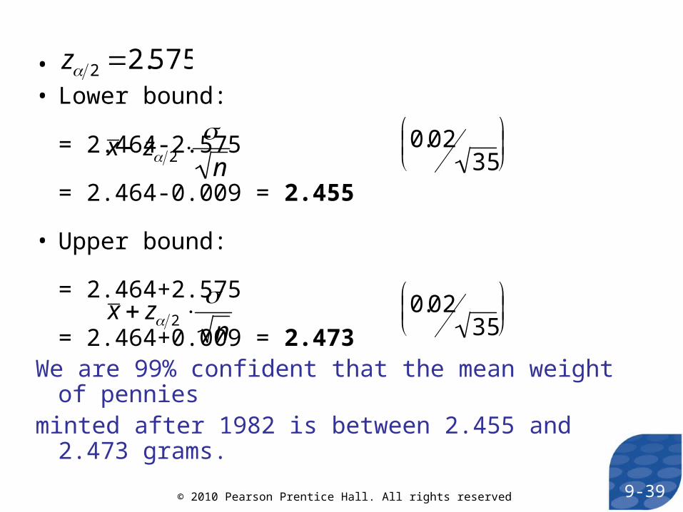
• • Lower bound:
= 2.464-2.575
= 2.464-0.009 = 2.455
• Upper bound:
= 2.464+2.575
= 2.464+0.009 = 2.473We are 99% confident that the mean weight of penniesminted after 1982 is between 2.455 and 2.473 grams.
z 2 2.575
x z 2 n
0.0235
x z 2 n
0.0235

© 2010 Pearson Prentice Hall. All rights reserved 9-40
Notice that the margin of error decreased from 0.012 to 0.009 when the sample size increased from 17 to 35. The interval is therefore narrower for the larger sample size.
Sample
Size
Margin ofError
Confidence Interval
17 0.012 (2.452, 2.476)
35 0.009 (2.455, 2.473)
© 2010 Pearson Prentice Hall. All rights reserved
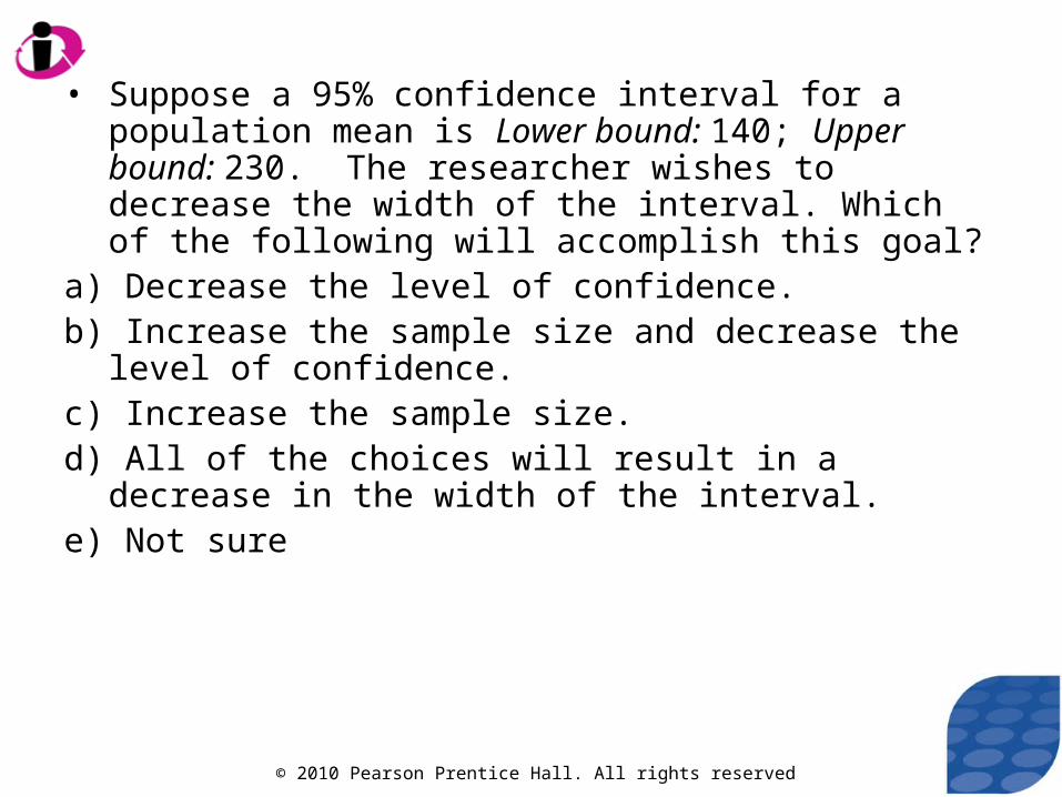
• Suppose a 95% confidence interval for a population mean is Lower bound: 140; Upper bound: 230. The researcher wishes to decrease the width of the interval. Which of the following will accomplish this goal?
a) Decrease the level of confidence.b) Increase the sample size and decrease the level of
confidence.c) Increase the sample size.d) All of the choices will result in a decrease in the width
of the interval.e) Not sure

© 2010 Pearson Prentice Hall. All rights reserved
• Suppose a 90% confidence interval for the population mean is Lower bound: 130; Upper bound: 300. Based on this interval, do you believe the mean of the population is equal to 320?
a) No, and I am 90% sure of it.
b) No, and I am 100% sure of it.
c) Yes, and I am 100% sure of it.
d) Yes, and I am 90% sure of it.
e) Not sure

© 2010 Pearson Prentice Hall. All rights reserved
• True or False: As the level of confidence increases, the margin of error decreases.

© 2010 Pearson Prentice Hall. All rights reserved 9-44
Objective 4
• Determine the Sample Size Necessary for Estimating the Population Mean within a Specified Margin of Error

© 2010 Pearson Prentice Hall. All rights reserved 9-45
Determining the Sample Size n
The sample size required to estimate the population mean, , with a level of confidence (1-)·100% with a specified margin of error, E, is given by
where n is rounded up to the nearest whole number.
n z
2
E
2

© 2010 Pearson Prentice Hall. All rights reserved 9-46
Back to the pennies. How large a sample would be required to estimate the mean weight of a penny manufactured after 1982 within 0.005 grams with 99% confidence? Assume =0.02.
Parallel Example 7: Determining the Sample Size

© 2010 Pearson Prentice Hall. All rights reserved 9-47
• =0.02
• E=0.005
•
Rounding up, we find n=107.
z 2 z0.005 2.575
n z
2
E
2
2.575(0.02)
0.005
2
106.09

© 2010 Pearson Prentice Hall. All rights reserved
Section
Confidence Intervals about a Population Mean When the Population Standard Deviation is Unknown
9.2

© 2010 Pearson Prentice Hall. All rights reserved 9-49
Objectives
1. Know the properties of Student’s
t-distribution
2. Determine t-values
3. Construct and interpret a confidence interval for a population mean

© 2010 Pearson Prentice Hall. All rights reserved 9-50
Objective 1
• Know the Properties of Student’s
t-Distribution

© 2010 Pearson Prentice Hall. All rights reserved 9-51
Suppose that a simple random sample of size n is taken from a population. If the population from which the sample is drawn follows a normal distribution, the distribution of
follows Student’s t-distribution with n-1 degrees of freedom where is the sample mean and s is the sample standard deviation.
Student’s t-Distribution
t x
s
n
x
© 2010 Pearson Prentice Hall. All rights reserved 9-52
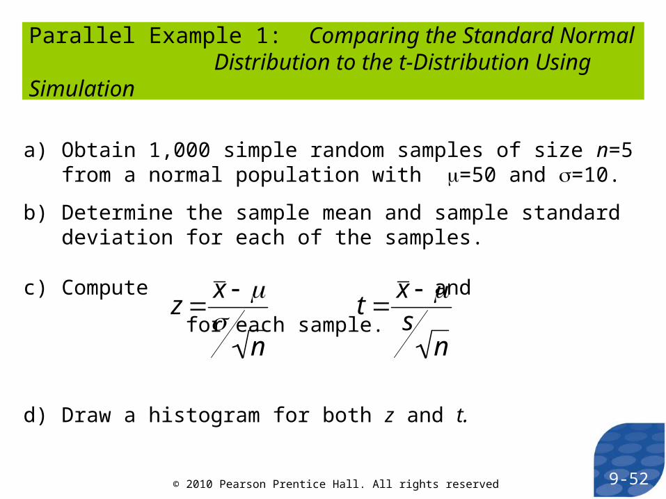
a) Obtain 1,000 simple random samples of size n=5 from a normal population with =50 and =10.
b) Determine the sample mean and sample standard deviation for each of the samples.
c) Compute and for each sample.
d) Draw a histogram for both z and t.
Parallel Example 1: Comparing the Standard Normal Distribution to the t-Distribution Using Simulation
z x
n
t x s
n

© 2010 Pearson Prentice Hall. All rights reserved 9-53
Histogram for z

© 2010 Pearson Prentice Hall. All rights reserved 9-54
Histogram for t

© 2010 Pearson Prentice Hall. All rights reserved 9-55
CONCLUSIONS:
• The histogram for z is symmetric and bell-shaped with the center of the distribution at 0 and virtually all the rectangles between -3 and 3. In other words, z follows a standard normal distribution.
• The histogram for t is also symmetric and bell-shaped with the center of the distribution at 0, but the distribution of t has longer tails (i.e., t is more dispersed), so it is unlikely that t follows a standard normal distribution. The additional spread in the distribution of t can be attributed to the fact that we use s to find t instead of . Because the sample standard deviation is itself a random variable (rather than a constant such as ), we have more dispersion in the distribution of t.

© 2010 Pearson Prentice Hall. All rights reserved 9-56
1. The t-distribution is different for different degrees of freedom.
2. The t-distribution is centered at 0 and is symmetric about 0.
3. The area under the curve is 1. The area under the curve to the right of 0 equals the area under the curve to the left of 0 equals 1/2.
4. As t increases without bound, the graph approaches, but never equals, zero. As t decreases without bound, the graph approaches, but never equals, zero.
Properties of the t-Distribution

© 2010 Pearson Prentice Hall. All rights reserved 9-57
5. The area in the tails of the t-distribution is a little greater than the area in the tails of the standard normal distribution, because we are using s as an estimate of , thereby introducing further variability into the t- statistic.
6. As the sample size n increases, the density curve of t gets closer to the standard normal density curve. This result occurs because, as the sample size n increases, the values of s get closer to the values of , by the Law of Large Numbers.
Properties of the t-Distribution

© 2010 Pearson Prentice Hall. All rights reserved 9-58

© 2010 Pearson Prentice Hall. All rights reserved 9-59
Objective 2
• Determine t-Values

© 2010 Pearson Prentice Hall. All rights reserved 9-60
© 2010 Pearson Prentice Hall. All rights reserved 9-61
Parallel Example 2: Finding t-values
Find the t-value such that the area under the t-distribution to the right of the t-value is 0.2 assuming 10 degrees of freedom. That is, find t0.20 with 10 degrees of freedom.

© 2010 Pearson Prentice Hall. All rights reserved 9-62
The figure to the left shows the graph of the t-distribution with 10 degrees of freedom.
Solution
The unknown value of t is labeled, and the area under the curve to the right of t is shaded. The value of t0.20 with 10 degrees of freedom is 0.8791.

© 2010 Pearson Prentice Hall. All rights reserved
• Find the t-value such that the area under the t-distribution with 10 degrees of freedom to the right of the t-value is 0.05.

© 2010 Pearson Prentice Hall. All rights reserved 9-64
Objective 3
• Construct and Interpret a Confidence Interval for a Population Mean

© 2010 Pearson Prentice Hall. All rights reserved 9-65
Constructing a (1-)100% Confidence Interval for , Unknown
Suppose that a simple random sample of size n is taken from a population with unknown mean and unknown standard deviation . A (1-)100% confidence interval for is given by
Lower Upperbound: bound:
Note: The interval is exact when the population is normally distributed. It is approximately correct for nonnormal populations, provided that n is large enough.
x t2
s
n
x t2
s
n

© 2010 Pearson Prentice Hall. All rights reserved 9-66
Parallel Example 3: Constructing a Confidence Interval about a Population Mean
The pasteurization process reduces the amount of bacteria found in dairy products, such as milk. The following data represent the counts of bacteria in pasteurized milk (in CFU/mL) for a random sample of 12 pasteurized glasses of milk. Data courtesy of Dr. Michael Lee, Professor, Joliet Junior College.
Construct a 95% confidence interval for the bacteria count.

© 2010 Pearson Prentice Hall. All rights reserved 9-67
NOTE: Each observation is in tens of thousand. So, 9.06 represents 9.06 x 10⁴.

© 2010 Pearson Prentice Hall. All rights reserved 9-68
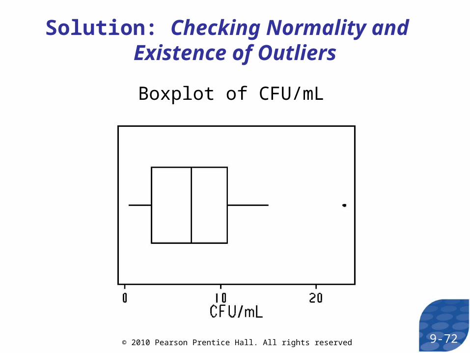
Solution: Checking Normality and Existence of Outliers

© 2010 Pearson Prentice Hall. All rights reserved 9-69
Boxplot of CFU/mL
Solution: Checking Normality and Existence of Outliers

© 2010 Pearson Prentice Hall. All rights reserved 9-70
x 6.41 and s 4.55
Lowerbound:
Upperbound:
The 95% confidence interval for the mean bacteria count in pasteurized milk is (3.52, 9.30).
•
•
0.05, n 12, so t 0.05
2
2.201
6.41 2.2014.55
123.52
6.41 2.2014.55
129.30

© 2010 Pearson Prentice Hall. All rights reserved 9-71
Parallel Example 5: The Effect of Outliers
Suppose a student miscalculated the amount of bacteria and recorded a result of 2.3 x 10⁵. We would include this value in the data set as 23.0.
What effect does this additional observation have on the 95% confidence interval?
© 2010 Pearson Prentice Hall. All rights reserved 9-72
Boxplot of CFU/mL
Solution: Checking Normality and Existence of Outliers

© 2010 Pearson Prentice Hall. All rights reserved 9-73
x 7.69 and s 6.34
Lowerbound:
Upperbound:
The 95% confidence interval for the mean bacteria count in pasteurized milk, including the outlieris (3.86, 11.52).
•
•
0.05, n 13, so t0.05
2
2.179
Solution
7.69 2.1796.34
133.86
7.69 2.1796.34
1311.52

© 2010 Pearson Prentice Hall. All rights reserved 9-74
CONCLUSIONS:
• With the outlier, the sample mean is larger because the sample mean is not resistant
• With the outlier, the sample standard deviation is larger because the sample standard deviation is not resistant
• Without the outlier, the width of the interval decreased from 7.66 to 5.78.
s 95% CI
Without
Outlier
6.41 4.55 (3.52, 9.30)
With
Outlier
7.69 6.34 (3.86, 11.52)
x

© 2010 Pearson Prentice Hall. All rights reserved
• A researcher collected 15 data points that seem to be reasonably bell shaped. Which distribution should the researcher use to calculate confidence intervals?a) A t-distribution with 14 degrees of freedom
b) A t-distribution with 15 degrees of freedom
c) A general normal distribution
d) A nonparametric method
e) Not sure
© 2010 Pearson Prentice Hall. All rights reserved
• Suppose a researcher wants to estimate the mean number of minutes students spend on their cell phones each week. He randomly selects 20 students and asks them to report the number of minutes they used their cell phone for the week. Based on the sample of 20 students, the mean number of minutes was 48.3 and the standard deviation was 10.8. What is the lower bound on a 95% confidence interval for the number of minutes spent using a cell phone for the week?

© 2010 Pearson Prentice Hall. All rights reserved
Section
Confidence Intervals for a Population Proportion
9.3

© 2010 Pearson Prentice Hall. All rights reserved 9-78
Objectives
1. Obtain a point estimate for the population proportion
2. Construct and interpret a confidence interval for the population proportion
3. Determine the sample size necessary for estimating a population proportion within a specified margin of error

© 2010 Pearson Prentice Hall. All rights reserved 9-79
Objective 1
• Obtain a point estimate for the population proportion

© 2010 Pearson Prentice Hall. All rights reserved 9-80
A point estimate is an unbiased estimator of
the parameter. The point estimate for the
population proportion is where x is
the number of individuals in the sample
with the specified characteristic and n is
the sample size.
ˆ p x
n

© 2010 Pearson Prentice Hall. All rights reserved 9-81
In July of 2008, a Quinnipiac University Poll asked 1783 registered voters nationwide whether they favored or opposed the death penalty for persons convicted of murder. 1123 were in favor.
Obtain a point estimate for the proportion of registered voters nationwide who are in favor of the death penalty for persons convicted of murder.
Parallel Example 1: Calculating a Point Estimate for the Population Proportion

© 2010 Pearson Prentice Hall. All rights reserved 9-82
Obtain a point estimate for the proportion of registered voters nationwide who are in favor of the death penalty for persons convicted of murder.
Solution
ˆ p 1123
17830.63

© 2010 Pearson Prentice Hall. All rights reserved
• Suppose a survey is conducted in which 500 eighteen year old freshman college students are asked whether they called their parents in the past week. Of the 500 surveyed, 340 indicated that they called their parents in the past week. Find a point estimate for the proportion of eighteen year old freshman college students that called their parents in the past week.

© 2010 Pearson Prentice Hall. All rights reserved 9-84
Objective 2
• Construct and Interpret a Confidence Interval for the Population Proportion
© 2010 Pearson Prentice Hall. All rights reserved 9-85
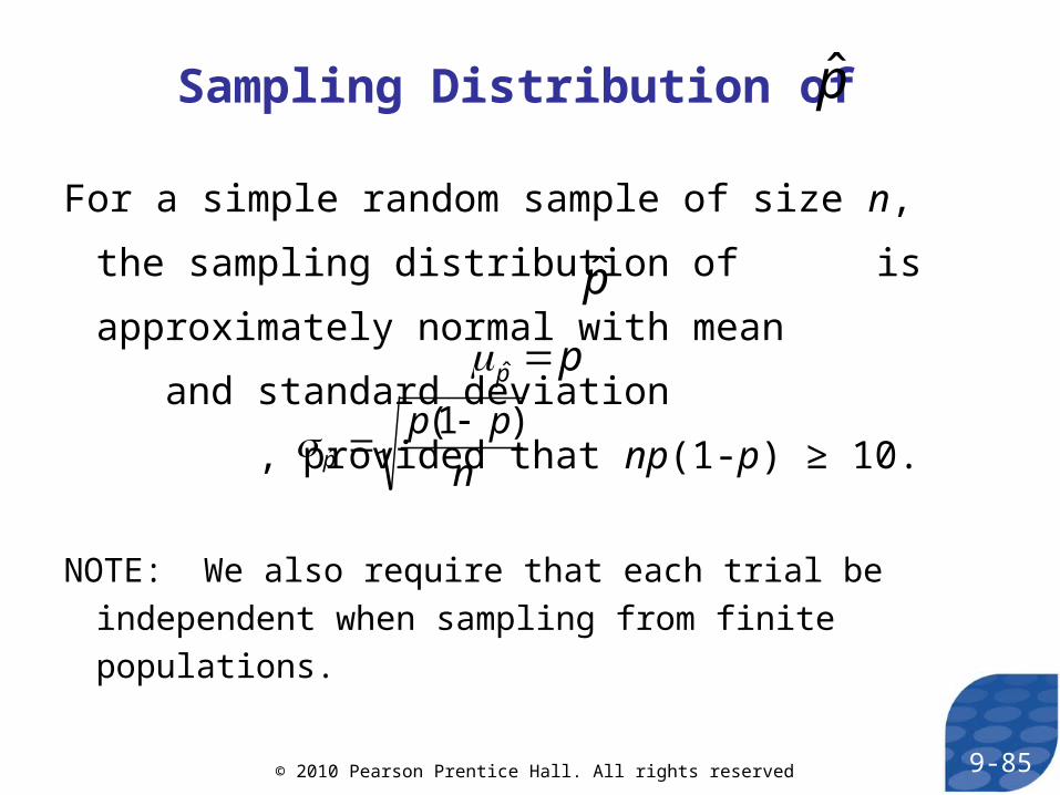
For a simple random sample of size n, the sampling
distribution of is approximately normal with
mean and standard deviation
, provided that np(1-p) ≥ 10.
NOTE: We also require that each trial be independent
when sampling from finite populations.
Sampling Distribution of
ˆ p
ˆ p
ˆ p p
ˆ p p(1 p)
n

© 2010 Pearson Prentice Hall. All rights reserved 9-86
Suppose that a simple random sample of size n is taken from a population. A (1-)·100% confidence interval for p is given by the following quantities
Lower bound:
Upper bound:
Note: It must be the case that and
n ≤ 0.05N to construct this interval.
Constructing a (1-)·100% Confidence Interval for a Population Proportion
ˆ p z 2 ˆ p (1 ˆ p )
n
ˆ p z 2 ˆ p (1 ˆ p )
n
nˆ p (1 ˆ p ) 10

© 2010 Pearson Prentice Hall. All rights reserved 9-87
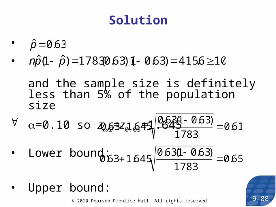
In July of 2008, a Quinnipiac University Poll asked 1783 registered voters nationwide whether they favored or opposed the death penalty for persons convicted of murder. 1123 were in favor.
Obtain a 90% confidence interval for the proportion of registered voters nationwide who are in favor of the death penalty for persons convicted of murder.
Parallel Example 2: Constructing a Confidence Interval for a Population Proportion
© 2010 Pearson Prentice Hall. All rights reserved 9-88
•
• and the sample size is definitely less than 5% of the population size
=0.10 so z/2=z0.05=1.645
• Lower bound:
• Upper bound:
ˆ p 0.63
nˆ p (1 ˆ p ) 1783(0.63)(1 0.63) 415.6 10
Solution
0.63 1.6450.63(1 0.63)
17830.61
0.631.6450.63(1 0.63)
17830.65

© 2010 Pearson Prentice Hall. All rights reserved 9-89
Solution
We are 90% confident that the proportion of registered voters who are in favor of the death penalty for those convicted of murder is between 0.61and 0.65.

© 2010 Pearson Prentice Hall. All rights reserved
• Suppose a survey is conducted in which 500 eighteen year old freshman college students are asked whether they called their parents in the past week. Of the 500 surveyed, 340 indicated that they called their parents in the past week. What is the margin of error (rounded to two decimal places) if we wanted to obtain a 95% confidence interval for the proportion of eighteen year old freshman college students that called their parents in the past week.

© 2010 Pearson Prentice Hall. All rights reserved 9-91
Objective 3
• Determine the Sample Size Necessary for Estimating a Population Proportion within a Specified Margin of Error

© 2010 Pearson Prentice Hall. All rights reserved 9-92
Sample size needed for a specified margin of error, E, and level of confidence (1-):
Problem: The formula uses which depends on n, the quantity we are trying to determine!
ˆ p
n ˆ p (1 ˆ p )z 2
E
2

© 2010 Pearson Prentice Hall. All rights reserved 9-93
Two possible solutions:
1. Use an estimate of p based on a pilot study or an earlier study.
2. Let =0.5 which gives the largest possible value of n for a given
level of confidence and a given
margin of error.
ˆ p

© 2010 Pearson Prentice Hall. All rights reserved 9-94
The sample size required to obtain a (1-)·100% confidence interval for p with a margin of error E is given by
(rounded up to the next integer), where is a prior estimate of p. If a prior estimate of p is unavailable, the sample size required is
ˆ p
n ˆ p (1 ˆ p )z 2
E
2
n 0.25z 2
E
2

© 2010 Pearson Prentice Hall. All rights reserved 9-95
A sociologist wanted to determine the percentage of residents of America that only speak English at home. What size sample should be obtained if she wishes her estimate to be within 3 percentage points with 90% confidence assuming she uses the 2000 estimate obtained from the Census 2000 Supplementary Survey of 82.4%?
Parallel Example 4: Determining Sample Size

© 2010 Pearson Prentice Hall. All rights reserved 9-96
• E=0.03
•
•
•
We round this value up to 437. The sociologist must
survey 437 randomly selected American residents.
z 2 z0.05 1.645
ˆ p 0.824
n 0.824(1 0.824)1.645
0.03
2
436.04
Solution

© 2010 Pearson Prentice Hall. All rights reserved
Section
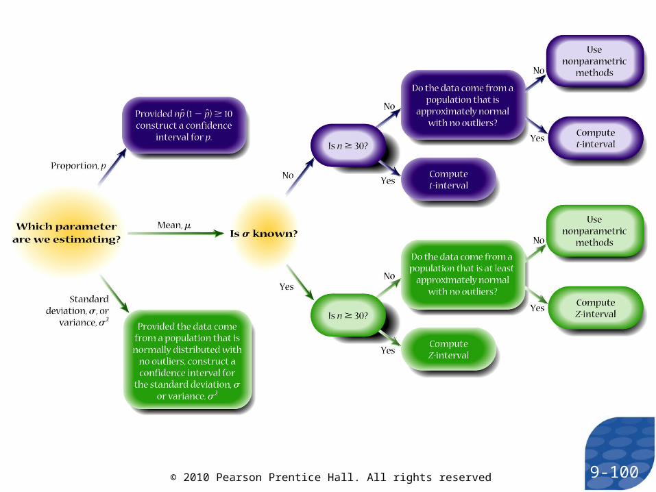
Putting It Together: Which Procedure Do I Use?
9.5

© 2010 Pearson Prentice Hall. All rights reserved 9-98
Objective
1. Determine the appropriate confidence interval to construct

© 2010 Pearson Prentice Hall. All rights reserved 9-99
Objective 1
• Determine the Appropriate Confidence Interval to Construct
© 2010 Pearson Prentice Hall. All rights reserved 9-100
Related Documents