© 2009 Pearson Education, Inc publishing as Prentice Hall 16-1 Chapter 16 Data Analysis: Frequency Distribution, Hypothesis Testing, and Cross-Tabulation.

© 2009 Pearson Education, Inc publishing as Prentice Hall 16-1

Chapter 16Chapter 16Data Analysis:

Frequency Distribution, Hypothesis Testing, and

Cross-Tabulation


Figure 16.1 Relationship of Frequency Distribution, Hypothesis Testing, and Cross-Tabulation to the Previous Chapters and the

Marketing Research Process

Focus of This Chapter

Relationship toPrevious Chapters

Relationship to MarketingResearch Process

• Frequency

• General Procedure for Hypothesis Testing

• Cross Tabulation

• Research Questions and Hypothesis (Chapter 2)

• Data Analysis Strategy (Chapter 15)

Problem Definition

Approach to Problem

Field Work

Data Preparation and Analysis

Report Preparationand Presentation

Research Design

© 2009 Pearson Education, Inc publishing as Prentice Hall 16-3Technology

Application to Contemporary Issues (Figs 16.12 – 16.14)EthicsInternational

Be

a D

M!

B

e an

MR

!

Exp

erie

nti

al L

earn

ing

Opening Vignette

Wh

at Wo

uld

Yo

u D

o?

Fig 16.10

Figure 16.2 Frequency Distribution, Hypothesis Testing, andCross Tabulation: An Overview

Frequency Distribution

Statistics Associated With Frequency Distribution

Introduction to Hypothesis Testing

Cross Tabulation

Statistics Associated With Cross Tabulation

Cross Tabulation in Practice

Tables 16.1-16.2 Fig 16.3-16.4

Tables 16.3-16.5

Fig 16.5

Fig 16.6-16.9

Fig 16.10

Fig 16.11


Frequency Distribution

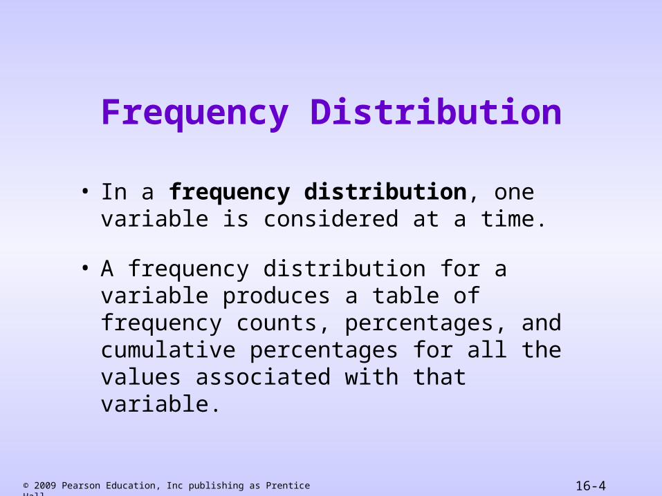
• In a frequency distribution, one variable is considered at a time.

• A frequency distribution for a variable produces a table of frequency counts, percentages, and cumulative percentages for all the values associated with that variable.


Calculate the Frequency for Each Value of the Variable

Calculate the Percentage and Cumulative Percentage

for Each Value, Adjusting for Any Missing Values

Plot the Frequency Histogram

Calculate the Descriptive Statistics, Measures of Location, and Variability

Figure 16.3 Conducting Frequency Analysis



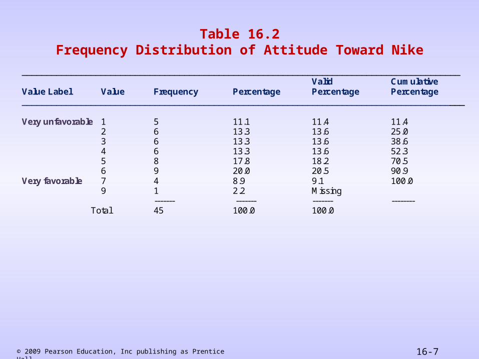
_________________________________________________________________________________________ Valid Cumulative Value Label Value Frequency Percentage Percentage Percentage __________________________________________________________________________________________ Very unfavorable 1 5 11.1 11.4 11.4 2 6 13.3 13.6 25.0 3 6 13.3 13.6 38.6 4 6 13.3 13.6 52.3 5 8 17.8 18.2 70.5 6 9 20.0 20.5 90.9 Very favorable 7 4 8.9 9.1 100.0 9 1 2.2 Missing ------- ------- ------- -------- Total 45 100.0 100.0

Table 16.2Frequency Distribution of Attitude Toward Nike


Table 16.2 (Cont.)Frequency Distribution of Attitude Toward Nike

Value Label Value Frequency Percentage Valid Percentage

Cumulative Percentage

Very unfavorable

Very favorable

1

2

3

4

5

6

7

9

5

6

6

6

8

9

4

1

11.1

13.3

13.3

13.3

17.8

20.0

8.9

2.2

11.4

13.6

13.6

13.6

18.2

20.5

9.1

Missing

11.4

25.0

38.6

52.3

70.5

90.9

100.0

Total 45 100.0 100.0 100.0


Figure 16.4 Frequency Histogram

0

1

2

3

4

5

6

7

8

9

Fre

qu

en

cy

1 2 3 4 5 6 7

Attitude Toward Nike


Statistics Associated with Frequency DistributionMeasures of Location

• The mean, or average value, is the most commonly used measure of central tendency.

Where, Xi = Observed values of the variable X n = Number of observations (sample size)

• The mode is the value that occurs most frequently. It represents the highest peak of the distribution.

The mean, X is given by

X = X i/n

i=1

n


• The median of a sample is the middle value when the data are arranged in ascending or descending order. If the number of data points is even, the median is usually estimated as the midpoint between the two middle values – by adding the two middle values and dividing their sum by 2. The median is the 50th percentile.

Statistics Associated with Frequency DistributionMeasures of Location


• The range measures the spread of the data. It is simply the difference between the largest and smallest values in the sample. Range = -

Statistics Associated with Frequency DistributionMeasures of Variability

larX gest smallestX


• The variance is the mean squared deviation from the mean. The variance can never be negative.

• The standard deviation is the square root of the variance.

==

( - )2

n- 1i 1

n

Statistics Associated with Frequency DistributionMeasures of Variability

xS iX X


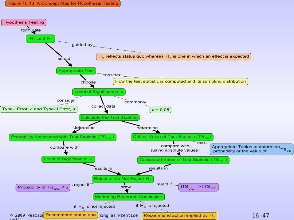
Figure 16.6 A General Procedure for Hypothesis Testing

Step 1

Step 2

Step 3

Step 4

Step 5

Step 6

Step 7

Step 8

Formulate H0 and H1

Select Appropriate Test

Choose Level of Significance, α

Collect Data and Calculate Test Statistic

Determine ProbabilityAssociated with Test

Statistic (TSCAL)

Determine CriticalValue of Test Statistic

TSCR

Compare with Level of Significance, α

Determine if TSCAL fallsinto (Non) Rejection Region

Reject or Do Not Reject H0

Draw Marketing Research Conclusion

a) b)

a) b)


A General Procedure for Hypothesis TestingStep 1: Formulate the Hypothesis

• A null hypothesis is a statement of the status quo, one of no difference or no effect. If the null hypothesis is not rejected, no changes will be made.

• An alternative hypothesis is one in which some difference or effect is expected. Accepting the alternative hypothesis will lead to changes in opinions or actions.

• The null hypothesis refers to a specified value of the population parameter (e.g., ), not a sample statistic (e.g., ).

, , X


• A null hypothesis may be rejected, but it can never be accepted based on a single test. In classical hypothesis testing, there is no way to determine whether the null hypothesis is true.

• In marketing research, the null hypothesis is formulated in such a way that its rejection leads to the acceptance of the desired conclusion. The alternative hypothesis represents the conclusion for which evidence is sought.

H0: 0.40

H1: > 0.40

A General Procedure for Hypothesis TestingStep 1: Formulate the Hypothesis (Cont.)


• The test of the null hypothesis is a one-tailed test, because the alternative hypothesis is expressed directionally. If that is not the case, then a two-tailed test would be required, and the hypotheses would be expressed as:

H0: = 0.40

H1: 0.40

A General Procedure for Hypothesis TestingStep 1: Formulate the Hypothesis (Cont.)


• The test statistic measures how close the sample has come to the null hypothesis and follows a well-known distribution, such as the normal, t, or chi-square.

• In our example, the z statistic, which follows the standard normal distribution, would be appropriate.

A General Procedure for Hypothesis TestingStep 2: Select an Appropriate Test

z = p - p

where

p = n


Type I Error

• Type I error occurs when the sample results lead to the rejection of the null hypothesis when it is in fact true.

• The probability of type I error () is also called the level of significance.

Type II Error

• Type II error occurs when, based on the sample results, the null hypothesis is not rejected when it is in fact false.

• The probability of type II error is denoted by .

• Unlike , which is specified by the researcher, the magnitude of depends on the actual value of the population parameter (proportion).

A General Procedure for Hypothesis TestingStep 3: Choose a Level of Significance


Power of a Test

• The power of a test is the probability (1 - ) of rejecting the null hypothesis when it is false and should be rejected.

• Although is unknown, it is related to . An extremely low value of (e.g., = 0.001) will result in intolerably high errors.

• Therefore, it is necessary to balance the two types of errors.

A General Procedure for Hypothesis TestingStep 3: Choose a Level of Significance (Cont.)


Figure 16.7 Type I Error (α) and Type II Error (β )


Figure 16.8 Probability of z With a One-Tailed TestChosen Confidence Level = 95%

Chosen Level of Significance, α=.05

z = 1.645


A General Procedure for Hypothesis TestingStep 4: Collect Data and Calculate Test Statistic

In our example, the value of the sample proportion is

p= 220/500 = 0.44.

The value of can be determined as follows:p

p =(1 - )

n

=

= 0.0219

(0.40)(0.6)

500


The test statistic z can be calculated as follows:

p

pz

= 0.44-0.40 0.0219

= 1.83

A General Procedure for Hypothesis TestingStep 4: Collect Data and Calculate Test Statistic

(Cont.)


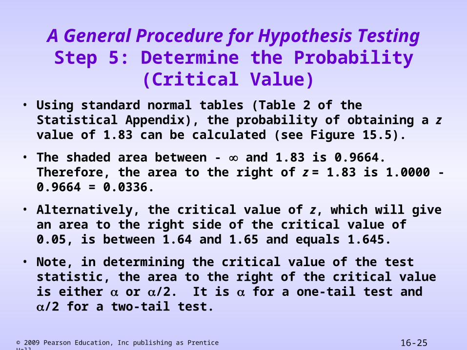
• Using standard normal tables (Table 2 of the Statistical Appendix), the probability of obtaining a z value of 1.83 can be calculated (see Figure 15.5).

• The shaded area between - and 1.83 is 0.9664. Therefore, the area to the right of z = 1.83 is 1.0000 - 0.9664 = 0.0336.

• Alternatively, the critical value of z, which will give an area to the right side of the critical value of 0.05, is between 1.64 and 1.65 and equals 1.645.

• Note, in determining the critical value of the test statistic, the area to the right of the critical value is either or /2. It is for a one-tail test and /2 for a two-tail test.

A General Procedure for Hypothesis TestingStep 5: Determine the Probability (Critical Value)


• If the probability associated with the calculated or observed value of the test statistic (TSCAL) is less than the level of significance (), the null hypothesis is rejected.

• The probability associated with the calculated or observed value of the test statistic is 0.0336. This is the probability of getting a p value of 0.44 when = 0.40. This is less than the level of significance of 0.05. Hence, the null hypothesis is rejected.

• Alternatively, if the absolute calculated value of the test statistic |(TSCAL)| is greater than the absolute critical value of the test statistic |(TSCR)|, the null hypothesis is rejected.

A General Procedure for Hypothesis TestingSteps 6 & 7: Compare the Probability

(Critical Value) and Making the Decision


• The calculated value of the test statistic z = 1.83 lies in the rejection region, beyond the value of 1.645. Again, the same conclusion to reject the null hypothesis is reached.

• Note that the two ways of testing the null hypothesis are equivalent but mathematically opposite in the direction of comparison.

• If the probability of TSCAL < significance level ()

then reject H0 but if |TSCAL | > |TSCR | then reject H0.

A General Procedure for Hypothesis TestingSteps 6 & 7: Compare the Probability (Critical

Value) and Making the Decision (Cont.)


• The conclusion reached by hypothesis testing must be expressed in terms of the marketing research problem.

• In our example, we conclude that there is evidence that the proportion of customers preferring the new plan is significantly greater than 0.40. Hence, the recommendation would be to introduce the new service plan.

A General Procedure for Hypothesis TestingStep 8: Marketing Research Conclusion


Figure 16.9 A Broad Classification of Hypothesis Testing Procedures

Hypothesis Testing

Test of Association Test of Difference

Means Proportions


Cross-Tabulation

• While a frequency distribution describes one variable at a time, a cross-tabulation describes two or more variables simultaneously.

• Cross-tabulation results in tables that reflect the joint distribution of two or more variables with a limited number of categories or distinct values, e.g., Table 16.3.


Table 16.3A Cross-Tabulation of Gender and Usage of Nike Shoes

GENDER

Female Male Row Total

Lights Users 14 5 19

Medium Users 5 5 10

Heavy Users 5 11 16

Column Total 24 21


Two Variables Cross-Tabulation

• Since two variables have been cross classified, percentages could be computed either columnwise, based on column totals (Table 16.4), or rowwise, based on row totals (Table 16.5).

• The general rule is to compute the percentages in the direction of the independent variable, across the dependent variable. The correct way of calculating percentages is as shown in Table 16.4.


Usage

GENDER

Female Male

Light Users 58.4% 23.8%

Medium Users 20.8% 23.8%

Heavy Users 20.8% 52.4%

Column Total 100.0% 100.0%

Table 16.4

Usage of Nike Shoes by Gender


Usage

GENDER

Female Male Raw Total

Light Users 73.7% 26.3% 100.0%

Medium Users 50.0% 50.0% 100.0%

Heavy Users 31.2% 68.8% 100.0%

Table 16.5

Gender by Usage of Nike Shoes


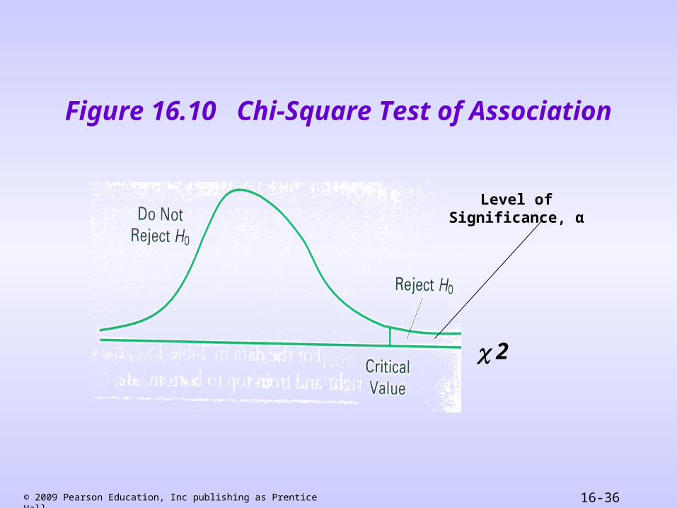
• To determine whether a systematic association exists, the probability of obtaining a value of chi-square as large or larger than the one calculated from the cross-tabulation is estimated.

• An important characteristic of the chi-square statistic is the number of degrees of freedom (df) associated with it. That is, df = (r - 1) x (c -1).

• The null hypothesis (H0) of no association between the two variables will be rejected only when the calculated value of the test statistic is greater than the critical value of the chi-square distribution with the appropriate degrees of freedom, as shown in Figure 16.10.

Statistics Associated with Cross-TabulationChi-Square


Figure 16.10 Chi-Square Test of Association

2

Level of Significance, α



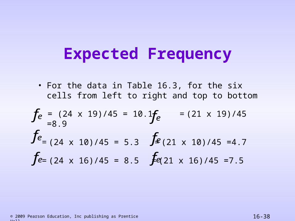
• The chi-square statistic (2) is used to test the statistical significance of the observed association in a cross-tabulation. The expected frequency for each cell can be calculated by using a simple formula:

fe = nrncn

where = total number in the row= total number in the column= total sample size

rncn

n


Expected Frequency

• For the data in Table 16.3, for the six cells from left to right and top to bottom

= (24 x 19)/45 = 10.1 = (21 x 19)/45 =8.9

= (24 x 10)/45 = 5.3 = (21 x 10)/45 =4.7

= (24 x 16)/45 = 8.5 = (21 x 16)/45 =7.5

ef

ef

ef

ef

efef


= (14 -10.1)2 + (5 – 8.9)2

10.1 8.9

+ (5 – 5.3)2 + (5 – 4.7)2

5.3 4.7

+ (5 – 8.5)2 + (11 – 7.5)2

8.5 7.5

= 1.51 + 1.71 + 0.02 + 0.02 + 1.44 + 1.63

= 6.33

2 =(fo - fe)2

feall

cells


• The chi-square distribution is a skewed distribution whose shape depends solely on the number of degrees of freedom. As the number of degrees of freedom increases, the chi-square distribution becomes more symmetrical.

• Table 3 in the Statistical Appendix contains upper-tail areas of the chi-square distribution for different degrees of freedom. For 2 degrees of freedom, the probability of exceeding a chi-square value of 5.991 is 0.05.

• For the cross-tabulation given in Table 16.3, there are (3-1) x (2-1) = 2 degrees of freedom. The calculated chi-square statistic had a value of 6.333. Since this is greater than the critical value of 5.991, the null hypothesis of no association is rejected indicating that the association is statistically significant at the 0.05 level.



• The phi coefficient () is used as a measure of the strength of association in the special case of a table with two rows and two columns (a 2 x 2 table).

• The phi coefficient is proportional to the square root of the chi-square statistic:

• It takes the value of 0 when there is no association, which would be indicated by a chi-square value of 0 as well. When the variables are perfectly associated, phi assumes the value of 1 and all the observations fall just on the main or minor diagonal.

Statistics Associated with Cross-TabulationPhi Coefficient

= 2

n


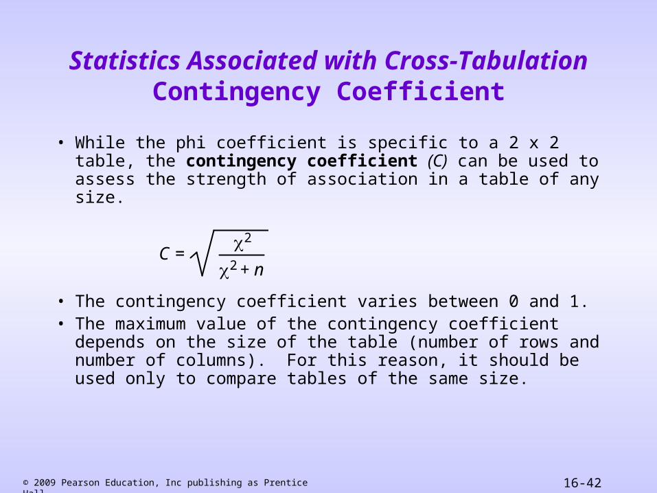
• While the phi coefficient is specific to a 2 x 2 table, the contingency coefficient (C) can be used to assess the strength of association in a table of any size.

• The contingency coefficient varies between 0 and 1. • The maximum value of the contingency coefficient

depends on the size of the table (number of rows and number of columns). For this reason, it should be used only to compare tables of the same size.

Statistics Associated with Cross-TabulationContingency Coefficient

C = 2

2 + n


• Cramer's V is a modified version of the phi correlation coefficient, , and is used in tables larger than 2 x 2.

or

Statistics Associated with Cross-TabulationCramer’s V

V = 2

min (r-1), (c-1)

V = 2/n

min (r-1), (c-1)


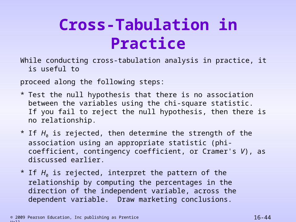
Cross-Tabulation in Practice

While conducting cross-tabulation analysis in practice, it is useful to

proceed along the following steps:

* Test the null hypothesis that there is no association between the variables using the chi-square statistic. If you fail to reject the null hypothesis, then there is no relationship.

* If H0 is rejected, then determine the strength of the association using an appropriate statistic (phi-coefficient, contingency coefficient, or Cramer's V), as discussed earlier.

* If H0 is rejected, interpret the pattern of the relationship by computing the percentages in the direction of the independent variable, across the dependent variable. Draw marketing conclusions.


Construct the Cross-Tabulation Data

Calculate the Chi-Square Statistic, Test the Null Hypothesis of No Association

Reject H0?

Interpret the Pattern of Relationship by Calculating Percentages in the Direction of the Independent Variable

No AssociationDetermine the Strength

of Association Using an Appropriate Statistic

Figure 16.11 Conducting Cross-Tabulation Analysis

NO YES





SPSS Windows: Frequencies • The main program in SPSS is FREQUENCIES. It

produces a table of frequency counts, percentages, and cumulative percentages for the values of each variable. It gives all of the associated statistics.

• If the data are interval scaled and only the summary statistics are desired, the DESCRIPTIVES procedure can be used.

• The EXPLORE procedure produces summary statistics and graphical displays, either for all of the cases or separately for groups of cases. Mean, median, variance, standard deviation, minimum, maximum, and range are some of the statistics that can be calculated.


To select these frequencies procedures, click the following:

• Analyze > Descriptive Statistics > Frequencies . . .

• Or Analyze > Descriptive Statistics > Descriptives . . .

• or Analyze > Descriptive Statistics > Explore . . .

We illustrate the detailed steps using the data of Table 16.1.

SPSS Windows: Frequencies


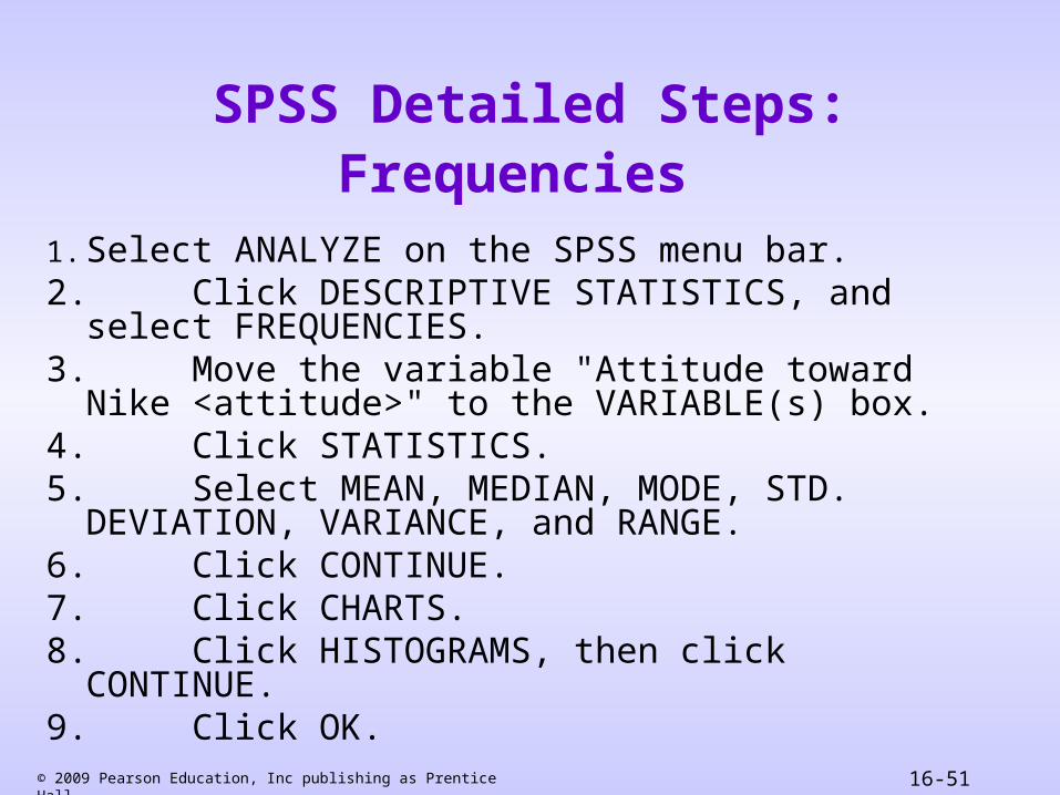
SPSS Detailed Steps: Frequencies

1. Select ANALYZE on the SPSS menu bar.2. Click DESCRIPTIVE STATISTICS, and select

FREQUENCIES.3. Move the variable "Attitude toward Nike <attitude>" to the

VARIABLE(s) box.4. Click STATISTICS.5. Select MEAN, MEDIAN, MODE, STD. DEVIATION,

VARIANCE, and RANGE.6. Click CONTINUE.7. Click CHARTS.8. Click HISTOGRAMS, then click CONTINUE.9. Click OK.


SPSS Windows: Cross-tabulations

The major cross-tabulation program is CROSSTABS. This program will display the cross-classification tables and provide cell counts, row and column percentages, the chi-square test for significance, and all the measures of the strength of the association that have been discussed. To select these procedures, click the following:

• Analyze > Descriptive Statistics > Crosstabs



SPSS Detailed Steps: Cross-Tabulations

1. Select ANALYZE on the SPSS menu bar.2. Click DESCRIPTIVE STATISTICS, and select

CROSSTABS.3. Move the variable "User Group <usergr>" to the ROW(S)

box.4. Move the variable "Sex <sex>" to the COLUMN(S) box.5. Click CELLS.6. Select OBSERVED under COUNTS, and select COLUMN

under PERCENTAGES. 7. Click CONTINUE.8. Click STATISTICS.9. Click CHI-SQUARE, PHI, AND CRAMER'S V.10.Click CONTINUE.11.Click OK.


Excel: Frequencies

The Tools > Data Analysis function computes the descriptive statistics. The output produces the mean, standard error, median, mode, standard deviation, variance, range, minimum, maximum, sum, count, and confidence level. Frequencies can be selected under the histogram function. A histogram can be produced in bar format.



Excel Detailed Steps: Frequencies

1. Select Tools (Alt + T). 2. Select Data Analysis under Tools.3. The Data Analysis Window pops up.4. Select Histogram from the Data Analysis Window.5. Click OK.6. The Histogram pop-up window appears on screen.7. The Histogram window has two portions:

a. Inputb. Output Options:


Excel Detailed Steps: Frequencies (Cont.)

8. Input portion asks for two inputs.a. Click in the input range box and select (highlight) all 45

rows under ATTITUDE. $D$2: $D$46 should appear in the input range box.

b. Do not enter anything into the Bin Range box. (Note that this input is optional; if you do not provide a reference, the system will take values based on range of the data set).

9. In the Output portion of pop-up window, select the following options:a. New Workbook b. Cumulative Percentagec. Chart Output

10.Click OK.


Excel: Cross-Tabulations

The Data > Pivot Table function performs cross-tabulations in Excel. To do additional analysis or customize data, select a different summary function, such as maximum, minimum, average, or standard deviation. In addition, a custom calculation can be selected to analyze values based on other cells in the data plane. ChiTest can be assessed under the Insert > Function > Statistical > ChiTest function.

We illustrate the detailed steps using the data of Table 16.3


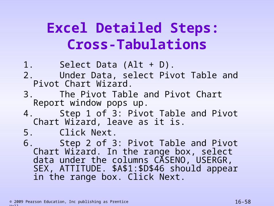
Excel Detailed Steps: Cross-Tabulations

1. Select Data (Alt + D).2. Under Data, select Pivot Table and Pivot Chart

Wizard.3. The Pivot Table and Pivot Chart Report window pops

up.4. Step 1 of 3: Pivot Table and Pivot Chart Wizard,

leave as it is.5. Click Next. 6. Step 2 of 3: Pivot Table and Pivot Chart Wizard. In

the range box, select data under the columns CASENO, USERGR, SEX, ATTITUDE. $A$1:$D$46 should appear in the range box. Click Next.


Excel Detailed Steps: Cross-Tabulations (Cont.)

7. Step 3 of 3: Pivot Table and Pivot Chart Wizard, select New Worksheet in this window. Click Layout and drag the variables in this format.

SEX-------------------------------------|

USERGR | CASENO (Double-click CASENO and select Count)

|8. Click OK and then Finish.


Exhibit 16.1Other Computer Programs: FrequenciesSAS The main program in SAS is UNIVARIATE. In addition to

providing a frequency table, this program provides all of the associated statistics. Another procedure available is FREQ. For one-way frequency distribution, FREQ does not provide any associated statistics. If only summary statistics are desired, procedures such as MEANS, SUMMARY, and TABULATE can be used. It should be noted that FREQ is not available as an independent program in the microcomputer version.

MINITABThe main function is Stats > Descriptive Statistics. The output values include the mean, median, mode, standard deviation, minimum, maximum, and quartiles. A histogram in a bar chart or graph can be produced from the Graph > Histogram selection.


Exhibit 16.2 Other Computer Programs:

Cross-TabulationsSAS

Cross-tabulation can be done by using FREQ. This program will display the cross-classification tables and provide cell counts as well as row and column percentages. In addition, the TABULATE program can be used for obtaining cell counts and row and column percentages, although it does not provide any of the associated statistics.

MINITABIn Minitab, cross-tabulations and chi-square are under the Stats > Tables function. Each of these features must be selected separately under the Tables function.

© 2009 Pearson Education, Inc publishing as Prentice Hall 16-1 Chapter 16 Data Analysis: Frequency Distribution, Hypothesis Testing, and Cross-Tabulation.

Documents

pearson education

frequency analysis slide

frequency histogram

prentice hall

crosstabulation slide

table of frequency counts

nike slide

cross tabulation statistics