© 2002 Prentice-Hall, Inc.Chap 13-1 Statistics for Managers using Microsoft Excel 3 rd Edition Chapter 13 Time Series Analysis.

© 2002 Prentice-Hall, Inc. Chap 13-1

Statistics for Managers using Microsoft Excel

3rd Edition

Chapter 13Time Series Analysis


Chapter Topics

The importance of forecasting Component factors of the time-series

model Smoothing of annual time series

Moving averages Exponential smoothing

Least square trend fitting and forecasting Linear, quadratic and exponential models


Chapter Topics

Autoregressive models Choosing appropriate forecasting

models Time series forecasting of monthly or

quarterly data Pitfalls concerning time-series analysis

(continued)


The Importance of Forecasting

Government needs to forecast unemployment, interest rates, expected revenues from income taxes to formulate policies

Marketing executives need to forecast demand, sales, consumer preferences in strategic planning


The Importance of Forecasting

College administrators need to forecast enrollments to plan for facilities and for faculty recruitment

Retail stores need to forecast demand to control inventory levels, hire employees and provide training

(continued)


Time-Series

Numerical data obtained at regular time intervals

The time intervals can be annually, quarterly, daily, hourly, etc.

Example:Year: 1994 1995 1996 1997

1998Sales: 75.3 74.2 78.5

79.7 80.2


Time-Series Components

Time-Series

Cyclical

Random

Trend

Seasonal


Upward trend

Trend Component

Overall upward or downward movement Data taken over a period of years

Sales

Time


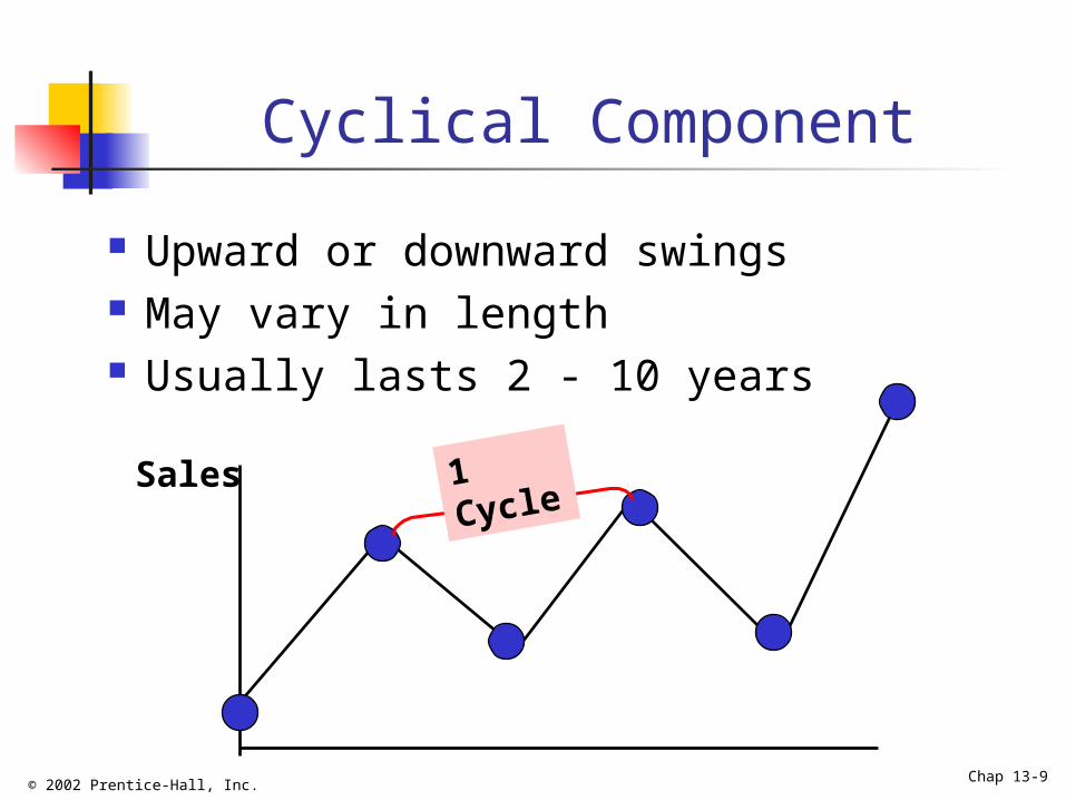
Cyclical Component

Upward or downward swings May vary in length Usually lasts 2 - 10 years

Sales 1 Cycle


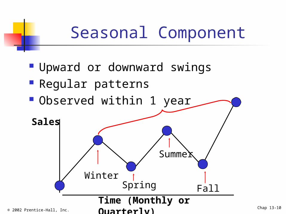
Seasonal Component

Upward or downward swings Regular patterns Observed within 1 year

Sales

Time (Monthly or Quarterly)

WinterSpring

Summer

Fall


Random or Irregular Component

Erratic, nonsystematic, random, “residual” fluctuations

Due to random variations of Nature Accidents

Short duration and non-repeating


e.g.: Quarterly Retail Sales with Seasonal Components

Quarterly with Seasonal Components

0

5

10

15

20

25

0 5 10 15 20 25 30 35

Time

Sale

s


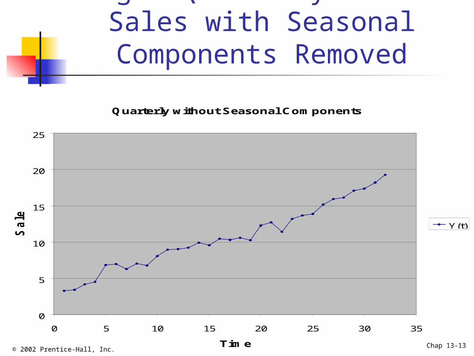
e.g.: Quarterly Retail Sales with Seasonal Components

Removed

Quarterly without Seasonal Components

0

5

10

15

20

25

0 5 10 15 20 25 30 35

Time

Sa

les

Y(t)


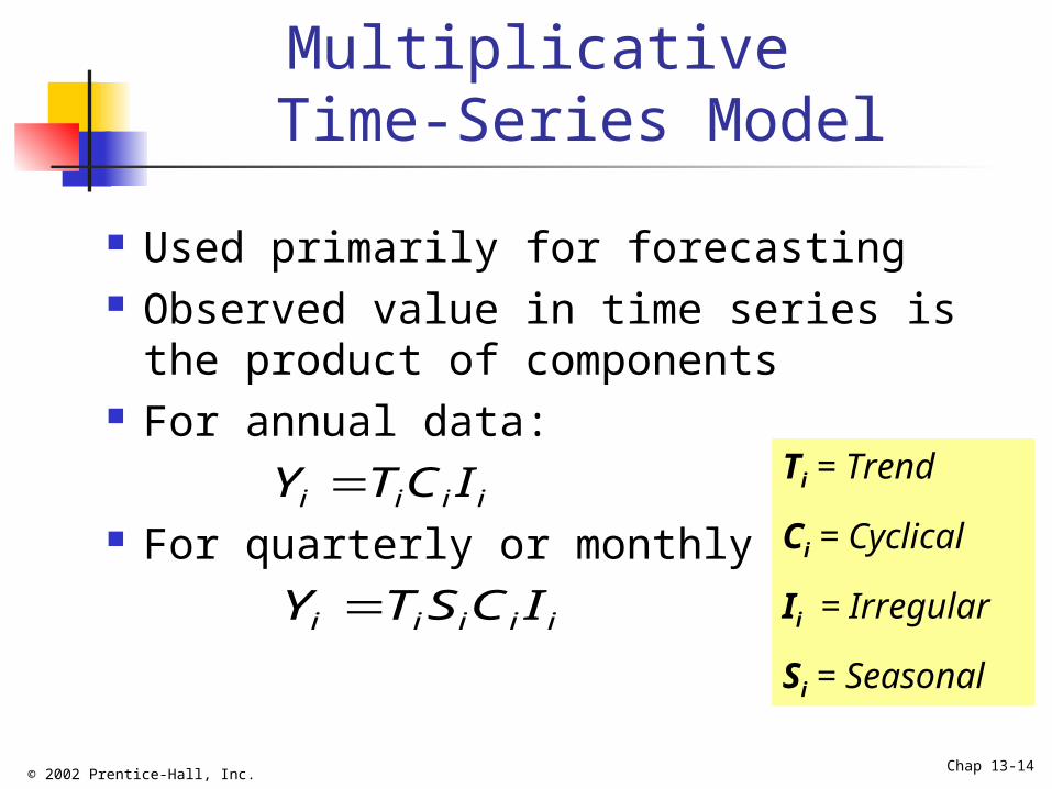
Multiplicative Time-Series Model

Used primarily for forecasting Observed value in time series is the

product of components For annual data:

For quarterly or monthly data:

Ti = Trend

Ci = Cyclical

Ii = Irregular

Si = Seasonal

i i i i iY T S C I

i i i iY TC I


Moving Averages

Used for smoothing Series of arithmetic means over time Result dependent upon choice of L

(length of period for computing means) To smooth out cyclical component, L

should be multiple of the estimated average length of the cycle

For annual time-series, L should be odd


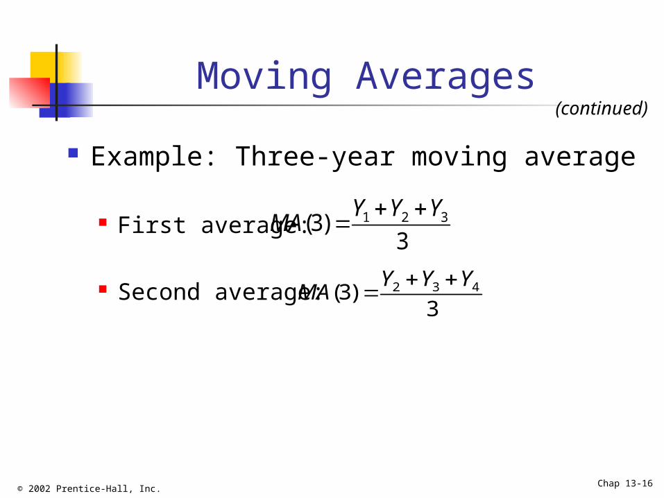
Moving Averages

Example: Three-year moving average

First average:

Second average:

1 2 3(3)3

Y Y YMA

2 3 4(3)3

Y Y YMA

(continued)


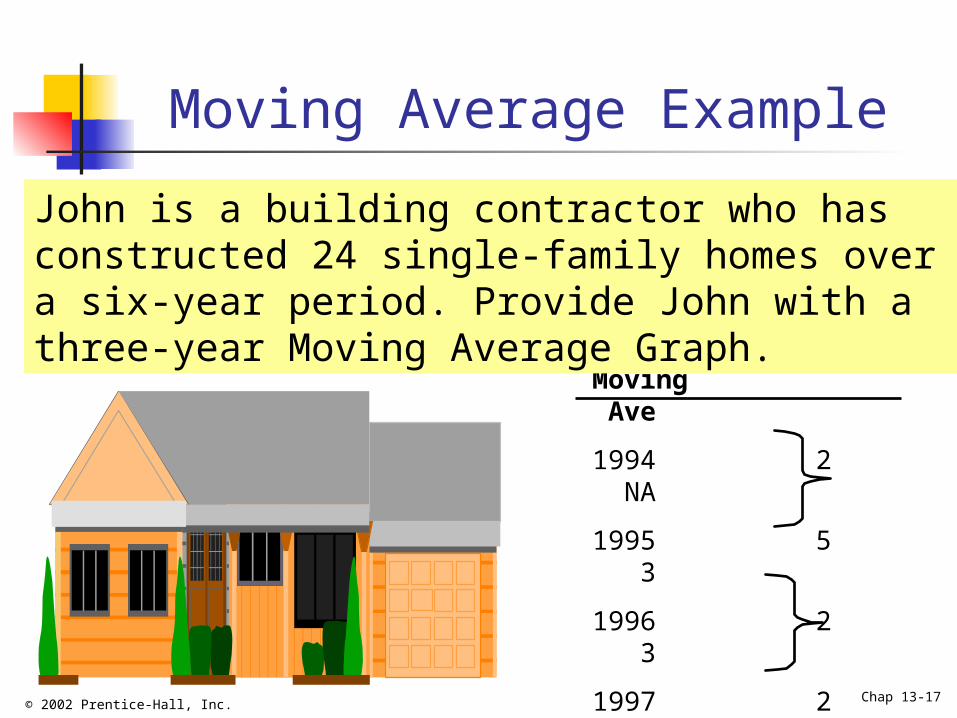
Moving Average Example

Year Units Moving Ave

1994 2 NA

1995 5 3

1996 2 3

1997 2 3.67

1998 7 5

1999 6 NA

John is a building contractor who has constructed 24 single-family homes over a six-year period. Provide John with a three-year Moving Average Graph.


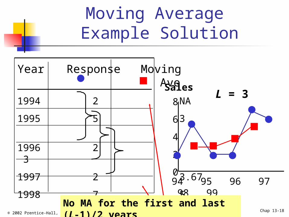
Moving Average Example Solution

Year Response Moving Ave

1994 2 NA

1995 5 3

1996 2 3

1997 2 3.67

1998 7 5

1999 6 NA94 95 96 97 98 99

8

6

4

2

0

SalesL = 3

No MA for the first and last (L-1)/2 years


Moving Average Example Solution in Excel

Use excel formula “=average (cell range containing the data for the years to average)”

Excel spreadsheet for the single family home sales example

Microsoft Excel Worksheet


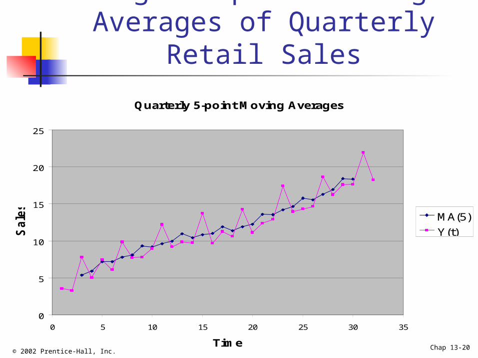
e.g.: 5-point Moving Averages of Quarterly Retail

Sales

Quarterly 5-point Moving Averages

0

5

10

15

20

25

0 5 10 15 20 25 30 35

Time

Sale

s

MA(5)

Y(t)


Exponential Smoothing Weighted moving average

Weights decline exponentially Most recent observation weighted most

Used for smoothing and short term forecasting

Weights are: Subjectively chosen Ranges from 0 to 1

Close to 0 for smoothing out unwanted cyclical and irregular components

Close to 1 for forecasting


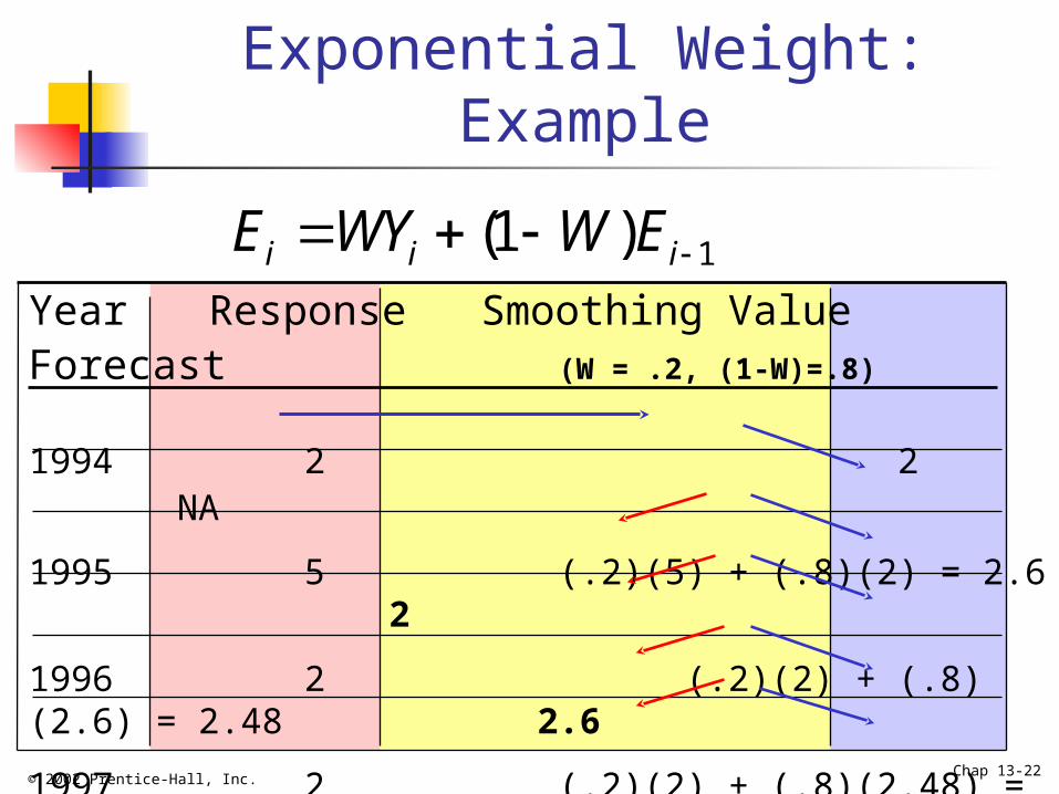
Exponential Weight: Example

Year Response Smoothing Value Forecast(W = .2, (1-W)=.8)

1994 2 2 NA

1995 5 (.2)(5) + (.8)(2) = 2.6 2

1996 2 (.2)(2) + (.8)(2.6) = 2.48 2.6

1997 2 (.2)(2) + (.8)(2.48) = 2.384 2.48

1998 7 (.2)(7) + (.8)(2.384) = 3.307 2.384

1999 6 (.2)(6) + (.8)(3.307) = 3.846 3.307

1(1 )i i iE WY W E


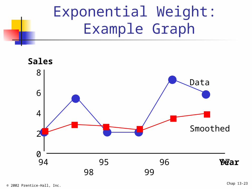
Exponential Weight: Example Graph

94 95 96 97 98 99

8

6

4

2

0

Sales

Year

Data

Smoothed


Exponential Smoothing in Excel

Use tools | data analysis | exponential smoothing The damping factor is (1-W )




Example: Exponential Smoothing of Real GNP

The EXCEL spreadsheet with the real GDP data and the exponentially smoothed series



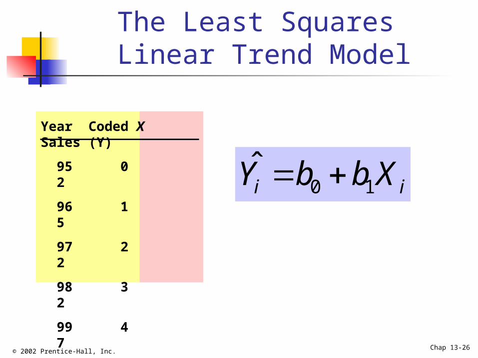
The Least Squares Linear Trend Model

Year Coded X Sales (Y)

95 0 2

96 1 5

97 2 2

98 3 2

99 4 7

00 5 6

0 1i iY b b X


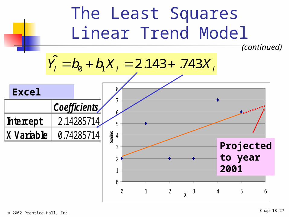
The Least Squares Linear Trend Model

(continued)

0 1ˆ 2.143 .743i i iY b b X X

Excel Output

CoefficientsIntercept 2.14285714X Variable 1 0.74285714

0

1

2

3

4

5

6

7

8

0 1 2 3 4 5 6X

Sale

s

Projected to year 2001


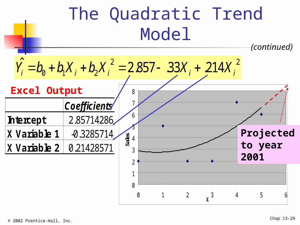
The Quadratic Trend Model

20 1 2i i iY b b X b X


95 0 2

96 1 5

97 2 2

98 3 2

99 4 7

00 5 6


2 20 1 2

ˆ 2.857 .33 .214i i i i iY b b X b X X X

The Quadratic Trend Model(continued)

CoefficientsIntercept 2.85714286X Variable 1 -0.3285714X Variable 2 0.21428571

Excel Output

0

1

2

3

4

5

6

7

8

0 1 2 3 4 5 6 X

Sale

s Projected to year 2001


The Exponential Trend Model

CoefficientsIntercept 0.33583795X Variable 10.08068544

0 1ˆ iXiY b b or

Excel Output of Values in logs

ˆ (2.17)(1.2) iXiY

antilog(.33583795) = 2.17antilog(.08068544) = 1.2

0 1 1ˆlog log logiY b X b


95 0 2

96 1 5

97 2 2

98 3 2

99 4 7

00 5 6


The Least Squares Trend Models in PHStat

Use PHStat | simple linear regression for linear trend and exponential trend models and PHStat | multiple regression for quadratic trend model




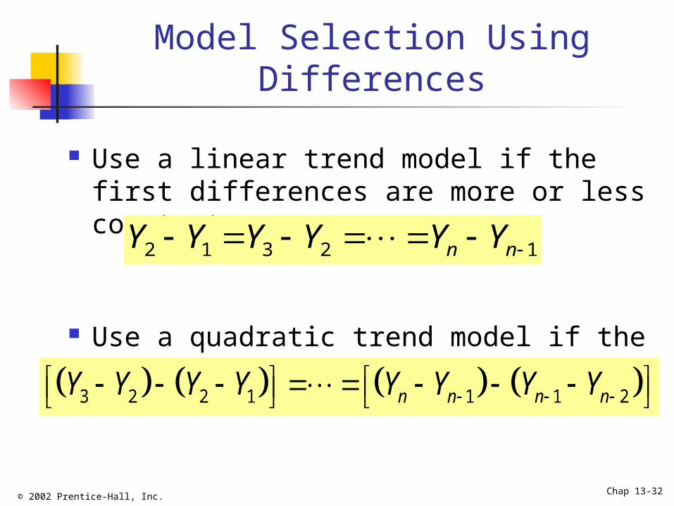
Model Selection Using Differences

Use a linear trend model if the first differences are more or less constant

Use a quadratic trend model if the second differences are more or less constant

2 1 3 2 1n nY Y Y Y Y Y

3 2 2 1 1 1 2n n n nY Y Y Y Y Y Y Y


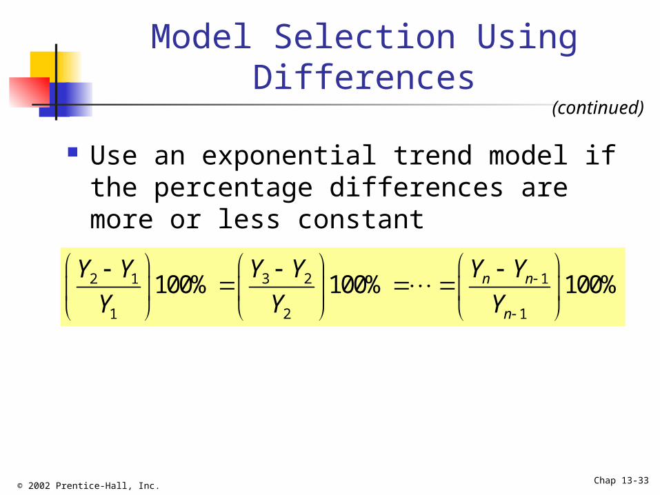
Model Selection Using Differences

3 2 12 1

1 2 1

100% 100% 100%n n

n

Y Y Y YY Y

Y Y Y

Use an exponential trend model if the percentage differences are more or less constant

(continued)


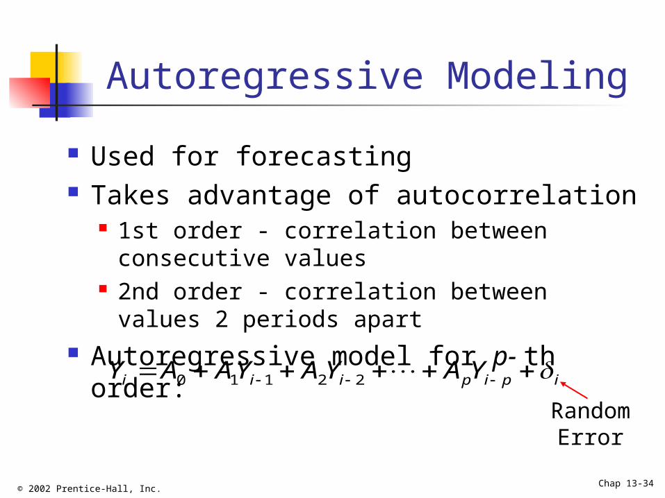
Autoregressive Modeling

Used for forecasting Takes advantage of autocorrelation

1st order - correlation between consecutive values

2nd order - correlation between values 2 periods apart

Autoregressive model for p- th order:

Random Error

0 1 1 2 2i i i p i p iY A AY A Y A Y


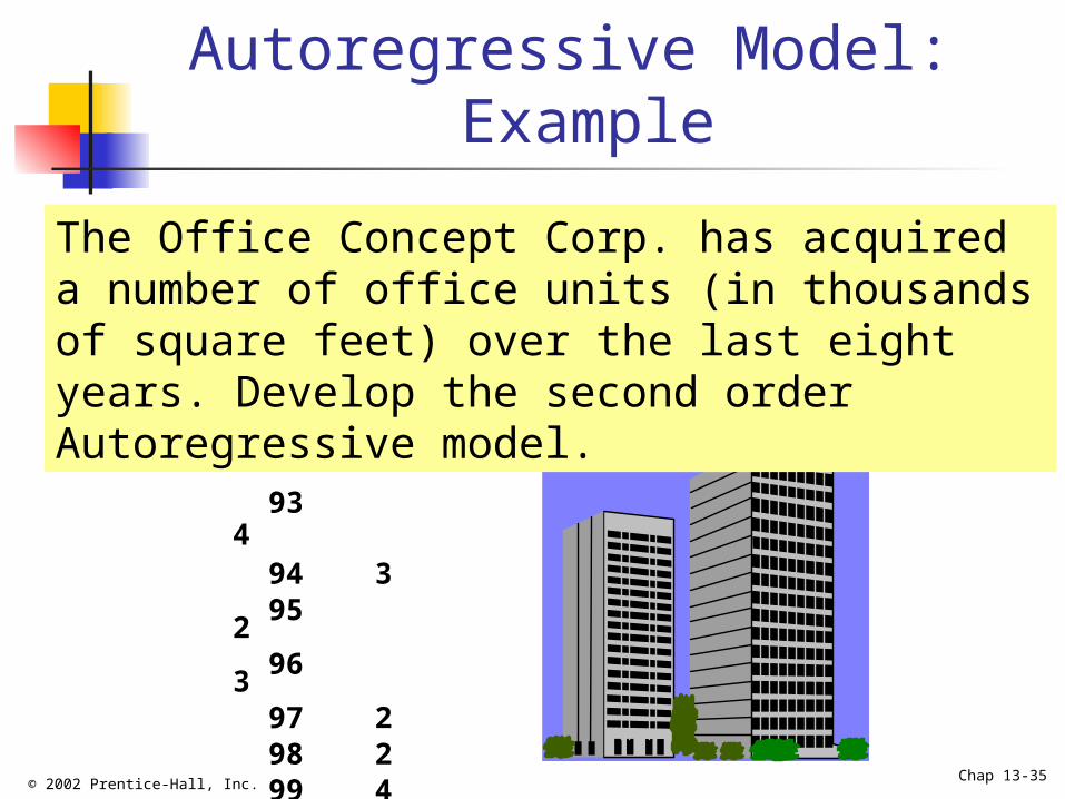
Autoregressive Model: Example

Year Units

93 4 94 3 95 2 96 3 97 2 98 2 99 4 00 6

The Office Concept Corp. has acquired a number of office units (in thousands of square feet) over the last eight years. Develop the second order Autoregressive model.


Autoregressive Model: Example Solution

Year Yi Yi-1 Yi-2

93 4 --- --- 94 3 4 --- 95 2 3 4 96 3 2 3 97 2 3 2 98 2 2 3 99 4 2 2 00 6 4 2

CoefficientsIntercept 3.5X Variable 1 0.8125X Variable 2 -0.9375

Excel Output

1 2ˆ 3.5 .8125 .9375i i iY Y Y

Develop the 2nd order table

Use Excel to estimate a regression model


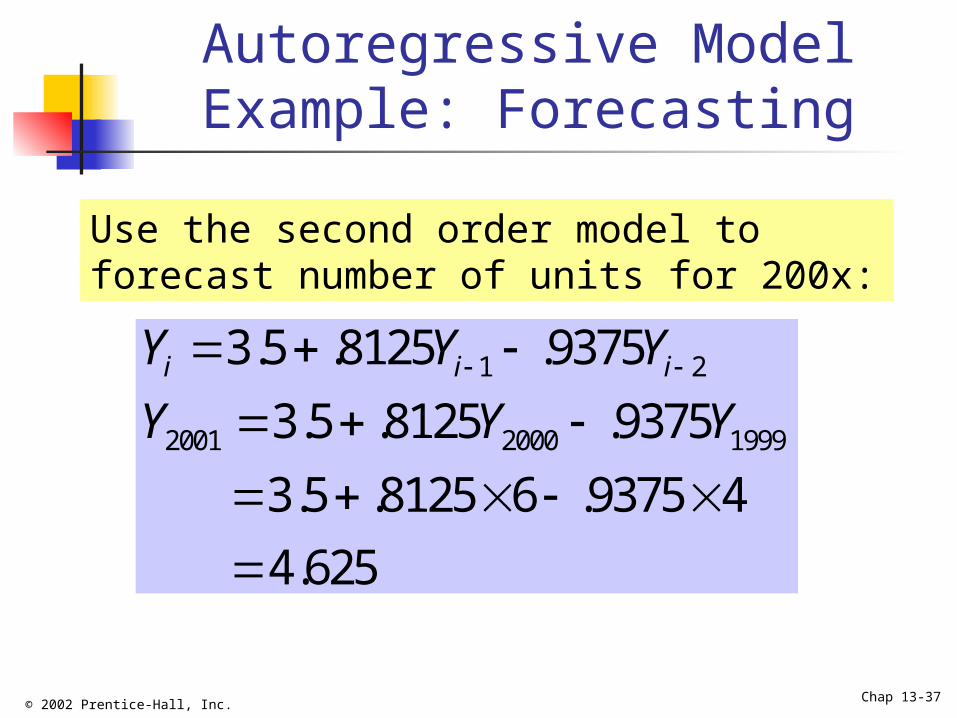
Autoregressive Model Example: Forecasting

Use the second order model to forecast number of units for 200x:

1 2

2001 2000 1999

3.5 .8125 .9375

3.5 .8125 .9375

3.5 .8125 6 .9375 4

4.625

i i iY Y Y

Y Y Y


Autoregressive Model in PHStat

PHStat | multiple regression

Excel spreadsheet for the office units example



Autoregressive Modeling Steps

1. Choose p : note that df = n - 2p - 12. Form a series of “lag predictor” variables

Yi-1 , Yi-2 , … ,Yi-p

3. Use excel to run regression model using all p variables

4. Test significance of Ap

If null hypothesis rejected, this model is selected

If null hypothesis not rejected, decrease p by 1 and repeat


Selecting A Forecasting Model

Perform a residual analysis Look for pattern or direction

Measure sum of square error - SSE (residual errors)

Measure residual error using MAD Use simplest model

Principle of parsimony


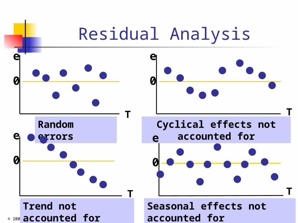
Residual Analysis

Random errors

Trend not accounted for

Cyclical effects not accounted for

Seasonal effects not accounted for

T T

T T

e e

e e

0 0

0 0


Measuring Errors

Choose a model that gives the smallest measuring errors

Sum square error (SSE)

Sensitive to outliers

2

1

ˆn

i ii

SSE Y Y


Measuring Errors

Mean Absolute Deviation (MAD)

Not sensitive to extreme observations

(continued)

1

ˆn

i ii

Y YMAD

n


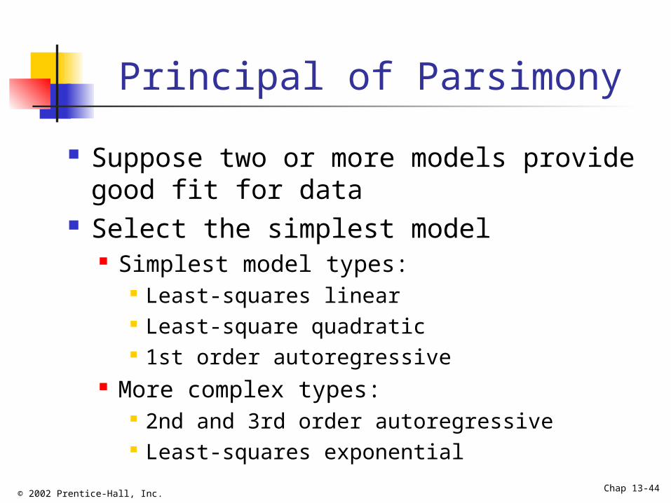
Principal of Parsimony

Suppose two or more models provide good fit for data

Select the simplest model Simplest model types:

Least-squares linear Least-square quadratic 1st order autoregressive

More complex types: 2nd and 3rd order autoregressive Least-squares exponential


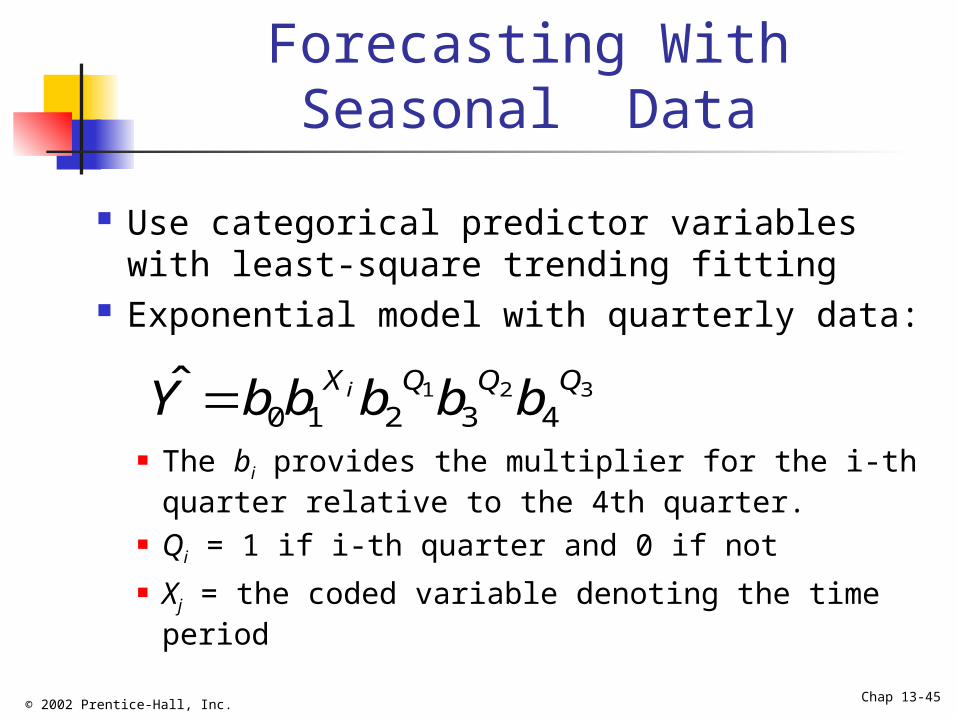
Forecasting With Seasonal Data

Use categorical predictor variables with least-square trending fitting

Exponential model with quarterly data:

The bi provides the multiplier for the i-th quarter relative to the 4th quarter.

Qi = 1 if i-th quarter and 0 if not Xj = the coded variable denoting the time

period

1 2 3

0 1 2 3 4ˆ iX Q Q QY b b b b b


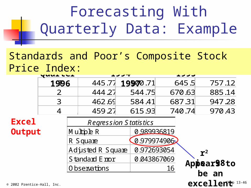
Forecasting With Quarterly Data: Example

445.77444.27462.69459.27

500.71544.75584.41615.93

645.5670.63687.31740.74

757.12885.14947.28970.43

I234

Quarter 1994 1995 1996 1997

Standards and Poor’s Composite Stock Price Index:

Excel Output

Appears to be an excellent fit.

r2 is .98

Regression StatisticsMultiple R 0.989936819R Square 0.979974906Adjusted R Square 0.972693054Standard Error 0.043867069Observations 16


Forecasting With Quarterly Data: Example

(continued)

Excel Output

0 1 1 2

1

ˆln ln ln ln

6.011 .0553 0.0104i i

i

Y b X b Q b

X Q

Regression Equation for the first quarter:

Coefficients Standard ErrorIntercept 6.011187697 0.031115484Coded X 0.055372493 0.002452244Q1 0.010421639 0.031879168Q2 0.023885562 0.031404042Q3 0.019342411 0.031115484


Forecasting with Quarterly Data in PHStat

Use PHStat | multiple regression

Excel spreadsheet for the stock price index example



Pitfalls Regarding Time-Series Analysis

Assuming the mechanism that governs the time series behavior in the past will still hold in the future

Using mechanical extrapolation of the trend to forecast the future without considering personal judgments, business experiences, changing technologies, and habits, etc.


Chapter Summary

Discussed the importance of forecasting Addressed component factors of the

time-series model Performed smoothing of data series

Moving averages Exponential smoothing

Described least square trend fitting and forecasting Linear, quadratic and exponential models


Chapter Summary

Addressed autoregressive models Described procedure for choosing

appropriate models Addressed time series forecasting of

monthly or quarterly data (use of dummy variables)

Discussed pitfalls concerning time-series analysis

(continued)

© 2002 Prentice-Hall, Inc.Chap 13-1 Statistics for Managers using Microsoft Excel 3 rd Edition Chapter 13 Time Series Analysis.

Documents

time series analysis

annual time series

annual timeseries

timeseries analysis

cycle slide

timeseries numerical

odd slide

year sales time monthly