USING OF POLAR CODES IN STEGANOGRAPHY
I. DIOP; S .M FARSSI; B. DIOUF; H .B DIOUF
Polytechnic school of Cheikh Anta Diop University Dakar Senegal;
email:[email protected]; [email protected]
ABSTRACT: Steganography is the art of secret
communication. Since the advent of modern steganography, in the
2000s, many approaches based on error correcting
codes (Hamming, BCH, RS, STC ...) have been proposed to
reduce the number of changes in the roof while inserting
the maximum bit.
In this paper we propose a new steganography scheme based on
the polar codes. The scheme works according to two steps. The
first offers a stego vector from given cover vector and message.
The stego vector provided by the first method can be the optimal;
in this case the insertion is successful with a very low complexity.
Otherwise, we formalize our steganography problem in a linear
program form with initial solution the stego vector given by the
first method to converge to the optimal solution. Our scheme
works with the case of a constant profile as well with any profile;
it is then adapted to the case of wet papers. Tests of the scheme on
multiple images in gray scale have showed its good performance
in terms of minimizing the embedding impact.
KEYWORDS: STEGANOGRAPHY, MATRIX EMBEDDING, POLAR CODES,
LINEAR PROGRAMMING, WET PAPER CODES
1 INTRODUCTION
The steganography is a technique allowing hiding an
information in a medium (image, sound or video)
unsuspected so that it was undetectable. To reach this
objective it is indispensable to use a technique in order to
reduce the distortion induced by the hiding of the secret
message. The matrix embedding technique introduced by
Crandall [1] has allowed the definition of steganography
schemes that minimize the embedding impact. The first
implementation was created with the work of Westfeld [2]
in which the Hamming code has been used. Afterwards the
BCH codes [3, 4], the Reed-Solomon codes [5] and the
STC codes [6] are used in steganography. The combination
of the techniques of LSB, of matrix embedding and wet
paper has allowed realizing more effective and more
reliable steganography schemes. Our works is a
contribution of schemes of minimization of embedding
impact. We propose in this paper a new steganography
scheme based on the polar codes. The scheme is applied to
the cases of constant profile and of wet paper.
This paper is organized as following. Section 1 describes
the concepts of matrix embedding and minimization of
embedding impact. In Section 3 we study the linear
programming. The polar codes used for the implementation
of our scheme are presented in Section 4. In Section 5 we
propose our scheme based on the polar codes. Section 6
show the results obtained when the scheme is applied on
images. Explications of these results are also given in this
Section. Section 7 concludes the paper.
2 STEGANOGRAPHY AND MATRIX EMBEDDING
2.1 Steganography
Steganography or the art of secret communication aims
to hide a message in an apparently innocuous cover
medium.
Steganography schemes are characterized by different
parameters. The insertion capacity represents the maximum
number of bits that can be inserted in a cover medium. The
rate is the number of bits of the message by inserted support
element and the change density defines the proportion of
modified components of the cover. The embedding
efficiency is the number of bits of the message by distortion
unit. This is the ratio of the rate by the density change. This
last characteristic is used to evaluate the performance of a
steganography scheme. We say that a steganography
scheme is even better than its insertion efficiency is great.
2.2 Distortion measure with the PSNR
The PSNR (Peak Signal Noise Ratio) is a distortion
measure between two images. It is calculate from MSE
(Mean Square Error) and is expressed in . Let and
be respectively the images original and reconstructed
images of same length .
The PSNR and the MSE are given by:
( )
( ) ( )
( )
∑∑ ( ) ( )
( )
where is the dynamic (the maximum value of a pixel).
If the pixels are coded with bits .
2
More the value of PSNR is greater; more the images
compared are similar. A PSNR of more than 35 dB
between two images means that there is no visible
difference between these two images [7]. If the PSNR is
less than 20 dB the two images are very different.
2.3 The principle of matrix embedding
Consider the cover vector consists of the LSBs of the
cover image, the stego vector , the vector of changes
( ), the secret message and the parity check
matrix correcting code errors used. The principle of
matrix embedding is to find the stego vector closest to
such that . By replacing by we will have
.
The objective of the sender is to find the vector of
minimum weight in the coset ( ) (the set of the
vectors of size and syndrome ) and then add it
with to find . At the reception, to find , the decoding is
just done by the matrix product .
2.4 Minimization of embedding impact
We still consider the vectors defined above. Assuming
that the changes do not interact with each other, the total
embedding impact is the sum of the embedding impact at
each pixel [6]:
( ) ∑ | |
( )
with the cost the change of the pixel into
. The goal is for the sender to insert its binary message
so that the distortion is minimized.
The functions of insertion and extraction are defined by:
( ) ( )
( ) ( )
( ) ( )
where ( ) is a parity check matrix of the
code ( ) and ( ) | is the
coset corresponding to the syndrome .
3 LINEAR PROGRAMMING
The linear programming is a central domain of
optimization. An optimization problem highlights variables,
constraints on these variables and a criterion to optimize. It
can be formulated as follows:
( )
with s.t : subject to, the criterion to optimize (objective
function), the variable and the set of constraints
(feasible set).
A linear program can be written either in the canonical
form or in the standard form (obtained from the canonical
form).
Canonical form Standard form
( )
{
( )
{
Before solving a linear programming problem, we must
begin by putting it in standard form with the introduction of
discard variables that allow setting the expression of
constraints in the form of a linear equations system. The
solving of a linear program can be done by using the
simplex method or methods of interior points.
3.1 Simplex Method
This method was developed in the late 40s by G. Danzig
and solves linear programs. To avoid calculating the
solutions of all linear systems extracts from , we
may use the simplex algorithm. This algorithm is based on
the following approach presented in [8]: starting from a
vertex representing the initial solution, we traverse the
whole of the vertices of the set of feasible solutions (a
polyhedron) by determining if the current vertex is optimal
and if not the case, we move to adjacent vertex that
optimizes the objective function. Starting of a vertex
representing the initial solution, we move from extreme
point (vertex) to extreme point along the frontier of the
polyhedron and since the number of extreme points is finite,
the algorithm is called combinatory.
3.2 Methods of interiors points
The 1984 publication of the work of Karmarkar [9] gave
rise to interior point methods which are intended to reduce
the complexity observed in the simplex algorithm. The
interior point methods start from an interior point (initial
solution) to the domain of feasible solutions, then using a
fixed strategy determines an approximate value of the
optimal solution [10]. The movement is made along the
direction that gives the best qualifying improvement of the
objective function. In general, the direction is inside the
polyhedron and the method is called "nonlinear". The
3
advantages of these methods compared to the simplex
method are robustness, polynomial complexity and fast
convergence to the real problems of large sizes.
Clearly, a method of solving a linear program is even
faster than the initial solution is close to the optimal value
sought. We will see in Section 7 that our optimization
problem is particular.
4 THE POLARS CODES
4.1 Usual notations
Let the channel B-DMC (Binary input-
Discrete Memoryless Channel) on which the transmission
takes place. The sets and respectively represent the
input and output alphabets of the channel . ( | ) is the
transition probability such that and The
channel correspond to uses of . The operation
defines the modulo-2 addition and Kronecker product.
denote the line vector ( ) where ,
being a positive integer. is the subvector off indices
( ) and those of even indices ( ) .
4.2 Definitions
The symmetric capacity (bits/s) of the channel B-DMC
is defined as following [11]:
( ) ∑ ∑
( | )
( | )
( | )
( | ) ( )
and Bhattacharyya parameter or reliability of the channel
is given by:
( ) ∑ √ ( | ) ( | )
( )
The polar coding is based on these two parameters.
Two types of usual symmetrical channels are Binary
Erasure Channel (BEC) and Binary Symmetric Channel
(BSC). A B-DMC channel is a BSC if , ( | ) ( | ) and ( | ) ( | ) and a BEC if
( | ) ( | ) or ( | ) ( | )
For any B-DMC , we have [11]:
( ) ( ) √ ( ) ( )
( ) ( ) ( ) ( ) ( )
The parameters ( ) and ( ) take their values in
and more verify the following equivalences:
( ) is equivalent to ( ) and (perfect canal)
( ) is equivalent to ( ) (completely noisy)
From these two equivalences we can say that, to know
the properties of a B-DMC channel, it suffices to study one
of the two parameters. The larger ( ) is the better is the
channel and vice versa. On the other hand the channel with
the smallest value of ( ) is the most reliable. We will
focus particularly on ( ) more easy to manipulate
4.3 Channel polarization and transformation
4.3.1 Channel polarization
Polarization constitutes the base of the construction of
polar codes. It consists in synthesizing of independent
copies of a given B-DMC n other channels to create
others ( ) . The polarization appears in the
sense that ( ( )) tends to 0 or 1 depending on whether
( ( )
) is closer to 0 or 1. The operation of channel
polarization is constituted of two steps: the channels
combination and channel splitting.
4.3.1.1 The channels combination
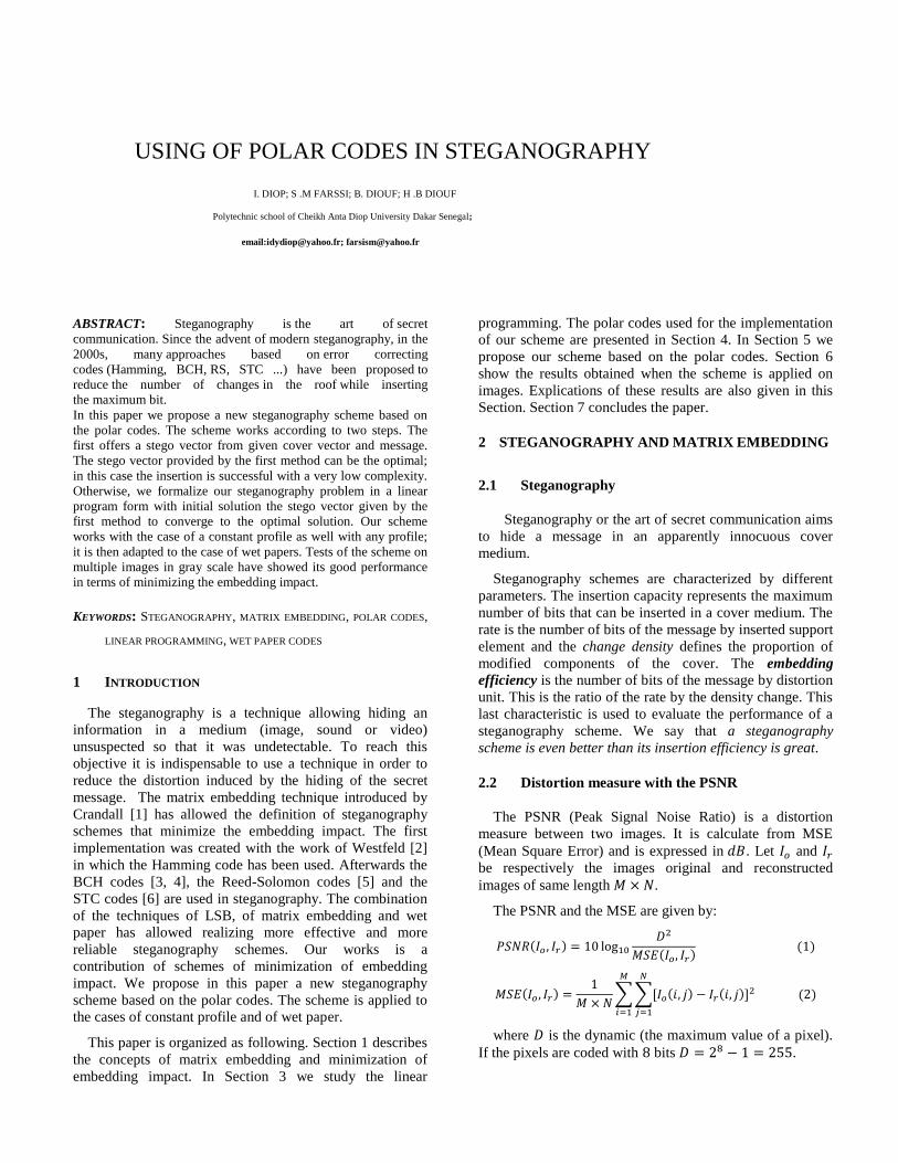
This is to group copies of a given B-DMC channel
in a given channel . The combination for the level
associed independent copies of to
form the channel .
Figure 1: Construction of the channel .
The following relations are established from Figure 1:
and . Thus and
are linked by
the relation
with =[
].
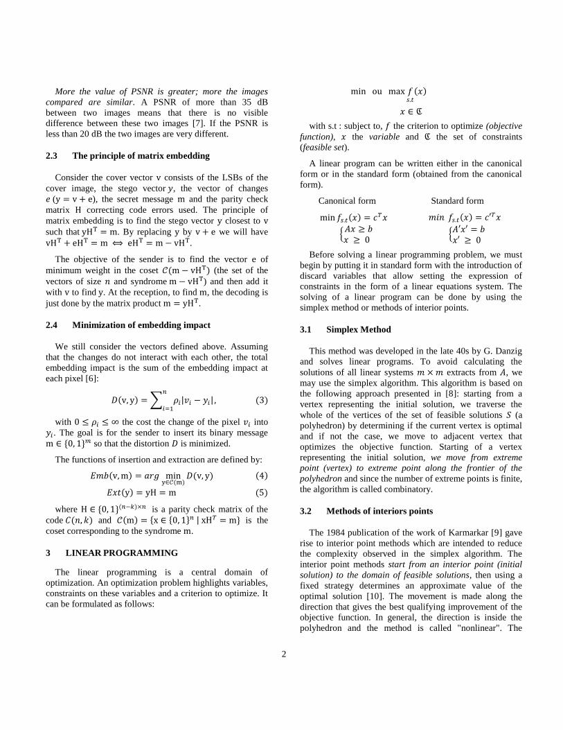
The generalization of the channels combination
procedure with any ( ) is given by a
combination of two independent copies of the channel
to form . The first step is the passage from the input
of to such that and for
. The permutation matrix transforms
into (
), the input for the two copies of .
4
Figure 2: Construction of the channel from two copies of
.
The relation of polar coding is
( )
The matrix
is called generator matrix, a
permutation matrix and
the product of Kronecker of
copies of a matrix .
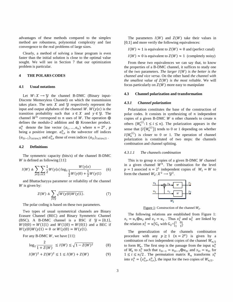
4.3.1.2 The channel splitting
After the channels combination the next step of the
channel polarization is to subdivide the channel into
channel ( )
defined by the following
transition probabilities:
( )(
| ) ∑
(
| )
If is uniform on then
( ) is the channel really
seen by ; all happens as if each input bit borrows the
channel ( )
to give (
) as shown in Figure 3.
Figure 3: Equivalent scheme of polar coding.
4.3.2 The recursive channel transformation
The process of transformation can be generalized
recursively:
( ( )
( )
) ⃗⃗ ⃗⃗ ⃗⃗ ⃗⃗ ⃗⃗ ⃗⃗ ⃗⃗ ⃗⃗ ⃗⃗ ⃗⃗ ⃗⃗ ⃗⃗ ⃗⃗ ⃗⃗ ⃗⃗ ⃗⃗ ⃗⃗ ⃗⃗ ⃗⃗ ⃗( ( )
( )
)
The recurrence relations used for the construction of the
polar codes are [11]:
( ( )
) ( ( )) (
( )) ( )
( ( )) (
( )) ( )
with equality if is a BEC.
These two relations will be used for the construction of
polar codes in Section 6.
4.4 The polar coding
The principle of polar coding is to create a system of
coding allowing to access to each channel ( )
individually
and send the data through those more reliable that is to say
those for which ( ( )
) is more near to 0.
Consider a given subset of dimension and his et son
complementary in . We will fixe ( is also
fixed) and by letting variable. The vector is
called information vector and frozen vector (its bits are
fixed). In general we choose because the choice
of don’t affect the performances of a symmetric channel
[11]. The set is chosen such that ( ( )
) ( ( )
) for
any and .
4.4.1 The construction of polar codes
To construct a polar code we need as inputs the channel
B-DMC on which the code is applied, the block length
and dimension of the code. The algorithm of construction
provide as output the information set of size
such that the value of ∑ ( ( )
) is minimal.
4.4.2 Polar encoding
We use the relation ( ) for encode a data word in a
codeword . An interpretation of the various operations of
permutation which consists gives us the following
expression [11]:
( ⁄ )
( )
with a permutation matrix defined by:
( ⁄ )( ⁄ ) ( ⁄ )
5
( ⁄ ) ( )
From these two relations we try to define more explicitly
the permutation matrices and . For this we will use
the indicial notation of the vectors.
Let be a vector then the element is noted by
where correspond to the binary
representation of .
The matrix acts on a vector by performing a
cyclic shift of index bits to the left. For example if
then
.
The permutation matrix , consisting of shift
matrices, performs cyclic shifts to the left in accordance
with the following process: for the shift we consider
the first bits from the left to the right. That is to
reverse the order of index bits. If
we have
.
We will use in our practical part (Section 5) recursion
formulas (11) and (12) to find the permutation matrix
and the generator matrix of the polar code.
4.4.3 The decoding of polar codes
Several types of decoding of polar codes exist namely
Successive Cancellation (SC) [11], the Linear Programming
(LP) decoding [12] and Belief Propagation (BP) decoding,
etc. Among these types of decoding the most powerful is
the SC but because of the probability of the channels
involved in its implementation its application in
steganography is not yet possible. Therefore we use the LP
decoding for the formulation of our steganographic scheme.
5 STEGANOGRAPHIC SCHEMA BASED ON
POLAR CODES
Before defining the scheme we describe first the
construction of polar codes in the steganographic context.
5.1 The different steps of the construction of polar
codes for the steganography
The construction of the polar codes for the steganography
can be summed up in true steps as shown by Figure 4.
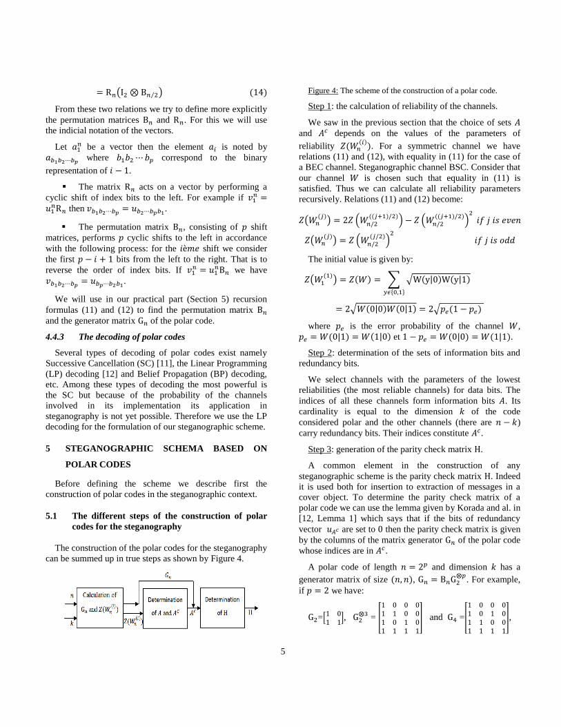
Figure 4: The scheme of the construction of a polar code.
Step 1: the calculation of reliability of the channels.
We saw in the previous section that the choice of sets
and depends on the values of the parameters of
reliability ( ( )). For a symmetric channel we have
relations (11) and (12), with equality in (11) for the case of
a BEC channel. Steganographic channel BSC. Consider that
our channel is chosen such that equality in (11) is
satisfied. Thus we can calculate all reliability parameters
recursively. Relations (11) and (12) become:
( ( )
) ( (( ) )
) ( (( ) )
)
( ( )
) ( ( )
)
The initial value is given by:
( ( )
) ( ) ∑ √ ( | ) ( | )
√ ( | ) ( | ) √ ( )
where is the error probability of the channel ,
( | ) ( | ) et ( | ) ( | ).
Step 2: determination of the sets of information bits and
redundancy bits.
We select channels with the parameters of the lowest
reliabilities (the most reliable channels) for data bits. The
indices of all these channels form information bits . Its
cardinality is equal to the dimension of the code
considered polar and the other channels (there are )
carry redundancy bits. Their indices constitute .
Step 3: generation of the parity check matrix .
A common element in the construction of any
steganographic scheme is the parity check matrix . Indeed
it is used both for insertion to extraction of messages in a
cover object. To determine the parity check matrix of a
polar code we can use the lemma given by Korada and al. in
[12, Lemma 1] which says that if the bits of redundancy
vector are set to then the parity check matrix is given
by the columns of the matrix generator of the polar code
whose indices are in .
A polar code of length and dimension has a
generator matrix of size ( ),
. For example,
if we have:
=[
], = [
] and =[
],
6
where is the matrix that permute lines and of .
The calculation of the reliability parameters give
( ( )
) , ( ( )
) ,
( ( )
) and ( ( )
) .
( ( )
) ( ( )
) ( ( )
) ( ( )
).
If we choose , one canal will be used for the
information then and . The parity
check matrix will be defined as following:
= [
] and = [
]
5.2 Steganography scheme with a polar code
In this party of the paper we consider that the change of
any pixel produces the same distortion (constant profile).
Thus we are interested in the number of bits changed during
insertion. The research of the stego vector will follow two
phases.
5.2.1 First method proposed
We will draw our inspiration from the work of Fridrich
and al. [6] in which the proposed steganography scheme is
strongly related to the form of the parity check matrix of the
STC code used. Indeed, by observing the parity check
matrix of polar code and its transpose , we can make
the following remarks:
1) the columns of are pairwise independent;
2) if we scan the columns of , the position at
which it meets the first non-zero coefficient (equal to )
differs from that of other columns of ;
3) more starting from the last column and starting
with the first line, the position at which we meets the first
non-zero coefficient is the first met on this line; so, the last
position equal to 1 on this line if one starts from the left);
With these remarks, we will define a first steganographic
scheme.
Consider the matrix product . The
decomposition of this system gives us the following
equations:
, for .
Let be the position of the first met on the column , the system of equations above becomes:
( )
( )
To determine in the above equation we must first find
such that ( ) . We will assume that these
positions correspond to the locked positions of . In this
case . Therefore, before calculating the elements
of the initial stego vector , we first assign it as initial
value the cover vector . The changes of certain
positions of will occur as and when we travel over the
columns.
At the end of this process, we have a stego vector
arising from modifications of the cover vector .
For a clearer explanation we will use an example.
Consider the cover vector ( ) and the message
( ) to produce the stego vector ( ). To apply the method described above we use a
polar code of length ( ) and dimension
. The set of information bits and the
set of the frozen bits . The parity check
matrix is:
= [
] and =
[
]
( ).
With the relation ( ) we have the following system:
{
The vector must be initialized to the cover vector .
Consider the first equation; the calculation of the coefficient
requires knowledge of the coefficients , and , a.
We consider these positions as fixed so ,
and . In the same we fix the coefficient to
calculate by using and that have been fixed at the
previous step. The calculation of is done using , and
previously fixed. The last coefficient is determined
with coefficients either already fixed or already calculated.
Hence the necessity to start from the last column of
otherwise we could not calculate without fixing all
the other coefficients ; that would be absurd.
In this example, for a vector cover
( ) and a message ( ) we
7
have the following stego vector ( )
and the corresponding error vector ( )
.We have inserted a message of four bits to just modify one
of the cover edit one. Hence the embedding efficiency is .
Note that the scheme described above provides an
insertion rate of up to (we can insert a number of bits
equal to the size of the medium) but the density change is
also great.
The application of the method described above gives us a
solution satisfying but it is not necessarily the
best. To test the optimality of the solution obtained, we
compare the number of changes with the value ( ) .
If it is less than ( ) then the solution found with the
first method is optimal otherwise it is not necessary
optimal. In order to ensure to find the optimal solution, i.e.
that which provides the stego vector closest to the cover
vector satisfying , we will define, from the
solution already obtained , a method that offers the optimal
solution.
5.2.2 The second method
The objective with this method is to find the vector
cover closest to that we can have by using the polar
code ( ). Let be the stego the vector found by
applying the first approach ( ). The question is
how to find, from , the optimal vector verifying
. So we have to create an algorithm that,
initialized to , converges to . In other words,
considering the error vectors, the algorithm should, from
, provide the error vector corresponding to . Thus we
look out the error vector of minimum weight satisfying
.
Recapitulation:
we have a starting solution initial solution,
we search a vector of minimal weight problem of
minimization,
verifying constraints.
Considering these three points we have an optimization
problem, particularly a minimization problem under
constraints of equality with as initial solution. Our
optimization problem is defined for binary vectors and
without inequality constraints. As we seek to minimize the
weight of the vector , so to define the scalar product of the
objective function we consider the vector unit cost ( ). Find the vector of minimum weight amounts to
finding the vector realizing the minimum of the scalar
product with the vector . This gives us as the objective
function ( ) ⟨ ⟩, it is the function to minimize. From
there we can define our optimization problem as follows:
( ) ⟨ ⟩
{
This problem is that of a linear optimization with
constraints equalities written in standard form with an
additional constraint that the vector is constituted of
binary elements. It can be solved by different methods for
solving linear programming problems such as the simplex
and the interior points methods explained in Section 3.
The decoding we use is similar, in the formulation of the
problem, which of linear programs known but differs in the
procedure of finding the solution. Indeed the LP decoding
[12] uses error probabilities of the transmission channel in
the formulation of the linear program. This is not
exploitable in this context because in our steganography
channel all bits of the cover vector are may be modified
with equal probability. This is why we have not used the
successive cancellations (S.C) decoding.
The application of the optimization method provides the
optimal solution of our steganography problem. In order to
see more clearly consider two examples.
Let ( ) be the message to hide in the
cover vector ( ). We use a polar code
of length and dimension and the parity check
matrix is that given in ( ).
The first solution gives an error vector
( ) and the corresponding stego vector
( ).
The optimization of the solution given by the
above method gives the following results: the error vector
( ) and the optimal stego vector
( ).
The first method provides an embedding efficiency
( ) whereas the second offers an
embedding efficiency .
Consider ( ) and ( ).
The results of the first approach follow:
the error vector ( ),
8
the stego vector ( ).
The optimization provides:
error vector ( ),
optimal stego vector ( ).
The two methods produce the same solution with an
embedding efficiency equal to .
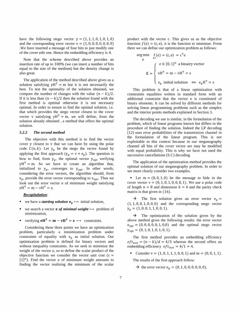
The scheme can be broadly summarized by the
following figure.
Figure5: Representation of the proposed steganographic
scheme.
5.2.3 Calculation of embedding efficiency
We will calculate the embedding efficiency of our
scheme for the case of a cover vector of size and a
message of bits. Thus and .
= [
]
By examining the columns of and those of
combining them two to two we have the following
equalities:
( )
( )
( )
( )
( )
( )
( )
The syndrome of size is equal to:
the zero vector ( ) with a probability of
no ( ) change of the cover vector;
a column of with a probability of
( different
vectors representing the column of on the possibles
of ( )) one ( ) change;
a sum of two distinct columns of with a
probability of
(7 vectors obtained by summation two to
two of the different columns of ) two ( ) changes.
The average number of changes made by the insertion
of the message is:
.
Thus the embedding efficiency is:
( )
.
For a relative payload
.
This value of the embedding efficiency is much greater
than ( ) and constitutes the largest possible
using a binary code with the same characteristics (
and ) for a constant profile.
5.2.4 Optimality condition of the proposed scheme
The proposed scheme is not suitable for messages of
size less than or equal to ( ), with the block
length of the polar code. Then the messages we want that
treatment with this scheme provides a minimum number of
changes must verify ( ) . To satisfy this
requirement we can adjust either the size of the message or
that of the vector cover. Because the message is given in
advance, it would be easier and wiser to choose the second
option which consists of choosing the cover vector so that
its size satisfies the criterion ( ) . This criterion
imposed is logic since for some columns of the
parity check matrix are related (they are identical because
we are in the binary case) which favors more changes. Note
that even messages of size m ≤ p can be inserted and
extracted at reception but the minimum number of changes
is no longer guaranteed.
To illustrate what we have said we choose
( ). If we take (i.e. ),
=[
]
with and .
The successive columns of H are 2 to 2 identical.
9
5.3 Steganographic scheme with wet paper
In the scheme we have defined, we considered the case
of a constant profile. We will show in this section that the
proposed scheme can be adapted to the case of wet paper.
In the case where the costs of embedding changes
(constant profile), the minimization of the distortion
amounts to minimize the number of modifications of the
cover vector by seeking the stego vector the closest to .
On the other hand if the are arbitrary in we have to
define the scheme for the minimization of the number of
changed positions by taking into account constraints of the
cost values . So we have to modify the pixels where the
changes are less perceptible (with the smallest values of ).
Fridrich and al. have identified three profile types for
steganographic schemes [6]: the constant profile ( ( ) ), the linear profile ( ( ) ) , and the square profile
( ( ) ). We will develop a technique of
steganography to minimize the embedding impact for a
given distortion.
Consider an arbitrary profile defined by 1
[13]. Our goal is to adapt the proposed scheme previously
to this general case of the distorted profiles. J. Fridrich and
al. [6] have proposed two methods to apply their scheme to
the case of wet papers. The first consists of locking a
certain number of positions (wet elements) of stego object
and change only the bits corresponding to the dry elements.
The success of this method depends, of course, on the
number of locked positions and the type of encoding used.
The value of should not exceed the dimension of the
code as defined also in [4] and [5]. Otherwise the search
of stego vector would provide no solution. The second
technique consists to lock the positions at which the
changes will be most visible. Fridrich and al. have also
shown that this method is well adapted in practice. If the
number of wet elements is greater than we allow
ourselves to change some2. To propose a method of
steganography with codes polar wet paper we will use the
latter approach which is more practical and suitable for our
scheme.
Since our scheme consists of two parts, the second
improves the first, it is thus necessary to see how each of
these two methods is applied to the case of wet papers.
Recall that the first method is closely related to the form
of the matrix parity check of the polar code and exploits the
1 The three types of profile are particulars cases of this consideration. 2 If we consider that the number of wet elements is equal to , we
can change of them.
steganography relation by locking some positions
of the cover vector. Consequently it is independent of the
type of the considered profile, and thus applies identically
to the case of constant profile. In this case if the solution
offered by this method corresponds to the optimal one it
will not be necessary to apply the second method.
Concerning the second method whose implementation
depends on the profile used, changes should be made to
define a scheme to wet paper steganography. The problem
is the same as in the case of constant profile (optimization
problem, specifically minimization), we will use the same
principle of linear programming to find our optimal
solution. The initial solution and the constraints have not
changed. What does change here is the objective function.
Indeed, in the case of constant profile, the goal was to
minimize the Hamming weight of error vector , while for
an arbitrary profile, the goal is to minimize the distortion
function ( ). Rewrite this relation and the functions of
insertion and extraction depending on the change vector :
( ) ∑
where | | and the modification
cost of the LSB of a pixel into .
( ) ( )
( )
( )
We can see that our objective function ( ) ⟨ ⟩, which must be written as a vector scalar product between
the cost vector of the linear program and the variable ,
appears well in the expression of ( ). Consequently the
cost elements of the vector are represented by changes the
costs of pixels during the insertion.
Let and we find the same form of
linear program. And the resolution can be done in the same
way that in the case of constant profile.
Note that we can also apply the first approach which
consists in fixing bits (wet elements) of the cover vector
by assigning values (large values in practice) and
values to dry elements. But the condition is
needed in this case.
6 EXPERIMENTAL RESULTS
To verify the efficiency of our scheme and the invisibility
of the hidden messages using this scheme, we have tested it
on different images in gray scale PGM format size (
10
) . The images are taken from the 3
database.
To make the message less detectable, we choose to
permute the pixels of the cover image before making the
insertion. Remember that we had a permutation matrix ,
square and of dimension a power of , that permutes the
rows of a given square matrix. And it happens that our
images are of size and is a power of . We
can use for the permutation. Thus the changes will be
spread over isolated pixels of the image making it less
detectable the secret message inserted and thus allowing a
more secure insertion. After insertion, it is necessary to find
the original order of pixels of the cover image. To achieve
this we still use the matrix . Since it is invertible and
equal to its own inverse, it suffices just to repeat the same
operation as in the permutation (matrix product of by the
matrix of the cover image). This choice of permutation is an
example among many others (we might use the matrix
for example) and may be secretly shared between the sender
and receiver.
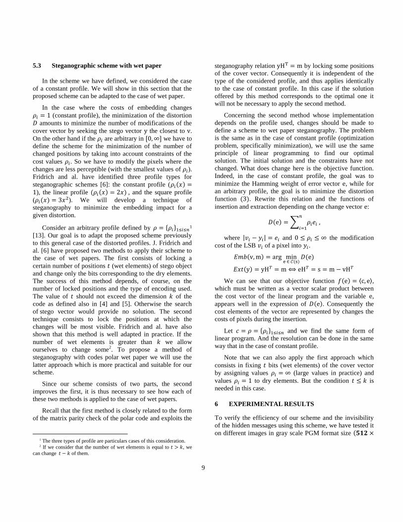
First we insert a message of size or in
an image (10.pgm) BOSS database. The first and most
simple evaluation to do concerns the visual
imperceptibility. The changes in the stego image are
invisible to the naked eye as shown in Figures 6. Hence the
first and main goal of steganography is achieved. If we are
confronted with a passive attacker we have clearly seen that
by comparing the cover and stego images on the one hand
and their histogram on the other hand, for an attacker to
"semi-active", the distinction between the two images is
almost impossible. Because there is a very small difference
between the histograms of the cover and stego images that
is very difficult to perceive. This difference is more
perceptible if the size of the message to be inserted
increases. The scheme is even more secure that the attacker
has only the stego image to see if it contains a secret
message or not. He should therefore use much more
sophisticated means to reach to detect the presence of secret
message.
3 (Break Our Stego-System): the competition for the pour les
attacks of the steganographic schemas.
Figure 6: The cover image 10.ppm and stego image 10_stego.png
and their histograms.
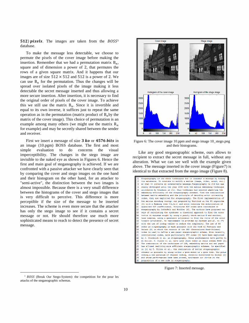
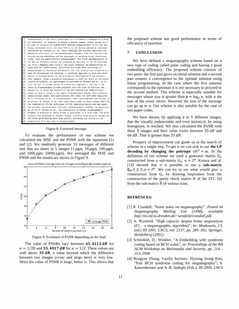
Like any good steganographic scheme, ours allows to
recipient to extract the secret message in full, without any
alteration. What we can see well with the example given
above. The message inserted in the cover image (Figure7) is
identical to that extracted from the stego image (Figure 8).
Figure 7: Inserted message.
11
Figure 8: Extracted message.
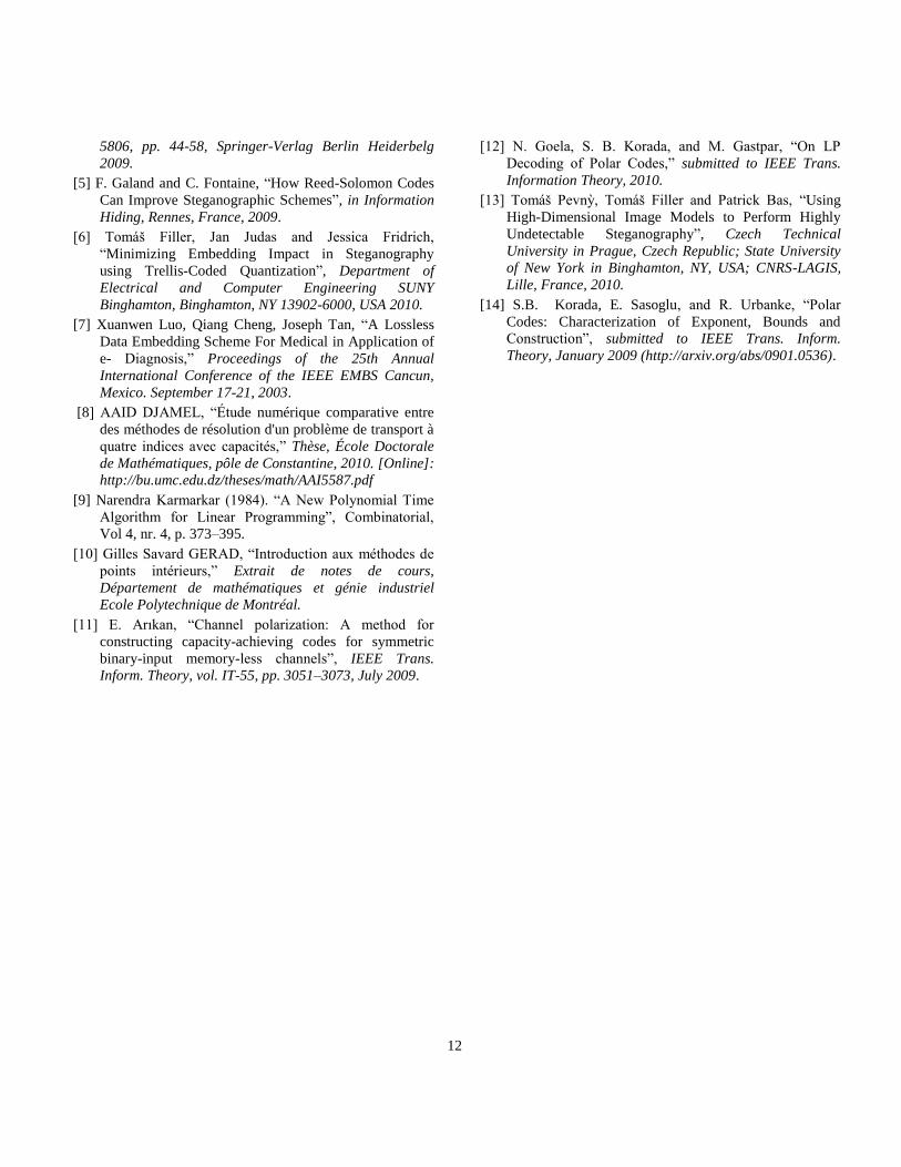
To evaluate the performance of our scheme we
calculated the MSE and the PSNR with the equations (1)
and (2). We randomly generate 10 messages of different
size that we insert in 5 images (1.pgm, 10.pgm, 100.pgm,
and 1000.pgm 10000.pgm). We averaged the MSE and
PNSR and the results are shown in Figure 9.
Figure 9: Evolution of PSNR depending on the load.
The value of PNSRs vary between for
and for . These values are
well above a value beyond which the difference
between two images (cover and stego here) is very low.
More the value of PSNR is large, better is. This shows that
the proposed scheme has good performance in terms of
efficiency of insertion.
7 CONCLUSION
We have defined a steganography scheme based on a
new type of coding called polar coding and having a good
embedding efficiency. The proposed scheme consists of
two parts: the first part gives an initial solution and a second
part ensures a convergence to the optimal solution using
linear programming. In the case where the first solution
corresponds to the optimum it is not necessary to proceed to
the second method. This scheme is especially suitable for
messages whose size is greater than , with the
size of the cover vector. However the size of the message
can go up to . Our scheme is also suitable for the case of
wet paper codes.
We have shown, by applying it to different images,
that the visually undetectable and even statistical, by using
histograms, is reached. We also calculated the PSNR with
these images and their value varies between and
. That is greater than .
Prospect of improvement can guide us in the search of
scheme in a single step. To get it we can sink to use the LP
decoding by changing the polytope . In the
definition of our scheme we used a generator matrix
constructed from a sub-matrix , . Korara and al.
[14] showed that it is possible to use a sub-matrix
. We can try to see what would give a
construction from by drawing inspiration from the
construction of the parity check matrix of the STC [6]
from the sub-matrix ̂ of various sizes.
REFRENCES:
[1] R. Crandall, “Some notes on steganography”, Posted on
Steganography Mailing List (1998), available
http://os.inf.tu-dresden.de/~westfeld/crandall.pdf.
[2] A. Westfeld, “High capacity despite better steganalysis
(F5 – a steganographic algorithm)”, In: Moskowitz, I.S.
(ed.) IH 2001. LNCS, vol. 2137, pp. 289–302, Springer,
Heidelberg (2001).
[3] Schönfeld, D., Winkler, “A Embedding with syndrome
coding based on BCH codes”, in: Proceedings of the 8th
ACM Workshop on Multimedia and Security, pp. 214 –
223, 2006.
[4] Rongyue Zhang, Vasiliy Sachnev, Hyoung Joong Kim,
“Fast BCH syndrome coding for steganography”; S.
Katzenbeisser and A.-R. Sadeghi (Eds.), IH 2009, LNCS
12
5806, pp. 44-58, Springer-Verlag Berlin Heiderbelg
2009.
[5] F. Galand and C. Fontaine, “How Reed-Solomon Codes
Can Improve Steganographic Schemes”, in Information
Hiding, Rennes, France, 2009.
[6] Tomáš Filler, Jan Judas and Jessica Fridrich,
“Minimizing Embedding Impact in Steganography
using Trellis-Coded Quantization”, Department of
Electrical and Computer Engineering SUNY
Binghamton, Binghamton, NY 13902-6000, USA 2010.
[7] Xuanwen Luo, Qiang Cheng, Joseph Tan, “A Lossless
Data Embedding Scheme For Medical in Application of
e- Diagnosis,” Proceedings of the 25th Annual
International Conference of the IEEE EMBS Cancun,
Mexico. September 17-21, 2003.
[8] AAID DJAMEL, “Étude numérique comparative entre
des méthodes de résolution d'un problème de transport à
quatre indices avec capacités,” Thèse, École Doctorale
de Mathématiques, pôle de Constantine, 2010. [Online]:
http://bu.umc.edu.dz/theses/math/AAI5587.pdf
[9] Narendra Karmarkar (1984). “A New Polynomial Time
Algorithm for Linear Programming”, Combinatorial,
Vol 4, nr. 4, p. 373–395.
[10] Gilles Savard GERAD, “Introduction aux méthodes de
points intérieurs,” Extrait de notes de cours,
Département de mathématiques et génie industriel
Ecole Polytechnique de Montréal.
[11] E. Arıkan, “Channel polarization: A method for
constructing capacity-achieving codes for symmetric
binary-input memory-less channels”, IEEE Trans.
Inform. Theory, vol. IT-55, pp. 3051–3073, July 2009.
[12] N. Goela, S. B. Korada, and M. Gastpar, “On LP
Decoding of Polar Codes,” submitted to IEEE Trans.
Information Theory, 2010.
[13] Tomáš Pevnỳ, Tomáš Filler and Patrick Bas, “Using
High-Dimensional Image Models to Perform Highly
Undetectable Steganography”, Czech Technical
University in Prague, Czech Republic; State University
of New York in Binghamton, NY, USA; CNRS-LAGIS,
Lille, France, 2010.
[14] S.B. Korada, E. Sasoglu, and R. Urbanke, “Polar
Codes: Characterization of Exponent, Bounds and
Construction”, submitted to IEEE Trans. Inform.
Theory, January 2009 (http://arxiv.org/abs/0901.0536).


![IEEE TRANSACTIONS ON INFORMATION FORENSICS AND …€¦ · Steganography is perfect if the embedding function preserves the cover distribution [2]. This requires knowledge of the](https://static.cupdf.com/doc/110x72/5f6f806d7e4efa107869373a/ieee-transactions-on-information-forensics-and-steganography-is-perfect-if-the-embedding.jpg)