Theory of Computation
Todd Gaugler
December 14, 2011

2
Contents
1 Mathematical Background 51.1 Overview . . . . . . . . . . . . . . . . . . . . . . . . . . . . . . . . . . . . . . . . . . 51.2 Number System . . . . . . . . . . . . . . . . . . . . . . . . . . . . . . . . . . . . . . 51.3 Functions . . . . . . . . . . . . . . . . . . . . . . . . . . . . . . . . . . . . . . . . . 61.4 Relations . . . . . . . . . . . . . . . . . . . . . . . . . . . . . . . . . . . . . . . . . . 61.5 Recursive Definitions . . . . . . . . . . . . . . . . . . . . . . . . . . . . . . . . . . . 81.6 Mathematical Induction . . . . . . . . . . . . . . . . . . . . . . . . . . . . . . . . . 9
2 Languages and Context-Free Grammars 112.1 Languages . . . . . . . . . . . . . . . . . . . . . . . . . . . . . . . . . . . . . . . . . 112.2 Counting the Rational Numbers . . . . . . . . . . . . . . . . . . . . . . . . . . . . . 132.3 Grammars . . . . . . . . . . . . . . . . . . . . . . . . . . . . . . . . . . . . . . . . . 142.4 Regular Grammar . . . . . . . . . . . . . . . . . . . . . . . . . . . . . . . . . . . . . 15
3 Normal Forms and Finite Automata 173.1 Review of Grammars . . . . . . . . . . . . . . . . . . . . . . . . . . . . . . . . . . . 173.2 Normal Forms . . . . . . . . . . . . . . . . . . . . . . . . . . . . . . . . . . . . . . 183.3 Machines . . . . . . . . . . . . . . . . . . . . . . . . . . . . . . . . . . . . . . . . . . 20
3.3.1 An NFA λ . . . . . . . . . . . . . . . . . . . . . . . . . . . . . . . . . . . . . 22
4 Regular Languages 234.1 Computation . . . . . . . . . . . . . . . . . . . . . . . . . . . . . . . . . . . . . . . 244.2 The Extended Transition Function . . . . . . . . . . . . . . . . . . . . . . . . . . . 244.3 Algorithms . . . . . . . . . . . . . . . . . . . . . . . . . . . . . . . . . . . . . . . . . 26
4.3.1 Removing Non-Determinism . . . . . . . . . . . . . . . . . . . . . . . . . . . 264.3.2 State Minimization . . . . . . . . . . . . . . . . . . . . . . . . . . . . . . . . 264.3.3 Expression Graph . . . . . . . . . . . . . . . . . . . . . . . . . . . . . . . . . 26
4.4 The Relationship between a Regular Grammar and the Finite Automaton . . . . . . 264.4.1 Building an NFA corresponding to a Regular Grammar . . . . . . . . . . . . 274.4.2 Closure . . . . . . . . . . . . . . . . . . . . . . . . . . . . . . . . . . . . . . 27
4.5 Review for the First Exam . . . . . . . . . . . . . . . . . . . . . . . . . . . . . . . . 284.6 The Pumping Lemma . . . . . . . . . . . . . . . . . . . . . . . . . . . . . . . . . . . 28
5 Pushdown Automata and Context-Free Languages 315.1 Pushdown Automata . . . . . . . . . . . . . . . . . . . . . . . . . . . . . . . . . . . 315.2 Variations on the PDA Theme . . . . . . . . . . . . . . . . . . . . . . . . . . . . . . 345.3 Acceptance of Context-Free Languages . . . . . . . . . . . . . . . . . . . . . . . . . 36
3
CONTENTS CONTENTS
5.4 The Pumping Lemma for Context-Free Languages . . . . . . . . . . . . . . . . . . . 365.5 Closure Properties of Context- Free Languages . . . . . . . . . . . . . . . . . . . . . 37
6 Turing Machines 396.1 The Standard Turing Machine . . . . . . . . . . . . . . . . . . . . . . . . . . . . . . 396.2 Turing Machines as Language Acceptors . . . . . . . . . . . . . . . . . . . . . . . . 406.3 Alternative Acceptance Criteria . . . . . . . . . . . . . . . . . . . . . . . . . . . . . 416.4 Multitrack Machines . . . . . . . . . . . . . . . . . . . . . . . . . . . . . . . . . . . 426.5 Two-Way Tape Machines . . . . . . . . . . . . . . . . . . . . . . . . . . . . . . . . . 426.6 Multitape Machines . . . . . . . . . . . . . . . . . . . . . . . . . . . . . . . . . . . . 426.7 Nondeterministic Turing Machines . . . . . . . . . . . . . . . . . . . . . . . . . . . . 436.8 Turing Machines as Language Enumerators . . . . . . . . . . . . . . . . . . . . . . . 44
7 Turing Computable Functions 477.1 Computation of Functions . . . . . . . . . . . . . . . . . . . . . . . . . . . . . . . . 477.2 Numeric Computation . . . . . . . . . . . . . . . . . . . . . . . . . . . . . . . . . . 487.3 Sequential Operation of Turing Machines . . . . . . . . . . . . . . . . . . . . . . . . 497.4 Composition of Functions . . . . . . . . . . . . . . . . . . . . . . . . . . . . . . . . 50
8 The Chomsky Hierarchy 518.1 Unrestricted Grammars . . . . . . . . . . . . . . . . . . . . . . . . . . . . . . . . . . 518.2 Context- Sensitive Grammars . . . . . . . . . . . . . . . . . . . . . . . . . . . . . . 52
8.2.1 Linear-Bounded Automata . . . . . . . . . . . . . . . . . . . . . . . . . . . . 528.2.2 Chomsky Hierarchy . . . . . . . . . . . . . . . . . . . . . . . . . . . . . . . . 53
9 Decidability and Undecidability 559.1 Church-Turing Thesis . . . . . . . . . . . . . . . . . . . . . . . . . . . . . . . . . . . 559.2 Universal Machines . . . . . . . . . . . . . . . . . . . . . . . . . . . . . . . . . . . . 559.3 The Halting Problem for Turing Machines . . . . . . . . . . . . . . . . . . . . . . . 569.4 Problem Reduction and Undecidability . . . . . . . . . . . . . . . . . . . . . . . . . 569.5 Rice’s Theorem . . . . . . . . . . . . . . . . . . . . . . . . . . . . . . . . . . . . . . 56
10 µ-Recursive Functions 57
11 Time Complexity 59
12 P ,NP, and Cook’s Theorem 61
4
Chapter 1
Mathematical Background
1.1 Overview
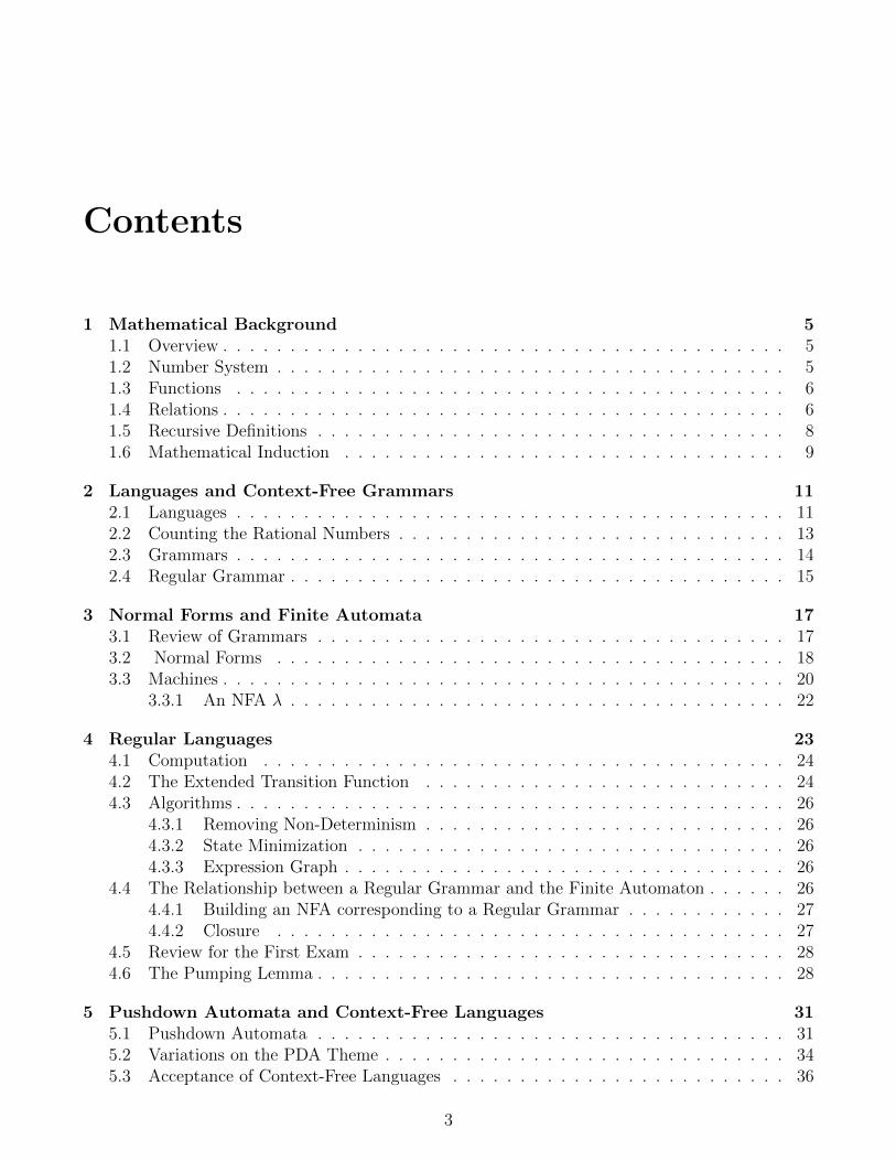
The Chaimsky Hierarchy of Languages (on page 339) is broken up into the following types:
Type Language Grammar Machine0 Recursively Enumerable Unrestricted Phrase Structure Turing Machine1 Contex-Sensitive Context-Sensitive Linear Bounded2 Context-Free Context-Free Pusmh-Down3 Regular Regular Finite Autmomaton.
1.2 Number System
The natural numbers, denoted N = {0, 1, 2, ...} will be important in this class, along with theintegers Z, the rational numbers Q, and the real numbers R. The irrational numbers, Q or R−Q.
Definition
A set is a collection of elements where no element appears more than once.
Some common examples of sets are the empty set, {} and singletons, which are sets that containexactly one element. The notion of a subset of some set S = {s1, s2, ....sn} is a new set R ={r1, r2, ...rn}, and R ⊆ S if for some j, ri = sj. A proper subset, denoted R ( S is a subset thatdoes not contain all the elements of S. The notion of a power set, denoted P(S) is the set of allsubsets of S. Given some set S with n elements, the cardinality (or number of elements in thatset) of P(S) is 2n.
5
1.3. FUNCTIONS CHAPTER 1. MATHEMATICAL BACKGROUND
Given two sets A,B we can talk about their union A ∪ B = {c, |c ∈ A orc ∈ B}. Similarly,intersection can be described as: A ∪ B = {c|c ∈ A and c ∈ B}. Union and intersection arecommutative. When taking the difference, A−B, we see that this operation is not commutative.These operations are known as binary operations.
Another important operation is the notion of the unary operation complementation. The com-plement of a set S can be written S ′, or Sc which considers the universe U in which S is contained,and S ′ = U − S.Example. Take the odd positive natural numbers. The compliment of the odd numbers dependson the universe in which you are placing these odd positive natural numbers. If we allowed theuniverse to be the integers Z, the compliment of this set would contain all odd and negative evenintegers.
Definition
Demorgans law: A ∪B = A ∩B and A ∩B = A ∪B
1.3 Functions
A function f : X → Y is unary, whereas the function f(x1, x2) is called a binary function. Thisnotion can be extended to the n case. A total function is a function which is defined for theentire domain. Many of the functions in this course will be of the form: f : N → N. However,looking at the function f(n) = n − 1, we see that this can’t possibly be defined for the entiredomain of N, since if you plug 0 into this function, the image under f of 0 is not contained inN. This such function is known as a partial function. However, we could redefine f such thatf(n) = n− 1 for all n ≥ 1, and if n = 0, f(n) = 0. This then becomes a total function.
Two other important properties of function are onto functions and one-to-one functions. If afunction is 1− 1, this means that f(a) = f(b)⇒ a = b. A function f is onto if its image is all ofthe set to which it is mapping. A function is bijective if it is both onto and one-to-one.
1.4 Relations
You can define x ∈ N as being in a relationship with y in the following way: [x, y]. Unlike afunction, an element x can be in relation with many other “outputs”. These relationships aresubsets of the Cartesian product N× N.
6
CHAPTER 1. MATHEMATICAL BACKGROUND 1.4. RELATIONS
Example. Let A = {2, 3} and let B = {3, 4, 5}. The Cartesian product is defined as follows:
A×B = {(a, b)|a ∈ A, b ∈ B}
The cardinality |A×B| = |A| × |B|.
Definition
Cardinality denotes the number of elements in some given set. A set has finite cardinality if thenumber of elements it contains is finite. A set has countably infinite cardinality if there exists abijection from that set to the natural numbers. A set has uncountable cardinality if it containsan infinite number elements, but there does not exist a bijection with that set and N.
Suppose we think of [0, 1) ( R. Any such number must be a decimal number, less than 1, that hassome sequence of numbers that corresponds to binary numbers. We will show that this intervalhas uncountable Cardinality through a proof by contradiction.
Proof. You can set up each number in this interval as:
r0 = 0.ba1ba1ba3 ....
r1 = 0.bb1bb1bb3 ....
r2 = 0.bc1bc1bc3 ....
r3 = 0.bd1bd1bd3 ....
And then you represent the new number:
rnew = bca1bcb2bcc3 ...
Which can be shown to not have been in our original list. 1
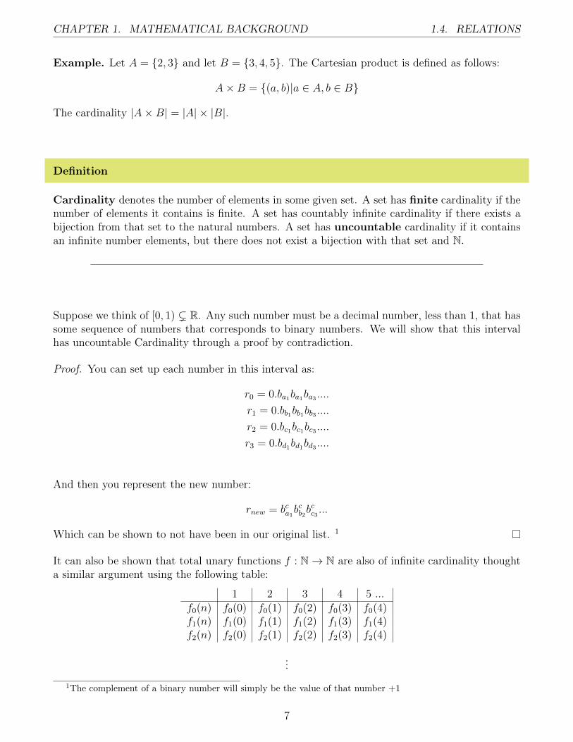
It can also be shown that total unary functions f : N→ N are also of infinite cardinality thoughta similar argument using the following table:
1 2 3 4 5 ...f0(n) f0(0) f0(1) f0(2) f0(3) f0(4)f1(n) f1(0) f1(1) f1(2) f1(3) f1(4)f2(n) f2(0) f2(1) f2(2) f2(3) f2(4)
...
1The complement of a binary number will simply be the value of that number +1
7
1.5. RECURSIVE DEFINITIONS CHAPTER 1. MATHEMATICAL BACKGROUND
It can also be shown that P(N) is of uncountable cardinality. The proof of this is in our book.
Another important notion for this class is the notion of a partition. A set S can be partitionedinto subsets A1, A2, ...An such that S = A1∪A2∪A3...∪An and that Ai∩Aj = ∅ if i 6= j. The lastproperty states that Ai, Aj are disjoint if i 6= j. This brings us back to the idea of an equivalencerelation.
Definition
An equivalence relation is a relation (I’ll say that a is related to b by writing a ? b) that satisfiesthe following:
1. a ? a
2. a ? b⇒ b ? a
3. a ? b, b ? c⇒ a ? c.
Some examples of an equivalence relation include:
1. Connectedness in a graph
2. Equivalence of vectors
3. Isomorphisms of groups, rings, etc.
The Barber’s Paradox: “There is a barber that shaves everyone that cannot shave themselves.So, does he shave himself?”
1.5 Recursive Definitions
For a recursive definition, we need the following:
1. A basis
2. A recursive step
3. A closure- if we can reach a result by starting with the basis and a finite number of applica-tions of the recursive step.
Example. Suppose you have m+ n, the addition of two numbers. So first, we define m+ 0 = m.Now, we define our recursive definition as m+ S(n) = S(m+ n). Think of it in this way:
m+ 0 = m
m+ 1 = S(m+ 0)
m+ 2 = S(m+ 1)
...
8
CHAPTER 1. MATHEMATICAL BACKGROUND 1.6. MATHEMATICAL INDUCTION
Which effectively defines addition, where S(n) is the “successor” of n.Example. Using the equivalence relation “less than”, we can first say that [0, 1], and that if [m,n],then [m,S(n)]. Similarly, [S(m), S(n)] is in the relation. This is an example of another recursivedefinition.
1.6 Mathematical Induction
Looking at the sum 1+2+3+4....+n we can prove inductively that this sum equals (n)(n+1)2
.
Proof. Our base case when n = 0 holds true for this formula, as does when n = 1. To proceed, wenow look at the inductive hypothesis, which says we will assume that indeed this formula works,and that we now need to prove that this works for the n+ 1th case. To show this, add 1 to n, plugit into the formula:
(n+ 1)(n+ 2)
2=
(n2 + 3n+ 2)
2=n(n+ 1) + 2n+ 2
2=
(n)(n+ 1)
2+ (n+ 1)
which tells us that the n+ 1th case holds.
We can show using strong induction that given a tree, |v| = |E|+ 2.
Proof. Given some tree, you can break it up into two separate pieces by separating it into twopieces via one edge. Then by the strong inductive hypothesis,
|v1| = |E1|+ 1, |v2| = |E2|+ 1
and we know that
|V | = |v1|+ |v2| = (|E1|+ 1) + (|E2|+ 1) + 1 = |E|+ 1
Where |E|+ 1 = |E1|+ |E2|+ 1
9
1.6. MATHEMATICAL INDUCTION CHAPTER 1. MATHEMATICAL BACKGROUND
10
Chapter 2
Languages and Context-FreeGrammars
2.1 Languages
Definition
There exists a set that we call the Alphabet Σ = {a, b, c} and, λ =denotes “the empty string”.
And we have the following identity for the element λ:
a = λa = aλ
And there exists the notion of an operation called concatenation, which is the notion we alllearned in CS111. This operation is NOT commutative. In other words, ab 6= ba. However,concatenation is associative- notice that the following are equivalent:
a(bc) = (ab)c
Where the ‘(‘ indicate the operation of concatenation. We can also talk about things like sub-strings and prefixes, which are fairly self-evident. Another operator to think about is the re-versal operator, which does the following:
aR = a, wordR = drow, (uv)R = vRuR
The last equality can be shown by mathematical induction:
11
2.1. LANGUAGES CHAPTER 2. LANGUAGES AND CONTEXT-FREE GRAMMARS
Proof.
the base case, |v| = 0(v = λ)
(uλ)R = uR = λuR = λRuR
now the case in which |v| = 1 :
(ua)R = a(uR) = aRuR
using the inductive hypothesis, we assume (uv)R = vRuR for |v| = n
we need to prove that (uw)R = wRuR for |w| = n+ 1,which we can represent as:
(uva)R = a(uv)R = avRuR = aRuRvR
and this is the same as:
(va)RuR = wRuR and |va| = |w| = n+ 1
Definition
If we write a∗, this denotes the set that includes {λ, a, an}. This operation is called the KleeneStar.Example. Given a word w,
w∗ = {λ,w,ww,www, ...}
We also talk about the union in the context of words. We can say:
u ∪ v = “either the word ‘u’, or the word ‘v’ ”
Using union, we can also speak about examples like u∪v∪w... We can put these operations in thecontext of a Regular Expression, which includes λ, a ∈ Σ, concatenation, Kleene Star (∗), and Union ∪.However, a regular expression does not have a concept of “intersection”, or “and”. We will allowa ”+” super script, where w+ denotes “one more copy of w”. This is allowed in a regular expres-sion because it is just a combination of two operations already existent in a regular expression;a+ = aa∗.
Definition
A Language L is the set of words over some alphabet Σ. A language can be empty, can be infinite,and can have one word.
12
CHAPTER 2. LANGUAGES AND CONTEXT-FREE GRAMMARS2.2. COUNTING THE RATIONAL NUMBERS
Example. one example of an infinite language can be the constructed by allows Σ = {a, b, c}.Our language L then consists of all 1, 2, 3, 4.... letter words, and this generates an infinite numberof words even though the length of the words has to remain finite. This is denoted Σ∗.
We can also talk about the set of all languages of Σ (this is a good multiple choice question).Example. The set of all languages over some alphabet Σ is like the power set P of our alphabetΣ∗, and is denoted P(Σ∗). Now while the cardinality of the |P (S)| = 2|S| when |S| is finite, notingthat Σ∗ is infinite, this won’t help us here. However, similar to the argument that the power setof the natural numbers was uncountable, we can use a similar diagonalization argument to showthat |P (S)| is uncountable.
To review, the following are used to denote certain operations:
L1 ∪ L2 unionL1L2 concatenationL∗ Kleene Starλ ∅
2.2 Counting the Rational Numbers
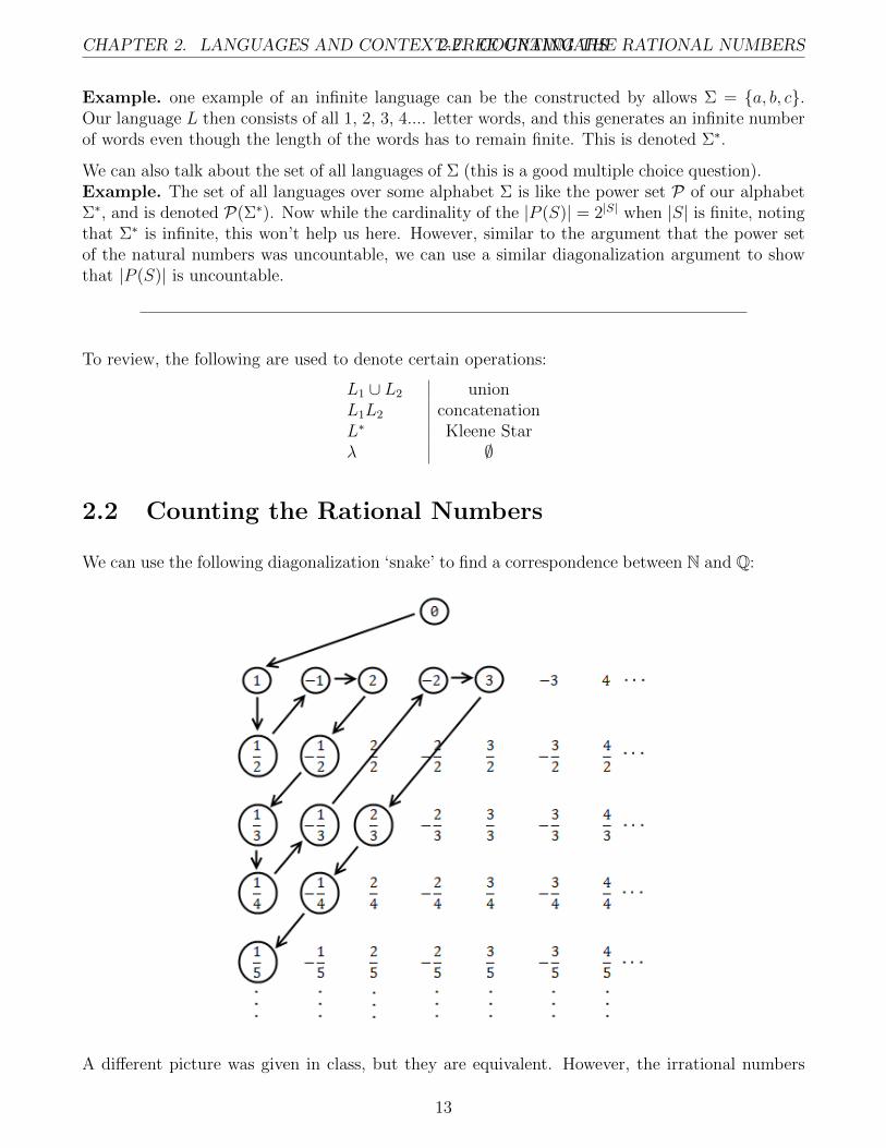
We can use the following diagonalization ‘snake’ to find a correspondence between N and Q:
A different picture was given in class, but they are equivalent. However, the irrational numbers
13
2.3. GRAMMARS CHAPTER 2. LANGUAGES AND CONTEXT-FREE GRAMMARS
R−Q are not countable, and no such diagonalization argument can be shown for them.
2.3 Grammars
Think about the way people talk- there exists some structure in which we all communicate. InEnglish, we use < nouns > and < verbs > and have rules to determine what is a ‘noun’ or a‘verb’. We are using the rules of grammar and applying them. This is very similar to the way inwhich Compilers view Code.
Definition
A Grammar has four components:
1. Variables
2. an alphabet
3. production rules
4. start symbols
This can be written as (V,Σ, P, S). Variables are usual capital letters, i.e. V = {A,B,C, ..}.Theseare also known as non-terminal letters, as opposed to the alphabet, which are terminal symbols.Using the special symbol S ∈ V , we apply a sequence of production rules to S, and this willeventually produce a word, ∈ Σ∗. A production rule for a context-free grammar is the following:V → (V ∪Σ)∗, where you take a Variable then change them to a sequence of variables and elementsin the alphabet.Example.
A→ aA, B → bCaB C → λ D → b
Let’s consider the case in which we have Σ = {a, b}, S, and P : {S → aSa, S → bSb, S → λ},V = {S}. And since S → aSa,→ aa We know that S
∗⇒ aa. Notice that this generates
palindromes over {a, b}, where these palindromes are of even length. For example,
S → aSa→ aaSaa→ aaaSaaa→ ....→ aaaaaa...︸ ︷︷ ︸evenlength
This can be remedied by saying P : S → {aSa, bSb, λ, a, b, }, of you could allow P to map S tosome other variables that map strictly to either a or b. From now on, we will use a vertical bar |to denote ‘or’ in the map P .
Now suppose you want to generate words of the form L = {ambn|n, n ≥ 0} . How would you dothis?
P : S → {AB|λ}, P : A→ {aA|λ}, P : B → {bB|λ}
14
CHAPTER 2. LANGUAGES AND CONTEXT-FREE GRAMMARS2.4. REGULAR GRAMMAR
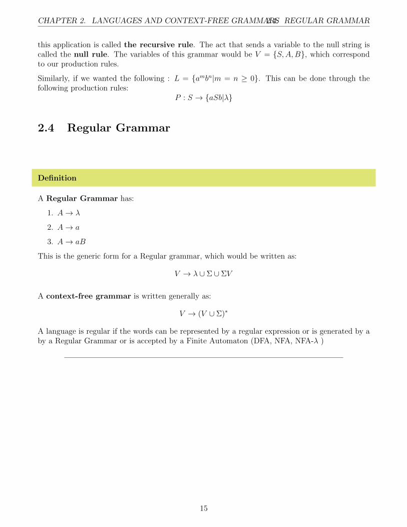
this application is called the recursive rule. The act that sends a variable to the null string iscalled the null rule. The variables of this grammar would be V = {S,A,B}, which correspondto our production rules.
Similarly, if we wanted the following : L = {ambn|m = n ≥ 0}. This can be done through thefollowing production rules:
P : S → {aSb|λ}
2.4 Regular Grammar
Definition
A Regular Grammar has:
1. A→ λ
2. A→ a
3. A→ aB
This is the generic form for a Regular grammar, which would be written as:
V → λ ∪ Σ ∪ ΣV
A context-free grammar is written generally as:
V → (V ∪ Σ)∗
A language is regular if the words can be represented by a regular expression or is generated by aby a Regular Grammar or is accepted by a Finite Automaton (DFA, NFA, NFA-λ )
15
2.4. REGULAR GRAMMARCHAPTER 2. LANGUAGES AND CONTEXT-FREE GRAMMARS
16
Chapter 3
Normal Forms and Finite Automata
The following are the notes that we took on the 13th of September.
3.1 Review of Grammars
Recall that a grammar is defined as follows:
G = (V,E, P,Σ)
Where:
1. V denotes the variables
2. Σ represents the alphabet
3. P represents the production
4. S represents the designated ‘start symbol’
If we have a Context-Free Grammar, we have the general form:
V → (V ∪ Σ)∗
Where a Regular grammar looks like the following:
V → λ ∪ Σ ∪ ΣV
This has to do with what i called the verification of grammars. We can talk about the languageof the grammar, L(G). Take the following example.Example. P : S → aSa|bSb|λ could be our production rule, which means our language wouldlook like even length palindromes over {a, b}. More formally, we are claiming that L(G) = evenlength palindromes over {a, b}. To prove as such, we need to show that everything produced underthis rule gives us such a word. This is fairly easy to see. Another way to do this would be to showthat every such palindrome would be generated through this production.Remark. A sentence is in sentential form when it is still on its way to being fully produced; it hasvariables left in it.
17
3.2. NORMAL FORMS CHAPTER 3. NORMAL FORMS AND FINITE AUTOMATA
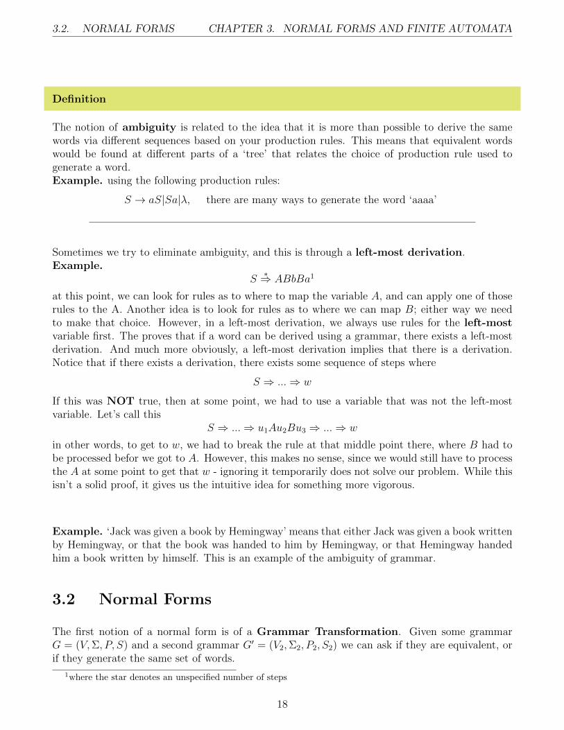
Definition
The notion of ambiguity is related to the idea that it is more than possible to derive the samewords via different sequences based on your production rules. This means that equivalent wordswould be found at different parts of a ‘tree’ that relates the choice of production rule used togenerate a word.Example. using the following production rules:
S → aS|Sa|λ, there are many ways to generate the word ‘aaaa’
Sometimes we try to eliminate ambiguity, and this is through a left-most derivation.Example.
S∗⇒ ABbBa1
at this point, we can look for rules as to where to map the variable A, and can apply one of thoserules to the A. Another idea is to look for rules as to where we can map B; either way we needto make that choice. However, in a left-most derivation, we always use rules for the left-mostvariable first. The proves that if a word can be derived using a grammar, there exists a left-mostderivation. And much more obviously, a left-most derivation implies that there is a derivation.Notice that if there exists a derivation, there exists some sequence of steps where
S ⇒ ...⇒ w
If this was NOT true, then at some point, we had to use a variable that was not the left-mostvariable. Let’s call this
S ⇒ ...⇒ u1Au2Bu3 ⇒ ...⇒ w
in other words, to get to w, we had to break the rule at that middle point there, where B had tobe processed befor we got to A. However, this makes no sense, since we would still have to processthe A at some point to get that w - ignoring it temporarily does not solve our problem. While thisisn’t a solid proof, it gives us the intuitive idea for something more vigorous.
Example. ‘Jack was given a book by Hemingway’ means that either Jack was given a book writtenby Hemingway, or that the book was handed to him by Hemingway, or that Hemingway handedhim a book written by himself. This is an example of the ambiguity of grammar.
3.2 Normal Forms
The first notion of a normal form is of a Grammar Transformation. Given some grammarG = (V,Σ, P, S) and a second grammar G′ = (V2,Σ2, P2, S2) we can ask if they are equivalent, orif they generate the same set of words.
1where the star denotes an unspecified number of steps
18
CHAPTER 3. NORMAL FORMS AND FINITE AUTOMATA 3.2. NORMAL FORMS
We need two things to establish L(G) = L(G′):
1. Every word in G can be generated by G′
2. Every word in G′ can be generated by G
Noticing immediately that the alphabets are the backbone of the words generated, it seems naturalto claim that the languages must have the same alphabets. However, this is not true- on occasion,some languages do not display certain letters (perhaps some languages do not have productionrules that allow certain letters to appear). For example, L = {} is one such example. However, itis true that when letters appear in one language, they must also appear in the other. Grammartransformation is the process under which we take a grammar and modify it by adding/changingvariables and production rules to transform it so that we get a grammar in a form we like, andretain the same language.
The first undesirable property of a grammar are called λ−rules. If λ is included in the language,then we must have some sort of λ rule to get λ. Thus, we need the rule S → λ. This does notmean that we can also have A → λ, since S is our start- symbol. How can we remove λ-rules?What you can do is replace all variables B → λ, you can work backwards and remove all λs. Forexample, suppose we had
S → aA|aBa|b|λ B → λ|bB A→ Aa|λ
we could switch this to the following:
S → aA|aB|b|λ|a B → bB|b A→ Aa|a
this is one method to remove λ-rules. Another undesirable property of grammars is called a chain rule.This looks like the following:
A→ B B → C
we end up combining these two to the following:
A→ C B → C, A→ B
we also have things called useless symbols
Definition
The Chaomsky Normal Form is an example of a normal form where all his rules obey thefollowing forms:
S → λ if there exists a λ rule
we could have
A→ a
and we could have
A→ BC
19
3.3. MACHINES CHAPTER 3. NORMAL FORMS AND FINITE AUTOMATA
the only catch is that B,C ∈ {V −{S}}, which says that these variables should not be S. This isbecause we want a non-recursive start symbol. One way of getting rid of a start symbol S wouldbe to define a new start symbol
S ′ → S
and that way, anything else that would be illegal for the start symbol would be legal, since it isn’ta start symbol anymore.
We will show that given something in Chomsky normal form and using the CYK algorithm, wecan generate a machine.
There exists another type of normal form, called the Greibach Normal Form, which includesthe following:
S → λ, A→ a, A→ aA1A2A3...An
one last undesirable feature is the eliminating of direct left recursion, which gives us somethingalong the lines of
A→ B [more variables]
we would like to move forward to our final product, not to more variables. Notice that Greibachnormal form avoids this by requiring that when adding more variables, at least one letter must beincluded.
3.3 Machines
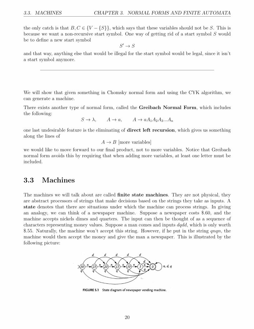
The machines we will talk about are called finite state machines. They are not physical, theyare abstract processors of strings that make decisions based on the strings they take as inputs. Astate denotes that there are situations under which the machine can process strings. In givingan analogy, we can think of a newspaper machine. Suppose a newspaper costs $.60, and themachine accepts nickels dimes and quarters. The input can then be thought of as a sequence ofcharacters representing money values. Suppose a man comes and inputs dqdd, which is only worth$.55. Naturally, the machine won’t accept this string. However, if he put in the string qnqn, themachine would then accept the money and give the man a newspaper. This is illustrated by thefollowing picture:
20
CHAPTER 3. NORMAL FORMS AND FINITE AUTOMATA 3.3. MACHINES
Where the machine has some ‘start state’, in which it expects $.60, and an accepting, or final state,where it has recieved the money it needs and need nothing else.
The finite state machine we’ll talk about are deterministic finite automatons (DEA)s, and aredefined as follows:
M = (Q,Σ, δ, q0, F )
1. Q stands for the set of states.
2. Σ is the alphabet.
3. δ is the transition function
4. q0 is the start state, which ∈ Q.
5. F is the set of final state(s), F ⊆ Q.
We know that L(M) : ∅ and L(M) : Σ∗. A transition function does the following:
δ : Q× Σ→ Q
this function is a total function. It takes in some input, looks at some input and the current state,and determines which state to go to next.
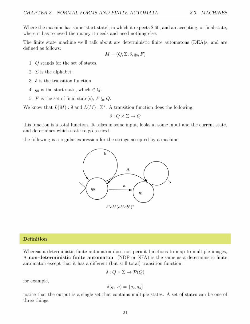
the following is a regular expression for the strings accepted by a machine:
A
a
b
q0q1
b
b∗ab∗(ab∗ab∗)∗
Definition
Whereas a deterministic finite automaton does not permit functions to map to multiple images,A non-deterministic finite automaton (NDF or NFA) is the same as a deterministic finiteautomaton except that it has a different (but still total) transition function:
δ : Q× Σ→ P(Q)
for example,δ(q1, a) = {q2, q3}
notice that the output is a single set that contains multiple states. A set of states can be one ofthree things:
21
3.3. MACHINES CHAPTER 3. NORMAL FORMS AND FINITE AUTOMATA
1. Empty ∅
2. A singleton {qi}
3. Multiple elements {q1, q2, ...qn}
So, a valid function for a non-deterministic finite automaton could be the following
δ(q1, b) = {}
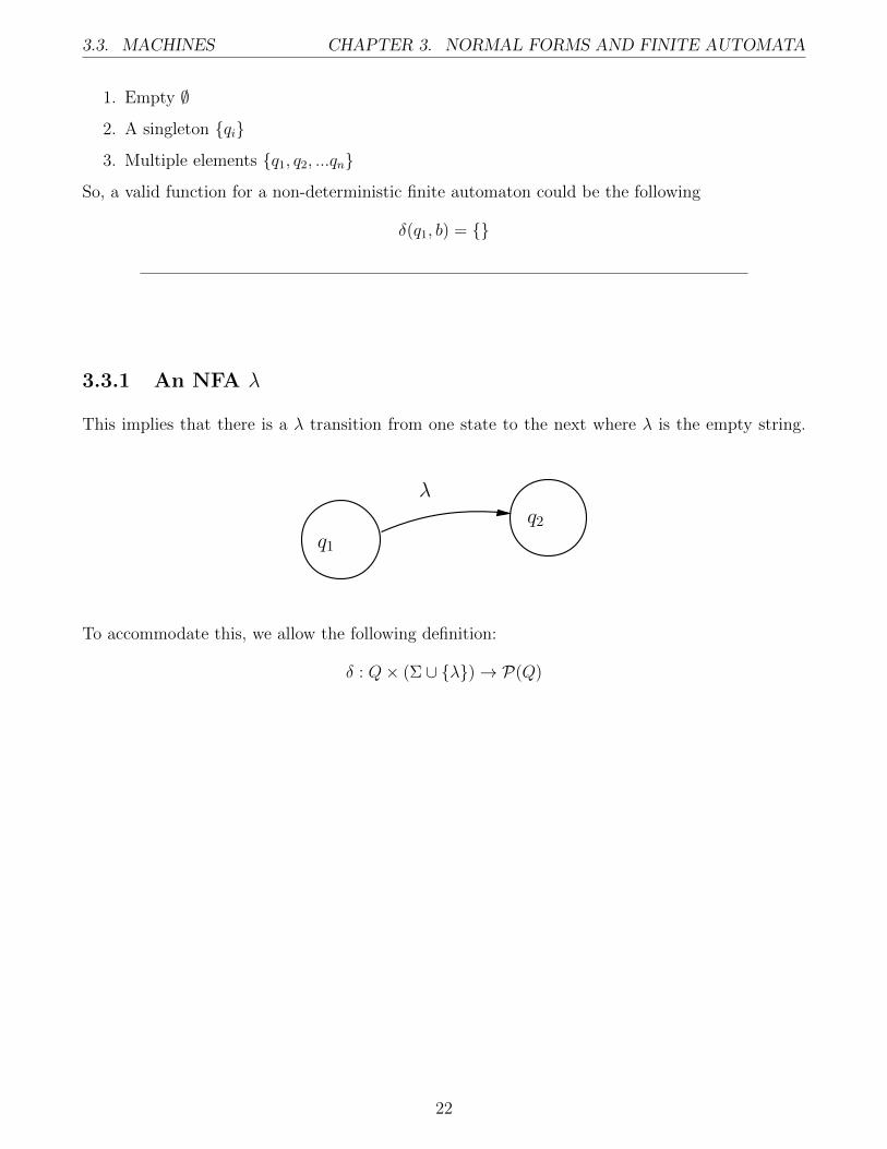
3.3.1 An NFA λ
This implies that there is a λ transition from one state to the next where λ is the empty string.
q1
q2
λ
To accommodate this, we allow the following definition:
δ : Q× (Σ ∪ {λ})→ P(Q)
22
Chapter 4
Regular Languages
Recall that a DFA is a machine denoted by M = (Q,Σ, δ, q0, F ), where the transition functionlooks like the following:
δ : Q× Σ→ Q
Also recall that an NFA is a machine denoted by M = Q,Σ, δ, q0, F ) where the transition functionlooks like:
δ : Q× Σ→ P(Q)
and in an NFA-λ, our transition function looks like:
δ : Q× (Σ ∪ {λ})→ P(Q)
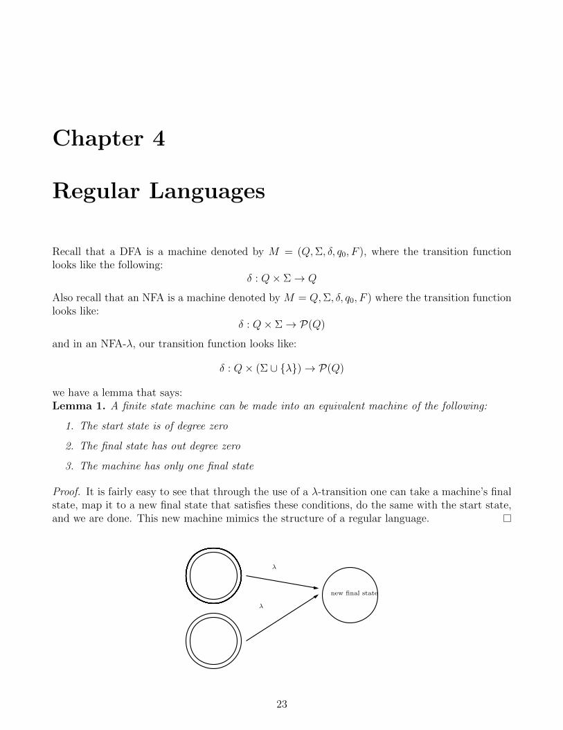
we have a lemma that says:Lemma 1. A finite state machine can be made into an equivalent machine of the following:
1. The start state is of degree zero
2. The final state has out degree zero
3. The machine has only one final state
Proof. It is fairly easy to see that through the use of a λ-transition one can take a machine’s finalstate, map it to a new final state that satisfies these conditions, do the same with the start state,and we are done. This new machine mimics the structure of a regular language.
λ
λ
new final state
23
4.1. COMPUTATION CHAPTER 4. REGULAR LANGUAGES
4.1 Computation
Computation is the process of starting a machine, doing computations, and determining whetheror not you are at a final start or not when finished. The process looks like the following:
[Qi, aw] 7→M [qj, w]
where the ‘w’ stands for the ‘word’, and this map has processed the ‘a’. Sometimes these blocksare called a machine configurations. A computation is the process of going from one machineconfiguration to the next. Just as we use a ‘*’ over the ⇒ to indicate that something can bederived in some amount of steps, we use the same symbol between machine configurations. Noticethat this is only possible if
δ(qi, a) = qi
4.2 The Extended Transition Function
For our purposes, an extended function is for a DFA. The difference between a extended transitionfunction and a transition function is that a transition function acts on one character. Meanwhile,the extended transition function:
δ(qi, w) = qi, δ : Q× Σ∗ → Q
takes entire words and maps them to states. Defining the extended transition function through arecursive definition, we use the following basis:
δ(qi, λ) = qi
and the basis
δ(qi, a) = δ(qi, a)
now inductively, we can say
δ(qi, wa) = δ(δ(q1, w), a), |w| = n, |wa| = n+ 1
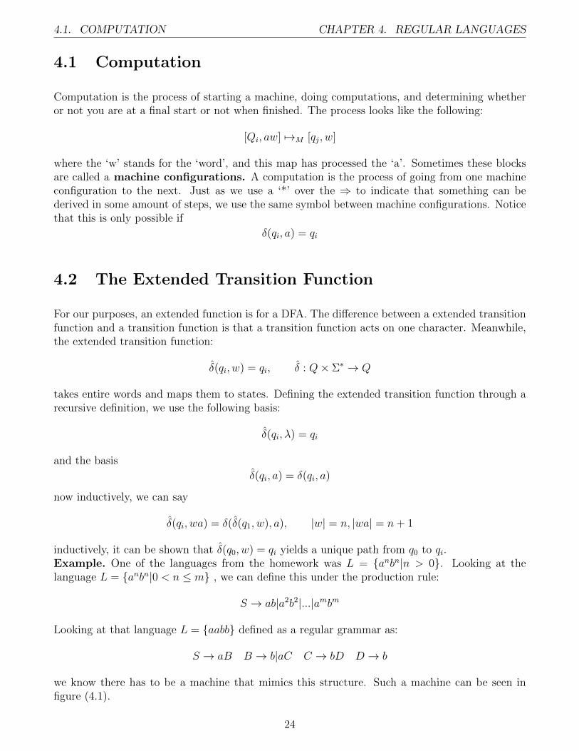
inductively, it can be shown that δ(q0, w) = qi yields a unique path from q0 to qi.Example. One of the languages from the homework was L = {anbn|n > 0}. Looking at thelanguage L = {anbn|0 < n ≤ m} , we can define this under the production rule:
S → ab|a2b2|...|ambm
Looking at that language L = {aabb} defined as a regular grammar as:
S → aB B → b|aC C → bD D → b
we know there has to be a machine that mimics this structure. Such a machine can be seen infigure (4.1).
24
CHAPTER 4. REGULAR LANGUAGES 4.2. THE EXTENDED TRANSITION FUNCTION
a a a
bbb
am
Figure 4.1: L = {anbn|0 < n ≤ m}
Definition
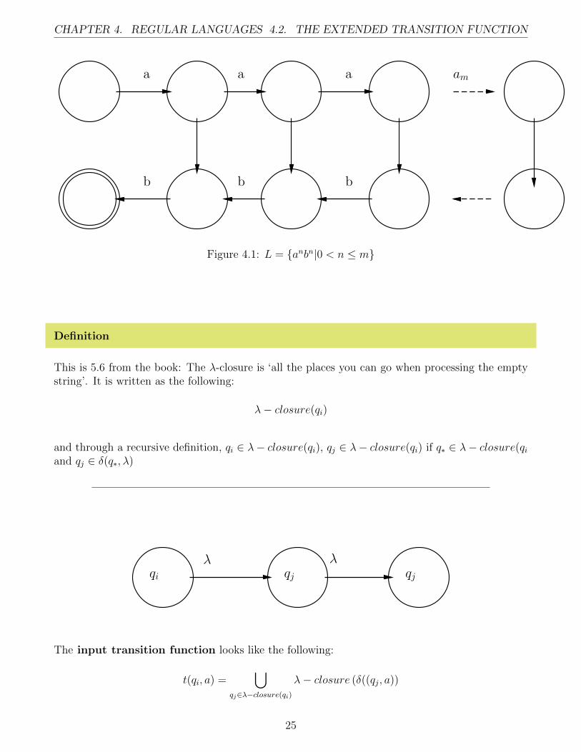
This is 5.6 from the book: The λ-closure is ‘all the places you can go when processing the emptystring’. It is written as the following:
λ− closure(qi)
and through a recursive definition, qi ∈ λ− closure(qi), qj ∈ λ− closure(qi) if q∗ ∈ λ− closure(qiand qj ∈ δ(q∗, λ)
λ λqi qj qj
The input transition function looks like the following:
t(qi, a) =⋃
qj∈λ−closure(qi)
λ− closure (δ((qj, a))
25
4.3. ALGORITHMS CHAPTER 4. REGULAR LANGUAGES
4.3 Algorithms
4.3.1 Removing Non-Determinism
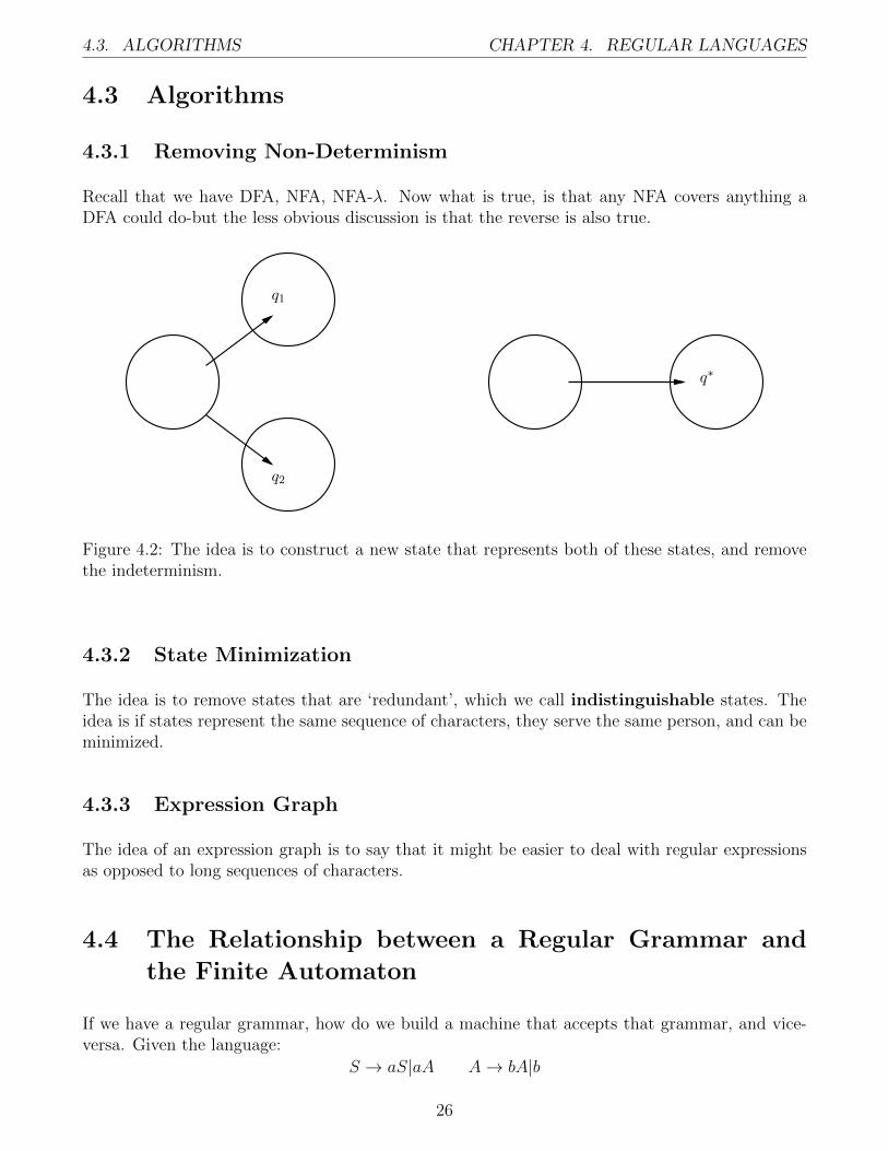
Recall that we have DFA, NFA, NFA-λ. Now what is true, is that any NFA covers anything aDFA could do-but the less obvious discussion is that the reverse is also true.
q1
q2
q∗
Figure 4.2: The idea is to construct a new state that represents both of these states, and removethe indeterminism.
4.3.2 State Minimization
The idea is to remove states that are ‘redundant’, which we call indistinguishable states. Theidea is if states represent the same sequence of characters, they serve the same person, and can beminimized.
4.3.3 Expression Graph
The idea of an expression graph is to say that it might be easier to deal with regular expressionsas opposed to long sequences of characters.
4.4 The Relationship between a Regular Grammar and
the Finite Automaton
If we have a regular grammar, how do we build a machine that accepts that grammar, and vice-versa. Given the language:
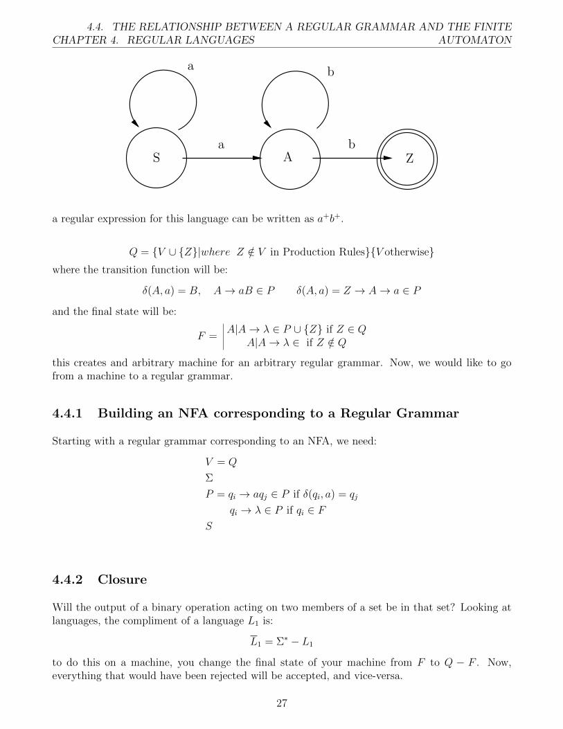
S → aS|aA A→ bA|b
26
CHAPTER 4. REGULAR LANGUAGES4.4. THE RELATIONSHIP BETWEEN A REGULAR GRAMMAR AND THE FINITE
AUTOMATON
S ZAa b
a b
a regular expression for this language can be written as a+b+.
Q = {V ∪ {Z}|where Z /∈ V in Production Rules}{V otherwise}where the transition function will be:
δ(A, a) = B, A→ aB ∈ P δ(A, a) = Z → A→ a ∈ P
and the final state will be:
F =A|A→ λ ∈ P ∪ {Z} if Z ∈ Q
A|A→ λ ∈ if Z /∈ Q
this creates and arbitrary machine for an arbitrary regular grammar. Now, we would like to gofrom a machine to a regular grammar.
4.4.1 Building an NFA corresponding to a Regular Grammar
Starting with a regular grammar corresponding to an NFA, we need:
V = Q
Σ
P = qi → aqj ∈ P if δ(qi, a) = qj
qi → λ ∈ P if qi ∈ FS
4.4.2 Closure
Will the output of a binary operation acting on two members of a set be in that set? Looking atlanguages, the compliment of a language L1 is:
L1 = Σ∗ − L1
to do this on a machine, you change the final state of your machine from F to Q − F . Now,everything that would have been rejected will be accepted, and vice-versa.
27
4.5. REVIEW FOR THE FIRST EXAM CHAPTER 4. REGULAR LANGUAGES
4.5 Review for the First Exam
Just as a trick, notice that a DFA is also a NFA and an NFA− λ, they are all equivalent.
We have said that L = {anbn|n ≥ 0} is non regular. Now suppose that we bound n above by n- isthis regular? It turns out that it is- having a finite selection gives us a regular language. We havealready seen what this looks like in terms of a Machine.
4.6 The Pumping Lemma
Let L be a language that is accepted by a DFA with K states. Let z be any string in L with
length(z) ≥ k
Then, z can be written as uvw with length
length(uv) ≤ k, length(v)
and uviw ∈ L for all i ≥ 0. It can be used to prove that languages are not regular. However, itcannot be used to prove that a language is regular.Example. Let L = {ai|i is prime}. We have K states, and consider some word an that will bebroken down into uvw, as our lemma says, then can be ‘pumped’. We’ll do the following:
uvi+1w
and consider the length of this word, which gives us:
length(uvi+1w) = |u|+|vi+1|+|w| = |u|+(n+1)|v|+|w| = |u|+|v|+n|v|+|w| = n+n|v| = n(1+|v|)
now what this means, as that the length of this string is n the length of that word v + 1. Weknow that this is a composite number, since it is the product of two numbers (neither of which is1, since |v| > 0). Thus, this language is not regular.Example. Let L = {am| m is a perfect square} Notice that the length of ak
2is clearly k2, which
is a perfect square. In this case the number of states will be K. According to the pumping lemma,
aK = uvw |v| > 0
as before, we consider
|uv2w| = |uvw|+ |v| = K2 + |v| ≤ K2 +K < K2 +K +K + 1 = (K + 1)2
but at the same time, we know:K2 < |uv2w| < (K + 1)2
thus, |uvw| can’t be a perfect square. This means that our assumption is incorrect- that ourlanguage is regular. Thus, this language is not regular.
The Pumping lemma is necessary for a language to be regular, but is not sufficient. The followingis section 6.7:
28
CHAPTER 4. REGULAR LANGUAGES 4.6. THE PUMPING LEMMA
Theorem 2. The Myhill-Necode Theorem: Given u, v ∈ Σ∗, where uw ∈ L whenever vw ∈ L,and uw /∈ L whenever vw /∈ L. We then call u and v indistinguishable- they basically behave inthe same way. They behave nicely with reflexive, symmetric, and transitive properties.Example. Consider {aibi|i ≥ 0} and the word aibj. Now looking at aibiaibj, this word does not be-have as something inside of the language-but, we are saying that ai and aj are not indistinguishable-since depending on what is put after them, sometimes you will have something in the languageand sometimes you won’t. I.e.,
aibi ∈ L ajbi /∈ L
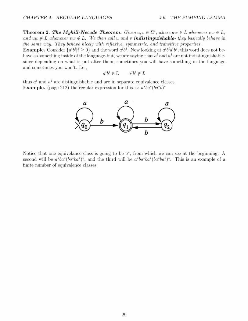
thus ai and aj are distinguishable and are in separate equivalence classes.Example. (page 212) the regular expression for this is: a∗ba∗(ba∗b)∗
Notice that one equivelance class is going to be a∗, from which we can see at the beginning. Asecond will be a∗ba∗(ba∗ba∗)∗, and the third will be a∗ba∗ba∗(ba∗ba∗)∗. This is an example of afinite number of equivalence classes.
29
4.6. THE PUMPING LEMMA CHAPTER 4. REGULAR LANGUAGES
30
Chapter 5
Pushdown Automata and Context-FreeLanguages
Recall that we decided that regular languages are generated by regular grammars, and acceptedby finite automata. However, also recall that there were certain limitations to what a finiteautomata could accept: For example, the language {aibi |i ≥ 0} could not have been accepted bya deterministic finite automaton because it had no ability to “remember” what amount of elementshad already been accepted. This is our motivation for things called Pushdown Automata
5.1 Pushdown Automata
For a machine to accept the language {aibi|i ≥ 0}, it needs to have the ability to record theprocessing of any finite number of a′s. The restriction of having finitely many states does notallow the automatons we discussed previously to do such a thing. Thus, we define a new typeof automaton that augments the state-input transitions of a finite automaton with the ability toutilize unlimited memory.
A pushdown stack, or simply a stack, is added to a finie automaton to construct a new machineknown as a pushdown automaton (PDA). stack operations affect only the top item of the stack:a pop removes the top element from the stack, and a push places and element on the top of thestack. Formally, we have the following definition:
Definition
A pushdown automaton is a sextuple:
(Q,Σ,Γ, δ, q0, F )
Where:
1. Q is a finite set of states
31
5.1. PUSHDOWN AUTOMATACHAPTER 5. PUSHDOWN AUTOMATA AND CONTEXT-FREE LANGUAGES
2. Σ is a finite set called the input alphabet
3. Γ is a finite set called the stack alphabet
4. q0 is the start state
5. F ⊆ Q is a set of final states,
6. δ is a transition function of the form:
δ : Q× (Σ ∪ {λ})× (Γ ∪ {λ})→ Q× (Γ ∪ {λ})
Notice that this tells us that a PDA has two alphabets, one from which the input strings are builtand a stack alphabet Γ whose elements are stored on top of the stack. The stack is representedas a string of stack elements, the elements on the top of the stack is the leftmost symbol in thestring. We use capital letters to represent Stack elements. The notation Aα represents a stackwith A as the top element, and an empty stack is denoted λ. The computation ofa PDA startswith the machine in state q0, the input on the tape, and the stack empty. Notice that we have thefollowing map for a transition function:
δ(qi, a, A)→ {[qj, B], [qk, C]}
which indicates that two transitions are possible when the automaton is in state qi, scanning an awith A on top of the stack. The transition:
[qj, B] ∈ Im(δ)
causes the machine to do all of the following:
1. Change the state from qi to qj
2. Process the symbol a
3. Remove A from the top of the stack
4. Push B onto the stack
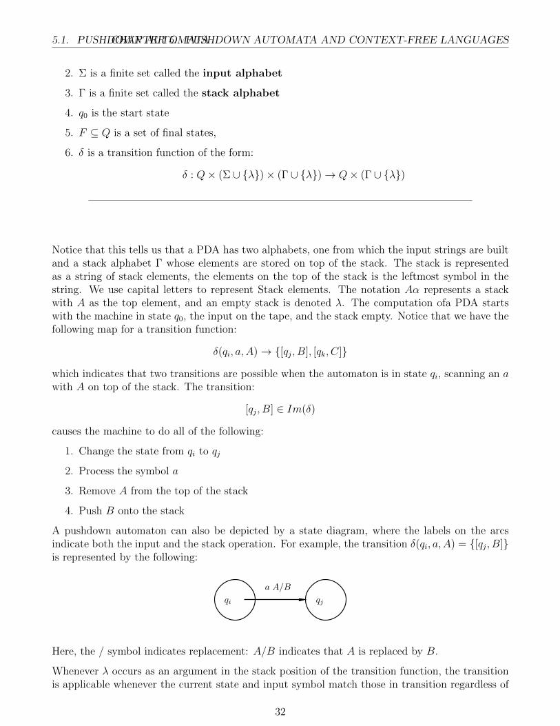
A pushdown automaton can also be depicted by a state diagram, where the labels on the arcsindicate both the input and the stack operation. For example, the transition δ(qi, a, A) = {[qj, B]}is represented by the following:
qi qj
a A/B
Here, the / symbol indicates replacement: A/B indicates that A is replaced by B.
Whenever λ occurs as an argument in the stack position of the transition function, the transitionis applicable whenever the current state and input symbol match those in transition regardless of
32
CHAPTER 5. PUSHDOWN AUTOMATA AND CONTEXT-FREE LANGUAGES5.1. PUSHDOWN AUTOMATA
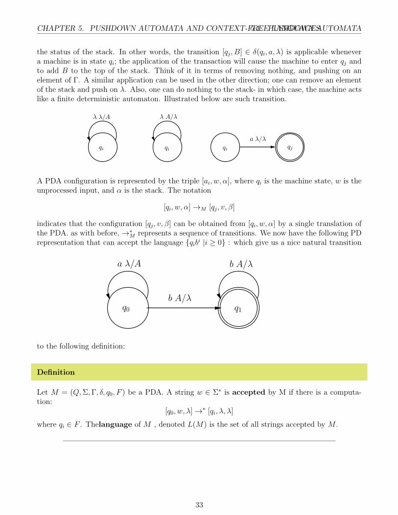
the status of the stack. In other words, the transition [qj, B] ∈ δ(qi, a, λ) is applicable whenevera machine is in state qi; the application of the transaction will cause the machine to enter qj andto add B to the top of the stack. Think of it in terms of removing nothing, and pushing on anelement of Γ. A similar application can be used in the other direction; one can remove an elementof the stack and push on λ. Also, one can do nothing to the stack- in which case, the machine actslike a finite deterministic automaton. Illustrated below are such transition.
λ A/λ
a λ/λ
λ λ/A
qi qi qi qj
A PDA configuration is represented by the triple [ai, w, α], where qi is the machine state, w is theunprocessed input, and α is the stack. The notation
[qi, w, α]→M [qj, v, β]
indicates that the configuration [qj, v, β] can be obtained from [qi, w, α] by a single translation ofthe PDA. as with before,→∗M represents a sequence of transitions. We now have the following PDrepresentation that can accept the language {qibi |i ≥ 0} : which give us a nice natural transition
a λ/A b A/λ
q1q0
b A/λ
to the following definition:
Definition
Let M = (Q,Σ,Γ, δ, q0, F ) be a PDA. A string w ∈ Σ∗ is accepted by M if there is a computa-tion:
[q0, w, λ]→∗ [qi, λ, λ]
where qi ∈ F . Thelanguage of M , denoted L(M) is the set of all strings accepted by M .
33
5.2. VARIATIONS ON THE PDA THEMECHAPTER 5. PUSHDOWN AUTOMATA AND CONTEXT-FREE LANGUAGES
Definition
A PDA is deterministic if there is at most one transition that is applicable for each combinationof state, input symbol, and stack top.
In previous chapters, we showed that deterministic and nondeterministic finite automata acceptedthe same family of languages. Nondeterminism was a useful design feature but did not increasethe ability of the machine to accept languages. This is not the case for pushdown automata. Forexample, there is no deterministic PDA that accepts the language L = {wwR |w ∈ {a, b}∗}.
5.2 Variations on the PDA Theme
Pushdown automata are often defined in a manner that differs from our traditional definition.There exist several altercations that preserve the set of accepted languages. Along with changingthe state, a transition in a PDA is accompanied by three actions: popping the stack, pushing astack element, and processing an input symbol. A PDA is called atomic if each transition causesonly one of these actions to occur. Transitions in an atomic PDA have the form:
1. [qj, λ] ∈ δ(qi, a, λ)
2. [qj, λ] ∈ δ(qi, λ, A)
3. [qj, A] ∈ δ(qi, λ, λ)
Clearly, every atomic PDA is a PDA in the sense of our definition Moreover, we have a method toconstruct an equivalent atomic PDA from an arbitrary PDA:Theorem 3. Let M be a PDA then there is an atomic PDA M ′ with L(M ′) = L(M).
Proof. This can be shown by taking all the non atomic transitions of M and replacing them bysequences of atomic transitions. For example, let [qj, B] ∈ δ(qi, a, A) be a transition of M . Theatomic equivalent requires two new states, p1, p2, and the transitions:
[p1, λ] ∈ δ(qi, q, λ)
δ(p1, λ, A) = {[p1, λ]}δ(p2, λ, λ) = {[qj, B]}
An extended transition is an operation on a PDA that pushes a string of elements rather thanjuts a single element, onto the stack. The transition [qj, BCD] ∈ δ(qi, a, A) pushes BCD onto thestack with B becoming the new stack top. A PDA containing extended transitions is called anextended PDA. The apparent generalization does not increase the set of languages accepted bypushdown automata. Each extended PDA can be converted into an equivalent PDA in the senseof our definition.
34
CHAPTER 5. PUSHDOWN AUTOMATA AND CONTEXT-FREE LANGUAGES5.2. VARIATIONS ON THE PDA THEME
To construct a PDA from an extended PDA, extended transitions are transformed into a sequenceof transitions each of which pushes a single stack element. To achieve the result of an extendedtransition that pushes k elements requires k − 1 additional states. We have the following theo-rem:Theorem 4. Let M be an extended PDA. Then there is a PDA M ′ such that L(M) = L(M ′).Example. We can construct a standard PDA, an atomic PDA, and an extended PDA to acceptthe language L = {aib2i | i ≥ 1}. As might be expected, the atomic PDA requires more transitionsand the extended PDA requires fewer transitions than the equivalent standard PDA.6
Definition
By a previous definition, an input string is accepted if there is a computation that processes theentire string and terminates in an accepting state with an empty stack. This type of acceptance isreferred to as acceptance by final state and empty stack. Defining acceptance in terms of thefinal state or in the configuration of the stack alone does not change the set of languages recognizedby pushdown automaton. A string w is accepted by final state if there exists a computation
[q0, w, λ]→∗m [qi, λ, α]
where qi is an accepting state and α ∈ Γ. That is, a computation that processes the input andterminates in an accepting state. The contents of the stack at termination are irrelevant withacceptance by final state. A language accepted by final state is denoted LF .
Lemma 5. Let L be a language accepted by a PDA M ′ = (Q ∪ {qf},Σ,Γ, δ′, q0, {qf}, F ) withacceptance defined by final state. Then there is a PDA that accepts L by final state and emptystack.
Proof. Intuitively, a computation in M ′ that accepts a string should be identical to one in Mexcept for the addition of transitions that empty the stack.
Lemma 6. Let L be a language accepted by PDA M = (Q,Σ,Γ, δ, q0) and with acceptance definedby empty stack- that is, there is a computation that take an input string and gets to a state whereinthe stack is empty, and there are no restrictions on the halting state. There is a PDA that acceptsL by final state and empty stack.
Combining these two lemmas give us the following theorem:Theorem 7. The following three conditions are equivalent:
1. The language L is accepted by some PDA.
2. There is a PDA M1 with LF (M1) = L.
3. There is a PDA M2 with LE(M2) = L.
35
5.3. ACCEPTANCE OF CONTEXT-FREE LANGUAGESCHAPTER 5. PUSHDOWN AUTOMATA AND CONTEXT-FREE LANGUAGES
5.3 Acceptance of Context-Free Languages
Theorem 8. Let L be a context-free language. There is then a PDA that accepts L.
Proof. First, we need to show that every context-free language is accepted by an extended PDA.This follows from taking a language in Greibach normal form, and then constructing a PDA thataccepts all words in that language. It then follows that we can construct a standard PDA thataccepts that context-free language.
Alternatively, we have the following theorem:Theorem 9. Let M be a PDA. Then there is a context-free grammar G with L(G) = L(M).
5.4 The Pumping Lemma for Context-Free Languages
The Pumping lemma for regular languages tells us that sufficiently long strings in a regular languagehave a substring that can be ‘pumped’ any number of times while still remaining in the language.There is an analogous lemma for context free languages.Theorem 10. Let L be a context-free language. There is a number k, depending on L, such thatany string z ∈ L with length(z) > k can be written as z = uvwxy where:
1. length(vwx) ≤ k
2. length(v) + length(x) > 0
3. uviwxiy ∈ L for i ≥ 0
The Proof will be omitted, but we have the following examples:Example. The language L = {aibici|i ≥ 0} is not context free. Assume the opposite. By thepumping lemma, the string z = akbkck can be decomposed into substrings uvwxy that satisfysome repetition properties. Consider the possibilities for the substrings v and x. If either of thesecontains moer than one type of terminal symbol, then uv2wx2y contains a b preceeding an a or ac preceding a b. In either case, the string is not in L.
By the previous observation, v, x must be substrings of one of ak, bk, or ck. Since at most one ofthe strings v, x is null, uv2wx2y increases the number of at least one, maybe two, but not all threetypes of terminal symbols. This implies that uv2wx2y /∈ L. Thus, L is not context-free, since itdoes not satisfy the pumping lemma.Example. The language L = {aibjaibj | i, j ≥ 0} is not context- free. Let k be the numberspecified by the pumping lemma and let z = akbkakbk. Assume there is a decomposition uvwxy ofz that satisfies the pumping lemma. By the first conditionn of the lemma, length(vwx) can be atmost k. This implies that vwx is a string containing only one type of terminal or the concatenationof two such strings. That is,
1. vwx ∈ a∗ or vwx ∈ b∗
2. vwx ∈ a∗b∗ or vwx ∈ b∗a∗
By an argument similar to the one in the previous example, the substrings v, x must only containone type of terminal. Pumping v and x increases the number of a′s or b′s in only one of the
36
CHAPTER 5. PUSHDOWN AUTOMATA AND CONTEXT-FREE LANGUAGES5.5. CLOSURE PROPERTIES OF CONTEXT- FREE LANGUAGES
substrings in z. Since there is no decomposition of z satisfying the conditions of the pumpinglemma, we conclude that L is not context free.Example. The language L = {w ∈ a∗ | length(w) is prime} is not context free. Assume that L iscontext free, and let n be a prime greater than k. The string an must have a decomposition uvwxythat satisfies the conditions of the pumping lemma. Let m = length(u) + length(w) + length(v).The length of any string uviwxiy is m + i(n − m). In particular, length(wvn+1wxn+1y) = m +(n+ 1)(n−m) = n(n−m+ 1). Both of the terms in the preceding product are natural numbersgreater than one, and as a result, this string is not in L. Thus, L is not context-free.
5.5 Closure Properties of Context- Free Languages
Operations that preserve context-free languages provide another tool for proving that languagesare context free.Theorem 11. The Family of context-free languages is closed under the operations of union, con-catenation, and Kleene star.Theorem 12. The set of context-free languages is not closed under intersection or complementa-tion.Theorem 13. Let R be a regular language and L be a context-free language. Then, R ∩ L is acontext- free language.Example. The langauge L = {ww | w ∈ {a, b}∗} is not context-free but L is. First we show thatL is not context-free using a proof by contradiction. Assume that L is context free. Then, by oneof our above theorems,
L⋂
a∗b∗a∗b∗ = {aibjaibj | i, j ≥ 0}
is context free, and we know that it isn’t - contradicting our assumption. To show that L is contextfree, we construct two context-free grammars G1, G2 such that L(G1)∪L(G2) = L. What one cando is to let G1 generate all even-length strings in {a, b}∗ and G2 generate all odd length strings in{a, b}∗. Both of these can be shown to be context free, in which case we are done.
37
5.5. CLOSURE PROPERTIES OF CONTEXT- FREE LANGUAGESCHAPTER 5. PUSHDOWN AUTOMATA AND CONTEXT-FREE LANGUAGES
38
Chapter 6
Turing Machines
6.1 The Standard Turing Machine
The Turing machine is a finite-state machine in which a transition prints a symbol on a ‘tape’.The tape head may move in either direction, allowing the machine to read and manipulate theinput as many times as desired.
Definition
A Turing Machine is a quintuple M = (Q,Σ,Γ, δ, q0) where Q is a finite set of states, Γ is afinite set called the tape alphabet, Γ contains a special symbol B that represents a blank, Σ is asubset of Γ− {B} called the input alphabet, δ is a partial function from
δ : Q× Γ→ Q× Γ× {L,R}
called the transition function, and q0 is a distinguished state called that start state.
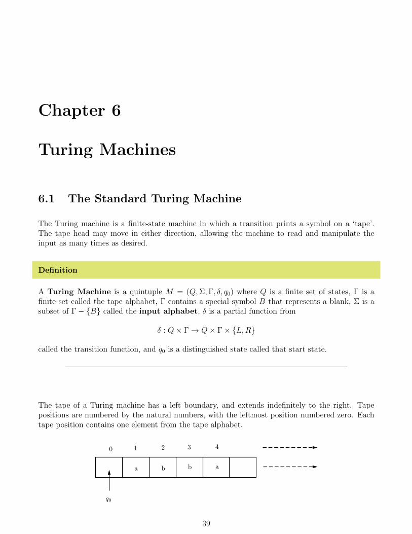
The tape of a Turing machine has a left boundary, and extends indefinitely to the right. Tapepositions are numbered by the natural numbers, with the leftmost position numbered zero. Eachtape position contains one element from the tape alphabet.
q0
a b b a
0 1 2 3 4
39
6.2. TURING MACHINES AS LANGUAGE ACCEPTORSCHAPTER 6. TURING MACHINES
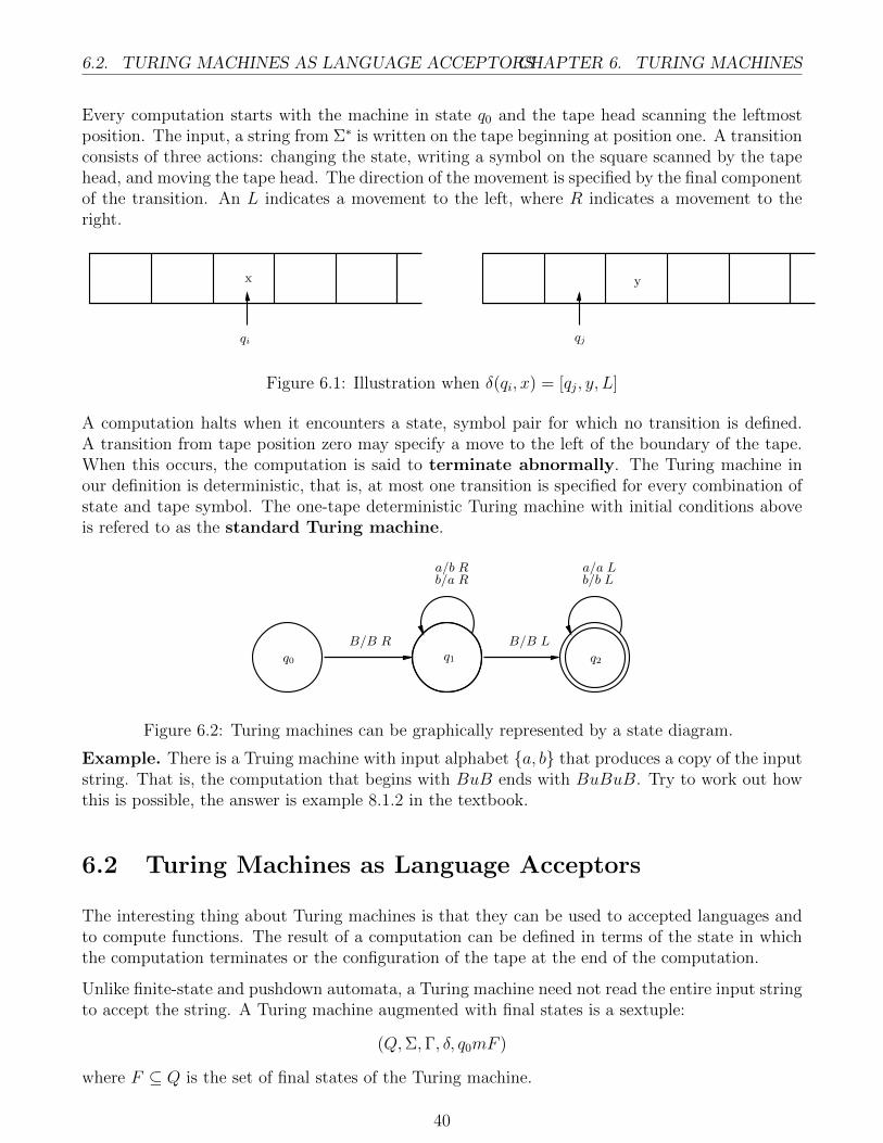
Every computation starts with the machine in state q0 and the tape head scanning the leftmostposition. The input, a string from Σ∗ is written on the tape beginning at position one. A transitionconsists of three actions: changing the state, writing a symbol on the square scanned by the tapehead, and moving the tape head. The direction of the movement is specified by the final componentof the transition. An L indicates a movement to the left, where R indicates a movement to theright.
qi qj
yx
Figure 6.1: Illustration when δ(qi, x) = [qj, y, L]
A computation halts when it encounters a state, symbol pair for which no transition is defined.A transition from tape position zero may specify a move to the left of the boundary of the tape.When this occurs, the computation is said to terminate abnormally. The Turing machine inour definition is deterministic, that is, at most one transition is specified for every combination ofstate and tape symbol. The one-tape deterministic Turing machine with initial conditions aboveis refered to as the standard Turing machine.
B/B R B/B L
a/b Rb/a R
a/a Lb/b L
q0 q1 q2
Figure 6.2: Turing machines can be graphically represented by a state diagram.
Example. There is a Truing machine with input alphabet {a, b} that produces a copy of the inputstring. That is, the computation that begins with BuB ends with BuBuB. Try to work out howthis is possible, the answer is example 8.1.2 in the textbook.
6.2 Turing Machines as Language Acceptors
The interesting thing about Turing machines is that they can be used to accepted languages andto compute functions. The result of a computation can be defined in terms of the state in whichthe computation terminates or the configuration of the tape at the end of the computation.
Unlike finite-state and pushdown automata, a Turing machine need not read the entire input stringto accept the string. A Turing machine augmented with final states is a sextuple:
(Q,Σ,Γ, δ, q0mF )
where F ⊆ Q is the set of final states of the Turing machine.
40
CHAPTER 6. TURING MACHINES 6.3. ALTERNATIVE ACCEPTANCE CRITERIA
Definition
Let M = (Q,Σ,Γ, δ, q0mF ) be a Turing machine. A string u ∈ Σ∗ is accepted by final stateif the computation of M with input u halts in a final state. A computation that terminatesabnormally rejects the input regardless of the state in which the machine halts. The language ofM , usually denoted L(M) is the set of all strings accepted by M .
A language accepted by a Turing machine is called a recursively enumerable language. Theability of a Turing machine to move in both directions and process blanks introduces the possibilitythat the machine may not halt for a particular input. Thus there are three possible outcomes fora Turing machine computation: it may halt and accept the input string; half and reject the string;or it may not halt at all. Because of the last possibility, we will sometimes say that a machine Mrecognizes L if it accepts L, but does not necessarily halt for all input strings. The computationsof M identify the strings L but may not provide answers for strings not in L. A language acceptedby a Turing machine that halts for all input strings is said to be recursive.
6.3 Alternative Acceptance Criteria
Using our prior definition, the acceptance of a string by a Turing machine is determined by thestate of the machine when the computation halts. Alternative approaches to defining acceptancewill be presented in this section.
Definition
Let M = (Q,Σ,Γ, δ, q0mF ) be a Turing machine. A string u ∈ Σ∗ is accepted by halting if thecomputation of M with input u halts normally.
Turing machines designed for acceptance by halting are used for language recognition. The com-putation for any input not in the language will not terminate. The next theorem shows thatany language recognized by a machine that accepts by halting is also accepted by a machine thataccepts by final state:Theorem 14. The following statements are equivalent:
1. The language L is accepted by a Turing machine that accepts by final state.
2. The language L is accepted by a Turing machine that accepts by halting.
41
6.4. MULTITRACK MACHINES CHAPTER 6. TURING MACHINES
6.4 Multitrack Machines
A multitrack tape is one in which the tape is divided into tracks. A tape position in an n-tracktape contains n symbols from the tape alphabet. The machine reads and entire tape position.Multiple tracks increase the amount of information that can be considered when determining theappropriate transition. A tape position in a two-track machine is represented by the ordered pair[x, y] where x is the symbol in track 1, and y is the symbol in track 2.
The states, input alphabet, tape alphabet, initial state, and final states of a two track machine arethe same as in the standard Turing machine. A two-track transition reads and rewrites the entiretape position. A transition of a two track machine is written as follows:
δ(qi, [x, y]) = [qj, [z, w], d]
where d ∈ {L,R}.Theorem 15. A language L is accepted by a two-track Turing machine if and only if it is acceptedby a standard Turing machine.
6.5 Two-Way Tape Machines
A Turing machine with a two-way tape is identical to the standard model except that the tapeextends indefinitely in both directions. Since a two-way tape has no left boundary, the input canbe placed anywhere on the tape. A”ll other tape positions are assumed to be blank. ”The tapehead is initially positioned on the blank to the immediate left of the input string. The advantageof a two way tape is that the Turing machine designed need not worry about crossing the leftboundary of the tape.
It turns out that this new type of Turing machine is completely the same as a regular Turingmachine:Theorem 16. A language L is accepted by a Turing machine with a two-way tape if and only ifit is accepted by a standard Turing machine.
6.6 Multitape Machines
A k-tape machine has k tapes and k independent tape heads. The states and alphabets of amultitape machine are the same as in a standard Turing machine. The machine reads the tapessimultaneously but has only on state- this is depicted by attaching each of the independent tapeheads to a single control indicating the current state.
A transition in a multitape machine may:
1. Change the state
2. Write a symbol on each of the tapes
3. Independently reposition each of the tape heads
42
CHAPTER 6. TURING MACHINES 6.7. NONDETERMINISTIC TURING MACHINES
The repositioning consists of moving the tape head one square to the right, one square to the left,or leaving it at its current position. A transition of a two-tape machine scanning x1 on tape 1 andx2 on tape 2 is written:
δ(qi, x1, x2) = [qj; y1, d1; y2, d2]
where xi, yi ∈ Γ and di ∈ [L,R, S]. This transition causes the machine to write yi on tape i. Thesymbol di represents the direction of the movement of tape head i.
The input to a multitape machine is placed in the standard position on tape 1. All the other tapesare assumed to be blank. The tape heads originally scan the leftmost position of each tape. Amultitape machine can be represented by a state diagram in which the label on an arc specifiesthe action of each tape.
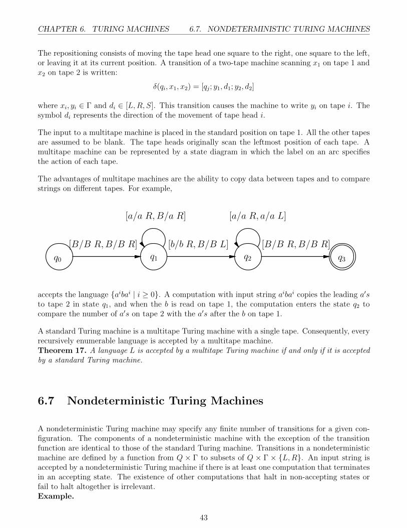
The advantages of multitape machines are the ability to copy data between tapes and to comparestrings on different tapes. For example,
[B/B R,B/B R]
[a/a R,B/a R]
[b/b R,B/B L]
[a/a R, a/a L]
[B/B R,B/B R]
q0 q1 q2 q3
accepts the language {aibai | i ≥ 0}. A computation with input string aibai copies the leading a′sto tape 2 in state q1, and when the b is read on tape 1, the computation enters the state q2 tocompare the number of a′s on tape 2 with the a′s after the b on tape 1.
A standard Turing machine is a multitape Turing machine with a single tape. Consequently, everyrecursively enumerable language is accepted by a multitape machine.Theorem 17. A language L is accepted by a multitape Turing machine if and only if it is acceptedby a standard Turing machine.
6.7 Nondeterministic Turing Machines
A nondeterministic Turing machine may specify any finite number of transitions for a given con-figuration. The components of a nondeterministic machine with the exception of the transitionfunction are identical to those of the standard Turing machine. Transitions in a nondeterministicmachine are defined by a function from Q × Γ to subsets of Q × Γ × {L,R}. An input string isaccepted by a nondeterministic Turing machine if there is at least one computation that terminatesin an accepting state. The existence of other computations that halt in non-accepting states orfail to halt altogether is irrelevant.Example.
43
6.8. TURING MACHINES AS LANGUAGE ENUMERATORSCHAPTER 6. TURING MACHINES
B/B R c/c R a/a R b/b R
c/c L
b/b L a/a L
a/a R
b/b R
c/c R
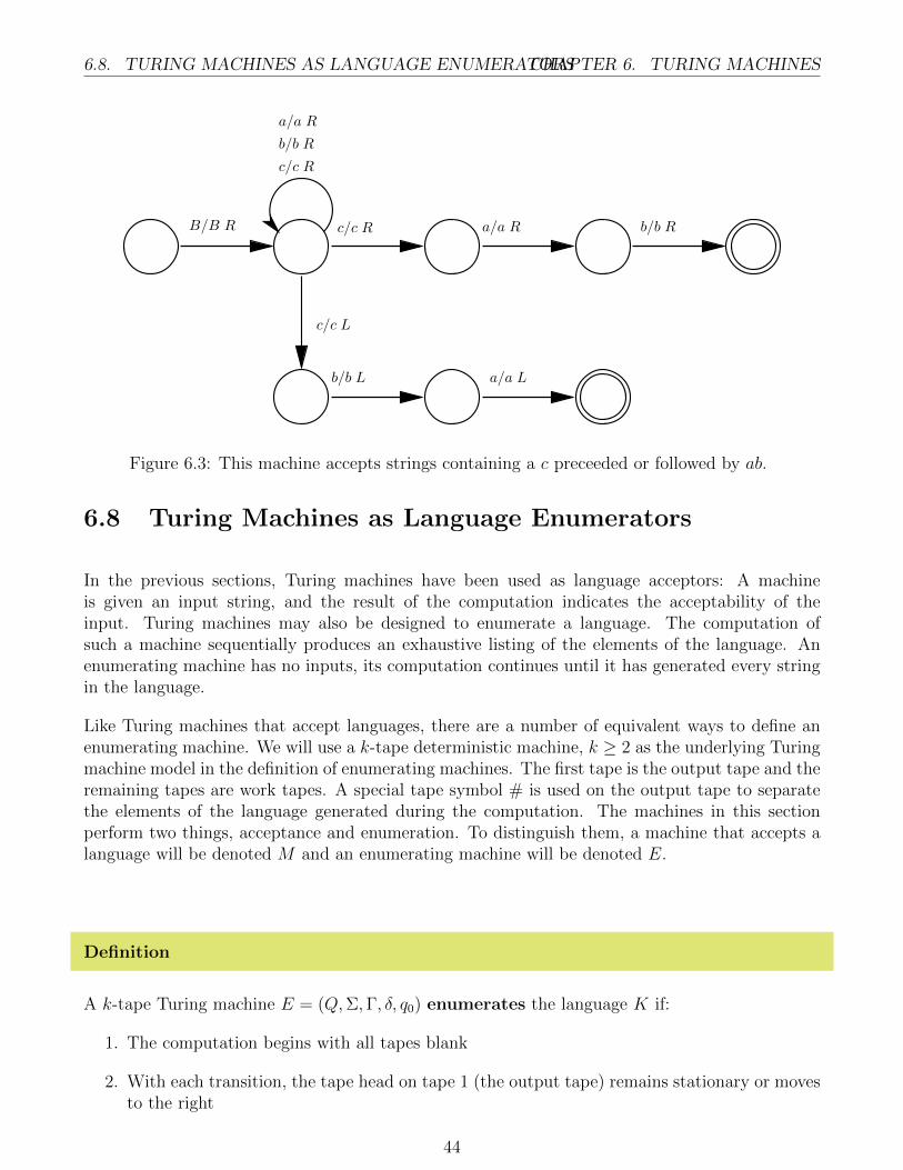
Figure 6.3: This machine accepts strings containing a c preceeded or followed by ab.
6.8 Turing Machines as Language Enumerators
In the previous sections, Turing machines have been used as language acceptors: A machineis given an input string, and the result of the computation indicates the acceptability of theinput. Turing machines may also be designed to enumerate a language. The computation ofsuch a machine sequentially produces an exhaustive listing of the elements of the language. Anenumerating machine has no inputs, its computation continues until it has generated every stringin the language.
Like Turing machines that accept languages, there are a number of equivalent ways to define anenumerating machine. We will use a k-tape deterministic machine, k ≥ 2 as the underlying Turingmachine model in the definition of enumerating machines. The first tape is the output tape and theremaining tapes are work tapes. A special tape symbol # is used on the output tape to separatethe elements of the language generated during the computation. The machines in this sectionperform two things, acceptance and enumeration. To distinguish them, a machine that accepts alanguage will be denoted M and an enumerating machine will be denoted E.
Definition
A k-tape Turing machine E = (Q,Σ,Γ, δ, q0) enumerates the language K if:
1. The computation begins with all tapes blank
2. With each transition, the tape head on tape 1 (the output tape) remains stationary or movesto the right
44
CHAPTER 6. TURING MACHINES6.8. TURING MACHINES AS LANGUAGE ENUMERATORS
3. At any point in the computation, the nonblank portion of tape 1 has the form
B#u1#u2#...#uk# or B#u1#u2#...#uk#v
where ui ∈ L and v ∈ Σ∗.
4. A string u will be written on tape 1 preceded and followed by # if and only if u ∈ L.
Theorem 18. Let L be a language enumerated by a Turing machine E. Then there is a Turingmachine E ′ that enumerates L and each string in L appears only once on the output tape of E ′.
Proof. The idea is essentially to add one more tape that acts as a ‘is this word already on theoutput tape’? Checker.
Theorem 19. If L is enumerated by a Turing machine, then L is recursively enumerable.
45
6.8. TURING MACHINES AS LANGUAGE ENUMERATORSCHAPTER 6. TURING MACHINES
46
Chapter 7
Turing Computable Functions
7.1 Computation of Functions
A function f : X → Y is a mapping that assigns at most one value from the set Y to each elementof the domain X. Adopting a computational viewpoint, we refer to the variables of f as theinput of the function. The definition of a function does not specify f(x). Turing machines will bedesigned to compute the values of functions. The domain and range of a function computed by aTuring machine consist of string over the input alphabet of the machines.
A Turing machine that computes a function has two distinguished states: the initial state q0 andthe halting state qf . A computation begins with a transition from state q0 that positions the tapehead at the beginning of the input string. The state q0 is never reentered; its sole purpose is toinitiate the computation. All computations that terminate do so in state qf with the value of thefunction written on the tape beginning at position one.
Definition
A deterministic one-tape Turing machine M = (Q,Σ,Γ, δ, q0, qf ) computes the unary functionf : Σ∗ → Σ∗ if
1. There is only one transition from the state q0 and it has the form δ(q0, B) = [qi, B,R].
2. There are no transitions of the form δ(qi, x) = [qo, y, d] for any qi ∈ Q, x, y inΓ and d ∈ {L,R}
3. THere are no transitions of the form δ(qf , B)
4. The computation with input u halts in the configuration qfBvB whenever f(u) = v;
5. The computation continues indefinitely whenever f(u) ↑
a Function is said to be Turing Computable if there is a Turing machine that computes it. A
47
7.2. NUMERIC COMPUTATION CHAPTER 7. TURING COMPUTABLE FUNCTIONS
Turing machine that computes a function f may fail to halt for an input string u. In this case, fis undefined for u. Thus Turing machines can compute both total and partial functions.
An arbitrary need not have the same domain and range. Turing machines can be designed tocompute functions from Σ∗ to a specific set R by designating an input alphabet Σ and range R.Condition 4 is then interpreted as requiring the string v to be an element of R.
B/B R
b/b RB/B R
a/a R
a/a Rb/b R
B/B L
a/B Lb/B L
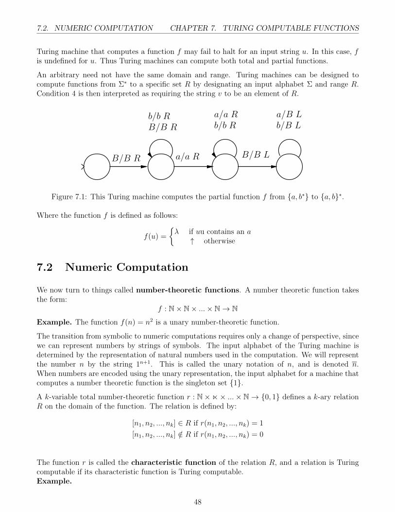
Figure 7.1: This Turing machine computes the partial function f from {a, b∗} to {a, b}∗.
Where the function f is defined as follows:
f(u) =
{λ if uu contains an a
↑ otherwise
7.2 Numeric Computation
We now turn to things called number-theoretic functions. A number theoretic function takesthe form:
f : N× N× ...× N→ N
Example. The function f(n) = n2 is a unary number-theoretic function.
The transition from symbolic to numeric computations requires only a change of perspective, sincewe can represent numbers by strings of symbols. The input alphabet of the Turing machine isdetermined by the representation of natural numbers used in the computation. We will representthe number n by the string 1n+1. This is called the unary notation of n, and is denoted n.When numbers are encoded using the unary representation, the input alphabet for a machine thatcomputes a number theoretic function is the singleton set {1}.
A k-variable total number-theoretic function r : N×n× ...× N→ {0, 1} defines a k-ary relationR on the domain of the function. The relation is defined by:
[n1, n2, ..., nk] ∈ R if r(n1, n2, ..., nk) = 1
[n1, n2, ..., nk] /∈ R if r(n1, n2, ..., nk) = 0
The function r is called the characteristic function of the relation R, and a relation is Turingcomputable if its characteristic function is Turing computable.Example.
48
CHAPTER 7. TURING COMPUTABLE FUNCTIONS7.3. SEQUENTIAL OPERATION OF TURING MACHINES
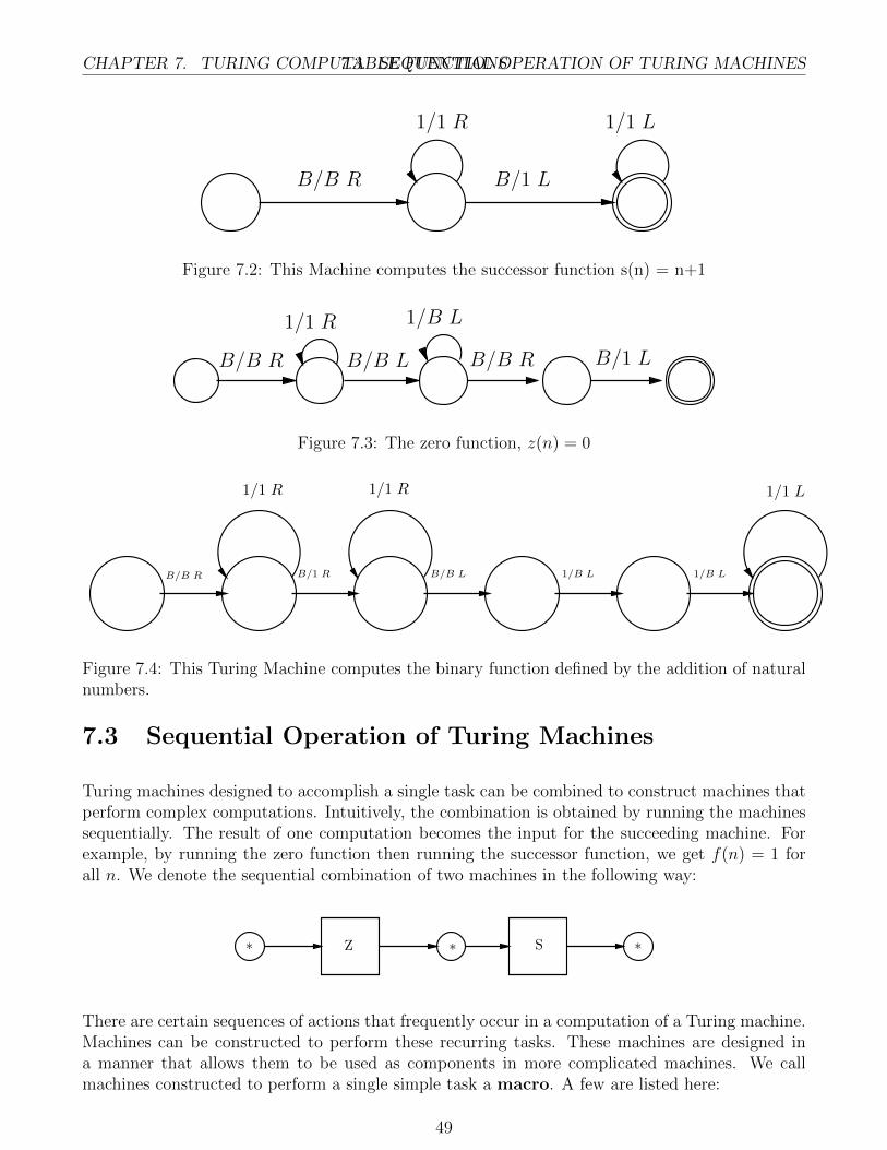
B/B R B/1 L
1/1 R 1/1 L
Figure 7.2: This Machine computes the successor function s(n) = n+1
B/B R
1/1 R
B/B L
1/B L
B/B R B/1 L
Figure 7.3: The zero function, z(n) = 0
B/B R B/1 R
1/1 R 1/1 R
B/B L 1/B L 1/B L
1/1 L
Figure 7.4: This Turing Machine computes the binary function defined by the addition of naturalnumbers.
7.3 Sequential Operation of Turing Machines
Turing machines designed to accomplish a single task can be combined to construct machines thatperform complex computations. Intuitively, the combination is obtained by running the machinessequentially. The result of one computation becomes the input for the succeeding machine. Forexample, by running the zero function then running the successor function, we get f(n) = 1 forall n. We denote the sequential combination of two machines in the following way:
Z S* **
There are certain sequences of actions that frequently occur in a computation of a Turing machine.Machines can be constructed to perform these recurring tasks. These machines are designed ina manner that allows them to be used as components in more complicated machines. We callmachines constructed to perform a single simple task a macro. A few are listed here:
49
7.4. COMPOSITION OF FUNCTIONSCHAPTER 7. TURING COMPUTABLE FUNCTIONS
1. MRi (move right) requires a sequence of at least i natural numbers to the immediate rightof the tape at the initiation of a computation.
2. MLk (move left)requires a sequence of at least i natural numbers to the immediate left ofthe tape at the initiation of a computation.
3. FR and FL are the ‘fine’ macros, which move the tape head into a position to process thefirst natural number to the right or left of the current position.
4. Ek (erase) erases a sequence of k natural numbers and halts with the tape head in its originalposition.
5. CPYk and CPYk,i produce a copy of the designated number of integers. The segment of thetape on which the copy is produced is assumed to be blank- CPYk,i expects a sequence ofk + 1 numbers followed by a blank segment large enough to hold a copy of the first k.
6. T (translate) is the translate macro, and changes the location of the first natural number tothe right of the of the tape head.
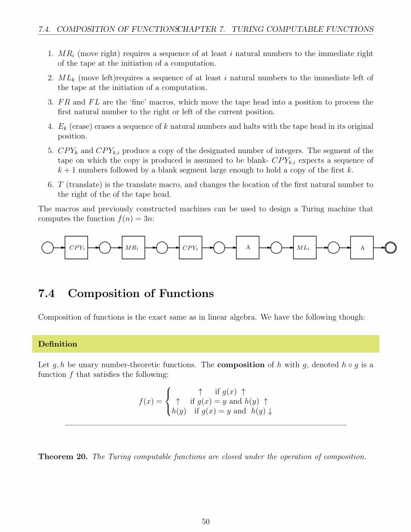
The macros and previously constructed machines can be used to design a Turing machine thatcomputes the function f(n) = 3n:
CPY1 MR1 CPY1 A ML1 A
7.4 Composition of Functions
Composition of functions is the exact same as in linear algebra. We have the following though:
Definition
Let g, h be unary number-theoretic functions. The composition of h with g, denoted h ◦ g is afunction f that satisfies the following:
f(x) =
↑ if g(x) ↑
↑ if g(x) = y and h(y) ↑h(y) if g(x) = y and h(y) ↓
Theorem 20. The Turing computable functions are closed under the operation of composition.
50
Chapter 8
The Chomsky Hierarchy
8.1 Unrestricted Grammars
The components of a phase-structure grammar are the same as those of the regular and context-freegrammars studied in chapter 3. A phase-structure grammar consists of a finite set V of variables,an alphabet Σ, a start variable, and a set of rules. A rule has the form u → v where u, v canbe any combination of variables and terminals, and defines a permissible string of transformation.The application of a rule to a string z is a two step process consisting of:
1. Matching the left-hand side of the rule to a substring of z, and
2. Replacing the left-hand side with the right-hand side.
The unrestricted grammars are the largest class of phase-structure grammars. There are no con-straints on a rule other than requiring that the left-hand must not be null.
Definition
An unrestricted grammar is a quadruple (V,Σ, P, S) where V is a finite set of variables; Σ isa finite set of terminal symbols, P is a set of rules, and S is a distinguished element of V . Aproduction of an unrestricted grammar has the form u→ v where u ∈ (V ∪Σ)+ and v ∈ (V ∪Σ)∗.The sets V and Σ are assumed to be disjoint.
Example. The unrestricted grammar with V = {S,A,C},Σ = {a, b, c} and rules:
S → aAbc | λA→ aAbC | λCb→ bC
Cc→ cc
51
8.2. CONTEXT- SENSITIVE GRAMMARS CHAPTER 8. THE CHOMSKY HIERARCHY
with a start symbol S generates the language {aibici | i ≥ 0}. The rule Cb→ bC allows the finalC to pass through the b′s that separate it from the c′s at the end of the string.Theorem 21. Let G = (V,Σ, P, S) be an unrestricted grammar. Then L(G) is a recursivelyenumerable language.
8.2 Context- Sensitive Grammars
The context-sensitive grammars represent an intermediate step between context-free and unre-stricted grammar. No restrictions are placed on the left handed side of a production, but thelength of the right hand side is required to be at least that of the left.
Definition
A phase-structure grammar G = (V,Σ, P, S) is called context-sensitive if each rule has the formu→ v where u ∈ (V ∪ Σ)+, and length(u) ≤ length(v).
Example. The following rules generate the language {aibici | i > 0}, and satisfy the conditions ofa context-sensitive rules.
S → aAbc | abcA→ aAbC | abC
Theorem 22. Every context-sensitive grammar is recursive.
8.2.1 Linear-Bounded Automata
Restricting the amount of tape that a Turing machine can use decreases the capabilities of a Turingmachine. A linear-bounded automaton is a Turing machine in which the amount of available tapeis determined by the length of the input string. The input alphabet contains two symbols, < and>, that designate the left and right boundaries of the tape.
Definition
A linear-bounded automaton (LBA) is a structureM = (Q,Σ,Γ, δ, q0, <,>, F ). WhereQ,Σ,Γ, δ, q0,and F are the same as for a nondeterministic Turing machine. The symbols < and > are distin-guished elements of Σ.
52
CHAPTER 8. THE CHOMSKY HIERARCHY 8.2. CONTEXT- SENSITIVE GRAMMARS
Theorem 23. Let L be a context-sensitive language. Then there is a linear bounded automatonM with L(M) = L.Theorem 24. Let L be a language accepted by a linear bounded automaton. Then L − {λ} is acontext-sensitive language.
8.2.2 Chomsky Hierarchy
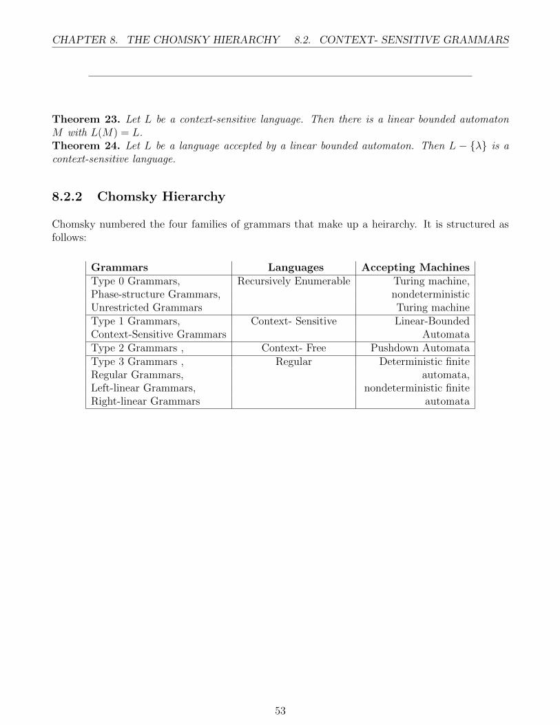
Chomsky numbered the four families of grammars that make up a heirarchy. It is structured asfollows:
Grammars Languages Accepting MachinesType 0 Grammars, Recursively Enumerable Turing machine,Phase-structure Grammars, nondeterministicUnrestricted Grammars Turing machineType 1 Grammars, Context- Sensitive Linear-BoundedContext-Sensitive Grammars AutomataType 2 Grammars , Context- Free Pushdown AutomataType 3 Grammars , Regular Deterministic finiteRegular Grammars, automata,Left-linear Grammars, nondeterministic finiteRight-linear Grammars automata
53
8.2. CONTEXT- SENSITIVE GRAMMARS CHAPTER 8. THE CHOMSKY HIERARCHY
54
Chapter 9
Decidability and Undecidability
A decision problem P is a set of related questions, each of which has a yes or no answer.The decision problem of determining if a number is a perfect square consists of the followingquestions:
p0 : Is 0 a perfect square?
p1 : Is 1 a perfect square?
p2 : Is 2 a perfect square?
A decision is said to be decidable if it has a solution. A solution to a decision problem is analgorithm that determines the appropriate answer to every questions p ∈ P.
9.1 Church-Turing Thesis
Theorem 25. There is an effective procedure to solve a decision problem if and only if there is aTuring machine that halts for all input strings and solves the problem.Theorem 26. A decision problem P is partially solvable if and only if there is a Turing machinethat accepts precisely the instances of P whose answer is yes.Theorem 27. A function f is effectively computable if and only if there is a Turing machine thatcomputes f .
9.2 Universal Machines
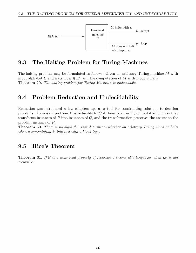
A universal Turing machine is designed to simulate the computations of an arbitrary Turingmachine M . To do so, the input to the universal machine must contain a representation of themachine M and the string w to be processed by M . For simplicity, we will assume that M is astandard Turing machine that accepts by halting. The action of a universal machine U is depictedby:Theorem 28. The language LH = {R(M)w | M halts with input w }.
55
9.3. THE HALTING PROBLEM FOR TURING MACHINESCHAPTER 9. DECIDABILITY AND UNDECIDABILITY
R(M)w
Universal
machine
U
M halts with w
M does not halt
with input w
accept
loop
9.3 The Halting Problem for Turing Machines
The halting problem may be formulated as follows: Given an arbitrary Turing machine M withinput alphabet Σ and a string w ∈ Σ∗, will the computation of M with input w halt?Theorem 29. The halting problem for Turing Machines is undecidable.
9.4 Problem Reduction and Undecidability
Reduction was introduced a few chapters ago as a tool for constructing solutions to decisionproblems. A decision problem P is reducible to Q if there is a Turing computable function thattransforms instances of P into instances of Q, and the transformation preserves the answer to theproblem instance of P .Theorem 30. There is no algorithm that determines whether an arbitrary Turing machine haltswhen a computation is initiated with a blank tape.
9.5 Rice’s Theorem
Theorem 31. If P is a nontrivial property of recursively enumerable languages, then LP is notrecursive.
56

Chapter 10
µ-Recursive Functions
A family of intuitively computable number-theoretic functions, known as the primitive recursivefunctions, is obtained from the basic functions:
1. The successor function s : s(x) = x+ 1
2. The zero function z : z(x) = 0
3. The projection function p(n)i : p
(n)i (x1, x2, ...xn) = xi, 1 ≤ i ≤ n
Definition
Let g and h be total number-theoretic functions with n and n+2 variables, respectively. The n+1variable function f defined by:
f(x1, ...xn, 0) = g(x1, ..., xn)
f(x1, ...xn, y + 1) = h(x1, x2, ...xn, y, f(x1, ...xn, y))
Is said to be obtained from g and h by primitive recursion
Where xi is said to be the parameters for a definition by primitive recursion, and y is said to bethe recursive variable. The algorithm for computing f(x1, ..., xn, y) whenever g, h are availablefollows from our definition. We have the following:
f(x1, ...xn, 0) = g(x1, ...xn)
And since f(x1, ...xn, y) is obtained from h by using the parameters x1, ...xn, treating y as arecursive variable, and f(x1, ...xn, y) as the previous value of the function, we have a definition forf .
57
CHAPTER 10. µ-RECURSIVE FUNCTIONS
Definition
A function is primitive recursive if it can be obtained from the successor, zero, and projectionfunctions by a finite number of applications of composition and primitive recursion.
Example. f = add can be calculated from g(x) = x and h(x, y, z) = z + 1 by the following:
add(x, 0) = g(x) = x
add(x, y + 1) = h(x, y, add(x, y)) = add(x, y) + 1
Theorem 32. Every primitive recursive function is Turing computableTheorem 33. Let g be a primitive recursive function and f a total function that is identical to gfor all but a finite number of input values. Then f is primitive recursive.
58
Chapter 11
Time Complexity
Definition
Let f : N→ N and g : N→ N be one-variable number-theoretic functions.
1. The function f is said to be of order g if there exists a positive constant c and a naturalnumber n0 such that f(n) ≤ cg(n) for all n ≥ n0.
2. The set of all functions of order g is denoted O(g) = {f |f is of order g }
When f is of order g we say that g provides an asymptotic upper bound on f .Example. Let f = n2, g = n3. Then, f ∈ O(g) but g /∈ O(f).
If f has the same rate of growth as g, then g is said to be an asympotically tight bound on f . Theset:
Θ(g) = {f | f ∈ O(g) and g ∈ O(f)}
Theorem 34. Let f be a polynomial of degree r. Then:
1. f ∈ Θ(nr)
2. f ∈ O(nk) for all k > r
3. f /∈ O(nk) for all k < r
Definition
59
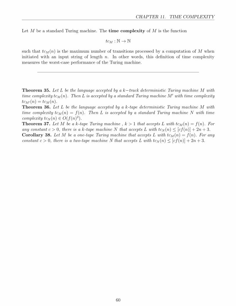
CHAPTER 11. TIME COMPLEXITY
Let M be a standard Turing machine. The time complexity of M is the function
tcM : N→ N
such that tcM(n) is the maximum number of transitions processed by a computation of M wheninitiated with an input string of length n. In other words, this definition of time complexitymeasures the worst-case performance of the Turing machine.
Theorem 35. Let L be the language accepted by a k−track deterministic Turing machine M withtime complexity tcM(n). Then L is accepted by a standard Turing machine M ′ with time complexitytcM ′(n) = tcM(n).Theorem 36. Let L be the language accepted by a k-tape deterministic Turing machine M withtime complexity tcM(n) = f(n). Then L is accepted by a standard Turing machine N with timecomplexity tcN(n) ∈ O(f(n)2).Theorem 37. Let M be a k-tape Turing machine , k > 1 that accepts L with tcM(n) = f(n). Forany constant c > 0, there is a k-tape machine N that accepts L with tcN(n) ≤ [cf(n)] + 2n+ 3.Corollary 38. Let M be a one-tape Turing machine that accepts L with tcM(n) = f(n). For anyconstant c > 0, there is a two-tape machine N that accepts L with tcN(n) ≤ [cf(n)] + 2n+ 3.
60
Chapter 12
P ,NP, and Cook’s Theorem
61